TwinTex: Geometry-aware Texture Generation for Abstracted 3D Architectural Models
Abstract.
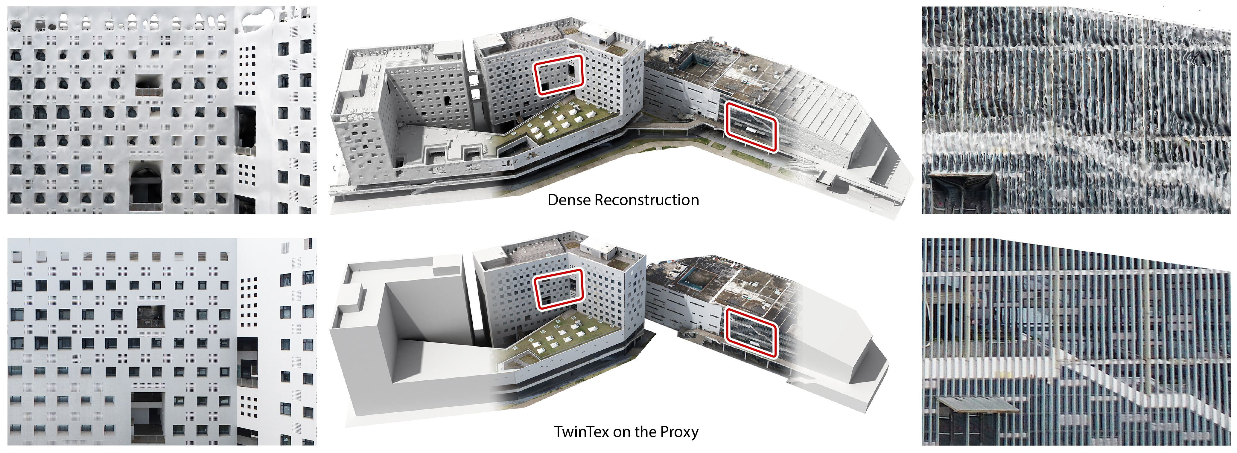
Coarse architectural models are often generated at scales ranging from individual buildings to scenes for downstream applications such as Digital Twin City, Metaverse, LODs, etc. Such piece-wise planar models can be abstracted as twins from 3D dense reconstructions. However, these models typically lack realistic texture relative to the real building or scene, making them unsuitable for vivid display or direct reference. In this paper, we present TwinTex, the first automatic texture mapping framework to generate a photo-realistic texture for a piece-wise planar proxy. Our method addresses most challenges occurring in such twin texture generation. Specifically, for each primitive plane, we first select a small set of photos with greedy heuristics considering photometric quality, perspective quality and facade texture completeness. Then, different levels of line features (LoLs) are extracted from the set of selected photos to generate guidance for later steps. With LoLs, we employ optimization algorithms to align texture with geometry from local to global. Finally, we fine-tune a diffusion model with a multi-mask initialization component and a new dataset to inpaint the missing region. Experimental results on many buildings, indoor scenes and man-made objects of varying complexity demonstrate the generalization ability of our algorithm. Our approach surpasses state-of-the-art texture mapping methods in terms of high-fidelity quality and reaches a human-expert production level with much less effort.
1. Introduction
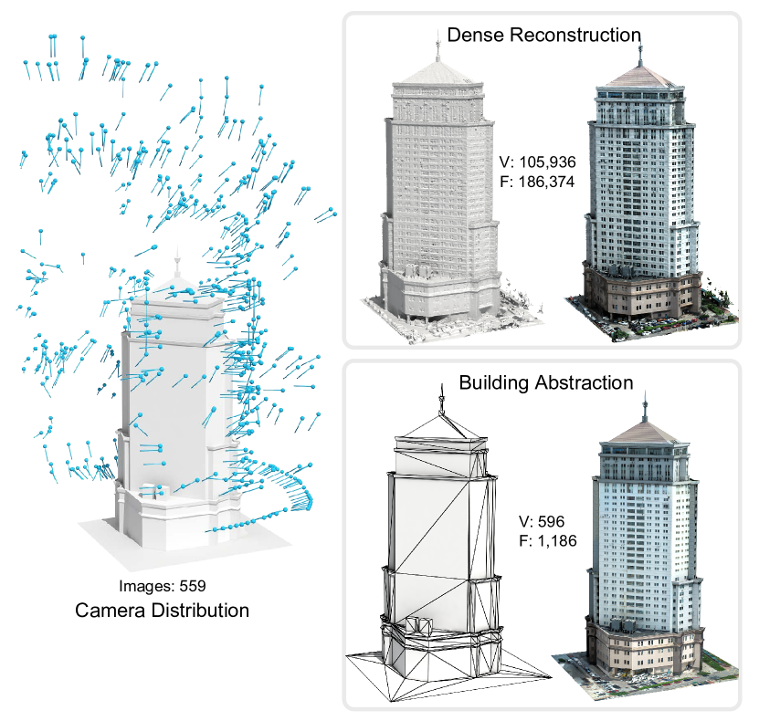
With the advances in active sensors (e.g., LiDAR), fully automated Multiple View Stereo (MVS) and aerial-based photogrammetry sensing technology, many mature algorithms have been developed to generate complete and high-fidelity 3D dense reconstruction (Musialski et al., 2013; Smith et al., 2018; Zhou et al., 2020) with textures (Waechter et al., 2014). Architectural models with simplified topology and twin shapes of such dense models can be generated from procedural modeling, approximated from dense reconstruction, or created manually by artists and architects. These abstracted twin models are tractable in plenty of downstream applications due to their sharper features, much lower needs on storage, and more suitable for transmission and real-time rendering, as shown in Fig. 2.
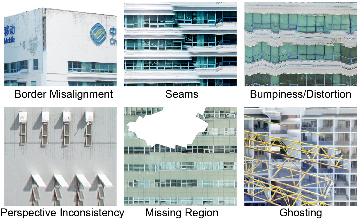
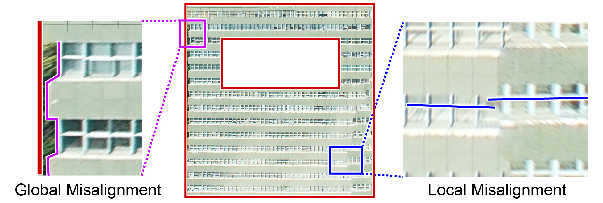
However, the texture information contained in the original dense reconstruction is often not maintained after abstraction. Thus, with all the calibrated RGB images, how to texture the twin proxy for the level of realism then becomes a challenging problem. An intuitive way is to employ image-based texture generation methods (Lempitsky and Ivanov, 2007; Waechter et al., 2014; Zhou and Koltun, 2014). However, these approaches would produce distorted and misaligned artifacts as illustrated in Fig. 3. Although patch-based optimization method (Bi et al., 2017) can reduce such artifacts to some extent by synthesizing photometrically-consistent aligned images to correct misalignments, it would possibly deliver blurring textures or missing regions. These issues are mainly caused by: i) the inaccurate camera parameters, ii) the significant geometric differences between the twin mesh and ground-truth models brought by the abstraction process, and iii) the large difference among viewing angles. The combination of these cases makes our problem even more challenging and complicated. The urban proxy models often exhibit large-scale planar structures. In practice, the modeling artists often manually create high-quality textures plane-by-plane. This is an extremely tedious, time-consuming, and labor-intensive process. It took quite a few days for a professional modeler to texture an abstracted model such as the Polytech shown in Fig. 1 with real photos. Texturing a model with a higher level of detail would take much longer.
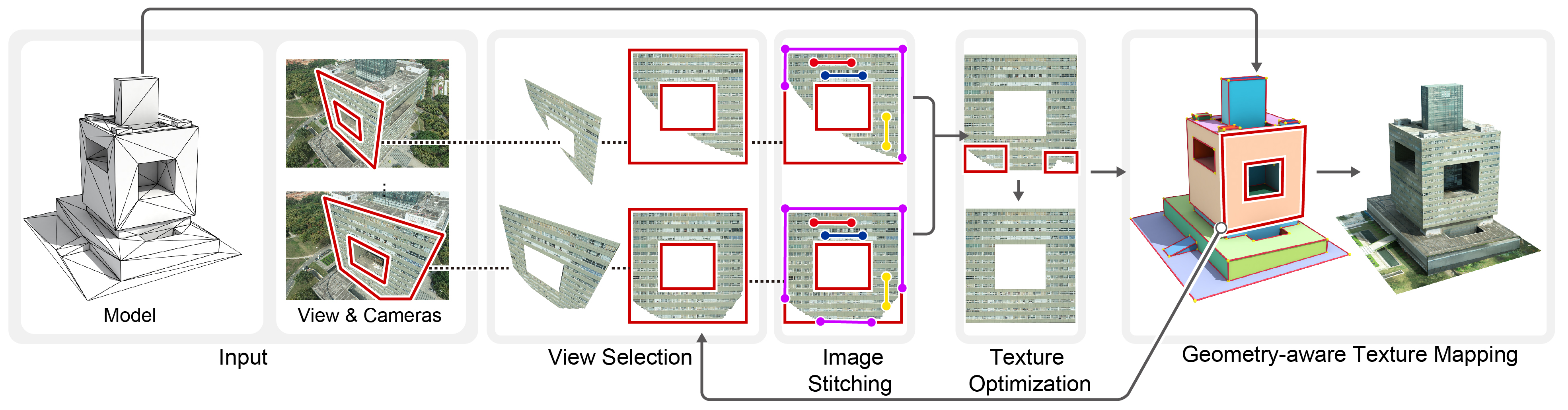
In this paper, we propose a plane-based methodology and fully automated algorithms to generate high-quality texture maps for piece-wise planar architectural models given a large set of unordered RGB photos. Our method addresses most challenges occurring in such twin texture generation: the large number and high resolution of input images, their drastically varying properties such as photometric quality, perspective quality (large variation of viewing angles), heavy occludes (e.g., trees and buildings), and texture-geometry misalignment (introduced by incorrect camera parameters and model abstraction process). Given a coarse model, our algorithm decomposes it into a set of planar polygonal shapes, for each of which we aim at generating a high-quality and complete texture map. We first present a plane-oriented view selection approach to select views that best cover each planar shape with high photometric and perspective consistency. Based on the line segments extracted from each view, a line-guided texture stitching is introduced to create a single texture map to preserve geometric features. Finally, we perform texture optimization to improve the illumination consistency and fill the missing regions in the texture map. Experiments are performed to show the effectiveness and robustness of our method. In summary, our work makes the following contributions:
-
•
A fully automatic TwinTex, which produces high-quality and geometry-aware texture for a simplified proxy model.
-
•
A view selection algorithm that can select a small number of candidate photos for each primitive plane considering texture completeness, perspective and photometric quality.
-
•
A plane-based texture mapping methodology via geometry-aware image stitching guided by LoLs.
-
•
An architectural dataset including various scenes and building components. We utilize this dataset and fine-tune a diffusion probabilistic model with a novel multi-mask initialization component to complete the texture maps.
2. Related Work
2.1. Image-based Texture Mapping
Texture mapping is an important approach for authoring photo-realistic 3D objects without increasing their geometric complexity (Yuksel et al., 2019). View-dependent texture mapping works (Debevec et al., 1996, 1998) composite multiple views of a scene by assuming the existence of a global mesh and storing all appearance variation in textures. Although they also use a view selection procedure to project a single image onto the model and then merge several image projections, they only determine for each polygon in the model in which photos it is visible. Instead, we present a novel view selection algorithm that considers texture completeness, perspective quality, and photometric quality.
To generate a single consistent texture map, early works on image-based texture mapping usually select multiple images for each face and blend them into textures by using different weighting strategies (Bernardini et al., 2001; Callieri et al., 2008). However, such methods could generate blurry and ghosting results due to camera calibration errors and inaccurate geometry. To reduce those artifacts caused by multi-image blending, later approaches choose to select only one view per face, then conduct seam optimization to create a texture patch and to avoid visible seams between adjacent patches (Lempitsky and Ivanov, 2007; Wang et al., 2018; Gal et al., 2010; Waechter et al., 2014; Fu et al., 2018, 2020). They typically solve a discrete labeling problem by using different data terms and smoothness terms to construct the Markov random field to select an optimal texture image for each face. Whereas, these approaches still suffer from misaligned seams in challenging cases. Another category of warping-based methods jointly rectifies the camera poses and geometric errors. Zhou and Koltun (2014) use local image warping to optimize camera poses in tandem with non-rigid correction functions for all images. This approach is then extended by (Bi et al., 2017) to propose a patch-based optimization that handles larger geometry inaccuracies by correctly aligning the input images. This method estimates the bidirectional similarity of different images, which suffers from high computational costs.
Although high-quality texture maps can be generated from the above methods, the resultant quality of texture mapping still greatly depends on the quality of reconstruction and accuracy of camera calibration. None of them can be naively applied to generate the realistic texture of a large-scale structured building or scene. Firstly, the abstracted proxy model has significant structural differences from the original dense mesh. Moreover, constrained by the complicated environment, the collected aerial data often has highly uneven camera distribution, large camera calibration errors and large variations in viewing angles. Current methods still cannot handle these problems well, resulting in obvious artifacts. Instead, we choose to generate texture in a plane-based manner that is more intuitive and human alike.
2.2. Structure-aware Scene Reconstruction and Texturing
Creating structured models from noisy raw data has become an ever-increasing demand in urban digitization. Ceylan et al. (2012, 2014) propose image-based 3D urban building reconstruction frameworks by exploiting the presence of linear and symmetric features (e.g., lines, repeated elements) in facade for image registration and 3D reconstruction. To generate simplified meshes, a popular way is to first reconstruct a 3D dense mesh and then simplify it using geometry simplification (Garland and Heckbert, 1997) or piece-wise planar structure approximation methods (Cohen-Steiner et al., 2004; Verdie et al., 2015; Salinas et al., 2015). Another way is to directly detect a set of planar primitives from the point clouds, then explore the arrangements of primitives to provide a compact polygonal mesh (Monszpart et al., 2015; Nan and Wonka, 2017; Fang and Lafarge, 2020; Bauchet and Lafarge, 2020; Bouzas et al., 2020; Pan et al., 2022; Guo et al., 2022). In practice, such proxy models are usually generated manually or by procedural modeling (Sinha et al., 2008) with arbitrary topology (e.g., manifolds or non-manifolds).
However, texturing such abstracted building models has drawn less attention. Several methods take into account the generation of texture maps while conducting a lightweight geometric reconstruction (Sinha et al., 2008; Garcia-Dorado et al., 2013; Huang et al., 2017; Maier et al., 2017; Wang and Guo, 2018). For example, Garcia-Dorado et al. (2013) computes a per-building volumetric proxy, then uses a surface graph-cut method to stitch aerial images and yield a visually coherent texture map. However, their reconstruction results are 2.5D which can only restore textures under limited perspectives, losing important structures. Recently, deep learning approaches based on image-image translation networks have been proposed to synthesize texture details for coarse meshes of urban areas (Kelly et al., 2018; Georgiou et al., 2021). Although data-driven methods are able to generate various styles of textures, they require extensive training sets, and the synthesized textures lack realism comparing to the original real scenes. The technique of NeRF (Müller et al., 2022) shows great ability to generate high-quality 3D shapes and textures (Metzer et al., 2022; Baatz et al., 2022). However, remember that we aim at very high-resolution input and output images which require extremely large memory, employing a small set of input images is not enough for NeRF-based methods to generate satisfying results, which makes them less applicable in our scenario.
2.3. Image Stitching and Completion
Image stitching is to combine multiple images with overlapping sections to produce a single panoramic or high-resolution image (Szeliski et al., 2007; Mehta and Bhirud, 2011). Early methods estimate an optimal global transformation for each input image (Brown and Lowe, 2007). However, they only work well for scenes near planar or with slight view disparity, and usually generate ghosting artifacts or projective distortion for general scenes. For more accurate stitching, many approaches adopt spatially-varying warps to process different regions of an image, including smoothly varying affine transformation (Lin et al., 2011), dual or quasi homographies (Gao et al., 2011; Li et al., 2017), shape-preserving half-projective warps (Chang et al., 2014; Lin et al., 2015), and smoothly varying homography field (Zaragoza et al., 2013), etc. Aiming at building facades, Musialski et al. (2010) present a system for generating approximately orthographic facade textures from a set of perspective photographs. They perform multi-view image stitching over planar proxies by using a gradient-domain stitching to avoid visible seams.
However, they are usually time-consuming and unsuitable for scenes with large parallax and view disparity. Several methods are then proposed to obtain better alignment with less distortion, especially for large parallax (Zhang et al., 2016; Lee and Sim, 2020), but linear structures in the image are not well maintained. After that, instead of just using point feature matching, line features are introduced to preserve both linear structures (Li et al., 2015; Xiang et al., 2018; Liao and Li, 2019; Jia et al., 2021). All these methods apply a uniform grid to warp the images, which are not flexible enough to align the regions with dense geometric features. Unlike them, we propose to use an adaptive grid to locally warp the images and better align the large-scale line features.
Image completion, also known as image inpainting, is the process of restoring missing or damaged areas in an image. Extensive research has been conducted on image completion, and existing methods can be classified into three types: 1) diffusion-based methods, 2) patch-based methods and 3) deep learning methods based on generative models. A detailed review is out of the scope of this paper, and we refer the reader to recent works (Dhariwal and Nichol, 2021; Lugmayr et al., 2022) and surveys (Guillemot and Meur, 2014; Rojas et al., 2020; Elharrouss et al., 2020; Jam et al., 2021).
3. Problem Statement and Overview
The objective of our approach is to automatically generate realistic and geometry-aware texture maps for a piece-wise planar model, i.e., urban building or scene. Our algorithm takes a set of calibrated camera views and an abstracted model as input, and outputs high-quality texture maps. The proxy model is a polygonal mesh consisting of a set of planar polygonal shapes , each of which is referred to as a proxy polygon.
To produce a texture map for each proxy polygon , the first step should be to select one or multiple images as candidate maps for . However, unlike previous texturing problems dealing with dense models (small triangles), it is usual that none of the given images can cover such large proxy polygons in abstracted versions. Hence, we employ the latter scheme and select multiple images for each polygon shape. However, there are still several challenges that exist in our scenario: i) Photometric issue. There are seams, illumination resolution inconsistency between adjacent patches. For large scale scenes, the frequent ghosting effect is mainly introduced by the dynamic instances, such as cars and tower crane. ii) Perspective issue. Even with photometric consistent patches, it would still be apparent that the stitched texture comes from several images with largely varied viewing angles. iii) Image-to-image and image-to-geometry misalignment. This is introduced by both the inaccuracy of camera parameters and the simplification process. iv) Facade incompleteness. In the absence of semantic guidance, how to fill a largely empty region with geometrically and semantically consistent content remains a problem.

To address the above problems, we propose a plane-based and geometry-aware texture mapping methodology, as shown in Fig. 4. First, we extract high-quality views and visible regions for each proxy polygon . An effective greedy heuristic method is proposed to select a small set of views that best cover each with high photometric and perspective consistency (Sec. 4). Next, in Sec. 5.1, the rich line features contained in the selected images are detected and organized into Level of Lines (LoLs). After that, all the selected images are sequentially warped to their relative proxy boundary based on LoLs and stitched into a single texture map. Sec. 5.2 provides details. Then, each texture map is optimized by a series of operators to reveal illumination consistency. Finally, we provide an architectural image dataset and train a multi-mask Diffusion Model to inpaint the missing regions in texture maps, see Sec. 5.3. Our algorithm has been implemented as a customized plug-in of a widely used graphics engine called Houdini111https://www.sidefx.com/.
4. Plane-oriented View Selection
Proxy polygon extraction.
The input proxy can be created manually, generated procedurally, or abstracted from a dense reconstruction. is a polygonal mesh where each basic element of is an edge and is either a polygonal or triangular facet, as shown in Fig. 5. We first segment into a set of planar polygonal shapes, each of which is represented as a proxy polygon . We input by utilizing a region-growing algorithm based on face normal. We then detect the corresponding proxy boundary by choosing and sorting the boundary edges of . Fig. 5 shows the result of this step on the scene of Hitech.
View selection. Given a large set of input calibrated photos, the goal of this step is to select a small set of camera views as candidate feature maps to best cover each proxy polygon . We first apply frustum-culling and visibility detection to filter out the views and pixels which are invisible, far away from , or have extremely inclined viewing angles. The filtered images are then projected onto , and the projected regions covering the proxy polygon are extracted as candidate images, as shown in Fig. 4.
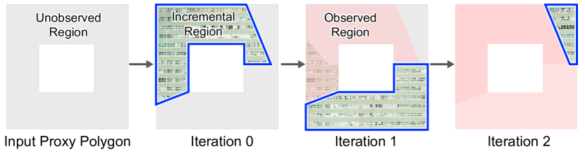
Next, we propose an iterative view selection algorithm to select a smaller set of candidate views from the projected images covering (see Fig. 6). Starting from an empty set , we select the best projected image with the highest quality (denoted by ) in each iteration to create . This process converges when there is no projected image left to examine, or the can fully cover , i.e., the area of unobserved regions in is smaller than a given threshold . We measure the quality of each by its incremental coverage ratio of the proxy polygon, its photometric and perspective quality and consistency with . The score is calculated as the weighted sum of two terms:
| (1) |
where and represent the photometric and perspective quality, respectively. is the weight of .
Photometric quality.
This term favors with large incremental projection region, high resolution, and high photometric similarity to all the projected images and previously selected images. In detail, the coverage ratio of against proxy polygon at iteration is calculated as /. It is determined by the area of the incremental region normalized with the unobserved area . Second, we measure the resolution of as by computing the average of the gradient magnitude over all pixels within the projection region (Gal et al., 2010). The photometric similarity, , is defined by checking the photo-consistency of against all the other projected images. It is computed by a multi-variate Gaussian function (Waechter et al., 2014). Furthermore, we introduce a new smoothness term to give a more confident value to a projected image when is consistent with the current set of selected images . The final photometric quality term is organized as:
| (2) | |||
| (3) |
where and are the respective weight of and , is the weight of . represents the mean of pixel-wise color difference between the overlapping pixels of image and all the images in after normalization. if iteration is zero or there exists no overlapping regions. The quality term tends to select a set of projected images with the maximum photometric and content consistency, which helps reducing the ghosting effect. Note that both photometric and smoothness terms consider overlap regions. directly uses the whole projected regions (including overlap regions) of all the projected images . Meanwhile, the smoothness term only considers the overlap region compared to the candidate projected image .
Pespective quality.
However, only considering the photometric quality will possibly cause significant perspective inconsistency among selected regions/patches. An example is shown at the bottom left in Fig. 3, where the partial region is from the left viewing angles and the other regions come from the right viewing angles. One solution is to evaluate one patch at a time and choose patches with viewing directions as close to the normal of the current proxy polygon as possible (Wang et al., 2018). However, the set of candidate photos usually has a large variation in viewing direction and extremely uneven distribution, especially for those proxy polygons with large planes. Strong front-parallel constraint could introduce missing regions while loose constraint could cause significant perspective differences. To address this issue, we present a novel quality measurement to select a set of perspective consistent images, while satisfying the front-parallel constraint as much as possible.
The perspective quality term tends to select the next candidate image with a viewing direction similar to selected images in , and with a viewing angle perpendicular to as much as possible. Hence, the perspective property is measured with front-parallel constraint and viewing angle consistency against selected photos. Unlike previous methods that only consider the viewing angle of a single candidate at a time (Wang et al., 2018), we propose to select a set of candidate images with high viewing angle consistency and as many front-parallel properties. Photo collections usually have a large variety of viewing angles. In practice, it is difficult to find a set of photos from the input all with a high level of front-parallelism covering a large plane. Compared to focusing on front-parallelism, we hope to stress more on viewing direction consistency as gets larger. Hence, we introduce the inverse facade normal as the first selected viewing direction. We define the perspective quality as:
| (4) |
where is the number of selected images in , is the plane normal of , is the viewing direction of , is the viewing direction of the -th image in . calculates the normalized angular distance between facet normal and plane normal . calculates the normalized angular distance between facet normal and .
5. Line-guided Texture Mapping
After determining a set of high-quality images for each proxy polygon , our next goal is to generate a realistic and geometry-aware texture map for . Urban buildings usually exhibit rich structural information, such as local/global line features (e.g., window border/windows layout) in facades, and structural line features of the overall building (e.g., facade border). Different from most existing texturing methods that are dealing with overall smooth models, the proxy model in our case is only continuous with obvious sharp structural features. It makes our texture mapping a challenging problem. Even tiny texture-to-texture or texture-to-geometry misalignments will draw great visual attention, which can be observed in Fig. 7.
Instead of relying on semantic label masks to synthesize textures (Sinha et al., 2008), we make full use of the rich line features extracted from candidate views and the proxy boundary extracted from the planar polygon to guide the texture mapping. Our algorithm begins by extracting three levels of line features (LoLs) from selected candidate images. A line-guided texture stitching approach is then proposed to improve the visual effects based on LoLs. Finally, we perform a texture optimization step to further improve the illumination consistency and texture completeness. To further eliminate the seams across patches, we employ graph-cut image synthesis (Kwatra et al., 2003; Boykov et al., 2001) and Poisson-Image-Editing (Pérez et al., 2003) to obtain one single enlarged texture for each proxy polygon.
5.1. Levels of Line Features
To generate proper line guidance at different scales we extract and optimize line segments from the level of local to global and finally define three levels of line features (LoLs).
.
We first employ the ELSED algorithm (Suárez et al., 2022) to detect rich but discrete line segments from the projected images as local features at the finest scale. Then we organize these line segments into a set of global lines defined as , in which each basic element encodes a meaningful primitive, e.g., facade boundary, window boundary. The is employed for rigid registration (the details will be described in Sec. 5.2). The registered images are then fed to later steps for generating and .
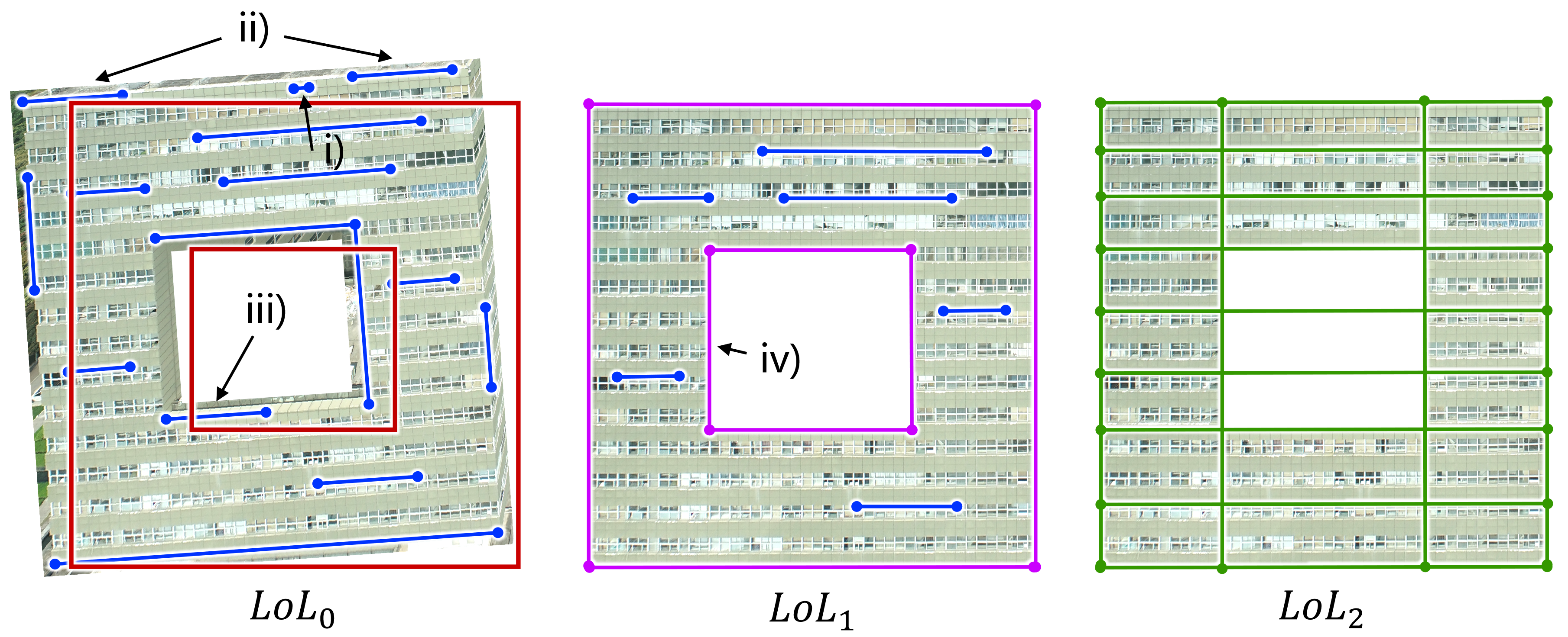
.
After registering image via rigid alignment, we obtain its which has higher accuracy than . However, the registered line segments still cannot well represent the polygon boundary. Our next step is to obtain which can maximally match .
We first measure the partial matching relationship of a line segment compared to a boundary edge considering:
![[Uncaptioned image]](/html/2309.11258/assets/x4.png)
a) , the angle between two lines. b) , the maximum point-to-line distance from end-points to another line. Moreover, it is useful in matching line segments with similar slopes and spatial distance, but large variances in length. c) , the level of non-overlap between and . To compute it, is first projected to to get . We compute based on four types of relationship between and after line projection, see the inset figure. In case 1 and 2, we assign infinity to . In case 3, is set to zero. A point projected on with end-points and can be denoted as . In the last case, for the end-point of locating outside ( or ), we calculate its distance to the end-points of and assign the minimum value to . with value of a)-c) smaller than given thresholds will be denoted as a boundary matching line .
The set of lines of are further refined by: i) eliminating tiny noisy matching any , ii) merging the set of lines matching the same into one single line segment, iii) extending and until they share a same end-point, if the matching boundary and of and are neighbors, and iv) connecting and whose matching boundary are and respectively, if the inserted can match whose neighbors are and . The above operations are illustrated in Fig. 8 and the refined are visualized in purple. The can serve as a guidance for texture stitching in Sec. 5.2.
.
Finally, we cluster all the line segments in to extract structural lines with a dynamic K-means algorithm, according to the slope and the distance from the image center to the line segment. After that, we can obtain to represent the structural layouts of facade components and to serve as a reference for later inpainting in Sec. 5.3. Until now, for each selected image, we obtain LoLs for different operators. Fig. 8 illustrates the LoLs from a facade image of Hitech.
5.2. Line-guided Texture Stitching
For each proxy polygon , we have obtained a subset of views along with their LoLs in previous steps. For simplicity, we denote the first selected image in as a reference image and the others as target images . To generate an enlarged texture map, we need to find the matching relationship between two images to stitch them together. Based on extracted LoLs, one solution is to find the correspondence between the lines (e.g., using LBD descriptor (Zhang and Koch, 2013)) by considering both image and geometry features. However, there exists plenty of repetitive patterns which make such pixel-based methods less effective. Therefore, we develop an algorithm for matching line segments by utilizing geometric information.
Due to the camera and geometry inaccuracy, there exists obvious texture-to-geometry displacement which increases the difficulty in accurate image local matching and stitching. We start by globally registering towards with a rigid transformation and several warping operators. Next, following the order of their insertion into , all the are sequentially deformed to match globally, then locally stitched to . The -th inserted image is denoted as . The stitching process is done in three steps: rigid alignment, line matching and texture warping.
Rigid alignment.
To reduce the large texture-to-geometry misalignment, each image is transformed toward the proxy boundary . Firstly, we extend each image with a margin of pixels and extract complete from the extended version. We compute the bounding box of and set to of the length of its diagonal. This can be observed in Fig. 8. Next, we convert all the endpoints of in into a source point cloud . We then convert the endpoints of into a target point cloud . A rigid transformation is calculated via ICP (Besl and McKay, 1992) to align toward . This rigid transformation is employed to transform and update .
Line segment matching.
We denote of as and as . For each line segment , it can be registered to line segment if satisfying: i) the angular distance is smaller than , ii) the point-to-line distance is closer than 10 pixels, and iii) the level of non-overlap is smaller than 100 pixels if . We denote as the set of all pairs of matched line segments between and .
Texture warping.
With the matched lines in , we can warp to while preserving the matched line segments. The warping of to shares the same process. Previous work (Jia et al., 2021) converts the transformation into a global line-guided mesh deformation problem. They rely on deforming the vertices of a grid-mesh uniformly sampled in the target image to maintain line structures by solving a global least-square energy function.
However, the global optimal deformation method may not guarantee the strict straightness of colinear line features in facade images.
![[Uncaptioned image]](/html/2309.11258/assets/images/adaptive-mesh.png)
In this work, we employ an adaptive-mesh data structure to explicitly maintain the line segments after warping. First, we construct a constrained Delaunay triangulation based on , keeping all the inserted segments as constraint edges, as shown in the right wrapped figure. Unlike uniformly sampling grid-mesh data structure, every basic element in our adaptive mesh encodes a meaningful geometric primitive in the target image, i.e., a corner point or a line segment. Based on this, all the vertices are deformed to new positions while satisfying the following two constraints:
-
•
The matched line segment pairs in are well aligned after the mesh deformation.
-
•
All the line segments in preserve straightness after the mesh deformation.
We search for the optimal deformation offset by embedding these two constraints and a normalization term into an energy minimization formulation:
| (5) |
represents the line-alignment term, which guarantees the alignment between all pairs of matched line segments in after deforming vertices by in the form of
| (6) |
where is the -th matched line segment in , and are end points of -th matched line segment in . Moreover, the line-preserving term denoted as ensures the straightness of each line segment in after mesh deformation by
| (7) |
where are end points of -th line segment in and is the normal vector of . The normalization term to prevent exaggerate deformation is defined as . , , and in Eq. 5 is set to 0.5, 0.5, and 0.025 in all experiments.
Instead of optimizing the vertex position via LSQM (Jia et al., 2021), we calculate the vertex offset by applying the conjugate gradient algorithm which is more stable and efficient. Unlike using the calculated vertex position to update enclosing grid vertices with bilinear interpolation (Jia et al., 2021), each line segment represents a linear feature of a facade component in our case. We directly apply the optimal vertex offsets to the end-points of lines for the preservation of linear features. There can appear topological issues of the updated mesh after that. Hence, we introduce a refinement step to address the topological issues such as line crossing and non-manifolds. Finally, with an affine transformation constructed by the refined vertices of adaptive mesh facet , each pixel inside the is warped to the new position . With the alignment and warping operators, all the visible regions are globally warped to and locally warped to forming an enlarged texture image for each proxy polygon .
5.3. Texture Optimization
Illumination adjustment.
Previous steps enable us to generate a texture map for each proxy polygon . Since is composed of patches extracted from various viewing directions, the brightness may be inconsistent across neighbouring patches. Assuming that the brightness distribution over the whole texture map should hold a specific pattern, we perform a histogram specification operation to improve the illumination consistency of in HSV color space. To be precise, we first calculate a distribution histogram of the channel on the non-overlapping region of and overlapping region of , respectively. Next, we match these two histograms and transfer the brightness of the overlapping region on to the non-overlapping region on .
Texture inpainting.
In practice, some regions in may not be observed by any of the selected views or covered with high-quality patches, leading to holes in the generated texture map. To reduce this visual artifacts, we need to fill the missing regions (referred to as masks) to generate a complete texture map. However, the arbitrary sizes and irregular shapes of the mask pose great challenges to previous inpainting methods (e.g., patch-based approaches (Barnes et al., 2009; Huang et al., 2014)). Inspired by the strong capability of diffusion model in generating semantic and geometric harmonious results, we employ a denoising diffusion probabilistic model called RePaint (Lugmayr et al., 2022) for free-form inpainting.
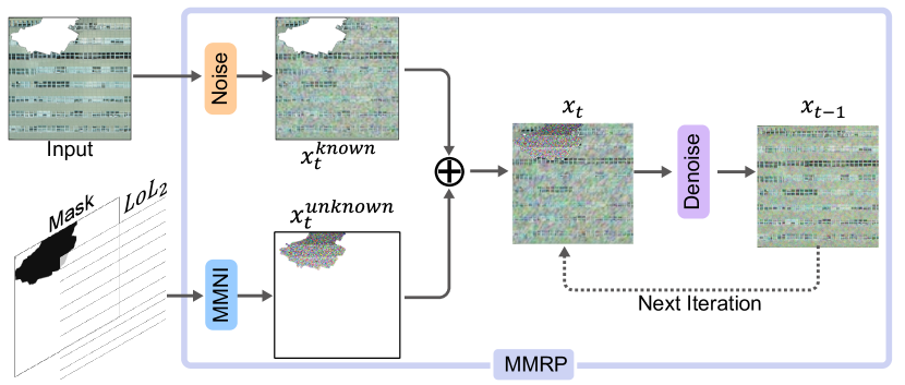
However, RePaint is still not robust enough to generate structurally consistent results for a large missing region. To alleviate this issue, we further introduce a line-guided version of RePaint called Multi-Mask RePaint model (MMRP) to preserve the geometric consistency. As shown in Fig. 9, the input of MMRP contains the mask, , and the texture to be completed. We then propose a multi-mask noise initialization (MMNI) component. Firstly, we compute the principal directions of the lines in by using principal component analysis (PCA). Our MMNI divides the unobserved region into several parts following the second max principal direction. As mentioned by Croitoru et al. (2023), the results will show better Frechet Inception Distance values and faster convergence with a mixture of Gaussian noises. Inspired by this observation, unlike the original RePaint that initializes the entire unobserved region with a single random Gaussian noise, we randomly initialize each divided part with a random Gaussian noise , where ranges from [0, 10], ranges from [1, 50]. The ranges are chosen from experimental results that deliver good performance.
After that, the parts initialized with multiple noises along with observed content are merged into one image, , which will be harmonized together into a new inpainting. With MMNI, our MMRP can increase the possibility of generating result that is more consistent with the observed region.
We find that the quality of training data is crucial for diffusion model to generate feasible results for a specific scenario, such as the architecture in our case. To adapt RePaint to our task, we create a TwinTex dataset and fine-tune Repaint which was originally trained on ImageNet (Russakovsky et al., 2015). Starting from high-resolution images collected with aerial drone covering outdoor architectural scenes, we first project each image to all its visible and extract the pixels inside the bounding box of visible regions. Each extracted image is then cropped to a set of images with the size of . Next, we remove the images with heavy blurring issues or containing a large portion of non-architectural contents (e.g., vegetation, human, scaffolds, etc) (Zhao et al., 2017). Our final TwinTex dataset (TwinTexSet) contains images of various scene components and building categories (school, office building, etc). Note that all the image regions with heavy blurring issue and extreme inclined angles have been removed from our data set. Note that there are some overlaps between the training and testing scenes. However, the TwinTex dataset contains the processed photos of 17 outdoor scenes, where we have rectified the photos, removed blurring regions and large non-architectural objects. After these processes, the training images and the test texture maps have no overlap. The missing regions in test images come from frustum-culling, visibility detection, or are not included in input photos. Therefore, the regions to be infilled never appear in the training images, thus never seen by the trained model in our tasks.
We make use of our TwinTex dataset to fine-tune the pre-trained RePaint model. The total training time is about 9 hours. We only need to pay the time cost for training once. For an image with high resolution, we will resize it to . And for an image with large missing area, we choose to scale it according to the largest dimension while preserving the image ratio. The resized image will be fed into MMRP to receive a semantic and geometric consistent inpainting. Finally, we upsample the resultant inpainting to the original size with a bi-linear interpolation operation. Please refer to the supplemental for more details and experimental results.
6. Results
To validate the proposed algorithm, we conduct a series of experiments on real-world scenes with varying building styles and functions. We first demonstrate the robustness of our approach and the effectiveness of each main ingredient through a stress test. Then, we evaluate our approach by comparing it against state-of-the-art texture mapping methods. Ablation studies are performed as well to show the effectiveness of our main technical ingredients (please refer to the supplemental material for the details). Texturing results by our method and manual work on proxy models at different levels of detail are also provided in the supplemental material to demonstrate the high quality of our generated texture maps. Our algorithm is implemented in C++ and also well-organized as a customized plug-in for Houdini. All the presented experimental results are obtained on a desktop computer equipped with an Intel i9-10900k processor with 3.0 GHz and 128 GB RAM. Note that the time cost for fine-tuning the RePaint model are not included in the statistics.
Dataset.
For the performance evaluation and comparisons, we carry out experiments on real-world scenes, including outdoor buildings, two indoor rooms and a man-made object. These scenes come from public sources (i.e., Library (Zhang et al., 2021), Hitech (Zhou et al., 2020), Polytech and ArtSci (Lin et al., 2022)), a handheld device (i.e., Machine Room, Lab, Cabinet), or are captured by a single-camera drone (i.e., Highrise, School, Center, CSSE, Sunshine Plaza, Hall, Center, Factory, Hisense, Bank, Apartment). Please refer to the supplemental material for detailed statistics on the photo collections and models. Then we use the commercial software RealityCapture222https://www.capturingreality.com/ (RC) to reconstruct the 3D high-precision models from the captured images. All the abstracted versions are either the 2.5D models for path planning (Zhou et al., 2020), or created by in-field modelers. All of the dense reconstructions and proxy models are utilized to demonstrate the performance of our algorithm.
6.1. Stress Test
We first evaluate the robustness of our approach on a complicated Hall example with 519 input views. This stress test is performed via randomly removing partial photos from the original photo set and feeding the rest views into our TwinTex. The textured proxies of Hall example generated with three different sets of remaining views are shown in Fig. 10. We also show the intermediate texture maps after each step, e.g., view selection, image stitching along with blending and texture inpainting.
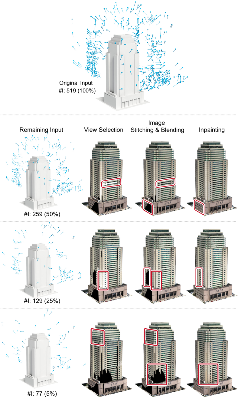

We randomly removed , and photos from the original set and made use of the remaining views to texture this proxy model. The textured proxies after view selection are generated by simply overlapping the projection of selected images following the reverse order of selection. As the number of photos in the remaining input decreased, our selection algorithm can still select high-quality photos from the input to maximally cover the proxy, as illustrated in the second column of Fig. 10. From the third column, we can see the texture maps after performing our stitching step and illumination adjustment exhibit higher geometric and photometric consistency. However, there appears larger missing regions as the number of remaining views decrease. We only use images to texture Hall example with facades (each plane has about photos to select from). All the missing regions are visualized with black pixels, as marked by the red boxes in the figure. The final texture maps visualized in the last column of Fig. 10 demonstrate the ability of our inpainting framework for creating geometrically and semantically consistent contents under very limited resource.
6.2. Comparison with Texturing Methods
In this subsection, we evaluate the quality of our generated texture maps by comparing them against RC and two competitive texturing generation frameworks, let there be color (LTBC) (Waechter et al., 2014) and patch based optimization (PBO) (Bi et al., 2017). We adopt the evaluation scheme proposed by Waechter et al. (2017) to compare the rendered image with the corresponding real image following a specific view from the input cameras. We select the ground truth photos for evaluation from the input excluding the photos for texturing. Two visual similarity metrics, namely the structural similarity index measure (SSIM) and learned perceptual image patch similarity (LPIPS) (Kastryulin et al., 2022), are adopted for quantitative evaluation.
Comparison with LTBC. We first compare our method with RC and LTBC on two examples. Note that LTBC selects the most suitable view for each facet by solving a Markov Random Field formulation and adjusting the pixel values along the boundary edges of adjacent patches to alleviate the seams. This strategy fails to texture large facets when there is no camera view observing the whole region of the facet. Thus, we subdivide the simplified coarse model and perform LTBC to generate texture maps for the corresponding subdivided mesh for a reasonable comparison.
| Scene | Method | Time (min) | ||
|---|---|---|---|---|
| Center | RC | 0.350 | 0.831 | 287.0 |
| LTBC | 0.354 | 0.836 | 4.4 | |
| Ours | 0.358 | 0.831 | 167.4 | |
| Artsci | RC | 0.346 | 0.883 | 320.9 |
| LTBC | 0.331 | 0.873 | 6.0 | |
| Ours | 0.348 | 0.877 | 256.1 |
| Scene | Method | Time | ||
|---|---|---|---|---|
| Library | RC | { 0.28, 0.28, 0.32 } | { 0.53, 0.60, 0.68 } | 383.6 |
| LTBC | { 0.29, 0.29, 0.34 } | { 0.54, 0.68, 0.68 } | 4.8 | |
| PBO | { 0.63, 0.45, 0.38 } | { 0.63, 0.67, 0.69 } | 810.7 | |
| Ours | { 0.46, 0.38, 0.36 } | { 0.28, 0.52, 0.66 } | 200.4 | |
| Bank | RC | { 0.25, 0.62, 0.26 } | { 0.43, 0.23, 0.54 } | 198.3 |
| LTBC | { 0.20, 0.52, 0.33 } | { 0.51, 0.37, 0.53 } | 6.4 | |
| PBO | { 0.25, 0.70, 0.27 } | { 0.43, 0.31, 0.57 } | 672.1 | |
| Ours | { 0.26, 0.63, 0.28 } | { 0.27, 0.18, 0.52 } | 174.5 |
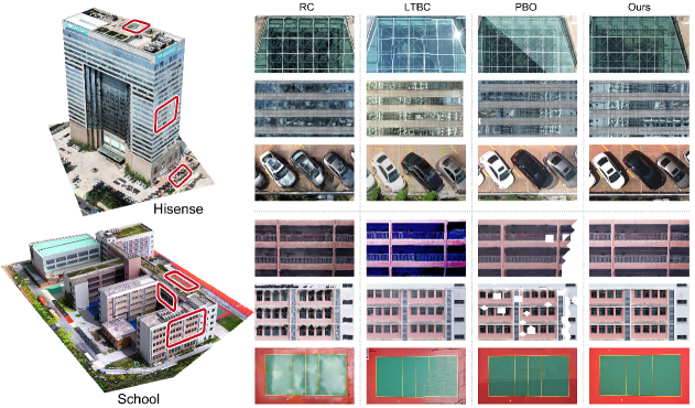
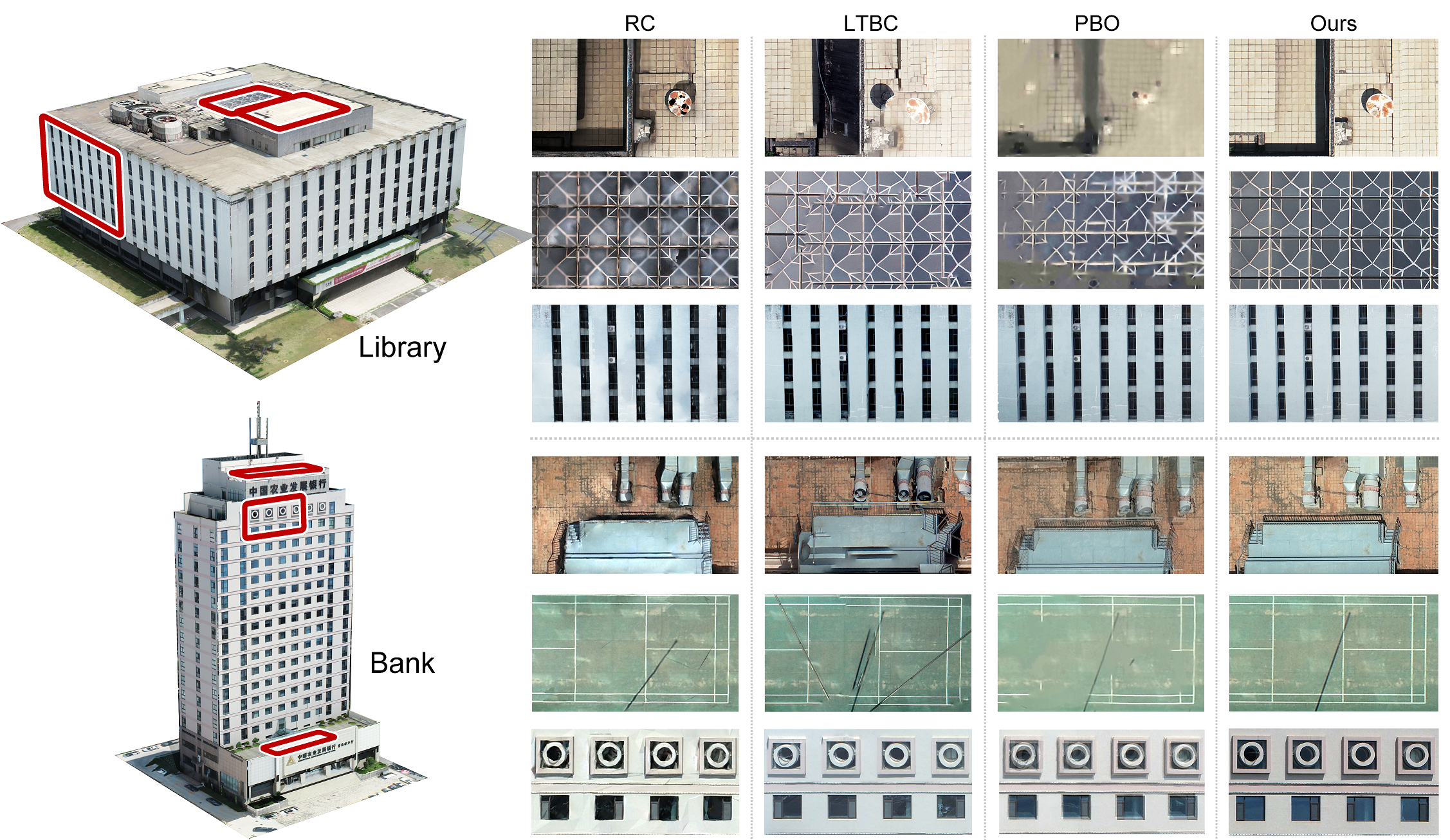
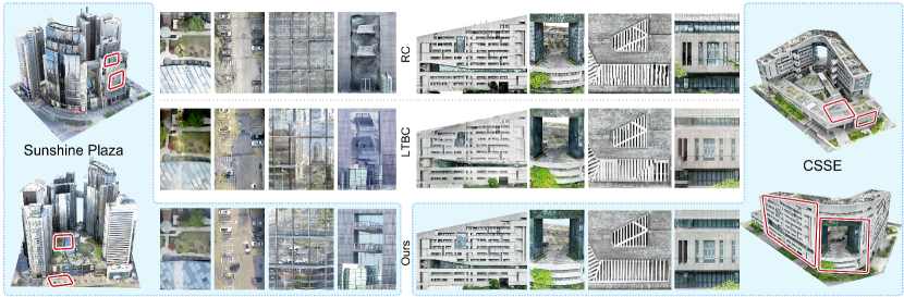
Fig. 11 shows the qualitative results on two abstracted models with sharp textures and structural features. First, we can observe that LTBC and RC are not able to produce satisfactory results for large-scale planar structures which are invisible for the input photos or with only low-quality pixels. In these cases, their texture maps show blurring and ghosting artifacts. By contrast, our method can fill large unobserved regions with geometrically and semantically consistent pixels.
Second, without the constraints on perspective consistency in view selection, LTBC failed in selecting photos with both consistent and front-parallel viewing directions, creating ”stretching” alike artifact and perspective inconsistency in the generated textures. The ”stretching” problem can be observed in the inset of the ArtSci building in Fig. 11 (first row, second column), which was caused by merging photos with large viewing angle variance. The perspective inconsistency can be observed in the insets of the Center example in Fig. 11 (first and third rows, second column). Unlike LTBC, our view selection strategy can pick out a very small set of perspective consistent and front-parallel photos as possible. Moreover, we introduced a smooth term considering the pixel-wise distance of each image pair. This helps select a set of photos with a higher level of photometric and content consistency, especially for filtering out occluders or dynamic instances (e.g., cars). The significant improvement can be observed in the Center example in Fig. 11 (second row) and ArtSci example in Fig. 11 (third row).
Furthermore, due to the lack of explicit constraints on the linear features of buildings, the texture generated by LTBC destroys geometric structures, making them suffer from serious seams and distortion effects. Our image stitching mechanism succeeds in preserving the straightness and completeness of the line segments by constructing an adaptive mesh taking the original geometric primitives as constraints. Next, large and duplicate texture patterns are also well maintained in our results. This is mainly because we select a suitable small subset of camera views for each planar shape instead of each facet. This strategy guarantees that each selected view is used to texture the current plane as much as possible.
The quantitative comparison results are given in Table 1. In most of the cases, the rendered views of our textured model can deliver better SSIM and LPIPS scores. Please refer to the supplemental material for the overall views of the above two examples.
Comparison with PBO. Next, we perform comparison with PBO333https://github.com/yanqingan/EAGLE-TextureMapping and report SSIM and LPIPS as well on four more architectural scenes. We first tried to globally compare the similarity of rendering views on the entire building with real photos. However, PBO requires an extremely large amount of time/storage given just several high-resolution images as input. Remember that our target is to retain the quality of the inputs, one way to address the issues is to decrease the number of input photos. This can produce other problems such as missing contents since no pixels can cover some of the regions. It is crucial to provide key views with high quality to the PBO in this scenario. Hence, we locally perform the comparison to PBO using three planes per example. To this end, we fed PBO with the set of views selected by our algorithm for the planar polygons involved in the comparison. Considering the nature of patch-based optimization, for a fair qualitative comparison, we use the subdivided mesh prepared for LTBC as the input to PBO as well. Fig. 12 shows the texturing results of RC, LTBC, PBO and ours. The comparison shows that given the same set of selected views, PBO can generate a texture with good quality in most cases which also proves the effectiveness of our view selection algorithm. However, the results of PBO have obvious blurring issue and line distortion artifact compared to the real photos. There are also some optimization failures of PBO which cause missing textures for the subdivided triangles. In comparison, our stitching and optimization frameworks can preserve clear line features and retain the original structure while we are able to inpaint missing regions.
Quantitative results are listed in Table 2. Since SSIM is by nature less sensitive to blurring issues and possibly gives higher scores to images with such artifacts (Zhang et al., 2018), the texture with the regional blurring problem could have higher scores. This phenomenon can be observed in some views per each example. Meanwhile, LPIPS is designed to match human perception and yield better scores for images with higher level of coherence. Note that the recorded time cost for PBO does not include view selection or is not for texturing the entire proxy although it is relatively long.
6.3. Analysis of Generalization Ability
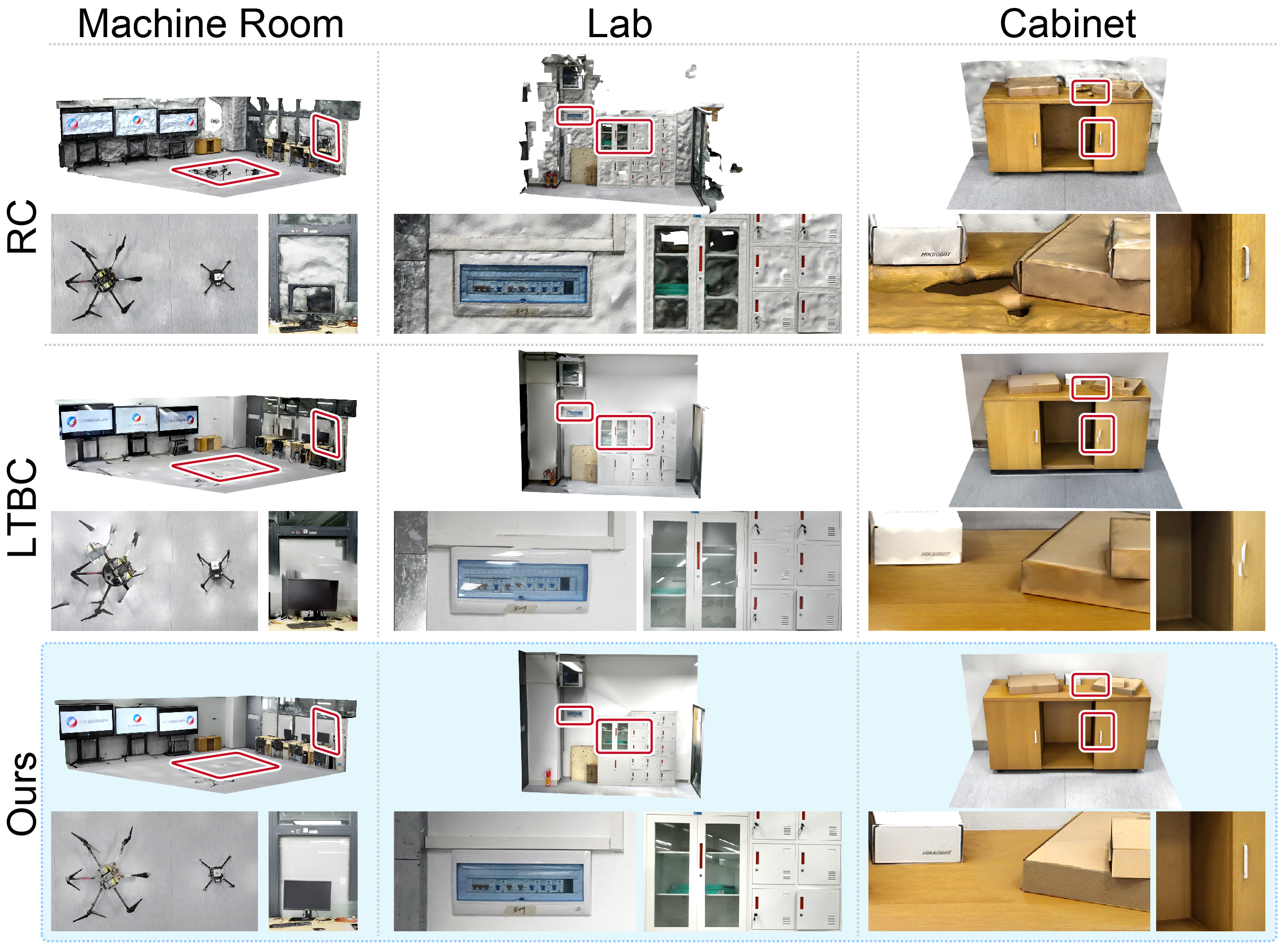
In this subsection, we discuss the results of our method applied to more diverse scenes. First, we conduct experiments on several challenging urban scenes that contain curve surfaces, facades with non-linear features, and facades with a lot of reflection, as shown in Fig. 13. Then we present the texturing results on two indoor scenes and one man-made object in Fig. 14, which are different scenarios from buildings. Note there exists only one fire extinguisher in the Lab scene. Although it has been moved during the photos collection process, our method still perfectly keeps its location where it has been placed in most photos.
To better understand the superiority of our TwinTex, we conduct comparisons with previous methods as well. From the figures we can see that our approach can still generate high-fidelity textures for the challenging buildings, and can be naturally extended to texture coarse piece-wise planar models in other scenarios. The visual comparisons further suggest that the textures generated by our approach have several significant advantages over previous methods: i) closer to real photos with perspective consistency and harmonic illumination, ii) contain rarely border misalignment, distortion, blurring and seaming artifacts resulting from inaccurate camera parameters, iii) contain rarely ghosting effects resulting from dynamic instances, iv) preserve geometric details better, and v) fill the missing regions with geometrically and semantically consistent contents.
7. Conclusion and Future Work
In this work, we proposed a plane-based and geometry-aware texture generation method. Our target is to produce high-resolution texture maps for piece-wise planar architectural proxy models which were abstracted from dense 3D reconstructions. Our main technical contributions consist in: i) A greedy algorithm to select a set of views that are most suitable for texturing each planar shape; Both perspective and photometric qualities are considered in this algorithm. ii) An image stitching methodology that can stitch the selected views to an enlarged texture map, preserving the local and global linear geometric primitives based on an adaptive-mesh data structure; iii) An improved diffusion probabilistic model that fine-tuned with our created TwinTexSet to inpaint unobserved texture region with semantically and geometrically coherent pixels; iv) A customized texturing tool plugged in a widely used graphical engine. Experimental results show that our algorithm outperforms state-of-the-art facet-based texturing methods in the generation of realistic and high-resolution texture maps in a reasonable time.
Limitations and future work. Our system still has several limitations. First, although we significantly refined the extracted line segments, the line-guided scheme still relies on the quality of the line extraction algorithm. One possible solution is to consider camera information as well or make use of reconstructed 3D lines. Second, our plane-based texture generation method processes each planar shape independently, which does not take their mutual relationship into consideration. Fig. 15 (left) shows such an example where global alignment of linear features between adjacent planes is not achieved. Note we here choose a zoom-in view with the most obvious misalignment among given buildings to clearly show this issue. The other examples may also exhibit tiny misalignments. Third, we may fail to successfully perform inpainting for a reflected facade which lacks of coherent structures and clear content, making it even hard for a human to infer the missing region, see Fig. 15 (right). Finally, the processing time can be further improved with parallel processing. We will incorporate these issues in our future pipeline.
Acknowledgments
We thank the reviewers for their constructive comments. This work was supported in parts by NSFC (U21B2023, U2001206, U22B2034, 62172416, 62302313), DEGP Innovation Team (2022KCXTD025), and Shenzhen Science and Technology Program (KQTD202108110900440 03, RCJC20200714114435012, JCYJ20210324120213036).
References
- (1)
- Baatz et al. (2022) Hendrik Baatz, Jonathan Granskog, Marios Papas, Fabrice Rousselle, and Jan Novák. 2022. NeRF-Tex: Neural Reflectance Field Textures. Comp. Graph. Forum 41, 6 (2022), 287–301.
- Barnes et al. (2009) Connelly Barnes, Eli Shechtman, Adam Finkelstein, and Dan B Goldman. 2009. PatchMatch: A randomized correspondence algorithm for structural image editing. ACM Trans. Graph. 28, 3 (2009), 24:1–24:11.
- Bauchet and Lafarge (2020) Jean-Philippe Bauchet and Florent Lafarge. 2020. Kinetic shape reconstruction. ACM Trans. Graph. 39, 5 (2020), 156:1–156:14.
- Bernardini et al. (2001) Fausto Bernardini, Ioana M. Martin, and Holly Rushmeier. 2001. High-quality texture reconstruction from multiple scans. IEEE Trans. on Vis. and Comp. Graph. 7, 4 (2001), 318–332.
- Besl and McKay (1992) Paul J Besl and Neil D McKay. 1992. Method for registration of 3-D shapes. In Sensor fusion IV: control paradigms and data structures, Vol. 1611. 586–606.
- Bi et al. (2017) Sai Bi, Nima Khademi Kalantari, and Ravi Ramamoorthi. 2017. Patch-based optimization for image-based texture mapping. ACM Trans. Graph. (SIGGRAPH) 36, 4 (2017), 106:1–106:11.
- Bouzas et al. (2020) Vasileios Bouzas, Hugo Ledoux, and Liangliang Nan. 2020. Structure-aware building mesh polygonization. ISPRS Journal of Photogrammetry and Remote Sensing 167 (2020), 432–442.
- Boykov et al. (2001) Yuri Boykov, Olga Veksler, and Ramin Zabih. 2001. Fast approximate energy minimization via graph cuts. IEEE Trans. Pattern Anal. Mach. Intell. 23, 11 (2001), 1222–1239.
- Brown and Lowe (2007) Matthew Brown and David G Lowe. 2007. Automatic panoramic image stitching using invariant features. Int. Journal of Computer Vision 74, 1 (2007), 59–73.
- Callieri et al. (2008) Marco Callieri, Paolo Cignoni, Massimiliano Corsini, and Roberto Scopigno. 2008. Masked photo blending: Mapping dense photographic data set on high-resolution sampled 3D models. Computers & Graphics 32, 4 (2008), 464–473.
- Ceylan et al. (2012) Duygu Ceylan, Niloy J Mitra, Hao Li, Thibaut Weise, and Mark Pauly. 2012. Factored facade acquisition using symmetric line arrangements. Comp. Graph. Forum (Proc. EUROGRAPHICS) 31, 2pt3 (2012), 671–680.
- Ceylan et al. (2014) Duygu Ceylan, Niloy J Mitra, Youyi Zheng, and Mark Pauly. 2014. Coupled structure-from-motion and 3D symmetry detection for urban facades. ACM Trans. Graph. 33, 1 (2014), 1–15.
- Chang et al. (2014) Che-Han Chang, Yoichi Sato, and Yung-Yu Chuang. 2014. Shape-preserving half-projective warps for image stitching. In IEEE Computer Vision and Pattern Recognition (CVPR). 3254–3261.
- Cohen-Steiner et al. (2004) David Cohen-Steiner, Pierre Alliez, and Mathieu Desbrun. 2004. Variational shape approximation. In Proc. ACM SIGGRAPH. 905–914.
- Croitoru et al. (2023) Florinel-Alin Croitoru, Vlad Hondru, Radu Tudor Ionescu, and Mubarak Shah. 2023. Diffusion models in vision: A survey. IEEE Trans. Pattern Anal. Mach. Intell. (2023).
- Debevec et al. (1998) Paul Debevec, Yizhou Yu, and George Borshukov. 1998. Efficient view-dependent image-based rendering with projective texture-mapping. In Eurographics Workshop on Rendering Techniques. 105–116.
- Debevec et al. (1996) Paul E Debevec, Camillo J Taylor, and Jitendra Malik. 1996. Modeling and rendering architecture from photographs: A hybrid geometry-and image-based approach. In Proc. ACM SIGGRAPH. 11–20.
- Dhariwal and Nichol (2021) Prafulla Dhariwal and Alexander Nichol. 2021. Diffusion models beat gans on image synthesis. Proc. International Conference on Neural Information Processing Systems 34 (2021), 8780–8794.
- Elharrouss et al. (2020) Omar Elharrouss, Noor Almaadeed, Somaya Al-Maadeed, and Younes Akbari. 2020. Image Inpainting: A Review. Neural Process. Letters 51, 2 (2020), 2007–2028.
- Fang and Lafarge (2020) Hao Fang and Florent Lafarge. 2020. Connect-and-Slice: an hybrid approach for reconstructing 3D objects. In IEEE Computer Vision and Pattern Recognition (CVPR). 13490–13498.
- Fu et al. (2020) Yanping Fu, Qingan Yan, Jie Liao, and Chunxia Xiao. 2020. Joint texture and geometry optimization for RGB-D reconstruction. In IEEE Computer Vision and Pattern Recognition (CVPR). 5950–5959.
- Fu et al. (2018) Yanping Fu, Qingan Yan, Long Yang, Jie Liao, and Chunxia Xiao. 2018. Texture mapping for 3d reconstruction with RGB-D sensor. In IEEE Computer Vision and Pattern Recognition (CVPR). 4645–4653.
- Gal et al. (2010) Ran Gal, Yonatan Wexler, Eyal Ofek, Hugues Hoppe, and Daniel Cohen-Or. 2010. Seamless montage for texturing models. Comp. Graph. Forum 29, 2 (2010), 479–486.
- Gao et al. (2011) Junhong Gao, Seon Joo Kim, and Michael S Brown. 2011. Constructing image panoramas using dual-homography warping. In IEEE Computer Vision and Pattern Recognition (CVPR). 49–56.
- Garcia-Dorado et al. (2013) Ignacio Garcia-Dorado, Ilke Demir, and Daniel G Aliaga. 2013. Automatic urban modeling using volumetric reconstruction with surface graph cuts. Computers & Graphics 37, 7 (2013), 896–910.
- Garland and Heckbert (1997) Michael Garland and Paul S Heckbert. 1997. Surface simplification using quadric error metrics. In Proc. ACM SIGGRAPH. 209–216.
- Georgiou et al. (2021) Yiangos Georgiou, Melinos Averkiou, Tom Kelly, and Evangelos Kalogerakis. 2021. Projective Urban Texturing. In International Conference on 3D Vision (3DV). 1034–1043.
- Guillemot and Meur (2014) Christine Guillemot and Olivier Le Meur. 2014. Image Inpainting: Overview and Recent Advances. IEEE Signal Processing Magazine 31, 1 (2014), 127–144.
- Guo et al. (2022) Jianwei Guo, Yanchao Liu, Xin Song, Haoyu Liu, Xiaopeng Zhang, and Zhanglin Cheng. 2022. Line-Based 3D Building Abstraction and Polygonal Surface Reconstruction From Images. IEEE Trans. on Vis. and Comp. Graph. (2022), 1–15.
- Huang et al. (2017) Jingwei Huang, Angela Dai, Leonidas J Guibas, and Matthias Nießner. 2017. 3Dlite: towards commodity 3D scanning for content creation. ACM Trans. Graph. (SIGGRAPH Asia) 36, 6 (2017), 203:1–203:14.
- Huang et al. (2014) Jia-Bin Huang, Sing Bing Kang, Narendra Ahuja, and Johannes Kopf. 2014. Image completion using planar structure guidance. ACM Trans. Graph. (SIGGRAPH) 33, 4 (2014), 129:1–129:10.
- Jam et al. (2021) Jireh Jam, Connah Kendrick, Kevin Walker, Vincent Drouard, Jison Gee-Sern Hsu, and Moi Hoon Yap. 2021. A comprehensive review of past and present image inpainting methods. Computer vision and image understanding 203 (2021), 103147.
- Jia et al. (2021) Qi Jia, ZhengJun Li, Xin Fan, Haotian Zhao, Shiyu Teng, Xinchen Ye, and Longin Jan Latecki. 2021. Leveraging line-point consistence to preserve structures for wide parallax image stitching. In IEEE Computer Vision and Pattern Recognition (CVPR). 12186–12195.
- Kastryulin et al. (2022) Sergey Kastryulin, Jamil Zakirov, Denis Prokopenko, and Dmitry V Dylov. 2022. PyTorch Image Quality: Metrics for Image Quality Assessment. arXiv preprint arXiv:2208.14818 (2022).
- Kelly et al. (2018) Tom Kelly, Paul Guerrero, Anthony Steed, Peter Wonka, and Niloy J. Mitra. 2018. FrankenGAN: Guided Detail Synthesis for Building Mass Models Using Style-Synchonized GANs. ACM Trans. Graph. (SIGGRAPH Asia) 37, 6 (2018), 216:1–216:14.
- Kwatra et al. (2003) Vivek Kwatra, Arno Schödl, Irfan Essa, Greg Turk, and Aaron Bobick. 2003. Graphcut textures: Image and video synthesis using graph cuts. ACM Trans. Graph. 22, 3 (2003), 277–286.
- Lee and Sim (2020) Kyu-Yul Lee and Jae-Young Sim. 2020. Warping residual based image stitching for large parallax. In IEEE Computer Vision and Pattern Recognition (CVPR). 8198–8206.
- Lempitsky and Ivanov (2007) Victor Lempitsky and Denis Ivanov. 2007. Seamless mosaicing of image-based texture maps. In IEEE Computer Vision and Pattern Recognition (CVPR). 1–6.
- Li et al. (2017) Nan Li, Yifang Xu, and Chao Wang. 2017. Quasi-homography warps in image stitching. IEEE Trans. Multimedia 20, 6 (2017), 1365–1375.
- Li et al. (2015) Shiwei Li, Lu Yuan, Jian Sun, and Long Quan. 2015. Dual-feature warping-based motion model estimation. In IEEE International Conference on Computer Vision (ICCV). 4283–4291.
- Liao and Li (2019) Tianli Liao and Nan Li. 2019. Single-perspective warps in natural image stitching. IEEE Trans. Image Process. 29 (2019), 724–735.
- Lin et al. (2015) Chung-Ching Lin, Sharathchandra U Pankanti, Karthikeyan Natesan Ramamurthy, and Aleksandr Y Aravkin. 2015. Adaptive as-natural-as-possible image stitching. In IEEE Computer Vision and Pattern Recognition (CVPR). 1155–1163.
- Lin et al. (2022) Liqiang Lin, Yilin Liu, Yue Hu, Xingguang Yan, Ke Xie, and Hui Huang. 2022. Capturing, Reconstructing, and Simulating: the UrbanScene3D Dataset. In European Conference on Computer Vision (ECCV). 93–109.
- Lin et al. (2011) Wen-Yan Lin, Siying Liu, Yasuyuki Matsushita, Tian-Tsong Ng, and Loong-Fah Cheong. 2011. Smoothly varying affine stitching. In IEEE Computer Vision and Pattern Recognition (CVPR). 345–352.
- Lugmayr et al. (2022) Andreas Lugmayr, Martin Danelljan, Andres Romero, Fisher Yu, Radu Timofte, and Luc Van Gool. 2022. Repaint: Inpainting using denoising diffusion probabilistic models. In IEEE Computer Vision and Pattern Recognition (CVPR). 11461–11471.
- Maier et al. (2017) Robert Maier, Kihwan Kim, Daniel Cremers, Jan Kautz, and Matthias Nießner. 2017. Intrinsic3D: High-quality 3D reconstruction by joint appearance and geometry optimization with spatially-varying lighting. In IEEE International Conference on Computer Vision (ICCV). 3114–3122.
- Mehta and Bhirud (2011) Jalpa D Mehta and SG Bhirud. 2011. Image stitching techniques. In Thinkquest~ 2010: Proceedings of the First International Conference on Contours of Computing Technology. 74–80.
- Metzer et al. (2022) Gal Metzer, Elad Richardson, Or Patashnik, Raja Giryes, and Daniel Cohen-Or. 2022. Latent-NeRF for Shape-Guided Generation of 3D Shapes and Textures. arXiv preprint arXiv:2211.07600 (2022).
- Monszpart et al. (2015) Aron Monszpart, Nicolas Mellado, Gabriel J Brostow, and Niloy J Mitra. 2015. RAPter: rebuilding man-made scenes with regular arrangements of planes. ACM Trans. Graph. (SIGGRAPH) 34, 4 (2015), 103:1–103:12.
- Müller et al. (2022) Thomas Müller, Alex Evans, Christoph Schied, and Alexander Keller. 2022. Instant Neural Graphics Primitives with a Multiresolution Hash Encoding. ACM Trans. Graph. (SIGGRAPH) 41, 4 (2022), 102:1–102:15.
- Musialski et al. (2010) Przemyslaw Musialski, Christian Luksch, Michael Schwärzler, Matthias Buchetics, Stefan Maierhofer, and Werner Purgathofer. 2010. Interactive Multi-View Facade Image Editing.. In Vision, Modeling, and Visualization. 131–138.
- Musialski et al. (2013) Przemyslaw Musialski, Peter Wonka, Daniel G Aliaga, Michael Wimmer, Luc Van Gool, and Werner Purgathofer. 2013. A survey of urban reconstruction. Comp. Graph. Forum 32, 6 (2013), 146–177.
- Nan and Wonka (2017) Liangliang Nan and Peter Wonka. 2017. PolyFit: Polygonal surface reconstruction from point clouds. In IEEE International Conference on Computer Vision (ICCV). 2353–2361.
- Pan et al. (2022) Shanshan Pan, Jiahui Lv, Hao Fang, and Hui Huang. 2022. Efficient and robust 3D structure-aware reconstruction. Journal of Image and Graphics 27, 2 (2022), 421–434.
- Pérez et al. (2003) Patrick Pérez, Michel Gangnet, and Andrew Blake. 2003. Poisson image editing. In Proc. ACM SIGGRAPH. 313–318.
- Rojas et al. (2020) David Josué Barrientos Rojas, Bruno José Torres Fernandes, and Sergio Murilo Maciel Fernandes. 2020. A Review on Image Inpainting Techniques and Datasets. In SIBGRAPI Conference on Graphics, Patterns and Images. 240–247.
- Russakovsky et al. (2015) Olga Russakovsky, Jia Deng, Hao Su, Jonathan Krause, Sanjeev Satheesh, Sean Ma, Zhiheng Huang, Andrej Karpathy, Aditya Khosla, Michael Bernstein, et al. 2015. Imagenet large scale visual recognition challenge. Int. Journal of Computer Vision 115, 3 (2015), 211–252.
- Salinas et al. (2015) David Salinas, Florent Lafarge, and Pierre Alliez. 2015. Structure-aware mesh decimation. Comp. Graph. Forum 34, 6 (2015), 211–227.
- Sinha et al. (2008) Sudipta N Sinha, Drew Steedly, Richard Szeliski, Maneesh Agrawala, and Marc Pollefeys. 2008. Interactive 3D architectural modeling from unordered photo collections. ACM Trans. Graph. 27, 5 (2008), 159:1–159:10.
- Smith et al. (2018) Neil Smith, Nils Moehrle, Michael Goesele, and Wolfgang Heidrich. 2018. Aerial Path Planning for Urban Scene Reconstruction: A Continuous Optimization Method and Benchmark. ACM Trans. Graph. (SIGGRAPH Asia) 37, 6 (2018), 183:1–183:15.
- Suárez et al. (2022) Iago Suárez, José M Buenaposada, and Luis Baumela. 2022. ELSED: Enhanced line SEgment drawing. Pattern Recognition 127 (2022), 108619.
- Szeliski et al. (2007) Richard Szeliski et al. 2007. Image alignment and stitching: A tutorial. Foundations and Trends® in Computer Graphics and Vision 2, 1 (2007), 1–104.
- Verdie et al. (2015) Yannick Verdie, Florent Lafarge, and Pierre Alliez. 2015. LOD generation for urban scenes. ACM Trans. Graph. 34, 3 (2015), 30:1–30:14.
- Waechter et al. (2017) Michael Waechter, Mate Beljan, Simon Fuhrmann, Nils Moehrle, Johannes Kopf, and Michael Goesele. 2017. Virtual Rephotography: Novel View Prediction Error for 3D Reconstruction. ACM Trans. Graph. 36, 1, Article 8 (2017), 11 pages.
- Waechter et al. (2014) Michael Waechter, Nils Moehrle, and Michael Goesele. 2014. Let there be color! Large-scale texturing of 3D reconstructions. In European Conference on Computer Vision (ECCV). 836–850.
- Wang et al. (2018) Bin Wang, Pan Pan, Qinjie Xiao, Likang Luo, Xiaofeng Ren, Rong Jin, and Xiaogang Jin. 2018. Seamless Color Mapping for 3D Reconstruction with Consumer-Grade Scanning Devices. In European Conference on Computer Vision (ECCV) Workshops. 633–648.
- Wang and Guo (2018) Chao Wang and Xiaohu Guo. 2018. Plane-based optimization of geometry and texture for RGB-D reconstruction of indoor scenes. In International Conference on 3D Vision (3DV). 533–541.
- Xiang et al. (2018) Tian-Zhu Xiang, Gui-Song Xia, Xiang Bai, and Liangpei Zhang. 2018. Image stitching by line-guided local warping with global similarity constraint. Pattern recognition 83 (2018), 481–497.
- Yuksel et al. (2019) Cem Yuksel, Sylvain Lefebvre, and Marco Tarini. 2019. Rethinking texture mapping. Comp. Graph. Forum 38, 2 (2019), 535–551.
- Zaragoza et al. (2013) Julio Zaragoza, Tat-Jun Chin, Michael S Brown, and David Suter. 2013. As-projective-as-possible image stitching with moving DLT. In IEEE Computer Vision and Pattern Recognition (CVPR). 2339–2346.
- Zhang et al. (2016) Guofeng Zhang, Yi He, Weifeng Chen, Jiaya Jia, and Hujun Bao. 2016. Multi-viewpoint panorama construction with wide-baseline images. IEEE Trans. Image Process. 25, 7 (2016), 3099–3111.
- Zhang et al. (2021) Han Zhang, Yucong Yao, Ke Xie, Chi-Wing Fu, Hao Zhang, and Hui Huang. 2021. Continuous Aerial Path Planning for 3D Urban Scene Reconstruction. ACM Trans. Graph. (SIGGRAPH Asia) 40, 6 (2021), 225:1–225:15.
- Zhang and Koch (2013) Lilian Zhang and Reinhard Koch. 2013. An efficient and robust line segment matching approach based on LBD descriptor and pairwise geometric consistency. Journal of Visual Communication and Image Representation 24, 7 (2013), 794–805.
- Zhang et al. (2018) Richard Zhang, Phillip Isola, Alexei A Efros, Eli Shechtman, and Oliver Wang. 2018. The unreasonable effectiveness of deep features as a perceptual metric. In IEEE Computer Vision and Pattern Recognition (CVPR). 586–595.
- Zhao et al. (2017) Hengshuang Zhao, Jianping Shi, Xiaojuan Qi, Xiaogang Wang, and Jiaya Jia. 2017. Pyramid scene parsing network. In IEEE Computer Vision and Pattern Recognition (CVPR). 2881–2890.
- Zhou and Koltun (2014) Qian-Yi Zhou and Vladlen Koltun. 2014. Color map optimization for 3D reconstruction with consumer depth cameras. ACM Trans. Graph. (SIGGRAPH) 33, 4 (2014), 155:1–155:10.
- Zhou et al. (2020) Xiaohui Zhou, Ke Xie, Kai Huang, Yilin Liu, Yang Zhou, Minglun Gong, and Hui Huang. 2020. Offsite Aerial Path Planning for Efficient Urban Scene Reconstruction. ACM Trans. Graph. (SIGGRAPH Asia) 39, 6 (2020), 192:1–192:16.