MS-GWaM: A 3-dimensional transient gravity wave parametrization for atmospheric models

Abstract

Parametrizations for internal gravity waves in atmospheric models are traditionally subject to a number of simplifications. Most notably, they rely on both neglecting wave propagation and advection in the horizontal direction (single-column assumption) and an instantaneous balance in the vertical direction (steady-state assumption). While these simplifications are well justified to cover some essential dynamic effects and keep the computational effort small it has been shown that both mechanisms are potentially significant. In particular, the recently introduced Multiscale Gravity Wave Model (MS-GWaM) successfully applied ray-tracing methods in a novel type of transient but columnar internal gravity wave parameterization (MS-GWaM-1D). We extend this concept to a three-dimensional version of the parameterization (MS-GWaM-3D) to simulate subgrid-scale non-orographic internal gravity waves. The resulting global wave model—implemented into the weather-forecast and climate code ICON—contains three-dimensional transient propagation with accurate flux calculations, a latitude-dependent background source, and convectively generated waves. MS-GWaM-3D helps reproducing expected temperature and wind patterns in the mesopause region in the climatological zonal mean state and thus proves a viable IGW parameterization. Analyzing the global wave action budget, we find that horizontal wave propagation is as important as vertical wave propagation. The corresponding wave refraction includes previously missing but well-known effects such as wave refraction into the polar jet streams. On a global scale, three-dimensional wave refraction leads to a horizontal flow-dependent redistribution of waves such that the structures of the zonal mean wave drag and consequently the zonal mean winds are modified.

This Work has been submitted to the Journal of Atmospheric Sciences. Copyright in this Work may be transferred without further notice.

1 Introduction

Internal gravity waves (IGWs) play a significant role in distributing energy and momentum throughout the atmosphere. Being generated through the perturbation of balanced flow states in stratified environments (e.g. convection, flow over topography, flow instabilities, wave turbulence, etc.) they may propagate over large distances and deposit their energy, generate turbulence and modify the mean-flow dynamics in general far away from their source (Fritts and Alexander, 2003; Alexander et al., 2010; Sutherland, 2010; Nappo, 2013; Williams et al., 2017; Sutherland et al., 2019; Achatz, 2022). While propagating they may exchange energy among themselves, transiently interact with mean flows, or influence the transport of chemical species. Even though their generation regions are mostly located in the troposphere, their effects are strongest in the middle atmosphere (Lindzen, 1981; Kim et al., 2003). However, these major effects may couple to and thus impact for instance tropospheric weather patterns or climate conditions (Scaife et al., 2005, 2012).

In state-of-the-art general circulation models (GCMs) or numerical weather prediction (NWP) models gravity waves are only partially resolved and thus need parameterization (e.g. Kim et al., 2003; Holt et al., 2016). Even when entering the global kilometer-resolving regime their effects are not entirely represented (Stephan et al., 2022). IGW parameterizations commonly rely on WKBJ theories (Bretherton, 1966; Grimshaw, 1975; Achatz et al., 2017), incorporating some major simplifications (Lindzen, 1981; Medvedev and Klaassen, 1995; Warner and McIntyre, 1996; Hines, 1997b, a; Lott and Miller, 1997; Alexander and Dunkerton, 1999; Scinocca, 2003; Orr et al., 2010; Lott and Guez, 2013). Most notably there are three assumptions that are usually made and shall be considered in this work. Firstly, local horizontal homogeneity is assumed in the so-called single-column approximation, i.e. horizontal gradients of the resolved flow are neglected, which leads horizontal wavenumbers to be invariant during propagation. Furthermore, responses of the resolved flow due to the horizontal finiteness of an IGW field are neglected. Secondly, a steady-state assumption is adopted such that IGWs instantly propagate through the atmosphere, leading to a neglect of all transient propagation effects. Thirdly, it is commonly assumed that the resolved flow is (approximately) in hydrostatic and geostrophic balance, implying a reduced formula for the resolved-flow response to IGWs. In the extratropics, this can lead to significant modifications in the IGW forcing when the flow is imbalanced.

Recent investigations have shown that all of the mentioned effects can have important impacts on modeled flows (Sato et al., 2009; Bölöni et al., 2016; Ehard et al., 2017; Wei et al., 2019), and several studies have successfully relaxed some of the simplifications (e.g. Muraschko et al., 2015; Wilhelm et al., 2018; Quinn et al., 2020). In particular, Bölöni et al. (2021) and Kim et al. (2021) presented a novel Lagrangian IGW parameterization, the Multi-Scale Gravity-Wave Model (MS-GWaM). It is built on a weakly non-linear WKBJ theory including transient wave-mean flow interactions. The model has been implemented in a single-column mode into a state-of-the-art weather forecast and climate code. It will therefore be referred to as MS-GWaM-1D throughout this manuscript. Here, we present MS-GWaM-3D, an extension of MS-GWaM-1D, which models the full 3D transient propagation of IGWs and their forcing of the general (cf. balanced) resolved flow. Ultimately, we aim to improve the representation of the parameterized IGW processes while keeping simulations numerically efficient.

This paper is structured as follows. First, a brief recapitulation of the underlying WKBJ theory for transient, 3-dimensional IGWs (Sec. 2) is presented. It is then followed by the description of the employed ray tracing techniques (Sec. 3). Lastly, results from simulations with MS-GWaM-3D (Sec. 4) are visualized and discussed. The manuscript then closes with some concluding remarks on the achievements and challenges of raytracing parameterization (Sec. 5).

2 Nonlinear, 3-dimensional and transient internal gravity waves

Albeit generally 3-dimensional and transient, internal gravity waves are commonly parameterized using both the single-column and the steady-state approximations. Here we attempt to relax both these assumptions and build a 3-dimensional and transient parameterization. The description of internal gravity waves in such a system is summarized in the following.

2.1 Wave evolution

We follow the analysis of Bretherton (1966); Grimshaw (1974); Hasha et al. (2008); Achatz et al. (2017); Achatz (2022) and summarize the Bretherton-Grimshaw modulation equations for a quasi-monochromatic wave train on a sphere. The governing equations are the compressible Euler equations as explained in Achatz et al. (2017). The presentation in these theories is extended by the inclusion of the atmospheric density scale height, so as to improve the realism in the non-hydrostatic regime, especially in the course of vertical reflection. Hence, we consider the well-known dispersion relation,

$$\omega(\bm{r},t) =\Omega(\bm{r},t,\bm{k})$$

$$=\bm{k}\cdot\bm{U}\pm\sqrt{\frac{f^{2}(k_{r}^{2}+\Gamma^{2})+N^{2}(k_{\lambda}^{2}+k_{\phi}^{2})}{K^{2}}},$$ (1)

with the position vector, $\bm{r}=\lambda\bm{e}_{\lambda}+\phi\bm{e}_{\phi}+r\bm{e}_{r}$, and the wave vector, $\bm{k}=k_{\lambda}\bm{e}_{\lambda}+k_{\phi}\bm{e}_{\phi}+k_{r}\bm{e}_{r}$. Here $\lambda,\phi$ and $r$ are the standard geographical spherical coordinates, and $\bm{e}_{\lambda},\bm{e}_{\phi}$ and $\bm{e}_{r}$ are the corresponding unit vectors. Note that the mean-flow velocity $\bm{U}(\bm{r},t)=U\bm{e}_{\lambda}+V\bm{e}_{\phi}$, the Coriolis frequency, $f=f(\bm{r})$, and the buoyancy frequency, $N=N(\bm{r},t)$, are functions of space and time as indicated. For convenience, we have defined the total wave vector squared as $K^{2}=\bm{k}\cdot\bm{k}+\Gamma^{2}$, with the scale height correction $\Gamma=\Gamma(\bm{r},t)$. Finally, we would like the reader to note that the theory is written in spherical coordinates. The corresponding eikonal equations and the group velocities, $\bm{c}_{g}$, for an individual wave component then follow the relations

$$(\partial_{t}+\bm{c}_{g}\cdot\nabla_{\bm{r}})\bm{k} =\dot{\bm{k}}=-\nabla_{\bm{r}}\Omega, \bm{c}_{g} =\nabla_{\bm{k}}\Omega.$$ (2)

Here we denote the gradients with respect to position and wavenumber by $\nabla_{\bm{r}}$ and $\nabla_{\bm{k}}$, respectively. Having the application to a raytracing scheme in mind, we indicate by a dot the derivative along characteristics, so-called rays with their positions denoted by $\bm{r}(t)$ so that

$$\dot{\bm{r}}=\bm{c}_{g}.$$ (3)

Rays follow the local group velocity, and hence the propagation of wave energy. In particular, the prognostic equations for the zonal, meridional, and radial wave numbers, $(k_{\lambda},k_{\phi},k_{r})$, in spherical coordinates read

$$\dot{k_{\lambda}}= -\frac{1}{r\cos\phi}\left(\bm{k}\cdot\partial_{\lambda}\bm{U}+\frac{|\bm{k}_{h}|^{2}}{2\hat{\omega}K^{2}}\left[\partial_{\lambda}N^{2}-\frac{N^{2}-f^{2}}{K^{2}}\partial_{\lambda}\Gamma^{2}\right]\right)-\frac{k_{\lambda}}{r}c_{gr}+\frac{k_{\lambda}\tan\phi}{r}c_{g\phi},$$ (4)

$$\dot{k_{\phi}}= -\frac{1}{r}\left(\bm{k}\cdot\partial_{\phi}\bm{U}+\frac{|\bm{k}_{h}|^{2}}{2\hat{\omega}K^{2}}\left[\partial_{\phi}N^{2}+\frac{k_{r}^{2}+\Gamma^{2}}{|\bm{k}_{h}|^{2}}\partial_{\phi}f^{2}-\frac{N^{2}-f^{2}}{K^{2}}\partial_{\phi}\Gamma^{2}\right]\right)-\frac{k_{\phi}}{r}c_{gr}-\frac{k_{\lambda}\tan\phi}{r}c_{g\lambda},$$ (5)

$$\dot{k_{r}}= -\left(\bm{k}\cdot\partial_{r}\bm{U}+\frac{|\bm{k}_{h}|^{2}}{2\hat{\omega}K^{2}}\left[\partial_{r}N^{2}-\frac{N^{2}-f^{2}}{K^{2}}\partial_{r}\Gamma^{2}\right]\right)+\frac{k_{\lambda}}{r}c_{g\lambda}+\frac{k_{\phi}}{r}c_{g\phi}.$$ (6)

Note that the metric terms ensure the propagation on great circles in the case of a uniform atmosphere at rest, as laid out in detail by Hasha et al. (2008). Note that the representation in spherical coordinates comes with the drawback of a pole problem in the above relations when propagating very close to the pole. Practically, singularities due to division by zero, however, do not pose a serious problem as they only occur in very close vicinity of the poles. To avoid potential problems we do not consider wave generation where $|\phi|>85^{\circ}$ (see Sec. 33.3).

Finally, for the locally monochromatic field, its amplitude is governed by the wave-action equation

$$0 =\partial_{t}\mathcal{A}+\nabla_{\bm{r}}\cdot(\bm{c}_{g}\mathcal{A})+S,$$ (7)

for the wave-action density $\mathcal{A}$ in physical space, where $S$ denotes the dissipation of wave action due to wave saturation as described below. Wave-wave interactions between IGWs as well as interactions between IGWs and the (subgrid-scale) geostrophic modes (GM) are neglected and thus the wave action conservation is valid for any overlapping wave fields, provided their amplitudes are sufficiently weak. Numerous processes, e.g. wave refraction, can lead to rays crossing in physical space at so-called caustics, so that the assumption of local monochromaticity can break down in the course of the integration of the eikonal equations above. To avoid numerical instabilities due to this issue we introduce the spectral wave-action density $\mathcal{N}=\mathcal{N}(\bm{r},\bm{k},t)=\sum_{j}\mathcal{A}_{j}(\bm{r},t)\delta\left[\bm{k}-\bm{k}_{j}(\bm{r},t)\right]$ in phase space (c.f. Muraschko et al., 2015; Achatz, 2022, and references therein) where the index $j$ indicates any member of a possibly infinitely large and infinitely dense set of locally monochromatic fields that are being superposed. The resulting phase-space wave-action conservation then reads

$$0 =\partial_{t}\mathcal{N}+\nabla_{\bm{r}}\cdot(\bm{c}_{g}\mathcal{N})+\nabla_{\bm{k}}\cdot(\dot{\bm{k}}\mathcal{N})+\mathcal{S}$$ (8)

$$=(\partial_{t}+\bm{c}_{g}\cdot\nabla_{\bm{r}}+\dot{\bm{k}}\cdot\nabla_{\bm{k}})\mathcal{N}+\mathcal{S}.$$

Note that due to the non-divergence of the six-dimensional phase-space velocity,

$$0=\nabla_{\bm{r}}\cdot\bm{c}_{g}+\nabla_{\bm{k}}\cdot\dot{\bm{k}},$$ (9)

the flux and the transport formulations in Eq. (8) are equivalent. Here, $\mathcal{S}$ denotes the dissipation of phase-space wave action. Thus, the phase-space wave-action density, $\mathcal{N}$, is conserved along wave propagation paths up to the wave dissipation. Moreover, the non-divergence (Eq. 9) of the phase-space velocity also implies that any phase-space volume following its rays conserves its volume content, and that as a consequence of this rays cannot cross in phase space. Summarizing, Eqs. (3) to (6) and Eq. (8) form the basis for the forward ray-tracing of gravity waves.

2.2 Wave impact on the mean flow

To account for the impact of the wave perturbations on the mean flow we note that the IGW-perturbation fluxes enter the mean flow tendencies as

$$\left.\partial_{t}\bm{U}\right|_{IGW}= -\frac{1}{\bar{\rho}}\nabla\cdot(\bar{\rho}\left\langle\bm{v}^{\prime}\bm{u}^{\prime}\right\rangle)$$ (10)

$$+\frac{f}{g}\bm{e}_{r}\times\left\langle\bm{u}^{\prime}b^{\prime}\right\rangle,$$

$$\left.\partial_{t}\theta\right|_{IGW}= -\nabla\cdot\left\langle\bm{u}^{\prime}\theta^{\prime}\right\rangle,$$ (11)

(Achatz et al., 2017) where $\bm{e}_{r}$ is the radial unit vector, $g$ is Earth’s gravity, and $\bar{\rho}$ and $\bar{\theta}$ are the reference density and potential temperature. Moreover, $\bm{v}^{\prime}$, $b^{\prime}$, and $\theta^{\prime}$ denote the IGW velocity, buoyancy, and potential-temperature perturbations, and $\bm{u}^{\prime}$ the horizontal component of $\bm{v}^{\prime}$. The brackets, $\left\langle.\right\rangle$, represent the phase average of the wave perturbations. With the aid of the dispersion and polarization relations, they may be expressed as

$$\bar{\rho}\left\langle\bm{v}^{\prime}\bm{u}^{\prime}\right\rangle =\int\left[\frac{\hat{\omega}^{2}\bm{\hat{c}}_{g}\bm{k}_{h}\mathcal{N}+f^{2}(\bm{e}_{r}\times\bm{\hat{c}}_{g})(\bm{e}_{r}\times\bm{k}_{h}\mathcal{N})}{\hat{\omega}^{2}-f^{2}}\right]d^{3}k,$$ (12)

$$\left\langle\bm{u}^{\prime}\theta^{\prime}\right\rangle =\int\left[\frac{\bar{\theta}}{g\bar{\rho}}\hat{c}_{gr}\frac{fN^{2}}{\hat{\omega}^{2}-f^{2}}\bm{e}_{r}\times\bm{k}_{h}\mathcal{N}\right]d^{3}k,$$ (13)

$$\frac{f}{g}\bm{e}_{r}\times\left\langle\bm{u}^{\prime}b^{\prime}\right\rangle =\frac{f}{\bar{\theta}}\bm{e}_{r}\times\left\langle\bm{u}^{\prime}\theta^{\prime}\right\rangle,$$ (14)

where we denote the horizontal wave vector as $\bm{k}_{h}=k_{\lambda}\bm{e}_{\lambda}+k_{\phi}\bm{e}_{\phi}$, and where $\bm{\hat{c}}_{g}=\bm{c}_{g}-\bm{U}$ is the intrinsic group velocity. Note that the elastic term, $\frac{f}{g}\bm{e}_{r}\times\left\langle\bm{u}^{\prime}b^{\prime}\right\rangle$, and the potential-temperature flux divergence, $\nabla\cdot\left\langle\bm{u}^{\prime}\theta^{\prime}\right\rangle$, vanish in the absence of rotation, i.e. they are weak in the tropics. Moreover, they are weak for non-hydrostatic waves. In such a situation one is thus left with only the momentum flux divergence, $\nabla\cdot(\bar{\rho}\left\langle\bm{v}^{\prime}\bm{u}^{\prime}\right\rangle)=\nabla\cdot\int\bm{\hat{c}}_{g}\bm{k}_{h}\mathcal{N}d^{3}k$. In the case of hydrostatically and geostrophically balanced mean flows, it can also be shown that their correct response can also be achieved by deleting the potential-temperature forcing in Eq. (11) and by replacing the two terms in the horizontal-momentum equation (Eq. 10) with the convergence of IGW pseudomomentum flux, often also termed Eliassen–Palm flux (also refer to Bölöni et al., 2021, Sec. 2a). However, as shown by Wei et al. (2019) the resulting pseudomomentum-flux formulation may not represent the full impact of the wave perturbations on the mean flow in a realistic setting, with mean flows with unbalanced components. Hence, we use the complete set of fluxes as shown.
Combined with the eikonal equations (Eqs. 4 to 6), wave propagation (Eq. 3), and wave-action conservation (Eq. 8), these relations form a closed prognostic system for transient wave propagation. Note that the equations are energy-conserving wherever both wave sources and dissipation are zero (not shown explicitly).

3 Gravity wave raytracing

As pointed out in section 2, the subgrid-scale gravity wave dynamics are natively described on the rays of the corresponding gravity wave propagation. To include both the transience and the horizontal wave propagation one may employ various techniques to obtain a numerical solution. Raytracing has gained significant attention recently as an efficient and accurate method for simulating wave fields (Marks and Eckermann, 1995; Muraschko et al., 2015; Amemiya and Sato, 2016; Voelker et al., 2020; Bölöni et al., 2021). Here, we build on the implementations of Bölöni et al. (2021) and Kim et al. (2021) and extend the approach by the horizontal wave propagation and the full flux calculation (Eqs. 10 to 11). While we present a broad overview in this section, we would like to refer the reader to Appendix A for additional details.

3.1 Representation of rays as phase-space ray volumes

One of the major challenges for raytracing is the problem of caustics and the subsequent ambiguity of the notion of wave amplitudes and wave energy of a local spectrum. As laid out above, it is possible to reformulate the wave action conservation as a transport equation in the 6-dimensional phase space. The non-divergence of the phase-space velocity (Eq. 9) implies that any phase-space volume following its rays conserves its volume content, i.e.

$$0 =d_{t}\left(dxdydz\,dk_{x}dk_{y}dk_{z}\right)$$

$$=d_{t}\left(r^{2}\cos\phi d\lambda d\phi dr\,dk_{\lambda}dk_{\phi}dk_{r}\right).$$ (15)

where $(x,y,z)$ are the Cartesian coordinates, and $(k_{x},k_{y},k_{z})$ are the wave-vector components in these coordinates. In Cartesian coordinates one has even

$$0 =\partial_{x}c_{gx}+\partial_{k_{x}}\dot{k}_{x}$$ (16)

$$0 =\partial_{y}c_{gy}+\partial_{k_{y}}\dot{k}_{y}$$ (17)

$$0 =\partial_{z}c_{gz}+\partial_{k_{z}}\dot{k}_{z}$$ (18)

so that

$$0=d_{t}\left(dxdk_{x}\right)=d_{t}\left(dydk_{y}\right)=d_{t}\left(dzdk_{z}\right).$$ (19)

Such a simple splitting does not exist in spherical coordinates but the approach taken in MS-GWaM, for the time being, is to divide the phase-space content with non-zero wave-action density, $\mathcal{N}$, into finite-size small ray volumes, with extent $\Delta(\lambda,\phi,r,k_{\lambda},k_{\phi},k_{r})$. Within the spanned ray volume, the wave action density, $N$, is assumed constant. The ray volume content is then propagated according to Eqs. (3) to (6) following a central carrier ray. The change in physical extent, $\Delta(\lambda,\phi,r)$, is determined using rays at the faces of the ray volumes carrying identical wave properties $(k_{\lambda},k_{\phi},k_{r})$ as in the central carrier ray but being exposed to deviations in the background fields. In particular, the ray-volume extent is approximated as locally Cartesian by

$$\Delta(x,y,z) =(r\cos\phi\Delta\lambda,r\Delta\phi,\Delta r),$$ (20)

$$\Delta(k_{x},k_{y},k_{z}) =\Delta(k_{\lambda},k_{\phi},k_{r})$$ (21)

where the new $\Delta(k_{x},k_{y},k_{z})$ is determined by Eq. (19), and then inverted using Eq. (21) to finally obtain the new $\Delta(k_{\lambda},k_{\phi},k_{r})$. Note that this procedure, albeit converging for infinitesimally small ray volumes, implies the following simplification. In a uniform atmosphere at rest, where the group velocity differences between the opposing ray-volume faces are exactly zero, the ray-volume extent in spherical coordinates, $\Delta(\lambda,\phi,r)$, is exactly conserved. This implies, however, that any ray volume propagating polewards must shrink in the tangent-linear extent $\Delta x$ and expand in spectral width $\Delta k_{\lambda}$ (and vice versa for southward propagation). Although this effect may be small in regions sufficiently separated from the pole, we plan to apply an advanced method to remove this problem to the next version of MS-GWaM.

3.2 Coupling of Lagrangian particles to the Eulerian mean flow

The coupling between the large-scale flow and the wave perturbations necessitates linking the Lagrangian wave representation to the Eulerian model grid. For the evaluation of the modulation equations, we linearly interpolate all necessary mean fields and their gradients to the ray-volume center or faces using a first-order Taylor expansion. In particular, the group velocities are calculated at the physical boundaries of the ray volume (see App. A). This serves a dual purpose: the mean of the group velocities on opposing ray-volume faces may be used to advance the location of the central carrier ray and the difference between them serves as an estimate for the compression or inflation of the ray volume in physical space. The phase-space extent is then determined as described above.

In order to account for the impact of waves on the mean flow, it is necessary to differentiate between the vertical and horizontal components, considering possibly irregular horizontal grid structures. The vertical gradient of the wave flux, i.e., $\partial_{r}(\bar{\rho}\left\langle w^{\prime}\bm{u}^{\prime}\right\rangle)$ in Eq. (10), is computed following Muraschko et al. (2015), Bölöni et al. (2016, 2021). In particular, the vertical flux associated with a grid cell boundary is integrated over all ray volumes contained in the vertically staggered cell that covers the desired cell boundary (for more details, see Fig. 1a in Bölöni et al., 2021). The gradients are then computed from the centered difference of the vertical cell-boundary values. For the horizontal fluxes, the grid-cell averaged values (rather than those at the boundaries) are calculated to avoid problems with complex grid geometries. We integrate all ray volumes whose carrier rays are contained in the chosen grid cell’s volume. To mend errors due to ray volumes overlapping multiple adjacent cells, the obtained flux fields are horizontally smoothed (App. D). The resulting fields and their divergences (Eqs. 10 and 11) then contribute to the tendencies provided by the parametrization.

3.3 Sources and sinks of internal gravity waves

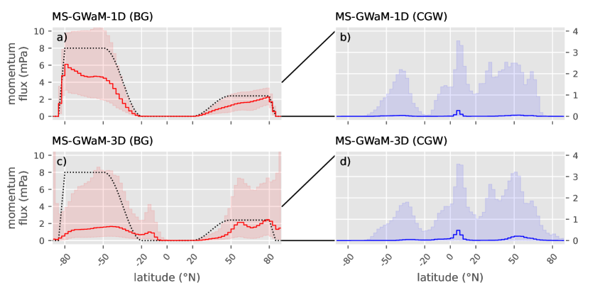
Figure 1: Zonally averaged absolute vertical fluxes of horizontal momentum at $16\,\mathrm{}{km}$ height for MS-GWaM-1D (a-b) and MS-GWaM-3D (c-d) for June 1991. The solid lines represent the 50th percentile (median), the surfaces show the ranges from the 10th to the 90th percentiles. Results are separated into background waves (a,c) and convectively generated waves (b,d). The black dotted lines represent the launched absolute momentum fluxes at $300\,\mathrm{}{hPa}$ during the summer solstice.

Similar to Bölöni et al. (2021) and Kim et al. (2021), the present implementation of MS-GWaM utilizes two sources of gravity waves as a lower boundary condition (Fig. 1). In particular, a background source in the middle to high latitudes, accounting, e.g. for IGWs emitted from jets and fronts, as well as a convective source, are employed. The former prescribes at a given launch level a seasonally varying pseudo-momentum flux with a spectral shape following the Desaubie spectrum (c.f. Orr et al., 2010). At the solstice, it has a latitudinal profile with winter hemispheric fluxes of $F_{w}=8\,\mathrm{}{mPa}$, no fluxes for latitudes $\phi\in$[$20^{\circ}$S, $20^{\circ}$N], and summer hemispheric fluxes of $F_{s}=2.4\,\mathrm{}{mPa}$. No background waves are launched at latitudes higher than $|\phi|>85^{\circ}$. The different regimes are connected through smooth transitions. The profile oscillates in time with a sinusoidal yearly cycle. Summarizing, we employ a latitudinal profile, $\alpha(\varphi)$, and a total absolute momentum flux at the lower boundary during the Northern summer solstice, $F_{sol}$,

$$\alpha(\varphi) =\begin{cases}\min\left(1,\max\left(0,1-\frac{\varphi-80}{5}\right)\right)&\mbox{if }\varphi\geq 80\\ 1,&\mbox{if }\varphi\in[50,80)\\ \frac{1}{2}\left(1-\cos\left(\pi\frac{\varphi-20}{30}\right)\right)&\mbox{if }\varphi\in[20,50)\\ 0&\mbox{else}\end{cases},$$ (22)

$$F_{sol}(\varphi) =\alpha(\varphi)F_{s}+\alpha(-\varphi)F_{w},$$ (23)

where $\varphi$ is the latitude in units ^∘N. The absolute momentum flux at the lower boundary condition then reads

$$F_{am} =\frac{1}{2}\left[\vphantom{\frac{1}{2}}F_{sol}(\varphi)(1+\cos\tau)\right.$$

$$\qquad+\left.F_{sol}(-\varphi)(1-\cos\tau)\vphantom{\frac{1}{2}}\right],$$ (24)

with the non-dimensional time difference, $\tau=2\pi(t-t_{sol})/1\,\mathrm{}{y}$, relative to the time of the Northern summer solstice, $t_{sol}$. These background waves are launched at a height corresponding to a pressure of $300\,\mathrm{}{hPa}$ (black, dotted line in Fig. 1a and c) with a momentum flux which is equally divided into 4 horizontal directions as done by Bölöni et al. (2021). This wave energy source is thus directionally homogeneous with a purely latitudinal profile on the $300\,\mathrm{}{hPa}$ pressure surface. Additionally, convectively generated waves are considered as described by Kim et al. (2021) with the same chosen parameters except for an increased area fraction of $\varepsilon_{q}=7\,\mathrm{}{\%}$, resulting in a reduced gravity wave flux. As an example of the resulting lower boundary conditions we show the absolute vertical momentum fluxes, defined by

$$F_{am}=\bar{\rho}\left(\left\langle w^{\prime}u^{\prime}\right\rangle^{2}+\left\langle w^{\prime}v^{\prime}\right\rangle^{2}\right)^{\frac{1}{2}},$$ (25)

through the surface at a constant height of $16\,\mathrm{}{km}$ for June 1991 (Fig. 1). The thick line presents the median of the zonally averaged fluxes during the month, and the shading around the median shows the range between the 10th and 90th percentiles highlighting the variability in the fluxes. Even though this height is rather close to the launch altitudes we observe that the horizontal wave propagation changes the statistics of the vertical fluxes of background waves (Fig. 1a and c). In contrast, the convectively generated waves show rather similar statistics at this altitude between MS-GWaM-3D and 1D (Fig. 1b and d).

The two sources of wave energy are accompanied by a saturation parametrization following Bölöni et al. (2016, 2021) which is based on the idea of Lindzen (1981) but in a spectrally integrated manner. In particular, the threshold for static instability is formulated for the wave action as follows,

$$\int\limits_{\mathbb{R}^{3}}\frac{k_{r}^{2}|\bm{k}_{h}|^{2}}{\hat{\omega}K^{2}}\mathcal{N}d^{3}k=\mathcal{P}<\frac{\bar{\rho}}{2}.$$ (26)

Note that for a quasi-monochromatic wave, this relation reduces to the well-known threshold, $|B_{w}|^{2}<N^{4}/k_{r}^{2}$, with $B_{w}$ being the amplitude of IGW buoyancy. The concept of the integrated density perturbation, $\mathcal{P}$, is then used in a discrete sense and rewritten as the sum over all physically overlapping ray volumes, $j$, at the location, $\bm{r}_{b}$, such that

$$\mathcal{P}=\sum\limits_{j}\mathcal{P}_{j}=\sum\limits_{j}\frac{k_{rj}^{2}|\bm{k}_{hj}|^{2}}{\hat{\omega}_{j}K_{j}^{2}}\mathcal{A}_{j}\alpha_{j}.$$ (27)

with $\mathcal{A}_{j}=\mathcal{N}_{j}\Delta k_{\lambda}\Delta k_{\phi}\Delta k_{r}$, and $\alpha_{j}$ the spatial fraction that the $j$th ray volume takes of the volume of the cell that contains. Thus, rather than each individual spectral component, we consider a spectrally integrated saturation. The reduction of the individual wave action components, $\mathcal{A}_{j}$, to their saturation value, $\mathcal{A}_{j}^{*}$, is then achieved through setting

$$\mathcal{N}_{j}\rightarrow\mathcal{N}_{j}^{*}=\mathcal{N}_{j}\left[1-2\kappa K_{j}^{2}\Delta t\right],$$ (28)

with the turbulent diffusivity coefficient

$$\kappa=\max\left(0,\frac{\mathcal{P}-\frac{\bar{\rho}}{2}}{2\Delta t\sum\limits_{j}\mathcal{P}_{j}K_{j}^{2}}\right).$$ (29)

Saturation is thus triggered where the instability threshold (Eq. 26) is violated by the constructive interference of locally overlapping internal waves. All wave amplitudes, or equivalently wave action densities, are then set to the corresponding saturation values. Note that Eq. (29) does not imply that the turbulent diffusivity diverges as $\Delta t\rightarrow\infty$. Because at the beginning of each time step $\mathcal{P}\leq\frac{\bar{\rho}}{2}$, the numerator of the ratio is at best growing linearly with $\Delta t$ so that $\kappa$ always ends up finite.

4 Atmospheric simulations with UA-ICON and MS-GWaM-3D

Building on Bölöni et al. (2021) and Kim et al. (2021), who introduced MS-GWaM-1D, we choose to work with the ICON model with its upper-atmosphere extension (Zängl et al., 2015; Borchert et al., 2019). Here, we use version 2.6.2-nwp4 with a horizontal resolution of approximately $160\,\mathrm{}{km}$ (model grid R2B04) and the physics packages for the numerical weather prediction (NWP) and the upper atmosphere. The setup has a model top of $150\,\mathrm{}{km}$ with vertical grid extent of a few tens of meters in the boundary layer, $700-1500\,\mathrm{}{m}$ in the stratosphere, and a maximum of approximately $4\,\mathrm{}{km}$ in the lower thermosphere. A sponge layer acts above an altitude of $110\,\mathrm{}{km}$ which is why we restrict our analysis to altitudes below $100\,\mathrm{}{km}$. The model is initialized with IFS analysis data below $60\,\mathrm{}{km}$ and with the climatological thermodynamic state at rest above. It is then spun up for a month to exclude adjustment effects in our analysis. These runs are repeated to simulate June and December for the years 1991 through 1998. Additionally, we deploy runs for June and December 1991 with extended diagnostics. In particular, the free parameters controlling the launch fluxes are the convective area fraction for the convectively generated waves and the summer and winter launch amplitudes of the background waves (see Sec. 33.3). In general, stronger gravity-wave launch fluxes shift the wave saturation to lower altitudes leading to a lower wind reversal at the mesopause. Comparisons of simulations with the horizontal wind model HWM (hereafter HWM2014, Drob et al., 2015) and the empirical temperature model NRLMSIS2.1 (hereafter MSIS, Emmert et al., 2022) then give a good estimate for the performance of the chosen parameters. With the help of short simulations spanning a large parameter space, we identified an optimum with an area fraction of $\varepsilon_{q}=7\,\mathrm{}{\%}$, a winter launch flux of $F_{w}=8\,\mathrm{}{mPa}$, and a summer launch flux of $F_{s}=2.4\,\mathrm{}{mPa}$ (for more detail see Sec. 33.3).

4.1 Zonal mean flow

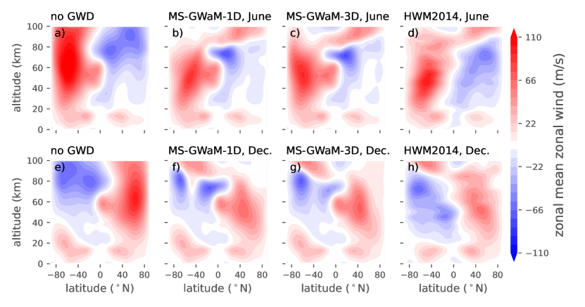
Figure 2: Zonal mean zonal winds from composites of runs for June (a-d) and December (e-h). The composites correspond to averages for the years 1991 through 1998. Runs from MS-GWaM-1D (b, f) and MS-GWaM-3D (c, g) are compared to simulations without any non-orographic IGW parameterization (a, e) and the HWM2014 climatologic model (d, h).

To test the general performance of the gravity wave parametrization we analyze the zonal-mean zonal wind and temperatures as composites over 8 simulations of June and December (Fig. 2 and 3). To highlight the general effect of the parametrizations and visualize the general model performance, we accompany the data from simulations without non-orographic gravity wave parameterization. Naturally, the runs including a gravity wave drag parametrization mend model biases and thus differ significantly from the runs without. The comparison is, therefore, to be understood as a reference for the general behavior of ICON in the present setup and in how far model biases stem from the lack of a gravity wave drag parametrization or may be rooted elsewhere. Additionally, we show the reference climatologies HWM2014 and MSIS. Note that, as described above, both versions of MS-GWaM were tuned such that the mesopause height at $z\approx 80$km agrees with the HWM2014. In general, MS-GWaM-1D and 3D produce physical zonal-mean zonal winds with the expected wind reversals in both the summer and winter hemispheres (Fig. 2b-d, f-h). As one may expect, runs with the same model setup but without any non-orographic parameterization are subject to very strong jets and entirely lack the mesopause reversal (Fig. 2a and e).

Notable differences to the HWM2014 can be seen in the summer hemispheric jets, in the tropical stratosphere, and in the Antarctic winter jet. Comparing the two MS-GWaM results with the run without any non-orographic gravity wave drag parameterization (Fig. 2a and e) we find that both the weak summer hemispheric jet and the tropical stratospheric jet at $z\approx 50$km height are robust features of the current model version, which are present in all three runs. The aforementioned tuning runs covering the parameter space of the parametrization also indicated that there is little to no influence on both structures (not shown). We thus conclude that these are generally independent of the used gravity wave parameterization. Moreover, we observe that the slant of the Antarctic winter jet towards the equator is not entirely reproduced by MS-GWaM-3D (Fig. 2c). This is due to a weaker gravity wave drag near the south pole above $60\,\mathrm{}{km}$ altitude in MS-GWaM-3D as opposed to MS-GWaM-1D. Possible reasons for that reduced wave drag might be improper spectral characteristics of the current background source, errors near the pole due to the representation of the ray-volume extent in spherical coordinate systems (c.f. 33.1), or even codependencies of the columnar gravity wave parameterization with other parameterizations such as the radiation scheme or the modified ozone climatology. In general, the confidence in the present implementation is high as MS-GWaM-1D was validated by Bölöni et al. (2021); Kim et al. (2021) and MS-GWaM-3D was validated against the results of Wei et al. (2019) using an idealized cubic geometry implemented in ICON (not shown). However, a more detailed analysis may be needed to identify the reasons behind the phenomenon and mend the setup accordingly.

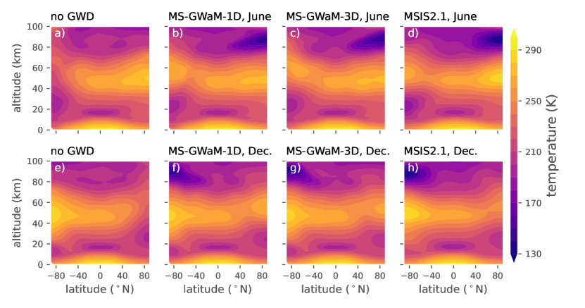
Figure 3: Like Fig. 2 but for zonally averaged temperatures. For comparison, we show the climatological model MSIS2.1 (d, h).

Similar to the zonally averaged zonal winds, we find that the zonally averaged temperatures and the corresponding MSIS fields agree well (Fig. 3). In particular, the MS-GWaM reproduces the cold summer pole at the mesopause as well as the warm winter pole associated with the stratopause (Fig. 3b-c and f-g). These features are naturally not present when the non-orographic gravity wave drag parameterization is switched off (Fig. 3a and e).

Except for the Antarctic winter jet, the zonal-mean model state generally seems to be affected only slightly by enabling a 3-dimensional wave propagation in MS-GWaM. This resembles the findings of Bölöni et al. (2021) where a weak dependency of the zonal-mean wind on the transience of the gravity wave parameterization was detected. Albeit somewhat counter-intuitive, it may not be a surprise as the spatial and temporal averages represent the quasi-steady state of the model setups. These in turn are tuned to approximate a similar zonal-mean model state. It was, however, also shown that both the transience as well as the localization of the gravity waves can have significant impacts on the structure of the horizontal mean flow (e.g. Sato et al., 2009; Sacha et al., 2016; Ehard et al., 2017). For instance, the mean-state results may change if a more realistic spatio-temporal distribution of the wave source spectrum was employed. While the investigation of realistic source distribution is left for future work, in the following sections we focus on the nature of 3-dimensional propagation of parameterized IGWs, examining wave action fluxes and budgets as well as horizontal structures of IGW momentum fluxes and zonal mean wave drags.

4.2 Global 3-dimensional IGW distribution

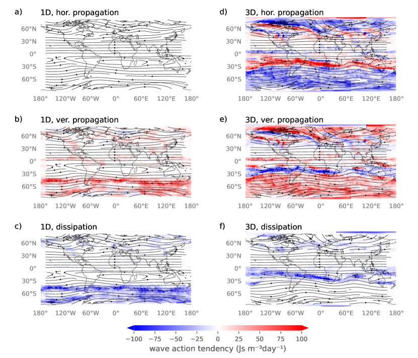
Figure 4: Wave action tendencies for MS-GWaM-1D (a-c) and MS-GWaM-3D (d-f) due to horizontal wave propagation (a, d), vertical wave propagation (b, e) and wave dissipation (c, f). All tendencies are 10-day averages for June 10-20 1991 at an altitude of $z\approx 25.1\,\mathrm{}{km}$. Additionally, streamlines of the horizontal wind are shown.

Gravity waves are generally 3-dimensional phenomena that are present in large parts of the atmosphere. While wave-resolving simulations can give insights into global wave activity, they typically span short model times due to the limitations of both computational resources as well as the required storage. Additionally, the separation of IGWs from other dynamics and their characterization are generally non-trivial tasks. Being based on a multiscale WKBJ theory (Achatz et al., 2017), MS-GWaM simulates the global behavior of non-orographic gravity waves without the need to explicitly resolve their fast varying phases. As a result, it can be used to predict global distributions of phase-space wave action densities as well as derived quantities such as momentum fluxes and the resulting wave drag. As an example, we analyze the global wave action budget as follows.
Consider the phase-space integrated wave action conservation (Eq. 8), averaged in time,

$$-\frac{\Delta\mathcal{A}}{\Delta t} =\nabla_{h}\cdot\overline{\bm{c}_{gh}\mathcal{A}}+\partial_{r}\overline{c_{gr}\mathcal{A}}+\overline{S},$$ (30)

where we define $(\bm{c}_{gh},c_{gr})\mathcal{A}=\int(\bm{c}_{gh},c_{gr})\mathcal{N}d^{3}k$, and the overbars denote the temporal average over the time interval, $\Delta t$. Here, the three right-hand side terms correspond to the temporally averaged wave-action tendency contributions from the horizontal wave propagation, the vertical wave propagation, and the wave saturation. Moreover, the left-hand term is small for sufficiently long averaging intervals. For a sufficiently small left-hand-side of Eq. (30) while preserving the planetary wave structure, we choose $\Delta t=10\,\mathrm{}{d}$ and show the predictions of the right-hand side contributions by MS-GWaM-1D and -3D at an altitude of $z\approx 25.1\,\mathrm{}{km}$ for June 10-20, 1991. As one may expect, MS-GWaM-1D predicts a balance between the vertical propagation and the wave dissipation (Fig. 4b and c). Thus, wave breaking and strong mean-flow generation can only occur where IGWs were previously able to vertically propagate through the wind shear of the underlying air column. At the rather low altitude of $25\,\mathrm{}{km}$ this results in a rather uniform distribution being strongest in the winter (i.e. Southern) hemisphere (Fig. 4c). Running the same case with MS-GWaM-3D we find that both the contributions due to the horizontal and vertical propagation are of similar magnitude such that the resulting balance includes all terms (Fig. 4d through f). Near horizontally sheared wind structures, such as the edges of the Antarctic winter jet, the two contributions from the horizontal and vertical propagation form inverted dipoles associated with wave refraction phenomena. In the case of the mentioned Antarctic winter jet, as we will show below, this corresponds to the often observed wave refraction into the jet (e.g.  Ehard et al., 2017; Hindley et al., 2020; Gupta et al., 2021). Interestingly, the wave refraction follows the structure of the resolved planetary waves and ultimately leads to a shift of lower-level wave dissipation towards regions of strong horizontal shear as for instance found between the summer and winter jets (Fig. 4f). Despite the different launch amplitudes (see Sec. 33.3) all contributions have similar magnitudes on both hemispheres.

4.3 Wave propagation in the vicinity of horizontally sheared jet structures

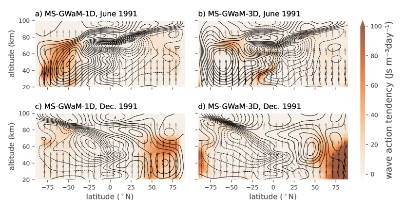
Figure 5: Wave action changes due to wave propagation in MS-GWaM-1D (a,c) and MS-GWaM-3D (b,d) for June 1991 (a-b) and December 1991 (c-d). The field is overlaid with vectors of wave action fluxes. They are scaled with respect to the plot dimensions and units, the horizontal direction is enhanced by a factor of 3 for visualization. The arrow transparency represents the wave action flux strength. The contours represent the corresponding zonally-averaged zonal wind with $10\,\mathrm{}{ms^{-1}}$ increments, with dashed and solid lines for negatives and non-negatives, respectively.

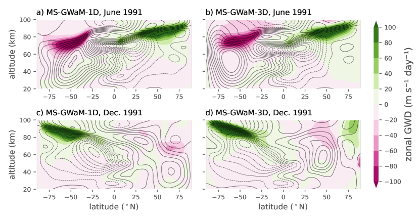
Figure 6: Zonnally-averaged zonal gravity wave drag due to the parametrized, non-orographic internal gravity waves. The results are averaged over June 1991 (a-b) and December 1991 (c-d) and plotted for both MS-GWaM-1D (a,c) and MS-GWaM-3D (b,d). The contours represent the corresponding zonally-averaged zonal wind with $10\,\mathrm{}{ms^{-1}}$ increments.

Expanding on the horizontal refraction behavior found in the horizontal maps (Fig. 4) we show zonal averages of wave action fluxes (Fig. 5) and the corresponding wave drag (Fig. 6) temporally averaged over free runs for June 1991 (both figures panels a and b) and December 1991 (both figures panels c and d). By construction, MS-GWaM-1D only allows for vertical propagation (Fig. 5a and c). The corresponding wave-action tendency is thus associated with the vertical wave-action flux convergence. The consequently generated wave drag accelerates the zonal wind structures with maxima occurring at the mesopause (Fig. 6a and c). In contrast, MS-GWaM-3D shows strong horizontal propagation in regions of strong horizontal and vertical shear such as jet edges (Fig. 5b and d). Notably, in southern-hemispheric winter the wave action flux vector points northward near the South Pole, i.e. into the Southern winter jet, (Fig. 5b). Consequently, the polar wave-action fluxes are reduced at altitudes near the mesopause and the wave drag maximum shifts northward (Fig. 5b and Fig. 6b). Moreover, the Southern winter jet is somewhat too strong at higher altitudes and high latitudes. This effect might be an important reason for the corresponding discrepancies observed in the zonal-mean zonal wind (c.f. Sec. 44.1 and Fig. 2c). Although we cannot exclude other sources of the bias, the shifted wave drag due to 3D propagation suggests some underlying physics that is possibly not well understood (such as secondary wave generation) or compensated by the tuning of other physics parameterizations in classical 1D setups (such as the radiation scheme). Further and more targeted investigation may be needed to bring clarity about this effect.

Similar refraction behavior can also be seen in the summer hemispheres. However, the model biases of the Northern summer hemispheric jet structures (c.f. Sec. 44.1) complicate the interpretation of the wave action budgets in the corresponding regions.

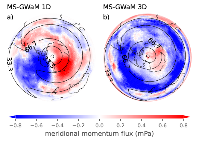
Figure 7: Meridional momentum fluxes in MS-GWaM-1D (a) and MS-GWaM-3D (b) for composites of Junes from 1991 through 1998 at an altitude of $z\approx 39.8\,\mathrm{}{km}$ overlaid by the corresponding zonal winds (contours, units in $\,\mathrm{}{ms^{-1}}$). The maps show the typically observed refraction of internal gravity waves into the Southern polar night jet and modified wind patterns.

To further highlight the effect of the 3-dimensional transient wave refraction behavior around the polar winter jet we show the meridional momentum fluxes from the composites of June for the years 1991 through 1998 (Fig. 7). Note that the meridional fluxes of MS-GWaM-1D must be interpreted keeping in mind the assumed local horizontal homogeneity. That is, albeit the wave parameters suggest horizontal momentum fluxes, the horizontal propagation (including the wave advection) are set to zero in the columnar setup. The resulting synthetic meridional fluxes seem to be unrelated to the underlying jet structure (Fig. 7a). As waves are launched homogeneously in all directions at the lower boundary (Sec. 33.3) the resulting meridional fluxes are a product of the partial wave filtering due to local vertical gradients of both the horizontal wind and the buoyancy frequency. In contrast, MS-GWaM-3D shows meridional convergence of wave momentum fluxes into the polar jet (Fig. 7b). This feature is robust throughout all simulations and compares well to both satellite and ground-based observations (e.g.  Ehard et al., 2017; Hindley et al., 2020; Gupta et al., 2021). As discussed above, the resulting wave dissipation maximum is shifted northward as compared to the columnar approach of MS-GWaM-1D. It thus leads to a shifted wave drag which in turn influences the zonal-mean jet structure.

5 Discussion of achievements and challenges

Although internal gravity waves (IGWs) are an essential part of atmospheric dynamics, their parameterization in general circulation models is typically subject to various simplifications. In particular, the single-column assumption, the steady-state approximation, and the balanced mean-flow assumption have usually been made. Here, we present a fully 3-dimensional implementation of the Multi-Scale Gravity Wave Model, MS-GWaM-3D, which aims at parameterizing IGWs through Lagrangian ray-tracing without the three mentioned assumptions. In general, we find that including 3D transience significantly impacts global IGW propagation patterns and thus horizontal IGW distributions. Correspondingly, the associated wave drag and mean flows are modified.

We compare two distinct situations: For MS-GWaM-1D, where the columnar approximation is applied, the vertical propagation is balanced by wave breaking in the wave action equation (Fig. 4b and c). Only waves that did not encounter critical layers according to their wave properties may propagate to higher altitudes and eventually break. In contrast, MS-GWaM-3D allows for modulated and spatially unconstrained propagation and enables waves to be refracted around wind structures. As a consequence, both the horizontal and vertical propagation balance with the wave dissipation (Fig. 4). The equal order of magnitude in the contributions of the horizontal and vertical wave propagation to the wave action budget emphasizes the importance of including horizontal propagation. Moreover, it questions the validity of using columnar methods when, e.g., studying IGW distributions. Both methods do, however, perform as expected in reproducing the cold summer pole and the warm winter pole at altitudes $\sim 85\,\mathrm{}{km}$ and $\sim 60\,\mathrm{}{km}$, respectively, in the climatological zonal mean (Fig. 3). The corresponding wind reversals and the mesopause altitudes are reasonably predicted (Fig. 2). We are thus confident that MS-GWaM-3D, as MS-GWaM-1D before it, covers some major effects of IGWs on the mean-flow dynamics, rendering MS-GWaM-3D a viable IGW parameterization. The 3D wave propagation is also found to have significant impacts on the variability of the zonal-mean flow, such as the quasi-biennial oscillation (QBO), which will be presented in a separate paper.

Including the horizontal propagation does, however, also introduce some important differences in the simulated climatology. In particular, the southern hemispheric winter jet becomes stronger near the pole at altitudes $\sim 60-80\,\mathrm{}{km}$ for MS-GWaM-3D (Fig. 2c). The reason behind this change is, however, not obvious. One possible explanation is the northward refraction of wave action near the Antarctic winter jet in MS-GWaM-3D as compared to MS-GWaM-1D. Both the 3D wave action tendencies (dipole structures in Fig. 4d and e) and the zonally averaged wave action fluxes (vectors in Fig. 5a and b) suggest that the 3D modulation causes IGWs to propagate northward and thus relate to a weaker gravity wave drag at high altitudes and similar latitudes (Fig. 6a and b). Additionally, the meridional momentum fluxes around the Antarctic winter jet support this finding (Fig. 7). We have high confidence in these patterns as they are backed by a multitude of observations and wave-resolving model studies (e.g. Ehard et al., 2017; Hindley et al., 2020; Gupta et al., 2021). The refraction of waves into the jet may consequently result in the too-strong zonal-mean zonal wind further south and at higher altitudes. It remains unclear, however, whether there are more factors influencing the result. Possible other candidates are the simplifications made in the setup of the numerical ray-tracer in the spherical coordinate system or codependencies of the gravity wave parameterization with other parameterizations, for example, the ozone climatology and the radiation scheme. A thorough investigation will be needed and we hope to answer these questions in an envisioned follow-up study. Finally, the simulations presented here also reveal some limitations of the general model setup. In particular, we observe weak winds in the summer stratosphere independent of the gravity wave parameterization.

There is a long list of effects that may be analyzed in more detail from this starting point. Notably, the role of IGWs in sudden stratospheric warmings, the accuracy of the final warming date, the missing wave drag at $60^{\circ}$S, etc. are of interest and are planned for future simulations and analyses. Current investigations include the impact of 3D-transient waves on the quasi-biennial oscillation and wave intermittency. Moreover, there are efforts into increasing the realism of the included IGW sources related to jets-frontal systems and flow over topography. Finally, code optimization may reduce the computational cost which amounts to a runtime factor $\sim 30$ with respect to runs without any non-orographic wave drag parameterization (c.f. Appendix E). With these challenges in mind, we ultimately aim for the application of MS-GWaM-3D in climate simulations and possibly numerical weather predictions.

Furthermore, there are numerous potential improvements that may be added to MS-GWaM in the future albeit not considered here. Most importantly, MS-GWaM-3D—for the time being—does not include a flow-dependent description of the emission of GWs from jets and fronts (Charron and Manzini, 2002; Richter et al., 2010; Cámara and Lott, 2015) or flow over topography (Palmer et al., 1986; Bacmeister et al., 1994; Lott and Miller, 1997; van Niekerk and Vosper, 2021; van Niekerk et al., 2023). For the latter reason, MS-GWaM needs augmentation with a subgrid-scale orography parameterization. Moreover, it is not clear how important modulated triadic resonant interactions among IGWs or between subgrid-scale geostrophic modes and IGWs are for atmospheric dynamics, which could, however, be investigated through raytracing techniques (c.f. Kafiabad et al., 2019; Voelker et al., 2020).

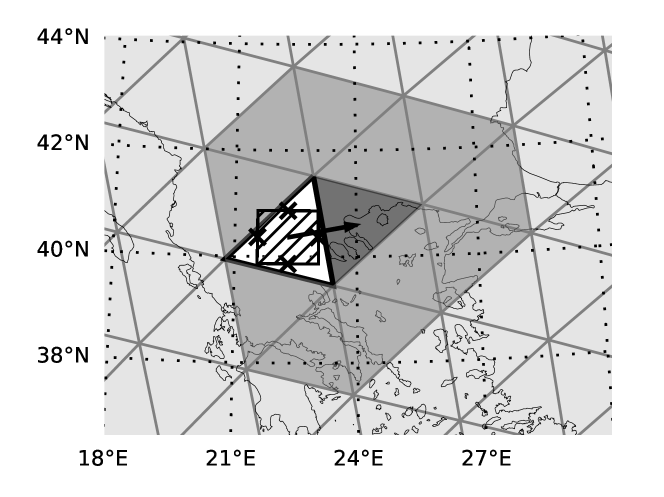
Figure 8: Sketch of the horizontal extent of a Lagrangian ray volume propagating in the unstructured triangular grid of the ICON model. The propagating ray volume (hatched box) may be associated with a current parent column (framed white grid cell). Given a horizontal group velocity (black arrow) we may expect it to propagate into a neighboring column (dark gray shaded grid cell). The crosses at the edges of the ray volume mark the locations for which background field data is needed to calculate the propagation of the ray volume.

Appendix A 3-dimensional field interpolation

When calculating the propagation of a finite-size ray volume in an inhomogeneous medium it is important to consider that even under the assumption that all wave numbers are constant throughout the volume the group velocities can differ significantly within the same ray volume. In particular, the scale height correction, $\Gamma$, the Brunt-Väisälä frequency, $N$, and the mean winds, $\bm{U}$, are functions of space and differ between the four faces forming with the meridional and zonal boundaries of the ray volume (see crosses in Fig. 8). To account for a corresponding change in the area of the ray volume we interpolate all needed background fields horizontally to the face-center positions and the ray volume center through linear Taylor expansions as follows:

$$\chi(\bm{r}_{\mbox{\scriptsize j}})=\chi(\bm{r}_{\mbox{\scriptsize cc}})+\left[\nabla_{\bm{r}}\chi\right]_{\mbox{\scriptsize cc}}\cdot(\bm{r}_{\mbox{\scriptsize j}}-\bm{r}_{\mbox{\scriptsize cc}}),$$ (31)

where $\chi$ symbolizes the interpolated field and the subscripts cc and j refer to evaluations at the cell center and the ray-volume face or ray-volume center, respectively. In the vertical, we apply linear interpolations between the grid points. While the tendencies for the wave numbers are computed with the ray-volume centered values, the interpolated fields at the ray volume faces are used to compute group velocities enabling the prediction of the changing extent of the ray volume in physical space (Eqs. 2.1 to 2). In particular, the difference in the group velocities at the center of opposing ray-volume faces predicts the rate of compression along the corresponding direction. The average of the opposing group velocities is then used to predict the change of location along the characteristic (Eq. 3). Consequently, the change in the wave number extents $\Delta(k_{\lambda},k_{\phi},k_{r})$ are determined following the procedure described in section 33.1.

Appendix B Horizontal propagation and code parallelization

Since MS-GWaM propagates Lagrangian ray volumes through space, it cannot easily be parallelized using the traditional MPI infrastructure of the ICON model developed for the synchronization of Eulerian fields. In particular, the ray volumes may propagate over large distances and transfer between parallel MPI domains. To accompany this while avoiding load balancing problems we associate each ray volume with a parent cell based on its current location and store it in a corresponding grid-based array. As an example, in the shown sketch (Fig. 8) the hatched ray volume is associated with the white-bounded underlying cell. It may, however, have a group velocity such that it propagates into a new parent cell, represented by the arrow and the dark gray shaded triangle, respectively. Therefore after each propagation step all cells such as the dark gray shaded triangle search all rays in all neighboring cells (light gray shading) and transfer those that are now located in their own cell area. With this construction, we can localize arrays of ray volumes based on the Eulerian grid column. The integration along the wave characteristics, launch processes, saturation calculations, and wave projection onto the Eulerian grid can then be parallelized using the domain decomposition of the dynamical core with the given model infrastructure. Note that the modulation equations are integrated using a 3-step Runge-Kutta low-storage scheme (Williamson, 1980).

Appendix C Ray volume splitting

In general the numerical treatment of internal gravity waves as ray volumes are set up to be exact in the limit of infinitesimally small ray volumes and Eulerian grid cells. The actual sizes of both are, however, finite. While the total phase-space volume of the rays is constant by construction, they may stretch or compress either in physical or spectral space. To avoid large numerical artifacts we therefore split all ray volumes, $j$, vertically which become larger than the local thresholds

$$\Delta r_{j}>\max(\alpha_{s}h_{c},1\,\mathrm{}{km}),$$ (32)

with the local grid-cell height, $h_{c}$, and a scale factor $\alpha_{s}$ (which is set to 2.5 in this study). The volume is cut into two equally sized ray volumes in the vertical with the wave vectors identical to the original parent wave. The carrier ray location of each split volume is then set to its center. Similarly, ray volumes are split horizontally where either of the three thresholds is reached

$$\cos\phi_{j}\Delta\lambda_{j} >\alpha_{s}\sqrt{a_{c}}/R,$$

$$\Delta\phi_{j} >\alpha_{s}\sqrt{a_{c}}/R,$$ (33)

$$\cos\phi_{j}\Delta\lambda_{j}\Delta\phi_{j} >\alpha_{s}a_{c}/R^{2}.$$

Here, $a_{c}$ represents the local cell area, and $R$ the Earth mean radius. Splitting is done along the direction of the larger extent.

Appendix D Horizontal flux smoothing

To avoid numerical artifacts based on the employed simplification in the ray volume representation we smooth all diagnostic outputs and wave fluxes. Each triangular cell combines three vertices, one in each corner (c.f. Fig. 8). Each of these vertices is connected to five or six neighboring cells, depending on the location of the triangulated icosahedron. The smoothing algorithm first averages the corresponding fields over these pentagons or hexagons and then combines the three resulting values into one average. Consequently, the weights are distributed such that the center cell is weighted with a factor $3$, the direct adjacent cells with one common edge are weighted with a factor $2$, and all neighboring cells sharing a vertex with the center cell are weighted with a factor $1$. While this procedure generally reduces the amplitude of strong flux peaks it also reduces the occurrence of grid-scale noise and ensures model stability.

Appendix E Computational performance

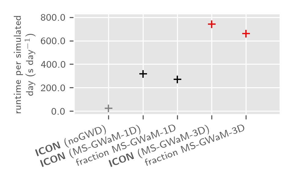
Figure 9: Performance comparison for UA-ICON at the R2B4 resolution ($\sim 160$km) parallelized over 1920 MPI cores for runs without IGW parameterization (gray), MS-GWaM-1D (black) and MS-GWaM-3D (red). In addition to the total run time of ICON per simulated day we show the fraction of run time associated with MS-GWaM-1D and -3D. The median values for the three setups are $25\,\mathrm{}{s/day}$, $317\,\mathrm{}{s/day}$, and $743\,\mathrm{}{s/day}$ and thus MS-GWaM-1D and-3D slow down the model by about a factor of 12 and 30, respectively.

Finally, conceptional models need to prove themselves not only through the accurate representation of not-resolved physics but also through competitive performance. In particular, ray-tracing models may suffer from load balancing problems due to the uneven distribution of ray integrations between processors but also the existence of too many rays in general. As described in Sec. B, MS-GWaM utilizes a cell-based representation of ray volumes which is highly parallelizable such that load balancing problems may not inhibit the model performance. Additionally, the total number of ray volumes is restricted by the maximum numbers $n_{bg}\leq 4800$ and $n_{conv}\leq 8800$ per model-grid column for background and convective gravity waves, respectively. For the lowest impact, the ray volumes with the lowest wave energy are chosen to be removed. Detailed analyses show that the impact of this procedure is indeed small and may be neglected (not shown).

To measure the performance of the model we compare the runtimes of all two-month runs without any non-orographic gravity wave parameterization with both the MS-GWaM-1D and MS-GWaM-3D setups (Fig. 9). Additionally, we show the fraction of runtime that is associated with MS-GWaM and normalize all values with the number of simulated days. These measures show that MS-GWaM-1D and MS-GWaM-3D slow down ICON by factors approximately 12 and 30, respectively. That is, the 3D setup has performance penalty equal to a factor of approximately 2.5 Still, the gravity wave parameterization is several orders of magnitude faster than wave-resolving simulations - for which Bölöni et al. (2021) estimate a cost factor of about six orders of magnitude - and thus a competitive tool for the estimate and analysis of global IGW effects.

References

- Achatz (2022) Achatz, U., 2022: Atmospheric Dynamics. 1st ed., Springer Berlin Heidelberg, URL https://link.springer.com/book/9783662639429.
- Achatz et al. (2017) Achatz, U., B. Ribstein, F. Senf, and R. Klein, 2017: The interaction between synoptic-scale balanced flow and a finite-amplitude mesoscale wave field throughout all atmospheric layers: weak and moderately strong stratification. Quarterly Journal of the Royal Meteorological Society, 143 (702), 342–361, 10.1002/qj.2926.
- Alexander and Dunkerton (1999) Alexander, M. J., and T. J. Dunkerton, 1999: A Spectral Parameterization of Mean-Flow Forcing due to Breaking Gravity Waves. Journal of the Atmospheric Sciences, 56 (24), 4167–4182, 10.1175/1520-0469(1999)056¡4167:ASPOMF¿2.0.CO;2, URL https://journals.ametsoc.org/view/journals/atsc/56/24/1520-0469˙1999˙056˙4167˙aspomf˙2.0.co˙2.xml, publisher: American Meteorological Society Section: Journal of the Atmospheric Sciences.
- Alexander et al. (2010) Alexander, M. J., and Coauthors, 2010: Recent developments in gravity-wave effects in climate models and the global distribution of gravity-wave momentum flux from observations and models. Quarterly Journal of the Royal Meteorological Society, 136 (650), 1103–1124, 10.1002/qj.637, URL https://onlinelibrary.wiley.com/doi/abs/10.1002/qj.637, _eprint: https://onlinelibrary.wiley.com/doi/pdf/10.1002/qj.637.
- Amemiya and Sato (2016) Amemiya, A., and K. Sato, 2016: A New Gravity Wave Parameterization Including Three-Dimensional Propagation. Journal of the Meteorological Society of Japan. Ser. II, 94 (3), 237–256, 10.2151/jmsj.2016-013.
- Bacmeister et al. (1994) Bacmeister, J. T., P. A. Newman, B. L. Gary, and K. R. Chan, 1994: An Algorithm for Forecasting Mountain Wave–Related Turbulence in the Stratosphere. Weather and Forecasting, 9 (2), 241–253, 10.1175/1520-0434(1994)009¡0241:AAFFMW¿2.0.CO;2, URL https://journals.ametsoc.org/view/journals/wefo/9/2/1520-0434˙1994˙009˙0241˙aaffmw˙2˙0˙co˙2.xml, publisher: American Meteorological Society Section: Weather and Forecasting.
- Borchert et al. (2019) Borchert, S., G. Zhou, M. Baldauf, H. Schmidt, G. Zängl, and D. Reinert, 2019: The upper-atmosphere extension of the ICON general circulation model (version: Ua-icon-1.0). Geoscientific Model Development, 12 (8), 3541–3569, 10.5194/gmd-12-3541-2019, URL https://doi.org/10.5194/gmd-12-3541-2019.
- Bretherton (1966) Bretherton, F. P., 1966: The propagation of groups of internal gravity waves in a shear flow. Quarterly Journal of the Royal Meteorological Society, 92 (394), 466–480, 10.1002/qj.49709239403, URL http://doi.wiley.com/10.1002/qj.49709239403, publisher: John Wiley & Sons, Ltd.
- Bölöni et al. (2021) Bölöni, G., Y.-H. Kim, S. Borchert, and U. Achatz, 2021: Toward Transient Subgrid-Scale Gravity Wave Representation in Atmospheric Models. Part I: Propagation Model Including Nondissipative Wave–Mean-Flow Interactions. Journal of the Atmospheric Sciences, 78 (4), 1317–1338, 10.1175/JAS-D-20-0065.1, URL https://journals.ametsoc.org/view/journals/atsc/78/4/JAS-D-20-0065.1.xml, publisher: American Meteorological Society Section: Journal of the Atmospheric Sciences.
- Bölöni et al. (2016) Bölöni, G., B. Ribstein, J. Muraschko, C. Sgoff, J. Wei, and U. Achatz, 2016: The Interaction between Atmospheric Gravity Waves and Large-Scale Flows: An Efficient Description beyond the Nonacceleration Paradigm. Journal of the Atmospheric Sciences, 73 (12), 4833–4852, 10.1175/JAS-D-16-0069.1, URL http://journals.ametsoc.org/doi/10.1175/JAS-D-16-0069.1.
- Charron and Manzini (2002) Charron, M., and E. Manzini, 2002: Gravity Waves from Fronts: Parameterization and Middle Atmosphere Response in a General Circulation Model. Journal of the Atmospheric Sciences, 59 (5), 923–941, 10.1175/1520-0469(2002)059¡0923:GWFFPA¿2.0.CO;2, URL https://journals.ametsoc.org/view/journals/atsc/59/5/1520-0469˙2002˙059˙0923˙gwffpa˙2.0.co˙2.xml, publisher: American Meteorological Society Section: Journal of the Atmospheric Sciences.
- Cámara and Lott (2015) Cámara, A. d. l., and F. Lott, 2015: A parameterization of gravity waves emitted by fronts and jets. Geophysical Research Letters, 42 (6), 2071–2078, 10.1002/2015GL063298, URL https://onlinelibrary.wiley.com/doi/abs/10.1002/2015GL063298, _eprint: https://onlinelibrary.wiley.com/doi/pdf/10.1002/2015GL063298.
- Drob et al. (2015) Drob, D. P., and Coauthors, 2015: An update to the Horizontal Wind Model (HWM): The quiet time thermosphere. Earth and Space Science, 2 (7), 301–319, 10.1002/2014EA000089, URL https://agupubs.onlinelibrary.wiley.com/doi/10.1002/2014EA000089.
- Ehard et al. (2017) Ehard, B., and Coauthors, 2017: Horizontal propagation of large-amplitude mountain waves into the polar night jet. Journal of Geophysical Research: Atmospheres, 122 (3), 1423–1436, 10.1002/2016JD025621, URL https://onlinelibrary.wiley.com/doi/abs/10.1002/2016JD025621, _eprint: https://onlinelibrary.wiley.com/doi/pdf/10.1002/2016JD025621.
- Emmert et al. (2022) Emmert, J. T., and Coauthors, 2022: NRLMSIS 2.1: An Empirical Model of Nitric Oxide Incorporated Into MSIS. Journal of Geophysical Research: Space Physics, 127 (10), 10.1029/2022JA030896, publisher: John Wiley and Sons Inc.
- Fritts and Alexander (2003) Fritts, D. C., and M. J. Alexander, 2003: Gravity wave dynamics and effects in the middle atmosphere. Reviews of Geophysics, 41 (1), 1/1003, 10.1029/2001RG000106, URL http://doi.wiley.com/10.1029/2001RG000106, publisher: Wiley-Blackwell.
- Grimshaw (1974) Grimshaw, R., 1974: Internal gravity waves in a slowly varying, dissipative medium. Geophysical Fluid Dynamics, 6 (2), 131–148, 10.1080/03091927409365792, URL https://www.tandfonline.com/doi/abs/10.1080/03091927409365792, publisher: Informa UK Limited.
- Grimshaw (1975) Grimshaw, R., 1975: Nonlinear internal gravity waves in a rotating fluid. Journal of Fluid Mechanics, 71 (3), 497–512, 10.1017/S0022112075002704, publisher: Cambridge University Press.
- Gupta et al. (2021) Gupta, A., T. Birner, A. Dörnbrack, and I. Polichtchouk, 2021: Importance of Gravity Wave Forcing for Springtime Southern Polar Vortex Breakdown as Revealed by ERA5. Geophysical Research Letters, 48 (10), 10.1029/2021GL092762.
- Hasha et al. (2008) Hasha, A., O. Bühler, and J. Scinocca, 2008: Gravity Wave Refraction by Three-Dimensionally Varying Winds and the Global Transport of Angular Momentum. Journal of the Atmospheric Sciences, 65, 2892–2906, 10.1175/2007JAS2561.1.
- Hindley et al. (2020) Hindley, N. P., C. J. Wright, L. Hoffmann, T. Moffat-Griffin, and N. J. Mitchell, 2020: An 18-Year Climatology of Directional Stratospheric Gravity Wave Momentum Flux From 3-D Satellite Observations. Geophysical Research Letters, 47 (22), 10.1029/2020GL089557, publisher: Blackwell Publishing Ltd.
- Hines (1997a) Hines, C. O., 1997a: Doppler-spread parameterization of gravity-wave momentum deposition in the middle atmosphere. Part 1: Basic formulation. Journal of Atmospheric and Solar-Terrestrial Physics, 59 (4), 371–386, 10.1016/S1364-6826(96)00079-X, URL https://www.sciencedirect.com/science/article/pii/S136468269600079X.
- Hines (1997b) Hines, C. O., 1997b: Doppler-spread parameterization of gravity-wave momentum deposition in the middle atmosphere. Part 2: Broad and quasi monochromatic spectra, and implementation. Journal of Atmospheric and Solar-Terrestrial Physics, 59 (4), 387–400, 10.1016/S1364-6826(96)00080-6, URL https://www.sciencedirect.com/science/article/pii/S1364682696000806.
- Holt et al. (2016) Holt, L. A., M. J. Alexander, L. Coy, A. Molod, W. Putman, and S. Pawson, 2016: Tropical Waves and the Quasi-Biennial Oscillation in a 7-km Global Climate Simulation. Journal of the Atmospheric Sciences, 73 (9), 3771–3783, 10.1175/JAS-D-15-0350.1, URL https://journals.ametsoc.org/view/journals/atsc/73/9/jas-d-15-0350.1.xml, publisher: American Meteorological Society Section: Journal of the Atmospheric Sciences.
- Kafiabad et al. (2019) Kafiabad, H. A., M. A. Savva, and J. Vanneste, 2019: Diffusion of inertia-gravity waves by geostrophic turbulence. Journal of Fluid Mechanics, 869, 10.1017/jfm.2019.300, publisher: Cambridge University Press.
- Kim et al. (2021) Kim, Y. H., G. Bölöni, S. Borchert, H. Y. Chun, and U. Achatz, 2021: Toward transient subgrid-scale gravity wave representation in atmospheric models. Part II: Wave intermittency simulated with convective sources. Journal of the Atmospheric Sciences, 78 (4), 1339–1357, 10.1175/JAS-D-20-0066.1, URL https://journals.ametsoc.org/view/journals/atsc/aop/JAS-D-20-0066.1/JAS-D-20-0066.1.xml, publisher: American Meteorological Society.
- Kim et al. (2003) Kim, Y.-J., S. D. Eckermann, and H. Y. Chun, 2003: An overview of the past, present and future of gravity-wave drag parametrization for numerical climate and weather prediction models. Atmosphere - Ocean, 41 (1), 65–98, 10.3137/ao.410105, URL https://www.tandfonline.com/doi/abs/10.3137/ao.410105, publisher: Taylor & Francis Group.
- Lindzen (1981) Lindzen, R. S., 1981: Turbulence and stress owing to gravity wave and tidal breakdown. Journal of Geophysical Research, 86 (C10), 9707–9714, 10.1029/jc086ic10p09707, publisher: American Geophysical Union (AGU).
- Lott and Guez (2013) Lott, F., and L. Guez, 2013: A stochastic parameterization of the gravity waves due to convection and its impact on the equatorial stratosphere. Journal of Geophysical Research: Atmospheres, 118 (16), 8897–8909, 10.1002/jgrd.50705, URL https://onlinelibrary.wiley.com/doi/abs/10.1002/jgrd.50705, _eprint: https://onlinelibrary.wiley.com/doi/pdf/10.1002/jgrd.50705.
- Lott and Miller (1997) Lott, F., and M. J. Miller, 1997: A new subgrid-scale orographic drag parametrization: Its formulation and testing. Quarterly Journal of the Royal Meteorological Society, 123 (537), 101–127, 10.1002/qj.49712353704, URL https://onlinelibrary.wiley.com/doi/abs/10.1002/qj.49712353704, _eprint: https://onlinelibrary.wiley.com/doi/pdf/10.1002/qj.49712353704.
- Marks and Eckermann (1995) Marks, C. J., and S. D. Eckermann, 1995: A Three-Dimensional Nonhydrostatic Ray Tracing Model for Gravity Waves: Formulation and Preliminary Results for the Middle Atmosphere. Journal of Atmospheric Sciences, 52 (11), 1959–1984, iSBN: 9789896540821.
- Medvedev and Klaassen (1995) Medvedev, A. S., and G. P. Klaassen, 1995: Vertical evolution of gravity wave spectra and the parameterization of associated wave drag. Journal of Geophysical Research: Atmospheres, 100 (D12), 25 841–25 853, 10.1029/95JD02533, URL https://onlinelibrary.wiley.com/doi/abs/10.1029/95JD02533, _eprint: https://onlinelibrary.wiley.com/doi/pdf/10.1029/95JD02533.
- Muraschko et al. (2015) Muraschko, J., M. D. Fruman, U. Achatz, S. Hickel, and Y. Toledo, 2015: On the application of Wentzel-Kramer-Brillouin theory for the simulation of the weakly nonlinear dynamics of gravity waves. Quarterly Journal of the Royal Meteorological Society, 141 (688), 676–697, 10.1002/qj.2381, URL http://doi.wiley.com/10.1002/qj.2381, publisher: John Wiley & Sons, Ltd.
- Nappo (2013) Nappo, C. J., 2013: An Introduction to Atmospheric Gravity Waves. Academic Press.
- Orr et al. (2010) Orr, A., P. Bechtold, J. Scinocca, M. Ern, and M. Janiskova, 2010: Improved middle atmosphere climate and forecasts in the ECMWF model through a nonorographic gravity wave drag parameterization. Journal of Climate, 23 (22), 5905–5926, 10.1175/2010JCLI3490.1, URL https://journals.ametsoc.org/view/journals/clim/23/22/2010jcli3490.1.xml, publisher: American Meteorological Society.
- Palmer et al. (1986) Palmer, T. N., G. J. Shutts, and R. Swinbank, 1986: Alleviation of a systematic westerly bias in general circulation and numerical weather prediction models through an orographic gravity wave drag parametrization. Quarterly Journal of the Royal Meteorological Society, 112 (474), 1001–1039, 10.1002/qj.49711247406, URL https://onlinelibrary.wiley.com/doi/abs/10.1002/qj.49711247406, _eprint: https://onlinelibrary.wiley.com/doi/pdf/10.1002/qj.49711247406.
- Quinn et al. (2020) Quinn, B., C. Eden, and D. Olbers, 2020: Application of the idemix concept for internal gravity waves in the atmosphere. Journal of the Atmospheric Sciences, 77 (10), 3601–3618, 10.1175/JAS-D-20-0107.1, publisher: American Meteorological Society.
- Ribstein and Achatz (2016) Ribstein, B., and U. Achatz, 2016: The interaction between gravity waves and solar tides in a linear tidal model with a 4-D ray-tracing gravity-wave parameterization. Journal of Geophysical Research A: Space Physics, 121 (9), 8936–8950, 10.1002/2016JA022478.
- Ribstein et al. (2015) Ribstein, B., U. Achatz, and F. Senf, 2015: The interaction between gravity waves and solar tides: Results from 4-D ray tracing coupled to a linear tidal model. Journal of Geophysical Research A: Space Physics, 120 (8), 6795–6817, 10.1002/2015JA021349.
- Richter et al. (2010) Richter, J. H., F. Sassi, and R. R. Garcia, 2010: Toward a Physically Based Gravity Wave Source Parameterization in a General Circulation Model. Journal of the Atmospheric Sciences, 67 (1), 136–156, 10.1175/2009JAS3112.1, URL https://journals.ametsoc.org/view/journals/atsc/67/1/2009jas3112.1.xml, publisher: American Meteorological Society Section: Journal of the Atmospheric Sciences.
- Sacha et al. (2016) Sacha, P., F. Lilienthal, C. Jacobi, and P. Pisoft, 2016: Influence of the spatial distribution of gravity wave activity on the middle atmospheric dynamics. Atmospheric Chemistry and Physics, 16 (24), 15 755–15 775, 10.5194/acp-16-15755-2016, URL https://acp.copernicus.org/articles/16/15755/2016/acp-16-15755-2016.html, publisher: Copernicus GmbH.
- Sato et al. (2009) Sato, K., S. Watanabe, Y. Kawatani, Y. Tomikawa, K. Miyazaki, and M. Takahashi, 2009: On the origins of mesospheric gravity waves. Geophysical Research Letters, 36 (19), 10.1029/2009GL039908, URL https://onlinelibrary.wiley.com/doi/abs/10.1029/2009GL039908, _eprint: https://onlinelibrary.wiley.com/doi/pdf/10.1029/2009GL039908.
- Scaife et al. (2005) Scaife, A. A., J. R. Knight, G. K. Vallis, and C. K. Folland, 2005: A stratospheric influence on the winter NAO and North Atlantic surface climate. Geophysical Research Letters, 32 (18), 10.1029/2005GL023226, URL https://onlinelibrary.wiley.com/doi/abs/10.1029/2005GL023226, _eprint: https://onlinelibrary.wiley.com/doi/pdf/10.1029/2005GL023226.
- Scaife et al. (2012) Scaife, A. A., and Coauthors, 2012: Climate change projections and stratosphere–troposphere interaction. Climate Dynamics, 38 (9), 2089–2097, 10.1007/s00382-011-1080-7, URL https://doi.org/10.1007/s00382-011-1080-7.
- Scinocca (2003) Scinocca, J. F., 2003: An Accurate Spectral Nonorographic Gravity Wave Drag Parameterization for General Circulation Models. Journal of the Atmospheric Sciences, 60 (4), 667–682, 10.1175/1520-0469(2003)060¡0667:AASNGW¿2.0.CO;2, URL https://journals.ametsoc.org/view/journals/atsc/60/4/1520-0469˙2003˙060˙0667˙aasngw˙2.0.co˙2.xml, publisher: American Meteorological Society Section: Journal of the Atmospheric Sciences.
- Stephan et al. (2022) Stephan, C. C., and Coauthors, 2022: Atmospheric Energy Spectra in Global Kilometre-Scale Models. Tellus A: Dynamic Meteorology and Oceanography, 74 (1), 280–299, 10.16993/tellusa.26, URL https://a.tellusjournals.se/articles/10.16993/tellusa.26, number: 1 Publisher: Stockholm University Press.
- Sutherland (2010) Sutherland, B. R., 2010: Internal Gravity Waves. Cambridge University Press, Cambridge, UK, URL http://www.cambridge.org/de/academic/subjects/earth-and-environmental-science/atmospheric-science-and-meteorology/internal-gravity-waves?format=HB.
- Sutherland et al. (2019) Sutherland, B. R., U. Achatz, C. C. P. Caulfield, and J. M. Klymak, 2019: Recent progress in modeling imbalance in the atmosphere and ocean. Physical Review Fluids, 4 (1), 10 501, 10.1103/PhysRevFluids.4.010501.
- van Niekerk and Vosper (2021) van Niekerk, A., and S. Vosper, 2021: Towards a more “scale-aware” orographic gravity wave drag parametrization: Description and initial testing. Quarterly Journal of the Royal Meteorological Society, 147 (739), 3243–3262, 10.1002/qj.4126, URL https://onlinelibrary.wiley.com/doi/abs/10.1002/qj.4126, _eprint: https://onlinelibrary.wiley.com/doi/pdf/10.1002/qj.4126.
- van Niekerk et al. (2023) van Niekerk, A., S. Vosper, and M. Teixeira, 2023: Accounting for the three-dimensional nature of mountain waves: Parametrising partial critical-level filtering. Quarterly Journal of the Royal Meteorological Society, 149 (751), 515–536, 10.1002/qj.4421, URL https://onlinelibrary.wiley.com/doi/abs/10.1002/qj.4421, _eprint: https://onlinelibrary.wiley.com/doi/pdf/10.1002/qj.4421.
- Voelker et al. (2020) Voelker, G. S., T. R. Akylas, and U. Achatz, 2020: An application of WKBJ theory for triad interactions of internal gravity waves in varying background flows. Quarterly Journal of the Royal Meteorological Society, qj.3962, 10.1002/qj.3962, URL https://onlinelibrary.wiley.com/doi/10.1002/qj.3962, publisher: John Wiley and Sons Ltd.
- Warner and McIntyre (1996) Warner, C. D., and M. E. McIntyre, 1996: On the Propagation and Dissipation of Gravity Wave Spectra through a Realistic Middle Atmosphere. Journal of the Atmospheric Sciences, 53 (22), 3213–3235, 10.1175/1520-0469(1996)053¡3213:OTPADO¿2.0.CO;2, URL https://journals.ametsoc.org/view/journals/atsc/53/22/1520-0469˙1996˙053˙3213˙otpado˙2˙0˙co˙2.xml, publisher: American Meteorological Society Section: Journal of the Atmospheric Sciences.
- Wei et al. (2019) Wei, J., G. Bölöni, and U. Achatz, 2019: Efficient modeling of the interaction of mesoscale gravity waves with unbalanced large-scale flows: Pseudomomentum-Flux Convergence versus Direct Approach. Journal of the Atmospheric Sciences, 76 (9), 2715–2738, 10.1175/JAS-D-18-0337.1, URL www.ametsoc.org/PUBSReuseLicenses.
- Wilhelm et al. (2018) Wilhelm, J., T. R. Akylas, G. Bölöni, J. Wei, B. Ribstein, R. Klein, and U. Achatz, 2018: Interactions between Meso- and Sub-Mesoscale GravityWaves and their Efficient Representation in Mesoscale-Resolving Models. Journal of the Atmospheric Sciences, 75, 2257–2280, 10.1175/JAS-D-17-0289.1, URL http://journals.ametsoc.org/doi/10.1175/JAS-D-17-0289.1.
- Williams et al. (2017) Williams, P. D., and Coauthors, 2017: A Census of Atmospheric Variability From Seconds to Decades. Geophysical Research Letters, 44 (21), 11,201–11,211, 10.1002/2017GL075483, URL https://onlinelibrary.wiley.com/doi/abs/10.1002/2017GL075483, _eprint: https://onlinelibrary.wiley.com/doi/pdf/10.1002/2017GL075483.
- Williamson (1980) Williamson, J. H., 1980: Low-storage Runge-Kutta schemes. Journal of Computational Physics, 35 (1), 48–56, 10.1016/0021-9991(80)90033-9, URL https://www.sciencedirect.com/science/article/pii/0021999180900339.
- Zängl et al. (2015) Zängl, G., D. Reinert, P. Rípodas, and M. Baldauf, 2015: The ICON (ICOsahedral Non-hydrostatic) modelling framework of DWD and MPI-M: Description of the non-hydrostatic dynamical core. Quarterly Journal of the Royal Meteorological Society, 141 (687), 563–579, 10.1002/qj.2378, URL https://rmets.onlinelibrary.wiley.com/doi/full/10.1002/qj.2378, publisher: John Wiley and Sons Ltd.