Fluid-limit Cosmological Simulations Starting from the Big Bang

Abstract

The cosmic large-scale structure (LSS) provides a unique testing ground for connecting fundamental physics to astronomical observations. Modelling the LSS requires numerical $N$-body simulations or perturbative techniques that both come with distinct shortcomings. Here we present the first unified numerical approach, enabled by new time integration and discreteness reduction schemes, and demonstrate its convergence at the field level. In particular, we show that our simulations (1) can be initialised directly at time zero, and (2) can be made to agree with high-order Lagrangian perturbation theory in the fluid limit. This allows fast, self-consistent, and UV-complete forward modelling of LSS observables.

Introduction.—

The gravitational evolution of dark matter is typically modelled by the cosmological Vlasov–Poisson system (e.g. [1, 2, 3, 4]), which describes how the phase-space distribution $f=f(t,\bm{x},\bm{p})$ of a collisionless medium evolves,

$$\frac{\differential f}{\differential t}=\frac{\partial f}{\partial t}+\frac{\bm{p}}{a^{2}}\cdot\bm{\nabla}_{\bm{x}}f-\bm{\nabla}_{\bm{x}}\varphi\cdot\bm{\nabla}_{\bm{p}}f=0,$$ (1)

where the gravitational potential is subject to Poisson’s equation $\Delta_{\bm{x}}\varphi=3/(2a)H_{0}^{2}\Omega_{m}\delta$. Here, $(\bm{x},\bm{p})$ is the canonical position-momentum pair, $a$ is the scale factor, $H_{0}$ is the Hubble constant, $\Omega_{m}$ is the present-day fractional dark matter density, and $\delta=\rho/\bar{\rho}-1=\int_{\mathbb{R}^{3}}f\,\differential^{3}p-1$ is the density contrast.

By taking momentum-space marginals of the Vlasov–Poisson equations, one obtains an infinite hierarchy of fluid equations, relating the $m$-th kinetic moment to the $m+1$-th moment, known as the Vlasov (or Boltzmann) hierarchy. Luckily, the fact that the dark matter distribution is thought to be cold in the early Universe causes this hierarchy to terminate already at the first moment and, consequently, the continuity equation (i.e. mass conservation, from the $0^{\text{th}}$ moment) and the Euler equation (i.e. momentum conservation, from the $1^{\text{st}}$ moment) together with the Poisson equation provide a complete and equivalent description of the Vlasov–Poisson system. This resulting Euler–Poisson system is the starting point for perturbative approaches to structure formation, which form the basic theoretical class of methods for studying the large-scale structure of the Universe: in Eulerian (standard) perturbation theory (e.g. [2]), the density contrast $\delta$ is expanded in a Taylor series, and a hierarchy of recursion relations for $\delta$ is derived. However, as density fluctuations grow and $\delta\sim 1$, this technique breaks down.

An alternative approach is given by Lagrangian perturbation theory (LPT; e.g. [5, 6, 7, 8]), where instead a series ansatz is used for the displacement field $\bm{{\mathit{\Psi}}}(\bm{q})=\bm{x}(\bm{q})-\bm{q}$, i.e. the vector pointing from each Lagrangian position $\bm{q}$ to the currently associated Eulerian position $\bm{x}(\bm{q})$ when moving along the fluid characteristics. This yields recursive relations for $\bm{{\mathit{\Psi}}}$ [9, 10, 11], which can be solved iteratively up to the desired order, with the exact solution of the Vlasov–Poisson system arising in the limit of infinite order [12]. Although converging significantly faster than Eulerian perturbation theory, LPT eventually also breaks down, namely at the moment of the first shell-crossing, that is, when particle trajectories cross for the first time. Then, the (Eulerian) velocity field becomes multi-valued, and the fluid description for dark matter ceases to be valid as the Vlasov hierarchy can no longer be truncated at first order. Analytical post-shell-crossing approaches exist (e.g. [13, 14, 15, 16]); however, they do not (yet) extend into the strongly non-linear regime and are hence not mature to be useful in practice.

A popular extension of classical perturbative techniques is given by the class of ‘effective field theory of large-scale structure’ (EFT, e.g. [17, 18, 19]), which seeks to expand the range of validity of perturbation theory to smaller scales. Conceptually, EFT techniques introduce a non-linear scale $k_{\text{NL}}$, limit the perturbative description to large (IR) scales $k<k_{\text{NL}}$, and incorporate small (UV) scales using effective parameters (at the lowest level an effective sound speed $c_{s}$). While these methods have achieved an impressive level of accuracy in terms of predicting summary statistics within the past few years, they rely on matching their free parameters to a UV complete approach, typically provided by simulations.

Hence, resolving the non-linear late-time dynamics in a UV complete manner requires numerical methods, with the most prominent technique given by $N$-body simulations. Here, the continuous phase-space distribution $f$ is represented by a set of $N$ discrete tracer particles with canonical positions and momenta $(\bm{X}_{i},\bm{P}_{i})$, for $i=1,\ldots,N$. Requiring that $\differential f(t,\bm{X}_{i},\bm{P}_{i})/\differential t=0$ leads to the Hamiltonian equations of motion $\dot{\bm{X}}_{i}=\bm{P}_{i}/a^{2}$ and $\dot{\bm{P}}_{i}=-\bm{\nabla}_{\bm{x}}\varphi|_{\bm{X}_{i}}$. Note that if one had access to the exact (continuous) potential $\varphi$, the particles would indeed move exactly on the characteristics of the underlying continuous system. Since the true density contrast $\delta$ in the Poisson equation can, however, only be approximated based on the positions of the $N$ particles, an estimate $\delta_{N}\approx\delta$ sources the Poisson equation, resulting in an approximate potential $\varphi_{N}\approx\varphi$. This is the crucial approximation made by $N$-body simulations and, as we will see later, carefully designed techniques to improve the match $\varphi_{N}\to\varphi$ are therefore key in suppressing discreteness effects at early times and accessing the fluid limit with $N$-body simulations.

Although perturbation theory and $N$-body simulations are the theoretical and numerical pillars of modelling cosmological structure formation respectively, there are—perhaps surprisingly—only very few studies on their agreement in the fluid limit at early times when perturbation theory is still valid. Comparison studies in this regime are hampered by the fact that spurious discreteness effects become significant at early times as the $N$-body system quickly deviates from the underlying continuous dynamics [20, 21]. Techniques for correcting at least the linear discreteness error of the particle lattice exist [22], but are not widely employed. Despite discreteness errors, $N$-body simulations have traditionally been initialised using first-order LPT (the Zel’dovich approximation, [5]) or, more recently, second-order LPT (2LPT [23, 6]) at early times (redshift $z=a^{-1}-1\gtrsim 100$), to avoid truncation errors arising from the residual between LPT and the true solution, which give rise to transients and ultimately bias the statistics of the simulated fields. Ref. [24] recently showed that instead, a more favourable trade-off between numerical discreteness errors and LPT truncation errors is achieved by initialising cosmological simulations at rather late times (e.g. $z\approx 15-40$), by employing higher-order LPT, namely 3LPT.

In this letter, we bridge the gap between the analytical and numerical description of cosmological structure formation in the fluid limit at early times. Specifically, we show for the first time that by applying an array of discreteness reduction techniques, together with a time integrator that has the correct asymptotic behaviour for $a\to 0$, one obtains excellent agreement between $N$-body dynamics and the predictions of perturbation theory. The choice of appropriate initial conditions and time variable allows us to initialise $N$-body simulations at $a=0$ with a vanishing displacement field, enabling a clean comparison between $N$-body and LPT dynamics. Remarkably, a single $N$-body drift-kick-drift (DKD) step from $a=0$ to a ‘typical’ 3LPT initialisation time for cosmological simulations yields a displacement field at $\approx$ 3LPT accuracy. This effectively renders moot the LPT-based initialisation of cosmological $N$-body simulations and demonstrates that starting them directly at $a=0$ is a promising alternative.

The structure of this letter is as follows. First, we briefly review the time integrator PowerFrog, which we recently introduced in Ref. [25]. This integrator is asymptotically consistent with 2LPT for $a\to 0$ and a crucial ingredient for achieving agreement between LPT and the $N$-body dynamics. Next, we describe the discreteness suppression techniques that enable us to achieve extremely low-noise results in the fluid limit at early times. Then, we present and discuss our results for a single $N$-body simulation step from $z=\infty$ to $z=18$ (shortly before the time of the first shell-crossing) and demonstrate excellent agreement with $3-4$LPT. Finally, we comment on the present-day (i.e. $z=0$) statistics of $N$-body simulations initialised either directly at $z=\infty$ or with LPT. We find that while the power spectra match to within $1\%$ even without applying any discreteness suppression techniques, these techniques are necessary in order to obtain the correct cross-power spectrum with $z=\infty$-initialised simulations.

$\bm{\mathit{\Pi}}$-integrators.—

The leapfrog / Verlet integrator is ubiquitous in cosmological simulations thanks to its simplicity, symplecticity, and suitability for individual time steps for different particles (e.g. [26]). While it converges at second order towards the correct solution as the time step decreases, it does not exploit the fact that before shell-crossing the displacement field $\bm{{\mathit{\Psi}}}$ can be expressed analytically in the form of a series in the linear growth time $D$ of the $\Lambda$CDM concordance model, namely the LPT series $\bm{{\mathit{\Psi}}}(\bm{q},D)=\sum_{n=1}^{\infty}\bm{\psi}^{(n)}(\bm{q})\,D^{n}$.

In Ref. [25], we introduced a class of integrators, which we named $\mathit{\Pi}$-integrators in view of the momentum variable $\bm{\mathit{\Pi}}=\differential\bm{X}/\differential D$ with respect to which they are formulated. Expressing the integrator in terms of momentum $\bm{\mathit{\Pi}}$ w.r.t. growth-factor time enables the construction of second-order accurate integration schemes which, when performing only few time steps, mimic LPT dynamics at early times / on large scales.

The only previously existing representative of this class is the popular FastPM scheme by Ref. [29], which was constructed to match the dynamics of the Zel’dovich approximation on large scales. One of our new integrators, which we named PowerFrog, further matches the 2LPT asymptote at early times $a\to 0$, which turns out to be essential for initialising simulations at $a=0$, as we will see later.

As usual, we choose the initial conditions to be $\delta(D=0)=0$ and $\bm{\mathit{\Pi}}(D=0)=-\bm{\nabla}_{\bm{q}}\phi_{\text{ini}}$, which implicitly selects the growing-mode solution and ensures that the initial momentum is curl-free [30, 31, 32]; see e.g. Ref. [24] for details how $\phi_{\text{ini}}$ can be obtained from standard Boltzmann code employing a standard backscaling approach. Notice that the canonical variables $(\bm{X},\bm{P})$ are incompatible with these boundary conditions: due to Liouville’s theorem for Hamiltonian mechanics, the contraction of the positions to a single point in the limit $a\to 0$ leads to the divergence of the momenta. This is not so, however, for the coordinates $(\bm{X},\bm{\mathit{\Pi}})$, which are employed by $\mathit{\Pi}$-integrators. In fact, the transformation from $(\bm{X},\bm{P})\mapsto(\bm{X},\bm{\mathit{\Pi}})$ is non-canonical (but rather ‘contact’, see [33, 34]), for which reason these new variables are not subject to Liouville’s theorem, and it is easy to see that the contact Hamiltonian for $(\bm{X},\bm{\mathit{\Pi}})$ remains bounded for $a\to 0$ (subject to suitable initial conditions, see the discussion in Ref. [35]).

Equipped with an integrator that works in terms of these variables and, by construction, is consistent with the 2LPT trajectory at early times, we will demonstrate that it is possible to start cosmological simulations at $a=0$, with the particles placed on an unperturbed homogeneous grid (which approximates $\delta(D=0)=0$), and the growth-factor ‘Zel’dovich’ momentum initialised as $\bm{\mathit{\Pi}}_{i}=-\bm{\nabla}_{\bm{q}}\phi_{\text{ini}}|_{\bm{X}_{i}}$.

We emphasise that—in contrast to LPT—the time integration of cosmological $N$-body systems using $\mathit{\Pi}$-integrators is UV complete in that the $N$-body dynamics should converge towards the true solution of the Vlasov–Poisson in the limit of infinitely many particles and time steps, even in the highly non-linear multistreaming regime (albeit the mathematical proof thereof is still missing; but see e.g. [36, 37]).

Towards the fluid limit: suppressing particle noise with sheet-based interpolation.—

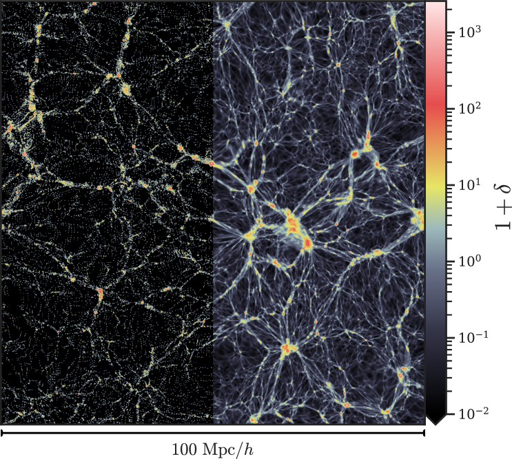
Figure 1: Slice through the overdensity field at $z=0$ of a standard $N$-body simulation (left half) and a simulation with discreteness reduction techniques applied (in each time step, as well as for the computation of the plotted density slice, right half). The particle and grid resolutions for both cases are $N=512^{3}$ and $M=1024^{3}$.

To control particle discreteness effects at the required level, we apply four important steps:

1. Increasing the number of gravity source particles (‘resampling’) by sheet interpolation during the force calculation (extending the quadratic interpolation of Ref. [38] to Fourier interpolation, see also [39])

2. Using higher-order mass-assignment schemes to represent particle positions more accurately [40] and deconvolving the density field on the grid with the mass assignment kernel

3. Using higher-order grid interlacing to suppress all low-order aliases (extending the interlacing of Ref. [26] to higher order)

4. Using the exact gradient kernel $\text{i}\bm{k}$ for the force calculation, rather than a finite difference gradient kernel.

The sheet interpolation has by far the largest effect in terms of suppressing discreteness. It harnesses the fact that for cold initial conditions, the phase-space density $f(t,\bm{x},\bm{p})$ in the Vlasov–Poisson equation (1) occupies a 3-dimensional manifold in the 6-dimensional phase space at all times $t$, the so-called Lagrangian submanifold. Hence, to increase the spatial resolution of the gravitational potential, we can ‘spawn’ new $N$-body gravity source particles in Lagrangian space on a much finer grid, determine their displacement by Fourier interpolation, and compute the resulting force on the $N$ particles using this refined potential field.

For illustration, Fig. 1 shows a plot of the $z=0$ density field with $N=512^{3}$ particles, evaluated on a grid with $M=1024^{3}$ cells, from a standard $N$-body simulation (left half) and a simulation with $5^{3}$-fold resampling of each particle for the density computation and the other discreteness reduction techniques applied in each simulation step (right half). The density field in the standard simulation is poorly sampled, particularly in underdense regions, with many cells containing no particles and hence $\delta_{N}=-1$. The resampling evidently suppresses discreteness and leads to a much more continuous density field. For a detailed explanation of each of these techniques, we refer to the Supplementary Material.

Initialising simulations without LPT.—

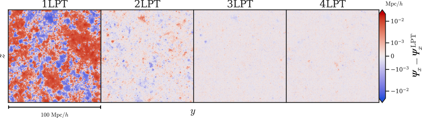
Figure 2: Residuals of the $x$-displacement ${\mathit{\Psi}}_{x}$ between our results with a single PowerFrog $N$-body step from redshift $z=\infty$ to $z=18$ and the corresponding LPT fields at $z=18$ for different LPT orders. Shown is a single slice in the Lagrangian $y$-$z$ coordinate plane.

We will now perform a single PowerFrog DKD time step starting from $z=\infty$ (i.e. $a=0$) to a redshift where one would typically initialise a cosmological simulation with 3LPT, namely $z=18$. We checked that the Jacobi determinant $\det\left(\differential\bm{x}^{\text{1LPT}}/\differential\bm{q}\right)>0$ for all particles at that time, and the standard deviation of the density field $\sigma(\delta^{\text{1LPT}})=0.30$. Hence, the entire simulation box is still in the single-stream regime, for which we have strong evidence that LPT converges [12, 15].

We consider the evolution of $N=512^{3}$ particles in a periodic simulation box of edge length $L=100\ \text{Mpc}/h$ subject to a flat $\Lambda$CDM cosmology with $\Omega_{m}=0.3$, $H_{0}=67.11\ \text{km}/\text{s}/\text{Mpc}$, $n_{s}=0.9624$, $\sigma_{8}=0.8$. We perform our computations on a single GPU, computing the forces with the particle-mesh (PM) method at mesh resolution $M=1024^{3}$.

Figure 2 depicts the residual between the 1-step $N$-body result and different LPT orders at $z=18$; specifically, we show a slice of the $x$-component of the displacement field ${\mathit{\Psi}}_{x}$ in the $y$-$z$ coordinate plane. In view of PowerFrog being designed to only match the 2LPT asymptote for $a\to 0$, it might be surprising that the 1-step $N$-body displacement field in fact lies even closer to 3LPT and 4LPT than to the 2LPT result. Intuitively, this can be understood by noting that the LPT terms are computed at the Lagrangian particle positions, i.e. by ‘pulling back’ the evolution of each particle to its initial location, whereas the kick in the $N$-body step updates the velocities at growth-factor time $\Delta D/2$ directly based on the potential that solves the Poisson equation at that time, which excites higher-order LPT terms. We leave a detailed analytical investigation of the higher-order contributions to future work.

We remark that also the velocity field is in good agreement with its LPT counterpart, see the Supplementary Material for details. The excellent match between the positions and momenta of a single PowerFrog step and high-order LPT makes the initialisation of cosmological simulations directly at the origin of time at $a=0$ with PowerFrog (or another integrator that follows the $\geq 2$LPT asymptotic behaviour for $a\to 0$) an attractive alternative to the traditional LPT-based computation of initial conditions.

We now study how the different discreteness reduction techniques affect the numerical solution of the $N$-body simulation. Figure 3 shows the relative root-mean-square (RMS) error of the displacement fields between a single $N$-body step from $z=\infty$ to $z=18$ using all discreteness suppression methods discussed above, together with the results when omitting one of these techniques at a time. Clearly, the sheet-based resampling of the density field is crucial for achieving convergence between $N$-body and LPT: without it, the residual towards LPT is entirely dominated by errors due to the particle-based approximation of the continuous density field at a level of 40%, and no differences between the different LPT orders are visible. The second-most important technique is the deconvolution of the density field with the mass assignment kernel, whose absence results in significant high-frequency noise that conceals the $3-4$LPT contributions in the residual. The residual also increases substantially when reducing the number of PM grid cells from $M=2^{3}N$ to $M=N$. The impact of using a higher-order mass assignment scheme (triangular-shaped cloud, TSC, instead of cloud-in-cell, CIC), of dealiasing the density field by means of interlaced grids, and of using the exact Fourier gradient kernel ${\rm i}\bm{k}$ instead of a 4${}^{\text{th}}$-order finite-difference gradient kernel is much more modest; however, leaving out any of these methods imprints a characteristic grainy structure in the $3-4$LPT residuals. With all techniques active, the 3LPT vs. 1-step PowerFrog residual is only 0.1%.

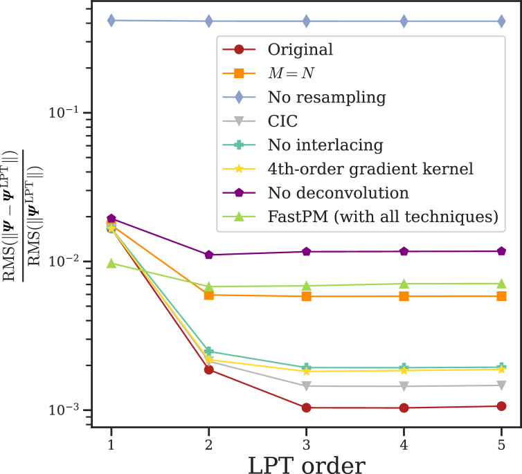
Figure 3: Relative root-mean-square error between the 1-step $N$-body simulation and different LPT orders at $z=18$ when using the PowerFrog integrator and applying all discreteness reduction techniques (‘Original’), when omitting one technique at a time, and when performing a FastPM DKD step instead of a PowerFrog step (applying all discreteness reduction techniques). Evidently, a carefully designed time integrator, resampling, deconvolution, and a fine PM grid (e.g. $M=2^{3}N$) are all necessary ingredients to access the $3-4$LPT regime.

Finally, the green triangles show the residual when performing a single step with the (DKD variant of the) FastPM stepper instead of PowerFrog which, recall, is consistent with the Zel’dovich approximation, but whose asymptotic behaviour for $a\to 0$ differs from 2LPT. Clearly, there is a significant 2LPT contribution in the residual, which prevails in the residuals w.r.t. higher LPT orders. A plot of the residual fields can be found in the Supplementary Material. FastPM is therefore not suitable as a 1-step initialiser of cosmological simulations.

In principle, it should be possible to construct integrators that match even higher LPT orders with a single time step by composing each step out of more than three drift/kick components, but since the gain from going beyond 3LPT can be expected to be small in practical applications, we leave an investigation in this direction to future work. Intuitively, one would expect to immediately see improvements when performing two or more steps to $z=18$. However, after the first step, the PowerFrog trajectory is already close to $3-4$LPT, the assumption that the time step starts in the asymptotic regime at $a\approx 0$ is no longer exactly valid, and no higher LPT knowledge is currently built into PowerFrog. Consequently, when increasing the number of time steps, we observe in our experiments that the match with $3-4$LPT may even slightly deteriorate at first, before convergence towards even higher orders can be seen. In future work, it would be interesting to make the time integrator adaptive such that the second step brings the numerical solution closer to $4-5$LPT, etc.

Analysis at $\bm{z=0}$.—

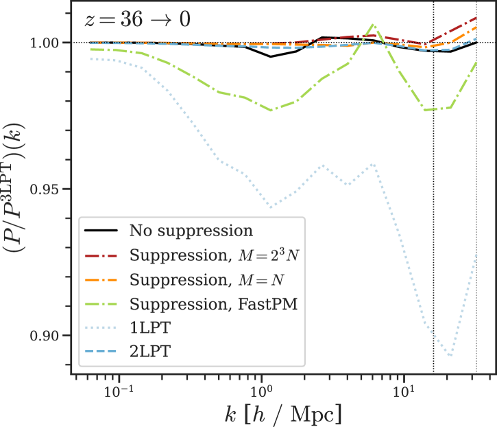
Figure 4: Power spectrum ratio at $z=0$ between cosmological simulations with 1LPT, 2LPT, or 1-step $N$-body initial conditions (with or without discreteness suppression) and 3LPT initial conditions. Even without any discreteness suppression, starting cosmological simulations with a single PowerFrog step from $z=\infty$ to $36$ and then continuing in standard $N$-body fashion leads to power spectrum errors $<1\%$ towards 3LPT on all scales. The dotted vertical lines show the Nyquist modes for $N=512^{3}$ and $M=1024^{3}$, respectively.

Finally, let us comment on the results one obtains when using the positions and momenta computed with a single PowerFrog step as the initial conditions for a (standard) cosmological simulation down to $z=0$. We take the same cosmology as in the previous section, $N=512^{3}$ particles, and initialise the simulations either with 1, 2, or 3LPT, or with a single $N$-body time step (that starts from $z=\infty$) at $z=36$; then, we run a cosmological simulation with the industry standard code Gadget-4 [42]. For the single $N$-body step, we consider PowerFrog (i) with discreteness suppression and grid sizes $M=512^{3}$ and $1024^{3}$, (ii) without any discreteness suppression and $M=512^{3}$, and (iii) a FastPM DKD step with discreteness suppression. Figure 4 shows the power spectrum ratio at $z=0$ w.r.t. the $3$LPT initial conditions, which we take as our reference. Interestingly, even without any discreteness suppression, the residual between the power spectra with PowerFrog and 3LPT initial conditions is $\leq 1\%$ on all scales. Also for the equilateral bispectrum, we find excellent agreement; however, the cross-spectrum drops significantly when omitting the discreteness reduction techniques (e.g. from $99\%$ to $93\%$ at the particle Nyquist frequency, see the Supplementary Material). This implies that in principle, standard $N$-body simulations can be started with a PowerFrog-like stepper without any discreteness suppression, and the resulting $z=0$ density field will be correct in terms of power spectrum and bispectrum, but its phases will be somewhat corrupted due to the discreteness noise.

Discussion.—

In this letter, we have provided the first demonstration of the field-level agreement between high-order LPT and cosmological $N$-body simulations in the single-stream regime. Choosing kinematic variables in which the solution remains regular in the limit $a\to 0$ allowed us to initialise simulations at the origin of time, making the customary LPT-based computation of the initial conditions at some scale factor $a>0$ obsolete—provided discreteness artefacts are sufficiently suppressed. Remarkably, the use of an LPT-informed time integrator implies that a single $N$-body time step starting from $a=0$ yields more accurate results than 2LPT, which is the established technique in the field for initialising cosmological simulations.

From a practical point of view, this opens up a wide range of applications: while the computational cost of the discreteness reduction techniques we applied to obtain the close match with LPT at early times shown in Fig. 2 is high, applying very few or even none of these techniques might give sufficiently accurate results in fast simulations and for analyses focused on late times (see the highly accurate power spectrum for ‘No suppression’ in Fig. 4). Although possibly slower than the $2-3$LPT computation, an $N$-body initialisation step from $a=0$ is superior in terms of memory requirements—no matter how fine the grid in Lagrangian space used for the resampling—as no large arrays need to be stored for each LPT order. Another interesting scope of application is given by zoom simulations, where the intricacies in the (usually FFT-based, but cf. [22] for 2LPT computed in configuration space) LPT computation arising from different resolutions can be circumvented.

In the era of precision cosmology, it is crucial to thoroughly test the agreement of complementary approaches to structure formation such as perturbative techniques and numerical methods and to clearly identify their range of validity (as well as their limitations). Our findings in this letter lay the groundwork for further comparison studies at the intersection between analytical and numerical methods.

I Asymptotics at the Big Bang Singularity, Perturbation Theory, and $N$-body Time Integration

Consider particle trajectories $a\mapsto\bm{X}(\bm{q},a)\in\mathbb{T}^{3}:=\mathbb{R}^{3}/\mathbb{Z}^{3}$ parameterised by the scale factor $a$ of the Universe and indexed by $\bm{q}\in\mathbb{T}^{3}$ (without loss of generality, this assumes units in which the boxsize is unity). For simplicity, let us assume Einstein-de Sitter asymptotics for $a\to 0$ in this section.

Following Ref. [43], the equations of motion can be written as

$$\frac{2a}{3}\frac{\differential^{2}\bm{X}}{\differential a^{2}}+\frac{\differential\bm{X}}{\differential a}+\bm{\nabla}_{\bm{x}}\phi(\bm{X},a) =0 1+\frac{a}{H_{0}^{2}}\Delta_{\bm{x}}\phi =1+\delta=\int_{\mathbb{T}^{3}}\differential^{3}q\;\delta_{D}(\bm{x}-\bm{X}(\bm{q},a)),$$ (S1)

where we defined the rescaled gravitational potential $\phi:=2\varphi/3$ for convenience.

I.1 Asymptotics for $\bm{a\to 0}$ and perturbation theory

In the limit $a\to 0$, the equations of motion (S1) impose the following asymptotic constraints (referred to as ‘slaving’ by [43])

$$\frac{\differential\bm{X}}{\differential a} \asymp-\bm{\nabla}_{\bm{q}}\phi_{\text{ini}} \delta \asymp 0\quad\Leftrightarrow\quad\bm{X}(\bm{q},a)\asymp\bm{q}$$ (S2)

as initial conditions, where $\phi_{\text{ini}}:=\phi(\bm{q},0)$. These initial constraints therefore require the density of the universe to become asymptotically uniform, and particle velocities to be of purely potential nature with a single scalar degree of freedom $\phi_{\text{ini}}$ remaining, which describes the entire initial condition of the universe. The $a\to 0$ asymptotics of the equations of motion therefore enforce the Zel’dovich approximation

$$\bm{X}(\bm{q},a)=\bm{q}-a\bm{\nabla}_{\bm{q}}\phi_{\text{ini}}+\mathcal{O}(a^{2})$$ (S3)

at leading order for $0\leq a\ll 1$.

At higher orders, it is customary in so-called Lagrangian perturbation theory (LPT) to expand the displacement field in terms of a Taylor series in time with space-dependent Taylor coefficients, i.e.

$$\bm{{\mathit{\Psi}}}(\bm{q},a):=\bm{X}(\bm{q},a)-\bm{q}=\sum_{n=1}^{\infty}\bm{\psi}^{(n)}(\bm{q})\;a^{n},$$ (S4)

for which all-order recursive relations are known [9, 10, 11] along with corrections for realistic $\Lambda$CDM cosmologies [27, 44].

LPT is by construction limited in its applicability to the regime $a<a_{\ast}$, where $a_{\ast}$ is the moment when particle trajectories overlap (i.e. the flow field becomes multi-kinetic). This moment is associated with sign-flips of the Jacobian of the Lagrangian map, i.e.

$$\det\left[\frac{\differential\bm{X}(\bm{q},a)}{\differential\bm{q}}\right]>0\quad\text{for all}\;\bm{q}\in\mathbb{T}^{3}\;\text{and}\;a<a_{\ast}.$$ (S5)

It is well known that LPT converges fairly quickly even at times close to $a_{\ast}$, which justifies the use of low-order LPT truncations [24, 15], except near regions that are very close to being spherically symmetric [45, 46, 47]. For this reason, it has been the method of choice to provide accurate initial conditions for cosmological simulations [48, 24].

A distinct disadvantage of (standard) LPT is that all evaluations of gravitational interactions must be carried out in Lagrangian space, requiring push forward of particles followed by pull back perturbative expansions. The distinct advantage of LPT over $N$-body simulations is however that the calculation is carried out in the fluid limit, i.e. the fluid elements are not discretised in principle. In practice, when used in the context of cosmological simulations, a discrete set of modes, truncated in the UV, is of course employed. Still, calculations [20, 21] and numerical experiments [22, 24] have shown that $N$-body simulations do not agree with the fluid-limit evolution. To remedy such effects, Ref. [22] has proposed to correct the particle motion at linear order for the error, while Ref. [24] has proposed to start simulations as late as possible from high-order LPT in order to suppress discreteness errors. Here we follow a distinctly different approach: we improve the simulations, both at the level of the time integration, as well as at the level of the force computation, in order demonstrate agreement. In the following sections, we detail the steps that are necessary to achieve this.

I.2 $\bm{N}$-body time integrators – symplectic and/or fast

In this section, we will provide some details on LPT-inspired integrators, focusing on relevant details for the PowerFrog integrator recently introduced in Ref. [25]. As discussed above, LPT expands the displacement field in Einstein-de Sitter cosmology in a Taylor series in terms of scale factor time $a$ in the pre-shell-crossing regime. This ansatz is readily carried over to an analogous series in terms of the linear growth-factor time $D$ for $\Lambda$CDM cosmology (neglecting higher-order correction terms derived in Ref. [27, 28]). In particular, in one dimension, all terms of the series with order $n\geq 2$ vanish, and only the Zel’dovich solution remains, i.e., $\bm{{\mathit{\Psi}}}(\bm{q},D)=-D\,\bm{\nabla}_{\bm{q}}\phi_{\text{ini}}$.

This suggests that employing the momentum w.r.t. $D$-time, $\bm{\mathit{\Pi}}=\differential\bm{X}/\differential D=\bm{P}/F$, for the time integration of cosmological $N$-body systems allows matching the dynamics on large scales to the Zel’dovich approximation or even higher LPT orders. Here, $\bm{X}$ and $\bm{P}=H(a)\,a^{3}\,\differential\bm{X}/\differential a$ denote the canonical position and momentum variable, respectively, and the factor relating $\bm{\mathit{\Pi}}$ and $\bm{P}$ is given by $F(a)=H(a)\,a^{3}\,\differential D/\differential a$ with the Hubble parameter $H(a)$.

In Ref. [25], we introduced so-called $\mathit{\Pi}$-integrators which implement this idea and advance the (non-canonical) position and momentum pair $(\bm{X}_{i},\bm{\mathit{\Pi}}_{i})$ for each particle $i$ from time step $k$ to $k+1$ via

$$\bm{X}_{i}^{k+\nicefrac{{1}}{{2}}} =\bm{X}_{i}^{k}+\frac{\Delta D}{2}\bm{\mathit{\Pi}}^{k}_{i},$$ (S6a)

$$\bm{\mathit{\Pi}}_{i}^{k+1} =p(D_{k},D_{k+1})\,\bm{\mathit{\Pi}}_{i}^{k}-q(D_{k},D_{k+1})\,a_{k+\nicefrac{{1}}{{2}}}\,\bm{\nabla}_{\bm{x}}\varphi_{N}(\bm{X}^{k+\nicefrac{{1}}{{2}}})_{i},$$ (S6b)

$$\bm{X}_{i}^{k+1} =\bm{X}_{i}^{k+\nicefrac{{1}}{{2}}}+\frac{\Delta D}{2}\bm{\mathit{\Pi}}^{k+1}_{i},$$ (S6c)

where $\varphi_{N}(\bm{X})$ is the gravitational potential induced by the $N$ simulation particles located at positions $\bm{X}$ via Poisson’s equation $\Delta_{\bm{x}}\varphi_{N}=3/(2a)\,H_{0}^{2}\,\Omega_{m}\,\delta_{N}$. Here, we defined $\Delta D=D_{k+1}-D_{k}$ as the length of the time step w.r.t. growth-factor time. The coefficient functions for the kick $p$ and $q$ can in principle be chosen independently; however, we showed in Ref. [25] that a $\mathit{\Pi}$-integrator reproduces the exact Zel’dovich solution in 1D until shell-crossing in a single time step if and only if $p$ and $q$ are related via

$$1-p=\frac{3}{2}\Omega_{m}\,H_{0}^{2}\,D_{k+\nicefrac{{1}}{{2}}}\,q.$$ (S7)

Also, we showed that the only symplectic integrator that satisfies aforementioned relation is the well-known FastPM integrator by Ref. [29], which corresponds to the choice $p(D_{n},D_{n+1})=F(D_{n})/F(D_{n+1})$. However, in view of the expansion of the universe, it is questionable whether symplecticity is a necessary property for time integrators when considering large scales where the particle motion is largely governed by the Hubble flow. Indeed, we introduced new (non-symplectic) integrators in Ref. [25], which perform better than FastPM in terms of the power spectrum and cross-spectrum for any given number of time steps. One of these integrators, which we named PowerFrog, is explicitly constructed to match the 2LPT asymptote at early times $a\to 0$. For a single time step starting from $D(a=0)=0$ to some final growth-factor time $\Delta D$, the coefficient functions $p(0,\Delta D)$ and $q(0,\Delta D)$ of PowerFrog are simply given by

$$p(0,\Delta D)=-\frac{5}{7},\qquad q(0,\Delta D)=\frac{16}{7\,\Omega_{m}\,H_{0}^{2}\,\Delta D}.$$ (S8)

For later times $D_{k}>0$, the function $p(D_{k},D_{k+1})$ in the kick takes the form

$$p(D_{k},D_{k+1})=\frac{\alpha D_{k}^{\epsilon}+\beta D_{k+1}^{\epsilon}}{D_{k+\nicefrac{{1}}{{2}}}^{\epsilon}}+\gamma,$$ (S9)

where the coefficients $\alpha,\beta,\gamma,\epsilon$ need to be determined numerically as the solution of a transcendental system of equations that ensures (global) second-order convergence (eliminating three degrees of freedom) and consistency with the 2LPT asympote (eliminating the fourth degree of freedom), see Ref. [25]. The coefficient $q$ then follows from Eq. (S7).

II Particle discreteness reduction in cosmological particle-in-cell codes

The main limitation in the convergence of $N$-body simulations to the fluid limit is due to the finite sampling by particles. In simulations, the continuous indexing by the Lagrangian coordinate $\bm{q}\in\mathbb{T}^{3}$ is replaced by a discrete collection of characteristics, which we initially arrange in terms of a simple cubic lattice $\bm{q}_{\bm{i}}:=\bm{i}/\mathcal{N}$ where $\bm{i}\in\mathbb{I}_{N}:=(\mathbb{Z}/\mathcal{N})^{3}$. Here, $\mathcal{N}$ is the linear number of particles, i.e. $\mathcal{N}^{3}=N$. In particular, we then have a discrete set of particle trajectories $a\mapsto\bm{X}_{\bm{i}}(a):=\bm{X}(\bm{q}_{\bm{i}},a)$ along with their displacement vectors $\bm{{\mathit{\Psi}}}_{\bm{i}}(a):=\bm{X}_{\bm{i}}(a)-\bm{q}_{\bm{i}}$. We distinguish between active ‘characteristic’ particles and passive ‘mass’ carrying particles. In standard particle-in-cell (PIC) / PM simulations, these two particles are identical. We shall clarify this distinction in what follows.

II.1 Spectral sheet interpolation

As described above, due to its cold nature, CDM occupies only a three-dimensional submanifold of phase space. This property can be exploited to interpolate the displacement field to new mass resolution elements [49, 50] in order to approach the continuum limit. This has already been used for ‘sheet-based’ simulations [51, 38, 52] that are known to overcome some of the well-known discreteness problems of cold gravitational $N$-body simulations, such as artificial fragmentation. While previous work in this direction has mostly employed low-order interpolation on the Lagrangian submanifold (tetrahedral [49, 50, 51, 52], tri-linear, tri-quadratic [38]), here we use Fourier interpolation to achieve spectral accuracy (see also [39]). To this end, we define the Fourier-space translation operator

$$\hat{T}_{\bm{y}}f(\bm{x}):=f(\bm{x}+\bm{y})=\mathcal{F}^{-1}\left[{\rm e}^{{\rm i}\bm{k}\cdot\bm{y}}\mathcal{F}[f]\right](\bm{x}),$$ (S10)

implemented with a discrete Fourier transform. Given a Lagrangian shift vector $\bm{s}$ and our set of active characteristic particles, we can then generate new sets of sheet-interpolated ‘mass’ particles by evaluating

$$\bm{X}^{\bm{s}}(\bm{q}_{\bm{i}},a):=\bm{q}_{\bm{i}}+\bm{s}+\hat{T}_{\bm{s}}{\mathit{\Psi}}(\bm{q}_{i},a).$$ (S11)

As the particles are occupying a simple cubic lattice, we have the invariance $\bm{X}^{\bm{i}^{\prime}/\mathcal{N}}(\bm{q}_{\bm{i}},a)=\bm{X}(\bm{q}_{\bm{i}-\bm{i}^{\prime}},a)$. By choosing subdivisions of the unit cube, we can upsample the particle distribution $R$ times per dimension, i.e. $\bm{s}=\bm{m}/(\mathcal{N}R)$ where $\bm{m}\in[0,1,\dots,R-1]^{3}$.

II.2 Mass assignment / interpolation kernels

In PIC/PM codes, the initial distribution function $f_{\text{ini}}(\bm{x},\bm{p})$ is sampled by the $N$ active characteristic particles. As described above, we allow for upsampling them to a larger number of $N_{\text{mass}}\geq N$ passive mass particles,

$$\hat{n}(\bm{x},a):=\frac{1}{N_{\text{mass}}}\sum_{j=1}^{N_{\text{mass}}}\delta_{D}(\bm{x}-\bm{X}_{j}(a)).$$ (S12)

The particle mesh is given by the 3-dimensional Dirac comb of uniform spacing $h>0$, i.e. the object

$${}_{h}(\bm{x}):=\sum_{\bm{n}\in\mathbb{Z}^{3}}\delta_{D}(\bm{x}-h\bm{n}).$$ (S13)

Given a mass assignment kernel (MAK) $W(\bm{x})$, the grid-interpolated particle distribution can be written as [26]

$$\mathfrak{n}(\bm{x},a):={}_{h}(\bm{x})\,\left(\hat{n}(\bm{x},a)\ast W(\bm{x})\right),$$ (S14)

where the asterisk denotes convolution. MAKs of order $n$ are generated by $n$ convolutions of the box function with itself, i.e.

$$W_{\rm NGP}(x):=W_{1}(x) =\frac{1}{h}\left\{\begin{array}[]{ll}1&\quad\textrm{for }\left|x\right|\leq\frac{h}{2}\\ 0&\quad\textrm{otherwise}\end{array}\right.$$ (S15c)

$$W_{\rm CIC}(x):=W_{2}(x) =\frac{1}{h}\left\{\begin{array}[]{ll}1-\frac{\left|x\right|}{h}&\quad\textrm{for }\left|x\right|<h\\ 0&\quad\textrm{otherwise}\end{array}\right.$$ (S15f)

$$W_{\rm TSC}(x):=W_{3}(x) =\frac{1}{h}\left\{\begin{array}[]{ll}\frac{3}{4}-\left(\frac{x}{h}\right)^{2}&\quad\textrm{for }\left|x\right|\leq\frac{h}{2}\\ \frac{1}{2}\left(\frac{3}{2}-\frac{\left|x\right|}{h}\right)^{2}&\quad\textrm{for }\frac{h}{2}\leq\left|x\right|<\frac{3h}{2}\\ 0&\quad\textrm{otherwise}\end{array}\right.$$ (S15j)

$$W_{\rm PCS}(x):=W_{4}(x) =\frac{1}{h}\left\{\begin{array}[]{ll}\frac{1}{6}\left[4-6\left(\frac{x}{h}\right)^{2}+3\left(\frac{|x|}{h}\right)^{3}\right]&\quad\textrm{for }\left|x\right|\leq h\\ \frac{1}{6}\left(2-\frac{\left|x\right|}{h}\right)^{3}&\quad\textrm{for }h\leq|x|<2h\\ 0&\quad\textrm{otherwise}\end{array}\right.$$ (S15n)

where the three-dimensional version is simply given by the product of three one-dimensional kernel evaluations. While most cosmological simulations use $$n=2 n=3 n=4$$ (CIC), we used (TSC) to sufficiently reduce particle discreteness effects for our precision study. We also experimented with (PCS), which gave a very slight additional improvement over TSC in terms of the residuals towards LPT; however not enough to warrant the increased runtime (in particular given that other discreteness reduction techniques are much more significant, see Fig. 3), for which reason we present the TSC-based results herein. Note that Ref. [40] lists kernels of even higher order, which we did however not use. They have the Fourier transform

$$\widetilde{W}_{n}(k)=\left[{\rm sinc}(hk/2)\right]^{n}.$$ (S15o)

II.3 Poisson solver

We use an FFT-based spectral Poisson solver. Given the discretised mass distribution on the grid from Eq. (S14), we obtain the acceleration field as

$$\bm{\mathfrak{a}}(\bm{x}):=\mathcal{F}^{-1}\left[-\frac{{\rm i}\bm{k}}{\|\bm{k}\|^{2}}\;\widetilde{W}_{n}^{-2}(\bm{k})\;\;\mathcal{F}[\mathfrak{n}](\bm{k})\right]\,,$$ (S16)

where $\mathfrak{n}$ is defined in Eq. (S14). The acceleration field is then interpolated back to the active particle positions using once more the $W$ kernel. The double deconvolution with the MAK $W$ accounts for both the deposit and the back-interpolation to the active particles.

Instead of solving the Poisson equation in Fourier space (where the discretisation occurs at the level of the FFT, which only takes into account a finite number of modes), it is also common practice to compute the derivatives in real space using finite-difference (FD) approximations. For instance, the popular Gadget-2 code [53] uses a fourth-order stencil for the gradient whose Fourier transform is given by

$$\mathcal{F}[\partial_{x_{d}}](\bm{k})=\frac{{\rm i}}{6}\left(8\sin(k_{d})-\sin(2k_{d})\right),\qquad\text{for }d\in\{1,2,3\},$$ (S17)

where $\bm{k}=(k_{1},k_{2},k_{3})^{\top}$ is in units of the grid’s Nyquist wavenumber. In our ablation study, we analyse the effect of replacing the spectral ${\rm i}\bm{k}$ gradient kernel by this commonly employed fourth-order FD approximation; however, we still perform the differentiation in Fourier space (as done in e.g. Ref. [29]). Note that due to the odd symmetry of FD stencils for the gradient, their Fourier transform is given by the sum of sines, which must vanish at the Nyquist wavenumber (see the discussion in Ref. [54, Sec. 3.4]). The FD gradient operators therefore effectively act as low-pass filters, which suppress power close to the Nyquist frequency.

While the situation is, in principle, similar for the Laplacian operator (with FD approximations giving rise to a truncated cosine series in Fourier space), we noticed very little difference when replacing the spectral Laplacian $-k^{2}$ by FD operators, for which reason we do not include any ablation tests for the Laplacian herein.

II.4 Dealiasing by interlacing

PIC/PM simulations suffer from aliasing since the particle distribution is not band limited. Aliasing could in principle be reduced by increasing the sampling rate, i.e. resolution of the mesh, which is however prohibitive due to its memory requirements. It is well known that interlacing techniques can be used to eliminate the dominant aliases and effectively achieve sampling comparable to higher resolution. Here, we adopt the technique proposed by Ref. [55] (see also [26, 56]) and use interlaced grids in order to remove the dominant aliasing contributions in the accelerations.

It is easy to show (e.g. [26, Sec. 7.8]) that by depositing the particles onto a grid ${}_{h}^{(\nicefrac{{1}}{{2}},\nicefrac{{1}}{{2}},\nicefrac{{1}}{{2}})}$ that is shifted by half a grid-cell w.r.t. the original grid _h, i.e.

$${}_{h}^{(\nicefrac{{1}}{{2}},\nicefrac{{1}}{{2}},\nicefrac{{1}}{{2}})}(\bm{x}):=\sum_{\bm{n}\in\mathbb{Z}^{3}}\delta_{D}\left(\bm{x}-h\left(\bm{n}+(\nicefrac{{1}}{{2}},\nicefrac{{1}}{{2}},\nicefrac{{1}}{{2}})^{\top}\right)\right),$$ (S18)

and averaging the two accelerations resulting from the grids _h and ${}_{h}^{(\nicefrac{{1}}{{2}},\nicefrac{{1}}{{2}},\nicefrac{{1}}{{2}})}$, half of the aliases can be removed (namely those for which $n_{1}+n_{2}+n_{3}=\text{odd}$, where $\bm{n}=(n_{1},n_{2},n_{3})^{\top}$ now indexes the reciprocal lattice). The resulting checkerboard pattern on the reciprocal lattice is illustrated in the first panel of Fig. S1 (in 2D for illustrative purposes), with aliased (dealiased) Brillouin zones shown in black (white). By extending this idea to more than two shifted grids, higher-order alias contributions can be removed, see the second and third panel in Fig. S1.

In practice, given a set of shift vectors $\mathcal{D}=\{\bm{d}_{1},\ldots,\bm{d}_{D}\}$ with $\bm{d}_{i}\in[0,1)^{3}$ for $i\in\{1,\ldots,D\}$, we implement the interlacing as follows:

for $\bm{d}\in\mathcal{D}$ do

       Compute the (resampled) overdensity according to Eq. (S14) on the shifted grid ${}_{h}^{\bm{d}}(\bm{x})$;

       Solve the Poisson equation and obtain the acceleration field $\bm{\mathfrak{a}}(\bm{x})$ on the grid via Eq. (S16);

       Interpolate the accelerations back to the particles, using the same MAK $W(\bm{x})$;

      

Average the accelerations over all interlaced grids $\mathcal{D}$;

Of course, it is not necessary to store the accelerations for each grid in memory, but one can simply add the new to the currently stored accelerations in each loop iteration and divide the final result by $D$ to obtain the dealiased acceleration field.

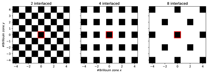
Figure S1: Removal of aliases with increasingly higher-order interlacing schemes. While our simulations are three-dimensional, the procedure is shown here for two dimensions for illustrative purposes. The left panel illustrates the standard approach of interlacing two grids [26, 56]—shifted by $(\nicefrac{{h}}{{2}},\nicefrac{{h}}{{2}})$ w.r.t. each other—which removes every second alias and therefore the dominant aliasing contribution (removed aliases are white). This procedure can be continued to four interlaced grid removing increasingly more aliases by including also the shifts $(\nicefrac{{h}}{{2}},0)$ and $(0,\nicefrac{{h}}{{2}})$ (middle panel), or to eight interlaced grids, where further $h(\nicefrac{{1}}{{2}}\pm\nicefrac{{1}}{{4}},\nicefrac{{1}}{{2}}\pm\nicefrac{{1}}{{4}})$ are included. The red cell indicates the first Brillouin zone at $(0,0)$ in each case.

II.5 Specific discreteness reduction parameters for the PowerFrog step from $\bm{z=\infty}$

Having explained the different discreteness suppression techniques, we can now summarise the specific settings we used when performing a PowerFrog step from $z=\infty$ to $z=18$ in order to achieve the small residuals towards $3-4$LPT (see Fig. 2):

• Spectral sheet interpolation for spawning $5^{3}$ ‘mass’ particles from each ‘characteristic’ particle (i.e. $R=5$), based on which the density field is computed

• TSC mass assignment

• Dealiasing by using $D=16$ interlaced grids (the resulting Brillouin pattern is the 3D counterpart of the one for the ‘8 interlaced’ case in 2D shown in Fig. S1)

• Exact spectral gradient kernel (${\rm i}\bm{k}$) and double deconvolution with the MAK when solving Poisson’s equation.

III Additional material for the discreteness-suppressed PowerFrog step from $\bm{z=\infty}$

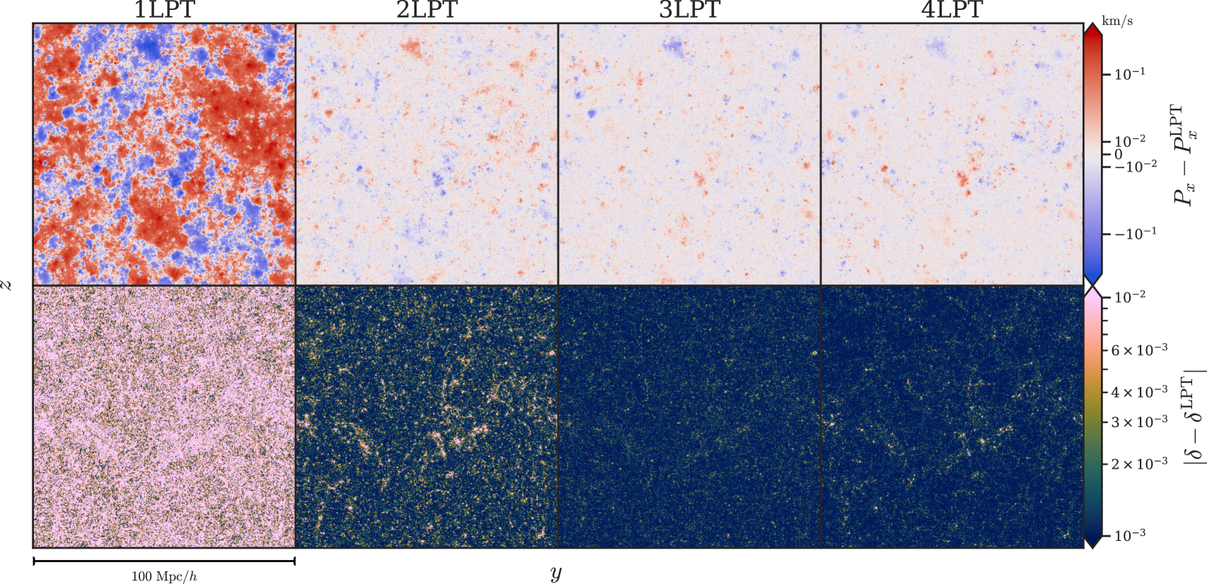
Figure S2: Residuals of the Lagrangian (comoving) $x$-velocity $P_{x}$ (top) and the density contrast $\delta$ (bottom) between our results with a single PowerFrog step from $z=\infty$ to $z=18$ and the corresponding LPT fields at $z=18$ for different LPT orders (see Fig. 2 in the main body for the displacement residual). Shown is a single slice in the $y$-$z$ plane.

For completeness, we show the velocity and density residuals after a single PowerFrog step from $z=\infty$ to $z=18$ w.r.t. different LPT orders in Fig. S2 (cf. Fig. 2 in the main body for the residual of the displacement field). Since the displacement field lies much closer to $3-4$LPT than to 2LPT, the same is true for the density field. In contrast, the velocity residual towards 3LPT is only slightly smaller than towards 2LPT. This might be related to the fact that the single PowerFrog step consists of two drifts (i.e. positions updates), but only one kick (i.e. velocity update).

IV Additional material for the ablation study

In Fig. 3 in the main body of this work, we studied the effect of the different discreteness reduction techniques on the relative RMS error between the single-step displacement field at $z=18$ and different LPT orders. To provide a more intuitive understanding of these errors, we plot the displacement field residuals for the different cases in Fig. S3.

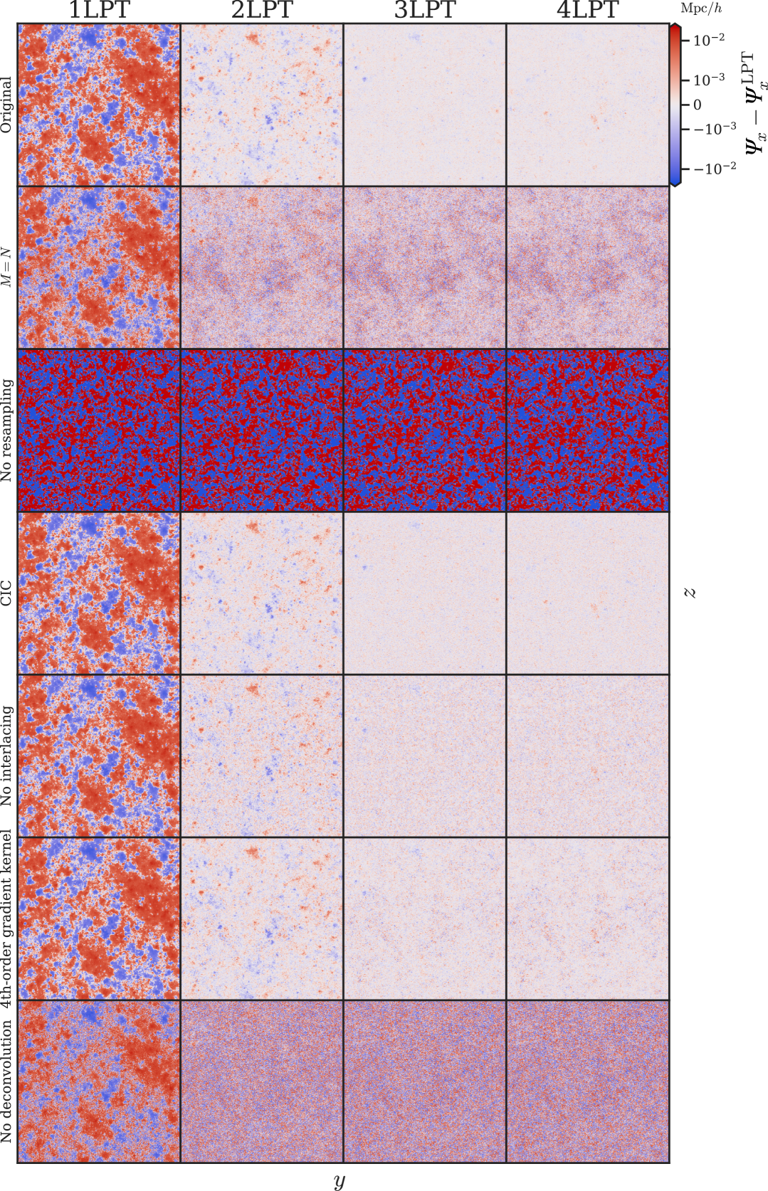
Figure S3: Residuals of the $x$-displacement ${\mathit{\Psi}}_{x}$ between our results with a single step from $z=\infty$ to $z=18$ and the corresponding LPT fields at $z=18$ for different LPT orders (columns) when omitting one discreteness suppression technique at a time (rows). Shown is a single slice in the $y$-$z$ plane.

The first row shows again the residual of the displacement fields between a single $N$-body step from $z=\infty$ to $z=18$ with the PowerFrog stepper, using all discreteness suppression methods discussed above (i.e. the same results as Fig. 2). Each subsequent row depicts the results when omitting one of these techniques at a time. As discussed in the main text, the sheet-based resampling has by far the biggest impact, followed by the deconvolution of the mass assignment kernel, and using a PM mesh at twice the particle resolution, i.e. $M=2^{3}N$, rather than $M=N$. The other techniques have a smaller effect; however, each of them contributes to reducing the discreteness noise in the ‘Original’ row, where the $3-4$LPT residual is clearly dominated by patch-like structures, rather than high-frequent noise. These patches stem from the fact that—as expected—the single PowerFrog step does not entirely capture the $3-4$LPT terms, for which reason they cannot be removed by suppressing discreteness even further. In future work, it would also be interesting to implement PowerFrog into a cosmological simulation code that computes nearby forces by means of a tree or even direct summation and to study how this affects the residuals towards LPT.

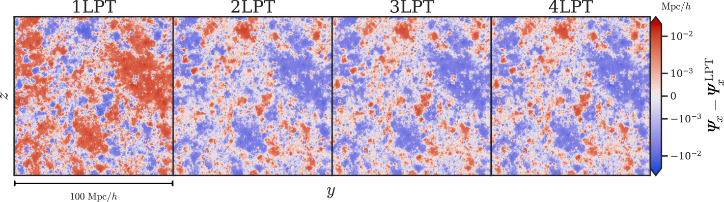
Figure S4: Same as Fig. 2 in the main body, but with a single DKD step of the FastPM integrator rather than PowerFrog. Evidently, a single FastPM step does not correctly capture the 2LPT term.

We also repeat the 1-step simulation from $z=\infty$ with the popular FastPM integrator [29], which correctly reproduces the 1LPT (i.e. Zel’dovich) growth, but has asymptotics different from 2LPT for $z\to\infty$. While FastPM is often employed in kick-drift-kick form, we perform a single drift-kick-drift step here, noting that the acceleration at $z=\infty$ vanishes for particles placed on a homogeneous grid, for which reason starting with a kick at $z=\infty$ would be futile. Figure S4 shows a slice of the residual between the 1-step FastPM simulation and different LPT orders (cf. Fig. 2 in the main body for the same plot with the PowerFrog stepper). Clearly, there is a significant 2LPT contribution in the residual, which is also present in the residuals w.r.t. higher LPT orders (see Fig. 3 for a quantitative assessment). FastPM should therefore not be used for initialising cosmological simulations in a single step from $z=\infty$, just as any other integrator that is merely ‘Zel’dovich-consistent’ in the sense of Def. 3 in Ref. [25]. We remark, however, that PowerFrog is not the only possible choice for an integrator with correct 2LPT asymptotics, and one can in principle construct integrators whose behaviour for $z\to\infty$ explicitly matches higher LPT orders $>2$.

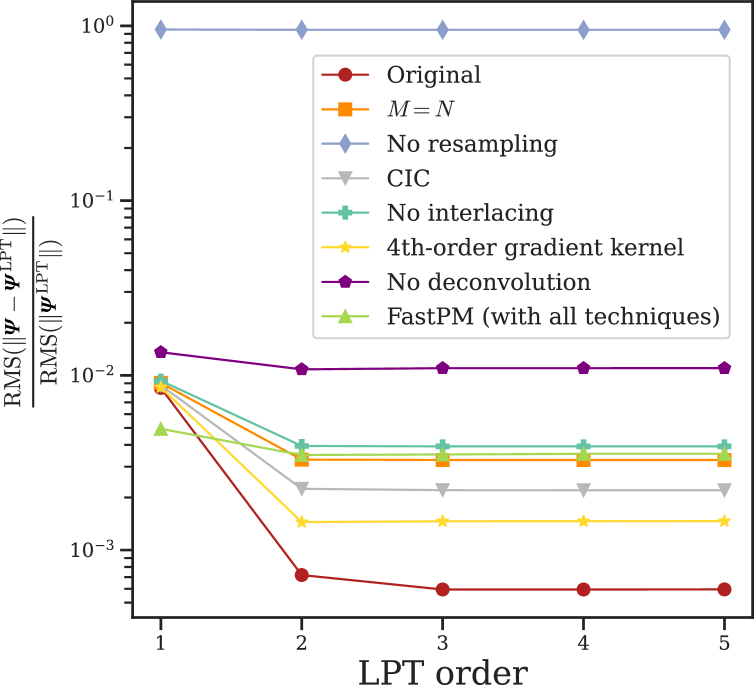
Figure S5: Same as Fig. 3, but for a single step from $z=\infty$ to $z=36$ instead of $z=18$: relative RMS error between the 1-step $N$-body simulation and different LPT orders when using the PowerFrog integrator and applying all discreteness reduction techniques (‘Original’), when omitting one technique at a time, and when performing a FastPM DKD step instead of a PowerFrog step (applying all discreteness reduction techniques).

Finally, we study how the impact of the different discreteness suppression techniques varies when changing the end time of the single $N$-body step. Figure S5 shows again the RMS errors when omitting each discreteness suppression technique at a time when performing a single time step from $z=\infty$, but now to $z=36$ instead of $z=18$ as shown in Fig. 3 in the main body. Going to this higher redshift affects the order of importance of the different techniques: while the resampling followed by the deconvolution still have the largest effect, omitting the interlaced grid to alleviate aliasing and using CIC instead of TSC mass assignment instead of TSC now lead to a much larger error, reflecting the increased need to suppress discreteness effects at early times. When applying all techniques, the relative error between a single PowerFrog step and 3LPT at $z=36$ is $<0.06\%$. Since the 3LPT contribution at $z=36$ is still small, so is the difference between the 2LPT and 3LPT residuals for the ‘Original’ case.

V Additional results at late times

In the main body, we used the particle positions and momenta computed with a single PowerFrog step from $z=\infty$ to $z=36$ as initial conditions for a standard $N$-body simulation with the Gadget-4 simulation code and compared the resulting power spectrum at $z=0$ to its counterparts from LPT-initialised simulations. We found that even if no discreteness suppression techniques are employed for the initialisation step, the power spectra agree to within $1\%$ on all scales (see Fig. 4). However, the power spectrum alone is not a sufficient statistic for determining if the quality of the $z=0$ field computed with the PowerFrog initial conditions is satisfactory.

Figure S6 shows the (normalised) cross-spectrum for each simulation w.r.t. the 3LPT-initialised simulation, which we take as our reference. Unlike for the power spectrum, the impact of the discreteness suppression on the cross-spectrum is significant: omitting the discreteness suppression causes a drastic drop in cross-power on small scales, comparable in magnitude to the impact of using FastPM instead of PowerFrog (while keeping all discreteness suppression techniques). This implies that the coherence between the discrete and continuous phases is irretrievably corrupted by the discreteness. As a further check, we plot the equilateral bispectra in the right panel of Fig. S6. As for the power spectra, all PowerFrog-initialised simulations yield results very similar to the 2LPT case, although the bispectrum is somewhat noisier for the non-suppressed PowerFrog initial conditions.

To study the time dependence of these statistics, we also show a plot of the results at $z=3$. Also here, the agreement between the power spectra with 1-step PowerFrog initial conditions and with 3LPT is excellent—regardless of the discreteness suppression—and superior to the 2LPT initial conditions, which entail a slight suppression of power on small scales due to transients that have not fully decayed by $z=3$. Similar to the $z=0$ case, the equilateral bispectra match well; however, the cross-spectrum is strongly affected by the discreteness noise on small scales.

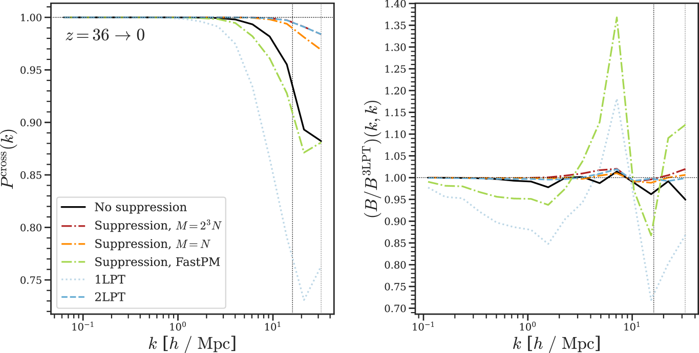
Figure S6: Cross-power spectrum (left) and equilateral bispectrum ratio (right) between the $z=0$ density fields with initial conditions generated at $z=36$ (either with LPT or with a single $N$-body step from $z=\infty$) w.r.t. 3LPT initial conditions. The same plot for the power spectrum is shown in Fig. 4 in the main part.

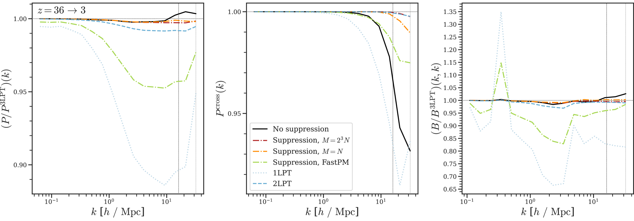
Figure S7: Same statistics as in Figs. 4 and S6, but evaluated at $z=3$.