A dynamic mean-field statistical model of academic collaboration

Abstract.

There is empirical evidence that collaboration in academia has increased significantly during the past few decades, perhaps due to the breathtaking advancements in communication and technology during this period. Multi-author articles have become more frequent than single-author ones. Interdisciplinary collaboration is also on the rise. Although there have been several studies on the dynamical aspects of collaboration networks, systematic statistical models which theoretically explain various empirically observed features of such networks have been lacking. In this work, we propose a dynamic mean-field model and an associated estimation framework for academic collaboration networks. We primarily focus on how the degree of collaboration of a typical author, rather than the local structure of her collaboration network, changes over time. We consider several popular indices of collaboration from the literature and study their dynamics under the proposed model. In particular, we obtain exact formulae for the expectations and temporal rates of change of these indices. Through extensive simulation experiments, we demonstrate that the proposed model has enough flexibility to capture various phenomena characteristic of real-world collaboration networks. Using metadata on papers from the arXiv repository, we empirically study the mean-field collaboration dynamics in disciplines such as Computer Science, Mathematics and Physics.

1. Introduction

There is empirical evidence that collaboration in academia has significantly increased during the last two decades. Advancements in communication and technology may be one of the main reasons. Multi-author articles have become more frequent than single-author articles. Collaboration between different disciplines is also on the rise (Porter and Rafols, 2009). Quantitative study of collaboration has therefore attracted a great deal of attention and there is already a substantial body of (mostly empirical) work analyzing various aspects of collaboration, both intra- and inter-disciplinary. An incomplete list of relevant works include Lawani (1980); Subramanyam (1983); Ajiferuke et al. (1988); De Lange and Glänzel (1997); Newman (2001); Bettencourt et al. (2008, 2009); Porter and Rafols (2009); Tomasello et al. (2017); Abramo et al. (2018); Liang et al. (2018); Lalli et al. (2020); Hurtado-Marín et al. (2021); Ebrahimi et al. (2021).

Despite the large body of existing works, there is a shortage of flexible statistical generative models which are capable of capturing various empirically observed features of real-world collaboration networks and are accompanied by statistical estimation/inference frameworks that enjoy rigorous theoretical guarantees. In this work, we attempt to address this gap and propose a dynamic mean-field model which takes into consideration several aspects of scientific collaboration, such as the temporal intensity of producing research articles and the role of past collaboration while selecting new collaborators. The proposed model is mean-field in the sense that we only consider the collaboration dynamics of a typical author in a pool of researchers. We develop both parametric and non-parametric frameworks for estimating the model parameters and establish consistency and asymptotic normality results for the proposed estimators.

As a first step, we primarily focus on how the degree of collaboration of a typical author, rather than the local structure of her collaboration network, changes over time. We consider several popular indices of collaboration from the literature (Lawani, 1980; Subramanyam, 1983; Ajiferuke et al., 1988) and study their dynamics under the proposed model. In particular, we obtain exact formulae for the expectations and temporal rates of change of these indices. Through extensive simulation experiments, we demonstrate that the proposed model has enough flexibility to capture various phenomena characteristic of real-world collaboration networks. Using metadata on papers from the arXiv repository (Clement et al., 2019), we empirically study the mean-field collaboration dynamics in disciplines such as Computer Science, Mathematics and Physics.

The rest of the paper is organised as follows. In Section 2.1 we describe the proposed mean-field model. Section 2.2 then describes our estimation framework. In Section 3, we discuss several metrics of collaboration. In Section 4 we describe our main theoretical findings. The proofs are deferred to the appendix. In Section 5 we describe some simulation experiments. Then in Section 6, we describe an analysis of Computer Science, Mathematics and Physics papers from the arXiv repository. Section 7 is the final section with some concluding remarks and directions for future work.

2. Set-up and methodology

2.1. The proposed model

Let us denote the authors by $\mathcal{A}=\{a_{0},\ldots,a_{L}\}$. Fix an individual author, say $a_{0}$. We assume that $a_{0}$ writes papers at events of an inhomogeneous Poisson process with intensity functional $\lambda(t)$. We denote the event-times of this process by $E_{n},n\geq 1$. Further, we assume that she writes exactly one paper at each event. Recall that the total number of events $N[s,t]$ during interval $[s,t]$ is then a $\mathsf{Poisson}(\int_{s}^{t}\lambda(u)\,du)$ random variable. This is simply the total number of papers that $a_{0}$ has written during the interval $[s,t]$. We denote by $\mathcal{C}_{n}$ the set of co-authors of $a_{0}$ at event $E_{n}$. Also, for $i\in[L]:=\{1,\ldots,L\}$, set

$$m_{n,i}=\sum_{\ell=1}^{n}\mathbf{1}_{\mathcal{C}_{\ell}}(i),$$

which is the number of papers $a_{0}$ has co-authored with $a_{i}$ by event $E_{n}$. Clearly, $0\leq m_{n,i}\leq n$. We set $m_{0,i}=0$ for all $i\in[L]$. Given $\mathcal{C}_{1},\ldots,\mathcal{C}_{n}$, at event $E_{n+1}$ a new paper is written in the following way:

1. For any $i\in[L]$,

   $$\mathbf{1}_{\mathcal{C}_{n+1}}(i)\mid\mathcal{C}_{1},\ldots,\mathcal{C}_{n}\sim\mathsf{Bernoulli}(F_{n+1}(m_{n,i})),$$ (1)

   where $F_{n+1}:\{0\}\cup\mathbb{N}\rightarrow[0,1]$. Since $m_{n,i}\leq n$, we take $F_{n+1}$ to be supported on $\{0\}\cup[n]$.

2. Given $\mathcal{C}_{1},\ldots,\mathcal{C}_{n}$, co-authors are included in $\mathcal{C}_{n+1}$ independently of each other, i.e. the indicators $\{\mathbf{1}_{\mathcal{C}_{n}}(i)\}_{i\in[L]}$ are conditionally independent given $\mathcal{C}_{1},\ldots,\mathcal{C}_{n}$.

Thus, $\#\mathcal{C}_{n+1}\mid\mathcal{C}_{1},\ldots,\mathcal{C}_{n}$ is a sum of $L$ independent Bernoulli variables with parameters $F_{n+1}(m_{n,i}),i\in[L]$. A cartoon of event $E_{n+1}$ is shown in Figure 1.

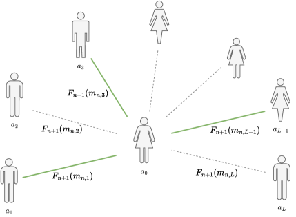
Figure 1. A cartoon of the $(n+1)$-the paper writing event for author $a_{0}$: Solid green lines indicate co-authorship; thus $\mathcal{C}_{n+1}=\{a_{1},a_{3},a_{L-1}\}$.

Note that in the above model, there are two (infinite dimensional) unknown parameters which have to be estimated: the intensity functional $\lambda(t)$ of the paper writing process $N$, and the event-specific co-authorship probabilities $\{F_{n}(k)\}_{n\geq 1,k\geq 0}$. One may of course consider parametric sub-models. For instance, for short intervals of time, one may use a homogeneous Poisson process, thereby reducing the intensity functional to a scalar parameter $\lambda>0$. More importantly, one parametric model for $F_{n}(k)$ that we will be of particular interest to us is the following:

$$F_{n}(k)=\begin{cases}a_{n}k+b_{n}&\text{if }0\leq k\leq n-1,\\ 0&\text{otherwise},\end{cases}$$ (2)

where $a_{n}$ and $b_{n}$ are unknown parameters. Since $F_{n}$ is supported on $\{0\}\cup[n-1]$, we must have that $b_{n}=F_{n}(0)\in[0,1]$ and for $n\geq 2$, $-\frac{b_{n}}{n-1}\leq a_{n}\leq\frac{1-b_{n}}{n-1}$.

Our main objects of interest will be the observables $X_{k}[s,t]=$ the number of $k$-author papers written by $a_{0}$ during $[s,t]$, $k\geq 1$. Notice that

$$X_{k}[s,t]=\sum_{n\geq 1}\mathbb{I}(\#\mathcal{C}_{n}=k-1)\mathbf{1}_{[s,t]}(E_{n})$$

and

$$\sum_{k\geq 1}X_{k}[s,t]=N[s,t]\sim\mathsf{Poisson}\bigg{(}\int_{s}^{t}\lambda(u)\,du\bigg{)}.$$

2.2. Estimation framework

We now discuss non-parametric estimation of the parameters $\lambda(t)$ and $(F_{n}(k))_{n\geq 1,k\geq 0}$. We also consider estimation of $F_{n}(k)$ under the parametric sub-model described in (2).

2.2.1. Estimation of the intensity functional $\lambda(t)$.

Since we usually have knowledge of approximately when an article is written (e.g., when a paper is first submitted to a journal, or uploaded to a repository such as the arXiv), it is reasonable to assume that we know the timings of the paper writing events $E_{n}$. Thus we may employ standard techniques for estimating intensity functionals of Poisson processes to estimate $\lambda(t)$. In this article, we will use the kernel smoothing approach of Diggle (1985). To elaborate, let us denote $\int_{0}^{t}\lambda(u)\,du$ by $\Lambda(t)$. For sufficiently small $h>0$, we can approximately write

$$\lambda(t)\approx\frac{\Lambda(t+h)-\Lambda(t-h)}{2h}.$$

As $N[t-h,t+h]\sim\mathsf{Poisson}(\Lambda(t+h)-\Lambda(t-h))$, a natural estimator of $\lambda(t)$ is

$$\widehat{\lambda}(t)=\frac{1}{2h}N[t-h,t+h]=\frac{1}{2h}\sum_{n\geq 1}\mathbf{1}_{[t-h,t+h]}(E_{n})=\frac{1}{h}\sum_{n\geq 1}K_{1}\bigg{(}\frac{E_{n}-t}{h}\bigg{)},$$

where $K_{1}(u)=\frac{1}{2}\mathbf{1}_{[-1,1]}(u)$. A natural generalisation of this estimator is therefore

$$\widehat{\lambda}(t)=\frac{1}{h}\sum_{n\geq 1}K\bigg{(}\frac{E_{n}-t}{h}\bigg{)},$$

where $K:\mathbb{R}\rightarrow\mathbb{R}_{+}$ is an appropriate kernel (i.e. a non-negative integrable function satisfying $\int_{\mathbb{R}}K(u)\,du=1$).

2.2.2. Estimation of $F_{n}(k)$

We estimate $F_{n}(k)$ by maximising a conditional likelihood. For $n\geq 1$, the conditional likelihood of the parameters $\{F_{n}(k)\}_{0\leq k\leq n-1}$ given $\mathcal{C}_{1},\ldots,\mathcal{C}_{n-1}$ is

$$\mathcal{L}_{\mathrm{cond}}\big{(}\{F_{n}(k)\}_{0\leq k\leq n-1}\big{)} =\prod_{i\in[L]}[F_{n}(m_{n-1,i})]^{\mathbf{1}_{\mathcal{C}_{n}}(i)}[1-F_{n}(m_{n-1,i})]^{1-\mathbf{1}_{\mathcal{C}_{n}}(i)}$$

$$=\prod_{k=0}^{n-1}\prod_{\begin{subarray}{c}i\in[L]\\ m_{n-1,i}=k\end{subarray}}[F_{n}(k)]^{\mathbf{1}_{\mathcal{C}_{n}}(i)}[1-F_{n}(k)]^{1-\mathbf{1}_{\mathcal{C}_{n}}(i)}.$$

We maximise $\mathcal{L}_{\mathrm{cond}}$ with respect to $F_{n}(k)$ by setting

$$0=\frac{\partial\log\mathcal{L}_{\mathrm{cond}}}{\partial F_{n}(k)}=\sum_{i\in[L]}\mathbb{I}(m_{n-1,i}=k)\bigg{(}\frac{\mathbf{1}_{\mathcal{C}_{n}}(i)}{F_{n}(k)}-\frac{1-\mathbf{1}_{\mathcal{C}_{n}}(i)}{1-F_{n}(k)}\bigg{)}.$$

Solving for $F_{n}(k)$, we get

$$\widehat{F}_{n}(k)=\frac{\sum_{i\in[L]}\mathbb{I}(m_{n-1,i}=k)\mathbf{1}_{\mathcal{C}_{n}}(i)}{\sum_{i\in[L]}\mathbb{I}(m_{n-1,i}=k)},$$ (3)

provided that $\sum_{i\in[L]}\mathbb{I}(m_{n-1,i}=k)\neq 0$. That the latter condition holds almost surely as $L$ goes to infinity is shown in Theorem 4.8. For definiteness, when this condition does not hold, we set $\widehat{F}_{n}(k)=0$.

2.2.3. Parametric estimation of $F_{n}(k)$

We now consider the parametric setup of (2). Then, for $n\geq 1$, the conditional likelihood of the parameters $a_{n},b_{n}$ given $\mathcal{C}_{1},\ldots,\mathcal{C}_{n-1}$ is

$$\mathcal{L}_{\mathrm{cond}}(a_{n},b_{n}) =\prod_{i\in[L]}(a_{n}m_{n-1,i}+b_{n})^{\mathbf{1}_{\mathcal{C}_{n}}(i)}(1-a_{n}m_{n-1,i}-b_{n})^{1-\mathbf{1}_{\mathcal{C}_{n}}(i)}.$$

We estimate $a_{n},b_{n}$ by maximising $\mathcal{L}_{\mathrm{cond}}$ as before, by setting

$$0=\frac{\partial\log\mathcal{L}_{\mathrm{cond}}}{\partial a_{n}} =\sum_{i\in[L]}\bigg{[}\frac{\mathbf{1}_{\mathcal{C}_{n}}(i)m_{n-1,i}}{a_{n}m_{n-1,i}+b_{n}}-\frac{(1-\mathbf{1}_{\mathcal{C}_{n}}(i))m_{n-1,i}}{1-a_{n}m_{n-1,i}-b_{n}}\bigg{]},$$

$$0=\frac{\partial\log\mathcal{L}_{\mathrm{cond}}}{\partial b_{n}} =\sum_{i\in[L]}\bigg{[}\frac{\mathbf{1}_{\mathcal{C}_{n}}(i)}{a_{n}m_{n-1,i}+b_{n}}-\frac{1-\mathbf{1}_{\mathcal{C}_{n}}(i)}{1-a_{n}m_{n-1,i}-b_{n}}\bigg{]}.$$

Solving for $a_{n}$ and $b_{n}$ we obtain

$$\widehat{a}_{n} =\frac{\frac{1}{L}\sum_{i\in[L]}\mathbf{1}_{C_{n}}(i)m_{n-1,i}-\frac{1}{L}\sum_{i\in[L]}\mathbf{1}_{C_{n}}(i)\frac{1}{L}\sum_{i\in[L]}m_{n-1,i}}{\frac{1}{L}\sum_{i\in[L]}m^{2}_{n-1,i}-\big{(}\frac{1}{L}\sum_{i\in[L]}m_{n-1,i}\big{)}^{2}},$$ (4)

$$\widehat{b}_{n} =\frac{1}{L}\sum_{i\in[L]}\mathbf{1}_{C_{n}}(i)-\frac{\widehat{a}_{n}}{L}\sum_{i\in[L]}m_{n-1,i},$$ (5)

provided that $\frac{1}{L}\sum_{i\in[L]}m^{2}_{n-1,i}\neq\big{(}\frac{1}{L}\sum_{i\in[L]}m_{n-1,i}\big{)}^{2}$. That the latter condition holds almost surely as $L$ goes to infinity is shown in Theorem 4.8. For definiteness, when this condition does not hold, we set $\widehat{a}_{n}=0$. Incidentally, the estimators turn out to be the same as the least squares estimators of $a_{n},b_{n}$ in the linear model $\mathbf{1}_{\mathcal{C}_{n}}(i)=a_{n}m_{n-1,i}+b_{n}$.

3. Indices for measuring collaboration

In the scientometrics literature, several indices of collaboration have been proposed. Suppose that $f_{k}$ denotes frequency of $k$-authors papers in a body of literature consisting of $J=\sum_{k\geq 1}f_{k}$ papers in total. For example, the Collaborative Index (CI) defined in Lawani (1980) is given by

$$\mathrm{CI}=\frac{\sum_{k\geq 1}kf_{k}}{J}.$$

The Degree of Collaboration (DC) (Subramanyam, 1983) is defined as

$$\mathrm{DC}=1-\frac{f_{1}}{J}.$$

Note that $\mathrm{DC}$ is the fraction of multi-author papers.

Another measure of interest is the so-called Collaborative Coefficient (CC) (Ajiferuke et al., 1988):

$$\mathrm{CC}=1-\sum_{k\geq 1}\frac{1}{k}\frac{f_{k}}{J}.$$

To understand this index, imagine that each paper comes with a credit of $1, which is shared equally by all its authors. Thus for a $k$-author paper, each author receives a credit of $$\frac{1}{k}$ each. Thus $1-\mathrm{CC}$ is the average credit received for writing a paper. The more the average credit, the less the extent of collaboration. Note that $0\leq\mathrm{CC}<1$. $\mathrm{CC}=0$ if and only if only we have only single-author papers.

Note that all of the indices discussed so far are static in nature. We now describe dynamic mean-field versions of these indices. To that end, note that if we impose a mean-field assumption on the underlying collaboration network, then it is enough to consider local versions of these indices, i.e. compute them locally on the collaboration network of a single author $a_{0}$. Thus the collaborative index during $[s,t]$ becomes the average number of co-authors of $a_{0}$ during $[s,t]$:

$$I_{\mathrm{CI}}[s,t]:=\sum_{k\geq 1}(k-1)\frac{X_{k}[s,t]}{N[s,t]}.$$ (6)

Note that here we slightly deviate from the definition of $\mathrm{CI}$ by subtracting $1$ from the analogous expression.

Similarly, the dynamic mean-field version of the degree of collaboration may be defined as follows:

$$I_{\mathrm{DC}}[s,t]=1-\frac{X_{1}[s,t]}{N[s,t]}.$$ (7)

In words, $I_{\mathrm{DC}}[s,t]$ is the the fraction of multi-author papers out of all papers written by $a_{0}$ during time-interval $[s,t]$.

Finally, the dynamic mean-field version of the collaborative coefficient is given by

$$I_{\mathrm{CC}}[s,t]=1-\sum_{k\geq 1}\frac{1}{k}\frac{X_{k}[s,t]}{N[s,t]}.$$ (8)

In fact, we can define a generalization of these indices by noting that they all can be expressed as $\sum_{k\geq 1}\varphi(k)\frac{X_{k}[s,t]}{N[s,t]}$, for a suitable non-decreasing function $\varphi:\mathbb{N}\rightarrow\mathbb{R}$, satisfying $\varphi(1)=0$. In particular, $\varphi(k)=(k-1)$ for $I_{\mathrm{CI}}$, $\varphi(k)=\mathbb{I}(k\geq 2)$ for $I_{\mathrm{DC}}$, and $\varphi(k)=1-\frac{1}{k}$ for $I_{\mathrm{CC}}$. Therefore, given any non-decreasing function $\varphi:\mathbb{N}\rightarrow\mathbb{R}$, we define the generalised index of collaboration as

$$I_{\varphi}[s,t]:=\sum_{k\geq 1}\varphi(k)\frac{X_{k}[s,t]}{N[s,t]}.$$ (9)

In Section 4.2, we derive formulae for the expectation and temporal rate of change of $I_{\varphi}$. In Section 5, we empirically study the impact of intensity functional and the co-authorship probability parameters $\{F_{n}(k)\}_{n\geq 1,k\geq 0}$ on the indices $I_{\mathrm{CI}}$, $I_{\mathrm{DC}}$ and $I_{\mathrm{CC}}$.

4. Theory

In this section, we describe our main theoretical findings. The proofs are deferred to the appendix.

4.1. Instantaneous behaviour of $X_{k},k\geq 1$

For small $h$, we can obtain explicit first-order approximations for the mean and variance of $X_{k}[t,t+h]$, $k\geq 1$, and also for the covariance and correlation of $X_{k}[t,t+h]$ and $X_{k^{\prime}}[t,t+h]$, $k\neq k^{\prime}$. These depend crucially on the joint distribution of $\#\mathcal{C}_{N[0,t]+1}$ and $\#\mathcal{C}_{N[0,t]+2}$, and the marginal distribution of $\#\mathcal{C}_{N[0,t]+1}$. To that end, define for any $k,k^{\prime}\geq 1$,

$$G_{t}(k,k^{\prime}) =\mathbb{P}(\#\mathcal{C}_{N[0,t]+1}=k,\#\mathcal{C}_{N[0,t]+2}=k^{\prime}),\text{ and }$$ (10)

$$H_{t}(k) =\mathbb{P}(\#\mathcal{C}_{N[0,t]+1}=k).$$ (11)

Theorem 4.1.

We have, for any $k\geq 0$,

$$\lim_{h\downarrow 0}\frac{\mathbb{E}(X_{k+1}[t,t+h])}{h}=\lim_{h\downarrow 0}\frac{\mathrm{Var}(X_{k+1}[t,t+h])}{h}=\lambda(t)H_{t}(k).$$ (12)

On the other hand, for any $k\neq k^{\prime}\geq 0$,

$$\lim_{h\downarrow 0}\frac{\mathrm{Cov}(X_{k+1}[t,t+h],X_{k^{\prime}+1}[t,t+h])}{h^{2}}=(\lambda(t))^{2}\bigg{(}\frac{G_{t}(k,k^{\prime})+G_{t}(k^{\prime},k)}{2}-H_{t}(k)H_{t}(k^{\prime})\bigg{)}.$$ (13)

As a consequence, for any $k\neq k^{\prime}\geq 0$,

$$\lim_{h\downarrow 0}\frac{\mathrm{Cor}(X_{k+1}[t,t+h],X_{k^{\prime}+1}[t,t+h])}{h}=\lambda(t)\frac{\frac{1}{2}(G_{t}(k,k^{\prime})+G_{t}(k^{\prime},k))-H_{t}(k)H_{t}(k^{\prime})}{\sqrt{H_{t}(k)H_{t}(k^{\prime})}}.$$ (14)

4.2. Indices of collaboration

We first give an expression for the expectation of the generalised index of collaboration $I_{\varphi}$.

Lemma 4.2.

We have

$$\mathbb{E}I_{\varphi}[s,t]=\sum_{n\geq 1}\mathbb{E}\bigg{[}\frac{\mathbf{1}_{[s,t]}(E_{n})}{N[s,t]}\bigg{]}\mathbb{E}\varphi(\#\mathcal{C}_{n}+1).$$

In Lemma 4.2, the effect of the Poisson process is decoupled from the co-author inclusion mechanism. The terms corresponding to the Poisson process can be computed explicitly.

Lemma 4.3.

We have

$$\mathbb{E}\bigg{[}\frac{\mathbf{1}_{[s,t]}(E_{n})}{N[s,t]}\bigg{]}=\mathbb{E}\bigg{[}\frac{\mathbb{I}(U\leq n-1,U+V\geq n)}{V}\bigg{]}=\sum_{k=0}^{n-1}\mathbb{P}(U=k)\mathbb{E}\bigg{[}\frac{\mathbb{I}(V\geq n-k)}{V}\bigg{]},$$

where $U=N[0,s]$ and $V=N[s,t]$.

On the other hand, obtaining explicit expressions for $\mathbb{E}\varphi(\#\mathcal{C}_{n}+1)$ is difficult. However, in some special cases we can have explicit formulae. For instance, in case of $I_{\mathrm{CI}}$, $\varphi(k)=k-1$. If we further assume $F_{n}$ to be linear as in (2), then we have the following recursion for $\mathbb{E}\varphi(\#\mathcal{C}_{n}+1)=\mathbb{E}\#\mathcal{C}_{n}$.

Lemma 4.4.

Consider the parametric sub-model (2). Then

$$\mathbb{E}\#\mathcal{C}_{n}=a_{n}\sum_{\ell=1}^{n-1}\mathbb{E}\#\mathcal{C}_{\ell}+Lb_{n}.$$

We can explicitly solve the recurrence developed in Lemma 4.4.

Lemma 4.5.

Consider the parametric sub-model (2). Then $\mathbb{E}\#\mathcal{C}_{1}=Lb_{1},\mathbb{E}\#\mathcal{C}_{2}=L(b_{2}+a_{2}b_{1})$, and for $n\geq 3$,

$$\mathbb{E}\#\mathcal{C}_{n}=L\bigg{(}b_{n}+a_{n}b_{n-1}+\sum_{j=1}^{n-2}b_{j}\prod_{\ell=j+1}^{n-1}(1+a_{\ell})\bigg{)}.$$

Example.

Take $F_{n}(0)=b_{n}=q(1-\frac{1}{\log(n+2)})$, and $a_{n}=\frac{p}{n}$, where $p,q\in[0,1]$. In Figure 2-(a), we plot $\mathbb{E}\#\mathcal{C}_{n}$ as a function of $n$, for $p=0.4$, $q=0.05$. In Figure 2-(b), we plot $F_{n}(k)$ as a function of $n$ for $k=0,1,2,3$. This plot is qualitatively quite similar to what we observe in our real-data analyses in Section 6.

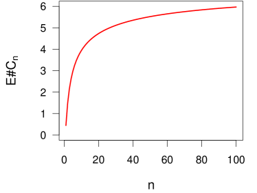
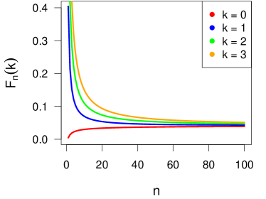
(a)	(b)

Figure 2. (a) $\mathbb{E}\#\mathcal{C}_{n}$ versus $n$, (b) $F_{n}(k)=a_{n}k+b_{n}$ versus $n$ for $k=0,1,2,3$, for $a_{n}=\frac{0.4}{n}$, $b_{n}=0.05(1-\frac{1}{\log(n+2)})$, with $L=100$.

For small $h$, we can obtain an expression for $\mathbb{E}I_{\varphi}[t,t+h]$ in terms of $\varphi$ and $\#\mathcal{C}_{N[0,t]+1}$, up to the first order, in the spirit of Theorem 4.1.

Theorem 4.6.

We have

$$\lim_{h\downarrow 0}\frac{\mathbb{E}I_{\varphi}[t,t+h]}{h}=\lambda(t)\mathbb{E}\varphi(\#\mathcal{C}_{N[0,t]+1}+1).$$

4.3. An uninteresting special case

A main feature of the model (1) is that the co-author sets $\mathcal{C}_{n}$ are dependent. We now look at a situation where they become independent. A fortiori, the correlation between $X_{k}[t,t+h]$ and $X_{k^{\prime}}[t,t+h]$ becomes second order in $h$, and $\mathbb{E}I_{\varphi}[s,t]$ becomes a constant.

Corollary 4.7.

If for all $n\geq 1$, $F_{n}(k)$ does not depend on $k$, i.e. $F_{n}(k)=p_{n}$ for some $p_{n}\in[0,1]$, for all $0\leq k\leq n-1$, then the random sets $\mathcal{C}_{n}$ are independent. Further, if $F_{n}(k)$ depends neither on $k$ nor on $n$, i.e. if for all $n\geq 1$, $F_{n}(k)=p$ for some $p\in[0,1]$, for all $0\leq k\leq n-1$, then

• $\lim_{h\downarrow 0}\frac{\mathrm{Cor}(X_{k+1}[t,t+h],X_{k^{\prime}+1}[t,t+h])}{h}=0$ for any $k\neq k^{\prime}\geq 0$.

• $\mathbb{E}I_{\varphi}[s,t]=\mathbb{E}\varphi(B+1)$, where $B\sim\mathrm{Binomial}(L,p)$.

4.4. Asymptotic properties of the estimators

We first show that the estimators given by (3), (4) and (5) are all almost-surely well-defined as $L\to\infty$.

Theorem 4.8.

We have the following:

• Fix $n\geq 1$ and $k\in\{0\}\cup[n]$. Then

  $$\mathbb{P}\bigg{(}\liminf_{L\to\infty}\sum_{i\in[L]}\mathbb{I}\{m_{n,i}=k\}>0\bigg{)}=1.$$

• Fix $n\geq 1$. Then

  $$\mathbb{P}\bigg{(}\liminf_{L\to\infty}\bigg{[}\frac{1}{L}\sum_{i\in[L]}m^{2}_{n,i}-\bigg{(}\frac{1}{L}\sum_{i\in[L]}m_{n,i}\bigg{)}^{2}\bigg{]}>0\bigg{)}=1.$$

Note that for fixed $n$, $\{m_{n,i}\}_{i\in[L]}$ are i.i.d. Let $p_{n,k}:=\mathbb{P}(m_{n,1}=k)$ for $k\in\{0\}\cup[n]$.

Theorem 4.9 (Consistency and asymptotic normality of $\widehat{F}_{n}(k)$).

Fix $n\geq 1$ and $k\in\{0\}\cup[n-1]$. Then, as $L\to\infty$,

$$\widehat{F}_{n}(k)\stackrel{{\scriptstyle p}}{{\to}}F_{n}(k)$$ (15)

and

$$\sqrt{L}\big{(}\widehat{F}_{n}(k)-F_{n}(k)\big{)}\stackrel{{\scriptstyle d}}{{\to}}N(0,\sigma^{2}),$$ (16)

where

$$\sigma^{2}=\frac{F_{n}(k)(1-F_{n}(k))}{p_{n-1,k}}.$$ (17)

Corollary 4.10 (Asymptotic confidence interval for ${F}_{n}(k)$).

Let

$$\widehat{\sigma}^{2}:=\frac{\widehat{F}_{n}(k)(1-\widehat{F}_{n}(k))}{\frac{1}{L}\sum_{i\in[L]}\mathbb{I}(m_{n-1,i}=k)}.$$ (18)

Then an $(1-q)\%$ asymptotic confidence interval for ${F}_{n}(k)$ is given by

$$\bigg{(}\widehat{F}_{n}(k)-\frac{\widehat{\sigma}}{\sqrt{L}}z_{q/2},\widehat{F}_{n}(k)+\frac{\widehat{\sigma}}{\sqrt{L}}z_{q/2}\bigg{)},$$

where $z_{q/2}$ is the $(1-q/2)$-th quantile of the standard normal distribution.

Theorem 4.11 (Consistency and asymptotic normality of $\widehat{a}_{n}$ and $\widehat{b}_{n}$).

Fix $n\geq 1$. Then, as $L\to\infty$,

$$\widehat{a}_{n}\stackrel{{\scriptstyle p}}{{\to}}a_{n},\quad\widehat{b}_{n}\stackrel{{\scriptstyle p}}{{\to}}b_{n}$$

and

$$\sqrt{L}\big{(}\widehat{a}_{n}-{a}_{n}\big{)}\stackrel{{\scriptstyle d}}{{\to}}N(0,\sigma_{a}^{2}),\quad\sqrt{L}\big{(}\widehat{b}_{n}-{b}_{n}\big{)}\stackrel{{\scriptstyle d}}{{\to}}N(0,\sigma_{b}^{2}),$$ (19)

for some $\sigma^{2}_{a},\sigma^{2}_{b}>0$.

Remark 4.12.

Explicit expressions for $\sigma_{a}^{2}$ and $\sigma_{b}^{2}$ are derived in the proof of Theorem 4.11. Unfortunately, these expressions are not very pleasant to look at!

Corollary 4.13 (Asymptotic confidence intervals for $\widehat{a}_{n}$ and $\widehat{b}_{n}$).

There exists consistent estimators $\widehat{\sigma}^{2}_{a}$ and $\widehat{\sigma}^{2}_{b}$ of $\sigma^{2}_{a}$ and $\sigma^{2}_{b}$, respectively. An $(1-q)\%$ asymptotic confidence intervals for $a_{n}$ is given by

$$\bigg{(}\widehat{a}_{n}-\frac{\widehat{\sigma}_{a}}{\sqrt{L}}z_{q/2},\widehat{a}_{n}+\frac{\widehat{\sigma}_{a}}{\sqrt{L}}z_{q/2}\bigg{)},$$

and an $(1-q)\%$ asymptotic confidence intervals for $b_{n}$ is given by

$$\bigg{(}\widehat{b}_{n}-\frac{\widehat{\sigma}_{b}}{\sqrt{L}}z_{q/2},\widehat{b}_{n}+\frac{\widehat{\sigma}_{b}}{\sqrt{L}}z_{q/2}\bigg{)},$$

where, $z_{q/2}$ is the $(1-q/2)$-th quantile of the standard normal distribution.

5. Simulation studies

In this section, we study the behaviour of the indices of collaboration for various choices of the intensity functional $\lambda(t)$ and co-authorship probability parameters $(F_{n}(k))_{n\geq 1,k\geq 0}$ through a series of simulation experiments.

We plot the dynamics of the three collaboration coefficients ($I_{\mathrm{CI}}$, $I_{\mathrm{DC}}$, and $I_{\mathrm{CC}}$) in several different settings. In each setting, we use $L=100$ authors and report the values of the indices per year (i.e. $t-s=1$ year), averaged over $10$ Monte Carlo runs. These experiments are all run on a laptop with 8GB of RAM and an Intel Core i3-6006U CPU.

5.1. Effect of $F_{n}(k)$.

In the first three settings (shown in Figures 3-5), we take $\lambda(t)$ to be constant, so that the effect of the collaboration probabilities $F_{n}(k),n\geq 1,k\geq 0$ can be understood cleanly.

In the simplest case, shown in Figure 3, we take $F_{n}(k),0\leq k\leq n-1,n\geq 1,$ to be constant free of both $n$ and $k$. Note that all the three collaboration coefficients are essentially constant. This is what was shown in Corollary 4.7.

In the setting of Figure 4, we set $F_{n}(k)$ to be a function of $k$ only. In this case, the model does take the effect of past collaboration into account and this highly influences the dynamics of the various indices as seen from Figure 4.

Finally, in the setting of Figure 5, we set $F_{n}(\cdot)$ to be a (non-decreasing) function of $n$ only. Although the model does not take past history of collaboration into account in this case, the probabilities of collaboration (i.e. $F_{n}(k)$ for $k\geq 1$) do increase over the course of writing papers. This explains the non-decreasing nature of the curves shown in Figure 5.

5.2. Effect of $\lambda(t)$

In the settings of Figures 6-11, we use non-constant $\lambda(t)$ and the same $F_{n}(k)$’s as in Section 5.1. We use a piecewise constant $\lambda(t)$ in Figures 6-8 and a piecewise linear one in Figures 9-11.

We find from these experiments that the co-authorship probability functions $F_{n}(k)$ have a much greater impact on the indices of collaboration than $\lambda(t)$. Also, the simulations in Figures 6 and 7 confirm part (ii) of Corollary 4.7.

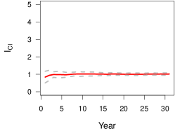
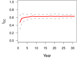
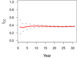
Figure 3. Different indices of collaboration for $\lambda(t)=0.5$ per month, and $F_{n}(k)=0.01$ for all $n\geq 1,k\geq 0$. In each subplot, the red line depicts yearly values of the corresponding index averaged over $10$ Monte Carlo runs. The dashed gray lines show $\pm 1$ standard errors.

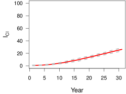
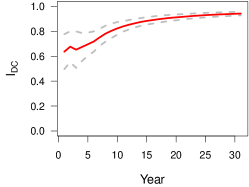
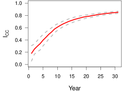
Figure 4. Different indices of collaboration for $\lambda(t)=0.5$ per month, and $F_{n}(k)=(0.05k+0.005)\wedge 1$ for all $n\geq 1$.

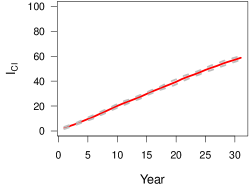
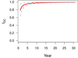
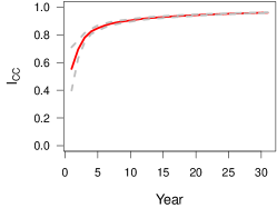
Figure 5. Different indices of collaboration for $\lambda(t)=0.5$ per month, and $F_{n}(k)=\frac{n}{180}\wedge 1$ for all $k\geq 0$.

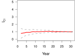
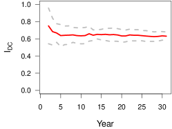
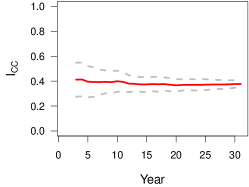
Figure 6. Different indices of collaboration for $\lambda(t)=\frac{1}{6}\mathbf{1}_{[0,100)}(t)+\frac{1}{3}\mathbf{1}_{[100,200)}(t)+\frac{1}{2}\mathbf{1}_{[200,\infty)}(t)$ per month, and $F_{n}(k)=0.01$ for all $n\geq 1,k\geq 0$.

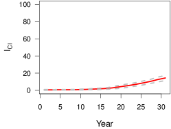
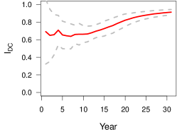
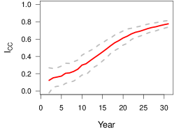
Figure 7. Different indices of collaboration for $\lambda(t)=\frac{1}{6}\mathbf{1}_{[0,100)}(t)+\frac{1}{3}\mathbf{1}_{[100,200)}(t)+\frac{1}{2}\mathbf{1}_{[200,\infty)}(t)$ per month, and $F_{n}(k)=(0.05k+0.005)\wedge 1$ for all $n\geq 1$.

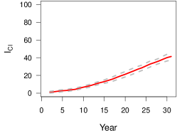
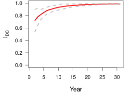
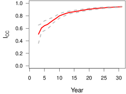
Figure 8. Different indices of collaboration for $\lambda(t)=\frac{1}{6}\mathbf{1}_{[0,100)}(t)+\frac{1}{3}\mathbf{1}_{[100,200)}(t)+\frac{1}{2}\mathbf{1}_{[200,\infty)}(t)$ per month, and $F_{n}(k)=\frac{n}{180}\wedge 1$ for all $k\geq 0$.

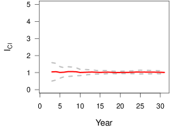
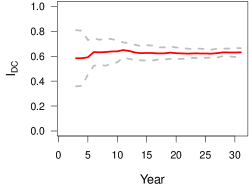
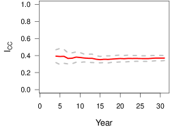
Figure 9. Different indices of collaboration for $\lambda(t)=\frac{t}{200}\mathbf{1}_{[0,100)}(t)+\frac{t}{400}\mathbf{1}_{[100,200)}(t)+\big{(}\frac{t}{720}\wedge 1\big{)}\mathbf{1}_{[200,\infty)}(t)$ per month, and $F_{n}(k)=0.01$ for all $n\geq 1,k\geq 0$.

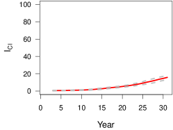
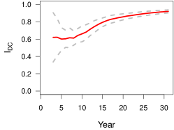
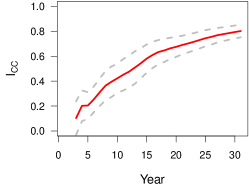
Figure 10. Different indices of collaboration for $\lambda(t)=\frac{t}{200}\mathbf{1}_{[0,100)}(t)+\frac{t}{400}\mathbf{1}_{[100,200)}(t)+\big{(}\frac{t}{720}\wedge 1\big{)}\mathbf{1}_{[200,\infty)}(t)$ per month, and $F_{n}(k)=(0.05k+0.005)\wedge 1$ for all $n\geq 1$.

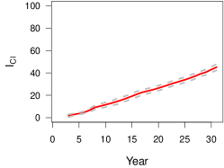
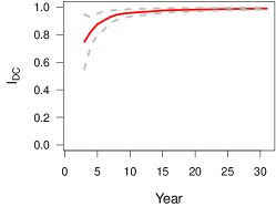
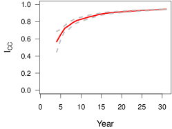
Figure 11. Different indices of collaboration for $\lambda(t)=\frac{t}{200}\mathbf{1}_{[0,100)}(t)+\frac{t}{400}\mathbf{1}_{[100,200)}(t)+\big{(}\frac{t}{720}\wedge\frac{1}{2}\big{)}\mathbf{1}_{[200,\infty)}(t)$ per month, and $F_{n}(k)=\frac{n}{180}\wedge 1$ for all $k\geq 0$.

6. Collaboration dynamics in Computer Science, Mathematics and Physics

We analyse the collaboration dynamics in several disciplines using data from the arXiv repository Clement et al. (2019). For each paper submitted to arXiv during the period 1991-2022, the dataset has three variables, namely, (i) id: unique identifier of the paper which also contains the time (month and year) of paper submission; (ii) categories: the discipline and/or the sub-discipline of the paper; (iii) authors: name of the authors of the paper. Therefore, the dataset has all the necessary information for computing the various indices of collaboration as a function of time.

Indices of collaboration. Since we are assuming a mean-field model, we consider all authors to be equivalent to any one individual author. The various indices of collaboration are computed by considering all papers written during a time-interval into account (c.f. the discussion in Section 3).

In Figure 12, we plot the three indices $I_{\mathrm{CI}}$, $I_{\mathrm{DC}}$ and $I_{\mathrm{CC}}$ per year. Further, we also consider the mean-field collaboration dynamics of the top $100$ most productive Computer Science (CS) authors (in terms of number of papers written) in order to understand the collaboration behaviour of extremely productive authors. In Figure 13, yearly indices computed based on the top 100 most productive authors are plotted. Notice that for a typical top author in CS, the indices indicate higher degree of collaboration than a typical author of the entire discipline. In fact, the $I_{\mathrm{CC}}$ index for them has reached almost 1 by 2020, i.e. they have mostly abandoned writing single-author papers!

We also construct similar plots for Mathematics and Physics — the various indices of collaboration are computed by taking either all papers written during a time-interval into account (Figures 14 and 16), or only the papers written by the top 100 most productive authors (Figures 15 and 17). As in the case of CS, we observe that for a typical top author, the indices indicate higher degree of collaboration than a typical author in both Mathematics and Physics. Also, the overall tendency of collaboration in Mathematics is much lower than that of CS and Physics.

No of co-authors per paper. In Figures 18-(a), 19-(a) and 20-(a), we plot the average number of co-authors in the $k$-th paper versus $k$, computed based on the top $100$ most productive authors in CS, Mathematics and Physics, respectively. The average number of co-authors in the $k$-th paper seems to increase as $k$ increases across all three disciplines. However, the behaviour of the rate of increment is markedly different — it gradually decreases in the case of CS, remains mostly a constant in the case of Mathematics and exhibits a rather interesting piecewise constant pattern in the case of Physics. The behaviour seen in the case of CS can qualitatively be explained via Lemma 4.4 (see, e.g., Figure 2-(a)). We also notice that for Physics, as $k$ increases, the rate of increase (as a function of $k$) in the number of co-authors in the $k$-th paper is much higher than the same for CS or Mathematics (likely due to the effect of very large collaborative projects in Physics).

Temporal behaviour of correlations. We choose $1000$ authors randomly from the set of all CS authors and plot in Figure 18-(b) the empirical correlation between $X_{1}[t,t+\delta]$ and $X_{k}[t,t+\delta]$ based on the observed values of $(X_{1}[t,t+\delta],X_{k}[t,t+\delta])$ for these authors for $k=2,3,4,5$ with $\delta=1$ year. Similar plots for Mathematics and Physics appear in Figures 19-(b) and 20-(b), respectively. These plots suggest the presence of non-trivial correlations.

Estimation of co-authorship probability parameters. Using the methodology described in Section 2.2, we estimate the co-authorship probability parameters $(F_{n}(k))_{n\geq 1}$ for $k=0,1,2,3$. Without loss of generality, let $[L_{1}]$ be the (random) set of authors who write a paper with $a_{0}$ at some point of time and let $[L_{2}]:=[L]\setminus[L_{1}]$. Then we may write

$$\widehat{F}_{n}(k)=\frac{\sum_{i\in[L_{1}]}\mathbb{I}(m_{n-1,i}=k)\mathbf{1}_{\mathcal{C}_{n}}(i)}{\sum_{i\in[L_{1}]}\mathbb{I}(m_{n-1,i}=k)+\sum_{i\in[L_{2}]}\mathbb{I}(m_{n-1,i}=k)}.$$

Note that

$$\sum_{i\in[L_{2}]}\mathbb{I}(m_{n-1,i}=k)=\begin{cases}L_{2}&\text{ if }k=0,\\ 0&\text{ if }k\geq 1.\end{cases}$$

While the terms $\sum_{i\in[L_{1}]}\mathbb{I}(m_{n-1,i}=k)\mathbf{1}_{\mathcal{C}_{n}}(i)$ and $\sum_{i\in[L_{1}]}\mathbb{I}(m_{n-1,i}=k)$ are easy to estimate, the value of $L_{2}$ is computationally expensive to estimate for a large time-series of collaboration data. For simplicity, we estimate $L_{2}$ by $M-\sum_{i\in[L_{1}]}\mathbb{I}(m_{n-1,i}=k)$, where $M$ is the maximum (over all months) of the monthly counts of productive authors (i.e. authors who have written a paper in that month).

We plot the estimated co-authorship probability parameters $(F_{n}(k))_{n\geq 1}$ for $k=0,1,2,3$ in Figures 18-(c), 19-(c) and 20-(c). Notice the qualitative similarity of these plots with Figure 2-(b), where we plot these parameters for an instance of the simple parametric sub-model (2).

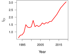
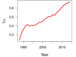
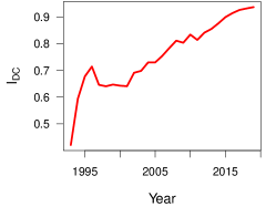
Figure 12. ArXiv data for CS: Yearly plot of $I_{\mathrm{CI}}$, $I_{\mathrm{DC}}$, and $I_{\mathrm{CC}}$ based on all authors.

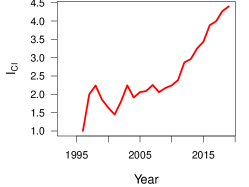
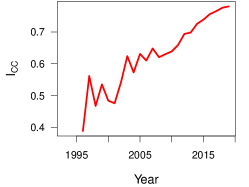
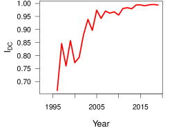
Figure 13. ArXiv data for CS: Yearly plot of $I_{\mathrm{CI}}$, $I_{\mathrm{DC}}$, and $I_{\mathrm{CC}}$ based on the top $100$ authors.

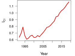
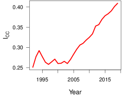
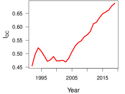
Figure 14. ArXiv data for Mathematics: Yearly plot of $I_{\mathrm{CI}}$, $I_{\mathrm{DC}}$, and $I_{\mathrm{CC}}$ based on all authors.

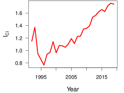
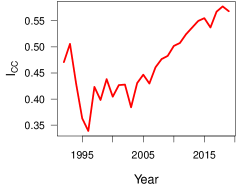
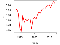
Figure 15. ArXiv data for Mathematics: Yearly plot of $I_{\mathrm{CI}}$, $I_{\mathrm{DC}}$, and $I_{\mathrm{CC}}$ based on the top $100$ authors.

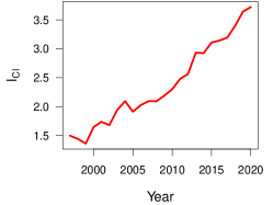
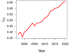
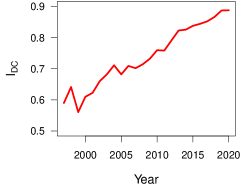
Figure 16. ArXiv data for Physics: Yearly plot of $I_{\mathrm{CI}}$, $I_{\mathrm{DC}}$, and $I_{\mathrm{CC}}$ based on all authors.

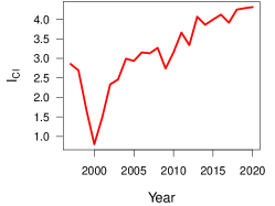
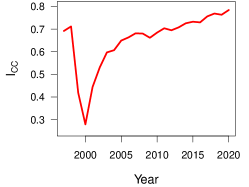
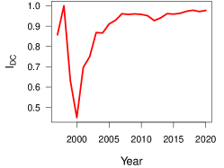
Figure 17. ArXiv data for Physics: Yearly plot of $I_{\mathrm{CI}}$, $I_{\mathrm{DC}}$, and $I_{\mathrm{CC}}$ based on the top $100$ authors.

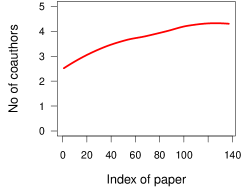
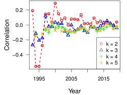
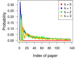
(a)	(b)	(c)

Figure 18. ArXiv data for CS: (a) Plot of the no of co-authors in the $k$-th paper of an author versus $k$ (based on the top 100 most productive authors); (b) plot of $\mathrm{Cor}(X_{1}[t,t+\delta],X_{k}[t,t+\delta])$, for $\delta=1$ year; (c) plot of $\widehat{F}_{n}(k)$ versus $n$.

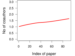
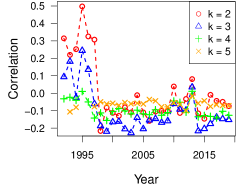
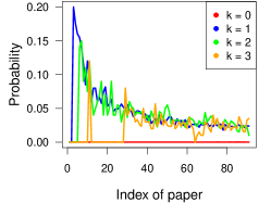
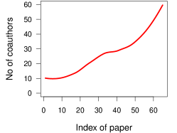
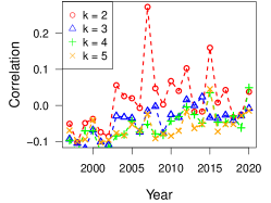
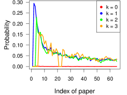
(a)	(b)	(c)

Figure 19. ArXiv data for Mathematics: (a) Plot of the no of co-authors in the $k$-th paper of an author versus $k$ (based on the top 100 most productive authors); (b) plot of $\mathrm{Cor}(X_{1}[t,t+\delta],X_{k}[t,t+\delta])$, for $\delta=1$ year; (c) plot of $\widehat{F}_{n}(k)$ versus $n$.

(a)	(b)	(c)

Figure 20. ArXiv data for Physics: (a) Plot of the no of co-authors in the $k$-th paper of an author versus $k$ (based on the top 100 most productive authors); (b) plot of $\mathrm{Cor}(X_{1}[t,t+\delta],X_{k}[t,t+\delta])$, for $\delta=1$ year; (c) plot of $\widehat{F}_{n}(k)$ versus $n$.

7. Conclusion

In this work, we introduce a novel mean-field dynamic model for academic collaboration, by combining a non-homogeneous Poisson process modeling paper-writing events and a mechanism of choosing co-authors depending on past collaboration history. We also develop methods for estimating the (infinite dimensional) parameters of the model. We derive analytical expressions for various indices of collaboration under the proposed model in terms of the model parameters. The proposed model is highly flexible in that it can explain a variety of empirically observed features found in real-world collaboration networks. For example, the behaviours of various indices of collaboration over time, or the effect that people tend to collaborate more with people they have already collaborated with in the past, but this effect seems to reverse as the number of joint collaborations increase over time.

Although the proposed model reflects many complexities of real-world collaboration networks, there are some limitations. For example, the mean-field nature of the model overlooks the fact that the intensity of producing research vary across authors. This can potentially be tackled by considering the collaboration dynamics of all authors simultaneously, allocating each a separate intensity functional. Also, in the proposed model, an author does not consider the relative impacts (measured in terms of the impact factor of the journal in which a work is published, or the number of times the work has been cited) of various existing research works while choosing future collaborators. Nor does she take into account how successful the potential collaborators are. We believe that the proposed model can be suitably tweaked to incorporate these effects and leave the exploration of such extensions to future work. Furthermore, the proposed framework can also be adopted to study evolution of interdisciplinary research collaboration by assigning each author a discipline or specific field of research based on their publication record. We will pursue this direction in a future work.

Funding

SSM is partially supported by an INSPIRE research grant (DST/INSPIRE/04/2018/002193) from the Department of Science and Technology, Government of India.

Appendix A Proofs of our main results

We begin with a technical lemma which will be used repeatedly later in various proofs.

Lemma A.1.

Let $N$ be an inhomogeneous Poisson process with intensity functional $\lambda(\cdot)$, whose event times are $E_{n},n\geq 1$. Let $U=N[0,t]$ and $\lambda_{t,h}=\int_{t}^{t+h}\lambda(u)\,du$. Then, for all $t,h>0$ satisfying $\lambda_{t,h}<1$ and any functions $g:\mathbb{N}\rightarrow[0,1]$ and $h:\mathbb{N}\times\mathbb{N}\rightarrow[0,1]$, the following inequalities hold:

$$\bigg{|}\sum_{n\geq 1}g(n)\mathbb{P}(E_{n}\in[t,t+h])-e^{-\lambda_{t,h}}\lambda_{t,h}\sum_{n\geq 1}g(n)\mathbb{P}(U=n-1)\bigg{|}\leq\lambda_{t,h}^{2}+\frac{\lambda_{t,h}^{2}}{1-\lambda_{t,h}};$$ (20)

$$\bigg{|}\sum_{\begin{subarray}{c}n_{1}\geq 1\\ n_{2}>n_{1}\end{subarray}}h(n_{1},n_{2})\mathbb{P}(E_{n_{1}},E_{n_{2}}\in[t,t+h])-e^{-\lambda_{t,h}}\frac{\lambda_{t,h}^{2}}{2}\sum_{n\geq 1}h(n,n+1)\mathbb{P}(U=n-1)\bigg{|}$$

$$\hskip 220.00034pt\leq\lambda_{t,h}^{3}+\frac{\lambda_{t,h}^{3}}{1-\lambda_{t,h}}+\frac{\lambda_{t,h}^{3}}{\big{(}1-\lambda_{t,h}\big{)}^{2}}.$$ (21)

Proof.

Let $\Lambda(t)=\int_{0}^{t}\lambda(u)\,du$ and $V=N[t,t+h]$. Note that $U$ and $V$ are independent, $U\sim\mathsf{Poisson}(\Lambda(t))$ and $V\sim\mathsf{Poisson}(\lambda_{t,h})$. Now if $W\sim\mathsf{Poisson}(\mu)$, then we have the estimate

$$\mathbb{P}(W\geq k)=e^{-\mu}\sum_{\ell\geq k}\frac{\mu^{\ell}}{\ell!}=e^{-\mu}\mu^{k}\sum_{\ell\geq k}\frac{\mu^{\ell-k}}{\ell!}\leq e^{-\mu}\mu^{k}\sum_{\ell\geq k}\frac{\mu^{\ell-k}}{(\ell-k)!}=\mu^{k}.$$ (22)

Proof of (20). We begin by noting that

$$\mathbb{P}(E_{n}\in[t,t+h]) =\mathbb{P}(U\leq n-1,U+V\geq n)=\sum_{k=0}^{n-1}\mathbb{P}(U=k)\mathbb{P}(V\geq n-k).$$

Now

$$\sum_{n\geq 1} g(n)\mathbb{P}(E_{n}\in[t,t+h])$$

$$=\sum_{n\geq 1}g(n)\sum_{k=0}^{n-1}\mathbb{P}(U=k)\mathbb{P}(V\geq n-k)$$

$$=\sum_{n\geq 1}g(n)\mathbb{P}(U=n-1)\mathbb{P}(V\geq 1)+\sum_{n\geq 2}g(n)\sum_{k=0}^{n-2}\mathbb{P}(U=k)\mathbb{P}(V\geq n-k).$$

Therefore

$$0\leq\sum_{n\geq 1}g(n) \mathbb{P}(E_{n}\in[t,t+h])-e^{-\lambda_{t,h}}\lambda_{t,h}\sum_{n\geq 1}g(n)\mathbb{P}(U=n-1)$$

$$=\sum_{n\geq 1}g(n)\mathbb{P}(U=n-1)\mathbb{P}(V\geq 2)+\sum_{n\geq 2}g(n)\sum_{k=0}^{n-2}\mathbb{P}(U=k)\mathbb{P}(V\geq n-k)$$

$$\leq\mathbb{P}(V\geq 2)\sum_{n\geq 1}\mathbb{P}(U=n-1)+\sum_{k\geq 0}\mathbb{P}(U=k)\sum_{n\geq k+2}\mathbb{P}(V\geq n-k)$$

$$\leq\lambda_{t,h}^{2}+\sum_{k\geq 0}\mathbb{P}(U=k)\sum_{\ell\geq 2}\lambda_{t,h}^{\ell}\quad(\text{using \eqref{eq:poi_tail_trivial}})$$

$$=\lambda_{t,h}^{2}+\frac{\lambda_{t,h}^{2}}{1-\lambda_{t,h}}.$$

Proof of (21). Note that for $n_{2}>n_{1}$,

$$\mathbb{P}(E_{n_{1}},E_{n_{2}}\in[t,t+h])=\mathbb{P}(U\leq n_{1}-1,U+V\geq n_{2})=\sum_{k=0}^{n_{1}-1}\mathbb{P}(U=k)\mathbb{P}(V\geq n_{2}-k).$$

Now

$$\sum_{\begin{subarray}{c}n_{1}\geq 1\\ n_{2}>n_{1}\end{subarray}} h(n_{1},n_{2})\mathbb{P}(E_{n_{1}},E_{n_{2}}\in[t,t+h])$$

$$=\sum_{n\geq 1}h(n,n+1)\mathbb{P}(E_{n},E_{n+1}\in[t,t+h])+\sum_{\begin{subarray}{c}n_{1}\geq 1\\ n_{2}>n_{1}+1\end{subarray}}h(n_{1},n_{2})\mathbb{P}(E_{n_{1}},E_{n_{2}}\in[t,t+h])$$

$$=\sum_{n\geq 1}h(n,n+1)\sum_{k=0}^{n-1}\mathbb{P}(U=k)\mathbb{P}(V\geq n+1-k)$$

$$\hskip 150.00023pt+\sum_{\begin{subarray}{c}n_{1}\geq 1\\ n_{2}>n_{1}+1\end{subarray}}h(n_{1},n_{2})\sum_{k=0}^{n_{1}-1}\mathbb{P}(U=k)\mathbb{P}(V\geq n_{2}-k)$$

$$=\sum_{n\geq 1}h(n,n+1)\mathbb{P}(U=n-1)\mathbb{P}(V\geq 2)+\sum_{n\geq 2}h(n,n+1)\sum_{k=0}^{n-2}\mathbb{P}(U=k)\mathbb{P}(V\geq n+1-k)$$

$$\hskip 150.00023pt+\sum_{\begin{subarray}{c}n_{1}\geq 1\\ n_{2}>n_{1}+1\end{subarray}}h(n_{1},n_{2})\sum_{k=0}^{n_{1}-1}\mathbb{P}(U=k)\mathbb{P}(V\geq n_{2}-k).$$

Therefore

$$0\leq \sum_{\begin{subarray}{c}n_{1}\geq 1\\ n_{2}>n_{1}\end{subarray}}h(n_{1},n_{2})\mathbb{P}(E_{n_{1}},E_{n_{2}}\in[t,t+h])-e^{-\lambda_{t,h}}\frac{\lambda_{t,h}^{2}}{2}\sum_{n\geq 1}h(n,n+1)\mathbb{P}(U=n-1)$$

$$=\sum_{n\geq 1}h(n,n+1)\mathbb{P}(U=n-1)\mathbb{P}(V\geq 3)+\sum_{n\geq 2}h(n,n+1)\sum_{k=0}^{n-2}\mathbb{P}(U=k)\mathbb{P}(V\geq n+1-k)$$

$$\hskip 150.00023pt+\sum_{\begin{subarray}{c}n_{1}\geq 1\\ n_{2}>n_{1}+1\end{subarray}}h(n_{1},n_{2})\sum_{k=0}^{n_{1}-1}\mathbb{P}(U=k)\mathbb{P}(V\geq n_{2}-k)$$

$$\leq\mathbb{P}(V\geq 3)\sum_{n\geq 1}\mathbb{P}(U=n-1)+\sum_{k\geq 0}\mathbb{P}(U=k)\sum_{n\geq k+2}\mathbb{P}(V\geq n+1-k)$$

$$\hskip 150.00023pt+\sum_{k\geq 0}\mathbb{P}(U=k)\sum_{n_{1}\geq k+1}\sum_{\ell\geq 2}\mathbb{P}(V\geq n_{1}+\ell-k)$$

$$\leq\lambda_{t,h}^{3}\sum_{n\geq 1}\mathbb{P}(U=n-1)+\sum_{k\geq 0}\mathbb{P}(U=k)\sum_{\ell\geq 3}\lambda_{t,h}^{\ell}$$

$$\hskip 150.00023pt+\sum_{k\geq 0}\mathbb{P}(U=k)\sum_{n_{1}\geq k+1}\sum_{\ell\geq 2}\lambda_{t,h}^{n_{1}+\ell-k}\quad(\text{using \eqref{eq:poi_tail_trivial}})$$

$$=\lambda_{t,h}^{3}+\frac{\lambda_{t,h}^{3}}{1-\lambda_{t,h}}+\sum_{k\geq 0}\mathbb{P}(U=k)\sum_{n_{1}\geq k+1}\frac{\lambda_{t,h}^{n_{1}+2-k}}{1-\lambda_{t,h}}$$

$$=\lambda_{t,h}^{3}+\frac{\lambda_{t,h}^{3}}{1-\lambda_{t,h}}+\frac{\lambda_{t,h}^{3}}{(1-\lambda_{t,h})^{2}}.$$

This completes the proof. ∎

We now use Lemma A.1 to estimate various moments of $X_{k}[t,t+h]$.

Lemma A.2.

We have

$$\mathbb{E}X_{k+1}[t,t+h] =e^{-\lambda_{t,h}}\lambda_{t,h}H_{t}(k)+R_{1}(t,h),$$ (23)

$$\mathbb{E}(X_{k+1}[t,t+h])^{2} =e^{-\lambda_{t,h}}(\lambda_{t,h}H_{t}(k)+\lambda_{t,h}^{2}G_{t}(k,k))+R_{2}(t,h),$$ (24)

$$\mathbb{E}(X_{k+1}[t,t+h]X_{k^{\prime}+1}[t,t+h]) =e^{-\lambda_{t,h}}\frac{\lambda_{t,h}^{2}}{2}(G_{t}(k,k^{\prime})+G_{t}(k^{\prime},k))+R_{3}(t,h),$$ (25)

where

$$|R_{1}(t,h)| \leq\lambda_{t,h}^{2}\bigg{(}1+\frac{1}{1-\lambda_{t,h}}\bigg{)},$$

$$|R_{2}(t,h)| \leq\lambda_{t,h}\bigg{(}1+\frac{1}{1-\lambda_{t,h}}\bigg{)}+2\lambda_{t,h}^{2}\bigg{(}1+\frac{1}{1-\lambda_{t,h}}+\frac{1}{(1-\lambda_{t,h})^{2}}\bigg{)},$$

$$|R_{3}(t,h)| \leq 2\lambda_{t,h}^{3}\bigg{(}1+\frac{1}{1-\lambda_{t,h}}+\frac{1}{(1-\lambda_{t,h})^{2}}\bigg{)}.$$

Proof.

We have

$$\mathbb{E}X_{k+1}[t,t+h] =\mathbb{E}\sum_{n\geq 1}\mathbb{I}(\#\mathcal{C}_{n}=k)\mathbf{1}_{[t,t+h]}(E_{n})$$

$$=\sum_{n\geq 1}\mathbb{P}(\#\mathcal{C}_{n}=k)\mathbb{P}(E_{n}\in[t,t+h])$$

$$=e^{-\lambda_{t,h}}\lambda_{t,h}\sum_{n\geq 1}\mathbb{P}(\#\mathcal{C}_{n}=k)\mathbb{P}(U=n-1)+R_{1}(t,h)$$

$$=e^{-\lambda_{t,h}}\lambda_{t,h}H_{t}(k)+R_{1}(t,h),$$

where $|R_{1}(t,h)|\leq\lambda_{t,h}^{2}(1+\frac{1}{1-\lambda_{t,h}})$ by (20).

On the other hand,

$$\mathbb{E}(X_{k+1}[t, t+h])^{2}$$

$$=\mathbb{E}\bigg{(}\sum_{n_{1}\geq 1}\mathbb{I}(\#\mathcal{C}_{n_{1}}=k)\mathbf{1}_{[t,t+h]}(E_{n_{1}})\bigg{)}\bigg{(}\sum_{n_{2}\geq 1}\mathbb{I}(\#\mathcal{C}_{n_{2}}=k)\mathbf{1}_{[t,t+h]}(E_{n_{2}})\bigg{)}$$

$$=\sum_{n_{1}}\mathbb{P}(\#\mathcal{C}_{n_{1}}=k)\mathbb{P}(E_{n_{1}}\in[t,t+h])$$

$$\qquad\qquad+2\sum_{\begin{subarray}{c}n_{1}\geq 1\\ n_{2}>n_{1}\end{subarray}}\mathbb{P}(\#\mathcal{C}_{n_{1}}=k,\#\mathcal{C}_{n_{2}}=k)\mathbb{P}(E_{n_{1}},E_{n_{2}}\in[t,t+h])$$

$$=e^{-\lambda_{t,h}}\lambda_{t,h}\sum_{n\geq 1}\mathbb{P}\bigg{(}\#\mathcal{C}_{n}=k\bigg{)}\mathbb{P}(U=n-1)$$

$$\qquad\qquad+2e^{-\lambda_{t,h}}\frac{\lambda_{t,h}^{2}}{2}\sum_{n\geq 1}\mathbb{P}(\#\mathcal{C}_{n}=k,\#\mathcal{C}_{n+1}=k^{\prime})\mathbb{P}(U=n-1)+R_{2}(t,h)$$

$$=e^{-\lambda_{t,h}}\bigg{(}\lambda_{t,h}H_{t}(k)+\frac{\lambda_{t,h}^{2}}{2}G_{t}(k,k)\bigg{)}+R_{2}(t,h),$$

where $|R_{2}(t,h)|\leq\lambda_{t,h}(1+\frac{1}{1-\lambda_{t,h}})+2\lambda_{t,h}^{3}(1+\frac{1}{1-\lambda_{t,h}}+\frac{1}{(1-\lambda_{t,h})^{2}})$ by (20) and (21).

Finally,

$$\mathbb{E}(X_{k+1}[t,t+h] X_{k^{\prime}+1}[t,t+h])$$

$$=\mathbb{E}\bigg{(}\sum_{n_{1}\geq 1}\mathbb{I}(\#\mathcal{C}_{n_{1}}=k)\mathbf{1}_{[t,t+h]}(E_{n_{1}})\bigg{)}\bigg{(}\sum_{n_{2}\geq 1}\mathbb{I}(\#\mathcal{C}_{n_{2}}=k^{\prime})\mathbf{1}_{[t,t+h]}(E_{n_{2}})\bigg{)}$$

$$=\sum_{\begin{subarray}{c}n_{1}\geq 1\\ n_{2}>n_{1}\end{subarray}}\mathbb{P}(\#\mathcal{C}_{n_{1}}=k,\#\mathcal{C}_{n_{2}}=k^{\prime})\mathbb{P}(E_{n_{1}},E_{n_{2}}\in[t,t+h])$$

$$\qquad\qquad+\sum_{\begin{subarray}{c}n_{2}\geq 1\\ n_{1}>n_{2}\end{subarray}}\mathbb{P}(\#\mathcal{C}_{n_{1}}=k,\#\mathcal{C}_{n_{2}}=k^{\prime})\mathbb{P}(E_{n_{1}},E_{n_{2}}\in[t,t+h])$$

$$=e^{-\lambda_{t,h}}\frac{\lambda_{t,h}^{2}}{2}\sum_{n\geq 1}\mathbb{P}(\#\mathcal{C}_{n}=k,\#\mathcal{C}_{n+1}=k^{\prime})\mathbb{P}(U=n-1)$$

$$\qquad\qquad+e^{-\lambda_{t,h}}\frac{\lambda_{t,h}^{2}}{2}\sum_{n\geq 1}\mathbb{P}(\#\mathcal{C}_{n+1}=k,\#\mathcal{C}_{n}=k^{\prime})\mathbb{P}(U=n-1)+R_{3}(t,h)$$

$$=e^{-\lambda_{t,h}}\frac{\lambda_{t,h}^{2}}{2}(G_{t}(k,k^{\prime})+G_{t}(k^{\prime},k))+R_{3}(t,h),$$

where $|R_{3}(t,h)|\leq 2\lambda_{t,h}^{3}(1+\frac{1}{1-\lambda_{t,h}}+\frac{1}{(1-\lambda_{t,h})^{2}})$ by (21). ∎

Proof of Theorem 4.1.

Follows from the estimates in Lemma A.2 and the fact that $\lim_{h\downarrow 0}\frac{\lambda_{t,h}}{h}=\lambda(t)$. ∎

Proof of Lemma 4.2.

Note that

$$I_{\varphi}[s,t] =\frac{\sum_{k\geq 1}\varphi(k)X_{k}[s,t]}{N[s,t]}$$

$$=\frac{\sum_{k\geq 1}\varphi(k)\sum_{n\geq 1}\mathbb{I}(\#\mathcal{C}_{n}=k-1)\mathbf{1}_{[s,t]}(E_{n})}{N[s,t]}$$

$$=\sum_{n\geq 1}\frac{\mathbf{1}_{[s,t]}(E_{n})}{N[s,t]}\sum_{k\geq 1}\varphi(k)\mathbb{I}(\#\mathcal{C}_{n}=k-1)$$

$$=\sum_{n\geq 1}\frac{\mathbf{1}_{[s,t]}(E_{n})}{N[s,t]}\varphi(\#\mathcal{C}_{n}+1).$$

The desired result now follows from the independence of $N$ and $\mathcal{C}_{n}$. ∎

Proof of Lemma 4.3.

Note that $\mathbf{1}_{[s,t]}(E_{n})=1$ if and only if $U\leq n-1$ and $U+V\geq n$. ∎

Proof of Corollary 4.7.

That $\mathcal{C}_{n}$’s are independent when $F_{n}(k)=p_{n}$ for all $0\leq k\leq n-1$ is clear. In fact, in this case $\#\mathcal{C}_{n}\sim\mathrm{Binomial}(L,p_{n})$.

If $F_{n}(k)=p$ for all $0\leq k\leq n-1,n\geq 1$, then $\#C_{n}\overset{d}{=}B\sim\mathrm{Binomial}(L,p)$. Therefore, using the fact that the sets $\mathcal{C}_{n}$, $n\geq 1$, are independent across themselves and also of $U=N[0,t]$, we have

$$G_{t}(k,k^{\prime}) =\mathbb{P}(\#\mathcal{C}_{U+1}=k,\#\mathcal{C}_{U+2}=k^{\prime})$$

$$=\mathbb{E}_{U}\mathbb{P}(\#\mathcal{C}_{U+1}=k,\#\mathcal{C}_{U+2}=k^{\prime}\mid U)$$

$$=\mathbb{E}_{U}\mathbb{P}(\#\mathcal{C}_{U+1}=k)\mathbb{P}(\#\mathcal{C}_{U+2}=k^{\prime})$$

$$=\mathbb{P}(B=k)\mathbb{P}(B=k^{\prime}).$$

Similarly, $G_{t}(k^{\prime},k)=\mathbb{P}(B=k)\mathbb{P}(B=k^{\prime})$, and $H_{t}(k)=\mathbb{P}(B=k)$. Part (i) now follows Theorem 4.1.

Since $\mathbb{E}\varphi(\#\mathcal{C}_{n}+1)=\mathbb{E}\varphi(B+1)$, we have from Lemma 4.2 that

$$\mathbb{E}I_{\varphi}[t,t+h] =\sum_{n\geq 1}\mathbb{E}\bigg{[}\frac{\mathbf{1}_{[t,t+h]}(E_{n})}{N[t,t+h]}\bigg{]}\mathbb{E}\varphi(\#\mathcal{C}_{n}+1)$$

$$=\mathbb{E}\varphi(B+1)\sum_{n\geq 1}\mathbb{E}\bigg{[}\frac{\mathbf{1}_{[t,t+h]}(E_{n})}{N[t,t+h]}\bigg{]}$$

$$=\mathbb{E}\varphi(B+1)\mathbb{E}\sum_{n\geq 1}\frac{\mathbf{1}_{[t,t+h]}(E_{n})}{N[t,t+h]}$$

$$=\mathbb{E}\varphi(B+1).$$

This completes the proof of part (ii). ∎

Proof of Lemma 4.4.

We have

$$\mathbb{E}[\#\mathcal{C}_{n}\mid\mathcal{C}_{1},\ldots,\mathcal{C}_{n-1}] =\sum_{i=1}^{L}(a_{n}m_{n-1,i}+b_{n})$$

$$=a_{n}\sum_{i=1}^{L}m_{n-1,i}+Lb_{n}$$

$$=a_{n}\sum_{i=1}^{L}\sum_{\ell=1}^{n-1}\mathbf{1}_{\mathcal{C}_{\ell}}(i)+Lb_{n}$$

$$=a_{n}\sum_{\ell=1}^{n-1}\sum_{i=1}^{L}\mathbf{1}_{\mathcal{C}_{\ell}}(i)+Lb_{n}$$

$$=a_{n}\sum_{\ell=1}^{n-1}\#\mathcal{C}_{\ell}+Lb_{n}.$$

Now the desired result follows by taking expectation with respect to $\mathcal{C}_{1},\ldots,\mathcal{C}_{n-1}$. ∎

Proof of Lemma 4.5.

Write $A_{n}=\mathbb{E}\#\mathcal{C}_{n}$. Define $S_{n}=\sum_{\ell=1}^{n}A_{\ell}$, with $S_{0}:=0$. Then we have for any $n\geq 1$,

$$A_{n}=a_{n}S_{n-1}+Lb_{n}$$

and

$$S_{n}=S_{n-1}+A_{n}=(1+a_{n})S_{n-1}+Lb_{n}.$$

By iterating backwards, it is easy to see that

$$S_{n} =(1+a_{n})S_{n-1}+Lb_{n}$$

$$=(1+a_{n})(1+a_{n-1})S_{n-2}+L(b_{n}+b_{n-1}(1+a_{n}))$$

$$=(1+a_{n})(1+a_{n-1})(1+a_{n-2})S_{n-3}+L(b_{n}+b_{n-1}(1+a_{n})+b_{n-2}(1+a_{n-1})(1+a_{n}))$$

$$\,\,\,\vdots$$

$$=\prod_{j=2}^{n}(1+a_{j})S_{0}+L\bigg{(}b_{n}+\sum_{j=1}^{n-1}b_{j}\prod_{\ell=j+1}^{n}(1+a_{\ell})\bigg{)}$$

$$=L\bigg{(}b_{n}+\sum_{j=1}^{n-1}b_{j}\prod_{\ell=j+1}^{n}(1+a_{\ell})\bigg{)}.$$

Thus

$$A_{n} =S_{n}-S_{n-1}$$

$$=L\bigg{(}b_{n}+\sum_{j=1}^{n-1}b_{j}\prod_{\ell=j+1}^{n}(1+a_{\ell})-b_{n-1}-\sum_{j=1}^{n-2}b_{j}\prod_{\ell=j+1}^{n-1}(1+a_{\ell})\bigg{)}$$

$$=L\bigg{(}b_{n}+b_{n-1}a_{n}+\sum_{j=1}^{n-2}b_{j}a_{n}\prod_{\ell=j+1}^{n-1}(1+a_{\ell})\bigg{)}.$$

This completes the proof. ∎

Proof of Theorem 4.6.

Recall that

$$\mathbb{E}I_{\varphi}[t,t+h]=\sum_{n\geq 1}\mathbb{E}\bigg{[}\frac{\mathbf{1}_{[t,t+h]}(E_{n})}{N[t,t+h]}\bigg{]}\mathbb{E}\varphi(\#\mathcal{C}_{n}+1).$$

Since

$$\mathbb{E}\bigg{[}\frac{\mathbf{1}_{[t,t+h]}(E_{n})}{N[t,t+h]}\bigg{]}=\sum_{k=0}^{n-1}\mathbb{P}(U=k)\mathbb{E}\bigg{[}\frac{\mathbb{I}(V\geq n-k)}{V}\bigg{]}\geq\mathbb{P}(U=n-1)\mathbb{P}(V=1),$$

we have

$$\mathbb{E}I_{\varphi}[t,t+h] \geq\sum_{n\geq 1}\mathbb{P}(U=n-1)\mathbb{P}(V=1)\mathbb{E}\varphi(\#\mathcal{C}_{n}+1)$$

$$=\mathbb{P}(V=1)\sum_{n\geq 1}\mathbb{P}(U=n-1)\mathbb{E}\varphi(\#\mathcal{C}_{n}+1)$$

$$=e^{-\lambda_{t,h}}\lambda_{t,h}\mathbb{E}\varphi(\#\mathcal{C}_{U+1}+1).$$

On the other hand, since $\mathbb{E}\big{[}\frac{\mathbf{1}_{[t,t+h]}(E_{n})}{N[t,t+h]}\big{]}\leq\mathbb{P}(E_{n}\in[t,t+h])$, we have

$$\mathbb{E}I_{\varphi}[t,t+h] \leq\sum_{n\geq 1}\mathbb{E}\varphi(\#\mathcal{C}_{n}+1)\mathbb{P}(E_{n}\in[t,t+h])$$

$$=\varphi(L+1)\sum_{n\geq 1}\frac{\mathbb{E}\varphi(\#\mathcal{C}_{n}+1)}{\varphi(L+1)}\mathbb{P}(E_{n}\in[t,t+h])$$

$$=\varphi(L+1)\bigg{[}e^{-\lambda_{t,h}}\lambda_{t,h}\sum_{n\geq 1}\frac{\mathbb{E}\varphi(\#\mathcal{C}_{n}+1)}{\varphi(L+1)}\mathbb{P}(U=n-1)+R_{4}(t,h)\bigg{]}$$

$$=e^{-\lambda_{t,h}}\lambda_{t,h}\sum_{n\geq 1}\mathbb{E}\varphi(\#\mathcal{C}_{n}+1)\mathbb{P}(U=n-1)+\varphi(L+1)R_{4}(t,h)$$

$$=e^{-\lambda_{t,h}}\lambda_{t,h}\mathbb{E}\varphi(\#\mathcal{C}_{U+1}+1)+\varphi(L+1)R_{4}(t,h),$$

where $|R_{4}(t,h)|\leq\lambda_{t,h}^{2}(1+\frac{1}{1-\lambda_{t,h}})$.

We conclude that

$$|\mathbb{E}I_{\varphi}[t,t+h]-e^{-\lambda_{t,h}}\lambda_{t,h}\mathbb{E}\varphi(\#\mathcal{C}_{U+1}+1)|\leq\varphi(L+1)R_{4}(t,h).$$

The desired result now follows from the above estimate. ∎

Let $\mu_{n,r}$ be the $r$-th moment of $m_{n,1}$, given by

$$\mu_{n,r}:=\sum_{k=1}^{n}k^{r}p_{n,k}.$$

Proof of Theorem 4.8.

(a) Let us use the convention that for $n\geq 0$, $F_{n}(-1)=0,p_{0,0}=p_{n,n+1}=0$. Note that $p_{1,0}=1-F_{1}(0)>0$, and for $k\in[n]$, we have

$$p_{n,k} =\mathbb{P}(m_{n,1}=k)$$

$$=\mathbb{P}(m_{n,1}=k,m_{n-1,1}=k-1)+\mathbb{P}(m_{n,1}=k,m_{n-1,1}=k)$$

$$=\mathbb{P}(\mathbf{1}_{C_{n}}(1)=1\mid m_{n-1,1}=k-1)\mathbb{P}(m_{n-1,1}=k-1)$$

$$\qquad\qquad\qquad+\mathbb{P}(\mathbf{1}_{C_{n}}(1)=0\mid m_{n-1,1}=k)\mathbb{P}(m_{n-1,1}=k)$$

$$=F_{n}(k-1)p_{n-1,k-1}+(1-F_{n}(k))p_{n-1,k}.$$

By induction, we get that $p_{n,k}>0$ for all $n\geq 1$, $k=0,1,\ldots,n$. By the strong law of large numbers, as $L\to\infty$, we have that

$$\frac{1}{L}\sum_{i\in[L]}\mathbb{I}\{m_{n,i}=k\}\xrightarrow{\mathrm{a.s.}}p_{n,k}>0.$$ (26)

This completes the proof.

(b) Fix $n$. As $p_{n,k}>0$ for $k\in[n]$, we have $\mathrm{Var}(m_{n,1}):=\mu_{n,2}-\mu^{2}_{n,1}>0$. By the strong law of large numbers, as $L\to\infty$, we have that

$$\frac{1}{L}\sum_{i\in[L]}m^{2}_{n,i}\xrightarrow{\mathrm{a.s.}}\mu_{n,2},\quad\frac{1}{L}\sum_{i\in[L]}m_{n,i}\xrightarrow{\mathrm{a.s.}}\mu_{n,1}.$$

Therefore, as $L\to\infty$,

$$\frac{1}{L}\sum_{i\in[L]}m^{2}_{n,i}-\bigg{(}\frac{1}{L}\sum_{i\in[L]}m_{n,i}\bigg{)}^{2}\xrightarrow{\mathrm{a.s.}}\mu_{n,2}-\mu^{2}_{n,1}>0.$$

This completes the proof. ∎

Proof of Theorem 4.9.

Define the random variables

$$X_{i}=\mathbb{I}(m_{n-1,i}=k)\mathbf{1}_{\mathcal{C}_{n}}(i),\quad Y_{i}=\mathbb{I}(m_{n-1,i}=k),\quad i\in[L].$$

so that $X_{i}\stackrel{{\scriptstyle\mathrm{i.i.d.}}}{{\sim}}X_{1},Y_{i}\stackrel{{\scriptstyle\mathrm{i.i.d.}}}{{\sim}}Y_{1}$. Also, $X_{1},Y_{1}$ are Bernoulli random variables with

$$\mathbb{P}(Y_{1}=1)=\mathbb{P}(m_{n-1,1}=k)=p_{n-1,k}$$

and

$$\mathbb{P}(X_{1}=1) =\mathbb{P}(X_{1}=1,Y_{1}=1)$$

$$=\mathbb{P}(m_{n-1,1}=k,\mathbf{1}_{\mathcal{C}_{n}}(1)=1)$$

$$=\mathbb{P}(\mathbf{1}_{\mathcal{C}_{n}}(1)=1\mid m_{n-1,1}=k)\mathbb{P}(m_{n-1,1}=k)$$

$$=F_{n}(k)p_{n-1,k}.$$

Let

$$\mu_{x} :=\mathbb{E}(X_{1})=F_{n}(k)p_{n-1,k},$$

$$\mu_{y} :=\mathbb{E}(Y_{1})=p_{n-1,k},$$

$$\sigma_{x}^{2} :=\mathrm{Var}(X_{1})=F_{n}(k)p_{n-1,k}(1-F_{n}(k)p_{n-1,k}),$$

$$\sigma_{y}^{2} :=\mathrm{Var}(Y_{1})=p_{n-1,k}(1-p_{n-1,k}),$$

$$\rho\sigma_{x}\sigma_{y} :=\mathrm{Cov}(X_{1},Y_{1})=F_{n}(k)p_{n-1,k}-F_{n}(k)p^{2}_{n-1,k}.$$

Using Lemma B.1, we immediately get that

$$\widehat{F}_{n}(k)=\frac{\sum_{i\in[L]}\mathbb{I}(m_{n-1,i}=k)\mathbf{1}_{\mathcal{C}_{n}}(i)}{\sum_{i\in[L]}\mathbb{I}(m_{n-1,i}=k)}\xrightarrow{p}\frac{F_{n}(k)p_{n-1,k}}{p_{n-1,k}}=F_{n}(k)$$

and

$$\sqrt{L}\bigg{(}\widehat{F}_{n}(k)-F_{n}(k)\bigg{)}=\sqrt{L}\bigg{(}\frac{\sum_{i\in[L]}\mathbb{I}(m_{n-1,i}=k)\mathbf{1}_{\mathcal{C}_{n}}(i)}{\sum_{i\in[L]}\mathbb{I}(m_{n-1,i}=k)}-\frac{F_{n}(k)p_{n-1,k}}{p_{n-1,k}}\bigg{)}$$

converges in distribution to a normal random variable with mean $0$ and variance

$$\frac{p^{3}_{n-1,k}F_{n}(k)(1-F_{n}(k)p_{n-1,k})+F^{2}_{n}(k)p^{3}_{n-1,k}(1-p_{n-1,k})-2F^{2}_{n}(k)p^{3}_{n-1,k}(1-p_{n-1,k})}{p^{4}_{n-1,k}}$$

$$=\frac{F_{n}(k)(1-F_{n}(k)p_{n-1,k})+F^{2}_{n}(k)(1-p_{n-1,k})-2F^{2}_{n}(k)(1-p_{n-1,k})}{p_{n-1,k}}$$

$$=\frac{F_{n}(k)(1-F_{n}(k))}{p_{n-1,k}}.$$

This completes the proof. ∎

Proof of Corollary 4.10.

From (26), (15), (17) and (18), we get that

$$\widehat{\sigma}^{2}\xrightarrow{p}{\sigma}^{2}.$$ (27)

Then (16), (27) and Slutsky’s theorem implies that

$$\frac{\sqrt{L}\big{(}\widehat{F}_{n}(k)-F_{n}(k)\big{)}}{\widehat{\sigma}}\xrightarrow{d}N(0,1).$$

In other words,

$$1-q =\lim_{L\to\infty}\mathbb{P}\bigg{(}-z_{q/2}\leq\frac{\sqrt{L}\big{(}\widehat{F}_{n}(k)-F_{n}(k)\big{)}}{\widehat{\sigma}}\leq z_{q/2}\bigg{)}$$

$$=\lim_{L\to\infty}\mathbb{P}\bigg{(}{F}_{n}(k)\in\bigg{(}\widehat{F}_{n}(k)-\frac{\widehat{\sigma}}{\sqrt{L}}z_{q/2},\widehat{F}_{n}(k)+\frac{\widehat{\sigma}}{\sqrt{L}}z_{q/2}\bigg{)}\bigg{)}.$$

This completes the proof. ∎

Proof of Theorem 4.11.

Define the random variables

$$X_{i}:=\mathbf{1}_{\mathcal{C}_{n}}(i),\quad Y_{i}:=m_{n-1,i},\quad i\in[L]$$

so that $X_{i}\stackrel{{\scriptstyle\mathrm{i.i.d.}}}{{\sim}}X_{1},Y_{i}\stackrel{{\scriptstyle\mathrm{i.i.d.}}}{{\sim}}Y_{1}$. Then $X_{1}$ is a Bernoulli random variable and $Y_{1}$ is a discrete random variable taking values in $\{0\}\cup[n-1]$ with

$$\mathbb{P}(Y_{1}=k)=\mathbb{P}(m_{n-1,1}=k)=p_{n-1,k}.$$

For $\lambda>0$, let

$$s_{0,b}:=\mathbb{E}(Y_{1}^{\lambda})=\mu_{n-1,\lambda},$$

and for $\gamma>0,\lambda\geq 0$, let

$$s_{\gamma,\lambda}:=\mathbb{E}(X_{1}^{\gamma}Y_{1}^{\lambda}) =\sum_{k=1}^{n-1}k^{\lambda}\mathbb{P}(X_{1}=1,Y_{1}=k)$$

$$=\sum_{k=1}^{n-1}k^{\lambda}\mathbb{P}(\mathbf{1}_{\mathcal{C}_{n}}(1)=1\mid m_{n-1,1}=k)\mathbb{P}(m_{n-1,1}=k)$$

$$=\sum_{k=1}^{n-1}k^{\lambda}F_{n}(k)p_{n-1,k}$$

$$=a_{n}\sum_{k=1}^{n-1}k^{\lambda+1}p_{n-1,k}+b_{n}\sum_{k=1}^{n-1}k^{\lambda}p_{n-1,k}$$

$$=a_{n}\mu_{n-1,\lambda+1}+b_{n}\mu_{n-1,\lambda}.$$

Therefore

$$\Sigma=((\sigma_{ij})) :=\mathrm{Cov}(X_{1},Y_{1},Y_{1}^{2},X_{1}Y_{1})$$

$$=\begin{bmatrix}s_{1,0}-s^{2}_{1,0}&s_{1,1}-s_{1,0}s_{0,1}&s_{1,2}-s_{1,0}s_{0,2}&s_{2,1}-s_{1,0}s_{1,1}\\ s_{1,1}-s_{1,0}s_{0,1}&s_{0,2}-s^{2}_{0,1}&s_{0,3}-s_{0,1}s_{0,2}&s_{1,2}-s_{1,0}s_{1,1}\\ s_{1,2}-s_{1,0}s_{0,2}&s_{0,3}-s_{0,1}s_{0,2}&s_{0,4}-s_{0,2}^{2}&s_{1,3}-s_{0,2}s_{1,1}\\ s_{2,1}-s_{1,0}s_{1,1}&s_{1,2}-s_{1,0}s_{1,1}&s_{1,3}-s_{0,2}s_{1,1}&s_{2,2}-s^{2}_{1,1}\end{bmatrix}$$

and

$$\mu_{x} :=\mathbb{E}(X_{1})=a_{n}\mu_{n-1,1}+b_{n},$$

$$\mu_{y} :=\mathbb{E}(Y_{1})=\mu_{n-1,1},$$

$$\sigma_{x}^{2} :=\sigma_{11}=(a_{n}\mu_{n-1,1}+b_{n})(1-a_{n}\mu_{n-1,1}-b_{n}),$$

$$\sigma_{y}^{2} :=\sigma_{22}=\mu_{n-1,2}-\mu_{n-1,1}^{2},$$

$$\beta :=\frac{\rho\sigma_{x}\sigma_{y}}{\sigma_{y}^{2}}=\frac{\sigma_{12}}{\sigma_{22}}=\frac{a_{n}\mu_{n-1,2}+b_{n}\mu_{n-1,1}-(a_{n}\mu_{n-1,1}+b_{n})\mu_{n-1,1}}{\mu_{n-1,2}-\mu_{n-1,1}^{2}}=a_{n},$$

$$\alpha :=\mu_{x}-\beta\mu_{y}=a_{n}\mu_{n-1,1}+b_{n}-a_{n}\mu_{n-1,1}=b_{n}.$$

Thus $\widehat{\beta}=\widehat{a}_{n}$, $\widehat{\alpha}=\widehat{b}_{n}$. Then, parts (a) and (b) of Lemma B.2 immediately imply that

$$\widehat{a}_{n}\xrightarrow{p}a_{n},\quad\widehat{b}_{n}\xrightarrow{p}b_{n}$$

and

$$\sqrt{L}(\widehat{a}_{n}-a_{n})\xrightarrow{d}N(0,\sigma_{a}^{2}),\quad\sqrt{L}(\widehat{b}_{n}-b_{n})\xrightarrow{d}N(0,\sigma_{b}^{2}),$$

where

$$\sigma_{a}^{2} =\frac{\mu_{y}^{2}\sigma_{11}}{\sigma_{y}^{4}}+\frac{2\alpha\mu_{y}\sigma_{12}}{\sigma_{y}^{2}}+\frac{2\beta\mu_{y}\sigma_{13}}{\sigma_{y}^{4}}-\frac{2\mu_{y}\sigma_{14}}{\sigma_{y}^{4}}+\frac{\alpha^{2}\sigma_{22}}{\sigma_{y}^{4}}$$

$$\qquad\qquad+\frac{2\alpha\beta\sigma_{23}}{\sigma_{y}^{4}}-\frac{2\alpha\sigma_{24}}{\sigma_{y}^{4}}+\frac{\beta^{2}\sigma_{33}}{\sigma_{y}^{4}}-\frac{2\beta\sigma_{34}}{\sigma_{y}^{4}}+\frac{\sigma_{44}}{\sigma_{y}^{4}}$$

and

$$\sigma_{b}^{2} =\bigg{(}1+\frac{\mu_{y}^{2}}{\sigma_{y}^{2}}\bigg{)}^{2}\sigma_{11}-2\bigg{(}1+\frac{\mu_{y}^{2}}{\sigma_{y}^{2}}\bigg{)}\bigg{(}\frac{\beta\sigma_{y}^{2}+2\beta\mu_{y}^{2}-\mu_{x}\mu_{y}}{\sigma_{y}^{2}}\bigg{)}\sigma_{12}+2\bigg{(}1+\frac{\mu_{y}^{2}}{\sigma_{y}^{2}}\bigg{)}\frac{\beta\mu_{y}\sigma_{13}}{\sigma_{y}^{2}}$$

$$\qquad-2\bigg{(}1+\frac{\mu_{y}^{2}}{\sigma_{y}^{2}}\bigg{)}\frac{\mu_{y}\sigma_{14}}{\sigma_{y}^{2}}+\bigg{(}\frac{\beta\sigma^{2}_{y}+2\beta\mu_{y}^{2}-\mu_{x}\mu_{y}}{\sigma_{y}^{2}}\bigg{)}^{2}\sigma_{22}$$

$$\qquad-2\bigg{(}\frac{\beta\sigma_{y}^{2}+2\beta\mu_{y}^{2}-\mu_{x}\mu_{y}}{\sigma_{y}^{2}}\bigg{)}\frac{\beta\mu_{y}\sigma_{23}}{\sigma_{y}^{2}}$$

$$\qquad+2\bigg{(}\frac{\beta\sigma_{y}^{2}+2\beta\mu_{y}^{2}-\mu_{x}\mu_{y}}{\sigma_{y}^{2}}\bigg{)}\frac{\mu_{y}\sigma_{24}}{\sigma_{y}^{2}}+\frac{\beta^{2}\mu_{y}^{2}\sigma_{33}}{\sigma_{y}^{4}}-\frac{2\beta\mu_{y}^{2}\sigma_{34}}{\sigma_{y}^{4}}+\frac{\mu_{y}^{2}\sigma_{44}}{\sigma_{y}^{4}}.$$

This completes the proof. ∎

Proof of Corollary 4.13.

Part (c) of Lemma B.2 implies the existence of consistent estimators $\widehat{\sigma}^{2}_{a}$ and $\widehat{\sigma}^{2}_{b}$ of $\sigma^{2}_{a}$ and $\sigma^{2}_{b}$, respectively. Then (19) and Slutsky’s theorem gives that

$$\frac{\sqrt{L}(\widehat{a}_{n}-a_{n})}{\widehat{\sigma}_{a}}\xrightarrow{d}N(0,1)$$

and

$$\frac{\sqrt{L}(\widehat{b}_{n}-b_{n})}{\widehat{\sigma}_{b}}\xrightarrow{d}N(0,1).$$

In other words,

$$1-q =\lim_{L\to\infty}\mathbb{P}\bigg{(}-z_{q/2}\leq\frac{\sqrt{L}(\widehat{a}_{n}-a_{n})}{\widehat{\sigma}_{a}}\leq z_{q/2}\bigg{)}$$

$$=\lim_{L\to\infty}\mathbb{P}\bigg{(}a_{n}\in\bigg{(}\widehat{a}_{n}-\frac{\widehat{\sigma}_{a}}{\sqrt{L}}z_{q/2},\widehat{a}_{n}+\frac{\widehat{\sigma}_{a}}{\sqrt{L}}z_{q/2}\bigg{)}\bigg{)}$$

and

$$1-q =\lim_{L\to\infty}\mathbb{P}\bigg{(}-z_{q/2}\leq\frac{\sqrt{L}(\widehat{b}_{n}-b_{n})}{\widehat{\sigma}_{b}}\leq z_{q/2}\bigg{)}$$

$$=\lim_{L\to\infty}\mathbb{P}\bigg{(}b_{n}\in\bigg{(}\widehat{b}_{n}-\frac{\widehat{\sigma}_{b}}{\sqrt{L}}z_{q/2},\widehat{b}_{n}+\frac{\widehat{\sigma}_{b}}{\sqrt{L}}z_{q/2}\bigg{)}\bigg{)}.$$

This completes the proof. ∎

Appendix B Technical lemmas

Lemma B.1.

Suppose that $(X_{i},Y_{i}),i\geq 1,$ are i.i.d. nonnegative bivariate random vectors with $\mathbb{E}(X_{1})=\mu_{x}$, $\mathbb{E}(Y_{1})=\mu_{y}\neq 0$, $\mathrm{Var}(X_{1})=\sigma_{x}^{2}$, $\mathrm{Var}(Y_{1})=\sigma_{y}^{2}$ and $\mathrm{Cor}(X_{1},Y_{1})=\rho$. Then

$$\frac{\sum_{i=1}^{n}X_{i}}{\sum_{i=1}^{n}Y_{i}}\xrightarrow{p}\frac{\mu_{x}}{\mu_{y}}\quad\text{and}\quad\sqrt{n}\bigg{(}\frac{\sum_{i=1}^{n}X_{i}}{\sum_{i=1}^{n}Y_{i}}-\frac{\mu_{x}}{\mu_{y}}\bigg{)}\xrightarrow{d}N(0,\sigma_{0}^{2}),$$

where

$$\sigma_{0}^{2}=\frac{\mu_{y}^{2}\sigma_{x}^{2}+\mu_{x}^{2}\sigma_{y}^{2}-2\rho\mu_{x}\mu_{y}\sigma_{x}\sigma_{y}}{\mu_{y}^{4}}.$$

Proof.

By the weak law of large numbers,

$$(\bar{X}_{n},\bar{Y}_{n}):=\bigg{(}\frac{1}{n}\sum_{i=1}^{n}X_{i},\frac{1}{n}\sum_{i=1}^{n}Y_{i}\bigg{)}\xrightarrow{p}(\mu_{x},\mu_{y}).$$

Applying the continuous mapping theorem with the map

$$(x,y)\mapsto\frac{x}{y}\mathbf{1}\{y\neq 0\},$$

which has only finitely many discontinuity points, we get

$$\frac{\sum_{i=1}^{n}X_{i}}{\sum_{i=1}^{n}Y_{i}}\mathbf{1}\bigg{\{}\sum_{i=1}^{n}Y_{i}\neq 0\bigg{\}}=\frac{\bar{X}_{n}}{\bar{Y}_{n}}\mathbf{1}\bigg{\{}\bar{Y}_{n}\neq 0\bigg{\}}\xrightarrow{p}\frac{\mu_{x}}{\mu_{y}}.$$

Let $Z_{i}=X_{i}-\frac{\mu_{x}}{\mu_{y}}Y_{i}$. Note that $\{Z_{i}\}_{i\geq 1}$ are i.i.d. as $\{(X_{i},Y_{i})\}_{i\geq 1}$ are so. Now

$$\mathbb{E}(Z_{i})=\mathbb{E}(X_{i})-\frac{\mu_{x}}{\mu_{y}}\mathbb{E}(Y_{i})=\mu_{x}-\frac{\mu_{x}}{\mu_{y}}\mu_{y}=0$$

and

$$V:=\mathrm{Var}(Z_{i}) =\mathrm{Var}(X_{i})+\bigg{(}\frac{\mu_{x}}{\mu_{y}}\bigg{)}^{2}\mathrm{Var}(Y_{i})-2\frac{\mu_{x}}{\mu_{y}}\mathrm{Cov}(X_{i},Y_{i})$$

$$=\sigma_{x}^{2}+\bigg{(}\frac{\mu_{x}}{\mu_{y}}\bigg{)}^{2}\sigma_{y}^{2}-2\frac{\mu_{x}}{\mu_{y}}\rho\sigma_{x}\sigma_{y}$$

$$=\frac{1}{\mu_{y}^{2}}\big{(}\mu_{y}^{2}\sigma_{x}^{2}+\mu_{x}^{2}\sigma_{y}^{2}-2\rho\mu_{x}\mu_{y}\sigma_{x}\sigma_{y}\big{)}.$$

Therefore, using the central limit theorem, we get that

$$\sqrt{n}\bar{Z}_{n}\xrightarrow{d}Z\sim N(0,V).$$

By Slutsky’s Theorem and using the fact that $\mu_{y}\neq 0$, we get that

$$\sqrt{n}\bigg{(}\frac{\sum_{i=1}^{n}X_{i}}{\sum_{i=1}^{n}Y_{i}}-\frac{\mu_{x}}{\mu_{y}}\bigg{)}=\frac{\sqrt{n}}{n\bar{Y}_{n}}\bigg{(}\sum_{i=1}^{n}\bigg{(}X_{i}-\frac{\mu_{x}}{\mu_{y}}Y_{i}\bigg{)}\bigg{)}=\sqrt{n}\frac{\bar{Z}_{n}}{\bar{Y}_{n}}\xrightarrow{d}\frac{Z}{\mu_{y}}\sim N(0,V/\mu_{y}^{2}).$$

This completes the proof. ∎

Lemma B.2.

Suppose that $(X_{i},Y_{i}),i\geq 1$, are i.i.d. bivariate random vectors with $\mathbb{E}(X_{1})=\mu_{x}$, $\mathbb{E}(Y_{1})=\mu_{y}$, $\mathrm{Var}(X_{1})=\sigma_{x}^{2}$, $\mathrm{Var}(Y_{1})=\sigma_{y}^{2}>0$, $\mathrm{Cor}(X_{1},Y_{1})=\rho$ and

$$\Sigma=((\sigma_{ij})):=\mathrm{Cov}(X_{1},Y_{1},Y_{1}^{2},X_{1}Y_{1}).$$

Then we have the following:

• Let $\beta=\frac{\rho\sigma_{x}}{\sigma_{y}}$ and

  $$\widehat{\beta}=\frac{\frac{1}{n}\sum_{i=1}^{n}X_{i}Y_{i}-(\frac{1}{n}\sum_{i=1}^{n}X_{i})(\frac{1}{n}\sum_{i=1}^{n}Y_{i})}{\frac{1}{n}\sum_{i=1}^{n}Y_{i}^{2}-(\frac{1}{n}\sum_{i=1}^{n}Y_{i})^{2}}.$$

  Then

  $$\widehat{\beta}\xrightarrow{p}\beta\quad\text{and}\quad\sqrt{n}(\widehat{\beta}-\beta)\xrightarrow{d}N(0,\sigma_{1}^{2}),$$

  where

  $$\sigma_{1}^{2} =\frac{\mu_{y}^{2}\sigma_{11}}{\sigma_{y}^{4}}+\frac{2\alpha\mu_{y}\sigma_{12}}{\sigma_{y}^{4}}+\frac{2\beta\mu_{y}\sigma_{13}}{\sigma_{y}^{4}}-\frac{2\mu_{y}\sigma_{14}}{\sigma_{y}^{4}}+\frac{\alpha^{2}\sigma_{22}}{\sigma_{y}^{4}}$$

  $$\qquad\qquad+\frac{2\alpha\beta\sigma_{23}}{\sigma_{y}^{4}}-\frac{2\alpha\sigma_{24}}{\sigma_{y}^{4}}+\frac{\beta^{2}\sigma_{33}}{\sigma_{y}^{4}}-2\frac{2\beta\sigma_{34}}{\sigma_{y}^{4}}+\frac{\sigma_{44}}{\sigma_{y}^{4}}.$$

• Let $\alpha=\mu_{x}-\beta\mu_{y}$ and

  $$\widehat{\alpha}=\frac{1}{n}\sum_{i=1}^{n}X_{i}-\frac{\widehat{\beta}}{n}\sum_{i=1}^{n}Y_{i}.$$

  Then

  $$\widehat{\alpha}\xrightarrow{p}\alpha\quad\text{and}\quad\sqrt{n}(\widehat{\alpha}-\alpha)\xrightarrow{d}N(0,\sigma_{2}^{2}),$$

  where

  $$\sigma_{2}^{2} =\bigg{(}1+\frac{\mu_{y}^{2}}{\sigma_{y}^{2}}\bigg{)}^{2}\sigma_{11}-2\bigg{(}1+\frac{\mu_{y}^{2}}{\sigma_{y}^{2}}\bigg{)}\bigg{(}\frac{\beta\sigma_{y}^{2}+2\beta\mu_{y}^{2}-\mu_{x}\mu_{y}}{\sigma_{y}^{2}}\bigg{)}\sigma_{12}$$

  $$\qquad+2\bigg{(}1+\frac{\mu_{y}^{2}}{\sigma_{y}^{2}}\bigg{)}\frac{\beta\mu_{y}\sigma_{13}}{\sigma_{y}^{2}}-2\bigg{(}1+\frac{\mu_{y}^{2}}{\sigma_{y}^{2}}\bigg{)}\frac{\mu_{y}\sigma_{14}}{\sigma_{y}^{2}}+\bigg{(}\frac{\beta\sigma_{y}^{2}+2\beta\mu_{y}^{2}-\mu_{x}\mu_{y}}{\sigma_{y}^{2}}\bigg{)}^{2}\sigma_{22}$$

  $$\qquad-2\bigg{(}\frac{\beta\sigma_{y}^{2}+2\beta\mu_{y}^{2}-\mu_{x}\mu_{y}}{\sigma_{y}^{2}}\bigg{)}\frac{\beta\mu_{y}\sigma_{23}}{\sigma_{y}^{2}}$$

  $$\qquad+2\bigg{(}\frac{\beta\sigma_{y}^{2}+2\beta\mu_{y}^{2}-\mu_{x}\mu_{y}}{\sigma_{y}^{2}}\bigg{)}\frac{\mu_{y}\sigma_{24}}{\sigma_{y}^{2}}+\frac{\beta^{2}\mu_{y}^{2}\sigma_{33}}{\sigma_{y}^{4}}-\frac{2\beta\mu_{y}^{2}\sigma_{34}}{\sigma_{y}^{4}}+\frac{\mu_{y}^{2}\sigma_{44}}{\sigma_{y}^{4}}.$$

• Let $i\in[2]$. There exists an estimator $\widehat{\sigma}^{2}_{i}$ of $\sigma^{2}_{i}$ such that $\widehat{\sigma}^{2}_{i}\xrightarrow{p}\sigma^{2}_{i}$.

Proof.

Let

$$\mathbf{Z}^{\top}_{i}=(X_{i},Y_{i},Y_{i}^{2},X_{i}Y_{i})\quad\text{and}\quad\boldsymbol{\theta}^{\top}=(\mu_{x},\mu_{y},\sigma_{y}^{2},\beta\sigma_{y}^{2}).$$

By the weak law of large numbers and the multivariate central limit theorem,

$$\bar{\mathbf{Z}}_{n}\xrightarrow{p}\boldsymbol{\theta},\quad\sqrt{n}(\bar{\mathbf{Z}}_{n}-\boldsymbol{\theta})\xrightarrow{d}N(0,\Sigma),$$

where $\Sigma=((\sigma_{ij})):=\mathrm{Cov}(\mathbf{Z}_{1})$.

• Consider the function $g_{1}:\mathbb{R}^{4}\rightarrow\mathbb{R}$ given by

  $$g_{1}(x_{1},x_{2},x_{3},x_{4})=\begin{cases}\frac{x_{4}-x_{1}x_{2}}{x_{3}-x_{2}^{2}}&\text{if }(x_{1},x_{2},x_{3},x_{4})\in A,\\ 0&\text{otherwise},\end{cases}$$

  where $A=\{(x_{1},x_{2},x_{3},x_{4}):x_{3}-x_{2}^{2}>0\}$. As $\sigma_{y}^{2}>0$, $g_{1}(\bar{\mathbf{Z}}_{n})=\widehat{\beta}$ with probability $1$ for all sufficiently large $n$ and $g_{1}(\boldsymbol{\theta})=\beta$. As $g_{1}$ is continuous at $\boldsymbol{\theta}$, the continuous mapping theorem gives that

  $$\widehat{\beta}=g_{1}(\bar{\mathbf{Z}}_{n})\xrightarrow{p}g_{1}(\boldsymbol{\theta})=\beta.$$

  Also, as $g_{1}$ is differentiable at $\boldsymbol{\theta}$, an application of the delta method yields

  $$\sqrt{n}(\widehat{\beta}-\beta)=\sqrt{n}(g_{1}(\bar{\mathbf{Z}}_{n})-g_{1}(\boldsymbol{\theta}))\xrightarrow{d}N(0,\nabla g_{1}(\boldsymbol{\theta})^{\top}\Sigma\nabla g_{1}(\boldsymbol{\theta})).$$

  Now, since

  $$\nabla g_{1}(\boldsymbol{\theta})=\bigg{(}-\frac{\mu_{y}}{\sigma_{y}^{2}},-\frac{\alpha}{\sigma_{y}^{2}},-\frac{\beta}{\sigma_{y}^{2}},\frac{1}{\sigma_{y}^{2}}\bigg{)},$$

  an explicit computation shows that $\nabla g_{1}(\boldsymbol{\theta})^{\top}\Sigma\nabla g_{1}(\boldsymbol{\theta})=\sigma_{1}^{2}$.

• Consider the function $g_{2}:\mathbb{R}^{4}\rightarrow\mathbb{R}$ given by:

  $$g_{2}(x_{1},x_{2},x_{3},x_{4})=\begin{cases}x_{1}-\frac{x_{2}(x_{4}-x_{1}x_{2})}{x_{3}-x_{2}^{2}}&\text{if }(x_{1},x_{2},x_{3},x_{4})\in A,\\ 0&\text{otherwise},\end{cases}$$

  where $A=\{(x_{1},x_{2},x_{3},x_{4}):x_{3}-x_{2}^{2}>0\}$. As $\sigma_{y}^{2}>0$, $g_{2}(\bar{\mathbf{Z}}_{n})=\widehat{\alpha}$ with probability $1$ for all sufficiently large $n$ and $g_{2}(\boldsymbol{\theta})=\alpha$. As $g_{2}$ is continuous at $\boldsymbol{\theta}$, the continuous mapping theorem implies that

  $$\widehat{\alpha}=g_{2}(\bar{\mathbf{Z}}_{n})\xrightarrow{p}g_{2}(\boldsymbol{\theta})=\alpha.$$

  Also, as $g_{2}$ is differentiable at $\boldsymbol{\theta}$, an application of the delta method yields

  $$\sqrt{n}(\widehat{\alpha}-\alpha)=\sqrt{n}(g_{2}(\bar{\mathbf{Z}}_{n})-g_{2}(\boldsymbol{\theta}))\xrightarrow{d}N(0,\nabla g_{2}(\boldsymbol{\theta})^{\top}\Sigma\nabla g_{2}(\boldsymbol{\theta})).$$

  Now, since

  $$\nabla g_{2}(\boldsymbol{\theta})=\bigg{(}1+\frac{\mu_{y}^{2}}{\sigma_{y}^{2}},-\frac{\beta\sigma_{y}^{2}+2\beta\mu_{y}^{2}-\mu_{x}\mu_{y}}{\sigma_{y}^{2}},\frac{\beta\mu_{y}}{\sigma_{y}^{2}},-\frac{\mu_{y}}{\sigma_{y}^{2}}\bigg{)},$$

  an explicit computation shows that $\nabla g_{2}(\boldsymbol{\theta})^{\top}\Sigma\nabla g_{2}(\boldsymbol{\theta})=\sigma_{2}^{2}$.

• Fix $i\in[2]$. As $\nabla g_{i}$ is continuous at $\boldsymbol{\theta}$, the continuous mapping theorem implies that

  $$\nabla g_{i}(\bar{\mathbf{Z}}_{n})\xrightarrow{p}\nabla g_{i}(\boldsymbol{\theta}).$$

  By the weak law of large numbers,

  $$\widehat{\Sigma}:=\frac{1}{n}\sum_{i=1}^{n}\mathbf{Z}_{i}\mathbf{Z}_{i}^{\top}-\bar{\mathbf{Z}}_{n}\bar{\mathbf{Z}}_{n}^{\top}\xrightarrow{p}\Sigma.$$

  Hence

  $$\widehat{\sigma}_{i}^{2}:=\nabla g_{i}(\bar{\mathbf{Z}}_{n})^{\top}\widehat{\Sigma}\nabla g_{i}(\bar{\mathbf{Z}}_{n})\xrightarrow{p}\nabla g_{i}(\boldsymbol{\theta})^{\top}\Sigma\nabla g_{i}(\boldsymbol{\theta})=\sigma^{2}_{i}.$$

∎

References

- Abramo et al. [2018] Giovanni Abramo, Ciriaco Andrea D’Angelo, and Lin Zhang. A comparison of two approaches for measuring interdisciplinary research output: The disciplinary diversity of authors vs the disciplinary diversity of the reference list. Journal of Informetrics, 12(4):1182–1193, 2018.
- Ajiferuke et al. [1988] Isola Ajiferuke, Q Burell, and Jean Tague. Collaborative coefficient: A single measure of the degree of collaboration in research. Scientometrics, 14(5-6):421–433, 1988.
- Bettencourt et al. [2008] Luís Bettencourt, David Kaiser, Jasleen Kaur, Carlos Castillo-Chavez, and David Wojick. Population modeling of the emergence and development of scientific fields. Scientometrics, 75(3):495–518, 2008.
- Bettencourt et al. [2009] Luís Bettencourt, David Kaiser, and Jasleen Kaur. Scientific discovery and topological transitions in collaboration networks. Journal of Informetrics, 3(3):210–221, 2009.
- Clement et al. [2019] Colin B. Clement, Matthew Bierbaum, Kevin P. O’Keeffe, and Alexander A. Alemi. On the use of arxiv as a dataset, 2019.
- De Lange and Glänzel [1997] Cornelius De Lange and Wolfgang Glänzel. Modelling and measuring multilateral co-authorship in international scientific collaboration. part i. development of a new model using a series expansion approach. Scientometrics, 40(3):593–604, 1997. doi: https://doi.org/10.1007/BF02459303.
- Diggle [1985] Peter Diggle. A kernel method for smoothing point process data. Journal of the Royal Statistical Society. Series C (Applied Statistics), 34(2):138–147, 1985.
- Ebrahimi et al. [2021] Fezzeh Ebrahimi, Asefeh Asemi, Ahmad Shabani, and Amin Nezarat. Developing a prediction model for author collaboration in bioinformatics research using graph mining techniques and big data applications. International Journal of Information Science and Management (IJISM), 19(2):1–18, 2021.
- Hurtado-Marín et al. [2021] V Andrea Hurtado-Marín, J Dario Agudelo-Giraldo, Sebastian Robledo, and Elisabeth Restrepo-Parra. Analysis of dynamic networks based on the ising model for the case of study of co-authorship of scientific articles. Scientific Reports, 11(1):1–10, 2021.
- Lalli et al. [2020] Roberto Lalli, Riaz Howey, and Dirk Wintergrün. The dynamics of collaboration networks and the history of general relativity, 1925–1970. Scientometrics, 122(2):1129–1170, 2020.
- Lawani [1980] Stephen Majebi Lawani. Quality, collaboration and citations in cancer research: A bibliometric study. PhD thesis, The Florida State University, 1980.
- Liang et al. [2018] Wei Liang, Xiaokang Zhou, Suzhen Huang, Chunhua Hu, Xuesong Xu, and Qun Jin. Modeling of cross-disciplinary collaboration for potential field discovery and recommendation based on scholarly big data. Future generation computer systems, 87:591–600, 2018.
- Newman [2001] Mark EJ Newman. The structure of scientific collaboration networks. Proceedings of the national academy of sciences, 98(2):404–409, 2001.
- Porter and Rafols [2009] Alan Porter and Ismael Rafols. Is science becoming more interdisciplinary? measuring and mapping six research fields over time. Scientometrics, 81(3):719–745, 2009.
- Subramanyam [1983] K Subramanyam. Collaborative publication and research in computer science. IEEE transactions on engineering management, (4):228–230, 1983.
- Tomasello et al. [2017] Mario V Tomasello, Giacomo Vaccario, and Frank Schweitzer. Data-driven modeling of collaboration networks: a cross-domain analysis. EPJ Data Science, 6(1):22, 2017.