An optical Ising spin glass simulator with tuneable short range couplings

Abstract

Non-deterministic polynomial-time (NP) problems are ubiquitous in almost every field of study. Recently, all-optical approaches have been explored for solving classic NP problems based on the spin-glass Ising Hamiltonian. However, obtaining programmable spin-couplings in large-scale optical Ising simulators, on the other hand, remains challenging. Here, we demonstrate control of the interaction length between user-defined parts of a fully-connected Ising system. This is achieved by exploiting the knowledge of the transmission matrix of a random medium and by using diffusers of various thickness. Finally, we exploit our spin-coupling control to observe replica-to-replica fluctuations and its analogy to standard replica symmetry breaking.

I Introduction

color=red]update abstract+intro to fit the flow inversion done in last section Non-deterministic polynomial-time problems (NP-problems) are important in many fields of study from the physical to social sciences Parisi (2006); Takeda et al. (2017); Maccari et al. (2019); Das and Chakrabarti (2008); Goto et al. (2019); Lenstra and Kan (1975); Lucas (2014). However, they often have intractable solve-times with classical computers as their solve-time scales exponentially with the size of the input Garey and Johnson (1990). An archetypal NP-problem is finding the ground-state of an Ising spin-system Barahona (1982); Bachas (1984); Nishimori (2001); Fu and Anderson (1986); Sherrington and Kirkpatrick (1975). This is of particular interest as many wide-spread NP-problems can be analytically mapped Lucas (2014); Jacucci et al. (2022) onto an Ising Hamiltonian (c.f. Equation 1). Solving any of these particular NP problem thus reduces to finding the ground state of the corresponding Ising system.

Recently, Ising models have been experimentally simulated in a number of ways, both by using classical and quantum systems Pierangeli et al. (2019, 2021, 2020); Tommasi et al. (2016); Ghofraniha et al. (2015); Johnson et al. (2011); Boixo et al. (2014); Berloff et al. (2017); Kalinin et al. (2020); Harris et al. (2018); Hamerly et al. (2019); Pierangeli et al. (2017); Jacucci et al. (2022); Waidyasooriya et al. (2022); Marandi et al. (2014); Haribara et al. (2016); McMahon et al. (2016); Inagaki et al. (2016a); Böhm et al. (2019); Takesue et al. (2020); Honjo et al. (2021); Nixon et al. (2013); Hamerly et al. (2020); Calvanese Strinati et al. (2021); Gershenzon et al. (2020); Edri et al. (2021); Inagaki et al. (2016b). A class of very promising systems are optical Ising simulators based on optical parametric oscillators (OPOs) Hamerly et al. (2020); Inagaki et al. (2016b); Marandi et al. (2014); Haribara et al. (2016); McMahon et al. (2016); Inagaki et al. (2016a); Böhm et al. (2019); Takesue et al. (2020); Honjo et al. (2021); Nixon et al. (2013); Hamerly et al. (2020); Calvanese Strinati et al. (2021); Gershenzon et al. (2020); Edri et al. (2021); Honjo et al. (2022); Cen et al. (2022) and photonic annealers based on wavefront shaping Sun et al. ; Kumar et al. (a, b); Huang et al. ; Fang et al. . The latter uses propagation in complex media whereas the other exploits OPOs and time-multiplexing. OPO-based methods have a high tunability but lack scalability. On the other hand, WS-based methods present a high scalability and connectivity but are limited in their tunability. The degree of customization of WS-based simulators can be increased by leveraging the knowledge of the transmission matrix Jacucci et al. (2022).

In this Letter, we demonstrate the control of the spin interaction length by using thin diffusive media. By tuning the interaction length we observe replica-to-replica fluctuations analogous to replica symmetry breaking (RSB) in spin glasses Mézard et al. (1984); Mezard et al. . Our results represent a relevant step toward the realization of fully-programmable Ising machines on free-sapce optical-platforms, capable of solving complex spin-glass Hamiltonians on a large scale.

Figure 1: Optical spin-glass simulator. A laser is collimated on a spatial light modulator (SLM) and passes through a thin diffuser to then reach the imaging plane. The surface of the SLM is directly imaged (via a 4f-system) on the surface of the diffuser. The light is focused on two output modes. The inset shows the two rows of the transmission matrix $(t_{im})_{im}$ summed and then reshaped to SLM dimensions. The light reaching the pink (resp. yellow) focus can only come from certain pixels within the pink (resp. yellow) cone on the SLM plane ($\sigma_{i}$), of which the extent is given by the distance $d$ and/or the diffuser’s matrix $t_{im}$, corresponding to solving an Ising Hamiltonian with local couplings.

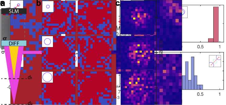
Figure 2: Tuning the spin correlation length by optical propagation. a) Schematic representation of the setup in two different distance configurations: $d_{1}$ in red and $d_{2}$ in orange, where the colored cones represent where the light reaching one CCD pixel comes from on the SLM. b) Simulation (first col) and experimental (second col) spin maps at three different imaging plane CCD-DIFF distances. The further away the plane, the wider the correlation. c) The amplitudes of the experimental transmission matrices at these same three distances.

A system of $N$ coupled spins is described by the Hamiltonian in Equation 1. For the Sherrington-Kirkpatrick model Nishimori (2001), the couplings ($J_{ij}$) are all-to-all random couplings, and are drawn from a Gaussian distribution. Finding the ground-state of Equation 1 is an NP-hard problem. This problem can be mapped onto a physical hardware thanks to coherent light-propagation in disordered medium. In this configuration, one can show that the transmitted intensity after a multiply-scattering medium takes the form Pierangeli et al. (2021):

$$H=-\sum_{i,j=1}^{N}J_{ij}\sigma_{i}\sigma_{j}=-I$$ (1)

with $J_{ij}=-\sum_{m}^{M}\Re{\overline{t_{im}}t_{jm}}$, where $m$ runs on the output modes and $t_{im}$ and $t_{jm}$ are transmission matrix ($T$) elements of the random medium. The matrix $T$ links the input modes on the spatial light modulator (SLM) ($E_{in}$) and the output modes on the camera ($E_{out}$) via $E_{out}=TE_{in}$ Popoff et al. (2010). The spins are encoded on the input modes (pixels) with a binary phase of $0$ and $\pi$, corresponding to $\pm 1$ spin states, respectively Pierangeli et al. (2021); Leonetti et al. (2021). Thanks to the physical system described in Figure 1 and using an optimization algorithm one can find the ground state of the Ising problem Pierangeli et al. (2019).

Figure 3: Controlling the interaction between spin clusters. a) Simulation (first columns) and experimental (second columns) spin ground states. b) TM amplitudes obtained summing all rows of the measured TM. Two isolated regions of magnetized spins (when optimizing over to two foci at the CCD plane) as displayed on the SLM (first row). As the distance between CCD and diffuser increases the extent of the magnetized regions also increases, the regions start to overlap and therefore interact (second row).

color=yellow]fig 3 the red looks faded compared to fig2

The couplings distribution ($J_{ij}$) can be tuned by using the knowledge of the transmission matrix $T$ Jacucci et al. (2022). In the present work, we use thin diffusive media Hobbs (2022); Sebbah (2001). These allow us —in contrast to thick scattering media Pierangeli et al. (2021, 2019, 2020)— to control the extent of spins contributing to the Hamiltonian. The further the camera is from the diffuser, the more the speckle pattern will spatially expand and the more the light coming from various input modes is mixed. In terms of couplings, it means that for a given input mode, the number of connected other input modes will increase as we get further from the medium. This effect can be used to control the spatial extent of the spins’ couplings. The insets in Figure 2 show a graphical representation of the amount of pixels contributing to the intensity on one single CCD pixel at two different distances. In terms of spin couplings, it means that for a given spin, the number of connected spins will increase as we get further from the medium. This effect can be used to control the spatial extent of the spin interaction. Remarkably, there exists two extreme points. The first one being when the distance is such that the speckle is fully developed, leading to an all-to-all coupled spin system (e.g. at position $d_{2}$ in Figure 2). The second one is when the distance is such that the spins are not coupled at all (e.g. at position $d_{1}$ in Figure 2). In this situation, the distance is so small that the light reaching the specific output can only come from one input mode (or SLM macro pixel). In other words, it is an Ising system of N decoupled spins.

Figure 4: Controlling frustration and replica symmetry breaking. a) Two regions of fixed size are increasingly getting closer on the SLM plane. Each point corresponds to ten replicas for one given distance. The graph shows the maximum of the probability distribution of the correlation between replicas $q_{max}$ as a function of the distance between the regions (in px on the CCD image). Replica-to-replica fluctuations vanish when the correlation is close to 1. b) and c) Histograms of the ground-state correlation for different replicas at maximum and minimum distance respectively.

In Reference Jacucci et al. (2022) we demonstrate the ability to tune the Hamiltonian of the system such that we obtain magnetized ground states for a given set of couplings. As shown in Figure 2, we apply the same technique to thin diffusers to tune the couplings such that we obtain a ground state with a localized magnetization. Figure 2a shows, for both simulations and experiments, three ground states for three different (increasing) distances between diffuser and CCD. As shown in Figure 2, we observe that the magnetized region is localized and has a finite size, whereas fully-magnetized ground states are expected for a thick medium Jacucci et al. (2022). Figure 2c offers a preview of the amplitude of the transmission matrix coefficients ($|T|$) for the three previous distances. It is evident here that the light that reaches this given CCD pixel (chosen for the optimization) comes from only a subset of the input modes (i.e. spins). Secondly, one can note that the interaction length between the spins grows with the distance to the diffuser (c.f. Figure 2c).

The ability to tune the spatial extent of the region where spins are mutually coupled allows us to create several clusters and explore the interactions between them by selecting two pixels at some distance, and optimizing over the sum of their intensities. We define the interaction area as the zone where the two regions overlap. The spins within this area contribute to both foci at the two different camera-pixels corresponding respectively to the two regions. Figure 3 displays an example of two regions, varying their distance and the interaction length. In detail, Figure 3a shows the ground states, for both simulations and experiments, obtained for the whole system (both regions) and for two different distances between diffuser and CCD. The first column shows the case where the two regions are not overlapping, the second column shows the case where the two regions are overlapping. Figure 3b shows the transmission matrix amplitudes for the two previous cases. We can also tune the overlap between spin clusters by keeping the distance $d$ fixed and by translating the two pixels on the CCD — effectively optimizing for two closer pixels.

We finally investigate the probability of the two interaction regions being magnetized in an uncorrelated way as their distance varies. When regions are not coupled, they are independent and the magnetization is thus the same $50\%$ of the time. When they get closer, their magnetization tends to be correlated. This is due the fact that the regions are not independent anymore, as there is an overlap between them, corresponding to a coupling between the two regions. To quantify the correlations between various replica, we defined—in analog manner as the Parisi order parameter Pierangeli et al. (2017); Ghofraniha et al. (2015); Mézard and Young (1992); Mézard et al. (1984); Parisi (1983)—the following metric for fully-magnetized spin configurations:

$$q_{\alpha\beta}=1-\frac{|\sum_{i=1}^{N}X^{\alpha}_{i}-X^{\beta}_{i}|}{N}$$

where $\alpha$ and $\beta$ refer to two replicas, $N$ is the number of spins in the region of interest and $X^{\alpha,\beta}_{i}\in\{-1,1\}$ are spin configurations. The zone of interest in which the correlation between replica ground states is calculated is a smaller region than the full input modes mask (c.f. green square in inset schematics of Figure 4a).

Figure 4a shows the correlation between replicas as a function of the distance between the two regions. The correlation is defined as the maximum of the probability distribution of the correlation between replicas $q_{max}$ (which is defined as $q_{\text{max}}=\text{argmax}_{q}P(q)$, where $P$ represents the distributioncolor=red]i need to renormalize for it to be a probability (1 must be the max) of the degree of correlation $q$ between ground states). The correlation is close to unity when replica-to-replica fluctuations drop to $0$. Figure 4b and Figure 4c show the histograms of the correlation between ground states of different replicas when the two regions are the furthest and the closest respectively. We observe that by increasing the overlap between the two areas —and therefore their interaction— the correlation increases, in analogy with the replica symmetry breaking transition, typical of random spin systems (c.f. Figure 4c). A simulation of our system can be found in the Appendix C, describing some conditions on the overlap for which one observes RSB-like behavior and what the assumptions on the couplings amplitude distribution are.

In short, we have observed and demonstrated experimental control over the interaction length of an Ising spin-glass system based on free-space optics and disordered media. We have also shown that we can control the interaction between two regions of spins and induce replica symmetry breaking.

The proposed system is a step towards encoding more complex Hamiltonians in hope of solving more complex NP-problems. It is also a new platform for studying replica symmetry breaking. Moreover, the degeneracy changing when regions interact means that the systems seems to develop long-range couplings from short-range couplings. This effect could be leveraged as a new type of annealing approach. Indeed, one could anneal a subset of the system and then — driven by the interaction — the whole system would anneal.

Furthermore, one could even consider generalizing this Ising system to a Hopfield system Leonetti et al. (2021) as our experimental setup is algorithm-agnostic and the spins are defined with a continuous encoding, therefore a continuous orientation of spins could be explored. Other platforms could also be envisioned, such as using multiple SLMs or using non-linear or more complex media to obtain more complex couplings distributions (bimodal, multimodal, etc).

Methods

Experimental setup. We evaluated experimentally our approach for controlling the couplings of the spin simulator (c.f. Figure 1) as well as its extension with the additions described below. A laser (Coherent Sapphire SF 532, $\lambda=532nm$) is directed onto a reflective phase-only, liquid-crystal SLM (Meadowlark Optics HSP192-532, $1920\times 1152$ pixels, aggregated into $N=256$ macro-pixels) divided into N macro-pixels (spins). The Fourier transform of the modulated light is projected on the objective back focal-plane (OBJ1, $10\times$, $\mathrm{NA}=0.1$) and focused on a scattering medium (DIFF). As a scattering, medium we used a surface-diffuser that is commercially available (Edmund, 12.5mm, 25°). In practice, using a thin volumetric diffuser or combining a surface diffuser and free-space propagation are equivalent in our scheme. The scattered light is then collected by a second objective (OBJ2, $20\times$, $\mathrm{NA}=0.4$) and the transmitted intensity is detected by a CCD camera (Basler acA2040-55$\mu$m, $2048\times 1536$ pixels). The spins and bias (from the TM Jacucci et al. (2022)) are encoded by a spatial light modulator (SLM) in a phase pattern whose binary part is sequentially updated until the ground-state is reached. Note that for the optimization any algorithm can be used, i.e., the setup is algorithm agnostic, as the advantage of the aforementioned simulator resides in the parallel measurements of the energy Pierangeli et al. (2021).

Transmission matrix calculation and ground-state search. The transmission matrix of the scattering medium was estimated as in Popoff et al. (2010). In detail, each row of the TM can be reconstructed by monitoring how the intensity on a given CCD pixel changes when a phase modulation is applied to the input patterns on the SLM. Those interferometry measurements provide the TM. Taking the phase conjugate of this matrix gives the SLM mask necessary for proper focusing Jacucci et al. (2022). The TM is sensitive to translations and rotations of the scattering medium as well as to the input and detection hardware. In this work, we define the stability-time as a variation within $10\%$ of it original value. This time (typically $\sim 120$ minutes) is long enough to run our experiments but for larger systems one would need more stable architectures. The ground-state search is conducted sequentially by means of the recurrent digital feedback. Computation starts from a random configuration of N binary macro-pixels (spins) on the SLM. The measured intensity distribution determines the feedback signal. At each iteration, an arbitrary batch of spins is randomly flipped if it increases the intensity at a chosen output mode. The batch size decreases over the optimization procedure, starting from $12\%$ of the pixels to a single pixel for the last $\sim 600$ iterations.

Numerical methods. The numerical model used in this work is a generalization of Pierangeli et al. (2021). The optical SG is numerically simulated by forming N pixel blocks (SLM plane). The initial optical field has a constant amplitude, and its phase is a random configuration of N binary phases, $\phi_{i}=0,\pi$. A gaussian i.i.d. transmission matrix T with random complex numbers is generated. At each iteration, a randomly selected single spin is flipped. The input phase is updated if the output total intensity increased after the linear propagation of the field. The bias in the numerical framework is calculated as in the experiment by starting from the knowledge of T. Numerical evaluation of $I_{T}$ corresponds to a measurement with a detector in a noiseless system. In general, within this scheme, $\sim 10N$ iterations are sufficient for a good convergence, i.e., when focus intensity reaches a plateau. All codes are implemented in MATLAB on an Intel processor with 14 cores running at 3.7 GHz and supported by 64 GB ram.

References

- Parisi (2006) G. Parisi, Proceedings of the National Academy of Sciences 103, 7948 (2006), https://www.pnas.org/doi/pdf/10.1073/pnas.0601120103 .
- Takeda et al. (2017) Y. Takeda, S. Tamate, Y. Yamamoto, H. Takesue, T. Inagaki, and S. Utsunomiya, Quantum Science and Technology 3, 014004 (2017).
- Maccari et al. (2019) I. Maccari, L. Benfatto, and C. Castellani, Phys. Rev. B 99, 104509 (2019).
- Das and Chakrabarti (2008) A. Das and B. K. Chakrabarti, Rev. Mod. Phys. 80, 1061 (2008).
- Goto et al. (2019) H. Goto, K. Tatsumura, and A. R. Dixon, Science Advances 5, eaav2372 (2019), https://www.science.org/doi/pdf/10.1126/sciadv.aav2372 .
- Lenstra and Kan (1975) J. K. Lenstra and A. H. G. R. Kan, Journal of the Operational Research Society 26, 717 (1975), https://doi.org/10.1057/jors.1975.151 .
- Lucas (2014) A. Lucas, Frontiers in Physics 2, 5 (2014).
- Garey and Johnson (1990) M. R. Garey and D. S. Johnson, Computers and Intractability; A Guide to the Theory of NP-Completeness (W. H. Freeman & Co., USA, 1990).
- Barahona (1982) F. Barahona, Journal of Physics A: Mathematical and General 15, 3241 (1982).
- Bachas (1984) C. P. Bachas, Journal of Physics A: Mathematical and General 17, L709 (1984).
- Nishimori (2001) N. Nishimori, Statistical Physics of Spin Glasses and In- formation Processing: An Introduction (Clarendon Press-Oxford, 2001).
- Fu and Anderson (1986) Y. Fu and P. Anderson, Journal of Physics A 19, 1605 (1986).
- Sherrington and Kirkpatrick (1975) D. Sherrington and S. Kirkpatrick, Phys. Rev. Lett. 35, 1792 (1975).
- Jacucci et al. (2022) G. Jacucci, L. Delloye, D. Pierangeli, M. Rafayelyan, C. Conti, and S. Gigan, Phys. Rev. A 105, 033502 (2022).
- Pierangeli et al. (2019) D. Pierangeli, G. Marcucci, and C. Conti, Phys. Rev. Lett. 122, 213902 (2019).
- Pierangeli et al. (2021) D. Pierangeli, M. Rafayelyan, C. Conti, and S. Gigan, Phys. Rev. Applied 15, 034087 (2021).
- Pierangeli et al. (2020) D. Pierangeli, G. Marcucci, and C. Conti, Optica 7, 1535 (2020).
- Tommasi et al. (2016) F. Tommasi, E. Ignesti, S. Lepri, and S. Cavalieri, Scientific Reports 6, 37113 (2016).
- Ghofraniha et al. (2015) N. Ghofraniha, I. Viola, F. Di Maria, G. Barbarella, G. Gigli, L. Leuzzi, and C. Conti, Nature Communications 6, 6058 (2015).
- Johnson et al. (2011) M. W. Johnson, M. H. S. Amin, S. Gildert, T. Lanting, F. Hamze, N. Dickson, R. Harris, A. J. Berkley, J. Johansson, P. Bunyk, E. M. Chapple, C. Enderud, J. P. Hilton, K. Karimi, E. Ladizinsky, N. Ladizinsky, T. Oh, I. Perminov, C. Rich, M. C. Thom, E. Tolkacheva, C. J. S. Truncik, S. Uchaikin, J. Wang, B. Wilson, and G. Rose, Nature 473, 194 (2011).
- Boixo et al. (2014) S. Boixo, T. F. Rønnow, S. V. Isakov, Z. Wang, D. Wecker, D. A. Lidar, J. M. Martinis, and M. Troyer, Nature Physics 10, 218 (2014).
- Berloff et al. (2017) N. G. Berloff, M. Silva, K. Kalinin, A. Askitopoulos, J. D. Töpfer, P. Cilibrizzi, W. Langbein, and P. G. Lagoudakis, Nature Materials 16, 1120 (2017).
- Kalinin et al. (2020) K. P. Kalinin, A. Amo, J. Bloch, and N. G. Berloff, Nanophotonics 9, 4127 (2020).
- Harris et al. (2018) R. Harris, Y. Sato, A. J. Berkley, M. Reis, F. Altomare, M. H. Amin, K. Boothby, P. Bunyk, C. Deng, C. Enderud, S. Huang, E. Hoskinson, M. W. Johnson, E. Ladizinsky, N. Ladizinsky, T. Lanting, R. Li, T. Medina, R. Molavi, R. Neufeld, T. Oh, I. Pavlov, I. Perminov, G. Poulin-Lamarre, C. Rich, A. Smirnov, L. Swenson, N. Tsai, M. Volkmann, J. Whittaker, and J. Yao, Science 361, 162 (2018).
- Hamerly et al. (2019) R. Hamerly, T. Inagaki, P. L. McMahon, D. Venturelli, A. Marandi, T. Onodera, E. Ng, C. Langrock, K. Inaba, T. Honjo, K. Enbutsu, T. Umeki, R. Kasahara, S. Utsunomiya, S. Kako, K. ichi Kawarabayashi, R. L. Byer, M. M. Fejer, H. Mabuchi, D. Englund, E. Rieffel, H. Takesue, and Y. Yamamoto, Science Advances 5, 0823 (2019).
- Pierangeli et al. (2017) D. Pierangeli, A. Tavani, F. Di Mei, A. J. Agranat, C. Conti, and E. DelRe, Nature Communications 8, 1501 (2017).
- Waidyasooriya et al. (2022) H. M. Waidyasooriya, Y. Ohma, and M. Hariyama, in 2022 IEEE 15th International Symposium on Embedded Multicore/Many-core Systems-on-Chip (MCSoC) (2022) pp. 195–199.
- Marandi et al. (2014) A. Marandi, Z. Wang, K. Takata, R. L. Byer, and Y. Yamamoto, Nature Photonics 8, 937 (2014).
- Haribara et al. (2016) Y. Haribara, S. Utsunomiya, and Y. Yamamoto, Lecture Notes in Physics , 251–262 (2016).
- McMahon et al. (2016) P. L. McMahon, A. Marandi, Y. Haribara, R. Hamerly, C. Langrock, S. Tamate, T. Inagaki, H. Takesue, S. Utsunomiya, K. Aihara, R. L. Byer, M. M. Fejer, H. Mabuchi, and Y. Yamamoto, Science 354, 614 (2016).
- Inagaki et al. (2016a) T. Inagaki, Y. Haribara, K. Igarashi, T. Sonobe, S. Tamate, T. Honjo, A. Marandi, P. L. McMahon, T. Umeki, K. Enbutsu, O. Tadanaga, H. Takenouchi, K. Aihara, K. ichi Kawarabayashi, K. Inoue, S. Utsunomiya, and H. Takesue, Science 354, 603 (2016a).
- Böhm et al. (2019) F. Böhm, G. Verschaffelt, and G. Van der Sande, Nature Communications 10, 3538 (2019).
- Takesue et al. (2020) H. Takesue, K. Inaba, T. Inagaki, T. Ikuta, Y. Yamada, T. Honjo, T. Kazama, K. Enbutsu, T. Umeki, and R. Kasahara, Phys. Rev. Applied 13, 054059 (2020).
- Honjo et al. (2021) T. Honjo, T. Sonobe, K. Inaba, T. Inagaki, T. Ikuta, Y. Yamada, T. Kazama, K. Enbutsu, T. Umeki, R. Kasahara, K. ichi Kawarabayashi, and H. Takesue, Science Advances 7, 0952 (2021).
- Nixon et al. (2013) M. Nixon, E. Ronen, A. A. Friesem, and N. Davidson, Phys. Rev. Lett. 110, 184102 (2013).
- Hamerly et al. (2020) R. Hamerly, T. Inagaki, P. L. McMahon, D. Venturelli, A. Marandi, D. R. Englund, and Y. Yamamoto, in AI and Optical Data Sciences, Vol. 11299, edited by B. Jalali and K. ichi Kitayama, International Society for Optics and Photonics (SPIE, 2020) pp. 42 – 48.
- Calvanese Strinati et al. (2021) M. Calvanese Strinati, L. Bello, E. G. Dalla Torre, and A. Pe’er, Phys. Rev. Lett. 126, 143901 (2021).
- Gershenzon et al. (2020) I. Gershenzon, G. Arwas, S. Gadasi, C. Tradonsky, A. Friesem, O. Raz, and N. Davidson, Nanophotonics 9, 4117 (2020).
- Edri et al. (2021) H. Edri, B. Raz, G. Fleurov, R. Ozeri, and N. Davidson, New Journal of Physics 23, 053005 (2021).
- Inagaki et al. (2016b) T. Inagaki, K. Inaba, R. Hamerly, K. Inoue, Y. Yamamoto, and H. Takesue, Nature Photonics 10, 415 (2016b).
- Honjo et al. (2022) T. Honjo, K. Inaba, T. Inagaki, T. Ikuta, Y. Yamada, and H. Takesue, in 2022 IEEE 22nd International Conference on Nanotechnology (NANO) (2022) pp. 405–408.
- Cen et al. (2022) Q. Cen, H. Ding, T. Hao, S. Guan, Z. Qin, J. Lyu, W. Li, N. Zhu, K. Xu, Y. Dai, and M. Li, Light: Science & Applications 11, 333 (2022).
- (43) W. Sun, W. Zhang, Y. Liu, Q. Liu, and Z. He, 47, 1498.
- Kumar et al. (a) S. Kumar, H. Zhang, and Y.-P. Huang, 3, 1 (a).
- Kumar et al. (b) S. Kumar, Z. Li, T. Bu, C. Qu, and Y. Huang, 6, 1 (b).
- (46) J. Huang, Y. Fang, and Z. Ruan, 4, 1.
- (47) Y. Fang, J. Huang, and Z. Ruan, 127, 043902, 2011.02771 .
- Mézard et al. (1984) M. Mézard, G. Parisi, N. Sourlas, G. Toulouse, and M. Virasoro, Journal de Physique 45, 843 (1984).
- (49) M. Mezard, G. Parisi, and M. Virasoro, Spin Glass Theory and Beyond: An Introduction to the Replica Method and Its Applications, World Scientific Lecture Notes in Physics, Vol. 9 (WORLD SCIENTIFIC).
- Popoff et al. (2010) S. M. Popoff, G. Lerosey, R. Carminati, M. Fink, A. C. Boccara, and S. Gigan, Phys. Rev. Lett. 104, 100601 (2010).
- Leonetti et al. (2021) M. Leonetti, E. Hörmann, L. Leuzzi, G. Parisi, and G. Ruocco, Proceedings of the National Academy of Sciences 118 (2021).
- Hobbs (2022) P. C. Hobbs, Building electro-optical systems: making it all work (John Wiley & Sons, 2022).
- Sebbah (2001) P. Sebbah, Waves and imaging through complex media (Springer Science & Business Media, 2001).
- Mézard and Young (1992) M. Mézard and A. P. Young, Europhysics Letters 18, 653 (1992).
- Mézard et al. (1984) M. Mézard, G. Parisi, N. Sourlas, G. Toulouse, and M. Virasoro, Phys. Rev. Lett. 52, 1156 (1984).
- Parisi (1983) G. Parisi, Phys. Rev. Lett. 50, 1946 (1983).