Thermoelectric response in nodal-point semimetals

Abstract

In this review, we discuss the thermoelectric properties in nodal-point semimetals with two bands. For the two-dimensional (2D) case, we show that the expressions of the thermoelectric coefficients take different values depending on the nature of the scattering mechanism responsible for transport, by considering examples of short-ranged disorder potential and screened charged impurities. An anisotropy in the energy dispersion spectrum invariably affects the thermopower quite significantly, as illustrated by the results for a node of semi-Dirac semimetal and a single valley of graphene. We also consider the scenario when a magnetic field of magnitude $B$ is applied perpendicular to the plane of the 2D semimetal. The computations for three-dimensional (3D) cases necessarily involve the inclusion of nontrivial Berry phase effects. In addition to demonstrating the expressions for the response tensors, we discuss the exotic behaviour observed in planar Hall and planar thermal Hall set-ups.

I Introduction

The measurement of the thermoelectric effects is one of the most widely used experimental probes for investigating transport mechanisms in metals, semimetals, and semiconductors. The behaviour of thermopower has proved to be a powerful and versatile tool in characterizing material properties as it provides information complementary to that obtained from electrical resistivity measurements, for example, by shedding light on both the conduction processes and thermodynamics. In this review, we will elucidate the derivation of the analytical expressions for the thermoelectric coefficients for the quasiparticles emerging in two-dimenstional (2D) and three-dimensional (3D) semimetals with a pair of bands. At a nodal-point of such a semimetal, the two bands cross each other giving a zero density of states right at the band-crossing point. We will consider the cases when an electric field $\mathbf{E}$ (or a temperature gradient ${\nabla}_{\mathbf{r}}T$) is applied externally across a sample. The thermoelectric coefficients take different values depending on the relaxation processes involved, which include short-ranged disorder and scattering off charged impurities. The results obtained using the Boltzmann equation approach turn out to be in good agreement with other theoretical approaches like the Kubo formula and the quantum Boltzmann equation. We will also discuss the situation when a magnetic field $\mathbf{B}$ is applied in addition. For the 2D cases, the direction of $\mathbf{B}$ is perpendicular to the plane of the semimetal. For the 3D cases, if the magnetic field has a parallel component along $\mathbf{E}$ or ${\nabla}_{\mathbf{r}}T$, we observe the so-called planar Hall or planar thermal Hall phenomenon. For a weak magnetic field, when the formation of the Landau levels can be ignored, we will continue to use the semiclassical Boltzmann formalism. However, this fails for strong magnetic fields, leading to quantized energy eigenvalues in the form of Landau levels. We deal with this quantizing magnetic field regime by using entropy to derive the form of the transport coefficients [1, 2]. In all our calculations, we consider a single node and focus on the cases when the relaxation time involves only the intranode scattering processes.

There is an extensive literature devoted to the study of the thermoelectric properties of 2D isotropic materials like graphene and related 2D Dirac materials [3, 4]. For 3D nodal-point semimetals, one needs to include the effects of a nontrivial Berry curvature [5, 6, 7, 8, 9, 10, 11, 12, 13, 14, 15]. The characterization of transport properties in isotropic Dirac/Weyl materials has spanned both 2D and 3D [3, 4, 16, 17, 18, 19, 20, 21, 22, 9, 23, 24, 25, 26, 27, 28]. Subsequently, the task of computing the thermoelectric properties in 2D anisotropic Dirac/Weyl materials, such as VO₂/TiO₃ [29, 30, 31], organic salts [32, 33], and deformed graphene [34, 35, 36, 37], has been taken up [38]. Such a system is represented by a semi-Dirac semimetal featuring two bands, whose low-energy bandstructure harbours a linear dispersion in one direction and a quadratic dispersion along the direction perpendicular to it. Since transport coefficients are determined by the bandstructure and the relevant scattering processes for the emergent quasiparticles, the anisotropic dispersion of the 2D semi-Dirac materials invariably leads to unconventional electric and magnetic properties, as opposed to the isotropic Weyl/Dirac systems [39, 40]. There also have been studies incorporating the 3D anisotropic cases [41, 11, 12]. In particular, the behaviour of the transport coefficients reflects how anisotropy can give rise to interesting field-, temperature-, and doping-dependence.

The review is organized as follows. In Sec. II and Sec. III, we outline the derivation of the semiclassical Boltzmann equations and the expressions of the transport coefficients under the relaxation time approximation. The second one expands on the first to include nontrivial Berry phase effects. Sec. IV—Sec. VIII consider the 2D cases, providing comparisons for linear-in-momentum isotropic (by considering a single valley of graphene) and hybrid/anisotropic (by considering semi-Dirac semimetal) dispersions. In Sec. IV, we provide the analytical expressions for thermoelectric coefficients in zero magnetic field, assuming a constant (i.e., independent of energy or momentum) relaxation time. In Sec. V, we discuss the form of the transport coefficients by using a relaxation time resulting from the scatterings off short-ranged disorder. This is followed by Sec. VI, where we consider a relaxation time caused by the presence of a screened Coulomb potential for the carriers, resulting from charged impurities. In Sec. VII and Sec. VIII, we add an external magnetic field directed along the line perpendicular to the plane of the 2D semimetals. These two sections elucidate the behaviour of the transport coefficients for the weak (non-quantizing) and strong regimes (i.e., when Landau levels emerge) of the strength external magnietic field, respectively. Finally, we conclude with a summary and outlook in Sec. X.

II Semiclassical Boltzmann equation for zero Berry curvature

Our fundamental understanding of electronic properties of crystalline solids is primarily based on the Bloch theory for periodic systems. One of the most widely used descriptions is the semiclassical theory for quasiparticle dynamics within a band supplemented by the simple and efficient framework of the Boltzmann transport equations. Hence, we review the Boltzmann’s transport theory which allows us to deal with dissipation and momentum relaxation of non-stationary electronic states in metals and semimetals. The task of computing a finite conductivity can be used a formalism based on the distribution function of quasiparticles. A system isolated from external influence reaches equilibrium through relaxation after some characteristic time, accompanied with an increase of entropy as can be explained using the tools of statistical physics. Considering a system in $d$ spatial dimensions, we define the distribution function (alternatively, the probability density function) $f_{n}(\mathbf{r},\mathbf{k},t)$ for the Bloch band (labelled by the index $n$) with the crystal momentum $\mathbf{k}$ and dispersion $\epsilon_{n}(\mathbf{k})$, such that

$$dN_{n}=g_{n}\,f_{n}(\mathbf{r},\mathbf{k},t)\,\frac{d^{d}\mathbf{k}}{(2\,\pi)^{d}}\,d^{d}\mathbf{r}$$ (1)

is the number of particles in an infinitesimal phase space volume $dV_{p}=\frac{d^{d}\mathbf{k}}{(2\,\pi)^{d}}\,d^{d}\mathbf{r}$ centered at $\left\{\mathbf{r},\mathbf{k}\right\}$ at time $t$, and $g_{n}$ is the degeneracy of the band. By definition, the distribution function $f_{n}$ is dimensionless. By performing integrals over the momentum space involving $f_{n}$ in the integrands, we can obtain various physical quantities. Let $\mathcal{Q}$ be the electric charge of a single quasiparticle and

$$\boldsymbol{v}_{n}({\mathbf{k}})=\frac{1}{\hbar}\,\nabla_{\mathbf{k}}\epsilon_{n}({\mathbf{k}})$$ (2)

be the Bloch velocity (or group velocity), with $\hbar$ denoting the reduced Planck’s constant.

In our set-up, we assume that the system is inhomogeneous on a large scale, and we are dividing it into subsystems which are approximately homogeneous. Then each of these subsystems can be characterized by the distribution function $f_{n}(\mathbf{r},\mathbf{k},t)$, which depends on the position of the corresponding subsystem. The Liouville’s theorem, which describes the evolution of the distribution function in phase space for a Hamiltonian system, states that $\frac{df_{n}}{dt}=0$. In other words, the distribution function is a probabilitiy distribution in the phase space and, because probability is locally conserved, it must obey a continuity equation just like an incompressible fluid. Consequently, in the course of the evolution of the probability distribution function governed by the Hamilton’s equations of motion, the probability does not change as we follow it along any trajectory in the phase space and, hence, represents an integral of motion. Liouville theorem stating that the distribution function remains constant. This follows from the fact that phase space volume does not change and particle number is conserved in phase space. If collisions are taken into consideration, Liouville’s theorem is violated and the distribution function is no longer constant along semiclassical phase space trajectories. Therefore, in order to explain dissipative transport phenomena resulting from scattering events, Ludwig Boltzmann modified the Liouville equation to

$$\frac{df_{n}}{dt}=\left[\frac{\partial f_{n}}{\partial t}\right]_{\text{coll}}$$

$$\Rightarrow \left(\partial_{t}+\dot{\mathbf{r}}\cdot\nabla_{\mathbf{r}}+\dot{\mathbf{k}}\cdot\nabla_{\mathbf{k}}\right)f_{n}=\left[\frac{\partial f_{n}}{\partial t}\right]_{\text{coll}}\,,$$ (3)

where the the right-hand-side contains the correction term $\left[\frac{\partial f_{n}}{\partial t}\right]_{\text{coll}}$ due to collisions added as a perturbation. We have denoted total time derivatives by the widely used convention of overhead dots. The collision term must be such that the distribution functions relaxes toward thermal equilibrium. Equations of this form generically represent kinetic equations.

The Hamilton’s equations of motion for Bloch electrons in electromagnetic fields are given by (cf. Chapter–12 of Ref. [42]):

$${\hbar}\,\dot{\mathbf{r}}=\partial_{\mathbf{k}}\epsilon_{n}({\mathbf{k}})\,,\quad\hbar\,\dot{\mathbf{k}}={\mathcal{Q}}\left({\mathbf{E}}+\frac{\dot{\mathbf{r}}\times{\mathbf{B}}}{c}\right),$$ (4)

where $\mathbf{E}$ and $\mathbf{B}$ are the externally applied electric applied electric and magnetic fields. Here, we have neglected the orbital magnetization of the Bloch wavepacket and the contributions from the spin-orbit interactions. Furthermore, we have assumed that the Bloch bands are topologically trivial. Using Eqs. (II) and (4), this leads to the kinetic equation

$$\left[\partial_{t}+{\boldsymbol{v}}_{n}\cdot\nabla_{\mathbf{r}}+\frac{\mathcal{Q}}{\hbar}\left(\mathbf{E}+\frac{{\boldsymbol{v}}_{n}\times{\mathbf{B}}}{c}\right)\cdot\nabla_{\mathbf{k}}\right]f_{n}=\left[\frac{\partial f_{n}}{\partial t}\right]_{\text{coll}}\,.$$ (5)

The terms on the left-hand-side are often denoted as the drift terms constituting the “co-moving” total time derivative. They are also sometimes referred to as the “streaming term” because it tells us how the quasiparticles move in the absence of collisions. On the other hand, the right-hand-side results from collisions and it is also often referred to as the collision integral. Due to this two sets of terms, two effects cause $f_{n}$ to evolve with time $t$:
(1) There is a smooth evolution arising from the drift and acceleration of the quasiparticles. Ignoring collisions, evolving from time $t$ to $t+\Delta t$, the new distribution $f_{n}(\mathbf{r},\mathbf{k},t+\Delta t)$ will be the old distribution $f_{n}(\mathbf{r}-\dot{\mathbf{r}}\,\Delta t,\mathbf{k}-\dot{\mathbf{k}}\,\Delta t,t)$. This part is the consequence of the Liouville’s theorem.
(2) Scattering processes cause discontinuous changes of the momentum $\mathbf{k}$ at some statistical rate.

One of the main assumptions of the Boltzmann transport equation is that particles can be treated semiclassically, obeying Newton’s laws of motion. Quantum mechanics enters into the equation only through the band-structure and the description of the collision term. Needless to say, $f_{n}(\mathbf{r},\mathbf{k},t)$ being a function of $\mathbf{r}$ and $\mathbf{k}$ simultaneously will not violate the uncertainty principle if the subsystems (into which the system is divided into) are large enough. In other words, the spatial variations and the temporal variations should occur at large distances (or long wavelengths denoted by $\lambda$) and small frequencies (denoted by $\omega$), respectively, i.e., for $\lambda\gg 2\,\pi/k_{F}$ and $\hbar\,\omega\ll E_{F}$, where $k_{F}$ and $E_{F}$ denote the Fermi momentum and Fermi energy, respectively. This scenario is feasible if we demand that the external perturbations do not vary rapidly in space. Hence, the Boltzmann equation formalism is a semiclassical description that does not account for very fast processes in small areas (which are the restrictions arising due to the uncertainty principle). The main idea behind the Boltzmann equation framework is that there are two time scales in the problem [43] — (1) the first is the time between two successive collisions ($\tau$), which is known as the scattering time or relaxation time; (2) the second is the collision time ($\tau_{\text{coll}}$) which is roughly the time it takes for a collision between quasiparticles to take place. In the regime where the condition $\tau\gg\tau_{\text{coll}}$ holds, then most of the time $f_{n}$ simply follows its Hamiltonian evolution, with occasional perturbations caused by the collision events.

In any system, the quasiparticles transport thermal energy (i.e., heat) simultaneously with electric charge. This is why transport of electric charge and heat are naturally interconnected. To demonstrate this connection, we now generalize the transport theory set up above. In order to derive the generalized Boltzmann equation, we consider a metal with weakly space-dependent temperature $T(\mathbf{r})$ and chemical potential $\mu(\mathbf{r})$. This necessitates the introduction of the electrochemical potential and the generalized (external) force field defined by

$$\eta(\mathbf{r})=\Phi(\mathbf{r})-\frac{\mu(\mathbf{r})}{\mathcal{Q}}\text{ and }\boldsymbol{\mathcal{E}}(\mathbf{r})=-\nabla_{\mathbf{r}}\eta(\mathbf{r})\,,$$ (6)

respectively, where $\Phi(\mathbf{r})$ is the electrostatic potential such that $\mathbf{E}=-\nabla_{\mathbf{r}}\Phi$. Hence, Eqs. (4) and (5) must be generalized to

$${\hbar}\,\dot{\mathbf{r}}=\partial_{\mathbf{k}}\epsilon_{n}({\mathbf{k}})\,,\quad\hbar\,\dot{\mathbf{k}}={\mathcal{Q}}\left(\boldsymbol{\mathcal{E}}+\frac{\dot{\mathbf{r}}\times{\mathbf{B}}}{c}\right)$$ (7)

and

$$\left[\partial_{t}+{\boldsymbol{v}}_{n}\cdot\nabla_{\mathbf{r}}+\frac{\mathcal{Q}}{\hbar}\left(\boldsymbol{\mathcal{E}}+\frac{{\boldsymbol{v}}_{n}\times{\mathbf{B}}}{c}\right)\cdot\nabla_{\mathbf{k}}\right]f_{n}=\left[\frac{\partial f_{n}}{\partial t}\right]_{\text{coll}}\,,$$ (8)

respectively.

In the following, we will consider a simple model of the collision integral which is known as the relaxation time approximation. The local value of the static distribution of the fermionic quasiparticles is given by the function

$$f^{(0)}_{n}(\mathbf{r},\mathbf{k})=\frac{1}{e^{\beta(\mathbf{r})\,\left\{\epsilon_{n}(\mathbf{k})-\mu(\mathbf{r})\right\}}+1}\,,$$ (9)

which describes a local equilibrium situation at the subsystem centred at position $\mathbf{r}$, at the local temperature $T(\mathbf{r})$, and with local chemical potential $\mu(\mathbf{r})$. We have used the symbol $\beta=1/(k_{B}\,T)$ (where $k_{B}$ is the Boltzmann constant), which is sometimes referred to as the inverse temperature. Now we make the ansatz

$$\left[\frac{\partial f_{n}}{\partial t}\right]_{\text{coll}}=-\frac{f_{n}(\mathbf{r},\mathbf{k},t)-f^{(0)}_{n}(\mathbf{r},\mathbf{k})}{\tau}\,,$$ (10)

where $\tau$ is called the relaxation time, which is generically $\mathbf{k}$-dependent. The relaxation time quantifies the characteristic time scale within which the system relaxes to equilibrium for the scattering processes relevant for the problem under consideration. The mean free path of the quasiparticles can be defined in terms of $\tau$ as

$$\ell=\tau\,v_{F}\,,$$ (11)

where $v_{F}$ is the Bloch velocity at the Fermi level. Two assumptions are made while applying the relaxation time approximation:
(1) The distribution function of the quasiparticles directly after a collision does not depend on their distribution function shortly before the collision. This assumption implies that collisions destroy all information about the non-equilibrium distribution function of the quasiparticles before the collision.
(2) Collisions do not change the shape of the equilibrium distribution function of the quasiparticles. This assumption actually saying that the collisions themselves are shaping the distribution function, or in other words, stabilizing the system as far as its thermodynamic equilibrium is concerned – consequently, they will not change it.

This approximation holds when we study processes close to equilibrium, i.e., when

$$|f_{n}(\mathbf{r},\mathbf{k},t)-f^{(0)}_{n}(\mathbf{r},\mathbf{k})|\ll f^{(0)}_{n}(\mathbf{r},\mathbf{k},t).$$

Therefore, in order to obtain a solution to the full Boltzmann equation, we assume a slight deviation quantified by

$$f_{n}(\mathbf{r},\mathbf{k},t)=f^{(0)}_{n}(\mathbf{r},\mathbf{k})+\delta f_{n}(\mathbf{r},\mathbf{k},t)\,,$$ (12)

with $f^{(0)}_{n}(\mathbf{r},\mathbf{k})$ given by Eq. (9). Observing that

$$\nabla_{\mathbf{r}}f^{(0)}_{n}(\mathbf{r},\mathbf{k}) =\left(\nabla_{\mathbf{r}}\mu+\frac{\epsilon_{n}-\mu}{T}\,\nabla_{\mathbf{r}}T\right)\left(-\frac{\partial f^{(0)}_{n}}{\partial\epsilon_{n}}\right),$$

$$\nabla_{\mathbf{k}}f^{(0)}_{n}(\mathbf{r},\mathbf{k}) =\hbar\,{\boldsymbol{v}}_{n}\,\frac{\partial f^{(0)}_{n}}{\partial\epsilon_{n}}\,,$$ (13)

the Boltzmann equation in Eq. (5) reduces to

$$\partial_{t}\delta f_{n}+{\boldsymbol{v}}_{n}\cdot{\nabla}_{\mathbf{r}}\,\delta f_{n}+\frac{\mathcal{Q}}{\hbar}\left(\mathbf{E}+\frac{{\boldsymbol{v}}_{n}\times{\mathbf{B}}}{c}\right)\cdot\nabla_{\mathbf{k}}\,\delta f_{n}+{\boldsymbol{v}}_{n}\cdot\left(-\frac{\epsilon_{n}-\mu}{T}\,\nabla_{\mathbf{r}}T+{\mathcal{Q}}\,\boldsymbol{\mathcal{E}}\right)\frac{\partial f^{(0)}_{n}}{\partial\epsilon_{n}}=-\frac{\delta f_{n}}{\tau}\,.$$ (14)

The form of the above equation reflects a caveat of the relaxation time approximation the Boltzmann equation [44, 45]. In the absence of any external fields or temperature and chemical potential gradients, Eq. (14) reduces to $\partial_{t}\delta f_{n}=-\delta f_{n}/\tau$, giving the solution $\delta f_{n}(t)=\delta f_{n}(t=0)\,\exp(-t/\tau)$. This result is physically incorrect because the total particle number is a collisional invariant. Since this approximation lacks particle number conservation (or electric charge conservation), this model cannot be used to determine the diffusion coefficient of the quasiparticles. However, this a defect of the relaxation time approximation does not affect the validity of our conclusions regarding various transport coefficients such as the electrical and thermal conductivities.

Let us consider a small region of solid with a fixed volume $dV$, centred around the position $\mathbf{r}$, where the temperature $T$ can be effectively taken to be constant. According to the first law of thermodynamics, we have

$$T\,d\mathcal{S}=dE-\mu\,dN$$ (15)

where $\mathcal{S}$ is the entropy, $E$ is the internal energy, and $N$ is the particle number. We divide by $dV$ to get the expression in terms of the corresponding volume densities:

$$T\,ds=d\epsilon-\mu\,d{\mathcal{N}}\,,$$ (16)

where $T\,ds$ represents the change in the thermal energy (or heat) density. The symbols $s$, $\epsilon$, and $\mathcal{N}$ denote the entropy density, internal energy density, and particle number density, respectively. The rate at which the thermal energy appears in the region $dV$ is just equal to $T\,ds$, leading to the average thermal current density expression of

$$\mathbf{J}^{Q}=T\,\mathbf{J}^{s}\,,$$ (17)

where $\mathbf{J}^{s}$ is the entropy current density. On the other hand, Eq. (16) leads to the relation

$$\mathbf{J}^{Q}=\mathbf{J}^{\epsilon}-\mu\,\mathbf{J}^{\mathcal{N}}$$ (18)

when expressed in terms of current densities, where $\mathbf{J}^{\epsilon}$ is the energy current density and $\mathbf{J}^{\mathcal{N}}$ is the particle number current density. If the quasiparticle number is not conserved, ${\mathbf{J}}^{\mathcal{N}}$ is not well-defined but $\mu=0$. For carriers with a conserved charge $\mathcal{Q}$ (for example, electrons with charge $e$) the particle current implies ${\mathbf{J}}={\mathcal{Q}}\,{\mathbf{J}}^{\mathcal{N}}$. For the latter case, by definition, we have

$$\mathbf{J}^{\mathcal{N}} =\sum_{n}g_{n}\int_{\text{ BZ}}\frac{d^{d}\mathbf{k}}{(2\,\pi)^{d}}\,\delta f_{n}(\mathbf{r},\mathbf{k},t)\,\boldsymbol{v}_{n}(\mathbf{k})\,,$$

$$\mathbf{J}^{\epsilon} =\sum_{n}g_{n}\int_{\text{ BZ}}\frac{d^{d}\mathbf{k}}{(2\,\pi)^{d}}\,\epsilon_{n}\,\delta f_{n}(\mathbf{r},\mathbf{k},t)\,\boldsymbol{v}_{n}(\mathbf{k})\,,$$ (19)

where the subscript “BZ” in each integral sign indicates that the integral has to be performed over the first Brillouin zone.

From the above discussions, we find that the average electrical and thermal currents in the system are given by

$${\mathbf{J}} ={\mathcal{Q}}\,{\mathbf{J}}^{\mathcal{N}}={\mathcal{Q}}\,\sum_{n}g_{n}\int_{\text{ BZ}}\frac{d^{d}\mathbf{k}}{(2\,\pi)^{d}}\,\delta f_{n}(\mathbf{r},\mathbf{k},t)\,\boldsymbol{v}_{n}(\mathbf{k})\,,$$

$$\mathbf{J}^{Q} =\sum_{n}g_{n}\int_{\text{BZ}}\frac{d^{d}\mathbf{k}}{(2\,\pi)^{d}}\left(\epsilon_{n}-\mu\right)\delta f_{n}(\mathbf{r},\mathbf{k},t)\,\boldsymbol{v}_{n}(\mathbf{k})\,.$$ (20)

The response matrix, which relates the resulting generalized currents to the driving forces, can be expressed as

$$\begin{pmatrix}J_{\alpha}\vspace{0.2 cm}\\ {J}^{Q}_{\alpha}\end{pmatrix} =\sum\limits_{\gamma}\begin{pmatrix}L_{\alpha\gamma}^{11}&L_{\alpha\gamma}^{12}\vspace{0.2 cm}\\ L_{\alpha\gamma}^{21}&L_{\alpha\gamma}^{22}\end{pmatrix}\begin{pmatrix}\mathcal{E}_{\gamma}\vspace{0.2 cm}\\ -{\partial_{r^{\gamma}}T}\end{pmatrix},$$ (21)

where the subscripts $\{\alpha,\gamma\}\in[1,d]$ indicate the Cartesian components of the current vectors and the transport tensors in $d$-dimensions. This gives us the Onsager matrix of transport coefficients.

For the case when $\mathbf{E}$, $\gradient_{\mathbf{r}}\mu$, and $\gradient_{\mathbf{r}}T$, and are time-independent, and with no magnetic field applied (i.e., $\mathbf{B}=0$), Eq. (14) reduces to

$$\partial_{t}\delta f_{n}+{\boldsymbol{v}}_{n}\cdot{\nabla}_{\mathbf{r}}\,\delta f_{n}+{\boldsymbol{v}}_{n}\cdot\left(\frac{\mu-\epsilon_{n}}{T}\,\nabla_{\mathbf{r}}T+{\mathcal{Q}}\,\boldsymbol{\mathcal{E}}\right)\frac{\partial f^{(0)}_{n}}{\partial\epsilon_{n}}$$

$$=-\frac{\delta f_{n}}{\tau}\,.$$ (22)

We can assume the solution $\delta f_{n}$ not to have any explicit time dependence since the applied fields and gradients are time-independent leading to $\partial_{t}\delta f_{n}=0$. Furthermore, we note that the inhomogeneous term in Eq. (II) involves $\boldsymbol{\mathcal{E}}$ and $\nabla_{\mathbf{r}}T$, implying that $\delta f_{n}$ is proportional to these quantities. Since we are forced to consider the external fields to be slowly varying in space, ${\nabla}_{\mathbf{r}}\,\delta f_{n}$ is the second order in the smallness parameter which might be used to parametrize the smallness of $\boldsymbol{\mathcal{E}}$ and $\nabla_{\mathbf{r}}T$. Therefore, to the leading lowest order in this smallness parameter, the so-called linearized Boltzmann equation is obtained as

$$\delta f_{n}=\tau\,{\boldsymbol{v}}_{n}\cdot\left(\frac{\epsilon_{n}-\mu}{T}\,\nabla_{\mathbf{r}}T-{\mathcal{Q}}\,\boldsymbol{\mathcal{E}}\right)\frac{\partial f^{(0)}_{n}}{\partial\epsilon_{n}}$$ (23)

for Eq. (14).

Plugging the results from Eq. (23) in Eq. (II), and setting $\mathcal{Q}=-e$ (which is the charge of an electron), we get

$$L_{\alpha\gamma}^{11}=-e^{2}\,\sum_{n}g_{n}\int_{\text{ BZ}}\frac{d^{d}\mathbf{k}}{(2\,\pi)^{d}}\,\tau\,\frac{\partial f^{(0)}_{n}}{\partial\epsilon_{n}}\,\,{{v}_{n}}_{\alpha}\,{{v}_{n}}_{\gamma}\,,$$

$$L_{\alpha\gamma}^{21}=T\,L_{\alpha\gamma}^{12}$$

$$=e\,\sum_{n}g_{n}\int_{\text{ BZ}}\frac{d^{d}\mathbf{k}}{(2\,\pi)^{d}}\,\tau\,\frac{\partial f^{(0)}_{n}}{\partial\epsilon_{n}}\,\,{{v}_{n}}_{\alpha}\,{{v}_{n}}_{\gamma}\left(\epsilon_{n}-\mu\right),$$

$$L_{\alpha\gamma}^{22}=-\sum_{n}g_{n}\int_{\text{ BZ}}\frac{d^{d}\mathbf{k}}{(2\,\pi)^{d}}\,\tau\,\frac{\partial f^{(0)}_{n}}{\partial\epsilon_{n}}\,\,{{v}_{n}}_{\alpha}\,{{v}_{n}}_{\gamma}\frac{\left(\epsilon_{n}-\mu\right)^{2}}{T}.$$ (24)

We note that the relation $L_{\alpha\gamma}^{12}=T\,L_{\alpha\gamma}^{21}$ between the off-diagonal transport coefficient tensors is a generic property that holds for any pair of cross transport coefficients and, as shown by Onsager, is a consequence of microscopic reversibility [46].

Using the condensed symbol

$${\mathcal{L}}_{\alpha\gamma}^{(\zeta)} =-e^{2}\sum_{n}g_{n}\int_{\text{ BZ}}\frac{d^{d}\mathbf{k}}{(2\,\pi)^{d}}\,\tau\,\frac{\partial f^{(0)}_{n}}{\partial\epsilon_{n}}\,\,{{v}_{n}}_{\alpha}\,{{v}_{n}}_{\gamma}\left(\epsilon_{n}-\mu\right)^{\zeta},$$ (25)

where $\zeta\in\{0,1,2\}$, the thermoelectric transport coefficient tensors are given by

$$L_{\alpha\gamma}^{11}=\mathcal{L}_{\alpha}^{(0)}\,,\quad L_{\alpha\gamma}^{21}=T\,L_{\alpha\gamma}^{12}=\frac{-\mathcal{L}_{\alpha\gamma}^{(1)}}{e}\,,$$

$$L_{\alpha\gamma}^{22}=\frac{\mathcal{L}_{\alpha\gamma}^{(2)}}{e^{2}\,T}\,.$$ (26)

The thermal conductivity is measured under the conditions when there is no electric current. To obtain this, it is convenient to transform Eq. (21) into a more convenient form as follows [44, 42]:

$$\begin{pmatrix}\mathcal{E}_{\alpha}\vspace{0.2 cm}\\ {J}^{Q}_{\alpha}\end{pmatrix} =\sum\limits_{\gamma}\begin{pmatrix}\rho_{\alpha\gamma}&S_{\alpha\gamma}\vspace{0.2 cm}\\ \Pi_{\alpha\gamma}&-\kappa_{\alpha\gamma}\end{pmatrix}\begin{pmatrix}J_{\gamma}\vspace{0.2 cm}\\ \partial_{r^{\gamma}}T\end{pmatrix}\,,$$ (27)

where
(1) $\rho$ is the resistivity tensor such that $\mathcal{E}_{\alpha}=\rho_{\alpha\gamma}\,J_{\gamma}$ under the condition $\nabla_{\mathbf{r}}T=0$;
(2) $S$ is the thermopower tensor (also known as the Seebeck coefficient) such that $\mathcal{E}_{\alpha}=S_{\alpha\gamma}\,\partial_{r^{\gamma}}T$ under the condition $\mathbf{J}=0$;
(3) $\Pi$ is the Peltier coefficient such that ${J}^{Q}_{\alpha}=\Pi_{\alpha\gamma}\,J_{\gamma}$ under the condition $\nabla_{\mathbf{r}}T=0$;
(4) $\kappa$ is the thermal conductivity tensor such that ${J}^{Q}_{\alpha}=-\kappa_{\alpha\gamma}\,\partial_{r^{\gamma}}T$ under the condition $\mathbf{J}=0$.
All the above ingredients allow us to formulate the final expressions for the electrical conductivity tensor $\sigma$, $S$, $\Pi$, and $\kappa$ as follows [42, 44]:

$$\sigma_{\alpha\gamma}=L_{\alpha\gamma}^{11}\,,\quad S_{\alpha\gamma}=\sum\limits_{\alpha^{\prime}}\left(L^{11}\right)^{-1}_{\alpha\alpha^{\prime}}L_{\alpha^{\prime}\gamma}^{12}\,,$$

$$\Pi_{\alpha\gamma}=\sum\limits_{\alpha^{\prime}}L_{\alpha\alpha^{\prime}}^{21}\,\left(L^{11}\right)^{-1}_{\alpha^{\prime}\gamma}\,,$$

$$\kappa_{\alpha\gamma}=L_{\alpha\gamma}^{22}-\sum\limits_{\alpha^{\prime},\,\gamma^{\prime}}L_{\alpha\alpha^{\prime}}^{21}\left(L^{11}\right)^{-1}_{\alpha^{\prime}\gamma^{\prime}}L_{\gamma^{\prime}\gamma}^{12}\,.$$ (28)

For the time-dependent case with no magnetic field, we get the dc resitivity and dc conductivity.

III Semiclassical Boltzmann equation for 3D nodal-point semimetals with nonzero Berry curvature

In the presence of a nontrivial topological charge in the bandstructure, the Boltzmann equation of Eq. (5) will get modified. We specifically focus on 3D nodal-point semimetals with nonzero Chern numbers. The Nielson-Ninomiya theorem [47] imposes the condition that the nodes come in pairs such that each pair carry Chern numbers which are equal in magnitude but opposite in signs. The sign of the monopole charge is often referred to as the chirality of the corresponding node.

Considering transport for a single node of chirality $\chi$ in a 3D nodal-point semimetal, Eq. (7) will get modified to [48, 49]

$${\hbar}\,\dot{\mathbf{r}}=\partial_{\mathbf{k}}\epsilon_{n}(\mathbf{k})-\hbar\,\dot{\mathbf{k}}\crossproduct\mathbf{\Omega}_{\chi,n}\,,\quad\hbar\,\dot{\mathbf{k}}={\mathcal{Q}}\left(\boldsymbol{\mathcal{E}}+\frac{\dot{\mathbf{r}}\crossproduct{\mathbf{B}}}{c}\right),$$ (29)

where $\mathbf{\Omega}_{\chi,n}(\mathbf{k})$ is the Berry curvature of the node, which is a pseudovector expressed by

$$\mathbf{\Omega}_{\chi,n}(\mathbf{k})=i\left\langle\nabla_{\mathbf{k}}u^{\chi}_{n}(\mathbf{k})\right|\crossproduct\left|\nabla_{\mathbf{k}}u_{n}^{\chi}(\mathbf{k})\right\rangle.$$ (30)

The Berry curvature arises from the Berry phases generated by $|u_{n}^{\chi}(\mathbf{k})\rangle$, where $\{|u_{n}^{\chi}(\mathbf{k})\rangle\}$ denotes the set of orthonormal Bloch cell eigenstates for the one-particle Hamiltonian $H_{\chi}(\mathbf{k})$ representing the low-energy effective description of the node with band energies $\{\epsilon_{n}\}$. It can be checked that $\mathbf{\Omega}_{\chi,n}$ is proportional to $\chi$ and, hence, it has opposite signs for an energy band with index $n$ at nodes of opposite chiralities. Furthermore, in the presence of a nontrivial topology, a weak nonquantizing magnetic field $\mathbf{B}$ necessitates the introduction of the shifted energy [22, 48, 50]

$$\tilde{\epsilon}_{n}(\mathbf{k})=\epsilon_{n}(\mathbf{k})-{\boldsymbol{m}}_{\chi,n}(\mathbf{k})\cdot{\mathbf{B}}(\mathbf{r},t)\,,$$ (31)

where

$${\boldsymbol{m}}_{\chi,n}(\mathbf{k})=\frac{i\,\mathcal{Q}}{2\,\hbar}\left\langle\nabla_{\mathbf{k}}u^{\chi}_{n}(\mathbf{k})\right|\crossproduct\left[H_{\chi}(\mathbf{k})-\epsilon_{n}(\mathbf{k})\right]\left|\nabla_{\mathbf{k}}u_{n}^{\chi}(\mathbf{k})\right\rangle$$ (32)

is the intrinsic magnetic moment generated by the Berry phase. Similar to $\mathbf{\Omega}_{\chi,n}$, the orbital moment is an intrinsic property of the band — it depends only on the Bloch wavefunctions. In fact, under symmetry operations, ${\boldsymbol{m}}_{\chi,n}$ transforms exactly like the Berry curvature. The orbital magnetic moment behaves exactly like the electron spin and, in presence of nonzero $\mathbf{B}$, it couples to the magnetic field through a Zeeman-like term — that is the reason behind the shift in energy eigenvalues. This necessitates redefining the Bloch velocity as

$$\tilde{\boldsymbol{v}}_{n}=\frac{1}{\hbar}\,\nabla_{\mathbf{k}}\tilde{\epsilon}_{n}({\mathbf{k}})\,.$$ (33)

The two coupled equations in Eq. (29) can be solved to obtain

$$\dot{\mathbf{r}} =D_{\chi,n}^{-1}\left[{\tilde{\boldsymbol{v}}}_{n}-\frac{\mathcal{Q}}{\hbar}\,\boldsymbol{\mathcal{E}}\crossproduct\mathbf{\Omega}_{\chi,n}-\frac{\mathcal{Q}}{c}\left(\mathbf{\Omega}_{\chi,n}\cdot{\tilde{\boldsymbol{v}}}_{n}\right)\mathbf{B}\right],$$

$$\hbar\,\mathbf{\dot{k}} =D_{\chi,n}^{-1}\,\mathcal{Q}\left[\boldsymbol{\mathcal{E}}+\frac{{\tilde{\boldsymbol{v}}}_{n}\crossproduct\mathbf{B}}{c}-\frac{\mathcal{Q}}{c}\,\left(\boldsymbol{\mathcal{E}}\cdot{\mathbf{B}}\right)\mathbf{\Omega}_{\chi,n}\right],$$ (34)

where

$$D_{\chi,n}^{-1}=1-\frac{\mathcal{Q}}{\hbar\,c}\,{\mathbf{B}}\cdot\mathbf{\Omega}_{\chi,n}\,.$$ (35)

The physical significance of the function $D_{\chi,n}$ can be understood as follows. Xiao et al. [22] observed that the Liouville’s theorem on the conservation of phase space volume element $dV_{p}$ is violated by the Berry phase in the semiclassical dynamics of Bloch electrons. This breakdown of the Liouville’s theorem is remedied by introducing a modified density of states in the phase space such that the number of states in the volume element $D_{\chi,n}^{-1}\,dV_{p}$ remains conserved. In other words, based on the modifications in the presence of nonzero Berry phases, the classical phase-space probability density is now given by [49, 22, 51, 52]

$$F_{n}(\mathbf{r},\mathbf{k},t)=D_{\chi,n}^{-1}(\mathbf{r},\mathbf{k})\,f_{n}(\mathbf{r},\mathbf{k},t)\,.$$ (36)

This implies that the probability conservation, in the absence of collisions, is equivalent to $F_{n}$ satisfying the continuity equation in the phase space, viz., $\frac{dF_{n}}{dt}=0$.

Incorporating all these ingredients, Eq. (8) should be modified to [53, 54]

$$D_{\chi,n}\,\left[\partial_{t}+\left\{{\tilde{\boldsymbol{v}}}_{n}-\frac{\mathcal{Q}}{\hbar}\,\boldsymbol{\mathcal{E}}\crossproduct\mathbf{\Omega}_{\chi,n}-\frac{\mathcal{Q}}{\hbar\,c}\left(\mathbf{\Omega}_{\chi,n}\cdot{\tilde{\boldsymbol{v}}}_{n}\right)\mathbf{B}\right\}\cdot\nabla_{\mathbf{r}}+\frac{\mathcal{Q}}{\hbar}\left(\boldsymbol{\mathcal{E}}+\frac{{\tilde{\boldsymbol{v}}}_{n}\crossproduct{\mathbf{B}}}{c}\right)\cdot\nabla_{\mathbf{k}}-\frac{\mathcal{Q}^{2}}{\hbar^{2}\,c}\,\left(\boldsymbol{\mathcal{E}}\cdot{\mathbf{B}}\right)\mathbf{\Omega}_{\chi,n}\cdot\nabla_{\mathbf{k}}\right]f_{n}$$

$$\,=\frac{f^{(0)}_{n}(\mathbf{r},\mathbf{k})-f_{n}(\mathbf{r},\mathbf{k},t)}{\tau(\mathbf{k})}\,,$$ (37)

respectively. We would like to point out that here $f^{(0)}_{n}$ is a function of $\tilde{\epsilon}_{n}$, i.e., $f^{(0)}_{n}(\mathbf{r},\mathbf{k})=\left[e^{\beta(\mathbf{r})\,\left\{\tilde{\epsilon}_{n}(\mathbf{k})-\mu(\mathbf{r})\right\}}+1\right]^{-1}$. For the sake of simplicity, here we have have assumed that only intranode scatterings are relevant, contributing to $\tau$, ignoring the internode processes. It is important to note that we have not assumed $|\mathbf{B}|$ to be very small. To solve the above equation, we need to make an appropriate ansatz, as outlined in (a) Refs. [55, 54] for planar Hall effect; and (b) Ref. [56] for planar thermal Hall effect.

In order to obtain a solution to the full Boltzmann equation in time-independent scenarios, for small values of $\mathbf{E}$, $\nabla_{\mathbf{r}}\mu$, and $\nabla_{\mathbf{r}}T$, we assume a slight deviation $\delta f_{n}(\mathbf{r},\mathbf{k})$ from the equilibrium distribution of the quasiparticles, which does not have any explicit time-dependence since the applied fields and gradients are time-independent. Hence, the non-equilibrium time-independent distribution function is assumed to be of the form shown in Eq. (12). The magnetic field, however, is not assumed to be small. It is reasonable to have assumed the solution $\delta f_{n}$ not to have any explicit time-dependence since the applied fields and gradients are time-independent. The gradients of equilibrium distribution function $f^{(0)}_{n}$ evaluate to Eq. (II). In the following, we will consider a uniform chemical potential, such that $\nabla_{\mathbf{r}}\mu=0$, as we are mainly intersted in the interplay of $\mathbf{E}$ (or $\nabla_{\mathbf{r}}T$) and $\mathbf{B}$. We assume that all of the quantities $\mathbf{E}$, $\nabla_{\mathbf{r}}T$, and the resulting $\delta f_{n}$ are of the same order of smallness. The spatial gradient $\nabla_{\mathbf{r}}f^{(0)}_{n}$ is parallel to the thermal gradient $\nabla_{\mathbf{r}}T$, and we consider situations where $\mathbf{E}$ and $\nabla_{\mathbf{r}}T$ to be along the same direction. Hence, the term $\mathcal{Q}\left({\mathbf{E}}\crossproduct\mathbf{\Omega}^{\chi}_{n}\right)\cdot\nabla_{\mathbf{r}}f^{(0)}_{n}$ in Eq. (III) gives zero.

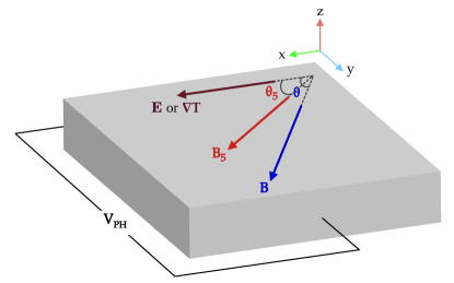
Figure 1: Schematics showing the planar Hall/thermal Hall experimental set-up, where the sample is subjected to an external electric field $E\,{\mathbf{\hat{x}}}$/temperature gradient $\partial_{x}T\,{\mathbf{\hat{x}}}$. An external magnetic field $\mathbf{B}$ is applied such that it makes an angle $\theta$ with the existing electric field/temperature gradient. The resulting planar Hall/thermal Hall voltage generated along the $y$-axis is indicated by the symbol $V_{\rm PH}$.

The particle current density of Eq. (18) is equal to ${\mathbf{J}}^{\chi}/{\mathcal{Q}}$ contributed by the single node, where ${\mathbf{J}}^{\chi}$ has a circulating component in the form of the orbital magnetization current [57]

$${\mathbf{J}}^{\chi,\rm mag}=\sum_{n}g_{n}\,\nabla_{\mathbf{r}}\crossproduct\int\frac{d^{3}\mathbf{k}}{(2\,\pi)^{3}}\,{\boldsymbol{m}}_{\chi,n}\,f_{n}(\mathbf{r},\mathbf{k})\,.$$ (38)

The overall contribution to the electrical density and thermal current densities from the concerned node are then captured by [57, 55, 54]

$${\mathbf{J}}^{\chi} =\sum_{n}g_{n}\int\frac{d^{3}\mathbf{k}}{(2\,\pi)^{3}}{\mathcal{Q}}\,D_{\chi,n}^{-1}\,\dot{\mathbf{r}}\,f_{n}(\mathbf{r},\mathbf{k})+{\mathbf{J}}^{\chi,\rm mag}$$ (39)

and

$$\mathbf{J}^{Q,\chi} =\sum_{n}g_{n}\int\frac{d^{3}\mathbf{k}}{(2\,\pi)^{3}}{\mathcal{Q}}\,D_{\chi,n}^{-1}\,\dot{\mathbf{r}}\left(\tilde{\epsilon}_{n}-\mu\right)f_{n}(\mathbf{r},\mathbf{k})$$

$$\quad+\sum_{n}g_{n}\,\nabla_{\mathbf{r}}\crossproduct\int\frac{d^{3}\mathbf{k}}{(2\,\pi)^{3}}\,{\boldsymbol{m}}_{\chi,n}\left(\tilde{\epsilon}_{n}-\mu\right)\,f_{n}(\mathbf{r},\mathbf{k})$$

$$\quad+\sum_{n}g_{n}\,\nabla_{\mathbf{r}}\mu\crossproduct\int\frac{d^{3}\mathbf{k}}{(2\,\pi)^{3}}\,{\boldsymbol{m}}_{\chi,n}\,f_{n}(\mathbf{r},\mathbf{k})\,,$$ (40)

respectively. Note that the quantity ${\boldsymbol{m}}_{\chi,n}^{Q}=\left(\tilde{\epsilon}_{n}-\mu\right){\boldsymbol{m}}_{\chi,n}$ is known as the thermal magnetic moment [58, 59]. Clearly, the magnetic moment terms do not contribute for a uniform system. However, in presence of inhomogeneity, the local current densities are composed of the transport and magnetization parts. with the node being considered here are be ${\mathbf{J}}^{\chi}$ and ${\mathbf{J}}^{Q,\chi}$. The response matrix defined by the set $[L_{\chi}]\equiv\{L^{11}_{\alpha\gamma},\,L^{12}_{\alpha\gamma},\,L^{21}_{\alpha\gamma},\,L^{22}_{\alpha\gamma}\}$ represents the transport coefficients (analogous to the Berry-phase-independent case), relating the transport current parts to the driving electric potential gradient (cf. Refs. [58, 57]), defining the Onsager matrix shown in Eq. (21) for inhomogeneous materials.

Henceforth, let us assume uniform materials (with a constant $\mu$) such that we do not have to worry about the modifications introduced by inhomogeneity. Furthermore, we consider only the case of a momentum-independent $\tau$, for the sake of simplicity. Let us consider an experimental set-up with a semimetal subjected to an external electric field $\mathbf{E}$ (caused by an external potential gradient) along the $x$-axis and a time-independent uniform magnetic field $\mathbf{B}$ along the $y$-axis. Since $\mathbf{B}$ is perpendicular to $\mathbf{E}$, a potential difference (known as the Hall voltage) is generated along the $z$-axis. This phenomenon is the well-known Hall effect. However, if $\mathbf{B}$ is applied such that it makes an angle $\theta$ with $\mathbf{E}$, where $\theta\neq\pi/2$, then although the conventional Hall voltage induced from the Lorentz force is zero along the $y$-axis, transport involving a semimetal node with a nonzero topological charge gives rise to a voltage difference along this direction. This is known as the planar Hall effect (PHE), arising due to the chiral anomaly [49, 60, 61, 55, 62, 11, 12]. The associated transport coefficients related to this voltage are referred to as the planar Hall conductivity (PHC) and longitudinal magnetoconductivity (LMC), which depend on the value of $\theta$. In an analogous set-up, we observe the planar thermal Hall effect (PTHE) [also referred to as the planar Nernst effect (PNE)] where, instead of an external electric field, a temperature gradient $\mathbf{\nabla}_{\mathbf{r}}T$ is applied along the $x$-axis, which then induces a potential difference along the $y$-axis due to the chiral anomaly [5, 12]. The associated transport coefficients are known as the longitudinal thermoelectric coefficient (LTEC) and transverse thermoelectric coefficient (TTEC). The behaviour of these conductivity tensors has been extensively investigated in the literature [63, 64, 54, 65, 66, 67, 68, 69, 70, 71, 72, 73]. To fix a coordinate system, we use the convention that the magnetic field is applied in the $xy$-plane, such that its components are given by $\mathbf{B}=B\left(\cos\theta\,{\mathbf{\hat{x}}}+\sin\theta\,{\mathbf{\hat{y}}}\right)$. The corresponding experimental set-up is schematically shown in Fig. 1.

To study the response in a PHE set-up [cf. Fig. 1], an electric field $\mathbf{E}=E\,{\mathbf{\hat{x}}}$ is applied, making it coplanar with $\mathbf{B}$, and setting $\nabla_{\mathbf{r}}T$ to zero. From the solutions obtained in Refs. [53, 55, 54], and setting ${\mathcal{Q}}=-e$ (where $e$ is the magnitude of the charge of an electron) and $g_{n}=1$ (ignoring degeneracy due to electron’s spin), we arrive at the following expression for the conductivity tensor $\sigma_{\alpha\gamma}^{\chi}\equiv L_{\alpha\gamma}^{11}$:

$$\sigma_{\alpha\gamma}^{\chi}=\sigma_{\alpha\gamma}^{\chi,\,\rm AHE}+\sigma_{\alpha\gamma}^{\chi,\,\mathbf{\Gamma}}+\bar{\sigma}_{\alpha\gamma}^{\chi}\,,\quad\sigma_{\alpha\gamma}^{\chi,\,\rm AHE}=-\frac{e^{2}}{\hbar}\,\epsilon_{\alpha\gamma\lambda}\int\frac{d^{3}\mathbf{k}}{(2\,\pi)^{3}}\,\Omega_{\chi,n}^{\lambda}\,f^{(0)}_{n}\,,$$

$$\bar{\sigma}_{\alpha\gamma}^{\chi}=-e^{2}\,\tau\int\frac{d^{3}\mathbf{k}}{(2\,\pi)^{3}}\,D_{\chi,n}\left[{{\tilde{v}}}_{n,\alpha}+\frac{e\,B_{\alpha}}{\hbar\,c}\left({\tilde{\boldsymbol{v}}}_{n}\cdot\mathbf{\Omega}_{\chi,n}\right)\right]\left[{{\tilde{v}}}_{n,\gamma}+\frac{e\,B_{\gamma}}{\hbar\,c}\left({\tilde{\boldsymbol{v}}}_{n}\cdot\mathbf{\Omega}_{\chi,n}\right)\right]\,\frac{\partial f^{(0)}_{n}}{\partial\tilde{\epsilon}_{n}}\,,$$ (41)

where $\sigma_{\alpha\gamma}^{\chi,\,\rm AHE}$ represents the “intrinsic anomalous” Hall effect [74, 75, 76] (which is, evidently, completely independent of the scattering rate), $\sigma_{\alpha\gamma}^{\chi,\,\mathbf{\Gamma}}$ is the Lorentz-force contribution to the conductivity, and $\bar{\sigma}_{\alpha\gamma}^{\chi}$ is the Berry-curvature-related coefficient. For a momentum-independent $\tau$, $\sigma_{\alpha\gamma}^{\chi,\,\mathbf{\Gamma}}$ is much smaller than the other terms [55] and, hence, can be neglected. Furthermore, we will neglect $\sigma_{\alpha\gamma}^{\chi,\,\rm AHE}$, as it leads to a zero contribution when we sum over a pair two nodes with opposite chiralities.

Investigating the response in a PTHE set-up [cf. Fig. 1] entails applying a temperature gradient $\nabla_{\mathbf{r}}T=\partial_{x}T\,{\mathbf{\hat{x}}}$ coplanar with $\mathbf{B}$, with $\mathbf{E}$ set to zero. We are interested in finding the form of the thermopower tensor for the same semimetallic node described above, which is given by $S^{\chi}_{\alpha\gamma}$. For this set-up, we need to evaluate $L_{\alpha\gamma}^{12}$. Using the solutions described in Refs. [53, 68, 56], we get the expressions

$$L^{12}_{\alpha\gamma}=L_{\alpha\gamma}^{12,\,\rm AHE}+L_{\alpha\gamma}^{12,\,\mathbf{\Gamma}}+\bar{L}_{\alpha\gamma}^{12}\,,\quad L_{\alpha\gamma}^{12,\,\rm AHE}=\frac{e}{\hbar}\,\epsilon_{\alpha\gamma\lambda}\int\frac{d^{3}\mathbf{k}}{(2\,\pi)^{3}}\,\Omega_{\chi,n}^{\lambda}\,\,\frac{\left(\tilde{\epsilon}_{n}-\mu\right)}{T}\,f^{(0)}_{n}\,,$$

$$\bar{L}_{\alpha\gamma}^{12}=e\,\tau\int\frac{d^{3}\mathbf{k}}{(2\,\pi)^{3}}\,D_{\chi,n}\left[{{\tilde{v}}}_{n,\alpha}+\frac{e\,B_{\alpha}}{\hbar\,c}\left({\tilde{\boldsymbol{v}}}_{n}\cdot\mathbf{\Omega}_{\chi,n}\right)\right]\left[{{\tilde{v}}}_{n,\gamma}+\frac{e\,B_{\gamma}}{\hbar\,c}\left({\tilde{\boldsymbol{v}}}_{n}\cdot\mathbf{\Omega}_{\chi,n}\right)\right]\,\frac{\left(\tilde{\epsilon}_{s}-\mu\right)}{T}\,\frac{\partial f^{(0)}_{n}}{\partial\tilde{\epsilon}_{n}}\,.$$ (42)

Analogous to the earlier case, $L_{\alpha\gamma}^{12,\,\rm AHE}$ arises independent of an external magnetic field, $L_{\alpha\gamma}^{12,\,\mathbf{\Gamma}}$ results from the Lorentz-force-like contributions, and $\bar{\alpha}_{\alpha\gamma}^{12}$ is the Berry-curvature-related part. We ignore the first two contributions because the sum of $L_{\alpha\gamma}^{12,\,\rm AHE}$ from the two nodes of opposite chiralities gives zero, while $L_{\alpha\gamma}^{12,\,\mathbf{\Gamma}}$ has a subleading contribution for a momentum-independent $\tau$.

Lastly, the dominant part for $L_{\alpha\gamma}^{22}$, after neglecting parts representing the intrinsic anomalous Hall and Lorentz-force-like contributions, is given by [56, 68]

$$\bar{L}_{\alpha\gamma}^{22}=-\,\tau\int\frac{d^{3}\mathbf{k}}{(2\,\pi)^{3}}\,D_{\chi,n}\left[{{\tilde{v}}}_{n,\alpha}+\frac{e\,B_{\alpha}}{\hbar\,c}\left({\tilde{\boldsymbol{v}}}_{n}\cdot\mathbf{\Omega}_{\chi,n}\right)\right]\left[{{\tilde{v}}}_{n,\gamma}+\frac{e\,B_{\gamma}}{\hbar\,c}\left({\tilde{\boldsymbol{v}}}_{n}\cdot\mathbf{\Omega}_{\chi,n}\right)\right]\,\frac{\left(\tilde{\epsilon}_{s}-\mu\right)^{2}}{T}\,\frac{\partial f^{(0)}_{n}}{\partial\tilde{\epsilon}_{n}}\,.$$ (43)

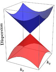
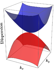
Figure 2: Schematic dispersion of (a) an isotropic Dirac semimetal (e.g., a single valley of graphene), and (b) a semi-Dirac semimetal exhibiting anisotropy.

IV Thermoelectric response for 2D nodal phases assuming constant relaxation time

In this section, we will demonstrate the computation of the transport coefficients for some 2D semimetals having nodal-points where two bands cross and consider the scenario when the relaxation time $\tau$ can be approximated to be a constant. We therefore set $d=2$ in the integrals derived in Sec. II and label the two-dimensional space by the Cartesian coordinates $x$ and $y$. In our notation, $1\Leftrightarrow x$ and $2\Leftrightarrow y$ for the Cartesian components of the vectors and tensors. Here we consider a single valley of graphene as an example of the isotropic dispersion case [cf. Fig. 2(a)], and the anisotropic Weyl (also known as semi-Dirac) semimetal as an example of the anisotropic dispersion scenario [cf. Fig. 2(b)].

IV.1 Isotropic case: a single valley of graphene

In this subsection, we compute the response matrix for graphene, which is a 2D isotropic Dirac semimetal. The low-energy Hamiltonian describing a single valley is given by [77]

$$H_{D}(k_{x},k_{y})=\hbar\,v\left(k_{x}\,\sigma_{x}+k_{y}\,\sigma_{y}\right),$$ (44)

where $\{\sigma_{x},\sigma_{y},\sigma_{z}\}$ are the three Pauli matrices, $\{k_{x},k_{y}\}$ are the momenta along the $x$ and $y$ directions, respectively, and $v$ is the Fermi velocity.

It is convenient to switch to the polar coordinate parametrization $k_{x}=k\,\cos\theta$ and $k_{y}=k\,\sin\theta$ (with $k\equiv|\mathbf{k}|\,$), such that the energy eigenvalues are given by $\epsilon_{\pm}({\bf k})=\pm\,\hbar\,v\,k$. The density of states (DOS) is given by

$$\rho_{g}(\epsilon)=\frac{|\epsilon|}{2\,\pi\,\hbar^{2}v^{2}}\,.$$ (45)

Using Eq. (II) along with an energy and momentum independent scattering time $\tau$, we get

$$\sigma_{\alpha\alpha}=\mathcal{L}_{\alpha\alpha}^{(0)}=\frac{\beta\,v^{2}\,e^{2}\,\tau}{8\,\pi\,\hbar^{2}}\int_{0}^{\infty}dk\,k\left[\text{sech}^{2}\left(\frac{\beta\left(k+\mu\right)}{2}\right)+\text{sech}^{2}\left(\frac{\beta\left(k-\mu\right)}{2}\right)\right]=\frac{e^{2}\,v^{2}\,\tau\,\ln\left(2+2\,\cosh\left(\beta\,\mu\right)\right)}{4\,\pi\,\hbar^{2}\,\beta}\,,$$ (46)

$$L_{\alpha\alpha}^{21}=\frac{-\mathcal{L}_{\alpha\alpha}^{(1)}}{e}$$

$$=\frac{\beta\,v^{2}\,e\,\tau}{8\,\pi^{2}\,\hbar^{2}}\int_{0}^{\infty}dk\,k\Big{[}\mu\left\{\text{sech}^{2}\left(\frac{\beta\left(k+\mu\right)}{2}\right)+\text{sech}^{2}\left(\frac{\beta\left(k-\mu\right)}{2}\right)\right\}+k\,\left\{\text{sech}^{2}\left(\frac{\beta\left(k+\mu\right)}{2}\right)-\text{sech}^{2}\left(\frac{\beta\left(k-\mu\right)}{2}\right)\right\}\Big{]}$$

$$=-\frac{v^{2}\,e\,\tau}{\left(2\,\beta\,\pi\,\hbar\right)^{2}}\left[\beta\,\mu\,\ln\left(2+2\,\cosh\left(\beta\,\mu\right)\right)+2\,{\text{Li}}_{2}(-e^{\beta\,\mu})-2\,{\text{Li}}_{2}(-e^{-\beta\,\mu})\right],$$ (47)

$$T\,L_{\alpha\alpha}^{22}=\frac{\mathcal{L}_{\alpha\alpha}^{(2)}}{e^{2}}$$

$$=\frac{\beta\,v^{2}\,\tau}{8\,\pi\,\hbar^{2}}\int_{0}^{\infty}dk\,k\,\Big{[}\text{sech}^{2}\left(\frac{\beta\left(k+\mu\right)}{2}\right)\left(k\,\epsilon_{0}+\mu\right)^{2}+\text{sech}^{2}\left(\frac{\beta\left(k-\mu\right)}{2}\right)\left(k-\mu\right)^{2}\Big{]}$$

$$=\frac{v^{2}\,\tau}{4\,\pi\,\hbar^{2}}\Big{[}\frac{4\,\mu\left\{{\text{Li}}_{2}(-e^{-\beta\,\mu})-{\text{Li}}_{2}(-e^{\beta\,\mu})\right\}}{\beta}+\frac{6\,{\text{Li}}_{3}(-e^{\beta\,\mu})+6\,{\text{Li}}_{3}(-e^{-\beta\,\mu})}{\beta^{2}}-\mu^{2}\,\ln\left(2+2\,\cosh\left(\beta\,\mu\right)\right)\Big{]}\,,$$ (48)

where

$$\text{Li}_{\chi}(z)=\sum\limits_{\ell=1}^{\infty}\frac{z^{\ell}}{\ell^{\chi}}$$ (49)

denotes the polylogarithm function of order $\chi$. At low temperatures [i.e., $\mu/(k_{B}T)\gg 1)$], the above results reduce to $\sigma_{\alpha\alpha}=e^{2}v^{2}\tau\mu/(4\pi\hbar^{2})$, and

$$L_{\alpha\alpha}^{21}=\frac{v^{2}\,e\,\tau}{4\,\pi\,\hbar^{2}}\times\frac{\pi^{2}\,(k_{B}\,T)^{2}}{3}\,,$$

$$T\,L_{\alpha\alpha}^{22}=\frac{v^{2}\,\tau}{4\,\pi\,\hbar^{2}}\times\frac{\mu\,\pi^{2}\,(k_{B}\,T)^{2}}{3}\,.$$ (50)

With these expressions, the Seebeck coefficients ($S$) at low temperature are found to be

$$S_{xx}=\frac{L_{xx}^{21}}{T\sigma_{xx}}\simeq-\frac{k_{B}\,T}{3\,e\,\mu}\text{ and }S_{yy}=\frac{L_{yy}^{21}}{T\sigma_{yy}}\simeq-\frac{k_{B}\,T}{3\,e\,\mu}\,.$$ (51)

Similarly, we obtain thermal conductivity to be

$$\kappa_{xx}=\kappa_{yy}=\frac{v^{2}\,e\,\tau}{4\,\pi\,\hbar^{2}T}\left[\frac{\pi^{2}\,\mu\,(k_{B}\,T)^{2}}{3}-\frac{3\,\pi^{4}\,(k_{B}\,T)^{3}}{9\,\mu}\right].$$ (52)

The longitudinal components of the thermal conductivity show linear-in-temperature dependence for both the $x$- and the $y$-axes.

IV.2 Anisotropic case: semi-Dirac semimetal

We consider a model of a 2D anisotropic semi-Dirac semimetal, with the Hamiltonian [29, 30, 31]

$$H_{\rm{semiD}}(k_{x},k_{y})=\frac{\hbar^{2}\,k_{x}^{2}}{2\,m}\,\sigma_{x}+\hbar\,v\,k_{y}\,\sigma_{y},$$ (53)

where $m$ is the effective mass along the $x$-axis and $v$ is the Fermi velocity along the $y$-axis. We will use $a=\frac{\hbar^{2}}{2\,m}$ and $b=\hbar\,v$ in the equations for simplifying the expressions. With these notations, the dispersion resulting from Eq. (53) is found to be $\epsilon_{\pm}({\mathbf{k}})=\pm\sqrt{a^{2}\,k_{x}^{4}+b^{2}\,k_{y}^{2}}$. This anisotropic nature of the spectrum invariably manifests itself in the transport coefficients for the system, which have been computed in Ref. [38] by following the methods outlined in Ref. [78]. We review those calculations and results in the remainder of this subsection.

With the parametrization $k_{x}=\text{sign}[\cos\theta]\left(\frac{{\tilde{r}}\,|\cos\theta|}{a}\right)^{1/2}$ and $k_{y}=\frac{{\tilde{r}}\,\sin\theta}{b}$ for ${\tilde{r}}\geq 0$, the energy eigenvalues take the simple form $\epsilon_{\pm}({\bf k})=\pm\,{\tilde{r}}$. The Jacobian of this transformation is given by

$$\mathcal{J}({\tilde{r}},\theta)=\left|\det\begin{pmatrix}\partial_{\tilde{r}}k_{x}&\partial_{\theta}k_{x}\vspace{0.2 cm}\\ \partial_{\tilde{r}}k_{y}&\partial_{\theta}k_{y}\end{pmatrix}\right|$$

$$=\begin{vmatrix}\frac{1}{2}\left(\frac{|\cos\theta|}{a\,{\tilde{r}}}\right)^{1/2}\vspace{0.2 cm}&-\frac{\sin\theta}{2}\left(\frac{{\tilde{r}}}{a\,|\cos\theta|}\right)^{1/2}\\ \sin\theta&{\tilde{r}}\cos\theta\end{vmatrix}$$

$$=\sqrt{\frac{{\tilde{r}}}{4\,a\,b^{2}\,|\cos\theta|}}\,.$$ (54)

Let us apply this convenient parametrization for calculating the DOS at energy $\epsilon>0$, which is given by

$$\rho_{sd}(\epsilon) =\int\frac{d^{2}\mathbf{k}}{\left(2\,\pi\right)^{2}}\,\delta\big{(}\epsilon-\epsilon_{+}({\bf k})\big{)}$$

$$=\int_{0}^{\infty}d\tilde{r}\int_{0}^{2\,\pi}\frac{d\theta}{\left(2\,\pi\right)^{2}}\,\mathcal{J}({\tilde{r}},\theta)\,\delta\big{(}\epsilon-{\tilde{r}}\big{)}$$

$$=\int_{0}^{2\,\pi}\frac{d\theta}{\left(2\,\pi\right)^{2}}\sqrt{\frac{\epsilon}{4\,a\,b^{2}\,|\cos\theta|}}=\frac{10.4882}{8\,\pi^{2}}\sqrt{\frac{\epsilon}{a\,b^{2}}}\,.$$ (55)

Clearly, the DOS of the semi-Dirac semimetal differs from its isotropic counterpart graphene featuring $\rho_{g}(\epsilon)\sim|\epsilon|$. The effects of the anisotropic dispersion will show up both via the characteristic DOS as well as the different values of the components of the Fermi velocity along the two mutually perpendicular directions.

Using Eq. (II) along with an energy and momentum independent scattering time $\tau$, we get

$$\sigma_{xx} =\mathcal{L}_{xx}^{(0)}=\frac{e^{2}\,\tau\,\sqrt{a}\,\beta}{8\,\pi^{2}\,\hbar^{2}\,b}\int_{0}^{\infty}d\tilde{r}\int_{0}^{2\,\pi}d\theta\,{\tilde{r}}^{3/2}\,|\cos\theta|^{5/2}\left[\text{sech}^{2}\left(\frac{\beta\left({\tilde{r}}-\mu\right)}{2}\right)+\text{sech}^{2}\left(\frac{\beta\left({\tilde{r}}+\mu\right)}{2}\right)\right]$$

$$=-\frac{2.16\,e^{2}\,\tau\sqrt{a}}{2\,\hbar^{2}\,b\,(\pi\,\beta)^{3/2}}\left[\text{Li}_{3/2}(-e^{\beta\,\mu)})+\text{Li}_{3/2}(-e^{-\beta\,\mu)})\right],$$ (56)

$$\sigma_{yy} =\mathcal{L}_{yy}^{(0)}=\frac{e^{2}\,\tau\,b\,\beta}{32\,\pi^{2}\,\hbar^{2}\,\sqrt{a}}\int_{0}^{\infty}d{\tilde{r}}\int_{0}^{2\,\pi}d\theta\,\sqrt{{\tilde{r}}\,|\sec\theta|}\,\sin^{2}\theta\left[\text{sech}^{2}\left(\frac{\beta\left({\tilde{r}}-\mu\right)}{2}\right)+\text{sech}^{2}\left(\frac{\beta\left({\tilde{r}}+\mu\right)}{2}\right)\right]$$

$$=-\frac{3.5\,e^{2}\,\tau\,b}{8\,\pi^{3/2}\,\hbar^{2}\,\sqrt{a\,\beta}}\left[\text{Li}_{1/2}(-e^{\beta\,\mu})+\text{Li}_{1/2}(-e^{-\beta\,\mu})\right].$$ (57)

For $\mu/(k_{B}\,T)\gg 1$, the above expressions reduce to

$$\sigma_{xx}=\frac{2.88\,e^{2}\,\tau\,\sqrt{a}}{2\,\pi^{2}\,\hbar^{2}\,b}\left[\mu^{3/2}+\frac{\pi^{2}\,(k_{B}\,T)^{2}}{8\,\sqrt{\mu}}\right],$$

$$\sigma_{yy}=\frac{7\,e^{2}\,\tau\,b}{8\,\pi^{2}\,\hbar^{2}\,\sqrt{a}}\left[\sqrt{\mu}-\frac{\pi^{2}\,(k_{B}\,T)^{2}}{24\,\mu^{3/2}}\right].$$ (58)

Evidently, the low-temperature longitudinal dc conductivities are direction-dependent, as expected from the fact that the components of the group velocity differ in the $x$- and $y$-directions. This is in contrast with the isotropic case (e.g., a single valley of graphene), where we have $\sigma_{xx}=\sigma_{yy}\sim\mu$.

The thermoelectric coefficients are obtained in a similar fashion as shown below:

$$L_{xx}^{21} =\frac{e\,\tau\,\sqrt{a}\,\beta}{8\,\pi^{2}\,\hbar^{2}\,b}\int_{0}^{\infty}d{\tilde{r}}\int_{0}^{2\,\pi}d\theta\,{\tilde{r}}^{3/2}\,|\cos\theta|^{5/2}\Bigg{[}\mu\left\{\text{sech}^{2}\left(\frac{\beta\left({\tilde{r}}+\mu\right)}{2}\right)+\text{sech}^{2}\left(\frac{\beta\left({\tilde{r}}-\mu\right)}{2}\right)\right\}$$

$$\hskip 199.16928pt+{\tilde{r}}\left\{\text{sech}^{2}\left(\frac{\beta\left({\tilde{r}}+\mu\right)}{2}\right)-\text{sech}^{2}\left(\frac{\beta\left({\tilde{r}}-\mu\right)}{2}\right)\right\}\Bigg{]}$$

$$=-\frac{2.16\,e\,\tau\,\sqrt{a}}{2\hbar^{2}\,b\,(\pi\,\beta)^{3/2}}\left[\mu\left\{\text{Li}_{3/2}(-e^{-\beta\,\mu)})+\text{Li}_{3/2}(-e^{\beta\,\mu)})\right\}+\frac{5}{2\,\beta}\left\{\text{Li}_{5/2}(-e^{-\beta\,\mu)})-\text{Li}_{5/2}(-e^{\beta\,\mu)})\right\}\right],$$ (59)

$$L_{yy}^{21} =\frac{e\,\tau\,b\,\beta}{32\,\pi^{2}\,\hbar^{2}\,\sqrt{a}}\int_{0}^{\infty}d{\tilde{r}}\int_{0}^{2\,\pi}d\theta\,\sqrt{{\tilde{r}}\,|\sec\theta|}\,\sin^{2}\theta\Bigg{[}\mu\left\{\text{sech}^{2}\left(\frac{\beta\left({\tilde{r}}+\mu\right)}{2}\right)+\text{sech}^{2}\left(\frac{\beta\left({\tilde{r}}-\mu\right)}{2}\right)\right\}$$

$$\hskip 241.84842pt+{\tilde{r}}\left\{\text{sech}^{2}\left(\frac{\beta\left({\tilde{r}}+\mu\right)}{2}\right)-\text{sech}^{2}\left(\frac{\beta\left({\tilde{r}}-\mu\right)}{2}\right)\right\}\Bigg{]}$$

$$=-\frac{3.5\,e\,\tau\,b}{8\,\pi^{3/2}\,\hbar^{2}\,\sqrt{a\,\beta}}\left[\mu\left\{\text{Li}_{1/2}(-e^{-\beta\,\mu)})+\text{Li}_{1/2}(-e^{\beta\,\mu)})\right\}+\frac{3}{2\,\beta}\left\{\text{Li}_{3/2}(-e^{-\beta\,\mu)})-\text{Li}_{3/2}(-e^{\beta\,\mu)})\right\}\right],$$ (60)

At low temperatures [i.e., $\mu/(k_{B}\,T)\gg 1$], we obtain

$$\L_{xx}^{21}=-\frac{2.88\,e\,\tau\,\sqrt{a}}{2\,\pi^{2}\,\hbar^{2}\,b}\left[\frac{\pi^{2}\,\mu^{1/2}}{2}(k_{B}\,T)^{2}\right],$$

$$\L_{yy}^{21}=-\frac{7\,e\,\tau\,b}{8\,\pi^{2}\,\hbar^{2}\,\sqrt{a}}\left[\frac{\pi^{2}}{6\,\mu^{1/2}}(k_{B}\,T)^{2}\right].$$ (61)

As before, the low-temperature behavior of the off-diagonal longitudinal thermal coefficients has an interesting direction dependence on the chemical potential. In contrast, the behaviour $L_{xx}^{21}=L_{yy}^{21}\sim(k_{B}\,T)^{2}$ [cf. Eq. (IV.1)] for graphene is independent of chemical potential. Although the individual coefficients in the semi-Dirac semimetal differ from those in graphene, the Mott relation still prevails at low temperature as seen from

$$S_{xx}=\frac{L_{xx}^{21}}{T\sigma_{xx}}\simeq-\frac{k_{B}\,T}{2\,e\,\mu}\text{ and }S_{yy}=\frac{L_{yy}^{21}}{T\sigma_{yy}}\simeq-\frac{k_{B}\,T}{6\,e\,\mu}\,.$$ (62)

These results show that at low-temeperatures and for momentum-independent relaxation time, there is no violation of the usual Mott relation. However, as will be evident in Sec. V, a momentum-dependent relaxation time may lead to deviation [79] from the linear-in-temperature dependence of the Mott relations.

To investigate electronic contribution to the thermal conductivity $\kappa$, we next compute

$$T\,L_{xx}^{22} =\frac{\mathcal{L}_{xx}^{(2)}}{e^{2}}$$

$$=\frac{\tau\sqrt{a}\,\beta}{8\,\pi^{2}\,\hbar^{2}\,b}\int_{0}^{\infty}d{\tilde{r}}\int_{0}^{2\,\pi}d\theta\,{\tilde{r}}^{3/2}\,|\cos\theta|^{5/2}\Big{[}\text{sech}^{2}\left(\frac{\beta\left({\tilde{r}}+\mu\right)}{2}\right)\left({\tilde{r}}+\mu\right)^{2}+\text{sech}^{2}\left(\frac{\beta\left({\tilde{r}}-\mu\right)}{2}\right)\left({\tilde{r}}-\mu\right)^{2}\Big{]}$$

$$=-\frac{2.16\,\tau\,\sqrt{a}}{2\,\hbar^{2}\,b\,(\pi\,\beta)^{3/2}}\Big{[}\mu^{2}\left\{\text{Li}_{3/2}(-e^{-\beta\,\mu)})+\text{Li}_{3/2}(-e^{\beta\,\mu)})\right\}+\frac{5\,\mu}{\beta}\left\{\text{Li}_{5/2}(-e^{-\beta\,\mu)})-\text{Li}_{5/2}(-e^{\beta\,\mu)})\right\}$$

$$\hskip 105.2751pt+\frac{35}{4\,\beta^{2}}\left\{\text{Li}_{7/2}(-e^{-\beta\,\mu)})+\text{Li}_{7/2}(-e^{\beta\,\mu)})\right\}\Big{]}$$ (63)

and

$$T\,L_{yy}^{22} =\frac{\mathcal{L}_{yy}^{(2)}}{e^{2}}$$

$$=\frac{\tau\,b\,\beta}{32\,\pi^{2}\,\hbar^{2}\,\sqrt{a}}\int_{0}^{\infty}d{\tilde{r}}\int_{0}^{2\,\pi}d\theta\,\sqrt{{\tilde{r}}\,|\sec\theta|}\sin^{2}\theta\Big{[}\text{sech}^{2}\left(\frac{\beta\left({\tilde{r}}+\mu\right)}{2}\right)\left({\tilde{r}}+\mu\right)^{2}+\text{sech}^{2}\left(\frac{\beta\left({\tilde{r}}-\mu\right)}{2}\right)\left({\tilde{r}}-\mu\right)^{2}\Big{]}$$

$$=-\frac{3.5\,e^{2}\,\tau\,b}{8\,\pi^{3/2}\hbar^{2}\,\sqrt{a\,\beta}}\Big{[}\mu^{2}\left\{\text{Li}_{1/2}(-e^{-\beta\,\mu)})+\text{Li}_{1/2}(-e^{\beta\,\mu)})\right\}+\frac{3\,\mu}{\beta}\left\{\text{Li}_{3/2}(-e^{-\beta\,\mu)})-\text{Li}_{3/2}(-e^{\beta\,\mu)})\right\}$$

$$\hskip 105.2751pt+\frac{15}{4\,\beta^{2}}\left\{\text{Li}_{5/2}(-e^{-\beta\,\mu)})+\text{Li}_{5/2}(-e^{\beta\,\mu)})\right\}\Big{]}.$$ (64)

At low temperatures [i.e., $\mu/(k_{B}\,T)\gg 1$], we obtain

$$T\,L_{xx}^{22} =\frac{2.88\,\tau\,\sqrt{a}}{2\,\pi^{2}\,\hbar^{2}\,b}\ \left[\frac{\pi^{2}\,\mu^{3/2}}{3}(k_{B}\,T)^{2}+\frac{7\,\pi^{4}}{40\,\mu^{1/2}}(k_{B}\,T)^{4}\right],$$

$$T\,L_{yy}^{22} =\frac{7\,\tau\,b}{8\,\pi^{2}\,\hbar^{2}\,\sqrt{a}}\left[\frac{\pi^{2}\,\mu^{1/2}}{3}(k_{B}\,T)^{2}-\frac{7\,\pi^{4}}{120\,\mu^{3/2}}(k_{B}\,T)^{4}\right].$$ (65)

Together with Eqs. (65) and (58), we recover the Wiedemann-Franz law, $L_{\alpha\alpha}^{22}=\frac{\pi^{2}\,k_{B}^{2}\,T}{3\,e^{2}}\sigma_{\alpha\alpha}$, up to leading order in $(k_{B}\,T)$. Finally, using Eq. (II), we get

$$\kappa_{xx}=\frac{2.88\,\tau\sqrt{a}}{2\,\pi^{2}\,\hbar^{2}\,b\,T}\left[\frac{\pi^{2}\,\mu^{3/2}\,(k_{B}\,T)^{2}}{3}-\frac{3\,\pi^{4}\,(k_{B}\,T)^{3}}{40\,\mu^{1/2}}\right],$$

$$\kappa_{yy}=\frac{7\,\tau b}{8\,\pi^{2}\,\hbar^{2}\,\sqrt{a}\,T}\left[\frac{\pi^{2}\mu^{1/2}\,(k_{B}\,T)^{2}}{3}-\frac{31\,\pi^{4}\,(k_{B}\,T)^{3}}{360\,\mu^{3/2}}\right].$$ (66)

As expected, the longitudinal components of the thermal conductivity show linear-in-temperature dependence for both the $x$- and the $y$-axes. However, their chemical potential dependence differs by a factor of $\mu$ (i.e., $\kappa_{xx}/\kappa_{yy}\sim\mu$) as a result of the inherent anisotropic nature of the Hamiltonian. We note that we have neglected phonon contribution to the thermal conductivity for simplicity. For strong contribution from phonon may lead to violation of the Wiedemann-Franz law.

Let us also investigate the form of the response in the opposite limit of $\mu/(k_{B}\,T)\ll 1$. In this high temperature limit, we get

$$\sigma_{xx}\simeq\frac{2.16\,e^{2}\,\tau\sqrt{a}}{2\,\hbar^{2}\,b\,(\pi\,\beta)^{3/2}}\left(1.5303+\frac{0.3801\,\mu^{2}}{k_{B}^{2}\,T^{2}}\right),$$

$$\sigma_{yy}\simeq\frac{3.5\,e^{2}\,\tau\,b}{8\,\pi^{3/2}\hbar^{2}\,\sqrt{a\,\beta}}\left(1.2098+\frac{0.1187\,\mu^{2}}{k_{B}^{2}\,T^{2}}\right),$$

$$L_{xx}^{21}=-\frac{2.16\,e^{2}\,\tau\sqrt{a}}{2\,\hbar^{2}\,b\,(\pi\,\beta)^{3/2}}\times 2.3\,\mu\,,$$

$$L_{yy}^{21}=-\frac{3.5\,e^{2}\,\tau\,b}{8\,\pi^{3/2}\hbar^{2}\,\sqrt{a\,\beta}}\times 0.60\,\mu\,,$$

$$L_{xx}^{22}=\frac{2.16\,e^{2}\,\tau\sqrt{a}\,\beta^{2}}{2\,T\,\hbar^{2}\,b\,(\pi\,\beta)^{3/2}}\left(16.88+\frac{0.6\,\mu^{2}}{k_{B}^{2}\,T^{2}}\right),$$

$$L_{yy}^{22}=\frac{3.5\,e^{2}\,\tau\,b\,\beta^{2}}{8\,\pi^{3/2}\,\hbar^{2}\,\sqrt{a\,\beta}}\left(6.54-\frac{0.15\,\mu^{2}}{k_{B}^{2}\,T^{2}}\,\right).$$ (67)

It turns out that the prefactors of both Eq. (IV.2) and Eq. (IV.2) give rise to dominant leading order contribution at high temperatures. Thus both $\sigma_{xx}$ and $L^{21}_{xx}$ go as $T^{3/2}$. Consequently, we obtain thermopower decaying with temperature. This is contrast with an isotropic dispersion, where the leading order behaviour turns out be $\sigma_{xx}\sim T$ and $L^{21}_{xx}\sim T^{2}$. This leads to a temperature-independent thermopower for graphene in the high-temperature regime [79].

V Thermoelectric response for 2D cases with short-ranged impurity scatterings

In this section, we consider the thermoelectric response, caused by scatterings due to short-ranged disorder, for both the graphene and semi-Dirac semimetal cases [38]. However, this kind of impurities is not very realistic for nodal semimetals because the relatively poor screening of charged impurities usually leads to longer-ranged interactions. Nevertheless, it is useful to investigate the predictions for the thermal properties of gapless isotropic and anisotropic Dirac materials . The short-ranged random disorder potential can be modelled by

$$V(\mathbf{r})=V_{0}\sum_{i}\delta(\mathbf{r}-\mathbf{r}_{i})\,,$$ (68)

where $\mathbf{r}_{i}$ and $V_{0}$ denote the random locations and the magnitude of the impurities, respectively. The scattering time, denoted by $\tau_{\rm{dis}}$, for such a disorder potential can be obtained from the Fermi’s golden rule as follows:

$$\frac{\hbar}{\tau_{\rm{dis}}}=2\pi\int\frac{d{\bf k^{\prime}}^{2}}{(2\pi)^{2}}\delta(\epsilon({\bf k})-\epsilon({\bf k^{\prime}}))V_{\bf k,k^{\prime}}^{2},$$ (69)

where $V_{\bf k,\bf k^{\prime}}=\langle{\bf k}|V|{\bf k^{\prime}}\rangle$ is the scattering matrix elements.

For graphene, using the expression above, we find

$$\tau_{\rm{dis}}=\frac{\hbar}{\pi\,V_{0}^{2}\,n_{\rm imp}\,\rho_{g}(\epsilon)}\,,$$ (70)

where $n_{\rm imp}$ is the impurity concentration. Thus, Eq. (45) tells us that $\tau_{\rm{dis}}\sim 1/\epsilon$, resulting in the thermopower to be exponentially suppressed at low temperatures [79], which is clearly seen from the expressions

$$S_{xx}=S_{yy}=-\mu\,\frac{e^{-\beta\,\mu}}{e\,T}\,.$$ (71)

In contrast, the scattering time for the short-ranged impurity in the semi-Dirac semi-metal is found to have angular dependence due to anisotropic dispersion [35]:

$$\tau_{\rm dis}=\frac{\tau_{0}(\epsilon)}{1+0.435\cos\theta}\,,$$ (72)

where $\tau_{0}(\epsilon)=\frac{\hbar}{\pi\,V_{0}^{2}\,n_{\rm imp}\,\rho_{sd}(\epsilon)}$. Considering the above energy dependence of the scattering rate (i.e., $\tau\sim 1/{\sqrt{\epsilon}}\,$), the transport coefficients at low temperatures [i.e., $\mu/({k_{B}T})\gg 1$] are found to be

$$\sigma_{xx}\simeq\frac{2.88\,e^{2}\tau\sqrt{a}}{2\,\pi^{2}\,\hbar^{2}\,b}\,\mu\,,~{}~{}~{}~{}\sigma_{yy}\simeq\frac{7\,e^{2}\,\tau\,b}{8\,\pi^{2}\,\hbar^{2}\,\sqrt{a}}\,,$$

$$L_{xx}^{21}\simeq-\frac{2.88\,e\,\tau\,\sqrt{a}}{2\,\pi^{2}\,\hbar^{2}\,b}\,\frac{(\pi\,k_{B}\,T)^{2}}{3},\quad L_{yy}^{21}\simeq-\frac{7\,e\,\tau\,b}{8\,\pi^{2}\,\hbar^{2}\sqrt{a}}\,\mu\,.$$ (73)

Evidently, the thermopower $S_{xx}$ follows the Mott relation, whereas $S_{yy}$ turns out to be independent of temperature (up to leading order).

VI Thermoelectric response for 2D cases with scatterings caused by charged impurities

Presence of charged impurities in a material acts as dopants, thus shifting the Fermi level away from the nodal-points. The screened Coulomb potential generated by such impurities is given by

$$V(q)=\frac{4\,\pi\,e^{2}}{q+q_{\text{\tiny}{\rm TF}}},$$ (74)

where $q_{\rm TF}$ is the Thomas-Fermi wavevector. The relaxation time within the Born approximation is then given by

$$\frac{1}{\tau(\epsilon(\mathbf{k}))} =\frac{2\,\pi\,n_{imp}}{\hbar}$$

$$\quad\times\sum\limits_{s=\pm}\int\frac{d^{2}\mathbf{k}^{\prime}}{(2\,\pi)^{2}}\,V^{2}(|\mathbf{k}-\mathbf{k}^{\prime}|)\,F_{\bf k\,k^{\prime}}\,\delta\big{(}\epsilon(\mathbf{k})-\epsilon_{s}(\mathbf{k}^{\prime})\big{)}\,,$$ (75)

where $F_{\bf k\,k^{\prime}}=\frac{1-\cos^{2}\phi_{\mathbf{k}\mathbf{k}^{\prime}}}{2}$, $\phi_{\mathbf{k}\mathbf{k}^{\prime}}$ is the angle between $\mathbf{k}$ and $\mathbf{k}^{\prime}$, and $n_{imp}$ is the impurity density.

For graphene, the screening has an important temperature dependence which in turns affects the thermopower. In fact, the temperature-dependent screening produces thermopower quadratic in temperature different from the Mott formula. In contrast, for unscreened charged impurity $\tau$ can be easily computed as $\tau\simeq\epsilon$. This in turn leads to thermopower linear in $T$ [79].

For the semi-Dirac semimetal, we use the parametrization introduced before, which leads to

$$\cos\phi_{\mathbf{k}\mathbf{k}^{\prime}}$$

$$=\frac{s_{0}\,\sqrt{\alpha\,|\cos\theta|}\,\sqrt{\alpha\,|\cos\theta^{\prime}|}+\sqrt{{\tilde{r}}\,{\tilde{r}}^{\prime}}\sin\theta\sin\theta^{\prime}}{\sqrt{\alpha\,|\cos\theta|+{\tilde{r}}\,\sin^{2}\theta}\,\sqrt{\alpha\,|\cos\theta^{\prime}|+{\tilde{r}}^{\prime}\sin^{2}\theta^{\prime}}}\,,$$ (76)

where $\alpha=b^{2}/a$, $s_{0}=\text{sign}[\cos\theta]\,\text{sign}[\cos\theta^{\prime}]$, and ${\tilde{r}}^{\prime}\geq 0$. For definiteness, let us consider the case when $s=+$. Since $\epsilon_{\mathbf{k}}^{+}={\tilde{r}}$ is independent of $\theta$, we set $\theta=\frac{\pi}{2}$ without any loss of generality. This leads to

$$F_{\bf k,k^{\prime}}=\frac{\alpha\,|\cos(\theta^{\prime})|}{2\,(\,|\cos\theta^{\prime}|+{\tilde{r}}^{\prime}\sin^{2}\theta^{\prime}\,)}\,.$$ (77)

Together with Eq. (77), (75) and (IV.2), we obtain

$$\frac{1}{\tau({\tilde{r}})} =\frac{4\,\pi\,n_{imp}\,e^{4}\,\alpha}{\hbar\,{\tilde{r}}^{3/2}}$$

$$\quad\times\int\frac{d\theta^{\prime}\,\sqrt{\alpha\,|\cos\theta^{\prime}|}}{\left[(1-\sin\theta^{\prime})^{2}+\frac{\alpha\,|\cos\theta^{\prime}|}{{\tilde{r}}}\right]\left(\alpha\,|\cos\theta^{\prime}|+{\tilde{r}}\sin^{2}\theta^{\prime}\right)}\,,$$ (78)

where we have considered $q_{\rm{TF}}=0$ for unscreened charge impurities. In this case, Eq. (78) can be further simplified in the various limits as follows (assuming $\alpha\sim 1$):

$$\frac{1}{\tau({\tilde{r}})}\simeq\frac{4\,\pi\,e^{4}\,n_{imp}}{\hbar}\begin{cases}\frac{8.0}{{\tilde{r}}}&\text{ for }{\tilde{r}}\ll 1\\ &\\ \frac{6.0476}{{\tilde{r}}^{5/3}}+\frac{16.509}{{\tilde{r}}^{7/3}}-\frac{10.6889}{{\tilde{r}}^{3}}&\text{ for }{\tilde{r}}\gg 1\end{cases}.$$ (79)

The first limit is found from the leading order contribution of $2\int_{-\pi/2+{\tilde{r}}}^{\pi/2-{\tilde{r}}}\frac{d\theta^{\prime}\,\sqrt{|\cos\theta^{\prime}|}}{\left(\frac{|\cos\theta^{\prime}|}{{\tilde{r}}}\right)\left(|\cos\theta^{\prime}|\right)}$, whereas the second limit is found from the leading order contribution of $4\int_{0}^{\pi/2-\left({4}/{{\tilde{r}}}\right)^{1/3}}\frac{d\theta^{\prime}\,\sqrt{|\cos\theta^{\prime}|}}{\left(1-\sin\theta^{\prime}\right)^{2}\,{\tilde{r}}\,\sin^{2}\theta^{\prime}}$.

We emphasize that the scattering from the unscreened Coulomb interaction in graphene is known to be $\tau\sim\epsilon$ irrespective of the values of $\epsilon$. In contrast, the anisotropy in Eq. (53) leads to a different expression for energy-dependent scattering for $\epsilon\gg 1$. Considering the leading energy dependent term for $\tau\sim\epsilon^{5/3}$, we find that

$$\sigma_{xx}=\frac{2.88\,e^{2}\,\tau\,\sqrt{a}}{2\,\pi^{2}\,\hbar^{2}\,b}\left[\mu^{19/6}+\frac{247\,\mu^{7/6}\,\pi^{2}}{216}\,(k_{B}\,T)^{2}\right],$$

$$\sigma_{yy}=\frac{7\,e^{2}\,\tau\,b}{8\,\pi^{2}\,\hbar^{2}\,\sqrt{a}}\left[\mu^{13/6}+\frac{91\,\mu^{1/6}\,\pi^{2}}{216}(k_{B}\,T)^{2}\right],$$

$$L_{xx}^{21}=-\frac{2.88\,e\,\tau\,\sqrt{a}}{2\,\pi^{2}\,\hbar^{2}\,b}\times\frac{19\,\pi^{2}\mu^{13/6}(k_{B}\,T)^{2}}{18},$$

$$L_{yy}^{21}=-\frac{7\,e\,\tau\,b}{8\,\pi^{2}\,\hbar^{2}\,\sqrt{a}}\times\frac{13\,\pi^{2}\,\mu^{7/6}(k_{B}\,T)^{2}}{18}\,.$$ (80)

Thus we recover the Mott relation of $S_{\alpha\alpha}\sim T$. However, the dc conductivities exhibit dependence on the chemical potential due to the energy-dependent relaxation time.

VII Thermopower for 2D cases in presence of a weak magnetic field

Having discussed the thermoelectric properties without any external magnetic field, we next turn to the thermopower for finite magnetic field $\mathbf{B}=B\,\hat{z}$ in presence of a finite $\partial_{x}T$ ( but $\mathbf{E}$ set to zero), focussing on the case of a semi-Dirac semimetal. Assuming the solution $\delta f_{n}$ independent of time due to the static $\mathbf{B}$ field, the linearized form of Boltzmann equation [cf. Eq. (14)] is found to be

$$\frac{e\,B}{\hbar\,c}\left(v_{x}\,\partial_{k_{y}}-v_{y}\,\partial_{k_{x}}\right)\delta f_{n}+v_{x}\left(\epsilon_{n}-\mu\right)\partial_{x}T\,\frac{\partial f_{n}^{(0)}}{\partial\epsilon_{n}}$$

$$=-\delta f_{n}/\tau.$$ (81)

Following Ref. [5, 7], the appropriate ansatz for $\delta f_{n}$ leads to the thermoelectric coefficients as

$$L_{\alpha\beta}^{11}=-\int d\epsilon\,\frac{\partial f^{(0)}(\epsilon)}{\partial\epsilon}\,\tilde{\sigma}_{\alpha\beta}(\epsilon)\,,$$

$$L_{\alpha\beta}^{21}=-e\int d\epsilon\,\frac{\partial f^{(0)}(\epsilon)}{\partial\epsilon}\,(\epsilon-\mu)\,\tilde{\sigma}_{\alpha\beta}(\epsilon)\,,$$ (82)

where the energy-dependent $\tilde{\sigma}_{\alpha\beta}(\epsilon)$’s are the components of the matrix

$$\tilde{\sigma}(\epsilon) =\sigma_{0}(\epsilon)\begin{pmatrix}v_{x}^{2}(\epsilon)&-B\,\tau\,\tilde{v}_{x}(\epsilon)\cr B\,\tau\,\tilde{v}_{y}(\epsilon)&v_{y}^{2}(\epsilon)\end{pmatrix},$$

$$\sigma_{0}(\epsilon) =e^{2}\,\rho_{sd}(\epsilon)\,\tau\,,\quad v_{x}^{2}(\epsilon)={2.88\,a\,\epsilon}/{\pi^{2}}\,,\quad v_{y}^{2}(\epsilon)=7\,b^{2}\,,$$

$$\tilde{v}_{x}(\epsilon) =v_{x}^{2}(\epsilon)\,\,\partial^{2}_{k_{y}}\epsilon-v_{x}(\epsilon)\,v_{y}(\epsilon)\,\partial_{k_{x}}\partial_{k_{y}}\epsilon\,,$$

$$\tilde{v}_{y}(\epsilon) =v_{y}^{2}(\epsilon)\,\,{\partial_{k_{x}}^{2}\epsilon}-v_{x}(\epsilon)\,v_{y}(\epsilon)\,\,\partial_{k_{x}}\partial_{k_{y}}\epsilon\,.$$ (83)

We note that the diagonal elements of $\sigma(\epsilon)$ are taken up to zeroth-order in $B$ and, for off-diagonal components, we retain the leading order terms in $B$. For simplicity, we assume $\tau$ to be independent of the energy. For $k_{B}\,T\ll\mu$ and $\hbar\,\omega_{c}\ll\mu$, Eq. (VII) can be further simplified as

$$L_{\alpha\beta}^{11}\simeq\tilde{\sigma}_{\alpha\beta}(\mu)\,,\quad L_{\alpha\beta}^{21}\simeq\frac{\pi^{2}\left(k_{B}\,T\right)^{2}}{3\,e}\frac{d\tilde{\sigma}_{\alpha\beta}(\epsilon)}{d\epsilon}\Bigg{|}_{\epsilon=\mu}\,.$$ (84)

These allow us to compute the longitudinal components of the thermopower, which take the following forms:

$$S_{xx} \simeq\frac{\pi^{2}\,k_{B}^{2}\,T}{3\,e\,\mu}$$

$$\,\times\frac{1.5\,v^{2}_{x}(\epsilon)\,v^{2}_{y}(\epsilon)+B^{2}\,\tau^{2}\,\tilde{v}_{x}(\epsilon)\left[0.5\,\tilde{v}_{y}(\epsilon)+\mu\,\partial_{\epsilon}\tilde{v}_{y}(\epsilon)\right]}{v^{2}_{x}(\epsilon)\,v^{2}_{y}(\epsilon)+B^{2}\,\tau^{2}\,\tilde{v}^{2}_{x}(\epsilon)\,\tilde{v}^{2}_{y}(\epsilon)}\Bigg{|}_{\epsilon=\mu},$$

$$S_{yy} \simeq\frac{\pi^{2}\,k_{B}^{2}\,T}{3\,e}$$

$$\,\times\frac{\frac{0.5\,v^{2}_{x}(\epsilon)\,v^{2}_{y}(\epsilon)}{\mu}+B^{2}\,\tau^{2}\,\tilde{v}_{y}(\epsilon)\left[0.5\,\tilde{v}_{x}(\epsilon)+\mu\,\partial_{\epsilon}\tilde{v}_{x}(\epsilon)\right]}{v^{2}_{x}(\epsilon)\,v^{2}_{y}(\epsilon)+B^{2}\,\tau^{2}\,\tilde{v}^{2}_{x}(\epsilon)\,\tilde{v}^{2}_{y}(\epsilon)}\Bigg{|}_{\epsilon=\mu}.$$ (85)

Evidently, in the limit of $B\rightarrow 0$, these expressions coincide with those shown in Eq. (51).

VIII Thermopower for 2D cases in presence of a strong magnetic field

In this section, we take the same set-up as considered in Sec. VII, but elucidate the characteristics of the thermopower in presence of a quantizing (i.e., strong) magnetic field along the $z$-direction such that Landau levels are formed. Our strategy is to use the entropy ($\mathcal{S}$) in determining the thermopower. We observe that since the heat current is the electronic contribution to the heat transport in an electronic system, the Seebeck coefficient can be expressed in terms of the entropy of the system. We motivate this strategy by considering the case of a one-dimensional wire oriented along the $x$-direction, which then deals with the case of the longitudinal Seebeck coefficient $S_{xx}$ only. An electrostatic potential gradient ($\delta V$) appears on applying a temperature gradient, such that $\delta V=S_{xx}\,\partial_{x}T$. Using thermodynamics, we have the relation $n_{0}\,e\,\delta V\sim S\,\delta T$, where $n_{0}$ is the number density of the carriers, which in turn gives $S_{xx}={\mathcal{S}}/\left(e\,n_{0}\right)$.

In order to derive the explicit relation between the entropy and the Seebeck coefficient in the presence of sufficiently strong magnetic field, we begin with the general expression of thermoelectric coefficients $L^{12}_{xy}$ and $L^{11}_{xy}$ [81] given by

$$L^{11}_{xy}=-\frac{e^{2}}{h}\sum_{l}\int_{\epsilon_{l}-\mu}^{\infty}d\epsilon\,{\partial f^{(0)}(\epsilon)\over\partial\epsilon}\,,$$

$$L^{12}_{xy}=\frac{k_{B}\,e\,\beta}{h}\sum_{l}\int_{\epsilon_{l}-\mu}^{\infty}d\epsilon\,\epsilon\,{\partial f^{(0)}(\epsilon)\over\partial\epsilon}\,,$$ (86)

where $\epsilon_{l}$ here denotes the Landau level energies and $f^{(0)}(\epsilon)={1}/\left(1+e^{\beta\,\epsilon}\right)$ [cf. Eq. (9)]. We would like to point out that the macroscopic transport properties are independent of the specific details of the confining potential in the sample, although the microscopic currents do depend on it. Eq. (VIII) can be further simplified by changing variables from $\epsilon\rightarrow f^{(0)}$, leading to [1, 2]

$$L^{11}_{xy} =-\frac{e^{2}}{h}\sum_{l}f_{l}\,,$$

$$L^{12}_{xy} =\frac{k_{B}\,e}{h}\sum_{l}\int_{\epsilon_{l}-\mu}^{\infty}\,f_{l}\,\left[\ln(1-f_{l})-\ln f_{l}\right]$$

$$=\frac{e\,\mathcal{S}}{h}\,.$$ (87)

Here, $f_{l}=f^{(0)}(\epsilon_{l}-\mu)$ and

$$\mathcal{S}=-k_{B}\sum_{l}\left[\,f_{l}\ln f_{l}+(1-f_{l})\ln(1-f_{l})\,\right]$$ (88)

is the total entropy of the carriers. This leads to the form $S_{xx}={\mathcal{S}}/\left(e\,n_{0}\right)$ for the longitudinal thermopower.

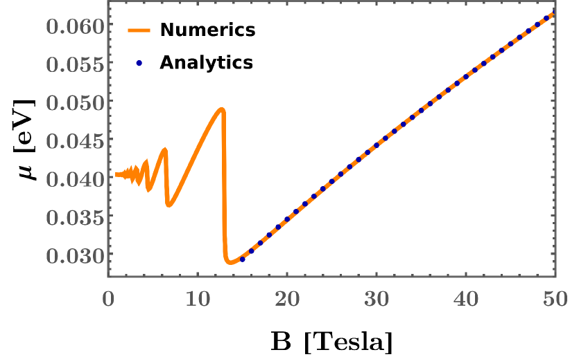
Figure 3: Plot (solid orange line) of the chemical potential as a function of the strength of the magnetic field for electron density $n_{0}=5\times 10^{11}$ cm^-2 at temperature $T=5$ K. The behaviour in the strong field regime represented by the blue dots is obtained from the approximate analytical form shown in Eq. (93), using the values $b_{0}=0.0017$ eV, $b_{1}=0.0006$ eV Tesla^-2/3, $b_{2}=0.0014$ eV, and $b_{3}=1$ Tesla^-1 as the fitting parameters. Considering parameter values characteristic of Dirac semimetals, we have used $v=5\times 10^{5}$ m/s and $m=3.1\times m_{e}$, where $m_{e}$ is the electron mass.

For a semi-Dirac semimetal, in the presence of a quantizing magnetic magnetic field $\mathbf{B}=B\,\hat{\mathbf{z}}$ [using the Landau gauge $\boldsymbol{A}=(-B\,y,0,0)$], the energy of the Landau levels are found to be [39]

$$\epsilon_{l}= \pm 1.17325\left(m\,v^{2}\right)^{1/3}\left[\left(l+1/2\right)\hbar\,\omega_{c}\right]^{2/3}$$

$$\text{with }l\in\{0,{\mathbb{Z}}^{+}\}\,,$$ (89)

where $\omega_{c}={e\,B}/{m}$ is the effective cyclotron frequency. With this, we obtain

$$S_{xx}=\frac{k_{B}}{2\,\pi\,n_{0}\,e\,l_{b}^{2}}\sum_{l}\left[\ln(1+e^{\tilde{x}_{l}})-\frac{{\tilde{x}_{l}}\,e^{\tilde{x}_{l}}}{e^{\tilde{x}_{l}}+1}\right],$$ (90)

where $\tilde{x}_{l}=\beta\,(\epsilon_{l}-\mu)$, $l_{b}=\sqrt{\frac{\hbar}{e\,B}}$ is the magnetic length, $n_{0}$ fixes the Fermi energy through

$$n_{0}=2\times\frac{1}{2\,\pi\,l_{b}^{2}}\sum_{l=0}^{\infty}f_{l}\Big{|}_{\epsilon_{l}>0}\,,$$ (91)

with the factor of $2$ accounting for the contributions coming from $\epsilon_{l}<0$.

For a reasonably strong magnetic field [i.e., for $\hbar\,\omega_{c}\gg\mu$], the system enters into a strong quantum limit and the quasiparticles occupy only the $l=0$ Landau levels. In this regime, we can approximate Eq. (91) as:

$$n_{0}\simeq\,\frac{1}{\pi\,l_{b}^{2}}\times\frac{1}{1+e^{\beta\,\left(|\epsilon_{0}|-\mu\right)}}\,.$$ (92)

This leads to $\mu=|\epsilon_{0}|-\beta^{-1}\ln(\frac{1}{n_{0}\,\pi\,\l_{b}^{2}}-1)$, with the leading-order field dependence captured by

$$\mu=b_{0}+b_{1}\,B^{2/3}+b_{2}\ln(b_{3}\,B-1)\,,$$ (93)

where $\{b_{0},\,b_{1},\,b_{2},\,b_{3}\}$ can be readily obtained from the approximate anaytical solution of $\mu$. This approximate analytical result fits reasonably well with the numerical solution obtained from Eq. (92), as corroborated by the curves in Fig. 3, which confirms it validity. Notably, Eq. (93) differs from the 3D version (which is also known as the double-Weyl semimetal) exhibiting $\mu\sim{B}^{-1}$. This difference of course originates from the specific magnetic field dependence of the Landau level spectrum. We note that for weak enough values of the magnetic field strength, which refers to the limit $\hbar\,\omega_{c}\ll\mu$, the chemical potential is mostly unaffected by the magnetic field. As we increase the stength of the magnetic field, we start to observe quantum oscillations in the chemical potential, which in turn leads to oscillations in the thermopower as well.

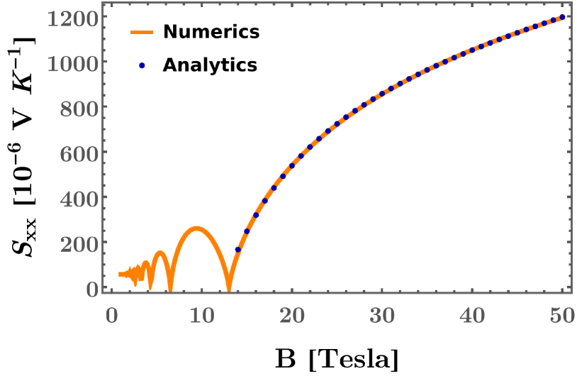
Figure 4: Plot (solid orange line) of $S_{xx}$, as shown in Eq. (90), as a function of the strength of the magnetic field for an electron density of $n_{0}=5\times 10^{11}\,\rm{cm}^{-2}$ at temperature $T=5$ K. The blue dots represent the approximate analytical results obtained using Eq. (94). The values of the parameters $v$ and $m$ are the same as in Fig. 3.

In order to find the approximate high field dependence of the thermopower, we plug in the expression for $\mu$ [given by Eq. (93)] into Eq. (90) after setting $l=0$. This results in

$$S_{xx} =\frac{k_{B}}{e}\left[\left(\pi\,n_{0}\,l_{b}^{2}\right)\ln\left(1-\pi\,n_{0}\,l_{b}^{2}\right)-\ln\left(\frac{1}{\pi\,n_{0}\,l_{b}^{2}}-1\right)\right]$$

$$=\frac{k_{B}}{e}\left[\left(1-\frac{B}{\alpha_{0}}\right)\ln\left(1-\frac{\alpha_{0}}{B}\right)-\ln\left(\frac{\alpha_{0}}{B}\right)\right],$$

$$\alpha_{0} =\frac{n_{0}\,h}{2\,e}\,.$$ (94)

In order to verify this complex $B$-dependence in our analytical approximation, we numerically evaluate Eq. (90) using the numerical solution of $\mu(B)$. Fig. 4 shows the behaviour of $S_{xx}$ as a function of $B$. Clearly, the approximate large field dependence of $S_{xx}$ (represented by the blue dots), obtained from the formula shown above, fits well with the numerical solution (shown by the solid orange line) of Eq. (90). Interestingly, the part of the thermopower curve obtained in the low-field region also agrees very well with the experimental results available for $\alpha$-(BEDT-TTF)₂I₃ [82].

In contrast to the semi-Dirac case, the Landau levels in graphene take the form

$$\epsilon_{l}\propto\begin{cases}\pm\,\sqrt{l}&\text{for }l>0\\ 0&\text{for }l=0\end{cases}\,,$$ (95)

showing a square root dependence on $l\in{\mathbb{Z}}$. Subsequently, the Seebeck coefficients are found to oscillate at low temperature as functions of the Landau level index $l$ for a fixed magnetic field [83]. Moreover, $S_{xx}$ has been found to increase slowly as a function of magnetic field [84]. For the 3D Dirac and Weyl nodes, the Landau levels disperse in one of the momentum directions. This in turn leads to a strong field dependence $S_{xx}$ which varies as $S_{xx}\sim B^{2}$ [9].

Finally, we comment on the behaviour of the transverse thermoelectric coefficient $S_{xy}$, also dubbed as the magneto-thermoelectric Nernst-Ettinghausen effect. Using the relation $S_{xy}=L^{12}_{xy}/L_{xy}^{11}$, this can be found using Eq. (VIII). It turns out that $S_{xy}$ oscillates as a function of the chemical potential. The maximum value of $S_{xy}$ is given by $k_{B}\,e^{-1}\ln 2$, corroborating the universal behavior pointed out by in Ref. [81]. However, the peak positions differ from graphene or typical semiconductors. We again attribute this difference to the difference in the Landau spectrum, as discussed before.

IX Thermoelectric response for 3D Weyl semimetals in planar Hall and planar thermal Hall set-ups

Using the formalism reviewed in Sec. III, in this section, we show the expressions for the response related to PHE and PHNE for a single Weyl node with chirality $\chi$ (taking the values of $\pm$ 1), which is described by the Hamiltonian

$$H=\chi\,\hbar\,v_{F}\,\boldsymbol{\sigma}\cdot\mathbf{k},$$ (96)

where $v_{F}$ is the Fermi velocity and $\mathbf{k}$ is the 3D wavevector. In the following, we will use natural units, thus setting $\hbar$, $c$, and $k_{B}$ to unity. Furthermore, we will neglect the orbital magnetization of the Bloch wavepacket and consider the low temperature regime, satisfying $\beta\mu\gg 1$, such that Sommerfeld expression is applicable for evaluating the response involving integrands with functions of the Fermi-Dirac distribution function.

The eigenvalues of the Hamiltonian are given by

$$\epsilon_{n}({\mathbf{k}})=-(-1)^{n}\,v_{F}\,k\ \,,\quad n\in\{1,2\}\,,$$ (97)

where the value $1$($2$) for the band index $n$ refers to the conduction(valence) band.

The Berry curvature expression for the node is captured by

$$\mathbf{\Omega}_{\chi,n}({\mathbf{k}})=\frac{\chi\,(-1)^{n}}{2\,k^{3}}\left\{k_{x},\,k_{y},\,k_{z}\right\},$$ (98)

while the band velocity vector for the quasiparticles is given by

$${\boldsymbol{v}}_{n}(\mathbf{k})=\nabla_{\mathbf{k}}\,\epsilon_{n}({\mathbf{k}})=-\frac{(-1)^{n}\,v_{F}}{k}\left\{k_{x},\,k_{y},\,k_{z}\right\}.$$ (99)

Henceforth, we will consider the situation when the chemical potential cuts the conduction band such that the quasiparticles in that band participate in the trasport.

The longitudinal magnetoconductivity tensor [cf. Eq. (III)] evaluates to [73]

$$\bar{\sigma}_{xx}^{\chi} =\frac{\tau\,e^{2}\,\mu^{2}}{6\,\pi^{2}\,v_{F}}\left(1+\frac{\pi^{2}}{3\,\beta^{2}\,\mu^{2}}\right)$$

$$\qquad+\frac{\tau\,e^{4}\,v_{F}^{3}\left(8\,B_{x}^{2}+B_{y}^{2}\right)}{64\,\pi^{\frac{3}{2}}\,\mu^{2}\,\Gamma(\frac{7}{2})}\left(1+\frac{\pi^{2}}{\beta^{2}\,\mu^{2}}\right).$$ (100)

The first term in $\bar{\sigma}_{xx}^{\chi}$ is independent of the magnetic field and has a nonzero value even at zero temperature. This $\mathbf{B}$-independent part is usually referred to as the Drude contribution. The planar Hall conductivity tensor [cf. Eq. (III)] takes the form [73]

$$\bar{\sigma}_{yx}^{\chi}=\bar{\sigma}_{xy}^{\chi}=\frac{7\,\tau\,e^{4}\,v_{F}^{3}\,B_{x}\,B_{y}}{64\,\pi^{\frac{3}{2}}\,\mu^{2}\,\Gamma(\frac{7}{2})}\left(1+\frac{\pi^{2}}{\beta^{2}\,\mu^{2}}\right).$$ (101)

The expression for the longitudinal thermoelectric coefficient [cf. Eq. (III)] turns out to be [73]

$$\bar{L}_{xx}^{12}=-\frac{\tau\,e\,\mu}{9\,v_{F}\,\beta}+\frac{\tau\,e^{3}\,v_{F}^{3}\,{\sqrt{\pi}}\,\mu^{-3}}{96\,\beta\,\Gamma(\frac{7}{2})}\left(8\,B_{x}^{2}+B_{y}^{2}\right).$$ (102)

Comparing with Eq. (IX), we observe that $\partial_{\mu}\bar{\sigma}_{xx}^{\chi}=-\frac{3\,e\,\beta}{\pi^{2}}\,\bar{L}_{xx}^{12}+\mathcal{O}(\beta^{-2})$. Hence, the Mott relation $L_{\alpha\gamma}^{12}=-\frac{\pi^{2}}{3\,e\,\beta}\,\partial_{\mu}L_{\alpha\gamma}^{11}$, which holds in the $\beta\rightarrow\infty$ limit, is satisfied [85]. Finally, the expression for the longitudinal thermoelectric coefficient [cf. Eq. (III)] is found to be [73]

$$\bar{L}_{yx}^{12}=\bar{L}_{xy}^{12}=\frac{7\,\tau\,e^{3}\,v_{F}^{3}\,{\sqrt{\pi}}\,\mu^{-3}\,B_{x}\,B_{y}}{96\,\beta\,\Gamma(\frac{7}{2})}\,.$$ (103)

Comparing with Eq. (101), we observe that $\partial_{\mu}\bar{\sigma}_{yx}^{\chi}=-\frac{3\,e\,\beta}{\pi^{2}}\,\bar{L}_{yx}^{12}+\mathcal{O}(\beta^{-2})$. Therefore, in this case too, we find that the Mott relation $L_{\alpha\gamma}^{12}=-\frac{\pi^{2}}{3\,e\,\beta}\,\partial_{\mu}L_{\alpha\gamma}^{11}$ (valid in the $\beta\rightarrow\infty$ limit) is satisfied [85].

The planar Hall response results from the nontrivial Berry phase and chiral anomaly, which is manifested by a negative magnetoresistance, a quadratic-in-magnetic-field dependence of the magnetoconductance, and an oscillatory behaviour with the angle $\theta$ between the electric and the magnetic fields. These are seen in the theoretical expressions eludcidated above and corroborate the data obtained in numerous experiments. A few examples of such experiments involve materials like ZrTe₅ [86], TaAs [87], NbP and NbAs [61], and Co₃Sn₂S₂ [88], hosting Weyl nodes in their bandstructures.

X Summary and outlook

In this review, we have presented the methods to compute the thermoelectric coefficients in nodal-point semimetals, covering bothe 2D and 3D cases.

In 2D, we have provided the explicit expressions of the response tensors taking the specific examples of graphene and semi-Dirac semimetal, which represent the cases with isotropic and anisotropic dispersions, respectively. We have investigated these properties both in the absence and in the presence of an external magnetic field applied along the direction perpendicular to the plane of the semimetals. For the zero and weak (nonquantizing) magnetic field cases, we have employed the semiclassical Boltzmann formalism (along with a relation time approximation) to derive the expressions for the elements of the response matrix (built out of the thermoelectric transport coefficients). In order to demonstrate how the response depends on the primary mechanism responsible for the scatterings of the emergent quasiparticles under a given situation, in addition to the simplest case of a constant relaxation time, we have considered the appropriate forms of the relaxation time arising due to the influence of short-ranged disorder potential and screened charged impurities. In all the cases considered, we have showed that an anisotropy in the band-spectrum invariably affects the response quite significantly. We have illustrated this point by comparing the results for a semi-Dirac semimetal with those for the graphene. Some of these observations include the following:

1. In the low-temperature regime, the components of the dc conductivity tensor for a semi-Dirac semimetal have a different dependence on the chemical potential (or Fermi level) compared to the case of graphene.

2. In the high-temperature limits, the thermoelectric response decays with temperature in the semi-Dirac semimetal. On the contrary, the response is independent of temperature in graphene.

3. The relaxation rates due to short-ranged impurity potential and screened Coulomb interaction caused by charged impurities lead to distinct expressions for the dc and thermal conductivities.

4. For the strong magnetic field case, when we need to consider the Landau levels, we have outlined a procedure to compute the response using the entropy of the carriers. Using the formula derived through this pathway, we have illustrated the results for the response via numerical data, in addition to providing analytical approximations. While the thermopower shows a strong unsaturating behaviour for the semi-Dirac semimetal [cf. Fig. 4], $S_{xx}$ in graphene increases with $B$ at a much slower rate.

The results for various distinct cases, as summarized above, prove beyond doubt that the interplay of anisotropy and strengths of externally applied electromagnetic fields might lead to useful technological applications like achieving a high value of thermoelectric figure-of-merit [1].

For the 3D nodal phases, we have shown the explicit expressions for the various conductivity tensors, applicable in planar Hall and planar thermal Hall set-ups, considering a Weyl semimetal node. Such expressions for anisotropic nodal-point semimetals are available in the literature [68, 11, 12, 73].

The results presented here can also be easily generalized to the case of multiple nodes and band-crossings involving more than two bands (e.g., 2D pseudospin-1 Dirac–Weyl semimetal [89] and 3D quadratic band-touching semimetal [90]). In presence of long-ranged Coulomb potential, the nodal-point semimemetals may transition into non-Fermi liquid phases when the Fermi level cuts a band-crossing point [91, 92, 93, 94], in which case the techniques discussed in this review will fail. The way out is to use strong-coupling techniques like (a) Kubo formula with the theory regulated using methods like large-N expansion and/or dimensional regularization [91, 92, 95, 96, 94]; or (b) memory-matrix approach [95, 97, 96]. Another possibility even in the presence of screened Coulomb interactions is the emergence of the plasmons depending on the parameter regime, which will then drastically affect the relaxation time [98, 99, 100], necessitating the use of quantum field theoretic methods to compute any transport characteristics. The full-fledged analysis of the effects of strong disorder on the transport properties is another aspect worthy of careful investigations, which also requires strong-coupling approaches [101, 102, 103, 104, 94]. The same applies for short-ranged strong interactions [105, 106].

References

- Skinner and Fu [2018] B. Skinner and L. Fu, Large, nonsaturating thermopower in a quantizing magnetic field, Science Advances 4, 2621 (2018).
- Bergman and Oganesyan [2010] D. L. Bergman and V. Oganesyan, Theory of dissipationless Nernst effects, Phys. Rev. Lett. 104, 066601 (2010).
- Wei et al. [2009a] P. Wei, W. Bao, Y. Pu, C. N. Lau, and J. Shi, Anomalous thermoelectric transport of Dirac particles in graphene, Phys. Rev. Lett. 102, 166808 (2009a).
- Zhu et al. [2010] L. Zhu, R. Ma, L. Sheng, M. Liu, and D.-N. Sheng, Universal thermoelectric effect of Dirac fermions in graphene, Phys. Rev. Lett. 104, 076804 (2010).
- Sharma et al. [2016] G. Sharma, P. Goswami, and S. Tewari, Nernst and magnetothermal conductivity in a lattice model of Weyl fermions, Phys. Rev. B 93, 035116 (2016).
- Sharma et al. [2017a] G. Sharma, C. Moore, S. Saha, and S. Tewari, Nernst effect in Dirac and inversion-asymmetric Weyl semimetals, Phys. Rev. B 96, 195119 (2017a).
- Lundgren et al. [2014a] R. Lundgren, P. Laurell, and G. A. Fiete, Thermoelectric properties of Weyl and Dirac semimetals, Phys. Rev. B 90, 165115 (2014a).
- Sharma et al. [2017b] G. Sharma, P. Goswami, and S. Tewari, Chiral anomaly and longitudinal magnetotransport in type-II Weyl semimetals, Phys. Rev. B 96, 045112 (2017b).
- Liang et al. [2017] T. Liang, J. Lin, Q. Gibson, T. Gao, M. Hirschberger, M. Liu, R. J. Cava, and N. P. Ong, Anomalous Nernst effect in the Dirac semimetal Cd3As2, Phys. Rev. Lett. 118, 136601 (2017).
- Chernodub et al. [2018] M. N. Chernodub, A. Cortijo, and M. A. H. Vozmediano, Generation of a Nernst current from the conformal anomaly in Dirac and Weyl semimetals, Phys. Rev. Lett. 120, 206601 (2018).
- Nag and Nandy [2021] T. Nag and S. Nandy, Magneto-transport phenomena of type-I multi-Weyl semimetals in co-planar setups, Journal of Physics Condensed Matter 33, 075504 (2021).
- Yadav et al. [2022] S. Yadav, S. Fazzini, and I. Mandal, Magneto-transport signatures in periodically-driven Weyl and multi-Weyl semimetals, Physica E Low-Dimensional Systems and Nanostructures 144, 115444 (2022).
- Mandal et al. [2020] D. Mandal, K. Das, and A. Agarwal, Magnus Nernst and thermal Hall effect, Phys. Rev. B 102, 205414 (2020).
- Papaj and Fu [2019] M. Papaj and L. Fu, Magnus Hall effect, Phys. Rev. Lett. 123, 216802 (2019).
- Sekh, Sajid and Mandal, Ipsita [2022] Sekh, Sajid and Mandal, Ipsita, Magnus Hall effect in three-dimensional topological semimetals, Eur. Phys. J. Plus 137, 736 (2022).
- Sbierski et al. [2014] B. Sbierski, G. Pohl, E. J. Bergholtz, and P. W. Brouwer, Quantum transport of disordered Weyl semimetals at the nodal point, Phys. Rev. Lett. 113, 026602 (2014).
- Huang et al. [2013] Z. Huang, D. P. Arovas, and A. V. Balatsky, Impurity scattering in Weyl semimetals and their stability classification, New Journal of Physics 15, 123019 (2013).
- Ominato and Koshino [2014] Y. Ominato and M. Koshino, Quantum transport in a three-dimensional Weyl electron system, Phys. Rev. B 89, 054202 (2014).
- Hosur et al. [2012] P. Hosur, S. A. Parameswaran, and A. Vishwanath, Charge transport in Weyl semimetals, Phys. Rev. Lett. 108, 046602 (2012).
- Landsteiner [2014] K. Landsteiner, Anomalous transport of Weyl fermions in Weyl semimetals, Phys. Rev. B 89, 075124 (2014).
- Fauqué et al. [2013] B. Fauqué, N. P. Butch, P. Syers, J. Paglione, S. Wiedmann, A. Collaudin, B. Grena, U. Zeitler, and K. Behnia, Magnetothermoelectric properties of Bi2Se3, Phys. Rev. B 87, 035133 (2013).
- Xiao et al. [2005] D. Xiao, J. Shi, and Q. Niu, Berry phase correction to electron density of states in solids, Phys. Rev. Lett. 95, 137204 (2005).
- Zhu et al. [2015] Z. Zhu, X. Lin, J. Liu, B. Fauqué, Q. Tao, C. Yang, Y. Shi, and K. Behnia, Quantum oscillations, thermoelectric coefficients, and the Fermi surface of semimetallic WTe2, Phys. Rev. Lett. 114, 176601 (2015).
- Ferreiros et al. [2017] Y. Ferreiros, A. A. Zyuzin, and J. H. Bardarson, Anomalous Nernst and thermal Hall effects in tilted Weyl semimetals, Phys. Rev. B 96, 115202 (2017).
- Gorbar et al. [2017] E. V. Gorbar, V. A. Miransky, I. A. Shovkovy, and P. O. Sukhachov, Anomalous thermoelectric phenomena in lattice models of multi-Weyl semimetals, Phys. Rev. B 96, 155138 (2017).
- McCormick et al. [2017] T. M. McCormick, R. C. McKay, and N. Trivedi, Semiclassical theory of anomalous transport in type-II topological Weyl semimetals, Phys. Rev. B 96, 235116 (2017).
- Stålhammar et al. [2020] M. Stålhammar, J. Larana-Aragon, J. Knolle, and E. J. Bergholtz, Magneto-optical conductivity in generic Weyl semimetals, Phys. Rev. B 102, 235134 (2020).
- Yadav et al. [2023] S. Yadav, S. Sekh, and I. Mandal, Magneto-optical conductivity in the type-I and type-II phases of Weyl/multi-Weyl semimetals, Physica B Condensed Matter 656, 414765 (2023).
- Pardo and Pickett [2009] V. Pardo and W. E. Pickett, Half-metallic semi-Dirac-point generated by quantum confinement in TiOVO2 nanostructures, Phys. Rev. Lett. 102, 166803 (2009).
- Pardo and Pickett [2010] V. Pardo and W. E. Pickett, Metal-insulator transition through a semi-Dirac point in oxide nanostructures: VO2 (001) layers confined within TiO2, Phys. Rev. B 81, 035111 (2010).
- Banerjee et al. [2009] S. Banerjee, R. R. P. Singh, V. Pardo, and W. E. Pickett, Tight-binding modeling and low-energy behavior of the semi-Dirac point, Phys. Rev. Lett. 103, 016402 (2009).
- Kobayashi et al. [2011] A. Kobayashi, Y. Suzumura, F. Piéchon, and G. Montambaux, Emergence of Dirac electron pair in the charge-ordered state of the organic conductor -(BEDT-TTF)2i3, Phys. Rev. B 84, 075450 (2011).
- Suzumura et al. [2013] Y. Suzumura, T. Morinari, and F. Piéchon, Mechanism of Dirac point in type organic conductor under pressure, Journal of the Physical Society of Japan 82, 023708 (2013).
- Hasegawa et al. [2006] Y. Hasegawa, R. Konno, H. Nakano, and M. Kohmoto, Zero modes of tight-binding electrons on the honeycomb lattice, Phys. Rev. B 74, 033413 (2006).
- Adroguer et al. [2016] P. Adroguer, D. Carpentier, G. Montambaux, and E. Orignac, Diffusion of Dirac fermions across a topological merging transition in two dimensions, Phys. Rev. B 93, 125113 (2016).
- Montambaux et al. [2009a] G. Montambaux, F. Piéchon, J.-N. Fuchs, and M. O. Goerbig, Merging of Dirac points in a two-dimensional crystal, Phys. Rev. B 80, 153412 (2009a).
- Montambaux et al. [2009b] G. Montambaux, F. Piéchon, J.-N. Fuchs, and M. O. Goerbig, A universal Hamiltonian for motion and merging of Dirac points in a two-dimensional crystal, The European Physical Journal B 72, 509 (2009b).
- Mandal and Saha [2020] I. Mandal and K. Saha, Thermopower in an anisotropic two-dimensional Weyl semimetal, Phys. Rev. B 101, 045101 (2020).
- Dietl et al. [2008] P. Dietl, F. Piéchon, and G. Montambaux, New magnetic field dependence of Landau levels in a graphenelike structure, Phys. Rev. Lett. 100, 236405 (2008).
- Cho and Moon [2016] G. Y. Cho and E.-G. Moon, Novel quantum criticality in two dimensional topological phase transitions, Scientific Reports 6, 19198 (2016).
- Chen and Fiete [2016a] Q. Chen and G. A. Fiete, Thermoelectric transport in double-Weyl semimetals, Phys. Rev. B 93, 155125 (2016a).
- Ashcroft and Mermin [2011] N. Ashcroft and N. Mermin, Solid State Physics (Cengage Learning, 2011).
- Tong [2012] D. Tong, Lectures on Kinetic Theory (2012).
- Arovas [2014] D. Arovas, Lecture Notes on Condensed Matter Physics (CreateSpace Independent Publishing Platform, 2014).
- Soto [2016] R. Soto, Kinetic Theory and Transport Phenomena, Oxford master series in condensed matter physics (Oxford University Press, 2016).
- Onsager [1931] L. Onsager, Reciprocal relations in irreversible processes. I., Phys. Rev. 37, 405 (1931).
- Nielsen and Ninomiya [1981] H. Nielsen and M. Ninomiya, A no-go theorem for regularizing chiral fermions, Physics Letters B 105, 219 (1981).
- Sundaram and Niu [1999] G. Sundaram and Q. Niu, Wave-packet dynamics in slowly perturbed crystals: Gradient corrections and Berry-phase effects, Phys. Rev. B 59, 14915 (1999).
- Son and Spivak [2013] D. T. Son and B. Z. Spivak, Chiral anomaly and classical negative magnetoresistance of Weyl metals, Phys. Rev. B 88, 104412 (2013).
- Xiao et al. [2010] D. Xiao, M.-C. Chang, and Q. Niu, Berry phase effects on electronic properties, Rev. Mod. Phys. 82, 1959 (2010).
- Duval et al. [2006] C. Duval, Z. Horváth, P. A. Horvathy, L. Martina, and P. Stichel, Berry phase correction to electron density in solids and “exotic” dynamics, Mod. Phys. Lett. B 20, 373 (2006).
- Son and Yamamoto [2012] D. T. Son and N. Yamamoto, Berry curvature, triangle anomalies, and the chiral magnetic effect in fermi liquids, Phys. Rev. Lett. 109, 181602 (2012).
- Lundgren et al. [2014b] R. Lundgren, P. Laurell, and G. A. Fiete, Thermoelectric properties of Weyl and Dirac semimetals, Phys. Rev. B 90, 165115 (2014b).
- Das and Agarwal [2019] K. Das and A. Agarwal, Linear magnetochiral transport in tilted type-I and type-II Weyl semimetals, Phys. Rev. B 99, 085405 (2019).
- Nandy et al. [2017] S. Nandy, G. Sharma, A. Taraphder, and S. Tewari, Chiral anomaly as the origin of the planar Hall effect in Weyl semimetals, Phys. Rev. Lett. 119, 176804 (2017).
- Nandy et al. [2019] S. Nandy, A. Taraphder, and S. Tewari, Planar thermal Hall effect in Weyl semimetals, Phys. Rev. B 100, 115139 (2019).
- Xiao and Niu [2020] C. Xiao and Q. Niu, Unified bulk semiclassical theory for intrinsic thermal transport and magnetization currents, Phys. Rev. B 101, 235430 (2020).
- Qin et al. [2011] T. Qin, Q. Niu, and J. Shi, Energy magnetization and the thermal Hall effect, Phys. Rev. Lett. 107, 236601 (2011).
- Zhang [2016] L. Zhang, Berry curvature and various thermal Hall effects, New Journal of Physics 18, 103039 (2016).
- Burkov [2017] A. A. Burkov, Giant planar Hall effect in topological metals, Phys. Rev. B 96, 041110 (2017).
- Li et al. [2017] Y. Li, Z. Wang, P. Li, X. Yang, Z. Shen, F. Sheng, X. Li, Y. Lu, Y. Zheng, and Z.-A. Xu, Negative magnetoresistance in Weyl semimetals NbAs and NbP: Intrinsic chiral anomaly and extrinsic effects, Frontiers of Physics 12, 127205 (2017).
- Nandy et al. [2018] S. Nandy, A. Taraphder, and S. Tewari, Berry phase theory of planar Hall effect in topological insulators, Scientific Reports 8, 14983 (2018).
- Zhang et al. [2016] S.-B. Zhang, H.-Z. Lu, and S.-Q. Shen, Linear magnetoconductivity in an intrinsic topological Weyl semimetal, New Journal of Physics 18, 053039 (2016).
- Chen and Fiete [2016b] Q. Chen and G. A. Fiete, Thermoelectric transport in double-Weyl semimetals, Phys. Rev. B 93, 155125 (2016b).
- Das and Agarwal [2020] K. Das and A. Agarwal, Thermal and gravitational chiral anomaly induced magneto-transport in Weyl semimetals, Phys. Rev. Res. 2, 013088 (2020).
- Das et al. [2022] S. Das, K. Das, and A. Agarwal, Nonlinear magnetoconductivity in Weyl and multi-Weyl semimetals in quantizing magnetic field, Phys. Rev. B 105, 235408 (2022).
- Pal et al. [2022a] O. Pal, B. Dey, and T. K. Ghosh, Berry curvature induced magnetotransport in 3d noncentrosymmetric metals, Journal of Physics: Condensed Matter 34, 025702 (2022a).
- Pal et al. [2022b] O. Pal, B. Dey, and T. K. Ghosh, Berry curvature induced anisotropic magnetotransport in a quadratic triple-component fermionic system, Journal of Physics: Condensed Matter 34, 155702 (2022b).
- Fu and Wang [2022] L. X. Fu and C. M. Wang, Thermoelectric transport of multi-Weyl semimetals in the quantum limit, Phys. Rev. B 105, 035201 (2022).
- Araki [2020] Y. Araki, Magnetic textures and dynamics in magnetic Weyl semimetals, Annalen der Physik 532, 1900287 (2020).
- Mizuta and Ishii [2014] Y. P. Mizuta and F. Ishii, Contribution of Berry curvature to thermoelectric effects, Proceedings of the International Conference on Strongly Correlated Electron Systems (SCES2013) 3, 017035 (2014).
- Medel Onofre and Martín-Ruiz [2023] L. Medel Onofre and A. Martín-Ruiz, Planar Hall effect in Weyl semimetals induced by pseudoelectromagnetic fields, Phys. Rev. B 108, 155132 (2023).
- Ghosh and Mandal [2023] R. Ghosh and I. Mandal, Electric and thermoelectric response for Weyl and multi-Weyl semimetals in planar Hall configurations including the effects of strain, arXiv e-prints (2023), arXiv:2310.02318 [cond-mat.mes-hall] .
- Haldane [2004] F. D. M. Haldane, Berry curvature on the Fermi surface: Anomalous Hall effect as a topological Fermi-liquid property, Phys. Rev. Lett. 93, 206602 (2004).
- Goswami and Tewari [2013] P. Goswami and S. Tewari, Axionic field theory of -dimensional Weyl semimetals, Phys. Rev. B 88, 245107 (2013).
- Burkov [2014] A. A. Burkov, Anomalous Hall effect in Weyl metals, Phys. Rev. Lett. 113, 187202 (2014).
- Slonczewski and Weiss [1958] J. C. Slonczewski and P. R. Weiss, Band structure of graphite, Phys. Rev. 109, 272 (1958).
- Park et al. [2017] S. Park, S. Woo, E. J. Mele, and H. Min, Semiclassical Boltzmann transport theory for multi-Weyl semimetals, Phys. Rev. B 95, 161113 (2017).
- Hwang et al. [2009] E. H. Hwang, E. Rossi, and S. Das Sarma, Theory of thermopower in two-dimensional graphene, Phys. Rev. B 80, 235415 (2009).
- Suh et al. [2023] J. Suh, S. Park, and H. Min, Semiclassical Boltzmann magnetotransport theory in anisotropic systems with a nonvanishing Berry curvature, New Journal of Physics 25, 033021 (2023).
- Girvin and Jonson [1982] S. M. Girvin and M. Jonson, Inversion layer thermopower in high magnetic field, Journal of Physics C: Solid State Physics 15, L1147 (1982).
- Konoike et al. [2013] T. Konoike, M. Sato, K. Uchida, and T. Osada, Anomalous thermoelectric transport and giant Nernst effect in multilayered massless Dirac fermion system, Journal of the Physical Society of Japan 82, 073601 (2013).
- Wei et al. [2009b] P. Wei, W. Bao, Y. Pu, C. N. Lau, and J. Shi, Anomalous thermoelectric transport of Dirac particles in graphene, Phys. Rev. Lett. 102, 166808 (2009b).
- Checkelsky and Ong [2009] J. G. Checkelsky and N. P. Ong, Thermopower and Nernst effect in graphene in a magnetic field, Phys. Rev. B 80, 081413 (2009).
- Xiao et al. [2006] D. Xiao, Y. Yao, Z. Fang, and Q. Niu, Berry-phase effect in anomalous thermoelectric transport, Phys. Rev. Lett. 97, 026603 (2006).
- Li et al. [2016] Q. Li, D. E. Kharzeev, C. Zhang, Y. Huang, I. Pletikosić, A. V. Fedorov, R. D. Zhong, J. A. Schneeloch, G. D. Gu, and T. Valla, Chiral magnetic effect in ZrTe5, Nature Physics 12, 550 (2016).
- Zhang et al. [2016] C.-L. Zhang, S.-Y. Xu, I. Belopolski, Z. Yuan, Z. Lin, B. Tong, G. Bian, N. Alidoust, C.-C. Lee, S.-M. Huang, T.-R. Chang, G. Chang, C.-H. Hsu, H.-T. Jeng, M. Neupane, D. S. Sanchez, H. Zheng, J. Wang, H. Lin, C. Zhang, H.-Z. Lu, S.-Q. Shen, T. Neupert, M. Zahid Hasan, and S. Jia, Signatures of the Adler-Bell-Jackiw chiral anomaly in a Weyl fermion semimetal, Nature Communications 7, 10735 (2016).
- Shama et al. [2020] Shama, R. Gopal, and Y. Singh, Observation of planar Hall effect in the ferromagnetic Weyl semimetal Co3Sn2S2, Journal of Magnetism and Magnetic Materials 502, 166547 (2020).
- Bradlyn et al. [2016] B. Bradlyn, J. Cano, Z. Wang, M. G. Vergniory, C. Felser, R. J. Cava, and B. A. Bernevig, Beyond Dirac and Weyl fermions: Unconventional quasiparticles in conventional crystals, Science 353, aaf5037 (2016).
- [90] A. A. Abrikosov and S. D. Beneslavskiĭ, Possible existence of substances intermediate between metals and dielectrics, in 30 Years of the Landau Institute — Selected Papers, pp. 64–73.
- Abrikosov [1974] A. A. Abrikosov, Calculation of critical indices for zero-gap semiconductors, Sov. Phys.-JETP 39, 709 (1974).
- Moon et al. [2013] E.-G. Moon, C. Xu, Y. B. Kim, and L. Balents, Non-Fermi-liquid and topological states with strong spin-orbit coupling, Phys. Rev. Lett. 111, 206401 (2013).
- Roy et al. [2017] B. Roy, P. Goswami, and V. Juričić, Interacting Weyl fermions: Phases, phase transitions, and global phase diagram, Phys. Rev. B 95, 201102 (2017).
- Mandal [2021] I. Mandal, Robust marginal Fermi liquid in birefringent semimetals, Physics Letters A 418, 127707 (2021).
- Mandal and Freire [2021] I. Mandal and H. Freire, Transport in the non-Fermi liquid phase of isotropic Luttinger semimetals, Phys. Rev. B 103, 195116 (2021).
- Mandal and Freire [2022] I. Mandal and H. Freire, Raman response and shear viscosity in the non-Fermi liquid phase of Luttinger semimetals, Journal of Physics Condensed Matter 34, 275604 (2022).
- Freire and Mandal [2021] H. Freire and I. Mandal, Thermoelectric and thermal properties of the weakly disordered non-Fermi liquid phase of Luttinger semimetals, Physics Letters A 407, 127470 (2021).
- Kozii and Fu [2018] V. Kozii and L. Fu, Thermal plasmon resonantly enhances electron scattering in Dirac/Weyl semimetals, Phys. Rev. B 98, 041109 (2018).
- Mandal [2019] I. Mandal, Search for plasmons in isotropic Luttinger semimetals, Annals of Physics 406, 173 (2019).
- Wang and Mandal [2023] J. Wang and I. Mandal, Anatomy of plasmons in generic Luttinger semimetals, arXiv e-prints , arXiv:2303.10163 (2023).
- Mandal and Ziegler [2021] I. Mandal and K. Ziegler, Robust quantum transport at particle-hole symmetry, EPL (Europhysics Letters) 135, 17001 (2021).
- Nandkishore and Parameswaran [2017] R. M. Nandkishore and S. A. Parameswaran, Disorder-driven destruction of a non-Fermi liquid semimetal studied by renormalization group analysis, Phys. Rev. B 95, 205106 (2017).
- Mandal and Nandkishore [2018] I. Mandal and R. M. Nandkishore, Interplay of Coulomb interactions and disorder in three-dimensional quadratic band crossings without time-reversal symmetry and with unequal masses for conduction and valence bands, Phys. Rev. B 97, 125121 (2018).
- Mandal [2018] I. Mandal, Fate of superconductivity in three-dimensional disordered Luttinger semimetals, Annals of Physics 392, 179 (2018).
- Avdoshkin et al. [2020] A. Avdoshkin, V. Kozii, and J. E. Moore, Interactions remove the quantization of the chiral photocurrent at Weyl points, Phys. Rev. Lett. 124, 196603 (2020).
- Mandal [2020] I. Mandal, Effect of interactions on the quantization of the chiral photocurrent for double-weyl semimetals, Symmetry 12 (2020).