Group Spike and Slab Variational Bayes

Abstract

We introduce Group Spike-and-slab Variational Bayes (GSVB), a scalable method for group sparse regression. A fast co-ordinate ascent variational inference (CAVI) algorithm is developed for several common model families including Gaussian, Binomial and Poisson. Theoretical guarantees for our proposed approach are provided by deriving contraction rates for the variational posterior in grouped linear regression. Through extensive numerical studies, we demonstrate that GSVB provides state-of-the-art performance, offering a computationally inexpensive substitute to MCMC, whilst performing comparably or better than existing MAP methods. Additionally, we analyze three real world datasets wherein we highlight the practical utility of our method, demonstrating that GSVB provides parsimonious models with excellent predictive performance, variable selection and uncertainty quantification.

Keywords: High-dimensional regression, Group sparsity, Generalized Linear Models, Sparse priors, Bayesian Methods

1 Introduction

Group structures arise in various applications, such as genetics (Wang et al., 2007; Breheny and Huang, 2009), imaging (Lee and Cao, 2021), multi-factor analysis of variance (Meier et al., 2008), non-parametric regression (Huang et al., 2010), and multi-task learning, among others. In these settings, $p$-dimensional feature vectors, $x_{i}=(x_{i1},\dots,x_{ip})^{\top}\in\mathbb{R}^{p}$, for $i=1,\dots,n$ observations can be partitioned into groups of features. Formally this means that we can construct sub-vectors, $x_{G_{k}}=\{x_{j}:j\in G_{k}\}$ for $k=1,\dots,M$, where the groups $G_{k}=\{G_{k,1},\dots,G_{k,m_{k}}\}$ are disjoint sets of indices satisfying $\bigcup_{k=1}^{M}G_{k}=\{1,\dots,p\}$. Typically, these group structures are known beforehand, for example in genetics where biological pathways (gene sets) are known, or they are constructed artificially, for example, through a basis expansion in non-parametric additive models.

In the regression setting incorporating these group structures is crucial, as disregarding them can result in sub-optimal models (Huang and Zhang, 2010; Lounici et al., 2011). In this manuscript, we focus on the general linear regression model (GLM) where, for each observation $i=1,\dots,n$, the response, $Y_{i}$ can be modelled by

$$\mathbb{E}[Y_{i}|x_{i},\beta]=f\left(\sum_{k=1}^{M}x_{i,G_{k}}^{\top}\beta_{G_{k}}\right),\quad i=1,\dots,n$$ (1)

where $f:\mathbb{R}\rightarrow\mathbb{R}$ represents the link function, $\beta=(\beta_{1},\dots,\beta_{p})^{\top}\in\mathbb{R}^{p}$ denotes the model coefficient vector with $\beta_{G_{k}}=\{\beta_{j}:j\in G_{k}\}$. Beyond incorporating the group structure, it is often of practical importance to identify the groups of features that are associated with the response. This holds particularly true when there are a large number of them. To address this, various methods have been proposed over the years, with one of the most popular being the group LASSO (Yuan and Lin, 2006), which applies an $\ell_{2,1}$ norm to groups of coefficients. Following Yuan and Lin (2006) there have been numerous extensions, including the group SCAD (Wang et al., 2007), the group LASSO for logistic regression (Meier et al., 2008), the group bridge (Huang et al., 2009), group LASSO with overlapping groups (Jacob et al., 2009), and the sparse group LASSO (Breheny and Huang, 2009; Simon et al., 2013), among others (see Huang et al. (2012) for a detailed review of frequentist methods).

In a similar vein, Bayesian group selection methods have arisen. The earliest of which being the Bayesian group LASSO (Raman et al., 2009; Kyung et al., 2010), which uses a multivariate double exponential distribution prior to impose shrinkage on groups of coefficients. Notably, the maximum a posteriori (MAP) estimate under this prior coincides with the estimate under the group LASSO. Other methods include Bayesian sparse group selection (Xu and Ghosh, 2015; Chen et al., 2016) and the group spike-and-slab LASSO (Bai et al., 2020) which approach the problem via stochastic search variable selection (Mitchell and Beauchamp, 1988; Chipman, 1996). Formally, these methods utilize a group spike-and-slab prior, a mixture distribution of a multivariate Dirac mass on zero and a continuous distribution over $\mathbb{R}^{m_{k}}$, where $m_{k}$ is the size of the $k$th group. Such priors have been shown to work excellently for variable selection as they are able to set coefficients exactly to zero, avoiding the use of shrinkage to enforce sparsity. For a comprehensive review see Lai and Chen (2021) and Jreich et al. (2022).

However, a serious drawback of these methods is that most use Markov Chain Monte Carlo (MCMC) to sample from the posterior (Raman et al., 2009; Xu and Ghosh, 2015; Chen et al., 2016). In general, MCMC approaches are known to be computationally expensive when there are a large number of variables, and within the group setting they can result in poor mixing when group sizes are large (Chen et al., 2016). To circumvent these issues, some authors proposed computing MAP estimates (Kyung et al., 2010; Bai et al., 2020), by relaxing the form of the prior, replacing the multivariate Dirac mass with a continuous distribution concentrated at zero (Ročková and George, 2018). Although these algorithms are fast to compute, they come at the sacrifice of interpretability, as posterior inclusion probabilities no longer guarantee the coefficient is zero but rather concentrated at zero. Beyond this, these algorithms only return a point estimate for $\beta$ and therefore do not provide uncertainty quantification – a task at the heart of Bayesian inference.

To bridge the gap between scalability and uncertainty quantification several authors have turned to variational inference (VI). An approach to inference wherein the posterior distribution is approximated by a tractable family of distributions known as the variational family (see Zhang et al. (2019) for a review). In the context of high-dimensional Bayesian inference, VI has proven particularly successful, and has been employed in linear regression (Carbonetto and Stephens, 2012; Ormerod et al., 2017; Ray and Szabó, 2022), logistic regression (Ray et al., 2020) and survival analysis (Komodromos et al., 2022) to name a few. Within the context of Bayesian group regression, to our knowledge only the Bayesian group LASSO has seen a variational counterpart (Babacan et al., 2014).

In this manuscript we examine the variational Bayes (VB) posterior arising from the group spike-and-slab prior with multivariate double exponential slab and Dirac spike, referring to our method as Group Spike-and-slab Variational Bayes (GSVB). We provide scalable variational approximations to three common classes of generalized linear models: the Gaussian with identity link function, Binomial with logistic link function, and Poisson with exponential link function. We outline a general scheme for computing the variational posterior via co-ordinate ascent variational inference. We further show that for specific cases, the variational family can be re-parameterized to allow for more efficient updates.

Through extensive numerical experiments we demonstrate that GSVB achieves state-of-the-art performance while significantly reducing computation time by several orders of magnitude compared to MCMC. Moreover, through our comparison with MCMC, we highlight that the variational posterior provides excellent uncertainty quantification through marginal credible sets with impressive coverage. Additionally, the proposed method is compared against the spike-and-slab group LASSO (Bai et al., 2020), a state-of-the-art Bayesian group selection algorithm that returns MAP estimates. Within this comparison our method demonstrates comparable or better performance in terms of group selection and effect estimation, whilst carrying the added benefit of providing uncertainty quantification, a feature not available by other scalable methods in the literature.

To highlight the practical utility of our method, we analyse three real datasets, demonstrating that our method provides excellent predictive accuracy, while also achieving parsimonious models. Additionally, we illustrate the usefulness of the VB posterior by showing its ability to provide posterior predictive intervals, a feature not available to methods that provide MAP estimates, and computationally prohibitive to compute via MCMC.

Theoretical guarantees for our method are provided in the form of posterior contraction rates, which quantify how far the posterior places most of its probability from the ‘ground truth’ generating the data for large sample sizes. This approach builds on the work of Castillo et al. (2015) and Ray and Szabó (2022), and extends previous Bayesian contraction rate results for true posteriors in the group sparse setting (Ning et al., 2020; Bai et al., 2020) to their variational approximation.

Concurrent to our work, Lin et al. (2023) proposed a similar spike-and-slab model for group variable selection in linear regression, which appeared on arXiv shortly after our preprint.

Notation. Let $y=(y_{1},\dots,y_{n})^{\top}\in\mathbb{R}^{n}$ denote the realization of the random vector $Y=(Y_{1},\dots,Y_{n})$. Further, let $X=(x_{1},\dots,x_{n})^{\top}\in\mathbb{R}^{n\times p}$ denote the design matrix, where for a group $G_{k}$ let $X_{G_{k}}=(x_{1,G_{k}},\dots,x_{n,G_{k}})^{\top}\in\mathbb{R}^{n\times m_{k}}$. Similarly, for $G_{k}^{c}=\{1,\dots,p\}\setminus G_{k}$, denote $X_{G_{k}^{c}}=(x_{1,G_{k}^{c}},\dots,x_{n,G_{k}^{c}})^{\top}\in\mathbb{R}^{n\times(p-m_{k})}$ where $x_{i,G_{k}^{c}}=\{x_{ij}:j\in G_{k}^{c}\}$, and $\beta_{G_{k}^{c}}=\{\beta_{j}:j\in G_{k}^{c}\}$. Wherein, without loss of generality we assume that the elements of the groups are ordered such that $1=G_{1,1}<G_{1,2}<\dots<G_{M,m_{M}}=p$. Finally, the Kullback-Leibler divergence is defined as $D_{\text{KL}}=D_{\text{KL}}(Q\|P)=\int_{\mathcal{X}}\log\left(\frac{dQ}{dP}\right)dQ$, where $Q$ and $P$ are probability measures on $\mathcal{X}$, such that $Q$ is absolutely continuous with respect to $P$.

2 Prior and Variational family

To model the coefficients $\beta$, we consider a group spike-and-slab prior. For each group $G_{k}$, the prior over $\beta_{G_{k}}$ consists of a mixture distribution of a multivariate Dirac mass on zero and a multivariate double exponential distribution, $\Psi(\beta_{G_{k}})$, whose density is given by,

$$\psi(\beta_{G_{k}};\lambda)=C_{k}\lambda^{m_{k}}\exp\left(-\lambda\|\beta_{G_{k}}\|\right)$$

where $C_{k}=[2^{m_{k}}\pi^{(m_{k}-1)/2}\Gamma((m_{k}+1)/2)]^{-1}$ and $\|\cdot\|$ is the $\ell_{2}$-norm. In the context of sparse Bayesian group regression the multivariate double exponential has been previously considered by Raman et al. (2009) and Kyung et al. (2010) as part of the Bayesian group LASSO and by Xu and Ghosh (2015) within a group spike-and-slab prior.

Formally the prior, which we consider throughout, is given by $\Pi(\beta)=\bigotimes_{k=1}^{M}\Pi_{k}(\beta_{G_{k}})$, where each $\Pi_{k}(\beta_{G_{k}})$ has the hierarchical representation,

$$\beta_{G_{k}}|z_{k}\overset{\text{ind}}{\sim} \ z_{k}\Psi(\beta_{G_{k}};\lambda)+(1-z_{k})\delta_{0}(\beta_{G_{k}})$$ (2)

$$z_{k}|\theta_{k}\overset{\text{ind}}{\sim} \ \text{Bernoulli}(\theta_{k})$$

$$\theta_{k}\overset{\text{iid}}{\sim} \ \text{Beta}(a_{0},b_{0})$$

for $k=1,\dots,M$, where $\delta_{0}(\beta_{G_{k}})$ is the multivariate Dirac mass on zero with dimension $m_{k}=\dim(\beta_{G_{k}})$. In conjunction with the log-likelihood, $\ell(\mathcal{D};\beta)$ for a dataset $\mathcal{D}=\{(y_{i},x_{i})\}_{i=1}^{n}$, we write the posterior density under the given prior as,

$$d\Pi(\beta|\mathcal{D})=\Pi_{D}^{-1}e^{\ell(\mathcal{D};\beta)}d\Pi(\beta)$$ (3)

where $\Pi_{\mathcal{D}}=\int_{\mathbb{R}^{p}}e^{\ell(\mathcal{D};\beta)}d\Pi(\beta)$ is a normalization constant known as the model evidence.

The posterior arising from the prior (2) and the dataset $\mathcal{D}$ assigns probability mass to all $2^{M}$ possible sub-models, i.e. each subset $\mathcal{S}\subseteq\{1,\dots,M\}$, such that $z_{k}=1,k\in\mathcal{S}$ and $z_{k}=0$ otherwise. As using MCMC procedures to sample from this complex posterior distribution is computationally prohibitive, even for a moderate number of groups, we resort to variational inference to approximate it. This approximation is known as the variational posterior which is an element of the variational family $\mathcal{Q}$ given by

$$\tilde{\Pi}=\underset{Q\in\mathcal{Q}}{{\arg\!\min}}\ D_{\text{KL}}\left(Q\|\Pi(\cdot|\mathcal{D})\right)\;.$$ (4)

For our purposes the variational family we consider is a mean-field variational family,

$$\mathcal{Q}=\left\{Q(\mu,\sigma,\gamma)=\bigotimes_{k=1}^{M}Q_{k}(\mu_{G_{k}},\sigma_{G_{k}},\gamma_{k}):=\bigotimes_{k=1}^{M}\left[\gamma_{k}\ N_{k}\left(\mu_{G_{k}},\operatorname{diag}(\sigma_{G_{k}}^{2})\right)+(1-\gamma_{k})\delta_{0}\right]\right\}$$ (5)

where $\mu\in\mathbb{R}^{p}$ with $\mu_{G_{k}}=\{\mu_{j}:j\in G_{k}\}$, $\sigma^{2}\in\mathbb{R}_{+}^{p}$ with $\sigma^{2}_{G_{k}}=\{\sigma^{2}_{j}:j\in G_{k}\}$, $\gamma=(\gamma_{1},\dots,\gamma_{M})^{\top}\in[0,1]^{M}$. $N_{k}(\mu,\Sigma)$ denotes the multivariate Normal distribution with mean parameter $\mu$ and covariance $\Sigma$. Notably, under $Q\in\mathcal{Q}$, the vector of coefficients for each group $G_{k}$ is a spike-and-slab distribution where the slab consists of the product of independent Normal distributions,

$$\beta_{G_{k}}\overset{\text{ind}}{\sim}\gamma_{k}\big{[}\bigotimes_{j\in G_{k}}N(\mu_{j},\sigma_{j}^{2})\big{]}+(1-\gamma_{k})\delta_{0},$$

meaning the structure (correlations) between elements within the same group are not captured. To mitigate this, a second variational family is introduced, where the covariance within groups is unrestricted. Formally,

$$\mathcal{Q}^{\prime}=\left\{Q^{\prime}(\mu,\Sigma,\gamma)=\bigotimes_{k=1}^{M}Q_{k}^{\prime}(\mu_{G_{k}},\Sigma_{G_{k}},\gamma_{k}):=\bigotimes_{k=1}^{M}\left[\gamma_{k}\ N\left(\mu_{G_{k}},\Sigma_{G_{k}}\right)+(1-\gamma_{k})\delta_{0}\right]\right\}$$ (6)

where $\Sigma\in\mathbb{R}^{p\times p}$ is a covariance matrix for which $\Sigma_{ij}=0$, for $i\in G_{k},j\in G_{l},k\neq l$ and $\Sigma_{G_{k}}=(\Sigma_{ij})_{i,j\in G_{k}}\in\mathbb{R}^{m_{k}\times m_{k}}$ denotes the covariance matrix of the $k$th group. Notably, $\mathcal{Q}^{\prime}$ should provide greater flexibility when approximating the posterior, because unlike $\mathcal{Q}\subset\mathcal{Q}^{\prime}$, it is able to capture the dependence between coefficients in the same group. The importance of which is highlighted empirically in Section 5 wherein the two families are compared.

Note that the posterior does not take the form $Q$ or $Q^{\prime}$, as the use of these variational families replaces the $2^{M}$ model weights by $M$ VB group inclusion probabilities, $\gamma_{k}$, thereby introducing substantial additional independence. For example, information as to whether two groups of variables are selected together or not is lost. However, the form of the VB approximation retains many of the interpretable features of the original posterior such as the inclusion probabilities of particular groups.

3 Computing the Variational Posterior

Computing the variational posterior defined in (4) relies on optimizing a lower bound on the model evidence, $\Pi_{\mathcal{D}}$, known as the evidence lower bound (ELBO). The ELBO follows from the non-negativity of the Kullback-Leibler divergence and is given by $\mathbb{E}_{Q}\left[\ell(\mathcal{D};\beta)-\log\frac{dQ}{d\Pi}\right]\$. Intuitively, the first term evaluates the model’s fit to the data, while the second term acts as a regularizer, ensuring the variational posterior is “close” to the prior distribution.

Various strategies exist to tackle the minimization of the negative ELBO,

$$\mathcal{L}_{Q}(\mathcal{D}):=\mathbb{E}_{Q}\left[\log\frac{dQ}{d\Pi}-\ell(\mathcal{D};\beta)\right]$$ (7)

with respect to $Q\in\mathcal{Q}$ (Zhang et al., 2019). One popular approach is co-ordinate ascent variational inference (CAVI), where sets of parameters of the variational family are optimized in turn while the remainder are kept fixed. Although this strategy does not (in general) guarantee the global optimum, it is easy to implement and often leads to scalable inference algorithms. In the following subsections we detail how this algorithm is constructed, noting that derivations are presented under the variational family $\mathcal{Q}^{\prime}$, as the equations for $\mathcal{Q}\subset\mathcal{Q}^{\prime}$ follow by restricting $\Sigma_{G_{k}}$ to be a diagonal matrix.

3.1 Computing the Evidence lower bound

To compute the negative ELBO, note that the KL divergence between the prior and the variational distribution, $D_{\text{KL}}(Q^{\prime}\|\Pi)=\mathbb{E}_{Q^{\prime}}\left[\log(dQ^{\prime}/d\Pi)\right]$ is constant regardless of the form of the likelihood. To evaluate an expression for this quantity the group independence structure between the prior and variational distribution is exploited, allowing for the log Radon-Nikodym, $\log\left(dQ^{\prime}/d\Pi\right)$, to be expressed as,

$$\log\frac{dQ^{\prime}}{d\Pi}(\beta)=\sum_{k=1}^{M}\log\frac{dQ_{k}^{\prime}}{d\Pi_{k}}(\beta_{G_{k}})=\sum_{k=1}^{M}\mathbb{I}_{z_{k}=1}\log\frac{\gamma_{k}dN_{k}}{\bar{w}d\Psi_{k}}(\beta_{G_{k}})+\mathbb{I}_{z_{k}=0}\log\frac{(1-\gamma_{k})d\delta_{0}}{(1-\bar{w})d\delta_{0}}(\beta_{G_{k}}).$$

where $\bar{w}={\alpha_{0}}/({\alpha_{0}+b_{0}})$. Subsequently, it follows that,

$$D_{\text{KL}}(Q^{\prime}\|\Pi)= \ \sum_{k=1}^{M}\bigg{(}\gamma_{k}\log\frac{\gamma_{k}}{\bar{w}}-\frac{\gamma_{k}}{2}\log(\det(2\pi\Sigma_{G_{k}}))-\frac{\gamma_{k}m_{k}}{2}-\gamma_{k}\log(C_{k})$$ (8)

$$- \ \gamma_{k}m_{k}\log(\lambda)+\mathbb{E}_{Q^{\prime}}\left[\mathbb{I}_{z_{k}=1}\lambda\|\beta_{G_{k}}\|\right]+(1-\gamma_{k})\log\frac{1-\gamma_{k}}{1-\bar{w}}\bigg{)}$$

where we have used the fact that $\mathbb{E}_{\beta_{G_{k}}\sim N(\mu_{G_{k}},\Sigma_{G_{k}})}[(\beta_{G_{k}}-\mu_{G_{k}})^{\top}\Sigma_{G_{k}}^{-1}(\beta_{G_{k}}-\mu_{G_{k}})]=m_{k}$. Notably, there is no closed form for $\mathbb{E}_{Q^{\prime}}\left[\mathbb{I}_{z_{k}=1}\lambda\|\beta_{G_{k}}\|\right]$, meaning $\mathcal{L}_{Q^{\prime}}(\mathcal{D})$ is not tractable and optimization over this quantity would require costly Monte Carlo methods.

To circumvent this issue, a surrogate objective is constructed and used instead of the negative ELBO. This follows by applying Jensen’s inequality to $\mathbb{E}_{Q^{\prime}}\left[\mathbb{I}_{z_{k}=1}\lambda\|\beta_{G_{k}}\|\right]$, giving,

$$\mathbb{E}_{Q^{\prime}}\left[\mathbb{I}_{z_{k}=1}\lambda\|\beta_{G_{k}}\|\right]=\gamma_{k}\mathbb{E}_{N_{k}}\left[\lambda\|\beta_{G_{k}}\|\right]\leq\gamma_{k}\lambda\left(\sum_{i\in G_{k}}\Sigma_{ii}+\mu_{i}^{2}\right)^{1/2}.$$ (9)

Thus, $D_{\text{KL}}(Q^{\prime}\|\Pi)$ can be upper-bounded by,

$$\varrho( \mu,\Sigma,\gamma):=\sum_{k=1}^{M}\bigg{(}\gamma_{k}\log\frac{\gamma_{k}}{\bar{w}}-\frac{\gamma_{k}}{2}\log(\det(2\pi\Sigma_{G_{k}}))-\frac{\gamma_{k}m_{k}}{2}$$ (10)

$$- \ \gamma_{k}\log(C_{k})-\gamma_{k}m_{k}\log(\lambda)+\gamma_{k}\lambda\left(\sum_{i\in G_{k}}\Sigma_{ii}+\mu_{i}^{2}\right)^{1/2}+(1-\gamma_{k})\log\frac{1-\gamma_{k}}{1-\bar{w}}\bigg{)}$$

and in turn, $\mathcal{L}_{Q^{\prime}}(\mathcal{D})\leq\varrho(\mu,\Sigma,\gamma)-\mathbb{E}_{Q^{\prime}}\left[\ell(\mathcal{D};\beta)\right]$. Via this upper bound, we are able to construct a tractable surrogate objective. Formally, this objective is denoted by, $\mathcal{F}(\mu,\Sigma,\gamma,\theta)$, where we introduce $\vartheta$ to parameterize additional hyperparameters, specifically those introduced to model the variance term under the Gaussian family, and those introduced to bound the Binomial likelihood. Under this parametrization we define,

$$\mathcal{F}(\mu,\Sigma,\gamma,\vartheta):=\varrho(\mu,\Sigma,\gamma)+\tilde{\varrho}(\vartheta)+\varLambda(\mu,\Sigma,\gamma,\vartheta)\geq\mathcal{L}_{Q^{\prime}}(\mathcal{D}),$$ (11)

where $\tilde{\varrho}(\vartheta):\varTheta\rightarrow\mathbb{R}$ and $\varLambda(\mu,\Sigma,\gamma,\vartheta)\geq\mathbb{E}_{Q^{\prime}}\left[-\ell(\mathcal{D};\beta)\right]$ (which is an inequality under non-tractable likelihoods). To this end, what remains to be computed is an expression for the expected negative log-likelihood and the term $\tilde{\varrho}(\vartheta)$ where appropriate. In the following three subsections we provide derivations of the objective function $\mathcal{F}(\mu,\Sigma,\gamma,\theta)$ for the Gaussian, Binomial and Poisson likelihoods taking the canonical link functions for each.

3.1.1 Gaussian

Under the Gaussian family with identity link function, $Y_{i}\overset{\text{iid}}{\sim}N(x_{i}^{\top}\beta,\tau^{2})$ for all $i=1,\dots,n$, the $\log$-likelihood is given by $\ell(\mathcal{D};\beta,\tau^{2})=-\frac{n}{2}\log(2\pi\tau^{2})-\frac{1}{2\tau^{2}}\|y-X\beta\|^{2}$. To model $\tau^{2}$ an inverse Gamma prior is considered due to its popularity among practitioners, i.e. $\tau^{2}\overset{\text{ind}}{\sim}\Gamma^{-1}(a,b)$ which has density $\frac{b^{a}}{\Gamma(a)}x^{-a-1}\exp(\frac{-b}{x})$ where $a,b>0$. The prior is therefore given by $\Pi(\beta,\tau^{2})=\Pi(\beta)\Gamma^{-1}(\tau^{2})$, and the posterior density by $d\Pi(\beta,\tau^{2}|\mathcal{D})=\Pi_{D}^{-1}e^{\ell(\mathcal{D};\beta,\tau^{2})}d\Pi(\beta,\tau^{2})$, where $\Pi_{\mathcal{D}}=\int_{\mathbb{R}^{p}\times\mathbb{R}_{+}}e^{\ell(\mathcal{D};\beta,\tau^{2})}d\Pi(\beta,\tau^{2})$ and $\mathcal{D}=\{(y_{i},x_{i})\}_{i=1}^{n}$ is the observed data.

To include this term within the inference procedure, the variational families $\mathcal{Q}$ and $\mathcal{Q}^{\prime}$ are extended by $\mathcal{Q}_{\tau}=\mathcal{Q}\times\{\Gamma^{-1}(a^{\prime},b^{\prime}):a^{\prime},b^{\prime}>0\}$ and $\mathcal{Q}^{\prime}_{\tau}=\mathcal{Q}^{\prime}\times\{\Gamma^{-1}(a^{\prime},b^{\prime}):a^{\prime},b>0\}$ respectively. Under the extended variational family $\mathcal{Q}^{\prime}_{\tau}$, the negative ELBO is given by

$$\mathbb{E}_{Q^{\prime}_{\tau}}\bigg{[}\log\frac{dQ^{\prime}}{d\Pi}(\beta)+\log\frac{d\Gamma^{-1}(a^{\prime},b^{\prime})}{d\Gamma^{-1}(a,b)}(\tau^{2})-\ell(\mathcal{D};\beta,\tau^{2})\bigg{]},$$

where the second term follows from the independence of $\tau^{2}$ and $\beta$ in the prior and variational family and is given by,

$$\tilde{\varrho}(\vartheta):=\mathbb{E}_{Q^{\prime}_{\tau}}\left[\log\left(\frac{d\Gamma^{-1}(a^{\prime},b^{\prime})}{d\Gamma^{-1}(a,b)}\right)\right]=(a^{\prime}-a)\kappa(a^{\prime})+a\log\frac{b^{\prime}}{b}+\log\frac{\Gamma(a)}{\Gamma(a^{\prime})}+\frac{(b-b^{\prime})a^{\prime}}{b^{\prime}}$$ (12)

where $\vartheta=\{(a^{\prime},b^{\prime})\}$. The expectation of the negative log-likelihood is given by,

$$\varLambda(\mu,\Sigma, \gamma,\vartheta):=\mathbb{E}_{Q^{\prime}_{\tau}}\left[-\ell(\mathcal{D};\beta)\right]=\frac{n}{2}(\log(2\pi)+\log(b^{\prime})-\kappa(a^{\prime}))$$ (13)

$$+ \ \frac{a^{\prime}}{2b^{\prime}}\Bigg{(}\|y\|^{2}+\left(\sum_{i=1}^{p}\sum_{j=1}^{p}(X^{\top}X)_{ij}\mathbb{E}_{Q^{\prime}_{\tau}}\left[\beta_{i}\beta_{j}\right]\right)-2\sum_{k=1}^{M}\gamma_{k}\langle y,X_{G_{k}}\mu_{G_{k}}\rangle\Bigg{)}$$

where,

$$\mathbb{E}_{Q^{\prime}_{\tau}}\left[\beta_{i}\beta_{j}\right]=\begin{cases}\gamma_{k}\left(\Sigma_{ij}+\mu_{i}\mu_{j}\right)&\quad i,j\in G_{k}\\ \gamma_{k}\gamma_{h}\mu_{i}\mu_{j}&\quad i\in G_{k},j\in G_{h},h\neq k\end{cases}$$ (14)

Substituting (12) and (13) into (11) gives $\mathcal{F}(\mu,\Sigma,\gamma,\theta)$ under the Gaussian family.

3.1.2 Binomial

Under the Binomial family with logistic link, $Y_{i}\overset{\text{iid}}{\sim}\text{Bernoulli}(p_{i})$ for all $i=1,\dots,n$ where $p_{i}=\mathbb{P}(Y_{i}=1|x_{i})=\exp(x_{i}^{\top}\beta)/(1+\exp(x_{i}^{\top}\beta))$. The log-likelihood is given by $\ell(\mathcal{D},\beta)=\sum_{i=1}^{n}y_{i}\left(x_{i}^{\top}\beta\right)-\log\left(1+\exp(x_{i}^{\top}\beta)\right)$ where $\mathcal{D}=\{(y_{i},x_{i})\}_{i=1}^{n}$ with $y_{i}\in\{0,1\}$.

Unlike the Gaussian family, variational inference in this setting is challenging because of the intractability of the expected log-likelihood under the variational family. To overcome this issue several authors have proposed bounds or approximations to maintain tractability (see Depraetere and Vandebroek (2017) for a review). Here we employ a bound introduced by Jaakkola and Jordan (1996), given as

$$s(x)\geq s(t)\exp\left\{\frac{x-t}{2}-\frac{a(t)}{2}(x^{2}-t^{2})\right\}$$ (15)

where $s(x)=(1+\exp(-x))^{-1}$ and $a(t)=\frac{s(t)-1/2}{t}$, $x\in\mathbb{R}$ and $t\in\mathbb{R}$ is an additional parameter that must be optimized to ensure tightness of the bound.

Using (15) allows for the negative log-likelihood to be bounded by,

$$-\ell(\mathcal{D}; \ \beta)\leq\sum_{i=1}^{n}-y_{i}x_{i}^{\top}\beta-\log s(t_{i})+\frac{x_{i}^{\top}\beta+t_{i}}{2}+\frac{a(t_{i})}{2}((x_{i}^{\top}\beta)^{2}-t_{i}^{2})$$ (16)

where $t_{i}\in\mathbb{R}$ is a hyper-parameter for each observation. Taking the expectation of (16) with respect to the variational family gives

$$\mathbb{E}_{Q^{\prime}}\left[-\ell(\mathcal{D};\beta)\right]\leq\varLambda(\mu,\Sigma,\gamma,\vartheta):= \sum_{i=1}^{n}\left(\sum_{k=1}^{M}\gamma_{k}(1/2-y_{i})x_{i,G_{k}}^{\top}\mu_{G_{k}}\right)+\frac{t_{i}}{2}-\log s(t_{i})$$ (17)

$$\qquad+\frac{a(t_{i})}{2}\left(\left(\sum_{j=1}^{p}\sum_{l=1}^{p}(x_{ij}x_{il}\mathbb{E}_{Q^{\prime}}\left[\beta_{j}\beta_{l}\right]\right)-t_{i}^{2}\right)$$

where $\vartheta=\{t_{1},\dots,t_{n}\}$. In turn substituting (17) and $\tilde{\varrho}(\vartheta)=0$ into (11) gives the objective under the Binomial family.

3.1.3 Poisson

Finally, under the Poisson family with exponential link function, $Y_{i}\overset{\text{iid}}{\sim}\text{Poisson}(\lambda_{i})$ for all $i=1,\dots,n$ with $\lambda_{i}=\exp(x_{i}^{\top}\beta)>0$. The log-likelihood is given by, $\ell(\mathcal{D};\beta)=\sum_{i=1}^{n}y_{i}x_{i}^{\top}\beta-\exp(x_{i}^{\top}\beta)-\log(y!)$, whose (negative) expectation is tractable and given by,

$$\mathbb{E}_{Q^{\prime}}\left[-\ell(\mathcal{D};\beta)\right]=\varLambda(\mu,\Sigma,\gamma,\vartheta):=\sum_{i=1}^{n}\log(y!)-M_{Q^{\prime}}(x_{i})+\left(\sum_{k=1}^{M}\gamma_{k}y_{i}x_{i,G_{k}}^{\top}\mu_{G_{k}}\right)$$ (18)

where $M_{Q^{\prime}}(x_{i})=\prod_{k=1}^{M}M_{Q_{k}}(x_{i,G_{k}})$ is the moment generating function under the variational family, with $M_{Q_{k}}(x_{i,G_{k}}):=\gamma_{k}M_{N_{k}}(x_{i,G_{k}})+(1-\gamma_{k})$ being the moment generating function for the $k$th group and $M_{N_{k}}(x_{i,G_{k}})=\exp\left\{x_{i,G_{k}}^{\top}\mu_{G_{k}}+\frac{1}{2}x_{i,G_{k}}^{\top}\Sigma_{G_{k}}x_{i,G_{k}}\right\}$. Unlike the previous two families the Poisson family, does not require any additional variational parameters, therefore $\vartheta=\{\}$ and $\tilde{\varrho}(\vartheta)=0$.

3.2 Coordinate ascent algorithm

Recall the aim is to approximate the posterior $\Pi(\cdot|\mathcal{D})$ by a distribution from a given variational family. This approximation is obtained via the minimization of the objective $\mathcal{F}$ derived in the previous section. To achieve this a CAVI algorithm is proposed (Murphy, 2007; Blei et al., 2017) as outlined in Algorithm 1.

In this context, the objective introduced in (11) is written as $\mathcal{F}(\mu,\Sigma,\gamma,\vartheta)=\mathcal{F}(\mu_{G_{k}},\mu_{G_{k}^{c}},\\ \Sigma_{G_{k}},\Sigma_{G_{k}^{c}},\gamma_{k},\gamma_{-k},\vartheta)$, highlighting the fact that optimization over the variational parameters occurs group-wise. Further, for each group $k$, while the optimization of the objective function over the inclusion probability, $\gamma_{k}$, can be done analytically, we use the Limited memory Broyden–Fletcher–Goldfarb–Shanno optimization algorithm (L-BFGS) to update $\mu_{G_{k}}$ at each iteration of the CAVI procedure. Details for the optimization with respect to $\Sigma_{G_{k}}$ are presented in Section 3.2.1. The hyper-parameters, $\vartheta$, are updated using L-BFGS for the Gaussian family and analytically for those under the Binomial family.

Algorithm 1 Group sparse co-ordinate ascent variational inference

Initialize $\mu,\Sigma,\gamma,\vartheta$

while not converged 

     for $k=1,\dots,M$ 

         $\mu_{G_{k}}\leftarrow{{\arg\!\min}}_{\mu_{G_{k}}\in\mathbb{R}^{m_{k}}}\ \mathcal{F}(\mu_{G_{k}},\mu_{G_{k}^{c}},\Sigma_{G_{k}},\Sigma_{G_{k}^{c}},\gamma_{k}=1,\gamma_{-k},\vartheta)$

         $\Sigma_{G_{k}}\leftarrow{{\arg\!\min}}_{\Sigma_{G_{k}}\in\mathbb{R}^{m_{k}\times m_{k}}}\ \mathcal{F}(\mu_{G_{k}},\mu_{G_{k}^{c}},\Sigma_{G_{k}},\Sigma_{G_{k}^{c}},\gamma_{k}=1,\gamma_{-k},\vartheta)$

         $\gamma_{k}\leftarrow{{\arg\!\min}}_{\gamma_{k}\in[0,1]}\ \mathcal{F}(\mu_{G_{k}},\mu_{G_{k}^{c}},\Sigma_{G_{k}},\Sigma_{G_{k}^{c}},\gamma_{k},\gamma_{-k},\vartheta)$      

     $\vartheta\ \leftarrow{{\arg\!\min}}_{\vartheta\in\varTheta}\ \mathcal{F}(\mu_{G_{k}},\mu_{G_{k}^{c}},\Sigma_{G_{k}},\Sigma_{G_{k}^{c}},\gamma_{k},\gamma_{-k},\vartheta)$

return $\mu,\Sigma,\gamma,\vartheta$.

To assess convergence, the total absolute change in the parameters is tracked, terminating when this quantity falls below a specified threshold, set to $10^{-3}$ in our implementation. Other methods involve monitoring the absolute change in the ELBO, however we found this prohibitively expensive to compute for this purpose.

3.2.1 Re-parameterization of $\Sigma_{G_{k}}$

Our focus now turns to the optimization of $\mathcal{F}(\mu_{G_{k}},\mu_{G_{k}^{c}},\Sigma_{G_{k}},\Sigma_{G_{k}^{c}},\gamma_{k}=1,\gamma_{-k},\vartheta)$ w.r.t. $\Sigma_{G_{k}}$. By using similar ideas to those of Seeger (1999) and Opper and Archambeau (2009), it can be shown that only one free parameter is needed to describe the optimum of $\Sigma_{G_{k}}$ under the Gaussian (see below) and Binomial family (see Section A of the Supplementary material). The objective w.r.t $\Sigma_{G_{k}}$ under the Gaussian family, is given by,

$$\frac{a^{\prime}}{2b^{\prime}}\operatorname{tr}(X^{\top}_{G_{k}}X_{G_{k}}\Sigma_{G_{k}})-\frac{1}{2}\log\det\Sigma_{G_{k}}+\lambda(\sum_{i\in G_{k}}\Sigma_{ii}+\mu^{2}_{i})^{1/2}+C$$ (19)

where $C$ is a constant that does not depend on $\Sigma_{G_{k}}$. Differentiating (19) w.r.t. $\Sigma_{G_{k}}$, setting to zero and re-arranging gives,

$$\Sigma_{G_{k}}=\left(\frac{a^{\prime}}{b^{\prime}}X_{G_{k}}^{\top}X_{G_{k}}+2\nu_{k}I_{m_{k}}\right)^{-1}$$ (20)

where $\nu_{k}=\frac{1}{2}\lambda(\sum_{i\in G_{k}}\Sigma_{ii}+\mu_{i}^{2})^{-1/2}$. Thus, substituting $\Sigma_{G_{k}}=\left(\frac{a^{\prime}}{b^{\prime}}X^{\top}_{G_{k}}X_{G_{k}}+w_{k}I_{m_{k}}\right)^{-1}$ where $w_{k}\in\mathbb{R}$ into the objective and optimizing over $w_{k}$ is equivalent to optimizing over $\Sigma_{G_{k}}$, and carries the added benefit of requiring one free parameter to perform rather than $m_{k}(m_{k}-1)/2$. Note that under this re-parametrization the inversion of an $m_{k}\times m_{k}$ matrix is required which can be a time consuming operation for large $m_{k}$.

For the Poisson family the same re-parameterization cannot be used, so $\Sigma_{G_{k}}$ is parameterized by $U_{k}^{\top}U_{k}$ where $U_{k}\in\mathbb{R}^{m_{k}\times m_{k}}$ is an upper triangular matrix. Optimization is then performed on the upper triangular elements of $U_{k}$.

3.2.2 Initialization

As with any gradient-descent based approach, our CAVI algorithm is sensitive to the choice of initial values. We suggest to initialize $\mu$ using the group LASSO from the package gglasso using a small regularization parameter. This ensures many of the elements are non-zero. The covariance matrix $\Sigma$ can be initialised by using the re-parametrization outlined in Section 3.2.1 with an initial value of $w_{k}=1$ for $k=1,\dots,M$ for both the Gaussian and the Binomial families. For the Poisson family we propose the use of an initial covariance matrix $\Sigma=\operatorname{diag}(0.2,\dots,0.2)$. Finally, the inclusion probabilities are initialised as $\gamma=(0.5,\dots,0.5)^{\top}$. For the additional hyper-parameters $\vartheta$ are used: $a^{\prime}=b^{\prime}=10^{-3}$ and $t_{i}=\left(\sum_{k=1}^{M}\gamma_{k}\left[\langle\mu_{G_{k}},x_{i,G_{k}}\rangle^{2}+x_{i,G_{k}}^{\top}\Sigma_{G_{k}}x_{i,G_{k}}\right]\right)^{1/2}$ for all $i=1,\dots,n$.

4 Theoretical results for grouped linear regression

4.1 Notation and assumptions

This section establishes frequentist theoretical guarantees for the proposed VB approach in sparse high-dimensional linear regression with group structure. The full proofs of the following results are provided in the Supplementary Material.

To simplify technicalities, the variance parameter $\tau^{2}$ is taken as known and equal to 1, giving model $Y=X\beta+\varepsilon$ with $Y\in\mathbb{R}^{n}$, $X\in\mathbb{R}^{n\times p}$ and $\varepsilon\sim N_{n}(0,I_{n})$. Under suitable conditions, contraction rates for the variational posterior are established, which quantify its spread around the ‘ground truth’ parameter $\beta_{0}\in\mathbb{R}^{p}$ generating the data as $n,p\to\infty$.

Recall that the covariates are split into $M$ pre-specified disjoint groups $G_{1},\dots,G_{M}$ of size $|G_{k}|=m_{k}$ with $\sum_{k=1}^{M}m_{k}=p$ and maximal group size $m_{\text{max}}=\max_{k=1,\dots,M}m_{k}$. The above model can then be written as

$$Y=\sum_{k=1}^{M}X_{G_{k}}\beta_{G_{k}}+\varepsilon,$$ (21)

with $\beta_{G_{k}}\in\mathbb{R}^{m_{k}}$ and $X_{G_{k}}\in\mathbb{R}^{n\times m_{k}}$. Let $P_{\beta}$ denote the law of $Y$ under (21), $S_{\beta}\subseteq\{G_{1},\dots,G_{M}\}$ be the set containing the indices of the non-zero groups in $\beta\in\mathbb{R}^{p}$. For a vector $\beta\in\mathbb{R}^{p}$ and set $S$, we also write $\beta_{S}=(\beta_{i})_{i\in G_{k}:G_{k}\in S}\in\mathbb{R}^{\sum_{G_{k}\in S}m_{k}}$ for its vector restriction to $S$. We write $\beta_{0}$ for the ground truth generating the data, $S_{0}=S_{\beta_{0}}$ and $s_{0}=|S_{0}|$ for its group-sparsity. For a matrix $A\in\mathbb{R}^{m\times n}$, let $\|A\|_{F}^{2}=\sum_{i=1}^{m}\sum_{j=1}^{n}A_{ij}^{2}=\text{Tr}(A^{T}A)$ be the Frobenius norm and define the group matrix norm of $X\in\mathbb{R}^{n\times p}$ by

$$\|X\|=\max_{k=1,\dots,M}\|X_{G_{k}}\|_{F}.$$

If all the groups are singletons, $\|X\|$ reduces to the same norm as in Castillo et al. (2015). We further define the $\ell_{2,1}$-norm of a vector by $\|\beta\|_{2,1}=\sum_{k=1}^{M}\|\beta_{G_{k}}\|_{2}$. We assume that the prior slab scale $\lambda$ satisfies

$$\underline{\lambda}\leq\lambda\leq 2\bar{\lambda},\qquad\qquad\underline{\lambda}=\frac{\|X\|}{M^{1/m_{\text{max}}}},\qquad\qquad\bar{\lambda}=3\|X\|\sqrt{\log M},$$ (22)

mirroring the situation without grouping (Castillo et al., 2015; Ray and Szabó, 2022).

The parameter $\beta$ in (21) is not estimable without additional assumptions on the design matrix $X$, for instance that $X^{T}X$ is invertible for sparse subspaces of $\mathbb{R}^{p}$. These notions of invertibility can be precise via the following definitions, which are the natural adaptations of compatibility conditions to the group sparse setting (Bühlmann and van de Geer, 2011; Castillo et al., 2015).

Definition 1.

A model $S\subseteq\{1,\dots,M\}$ has compatibility number

$$\phi(S)=\inf\left\{\frac{\|X\beta\|_{2}|S|^{1/2}}{\|X\|\|\beta_{S}\|_{2,1}}:\|\beta_{S^{c}}\|_{2,1}\leq 7\|\beta_{S}\|_{2,1},\beta_{S}\neq 0\right\}.$$

Compatibility considers only vectors whose coordinates are small outside $S$, and hence is a (weaker) notion of approximate rather than exact sparsity. For all $\beta$ in the above set, it holds that $\|X\beta\|_{2}|S|^{1/2}\geq\phi(S)\|X\|\|\beta_{S}\|_{2,1}$, which can be interpreted as a form of continuous invertibility of $X$ for approximately sparse vectors in the sense that changes in $\beta_{S}$ lead to sufficiently large changes in $X\beta$ that can be detected by the data. The number 7 is not important and is taken in Definition 2.1 of Castillo et al. (2015) to provide a specific numerical value; since we use several of their techniques, we employ the same convention. We next consider two further notions of invertibility for exact group sparsity.

Definition 2.

The compatibility number for vectors of dimension $s$ is

$$\bar{\phi}(s)=\inf\left\{\frac{\|X\beta\|_{2}\|S_{\beta}|^{1/2}}{\|X\|\|\beta\|_{2,1}}:0\neq|S_{\beta}|\leq s\right\}.$$

Definition 3.

The smallest scaled sparse singular value of dimension $s$ is

$$\widetilde{\phi}(s)=\inf\left\{\frac{\|X\beta\|_{2}}{\|X\|\|\beta\|_{2}}:0\neq|S_{\beta}|\leq s\right\}.$$

While $X^{T}X$ is not generally invertible in the high-dimensional setting, these last two definitions weaken this requirement to sparse vectors. These are natural extensions of the definitions in Castillo et al. (2015) to the group setting, and similar interpretations and relations to the usual sparse setting apply also here, see Bühlmann and van de Geer (2011) or Section 2.2 in Castillo et al. (2015) for further discussion.

The interplay of the group structure and individual sparsity can lead to multiple regimes see for instance Lounici et al. (2011) and Bühlmann and van de Geer (2011). To make our results more interpretable, we restrict to the main case of practical interest where the group sizes are not too large, and hence the group sparsity drives the estimation rate.

Assumption (K).

There exists $K>0$ such that $m_{\text{max}}\log m_{\text{max}}\leq K\log M.$

While related works make similar assumptions (Bai et al., 2020), introducing an explicit constant $K>0$ above allows us to clarify the uniformity in our results.

4.2 Asymptotic results

We now state our main result on variational posterior contraction for both prediction loss $\|X(\beta-\beta_{0})\|_{2}$ and the usual $\ell_{2}$-loss. Our results are uniform over vectors in sets of the form

$$\mathcal{B}_{\rho_{n},s_{n}}=\mathcal{B}_{\rho_{n},s_{n}}(c_{0}):=\{\beta_{0}\in\mathbb{R}^{p}:\phi(S_{\beta_{0}})\geq c_{0},~{}|S_{\beta_{0}}|\leq s_{n},~{}\widetilde{\phi}(\rho_{n}|S_{\beta_{0}}|)\geq c_{0}\},$$ (23)

where $s_{n}\geq 1$, $c>0$ and $\rho_{n}\to\infty$ (arbitrarily slowly).

Theorem 1 (Contraction).

Suppose that Assumption (K) holds, the prior (2) satisfies (22) and $s_{n}$ satisfies $m_{\text{max}}\log s_{n}=O(\log M)$. Then the variational posterior $\tilde{\Pi}$ based on either the variational family $\mathcal{Q}$ in (5) or $\mathcal{Q}^{\prime}$ in (6) satisfies, with $s_{0}=|S_{\beta_{0}}|$,

$$\sup_{\beta_{0}\in\mathcal{B}_{\rho_{n},s_{n}}}E_{\beta_{0}}\tilde{\Pi}\left(\beta:\|X(\beta-\beta_{0})\|_{2}\geq\frac{H_{0}\rho_{n}^{1/2}\sqrt{s_{0}\log M}}{\bar{\phi}(\rho_{n}s_{0})}\right)\to 0$$

$$\sup_{\beta_{0}\in\mathcal{B}_{\rho_{n},s_{n}}}E_{\beta_{0}}\widetilde{\Pi}\left(\beta:\|\beta-\beta_{0}\|_{2}\geq\frac{H_{0}\rho_{n}^{1/2}\sqrt{s_{0}\log M}}{\|X\|\widetilde{\phi}(\rho_{n}s_{0})^{2}}\right)\to 0,$$

for any $\rho_{n}\to\infty$ (arbitrarily slowly), $\mathcal{B}_{\rho_{n},s_{n}}$ defined in (23) and where $H_{0}$ depends only on the prior.

Contraction rates for the full posterior based on a group spike and slab prior were established in Ning et al. (2020), as well as for the spike and slab group LASSO in Bai et al. (2020). Our proofs are instead based on those in Castillo et al. (2015) and Ray and Szabó (2022). We have extended their theoretical results from the coordinate sparse setting to the group sparse setting. This approach permits more explicit proofs and allows us to consider somewhat different assumptions from previous group sparse works (Ning et al., 2020; Bai et al., 2020), for instance removing the boundedness assumption for the parameter spaces.

Remark 1.

The optimization problem (4) is in general non-convex, and hence there is no guarantee that CAVI (or any other algorithm) will converge to the global minimizer $\tilde{\Pi}$. However, an inspection of the proofs shows that the conclusions of Theorems 1 and 2 apply also to any element $Q^{*}\in\mathcal{Q}\subset\mathcal{Q}^{\prime}$ in the variational families for which

$$0\leq D_{\text{KL}}(Q^{*}\|\Pi(\cdot|Y))-D_{\text{KL}}(\tilde{\Pi}\|\Pi(\cdot|Y))=\mathcal{L}_{Q^{*}}(\mathcal{D})-\mathcal{L}_{\tilde{\Pi}}(\mathcal{D})=O(s_{0}\log M),$$

where $s_{0}$ is the true group sparsity and $\mathcal{L}_{Q}(\mathcal{D})$ is the negative ELBO. Thus, as long as the ELBO is within $O(s_{0}\log M)$ of its maximum, the resulting variational approximation will satisfy the above conclusions, even if it is not the global optimum.

The next result shows that the variational posterior puts most of its mass on models of size at most a multiple of the true number of groups, meaning that it concentrates on sparse sets.

Theorem 2 (Dimension).

Suppose that Assumption (K) holds, the prior (2) satisfies (22) and $s_{n}$ satisfies $m_{\text{max}}\log s_{n}=O(\log M)$. Then the variational posterior $\tilde{\Pi}$ based on either the variational family $\mathcal{Q}$ in (5) or $\mathcal{Q}^{\prime}$ in (6) satisfies

$$\sup_{\beta_{0}\in\mathcal{B}_{\rho_{n},s_{n}}}E_{\beta_{0}}\tilde{\Pi}\left(\beta:|S_{\beta}|\geq\rho_{n}|S_{\beta_{0}}|\right)\to 0$$

for any $\rho_{n}\to\infty$ (arbitrarily slowly) and $\mathcal{B}_{\rho_{n},s_{n}}$ defined in (23).

5 Numerical experiments

In this section a numerical evaluation of our method, referred to as Group Spike-and-slab Variational Bayes (GSVB), is presented. Where necessary we distinguish between the two families, $\mathcal{Q}$ and $\mathcal{Q}^{\prime}$, by the suffix ‘–D’ and ‘–B’ respectively, i.e. GSVB–D denotes the method under the variational family $\mathcal{Q}$. Notably, throughout all our numerical experiments the prior parameters are set to $\lambda=1$, $\alpha_{0}=1$, $b_{0}=M$, and $a=b=10^{-3}$ for the inverse-Gamma prior on $\tau^{2}$ under the Gaussian family.

This section begins with a comparison of GSVB against MCMC to assess the quality of the variational posterior in terms of variable selection and uncertainty quantification. Following this, a large-scale comparison with the Spike-and-Slab Group LASSO (SSGL) proposed by Bai et al. (2020), a state-of-the-art MAP Bayesian group selection method described in detail in Section 5.3, is performed.

5.1 Simulation set-up

Data is simulated for $i=1,\dots,n$ observations each having a response $y_{i}\in\mathbb{R}$ and $p$ continuous predictors $x_{i}\in\mathbb{R}^{p}$. The response is sampled independently from the respective family with mean given by $f(\beta_{0}^{\top}x_{i})$ where $f$ is the link function (and variance applicable to the Gaussian family of $\tau^{2}=1$). The true coefficient vector $\beta_{0}=(\beta_{0,G_{1}},\dots,\beta_{0,G_{M}})^{\top}\in\mathbb{R}^{p}$ consists of $M$ groups each of size $m$ i.e. $M\times m=p$. Of these groups, $s$ are chosen at random to be non-zero and have each of their element values sampled independently and uniformly from $[-\beta_{\max},0.2]\cup[0.2,\beta_{\max}]$ where $\beta_{\max}=1.5,1.0$ and $0.45$ for the Gaussian, Binomial and Poisson families respectively. Finally, the predictors are generated from one of four settings:

• Setting 1: $x_{i}\overset{\text{iid}}{\sim}N(0_{p},I_{p})$

• Setting 2: $x_{i}\overset{\text{iid}}{\sim}N(0_{p},\Sigma)$ where $\Sigma_{ij}=0.6^{|i-j|}$ for $i,j=1,\dots,p$.

• Setting 3: $x_{i}\overset{\text{iid}}{\sim}N(0,\Sigma)$ where $\Sigma$ is a block diagonal matrix where each block $A$ is a $50\times 50$ square matrix such that $A_{jl}=0.6,j\neq l$ and $A_{jj}=1$ otherwise.

• Setting 4: $x_{i}\overset{\text{iid}}{\sim}N(0,\Sigma)$ where $\Sigma=(1-\alpha)W^{-1}+\alpha V^{-1}$ with $W\sim\text{Wishart}(p+\nu,I_{p})$ and $V$ is a block diagonal matrix of $M$ blocks, where each block $V_{k}$, for $k=1,\dots,M$, is an $m_{k}\times m_{k}$ matrix given by $V_{k}\sim\text{Wishart}(m_{k}+\nu,I_{m_{k}})$; we let $(\nu,\alpha)=(3,0.9)$ so that predictors within groups are more correlated than variables between groups.

To evaluate the performance of the methods four different metrics are considered: (i) the $\ell_{2}$-error, $\|\widehat{\beta}-\beta_{0}\|_{2}$, between the true vector of coefficients and the estimated coefficient $\widehat{\beta}$ defined as the posterior mean where applicable, or the maximum a posteriori (MAP) estimate if this is returned, (ii) the area under the curve (AUC) of the receiver operator characteristic curve, which compares true positive and false positive rate for different thresholds of the group posterior inclusion probability, (iii) the marginal coverage of the non-zero coefficients, which reports the proportion of times the true coefficient $\beta_{0,j}$ is contained in the marginal credible set $\{j:\beta_{0,j}\neq 0\}$, (iv) and the size of the marginal credible set for the non-zero coefficients, given by the Lebesgue measure of the set. The last two metrics can only be computed when a distribution for $\beta$ is available i.e. via MCMC or VB. The $95\%$ marginal credible sets for each variable $j\in G_{k}$ for $k=1,\dots,M$ are given by:

$$S_{j}=\begin{cases}\{0\}&\text{if }\gamma_{k}<\alpha\\ \left[\mu_{j}\pm\Sigma_{jj}^{1/2}\Phi^{-1}(\frac{\alpha_{\gamma_{k}}}{2})\right]&\text{if }\gamma_{k}\geq\alpha\text{ and }0\notin[\mu_{j}\pm\Sigma_{jj}^{1/2}\Phi^{-1}(\frac{\alpha_{\gamma_{k}}}{2})]\\ \left[\mu_{j}\pm\Sigma_{jj}^{1/2}\Phi^{-1}(\frac{\alpha_{\gamma_{k}}}{2}+\frac{1-\gamma_{k}}{2})\right]\cup\{0\}&\text{otherwise}\\ \end{cases}$$

where $\alpha_{\gamma_{k}}=1-\frac{\alpha}{\gamma_{k}}$ and $\Phi^{-1}$ is the quantile function of the standard Normal distribution.

5.2 Comparison to MCMC

Our first numerical study compares GSVB to the posterior obtained via MCMC, often considered the gold standard in Bayesian inference. The details of the MCMC sampler used for this comparison are outlined in Section C of the Supplementary material. The MCMC sampler is ran for $100,\!000$ iterations taking a burn-in period of $50,\!000$ iterations.

Within this comparison we set $p=1,\!000$, $m=5$, and vary the number of non-zero groups, $s$. As highlighted in Figure 1 GSVB-B performs excellently in nearly all settings, demonstrating comparable results to MCMC in terms of $\ell_{2}$-error and AUC. This indicates that GSVB-B exhibits similar characteristics to MCMC, both in terms of the selected groups and the posterior mean. As anticipated, all the methods exhibit better performance in simpler settings and show a decline in performance as the problem complexity increases.

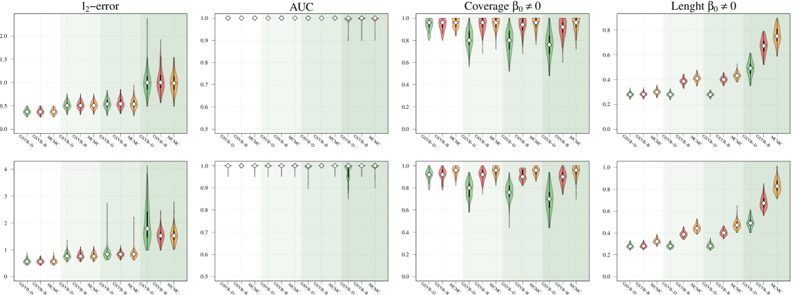
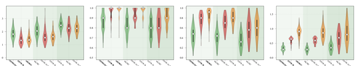
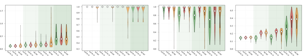
  Setting 1      Setting 2      Setting 3      Setting 4

  GSVB-D      GSVB-B      MCMC

Figure 1: Performance evaluation of GSVB and MCMC for Settings 1–4 with $p=1\!,000$ across 100 runs. For each method the white diamond ($\diamond$) indicates the median of the metric, the thick black line ( ) the interquartile range, and the black line ( ) 1.5 times the interquartile range. Rows 1–2: Gaussian family with $(n,m,s)=(200,5,5),(200,5,10)$. Row 3: Binomial family with $(n,m,s)=(400,5,5)$. Row 4: Poisson family with $(n,m,s)=(400,5,2)$. Note that for the Binomial family Setting 1 results in perfect separation of classes and is excluded from the study

Regarding coverage, whilst MCMC shows slightly better performance compared to GSVB, the proposed method still provides credible sets that capture a significant portion of the true non-zero coefficients (particularly GSVB-B). However, the credible sets of the variational posterior are sometimes not large enough to capture the true non-zero coefficients. This observation is further supported by the size of the marginal credible sets, with MCMC producing the largest sets, followed by GSVB-B and GSVB-D. These findings confirm the well-known fact that VB tends to underestimate the posterior variance (Carbonetto and Stephens, 2012; Blei et al., 2017; Zhang et al., 2019; Ray et al., 2020).

Interestingly, the set size is larger under $\mathcal{Q}^{\prime}$, highlighting the fact that the mean field variational family ($\mathcal{Q}$) lacks the necessary flexibility to accurately capture the underlying structure in the data. Furthermore, this result indicates that the full marginal credible quantity improves through the consideration of the interactions within the group.

5.3 Large scale simulations

In this section, our proposed approach is compared against SSGL (Bai et al., 2020) a state-of-the-art Bayesian method. Notably, SSGL employs a similar prior to that introduced in (2), however the multivariate Dirac mass on zero is replaced with a multivariate double exponential distribution, giving a continuous mixture with one density acting as the spike and the other as the slab, parameterized by $\lambda_{0}$ and $\lambda_{1}$ respectively. Under this prior Bai et al. (2020) derive an EM algorithm, which allows for fast updates, however, only MAP estimates are returned, meaning a posterior distribution for $\beta$ is not available. In addition, the performance of the proposed method is evaluated on larger datasets. As both methods are scalable with $p$, in this section it is increased to $p=5,000$. Both the sample size and the number of active (non-zero) groups, $s$ are varied as illustrated in Figure 2.

In this comparison, we set $\lambda_{1}=1$ for SSGL meaning the slab is identical between the two methods. For the spike for SSGL we took a value of $\lambda_{0}=100$ for the Gaussian and Poisson family and $\lambda_{0}=20$ under the Binomial family. These values were selected to ensure that sufficient mass is concentrated about zero without turning to cross validation to select the value. Finally, we let $a_{0}=1$ and $b_{0}=M$ for both methods.

Given that SSGL only returns a point estimate for the vector of coefficients $\beta$, the methods are compared in terms of $\ell_{2}$-error between the estimated coefficient and the true one, as well as in terms of AUC using the group inclusion probabilities. Overall GSVB performs comparatively or better than SSGL in most settings, obtaining a lower $\ell_{2}$-error and higher AUC (Figure 2). As expected, across the different methods there is a decrease in performance as the difficulty of the setting increases, meaning all methods perform better when there is less correlation in the design matrix. We note that the runtime of SSGL is marginally faster than our method in Settings 1-3, and faster in Settings 4. This is explained by the fact that SSGL only provides point estimate for $\beta$, rather than the full posterior distribution. A full breakdown of the runtimes is presented in Section D.2 of the Supplementary Material. Within this large scale simulation our method provides excellent uncertainty quantification. In particular, GSVB–B provides better coverage of the non-zero coefficients than GSVB–D, which can be justified by the set size. As in our comparison to MCMC we notice that there is an increase in the posterior set size as the difficulty of the setting increases, i.e. when there is an increase in the correlation of the design matrix.

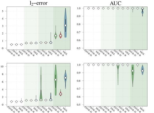
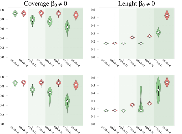
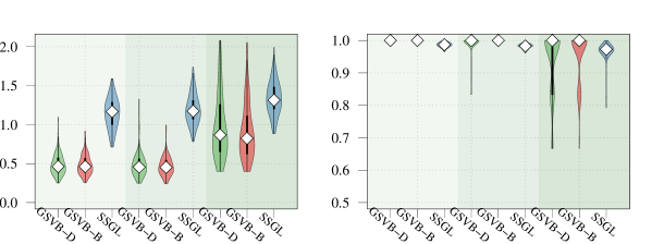
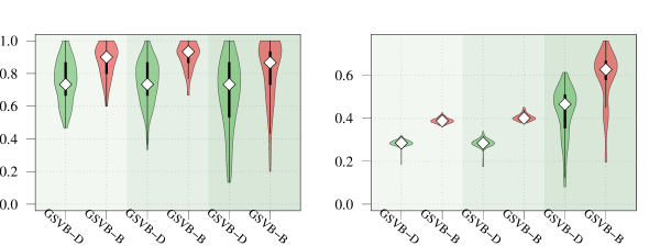
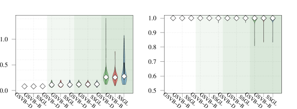
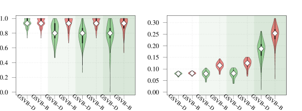
  Setting 1      Setting 2      Setting 3      Setting 4

  GSVB-D      GSVB-B      SSGL  

Figure 2: Performance evaluation of GSVB and SSGL for Settings 1–4 with $p=5\!,000$ across 100 runs. For each method the white diamond ($\diamond$) indicates the median of the metric, the thick black line ( ) the interquartile range, and the black line ( ) 1.5 times the interquartile range. Rows 1 – 2: Gaussian family with $(n,m,s)=(500,10,10),(500,10,20)$. Row 3: Binomial family with $(n,m,s)=(1000,5,5)$. Row 4: Poisson family with $(n,m,s)=(1000,5,3)$. Note that for the Binomial family Setting 1 results in perfect separation of classes and is excluded from the study.

6 Real data analysis

This section presents the analysis of two real world datasets with a third dataset analysis included in the Supplementary Material. The first problem is a linear regression problem wherein $p\gg n$ for which GSVB and SSGL are applied. The second is a logistic regression problem where $p<n$, for which the logistic group LASSO is applied in addition to GSVB and SSGL. As before, $a_{0}=1$, $b_{0}=M$ and GSVB was ran with a value of $\lambda=1$. For SSGL, we let $\lambda_{1}=1$ and $\lambda_{0}$ was chosen via five fold cross validation on the training set.

Overall, our results highlight that GSVB achieves state-of-the-art performance, producing parsimonious models with excellent predictive accuracy. Furthermore, in our analysis of the two datasets, variational posterior predictive distributions are constructed. These highlight the practical utility of GSVB, demonstrating how uncertainty in the predictions is quantified – an added benefit otherwise not available via MAP methods such as SSGL.

6.1 Bardet-Biedl Syndrome Gene Expression Study

The first dataset we examine is of microarray data, consisting of gene expression measurements for 120 laboratory rats. Originally the dataset was studied by Scheetz et al. (2006) and has subsequently been used to demonstrate the performance of several group selection algorithms (Huang and Zhang, 2010; Breheny and Huang, 2015; Bai et al., 2020). Briefly, the dataset consists of normalized microarray data harvested from the eye tissue of 12 week old male rats. The outcome of interest is the expression of TRIM32 a gene known to cause Bardet-Biedl syndrome, a genetic disease of multiple organs including the retina.

To pre-process the original dataset, which consists of $31,\!099$ probe sets (the predictors), we follow Breheny and Huang (2015) and select the $5,\!000$ probe sets which exhibit the largest variation in expression on the log scale. Further, following Breheny and Huang (2015) and Bai et al. (2020) a non-parametric additive model is used, wherein, $y_{i}=\mu+\sum_{j=1}^{p}f_{j}(x_{ij})+\epsilon_{i}$ with $\epsilon_{i}\sim N(0,\tau^{2})$ and $f_{j}:\mathbb{R}\rightarrow\mathbb{R}$. Here, $y_{i}\in\mathbb{R}$ corresponds to the expression of TRIM32 for the $i$th observation, and $x_{ij}$ the expression of the $j$th probe set for the $i$th observation. To approximate $f_{j}$ a three term natural cubic spline basis expansion is used. The resulting processing gave a group regression problem with $n=120$ and $M=1,\!000$ groups of size $m=3$. Denoting by $\phi_{j,k}$ the $k$th basis for $f_{j}$, we have

$$y_{i}=\mu+\sum_{j=1}^{M}\sum_{k=1}^{m}\phi_{j,k}(x_{ij})+\epsilon_{i}\;.$$ (24)

The performance of the methods is evaluated a ten-fold cross validation, where the methods are fit to the validation set and the test set is used for evaluation. More details about the computation of the metrics used to assess method performance can be found in the Supplementary Material.Overall, GSVB performed excellently, in particular GSVB–D obtained a smaller 10-fold cross validated MSE and model size than SSGL, meaning the models produced are parsimonious and comparably predictive to those of SSGL (Table 1). Furthermore, the PP coverage is excellent, particularly for GSVB–D which has a larger PP coverage than GSVB–B, whilst also having a smaller PP interval length.

Method MSE Num. selected groups PP. coverage PP. length GSVB-D 0.017 (0.019) 1.10 (0.316) 0.983 (0.035) 0.5460 (0.100) GSVB-B 0.018 (0.013) 1.50 (0.527) 0.950 (0.070) 0.5673 (0.091) SSGL 0.019 (0.001) 2.30 (1.060) – –

Table 1: Bardet-Biedl Syndrome Gene Expression Study, evaluation metrics computed on the held out test data. Average (sd.) over the 10 folds for the metrics are provided: mean squared error, number of selected groups, posterior predictive coverage, and mean posterior predictive interval length. Notably, GSVB failed to converge on the third fold.

To identify genes associated with TRIM32 expression, GSVB was ran on the full dataset. Both methods identify one gene each, with GSVB–D identifying Clec3a and GSVB–B identifying Slc25a34. Interestingly, the MSE was $0.012$ and $0.008$ for each method, suggesting Slc25a34 is more predictive of TRIM32 expression. Further, the PP coverage was $0.960$ for both methods and the PP interval length was $0.460$ and $0.367$ for GSVB–D and GSVB–B, reflecting there is less uncertainty in the prediction under GSVB–B.

6.2 MEMset splice site detection

The following application is based on the prediction of short read DNA motifs, a task which plays an important role in many areas of computational biology. For example, in gene finding, wherein algorithms such as GENIE (Burge and Karlin, 1997) rely on the prediction of splice sites (regions between coding and non-coding DNA segments).

The MEMset donor data has been used to build predictive models for splice sites and consists of a large training and test set. The original training set contains 8,415 true and 179,438 false donor sites and the test set 4,208 true and 89,717 false donor sites. The predictors are given by 7 factors with 4 levels each (A, T, C, G), a more detailed description is given in Yeo and Burge (2004). Initially analyzed by Yeo and Burge (2004), the data has subsequently been used by Meier et al. (2008) to evaluate the logistic group LASSO.

To create a predictive model we follow Meier et al. (2008) and consider all $3$rd order interactions of the 7 factors, which gives a total of $M=64$ groups and $p=1,156$ predictors. To balance the sets we randomly sub-sampled the training set without replacement, creating a training set of 1,500 true ($Y=1$) and 1,500 false donor sites. Regarding the test set a balanced set of 4,208 true and 4,208 false donor sites was created.

In addition to GSVB, we fit SSGL and group LASSO (used in the original analysis), for which we performed 5-fold cross validation to tune the hyperparameters. To assess the different methods, we use the test data, dividing it into 10 folds, and reporting the: (i) precision $\left(\frac{\text{TP}}{\text{TP + FP}}\right)$, (ii) recall $\left(\frac{\text{TP}}{\text{TP + FN}}\right)$, (iii) F-score $\left(\frac{\text{TP}}{\text{TP + 0.5FP + 0.5FN}}\right)$, (iv) AUC, and (v) the maximum correlation coefficient between true class membership and the predicted membership over a range of thresholds, $\rho_{\max}$, as used in Yeo and Burge (2004) and Meier et al. (2008). In addition we report (vi) the number selected groups, which for the group LASSO is given by the number which have a non-zero $\ell_{2,1}$ norm.

Method Precision Recall F-score AUC $\rho_{\max}$ Num. selected groups GSVB–D 0.915 (0.013) 0.951 (0.011) 0.933 (0.009) 0.975 (0.004) 0.870 (0.016) 10 GSVB–B 0.916 (0.011) 0.958 (0.013) 0.936 (0.008) 0.975 (0.004) 0.875 (0.016) 12 SSGL 0.921 (0.012) 0.950 (0.011) 0.935 (0.009) 0.977 (0.004) 0.879 (0.015) 48 Group LASSO 0.924 (0.013) 0.952 (0.010) 0.938 (0.010) 0.977 (0.004) 0.882 (0.016) 60

Table 2: Memset splice site detection, evaluation metrics computed on the held out test data. The test set was split into 10 folds and the mean (sd.) of the metrics are computed.

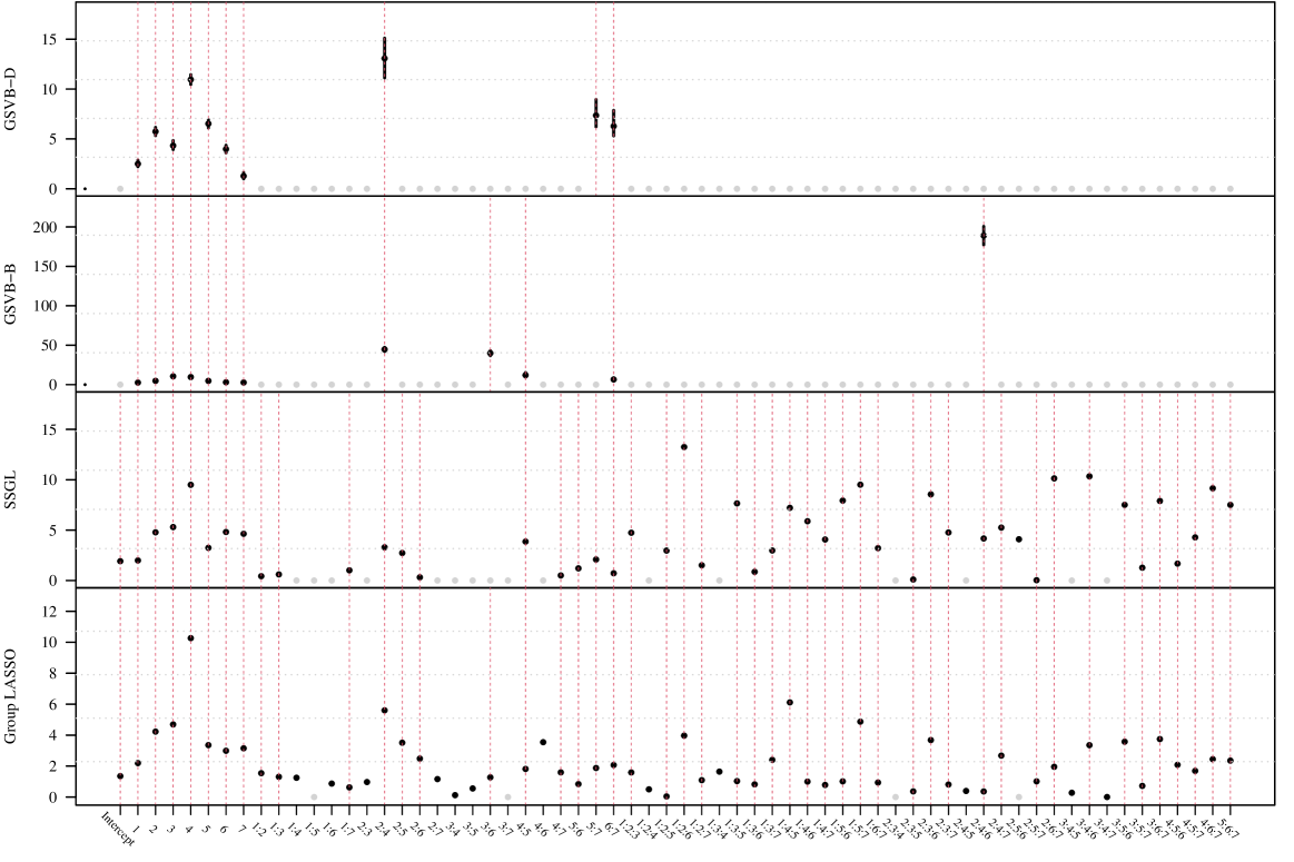
  Groups selected by more than one method     $\bullet$  Groups for which $\|\beta_{G_{k}}\|=0$

$\bullet$  Groups for which $\|\widehat{\beta}_{G_{k}}\|\neq 0$       95% credible intervals for $\|\beta_{G_{k}}\|$ where available   

Figure 5: MEMset splice site detection, comparison of $\ell_{2}$-norms for each group of coefficients $\widehat{\beta}_{G_{k}}$ for $k=1,\dots,64$. The red dotted line ( ​) shows groups which have been selected by more than one method. The points indicate $\|\widehat{\beta}_{G_{k}}\|$ where $\widehat{\beta}_{G_{k}}$ is the posterior mean for GSVB, the MAP for SSGL and the MLE estimate under the group LASSO. The points are coloured in black ($\bullet$) when they are non-zero and grey ( $\bullet$) otherwise. Finally when available the 95% credible set for $\|\beta_{G_{k}}\|$ is given by the solid black line ( ).

Overall the methods performed comparably. With GSVB–D obtaining the largest recall and the group LASSO the largest precision, F-score, AUC, and $\rho_{\max}$ by a small margin (Table 2). However, GSVB returned models that were of smaller size and therefore more parsimonious than those of SSGL and the group LASSO. This is further highlighted in Figure 5 (found in the Supplementary Material), which showcases the fact that the models obtained by GSVB are far simpler, selecting groups 1–7 as well as the interactions between groups 2:4 and 6:7 for both methods, with GSVB–D selecting 5:7 and GSVB–B selecting 2:6, 4:6 and 2:4:6 in addition to these. Further, Figure 5 showcases the fact that uncertainty is available about the norms of the groups.

7 Discussion

In this manuscript we have introduced GSVB, a scalable method for group sparse general linear regression. We have shown how a fast co-ordinate ascent variational inference algorithms can be constructed and used to compute the variational posterior. We have provided theoretical guarantees for the proposed VB approach in the setting of grouped spare linear regression by extending the theoretical work of Castillo et al. (2015) and Ray and Szabó (2022) for group sparse settings. Through extensive numerical studies we have demonstrated that GSVB provides state-of-the-art performance, offering a computationally inexpensive substitute to MCMC, whilst also performing comparably or better than MAP methods. Additionally, through our analysis of real world datasets we have highlighted the practical utility of our method. Demonstrating, that GSVB provides parsimonious models with excellent predictive performance, and as demonstrated in Section E.1, selects variables with established biological significance. Finally, different to MAP and frequentist methods, GSVB provides scalable uncertainty quantification, which serves as a powerful tool in several application areas.

SUPPLEMENTARY MATERIAL

Appendix A Co-ordinate ascent algorithms

Derivations are presented for the variational family $\mathcal{Q}^{\prime}$, noting that $\mathcal{Q}\subset\mathcal{Q}^{\prime}$, hence the update equations under $\mathcal{Q}$ follow directly from those under $\mathcal{Q}^{\prime}$. Recall, the family is given as,

$$\mathcal{Q}^{\prime}=\left\{Q^{\prime}(\mu,\Sigma,\gamma)=\bigotimes_{k=1}^{M}Q_{k}^{\prime}(\mu_{G_{k}},\Sigma_{G_{k}},\gamma_{k}):=\bigotimes_{k=1}^{M}\left[\gamma_{k}\ N\left(\mu_{G_{k}},\Sigma_{G_{k}}\right)+(1-\gamma_{k})\delta_{0}\right]\right\}$$ (25)

where $\Sigma\in\mathbb{R}^{p\times p}$ is a covariance matrix for which $\Sigma_{ij}=0$, for $i\in G_{k},j\in G_{l},k\neq l$ (i.e. there is independence between groups) and $\Sigma_{G_{k}}=(\Sigma_{ij})_{i,j\in G_{k}}\in\mathbb{R}^{m_{k}\times m_{k}}$ denotes the covariance matrix of the $k$th group.

A.1 Gaussian Family

Under the Gaussian family, $Y_{i}\overset{\text{iid}}{\sim}N(x_{i}^{\top}\beta,\tau^{2})$, and the $\log$-likelihood is given by,

$$\ell(\mathcal{D};\beta,\tau^{2})=-\frac{n}{2}\log(2\pi\tau^{2})-\frac{1}{2\tau^{2}}\|y-X\beta\|^{2}.$$

Recall, we have chosen to model $\tau^{2}$ by an inverse-Gamma prior which has density,

$$\frac{b^{a}}{\Gamma(a)}x^{-a-1}\exp\left(\frac{-b}{x}\right)$$

where $a,b>0$ and in turn we extend $\mathcal{Q}^{\prime}$ to $\mathcal{Q}^{\prime}_{\tau}=\mathcal{Q}^{\prime}\times\{\Gamma^{-1}(a^{\prime},b^{\prime}):a^{\prime},b>0\}$.

Under this variational family, the expectation of the negative log-likelihood is given by,

$$\mathbb{E}_{Q^{\prime}_{\tau}} \left[-\ell(\mathcal{D};\beta)\right]=\mathbb{E}_{Q^{\prime}_{\tau}}\left[\frac{n}{2}\log(2\pi\tau^{2})+\frac{1}{2\tau^{2}}\|y-X\beta\|^{2}\right]$$

$$= \ \mathbb{E}_{Q^{\prime}_{\tau}}\left[\frac{n}{2}\log(2\pi\tau^{2})+\frac{1}{2\tau^{2}}\left(\|y\|^{2}+\|X\beta\|^{2}-2\langle y,X\beta\rangle\right)\right]$$

$$= \ \frac{n}{2}(\log(2\pi)+\log(b^{\prime})-\kappa(a^{\prime}))$$

$$+ \ \frac{a^{\prime}}{2b^{\prime}}\Bigg{(}\|y\|^{2}+\left(\sum_{i=1}^{p}\sum_{j=1}^{p}(X^{\top}X)_{ij}\mathbb{E}_{Q^{\prime}_{\tau}}\left[\beta_{i}\beta_{j}\right]\right)-2\sum_{k=1}^{M}\gamma_{k}\langle y,X_{G_{k}}\mu_{G_{k}}\rangle\Bigg{)}$$ (26)

where the expectation

$$\mathbb{E}_{Q^{\prime}_{\tau}}\left[\beta_{i}\beta_{j}\right]=\begin{cases}\gamma_{k}\left(\Sigma_{ij}+\mu_{i}\mu_{j}\right)&\quad i,j\in G_{k}\\ \gamma_{k}\gamma_{h}\mu_{i}\mu_{j}&\quad i\in G_{k},j\in G_{h},h\neq k\end{cases}$$

A.2 Binomial Family Re-parameterization

To re-parametrization of $\Sigma_{G_{k}}$ we follow the same process as in Section 3.2.1. Formally, we have,

$$\Sigma_{G_{k}}=(X^{\top}_{G_{k}}A_{t}X_{G_{k}}+wI)^{-1}$$ (27)

where $w\in\mathbb{R}$ is the free parameter to be optimized and $A_{t}=\operatorname{diag}(a(t_{1}),\dots,a(t_{n}))$. Notably, this result follows due to the quadratic nature of the bound employed. Meaning we are able to re-parameterize $\Sigma_{G_{k}}$.

Appendix B Derivation of Variational Posterior Predictive

To compute the variational posterior predictive distribution for the Binomial and Poisson model, we sample $\beta\sim\tilde{\Pi}$ and then sample $y^{*}|x^{*},\mathcal{D}$ from the respective distribution with mean given by $f(x*^{\top}\beta)$ where $x^{*}\in\mathbb{R}^{p}$ and $f$ is the link function. To sample from $\tilde{\Pi}$ we sample $z_{k}\overset{\text{ind}}{\sim}\text{Bernoulli}(\gamma_{k})$ and then $\beta_{G_{k}}\overset{\text{ind}}{\sim}N(\mu_{G_{k}},\Sigma_{G_{k}})$ if $z_{k}=1$ otherwise we set $\beta_{G_{k}}=0_{m_{k}}$.

For the Gaussian family we are able to simplify the process by integrating out the variance $\tau^{2}$. Following Murphy (2007), substituting $\xi=\tau^{2}$ and recalling the independence of $\tau^{2}$ and $\beta$ in our variational family, we have,

$$\tilde{p}(y^{\ast}|x^{\ast},\mathcal{D}) \ \propto\int_{\mathbb{R}^{p}}\int_{R^{+}}\xi^{-(a^{\prime}+1/2)-1}\exp\left(-\frac{(y^{\ast}-x^{\ast\top}\beta)^{2}+2b^{\prime}}{2\xi}\right)\ d\xi\ d\tilde{\Pi}(\beta)$$

$$\ \propto\int_{\mathbb{R}^{p}}\left(\frac{(y^{\ast}-x^{\ast\top}\beta)^{2}}{2b^{\prime}}+1\right)^{-(a^{\prime}+1/2)}\ d\tilde{\Pi}(\beta)$$

Recognizing that the expression within the integral has the same functional form as a generalized $t$-distribution, whose density is denoted as $t(x;\mu,\sigma^{2},\nu)=\Gamma((\nu+1)/2)/(\Gamma(\nu/2)\sqrt{\nu\pi}\sigma)(1+(x-\mu)^{2}/(\nu\sigma^{2}))^{-(\nu+1)/2}$, yields,

$$\tilde{p}(y^{\ast}|x^{\ast},\mathcal{D})=\int_{\mathbb{R}^{p}}t(y^{\ast};x^{\ast\top}\beta,b^{\prime}/a^{\prime},2a^{\prime})\ d\tilde{\Pi}(\beta)$$ (28)

As (28) is intractable we instead sample from $p(y^{\ast}|x^{\ast},\mathcal{D})$, by

1. Sampling $\beta\sim\tilde{\Pi}$.

2. Sampling $y^{\ast}$ from $Y^{\ast}=\mu+\sigma t_{\nu}$ where $\mu=x^{\ast\top}\beta,\sigma=\sqrt{b^{\prime}/a^{\prime}}$ and $\nu=2a^{\prime}$, where $t_{\nu}$ denotes a t-distribution with $\nu$ degrees of freedom.

Appendix C Gibbs Sampler

We present a Gibbs sampler for the Gaussian family of models, noting that the samplers for the Binomial and Poisson family use the same principles. We begin by considering a slight alteration of the prior given in (2). Formally,

$$\beta_{G_{k}}\overset{\text{ind}}{\sim} \ \Psi(\beta_{G_{k}};\lambda)$$ (29)

$$z_{k}|\theta_{k}\overset{\text{ind}}{\sim} \ \text{Bernoulli}(\theta_{k})$$

$$\theta_{k}\overset{\text{iid}}{\sim} \ \text{Beta}(a_{0},b_{0})$$

for $k=1,\dots,M$ and $\tau^{2}=\xi\overset{\text{iid}}{\sim}\Gamma^{-1}(\xi;a,b)$. Under this prior writing the likelihood as,

$$p(\mathcal{D}|\beta,z,\xi)=\prod_{i=1}^{n}\phi\left(y_{i};f\left(\sum_{k=1}^{M}z_{k}\langle x_{G_{k}},\beta_{G_{k}}\rangle\right),\xi\right)$$ (30)

where $\phi(\cdot;\mu,\sigma^{2})$ is the density of the Normal distribution with mean $\mu$ and variance $\sigma^{2}$, and $f$ is the link function (which in this case is the identity), yields the posterior

$$p(\beta,z,\xi|\mathcal{D})\propto p(\mathcal{D}|\beta,z,\xi)\pi(\xi)\prod_{k=1}^{M}\pi(\beta_{G_{k}})\pi(z_{k}|\theta_{k})\pi(\theta_{k}).$$ (31)

Notably, the posterior is equivalent to our previous formulation.

To sample from (31), we construct a Gibbs sampler as outlined in Algorithm 2. Ignoring the superscript for clarity, the distribution $\theta_{k}|\mathcal{D},\beta,z,\theta_{-k},\xi$ is conditionally independent of $\mathcal{D},\beta,z_{-k},\xi$ and $\theta_{-k}$. Therefore, $\theta_{k}$ is sampled from $\theta_{k}|z_{k}$, which has a $\text{Beta}(a_{0}+z_{k},b_{0}+1-z_{k})$ distribution. Regarding $z_{j}^{(i)}$, the conditional density

$$p(z_{k}|\mathcal{D},\beta,z_{-k},\theta,\xi)\propto \ p(\mathcal{D}|\beta,z_{-k},z_{k},\theta,\xi)\pi(z_{k}|\beta,z_{-k},\theta,\xi).$$

$$= \ p(\mathcal{D};\beta,z,\xi)\pi(z_{k}|\theta_{k}).$$ (32)

As $z_{k}$ is discrete, evaluating the RHS of (C) for $z_{k}=0$ and $z_{k}=1$, gives the unnormalised conditional probabilities. Summing gives the normalisation constant and thus we can sample $z_{k}$ from a Bernoulli distribution with parameter

$$p_{k}=\frac{p(z_{k}=1|\mathcal{D},\beta,z_{-k},\theta,\xi)}{p(z_{k}=0|\mathcal{D},\beta,z_{-k},\theta,\xi)+p(z_{k}=1|\mathcal{D},\beta,z_{-k},\theta,\xi)}.$$ (33)

Finally, regarding $\beta_{G_{k},j}^{(i)}$ we use a Metropolis-Hastings within Gibbs step, wherein a proposal $\beta_{G_{k},j}^{(i)}$ is sampled from a random-walk proposition kernel $K$, where in our implementation $K(x|\vartheta,\varepsilon)=N(x;\vartheta,\sqrt{2}\left(10^{1-\varepsilon}\right)^{1/2})$. The proposal is then accepted with probability $A$ or rejected with probability $1-A$, in which case $\beta_{G_{k},j}^{(i)}\leftarrow\beta_{G_{k},j}^{(i-1)}$, where $A$ is given by,

$$A=\min\left(1,\frac{p(\mathcal{D};\beta_{G_{k}^{c}},\beta_{G_{k},-j},\beta_{G_{k},j}^{(i)},z,\xi)\pi(\beta_{G_{k},j}^{(i)}|\beta_{G_{k},-j})}{p(\mathcal{D};\beta_{G_{k}^{c}},\beta_{G_{k},-j},\beta_{G_{k},j}^{(i-1)},z,\xi)\pi(\beta_{G_{k},j}^{(i-1)}|\beta_{G_{k},-j})}\frac{K(\beta_{j}^{(i-1)}|\beta_{j}^{(i)},z_{k}^{(i)})}{K(\beta_{j}^{(i)}|\beta_{j}^{(i-1)},z_{k}^{(i-1)})}\right)$$

Algorithm 2 MCMC sampler for the Gaussian family GSpSL regression

Initialize $\beta^{(0)},z^{(0)},\theta^{(0)},\xi^{(0)}$

for $i=1,\dots,N$ 

     for $k=1,\dots,M$ 

         $\theta^{(i)}_{k}\overset{\text{iid.}}{\sim}\text{Beta}(a_{0}+z_{k}^{(i-1)},b_{0}+1-z_{k}^{(i-1)})$      

     for $k=1,\dots,M$ 

         $z^{(i)}_{k}\overset{\text{ind.}}{\sim}\text{Bernoulli}(p_{k})$      

     for $k=1,\dots,M$ 

         for $j=1,\dots,m_{k}$ 

              $\beta_{G_{k},j}^{(i)}\sim p(\beta_{G_{k},j}^{(i)}|\mathcal{D},z^{(i)},\beta^{(i)}_{G_{1:k-1}},\beta_{G_{k,1:j-1}}^{(i)},\beta_{G_{k,j+1:m_{k}}}^{(i-1)},\beta_{G_{k+1:M}}^{(i-1)},\xi^{(i-1)})$               

     Sample $\xi^{(i)}\overset{\text{iid.}}{\sim}\Gamma^{-1}(a+0.5n,b+0.5\|y-\sum_{k=1}^{M}z_{k}X_{G_{k}}\beta_{G_{k}}^{(i)}\|^{2})$

return $\{\beta^{(i)},z^{(i)},\theta^{(i)},\xi^{(i)}\}_{i=1}^{N}$.

Appendix D Numerical Study

D.1 Performance with large groups

The performance of GSVB with large groups is examined. For this we fix $(n,p,s)=(1\!,000,5\!,000,10)$ and vary the group size to be $m=10,20,25,50,100$. The results, presented in Figure 3 highlight that the performance of the method is excellent for groups of size $m=10,20,25$, and begins to suffer when groups are of size $m=50$ and $100$, particularly in settings 3 and 4 wherein GSVB–B did not run.

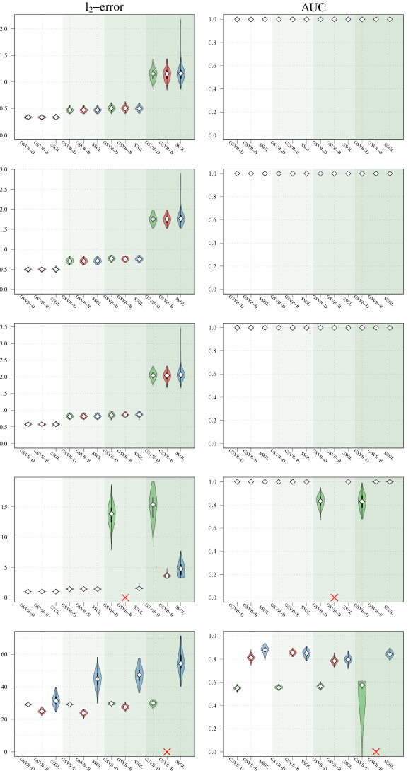
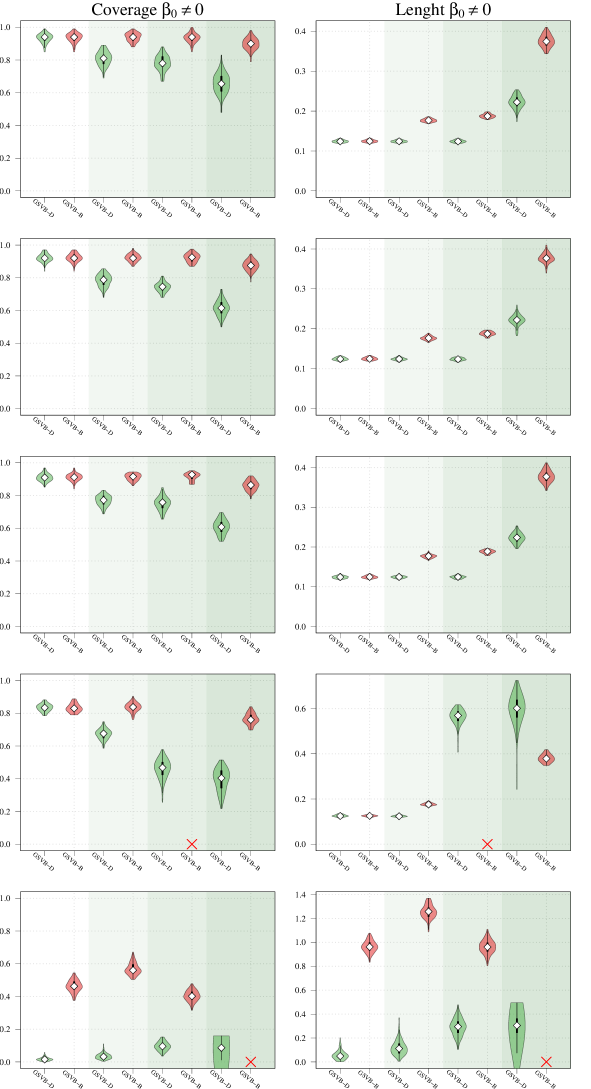
  Setting 1      Setting 2      Setting 3      Setting 4

$\times$ 95+ runs did not converge      GSVB-D      GSVB-B      SSGL

Figure 3: Performance evaluation of GSVB and SSGL for Settings 1–4 with $(n,p,s)=(1\!,000,5\!,000,10)$ across 100 runs. For each method the white diamond ($\diamond$) indicates the median of the metric, the thick black line ( ) the interquartile range, and the black line ( ) 1.5 times the interquartile range. Rows 1–5: Gaussian family with increasing group sizes of $m=10,20,25,50,100$.

D.2 Runtime

Runtimes for the experiments presented in Section 5 are presented in Table 3 and Table 4. Notably, the runtime for GSVB over MCMC is orders of magnitudes faster. The runtime of GSVB in comparison to SSGL is slower in Settings 4, but marginally slower in the remaining settings. Note all simulations were ran on AMD EPYC 7742 CPUs (128 core, 1TB RAM).

Method Setting 1 Setting 2 Setting 3 Setting 4 Gaus. s=5 GSVB–D 2.1s (1.6s, 3.0s) 1.8s (1.1s, 2.9s) 3.5s (1.6s, 8.0s) 2.2s (1.6s, 5.2s) GSVB–B 1.8s (1.2s, 2.9s) 2.0s (1.3s, 3.1s) 3.4s (1.7s, 7.3s) 2.6s (1.8s, 6.7s) MCMC 7m 53s (7m 31s, 8m 12s) 7m 55s (7m 34s, 8m 2s) 7m 44s (7m 20s, 7m 48s) 8m 14s (7m 49s, 8m 17s) Gaus. s=10 GSVB–D 2.3s (1.7s, 3.8s) 2.6s (1.9s, 3.9s) 7.4s (2.9s, 9.7s) 4.2s (2.4s, 12.1s) GSVB–B 2.9s (1.8s, 4.5s) 2.6s (2.2s, 3.2s) 9.5s (4.8s, 13.9s) 4.3s (2.7s, 14.0s) MCMC 9m 55s (9m 45s, 10m 8s) 10m 13s (9m 48s, 10m 30s) 9m 19s (9m 24s, 9m 33s) 10m 11s (9m 46s, 10m 27s) Binom. s=3 GSVB–D - 5.5s (3.5s, 9.3s) 7.7s (3.7s, 12.0s) 5.2s (2.7s, 8.0s) GSVB–B - 7.2s (6.0s, 11.9s) 7.8s (5.6s, 14.4s) 6.0s (3.7s, 9.5s) MCMC - 16m 45s (16m, 17m 15s) 16m 45s (15m 45s, 17m) 15m 45s (14m 49s, 16m 30s) Pois. s=2 GSVB–D 3.6s (3.3s, 4.1s) 3.3s (2.9s, 3.7s) 3.1s (2.9s, 5.2s) 3.4s (2.4s, 4.1s) GSVB–B 12.5s (10.0s, 18.0s) 10.1s (7.9s, 14.5s) 15.5s (10.1s, 41.6s) 13.3s (10.5s, 24.0s) MCMC 15m 45s (14m 49s, 16m 45s) 15m 45s (15m 15s, 16m 30s) 16m (14m 59s, 18m) 18m 30s (16m 45s, 19m 45s)

Table 3: Median (5%, 95% quartile) runtimes for numerical experiments presented in Figure 1. Note $(n,p)=(200,1000)$ for the Gaussian family and $(n,p)=(400,1000)$ for the Binomial and Poisson family. Note that under setting 1 for the Binomial family there is perfect separation.

Method Setting 1 Setting 2 Setting 3 Setting 4 Gaus. m=10, s=10 GSVB–D 59.1s (47.2s, 1m 16s) 54.3s (47.5s, 1m 8s) 2m 53s (1m 4s, 6m 35s) 8m 7s (4m 30s, 25m 36s) GSVB–B 57.7s (50.7s, 1m 18s) 57.0s (49.5s, 1m 14s) 2m 51s (1m 7s, 6m 38s) 9m 45s (4m 53s, 25m 40s) SSGL 1m 3s (59.5s, 1m 13s) 50.8s (41.6s, 59.5s) 1m 1s (58.1s, 1m 16s) 1m 24s (1m 11s, 2m 3s) Gaus. m=10, s=20 GSVB–D 3m 7s (3m 46s, 4m 31s) 3m 13s (3m 42s, 4m 39s) 9m 42s (3m 56s, 14m 54s) 20m 48s (6m 38s, 39m 23s) GSVB–B 3m 29s (3m 6s, 4m 20s) 3m 23s (3m 57s, 4m 48s) 12m 18s (4m 59s, 16m 20s) 34m 59s (12m 54s, 45m 2s) SSGL 2m 42s (1m 23s, 2m 3s) 1m 16s (59.2s, 2m 40s) 2m 6s (2m 37s, 2m 30s) 2m 16s (2m 31s, 6m 32s) Binom. m=5, s=5 GSVB–D - 3m 43s (2m 54s, 4m 54s) 2m 26s (2m 34s, 4m 5s) 2m 50s (1m 16s, 3m 30s) GSVB–B - 4m 32s (3m 40s, 5m 8s) 3m 26s (2m 20s, 5m 26s) 2m 25s (2m 47s, 5m 18s) SSGL - 2m 54s (2m 44s, 3m 42s) 3m 33s (2m 57s, 3m 26s) 2m 40s (2m 31s, 2m 3s) Pois. m=5, s=3 GSVB–D 16.3s (9.8s, 21.5s) 11.2s (8.2s, 20.8s) 16.0s (10.4s, 43.0s) 12.9s (8.6s, 48.7s) GSVB–B 2m 26s (2m 59s, 3m 20s) 2m 55s (1m 29s, 3m 20s) 3m 53s (2m 49s, 9m 25s) 3m 33s (2m 4s, 9m 11s) SSGL 4m 11s (3m 49s, 8m 38s) 4m 34s (2m 11s, 13m 4s) 2m 29s (2m 56s, 16m 33s) 2m 32s (1m 25s, 3m 2s)

Table 4: Median (5%, 95% quartile) runtimes for numerical experiments presented in Figure 2. Note $(n,p)=(500,5000)$ for the Gaussian family and $(n,p)=(1000,5000)$ for the Binomial and Poisson family. Note that under setting 1 for the Binomial family there is perfect separation

Appendix E Real data analysis

E.1 Genetic determinants of Low-density Lipoprotein in mice

Here we analyze a dataset from the Mouse Genome Database (Blake et al., 2021) and consists of $p=10,\!346$ single nucleotide polymorphisms (SNPs) collected from $n=1,\!637$ laboratory mice. Notably, each SNP, $x_{ij}$ for $j=1,\dots,p$ and $i=1,\dots,n$, takes a value of 0, 1 or 2. This value indicates how many copies of the risk allele are present. Alongside the genotype data, a phenotype (response) is also collected. The phenotype we consider is low-density lipoprotein cholesterol (LDL-C), which has been shown to be a major risk factor for conditions like coronary artery disease, heart attacks, and strokes (Silverman et al., 2016).

To pre-process the original dataset SNPs with a rare allele frequency, given by $\text{RAF}_{j}=\frac{1}{2n}\sum_{i=1}^{n}\left(\mathbb{I}(x_{ij}=1)+2\mathbb{I}(x_{ij}=2)\right)$ for $j=1,\dots,p$, below the first quartile were discarded. Further, due to the high colinearity, covariates with $|\operatorname{corr}(x_{j},x_{k})|\geq 0.97$ for $k>j$, $j=1,\dots,p-1$, were removed. After pre-processing, $3,\!341$ SNPs remained. These were used to construct groups by coding each $x_{ij}:\{0,1,2\}\mapsto\{(0,0),(0,1),(1,1)\}$, in turn giving groups of size $m=2$.

To evaluate the methods ten fold cross validation is used. Specifically, methods are fit to the validation set and the test set is used for evaluation. This is done by computing the: (i) MSE between the true and predicted value of the response, given by $\frac{1}{\tilde{n}}\|y-X\widehat{\beta}\|$ where $\tilde{n}$ is the size of the test set, (ii) posterior predictive (PP) coverage, which measures the proportion of times the response is included in the 95% PP set, and (iii) the average size of the 95% PP set. In addition, (iv) the number of groups selected, given by $\sum_{k=1}^{M}\mathbb{I}(\gamma_{k}>0.5)$ is also reported.

Importantly the PP distribution is available for GSVB, and given by, $\tilde{p}(y^{\ast}|x^{\ast},\mathcal{D})=\int_{\mathbb{R}^{p}\times\mathbb{R}^{+}}p(y^{\ast}|\beta,\tau^{2},x^{\ast},\mathcal{D})\ d\tilde{\Pi}(\beta,\tau^{2})$ where $x^{\ast}\in\mathbb{R}^{p}$ is a feature vector (see Section B of the Supplementary material for details). In genetics studies, $x^{\ast\top}\beta$, is referred to as the polygenic risk score and is commonly used to evaluate genetic risk. While frequentist or MAP methods offer only point estimates, Figure 4 demonstrates that GSVB can offer a distribution for this score, highlighting the uncertainty associated with the estimate.

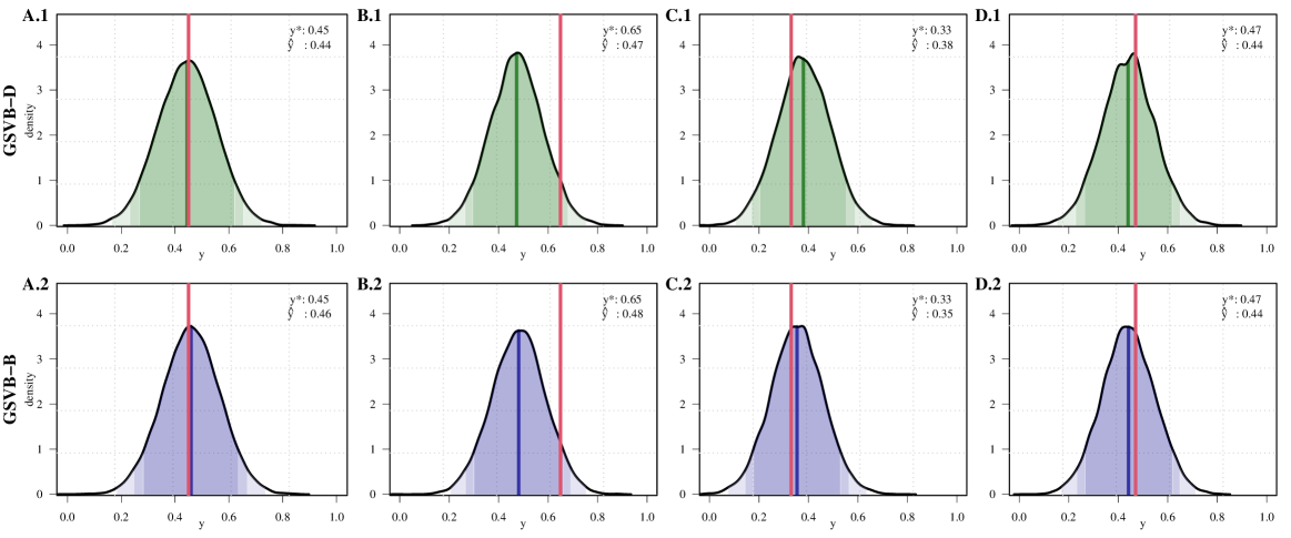
GSVB-D:    PP mean:     Mass%:     90%     95%     99%     Observed response GSVB-B:    PP mean:     Mass%:     90%     95%     99%

Figure 4: Genetic determinants of LDL-C in mice, variational posterior predictive distribution for GSVB-D (panels A.1 - D.1) and GSVB-B (panels A.2 - D.2) constructed for four observations in the held out test set (fold 1). Notably the red line ( ) represents the measured LDL-C level, with the adjacent text giving this value ($y^{*}$) and the posterior mean ($\widehat{y}$). The shading of the variational posterior indicates where $90\%$, $95\%$ and $99\%$ of the mass is contained.

Regarding the performance of each method results are presented in Table 5, these highlight that GSVB performs excellently obtaining parsimonious models with a comparable MSE to SSGL. In addition, GSVB provides impressive uncertainty quantification, yielding a coverage of $0.945$ and $0.941$ for GSVB–D and GSVB–B respectively. The SNPs selected by GSVB–D and GSVB-B are similar and reported in Table 6 of the Supplementary material. When the methods are fit to the full dataset, the SNPs selected by both method are: rs13476241, rs13477968, and rs13483814, with GSVB–B selecting rs13477939 in addition. Notably, rs13477968 corresponds to the Ago3 gene, which has been shown to play a role in activating LDL receptors, which in turn regulate LDL-C (Matsui et al., 2010).

Method	MSE	Num. selected groups	PP. coverage	PP. length
GSVB-D	0.012 (0.002)	3.50 (0.527)	0.945 (0.027)	0.425 (0.005)
GSVB-B	0.012 (0.002)	4.00 (0.667)	0.941 (0.029)	0.421 (0.005)
SSGL	0.012 (0.002)	57.40 (5.481)	-	-

Table 5: Genetic determinants of LDL-C in mice, evaluation of methods on the held out genotype data. Reported is the 10 fold cross validated MSE, the number of selected groups, the posterior predictive coverage, and mean posterior predictive interval length.

RSID (or probe ID)	Freq. GSVB-D	Freq. GSVB-B
rs13476279	6	6
rs13483823	6	5
CEL.4_130248229	5	3
rs13477968	3	5
rs13476241	4	3
CEL.X_65891570	2	4
rs13477903	2	2
rs3688710	2	1
rs13477939	1	-
rs3157124	1	-
rs13478204	-	3
rs6186902	-	2
rs13483814	-	1
rs4222922	-	1
rs6187266	-	1
UT_4_128.521481	-	1

Table 6: Genetic determinants of LDL-C in mice: SNPs selected by GSVB.

E.2 Bardet-Biedl Syndrome Gene Expression Study

Probe ID	Gene Name	Freq. GSVB-D	Freq. GSVB-B	Freq. SSGL
1383183_at		1	1	8
1386237_at		1	1	-
1397359_at		4	2	-
1386552_at		-	1	-
1378682_at		-	1	-
1385926_at		-	-	2
1396814_at		-	-	3
1386811_at	Hacd4	1	2	-
1386069_at	Sp2	4	2	-
1371209_at	RT1-CE5	-	1	-
1391624_at	Sec14l3	-	1	-
1383829_at	Bbx	-	2	-
1389274_at	Dcakd	-	-	1
1373995_at	Abcg1	-	-	1
1375361_at	Snx18	-	-	1
1368915_at	Kmo	-	-	7

Table 7: Bardet-Biedl syndrome gene expression study: variables selected by GSVB and SSGL.

E.3 MEMset splice site detection

Appendix F Proofs of asymptotic results

F.1 A general class of model selection priors and an overview of the proof

Our theoretical results apply to a wider class of model selection priors than the group spike and slab prior (2) underlying our variational approximation. In this section, we thus consider this more general class of model selection priors Castillo et al. (2015); Ning et al. (2020); Ray and Szabó (2022) defined hierarchically via:

$$\begin{split}s\sim\pi_{M}(s)&\\ S||S|=s\sim\text{Unif}_{M,s}&\\ \beta_{G_{k}}\sim^{ind}\begin{cases}\Psi_{\lambda,m_{k}}(\beta_{G_{k}}),~{}~{}&G_{k}\in S,\\ \delta_{0},&G_{k}\not\in S,\end{cases}\end{split}$$ (34)

where $\pi_{M}$ is a prior on $\{0,1,\dots,M\}$, $\text{Unif}_{M,s}$ is the uniform distribution on subsets $S\subseteq\{1,\dots,M\}$ of size $s$ and

$$\Psi_{\lambda,m_{k}}(\beta_{G_{k}})=\Delta_{m_{k}}\lambda^{m_{k}}\exp\left(-\lambda\|\beta_{G_{k}}\|_{2}\right)$$ (35)

is a density on $\mathbb{R}^{m_{k}}$ with $\Delta_{m_{k}}=2^{-m_{k}}\pi^{(1-m_{k})/2}\Gamma((m_{k}+1)/2)^{-1}$. This can be concisely written as

$$(S,\beta)\mapsto\pi_{M}(|S|)\frac{1}{{M\choose|S|}}\delta_{0}(S^{c})\prod_{G_{k}\in S}\Psi_{\lambda,m_{k}}(\beta_{G_{k}}).$$ (36)

Following Castillo et al. (2015); Ning et al. (2020); Ray and Szabó (2022), we assume as usual that

$$A_{1}M^{-A_{3}}\pi_{M}(s-1)\leq\pi_{M}(s)\leq A_{2}M^{-A_{4}}\pi_{M}(s-1),\qquad s=1,\dots,M.$$ (37)

We further recall the assumption (38) made on the scale parameter:

$$\underline{\lambda}\leq\lambda\leq 2\bar{\lambda},\qquad\qquad\underline{\lambda}=\frac{\|X\|}{M^{1/m_{\text{max}}}},\qquad\qquad\bar{\lambda}=3\|X\|\sqrt{\log M}.$$ (38)

The group spike and slab prior fits within this framework by taking $\pi_{M}=\text{Bin}(M,\tfrac{a_{0}}{a_{0}+b_{0}})$, and hence the following results immediately imply Theorems 1 and 2. Recall the parameter set

$$\mathcal{B}_{\rho_{n},s_{n}}=\{\beta_{0}\in\mathbb{R}^{p}:\phi(S_{\beta_{0}})\geq c_{0},~{}|S_{\beta_{0}}|\leq s_{n},~{}\widetilde{\phi}(\rho_{n}|S_{\beta_{0}}|)\geq c_{0}\}$$

defined in (23).

Theorem 3 (Contraction).

Suppose that Assumption (K) holds, the prior satisfies (37)-(38) and $s_{n}$ satisfies $m_{\text{max}}\log s_{n}\leq K^{\prime}\log M$ for some $K^{\prime}>0$. Then the variational posterior $\tilde{\Pi}$ based on either the variational family $\mathcal{Q}$ in (5) or $\mathcal{Q}^{\prime}$ in (6) satisfies, with $s_{0}=|S_{\beta_{0}}|$,

$$\sup_{\beta_{0}\in\mathcal{B}_{\rho_{n},s_{n}}}E_{\beta_{0}}\tilde{\Pi}\left(\beta:\|X(\beta-\beta_{0})\|_{2}\geq\frac{H_{0}\rho_{n}^{1/2}\sqrt{s_{0}\log M}}{\bar{\phi}(\rho_{n}s_{0})}\right)\to 0$$

$$\sup_{\beta_{0}\in\mathcal{B}_{\rho_{n},s_{n}}}E_{\beta_{0}}\widetilde{\Pi}\left(\beta:\|\beta-\beta_{0}\|_{2,1}\geq\frac{H_{0}\rho_{n}s_{0}\sqrt{\log M}}{\|X\|\bar{\phi}(\rho_{n}s_{0})^{2}}\right)\to 0,$$

$$\sup_{\beta_{0}\in\mathcal{B}_{\rho_{n},s_{n}}}E_{\beta_{0}}\widetilde{\Pi}\left(\beta:\|\beta-\beta_{0}\|_{2}\geq\frac{H_{0}\rho_{n}^{1/2}\sqrt{s_{0}\log M}}{\|X\|\widetilde{\phi}(\rho_{n}s_{0})^{2}}\right)\to 0,$$

for any $\rho_{n}\to\infty$ (arbitrarily slowly), $\mathcal{B}_{\rho_{n},s_{n}}$ defined in (23) and where $H_{0}$ depends only on the prior.

Theorem 4 (Dimension).

Suppose that Assumption (K) holds, the prior satisfies (37)-(38) and $s_{n}$ satisfies $m_{\text{max}}\log s_{n}\leq K^{\prime}\log M$ for some $K^{\prime}>0$. Then the variational posterior $\tilde{\Pi}$ based on either the variational family $\mathcal{Q}$ in (5) or $\mathcal{Q}^{\prime}$ in (6) satisfies

$$\sup_{\beta_{0}\in\mathcal{B}_{\rho_{n},s_{n}}}E_{\beta_{0}}\tilde{\Pi}\left(\beta:|S_{\beta}|\geq\rho_{n}|S_{\beta_{0}}|\right)\to 0$$

for any $\rho_{n}\to\infty$ (arbitrarily slowly) and $\mathcal{B}_{\rho_{n},s_{n}}$ defined in (23).

To prove Theorems 3 and 4, we use the following result which relates the VB probability of sets having exponentially small probability under the true posterior.

Lemma 1 (Theorem 5 of Ray and Szabó (2022)).

Let ${B}_{n}$ be a subset of the parameter space, $A_{n}$ be events and $Q_{n}$ be distributions for $\beta$. If there exists $C>0$ and $\delta_{n}>0$ such that

$$E_{\beta_{0}}\Pi(\beta\in{B}_{n}^{c}|Y)1_{A_{n}}\leq Ce^{-\delta_{n}},$$

then

$$E_{\beta_{0}}Q_{n}(\beta\in{B}_{n}^{c})1_{A_{n}}\leq\frac{2}{\delta_{n}}\left[E_{\beta_{0}}D_{\text{KL}}(Q_{n}\|\Pi(\cdot|Y))1_{A_{n}}+Ce^{-\delta/2}\right].$$

The proof thus reduces to finding events $A_{n}$ with $P_{\beta_{0}}(A_{n})\to 1$ on which:

1. The true posterior places only exponentially small probability outside $B_{n}$, that is $\Pi(B_{n}^{c}|Y)\leq Ce^{-\delta_{n}}$ for some rate $\delta_{n}\to\infty$,

2. The $D_{\text{KL}}$-divergence between the VB posterior $\tilde{\Pi}$ and the full posterior is $o(\delta_{n})$.

In our setting, we shall take $\delta_{n}=Cs_{0}\log M$. Full posterior results are dealt with in Section F.2, the $D_{\text{KL}}$-divergence in Section F.3 and the proofs of Theorems 3 and 4 are completed in Section F.4.

F.2 Asymptotic theory for the full posterior

We now establish contraction rates for the full computationally expensive posterior distribution, keeping track of the exponential tail bounds needed to apply Lemma 1. While the proofs in this section largely follow those in Castillo et al. Castillo et al. (2015), the precise arguments adapting these results to the group sparse setting are rather technical and hence we provide them for convenience. We first establish a Gaussian tail bound in terms of the group structure.

Lemma 2.

The event

$$\mathcal{T}_{0}=\left\{\max_{k=1,\dots,M}\|X_{G_{k}}^{T}(Y-X\beta_{0})\|_{2}\leq 3\|X\|\sqrt{\log M}\right\}$$ (39)

satisfies $\sup_{\beta_{0}\in\mathbb{R}^{p}}P_{\beta_{0}}(\mathcal{T}_{0}^{c})\leq 2/M$.

Proof.

Since $Y-X\beta_{0}=\varepsilon\sim N_{n}(0,I_{n})$ under $P_{\beta_{0}}$, applying a union bound over the group structure yields $P_{\beta_{0}}(\max_{k}\|X_{G_{k}}^{T}(Y-X\beta_{0})\|_{2}>t)\leq\sum_{k=1}^{M}P_{\beta_{0}}(\|X_{G_{k}}^{T}\varepsilon\|_{2}>t)$. Recall that for a multivariate normal $W\sim N_{m}(0,\Sigma)$, we have $P(\|W\|_{2}-E\|W\|_{2}\geq x)\leq 2\exp(-x^{2}/(2E\|W\|_{2}^{2}))$ by Corollary 3 of Pinelis and Sakhanenko (1986). Since $X_{G_{k}}^{T}\varepsilon\sim N_{m_{k}}(0,X_{G_{k}}^{T}X_{G_{k}})$, this implies

$$(E\|X_{G_{k}}^{T}\varepsilon\|_{2})^{2}\leq E\|X_{G_{k}}^{T}\varepsilon\|_{2}^{2}=\text{Tr}(X_{G_{k}}^{T}X_{G_{k}})\leq\|X\|^{2},$$

and hence $P(\|X_{G_{k}}^{T}\varepsilon\|_{2}\geq\|X\|+x)\leq 2\exp(-x^{2}/(2\|X\|^{2}))$ for any $x>0$. Substituting this bound with $x=2\|X\|\sqrt{\log M}$ into the above union bound thus yields

$$P_{\beta_{0}}(\max_{k}\|X_{G_{k}}^{T}(Y-X\beta_{0})\|_{\infty}>3\|X\|\sqrt{\log M})\leq 2Me^{-2\log M}=2M^{-1}.$$

∎

Let $\ell_{n}(\beta)$ denote the log-likelihood of the $N_{n}(X\beta,I_{n})$-distribution. For any $\beta\in\mathbb{R}^{p}$, we have log-likelihood ratio

$$\Lambda_{\beta}(Y)=e^{\ell_{n}(\beta)-\ell_{n}(\beta_{0})}=e^{-\frac{1}{2}\|X(\beta-\beta_{0})\|_{2}^{2}+(Y-X\beta_{0})^{T}X(\beta-\beta_{0})}.$$ (40)

The next result establishes an almost sure lower bound on the denominator of the Bayes formula. It follows Lemma 2 of Castillo et al. (2015), but must be adapted to account for the uneven prior normalizing factors coming from the group structure.

Lemma 3.

Suppose Assumption (K) holds and that $\beta_{0}\in\mathbb{R}^{p}$ satisfies $m_{\text{max}}\log s_{0}\leq K^{\prime}\log M$ for $K^{\prime}>0$. Then it holds that with $P_{\beta_{0}}$-probability one,

$$\int\Lambda_{\beta}(Y)d\Pi(\beta) \geq C\pi_{m}(s_{0})s_{0}!e^{-\lambda\|\beta_{0}\|_{2,1}}e^{-cs_{0}\log M},$$

where $C,c>0$ depend only on $K,K^{\prime}$.

The mild condition $m_{\text{max}}\log s_{0}\leq K^{\prime}\log M$, which will be assumed throughout, relates the true sparsity with the maximal group size. As in Assumption (K), the constant $K^{\prime}$ is used to provide uniformity, but this can be ignored at first reading.

Proof.

The bound trivially holds true for $s_{0}=0$, hence we assume $s_{0}\geq 1$. Write $p_{0}:=\sum_{G_{k}\in S_{0}}m_{k}$ to be maximal number of non-zero coefficients in $\beta_{0}$. In an abuse of notation, we shall sometimes interchangeably use $\beta_{S_{0}}$ for both the vector in $\mathbb{R}^{p_{0}}$ and the vector in $\mathbb{R}^{p}$ with the entries in $S_{0}^{c}$ set to zero. Using the form (36) of the prior,

$$\int\Lambda_{\beta}(Y)d\Pi(\beta) \geq\frac{\pi_{M}(s_{0})}{{M\choose s_{0}}}\int_{\mathbb{R}^{p_{0}}}\Lambda_{\beta}(Y)\prod_{G_{k}\in S_{0}}\Psi_{\lambda,m_{k}}(\beta_{G_{k}})d\beta_{G_{k}}.$$

By the change of variable $b_{S_{0}}=\beta_{S_{0}}-\beta_{0,S_{0}}$ and the form of the log-likelihood (40), the last display is lower bounded by

$$\frac{\pi_{M}(s_{0})}{{M\choose s_{0}}}e^{-\lambda\|\beta_{0}\|_{2,1}}\int_{\mathbb{R}^{p_{0}}}e^{-\frac{1}{2}\|X_{S_{0}}b_{S_{0}}\|_{2}^{2}+(Y-X\beta_{0})^{T}X_{S_{0}}b_{S_{0}}}\prod_{G_{k}\in S_{0}}\Psi_{\lambda,m_{k}}(b_{G_{k}})db_{G_{k}}.$$

Define the measure $\mu$ on $\mathbb{R}^{p_{0}}$ by $d\mu(b_{S_{0}})=e^{-\frac{1}{2}\|X_{S_{0}}b_{S_{0}}\|_{2}^{2}}\prod_{G_{k}\in S_{0}}\Psi_{\lambda,m_{k}}(b_{G_{k}})db_{G_{k}}$. Let $\bar{\mu}=\mu/\mu(\mathbb{R}^{p_{0}})$ denote the normalized probability measure with corresponding expectation $E_{\bar{\mu}}$. Defining $Z(b_{S_{0}})=(Y-X\beta_{0})^{T}X_{S_{0}}b_{S_{0}}$, Jensen’s inequality implies $E_{\bar{\mu}}e^{Z}\geq e^{E_{\bar{\mu}}Z}=1$, since $E_{\bar{\mu}}Z=0$ as $\bar{\mu}$ is a symmetric probability distribution about zero. Thus the last display is lower bounded by $\pi_{m}(s_{0})e^{-\lambda\|\beta_{0}\|_{2,1}}\mu(\mathbb{R}^{p_{0}})/{M\choose s_{0}}$, which equals

$$\frac{\pi_{M}(s_{0})}{{M\choose s_{0}}}e^{-\lambda\|\beta_{0}\|_{2,1}}\int_{\mathbb{R}^{p_{0}}}e^{-\frac{1}{2}\|X_{S_{0}}b_{S_{0}}\|_{2}^{2}}\prod_{G_{k}\in S_{0}}\Psi_{\lambda,m_{k}}(b_{G_{k}})db_{G_{k}}.$$ (41)

Using the group structure, $\|Xb\|_{2}=\|\sum_{k=1}^{M}X_{\cdot G_{k}}b_{G_{k}}\|_{2}\leq\sum_{k=1}^{M}\|X_{\cdot G_{k}}\|_{2}\|b_{G_{k}}\|_{2}\leq\|X\|\|b\|_{1}$ since $\|b\|_{2}\leq\|b\|_{1}$. Using the form (35) of the density $\Psi_{\lambda,m_{k}}$ and recalling that

$$\int_{\|\beta_{S}\|_{1}\leq r}(\lambda/2)^{|S|}e^{-\lambda\|\beta_{S}\|_{1}}d\beta_{S}\geq e^{-\lambda r}(\lambda r)^{|S|}/|S|!$$

by (6.2) in Castillo et al. (2015), the integral in the last display is bounded below by

$$\begin{split}&e^{-1/2}\int_{\|X\|\|b_{S_{0}}\|_{1}\leq 1}\prod_{G_{k}\in S_{0}}\Delta_{m_{k}}\lambda^{m_{k}}e^{-\lambda\|\beta_{G_{k}}\|_{1}}d\beta_{G_{k}}\\ &\qquad\geq e^{-1/2}e^{-\lambda/\|X\|}\frac{\lambda^{p_{0}}}{\|X\|^{p_{0}}p_{0}!}\prod_{G_{k}\in S_{0}}\Delta_{m_{k}}2^{m_{k}}.\end{split}$$ (42)

Deviating from Castillo et al. (2015), we must now take careful account of the normalizing constants $\Delta_{m_{k}}$.

Recall the form of the normalized constants $\Delta_{m_{k}}=2^{-m_{k}}\pi^{(1-m_{k})/2}\Gamma((m_{k}+1)/2)^{-1}$. The non-asymptotic upper bound in Stirling’s approximation for the Gamma function gives for $z\geq 2$: $\Gamma(z)\leq\sqrt{2\pi(z-1)}\left(\frac{z-1}{e}\right)^{z-1}e^{\frac{1}{12(z-1)}}.$ Taking $z=(m_{k}+1)/2\geq 2$ for $m_{k}\geq 3$,

$$\Gamma((m_{k}+1)/2)\leq 2\sqrt{\pi(m_{k}-1)}\left(\frac{m_{k}-1}{2e}\right)^{(m_{k}-1)/2}\leq 2e^{-1/2}\sqrt{\pi}m_{k}^{m_{k}/2}\frac{1}{(2e)^{(m_{k}-1)/2}},$$ (43)

where we have used that $(\frac{m_{k}-1}{m_{k}})^{m_{k}/2}\leq\lim_{x\to\infty}(1-\frac{1}{x})^{x/2}=e^{-1/2}$ since the function in the limit is strictly increasing on $(1,\infty)$. One can directly verify that the upper bound (43) also holds for $m_{k}=1,2$. Using (43),

$$\prod_{G_{k}\in S_{0}}\Delta_{m_{k}}2^{m_{k}}=\prod_{G_{k}\in S_{0}}\frac{\pi^{(1-m_{k})/2}}{\Gamma((m_{k}+1)/2)} \geq\frac{1}{(\sqrt{2}e^{-1})^{s_{0}}(2\pi e)^{p_{0}/2}}\prod_{G_{k}\in S_{0}}m_{k}^{-m_{k}/2} \geq c^{p_{0}}\ m_{\text{max}}^{-p_{0}/2}$$

for some universal constant $c>0$. Using this last display, we lower bound (42) by a constant multiple of

$$e^{-\lambda/\|X\|}\left(\frac{\lambda}{\|X\|}\right)^{p_{0}}\frac{1}{p_{0}!}c^{p_{0}}m_{\text{max}}^{-p_{0}/2}.$$

Using (38), if $\lambda/\|X\|\leq 1/2$, then $e^{-\lambda/\|X\|}(\lambda/\|X\|)^{p_{0}}\geq e^{-1/2}M^{-p_{0}/m_{\text{max}}}\geq e^{-1/2}e^{-s_{0}\log M}$, while if $\lambda/\|X\|\geq 1/2$, then $e^{-\lambda/\|X\|}(\lambda/\|X\|)^{p_{0}}\geq e^{-6\sqrt{\log M}}2^{-p_{0}}\geq e^{-C(K)s_{0}\log M}$ since $m_{\text{max}}\leq K\log M$ by assumption. Since also $m_{\text{max}}^{-p_{0}/2}/p_{0}!\geq e^{-2p_{0}\log p_{0}}\geq e^{-2m_{\text{max}}s_{0}\log(m_{\text{max}}s_{0})}$, the last display is lower bounded by $e^{-Cs_{0}\log M}$ under the lemma’s hypotheses. The result then follows by substituting this lower bound for the integral in (41) and using that ${M\choose s_{0}}\leq M^{s_{0}}/s_{0}!=e^{s_{0}\log M}/s_{0}!$. ∎

The next result follows Theorem 10 of Castillo et al. (2015).

Lemma 4 (Dimension).

Suppose that Assumption (K) holds and the prior satisfies (37) and (38). Further assume $M>0$ is large enough that $\log M\geq\max\{\frac{4m_{\text{max}}\log 4}{A_{2}},\frac{4\log A_{2}}{A_{2}}\}$ and $M\geq(4^{m_{\text{max}}+1/2}A_{2})^{1/A_{4}}$. Then for any $\beta_{0}\in\mathbb{R}^{p}$ such that $m_{\text{max}}\log s_{0}\leq K^{\prime}\log M$ and any $L>0$,

$$E_{\beta_{0}}\Pi\left(\left.\beta:|S_{\beta}|\geq(L+1)s_{0}\right|Y\right)1_{\mathcal{T}_{0}}$$

$$\qquad\quad\leq C(K,K^{\prime})\exp\left\{\left(c(K,K^{\prime},A_{2})+\frac{144}{\phi(S_{0})^{2}}-\frac{LA_{4}}{2}\right)s_{0}\log M\right\},$$

where $s_{0}=|S_{\beta_{0}}|$ and $\mathcal{T}_{0}$ is the event (39).

Proof.

Using Bayes formula with likelihood ratio (40) and Lemma 3, for any measurable set $B\subset\mathbb{R}^{p}$,

$$\begin{split}\Pi(B|Y)1_{\mathcal{T}_{0}}&=1_{\mathcal{T}_{0}}\frac{\int_{B}\Lambda_{\beta}(Y)d\Pi(\beta)}{\int\Lambda_{\beta}(Y)d\Pi(\beta)}\\ &\leq C\frac{e^{\lambda\|\beta_{0}\|_{2,1}+cs_{0}\log M}}{s_{0}!\pi_{M}(s_{0})}\int_{B}1_{\mathcal{T}_{0}}e^{-\frac{1}{2}\|X(\beta-\beta_{0})\|_{2}^{2}+(Y-X\beta_{0})^{T}X(\beta-\beta_{0})}d\Pi(\beta)\end{split}$$ (44)

for $\mathcal{T}_{0}$ the event defined in (39). Applying Cauchy-Schwarz on the event $\mathcal{T}_{0}$ gives

$$|(Y-X\beta_{0})^{T}X(\beta-\beta_{0})|\leq\max_{k=1,\dots,M}\|X_{G_{k}}^{T}(Y-X\beta_{0})\|_{2}\sum_{k=1}^{M}\|\beta_{G_{k}}-\beta_{0,G_{k}}\|_{2}\leq\bar{\lambda}\|\beta-\beta_{0}\|_{2,1}.$$ (45)

Therefore, since $(Y-X\beta)^{T}X(\beta-\beta_{0})\sim N(0,\|X(\beta-\beta_{0})\|_{2}^{2})$ under $P_{\beta_{0}}$, on $\mathcal{T}_{0}$, the integrand in the second last display is bounded by

$$e^{-\frac{1}{2}\|X(\beta-\beta_{0})\|_{2}^{2}}E_{\beta_{0}}[1_{\mathcal{T}_{0}}e^{(1-\frac{\lambda}{2\bar{\lambda}})(Y-X\beta_{0})^{T}X(\beta-\beta_{0})}]e^{\frac{\lambda}{2}\|\beta-\beta_{0}\|_{2,1}} \leq e^{-\frac{1}{2}[1-(1-\lambda/(2\bar{\lambda}))^{2}]\|X(\beta-\beta_{0})\|_{2}^{2}}e^{\frac{\lambda}{2}\|\beta-\beta_{0}\|_{2,1}}$$

and hence

$$E_{\beta_{0}}\Pi(B|Y)1_{\mathcal{T}_{0}}\leq C\frac{e^{\lambda\|\beta_{0}\|_{2,1}+cs_{0}\log M}}{s_{0}!\pi_{M}(s_{0})}\int_{B}e^{-\frac{1}{2}[1-(1-\lambda/(2\bar{\lambda}))^{2}]\|X(\beta-\beta_{0})\|_{2}^{2}}e^{\frac{\lambda}{2}\|\beta-\beta_{0}\|_{2,1}}d\Pi(\beta).$$

Arguing exactly as on p. 2007-8 in Castillo et al. (2015),

$$\|\beta_{0}\|_{2,1}+\frac{1}{2}\|\beta-\beta_{0}\|_{2,1}\leq\frac{1}{8\bar{\lambda}}\|X(\beta-\beta_{0})\|_{2}^{2}+\frac{8s_{0}\bar{\lambda}}{\|X\|^{2}\phi(S_{0})^{2}}-\frac{1}{4}\|\beta-\beta_{0}\|_{2,1}+\|\beta\|_{2,1}$$

and hence

$$E_{\beta_{0}}\Pi(B|Y)1_{\mathcal{T}_{0}}\leq C\frac{e^{cs_{0}\log M}}{s_{0}!\pi_{M}(s_{0})}e^{\frac{8s_{0}\bar{\lambda}\lambda}{\|X\|^{2}\phi(S_{0})^{2}}}\int_{B}e^{-\frac{\lambda}{4}\|\beta-\beta_{0}\|_{2,1}+\lambda\|\beta\|_{2,1}}d\Pi(\beta).$$ (46)

Setting now $B=\{\beta:|S_{\beta}|>R\}$ with $R\geq s_{0}$, the integral in the last display is bounded by

$$\sum_{S:|S|>R}\frac{\pi_{M}(|S|)}{{M\choose|S|}}\int e^{-\frac{\lambda}{4}\|\beta-\beta_{0}\|_{2,1}}\prod_{G_{k}\in S}\Delta_{m_{k}}\lambda^{m_{k}}d\beta_{G_{k}}=\sum_{S:|S|>R}^{\infty}\frac{\pi_{M}(|S|)}{{M\choose|S|}}\prod_{G_{k}\in S}4^{m_{k}}.$$

Using the prior condition (37), this is then bounded by

$$\sum_{s=R+1}^{M}\pi_{M}(s)4^{m_{\text{max}}s}\leq\pi_{M}(s_{0})4^{m_{\text{max}}s_{0}}\left(\frac{4^{m_{\text{max}}}A_{2}}{M^{A_{4}}}\right)^{R+1-s_{0}}\sum_{j=0}^{\infty}\left(\frac{4^{m_{\text{max}}}A_{2}}{M^{A_{4}}}\right)^{j}.$$

Since $4^{m_{\text{max}}}A_{2}/M^{A_{4}}\leq 1/2$ by the lemma hypothesis, the last sum is bounded by 2 and hence the first term in (46) is bounded by

$$2C\exp\left\{cs_{0}\log M+\frac{8s_{0}\lambda\bar{\lambda}}{\|X\|^{2}\phi(S_{0})^{2}}+m_{\text{max}}s_{0}\log 4+(R+1-s_{0})\log(4^{m_{\text{max}}}A_{2}/M^{A_{4}})\right\},$$

where $C,c>0$ depend only on $K,K^{\prime}>0$. Taking $R=(L+1)s_{0}-1$, using the lemma hypotheses and that $\lambda\leq 2\bar{\lambda}=6\|X\|\sqrt{\log M}$, the last display is bounded by

$$2C\exp\left\{\left(c+\frac{144}{\phi(S_{0})^{2}}+\frac{(L+1)m_{\text{max}}\log 4}{\log M}+\frac{L\log A_{2}}{\log M}-LA_{4}\right)s_{0}\log M\right\}.$$

For $M>0$ large enough that $\log M\geq\max\{\frac{4m_{\text{max}}\log 4}{A_{2}},\frac{2\log A_{2}}{A_{2}}\}$, this is then bounded by

$$2C\exp\left\{\left(c+\frac{144}{\phi(S_{0})^{2}}+\frac{A_{2}}{4}-LA_{4}/2\right)s_{0}\log M\right\}.$$

∎

We next obtain a contraction rate for the full posterior underlying the variational approximation. The proof follows that of Theorem 3 of Castillo et al. (2015), modified for the group setting.

Lemma 5 (Contraction).

Suppose that Assumption (K) holds and the prior satisfies (37) and (38). Further assume $M>0$ is large enough that $\log M\geq\max\{\frac{4m_{\text{max}}\log 4}{A_{2}},\frac{4\log A_{2}}{A_{2}}\}$ and $M\geq(4^{m_{\text{max}}+1/2}A_{2})^{1/A_{4}}$. Then there exists a constant $H_{0}=H_{0}(A_{1},A_{3},A_{4})>0$ such that for any $\beta_{0}\in\mathbb{R}^{p}$ such that $m_{\text{max}}\log s_{0}\leq K^{\prime}\log M$ and any $L>0$,

$$E_{\beta_{0}}\Pi\left(\left.\beta:\|X(\beta-\beta_{0})\|_{2}\geq\frac{H_{0}\sqrt{(L+2)s_{0}\log M}}{\bar{\phi}((L+2)s_{0})}\right|Y\right)1_{\mathcal{T}_{0}}$$

$$\qquad\leq C(K,K^{\prime})\exp\left\{\left(c(K,K^{\prime},A_{2})+\frac{144}{\phi(S_{0})^{2}}-\frac{LA_{4}}{2}\right)s_{0}\log M\right\},$$

where $s_{0}=|S_{\beta_{0}}|$ and $\mathcal{T}_{0}$ is the event (39). Moreover, both

$$E_{\beta_{0}}\Pi\left(\left.\beta:\|\beta-\beta_{0}\|_{2,1}\geq\frac{H_{0}(L+2)s_{0}\sqrt{\log M}}{\|X\|\bar{\phi}((L+2)s_{0})^{2}}\right|Y\right)1_{\mathcal{T}_{0}},$$

$$E_{\beta_{0}}\Pi\left(\left.\beta:\|\beta-\beta_{0}\|_{2}\geq\frac{H_{0}\sqrt{(L+2)s_{0}\log M}}{\|X\|\widetilde{\phi}((L+2)s_{0})^{2}}\right|Y\right)1_{\mathcal{T}_{0}},$$

satisfy the same inequality.

Proof.

Consider the set $E=E_{L}=\{\beta\in\mathbb{R}^{p}:|S_{\beta}|\leq(L+1)s_{0}\}$, which satisfies

$$E_{\beta_{0}}\Pi(E^{c}|Y)1_{\mathcal{T}_{0}}\leq C(K,K^{\prime})\exp\left\{\left(c(K,K^{\prime},A_{2})+\frac{144}{\phi(S_{0})^{2}}-\frac{LA_{4}}{2}\right)s_{0}\log M\right\}$$ (47)

by Lemma 4. Recall that $\lambda\|\beta_{0}\|_{2,1}\leq 2\bar{\lambda}\|\beta-\beta_{0}\|_{2,1}+\lambda\|\beta\|_{2,1}$ by (38). Using this, for any set $B\subseteq E$ and $\mathcal{T}_{0}=\{\max_{k}\|X_{G_{k}}^{T}(Y-X\beta_{0})\|_{2}\leq\bar{\lambda}\}$, (44) and (45) give

$$\Pi(B|Y)1_{\mathcal{T}_{0}}\leq C\frac{e^{cs_{0}\log M}}{s_{0}!\pi_{M}(s_{0})}\int_{B}1_{\mathcal{T}_{0}}e^{-\frac{1}{2}\|X(\beta-\beta_{0})\|_{2}^{2}+3\bar{\lambda}\|\beta-\beta_{0}\|_{2,1}+\lambda\|\beta\|_{2,1}}d\Pi(\beta).$$

Note that for any $\beta\in E$, $|S_{\beta-\beta_{0}}|\leq|S_{\beta}|+s_{0}\leq(L+2)s_{0}=:D_{L}s_{0}$. Using Definition 2 of the uniform compatibility $\bar{\phi}(s)$,

$$(4-1)\bar{\lambda}\|\beta-\beta_{0}\|_{2,1} \leq\frac{4\bar{\lambda}\|X(\beta-\beta_{0})\|_{2}|S_{\beta-\beta_{0}}|^{1/2}}{\|X\|\bar{\phi}(|S_{\beta-\beta_{0}}|)}-\bar{\lambda}\|\beta-\beta_{0}\|_{2,1}$$

$$\leq\frac{1}{8}\|X(\beta-\beta_{0})\|_{2}^{2}+\frac{32\bar{\lambda}^{2}D_{L}s_{0}}{\|X\|^{2}\bar{\phi}(D_{L}s_{0})^{2}}-\bar{\lambda}\|\beta-\beta_{0}\|_{2,1}.$$

Thus for any $B\subseteq E$,

$$\Pi(B|Y)1_{\mathcal{T}_{0}}\leq C\frac{e^{cs_{0}\log M}}{s_{0}!\pi_{M}(s_{0})}e^{\frac{32\bar{\lambda}^{2}D_{L}s_{0}}{\|X\|^{2}\bar{\phi}(D_{L}s_{0})^{2}}}\int_{B}1_{\mathcal{T}_{0}}e^{-\frac{3}{8}\|X(\beta-\beta_{0})\|_{2}^{2}-\bar{\lambda}\|\beta-\beta_{0}\|_{2,1}+\lambda\|\beta\|_{2,1}}d\Pi(\beta).$$

Note that by (37), $\pi_{M}(s_{0})\geq(A_{1}M^{-A_{3}})^{s_{0}}\pi_{M}(0)$. For $B=\{\beta\in E:\|X(\beta-\beta_{0})\|_{2}\geq R\}$, the last display implies

$$\Pi(B|Y)1_{\mathcal{T}_{0}}\leq C\frac{e^{cs_{0}\log M}}{s_{0}!A_{1}^{s_{0}}\pi_{M}(0)}M^{A_{3}s_{0}}e^{\frac{32\bar{\lambda}^{2}D_{L}s_{0}}{\|X\|^{2}\bar{\phi}(D_{L}s_{0})^{2}}}e^{-3R^{2}/8}\int_{B}e^{-\bar{\lambda}\|\beta-\beta_{0}\|_{2,1}+\lambda\|\beta\|_{2,1}}d\Pi(\beta).$$

The last integral is upper bounded by

$$\sum_{S:|S|\leq(L+1)s_{0}}\frac{\pi_{M}(|S|)}{{M\choose|S|}}\int e^{-\bar{\lambda}\|\beta-\beta_{0}\|_{2,1}}\prod_{G_{k}\in S}\Delta_{m_{k}}\lambda^{m_{k}}d\beta_{G_{k}}=\sum_{s=0}^{(L+1)s_{0}}\pi_{M}(s)\prod_{G_{k}\in S}(\lambda/\bar{\lambda})^{m_{k}}.$$

Using (37) and (38), the last display is bounded by $\pi_{M}(0)\sum_{s=0}^{\infty}(A_{2}M^{-A_{4}})^{s}2^{m_{\text{max}}s}\leq\pi_{M}(0)\sum_{s=0}^{\infty}4^{-s}\leq 2\pi_{M}(0)$, since $2^{m_{\text{max}}}A_{2}M^{-A_{4}}\leq 2^{-m_{\text{max}}+1}\leq 1/4$ by the lemma hypothesis. Setting $R^{2}=H_{0}^{2}D_{L}s_{0}\log M/\bar{\phi}(D_{L}s_{0})^{2}$ for a constant $H_{0}>0$, the second last display is bounded by

$$C(K,K^{\prime})\exp\left\{\left(c(K,K^{\prime})+A_{3}-\frac{\log A_{1}}{\log M}+\frac{288D_{L}}{\bar{\phi}(D_{L}s_{0})^{2}}\right)s_{0}\log M-\frac{3}{8}R^{2}\right\}$$

$$\quad\leq C\exp\left\{-\left[\frac{3H_{0}^{2}}{8}-288-c-A_{3}-\frac{|\log A_{1}|}{\log M}\right]\frac{D_{L}s_{0}\log M}{\bar{\phi}(D_{L}s_{0})^{2}}\right\},$$

where we have used that $\bar{\phi}(D_{L}s_{0})\leq\bar{\phi}(1)\leq 1$. Taking $H_{0}$ large enough depending on $A_{1},A_{3},A_{4}$ and using again that $\bar{\phi}(D_{L}s_{0})\leq 1$, the last display can be made smaller than (47), which is thus the dominant term in the tail probability bound.

For the $\|\cdot\|_{2,1}$-loss, using Definition 2 of the uniform compatibility, for any $\beta\in E$,

$$\bar{\lambda}\|\beta-\beta_{0}\|_{2,1} \leq\frac{\bar{\lambda}\|X(\beta-\beta_{0})\|_{2}|S_{\beta-\beta_{0}}|^{1/2}}{\|X\|\bar{\phi}(|S_{\beta-\beta_{0}}|)}\leq\frac{1}{2}\frac{\bar{\lambda}^{2}D_{L}s_{0}}{\|X\|^{2}\bar{\phi}(D_{L}s_{0})^{2}}+\frac{1}{2}\|X(\beta-\beta_{0})\|_{2}^{2}.$$

The result then follows from the first assertion for the prediction loss $\|X(\beta-\beta_{0})\|_{2}$.

For the $\|\cdot\|_{2}$-loss, note that $\|X(\beta-\beta_{0})\|_{2}\geq\widetilde{\phi}(D_{L}s_{0})\|X\|\|\beta-\beta_{0}\|_{2}$ for any $\beta\in E$. Since $\widetilde{\phi}(s)\leq\bar{\phi}(s)$ for all $s$ by Lemma 1 of Castillo et al. (2015) (which extends to the group setting), the result follows. ∎

F.3 $D_{\text{KL}}$-divergence between the variational and true posterior

We next bound the KL-divergence between the variational family and the true posterior on the following event:

$$\mathcal{T}_{1}=\mathcal{T}_{1}(\Gamma,\varepsilon,\kappa)=\mathcal{T}_{0}\cap\{\Pi(\beta:|S_{\beta}|>\Gamma|Y)\leq 1/4\}\cap\{\Pi(\beta:\|\beta-\beta_{0}\|_{2}>\varepsilon|Y)\leq e^{-\kappa}\},$$ (48)

where $\Gamma,\kappa,\varepsilon>0$. The proof largely follows Section B.2 of Ray and Szabó (2022), again modified to the group sparse setting, which we produce in full for completeness.

Lemma 6.

If $4e^{1+\Gamma\log M-\kappa}\leq 1$, then there exists an element $Q\in\mathcal{Q}\subset\mathcal{Q}^{\prime}$ of the variational families such that

$$D_{\text{KL}}(Q||\Pi(\cdot|Y))1_{\mathcal{T}_{1}} \leq\Gamma\left(\log M+m_{\text{max}}\log\frac{1}{\widetilde{\phi}(\Gamma)}\right)+\frac{\lambda\Gamma}{\widetilde{\phi}(\Gamma)^{2}}\left(3s_{0}^{1/2}\varepsilon+\frac{3\sqrt{\log M}}{\|X\|}+\frac{m_{\text{max}}^{1/2}}{\|X\|}\right)$$

$$\qquad+\log(4e).$$

If Assumption (K) also holds, then

$$D_{\text{KL}}(Q||\Pi(\cdot|Y))1_{\mathcal{T}_{1}} \leq\Gamma(K+1)\log M\log\frac{1}{\widetilde{\phi}(\Gamma)}+\frac{\lambda\Gamma}{\widetilde{\phi}(\Gamma)^{2}}\left(3s_{0}^{1/2}\varepsilon+\frac{(3+\sqrt{K})\sqrt{\log M}}{\|X\|}\right)$$

$$\quad+\log(4e).$$

Proof.

The full posterior takes the form

$$\Pi(\cdot|Y)=\sum_{S:S\subseteq\{1,\dots,M\}}\hat{q}_{S}\Pi_{S}(\cdot|Y)\otimes\delta_{S^{c}},$$ (49)

with weights $0\leq\hat{q}_{S}\leq 1$ satisfying $\sum_{S}\hat{q}_{S}=1$ and where $\Pi_{S}(\cdot|Y)$ denotes the posterior for $\beta_{S}\in\mathbb{R}^{\sum_{G_{k}\in S}m_{k}}$ in the restricted model $Y=X_{S}\beta_{S}+Z$. Arguing exactly as in the proof of Lemma B.2 of Ray and Szabó (2022), one has that on $\mathcal{T}_{1}$ and for $4e^{1+\Gamma\log M-\kappa}\leq 1$, there exists a set $\tilde{S}\subseteq\{G_{1},\dots,G_{M}\}$ such that

$$|\tilde{S}|\leq\Gamma,\qquad\|\beta_{0,S^{c}}\|_{2}\leq\varepsilon,\qquad\hat{q}_{\tilde{S}}\geq(2e)^{-1}M^{-\Gamma}.$$ (50)

Writing $\tilde{p}=\sum_{G_{k}\in\tilde{S}}m_{k}$, consider the element of the variational family

$$\tilde{Q}=\left(\bigotimes_{G_{k}\in\tilde{S}}N_{m_{k}}(\mu_{G_{k}},D_{G_{k}})\right)\otimes\left(\bigotimes_{G_{k}\in\tilde{S}^{c}}\delta_{G_{k}}\right)=:N_{\tilde{p}}(\mu_{\tilde{S}},D_{\tilde{S}})\otimes\delta_{\tilde{S}^{c}}$$ (51)

where $D_{G_{k}}$ are diagonal matrices to be defined below. This is the distribution that assigns mass one to the model $\tilde{S}$ and then fits an independent normal distribution with diagonal covariance on each of the groups in $\tilde{S}$. Since $\tilde{Q}$ is only absolutely continuous with respect to the $\hat{q}_{\tilde{S}}\Pi_{\tilde{S}}(\cdot|Y)\otimes\delta_{\tilde{S}^{c}}$ component of the posterior (49),

$$\begin{split}\inf_{Q\in\mathcal{Q}}D_{\text{KL}}(Q\|\Pi(\cdot|Y))\leq D_{\text{KL}}(\tilde{Q}\|\Pi(\cdot|Y)&=E_{\beta\sim\tilde{Q}}\left[\log\frac{dN_{\tilde{p}}(\mu_{\tilde{S}},D_{\tilde{S}})\otimes\delta_{\tilde{S}^{c}}}{\hat{q}_{\tilde{S}}d\Pi_{\tilde{S}}(\cdot|Y)\otimes\delta_{\tilde{S}^{c}}}(\beta)\right]\\ &=\log\frac{1}{\hat{q}_{\tilde{S}}}+D_{\text{KL}}(N_{\tilde{p}}(\mu_{\tilde{S}},D_{\tilde{S}})\|\Pi_{\tilde{S}}(\cdot|Y)).\end{split}$$ (52)

On $\mathcal{T}_{1}$, the first term is bounded by $\log(2eM^{\Gamma})$ by (50), so that it remains to bound the second term in (52).

Define

$$\mu_{\tilde{S}}=(X_{\tilde{S}}^{T}X_{\tilde{S}})^{-1}X_{\tilde{S}}^{T}Y,\qquad D_{\tilde{S}}=\text{diag}((D_{G_{k}})_{G_{k}\in\tilde{S}}),\qquad\Sigma_{\tilde{S}}=(X_{\tilde{S}}^{T}X_{\tilde{S}})^{-1},$$ (53)

where $D_{G_{k}}\in\mathbb{R}^{m_{k}\times m_{k}}$, $G_{k}\in\tilde{S}$, is the diagonal matrix with entries

$$(D_{G_{k}})_{ii}=\frac{1}{(X_{G_{k}}^{T}X_{G_{k}})_{ii}},\qquad\qquad i=1,\dots,m_{k}.$$

Writing $E_{\mu_{\tilde{S}},D_{\tilde{S}}}$ for the expectation under the distribution $\beta_{\tilde{S}}\sim N_{\tilde{p}}(\mu_{\tilde{S}},D_{\tilde{S}})$,

$$\begin{split}D_{\text{KL}}(N_{\tilde{p}}(\mu_{\tilde{S}},D_{\tilde{S}})\|\Pi_{\tilde{S}}(\cdot|Y))&=E_{\mu_{\tilde{S}},D_{\tilde{S}}}\left[\log\frac{dN_{\tilde{p}}(\mu_{\tilde{S}},D_{\tilde{S}})}{dN_{\tilde{p}}(\mu_{\tilde{S}},\Sigma_{\tilde{S}})}+\log\frac{dN_{\tilde{p}}(\mu_{\tilde{S}},\Sigma_{\tilde{S}})}{d\Pi_{\tilde{S}}(\cdot|Y)}\right]\\ &=:(I)+(II).\end{split}$$ (54)

We next deal with each term separately.

Term (I) in (54). Using the formula for the Kullback-Leibler divergence between two multivariate Gaussian distributions,

$$(I)=D_{\text{KL}}(N_{\tilde{p}}(\mu_{\tilde{S}},D_{\tilde{S}})\|N_{\tilde{p}}(\mu_{\tilde{S}},\Sigma_{\tilde{S}}))=\tfrac{1}{2}\left(\text{Tr}(\Sigma_{\tilde{S}}^{-1}D_{\tilde{S}})-\tilde{p}+\log(|\Sigma_{\tilde{S}}|/|D_{\tilde{S}}|)\right),$$

where $|A|$ denotes the determinant of a square matrix $A$. Further define the matrix

$$V_{\tilde{S}}=\text{diag}(((X_{G_{k}}^{T}X_{G_{k}})^{-1})_{G_{k}\in\tilde{S}}),$$

which is a block-diagonalization of $\Sigma_{\tilde{S}}=(X_{\tilde{S}}^{T}X_{\tilde{S}})^{-1}$. Let $\tilde{S}=\{G_{k_{1}},\dots,G_{k_{s}}\}$ for $s=|\tilde{S}|$. By considering multiplication along the block structure, $\Sigma_{\tilde{S}}^{-1}V_{\tilde{S}}$ has $(i,j)^{th}$-block equal to $(X_{G_{k_{i}}}^{T}X_{G_{k_{j}}})(X_{G_{k_{j}}}^{T}X_{G_{k_{j}}})^{-1}$, $i,j=1,\dots,s$. Furthermore, $V_{\tilde{S}}^{-1}D_{\tilde{S}}$ is a block-diagonal matrix with $(i,i)^{th}$-block $(X_{G_{k_{i}}}^{T}X_{G_{k_{i}}})D_{G_{k_{i}}}$, $i=1,\dots,s$. Thus, by considering the block-diagonal terms,

$$\text{Tr}(\Sigma_{\tilde{S}}^{-1}D_{\tilde{S}})=\text{Tr}(\Sigma_{\tilde{S}}^{-1}V_{\tilde{S}}V_{\tilde{S}}^{-1}D_{\tilde{S}}) =\text{Tr}\left(\text{diag}((X_{G_{k_{i}}}^{T}X_{G_{k}}D_{G_{k}})_{G_{k}\in\tilde{S}})\right)$$

$$=\sum_{G_{k}\in\tilde{S}}\text{Tr}\left(X_{G_{k_{i}}}^{T}X_{G_{k_{i}}}D_{G_{k_{i}}}\right)=\sum_{G_{k}\in\tilde{S}}m_{k}=\tilde{p},$$

and hence $(I)=\tfrac{1}{2}\log(|\Sigma_{\tilde{S}}||D_{\tilde{S}}^{-1}|)$. Using (53),

$$|D_{\tilde{S}}^{-1}|=\prod_{G_{k}\in\tilde{S}}\prod_{i\in G_{k}}(X_{G_{k}}^{T}X_{G_{k}})_{ii}\leq\prod_{G_{k}\in\tilde{S}}\|X\|^{2m_{k}}=\|X\|^{2\tilde{p}}.$$

Let $\lambda_{max}(A)$ and $\lambda_{min}(A)$ denote the largest and smallest eigenvalues, respectively, of a matrix $A$. Arguing as in equation (B.12) in Ray and Szabó (2022), for any $S\subseteq\{G_{1},\dots,G_{M}\}$,

$$\lambda_{min}(X_{S}^{T}X_{S})\geq\|X\|^{2}\widetilde{\phi}(|S|)^{2}.$$ (55)

Therefore,

$$|\Sigma_{\tilde{S}}|=1/|X_{\tilde{S}}^{T}X_{\tilde{S}}|\leq 1/\lambda_{\min}(X_{\tilde{S}}^{T}X_{\tilde{S}})^{\tilde{p}}\leq 1/(\|X\|\widetilde{\phi}(|\tilde{S}|))^{2\tilde{p}},$$

and hence $(I)=\tfrac{1}{2}\log(|\Sigma_{\tilde{S}}||D_{\tilde{S}}^{-1}|)\leq\tilde{p}\log(1/\widetilde{\phi}(|\tilde{S}|))\leq m_{\text{max}}\Gamma\log(1/\widetilde{\phi}(\Gamma))$ using (50).

Term (II) in (54). One can check that the $N_{\tilde{p}}(\mu_{\tilde{S}},\Sigma_{\tilde{S}})$ distribution has density function proportional to $e^{-\frac{1}{2}\|Y-X_{\tilde{S}}\beta_{\tilde{S}}\|_{2}^{2}}$ for $\beta_{\tilde{S}}\in\mathbb{R}^{\tilde{p}}$. Therefore,

$$(II) =E_{\mu_{\tilde{S}},D_{\tilde{S}}}\left[\log\frac{D_{\Pi}e^{-\frac{1}{2}\|Y-X_{\tilde{S}}\beta_{\tilde{S}}\|_{2}^{2}-\lambda\|\beta_{0,\tilde{S}}\|_{2,1}}}{D_{N}e^{-\frac{1}{2}\|Y-X_{\tilde{S}}\beta_{\tilde{S}}\|_{2}^{2}-\lambda\|\beta_{\tilde{S}}\|_{2,1}}}\right]$$

$$=\log(D_{\Pi}/D_{N})+\lambda E_{\mu_{\tilde{S}},D_{\tilde{S}}}(\|\beta_{\tilde{S}}\|_{2,1}-\|\beta_{0,\tilde{S}}\|_{2,1}),$$

where $D_{\Pi}=\int_{\mathbb{R}^{\tilde{p}}}e^{-\frac{1}{2}\|Y-X_{\tilde{S}}\beta_{\tilde{S}}\|_{2}^{2}-\lambda\|\beta_{\tilde{S}}\|_{2,1}}d\beta_{\tilde{S}}$ and $D_{N}=\int_{\mathbb{R}^{\tilde{p}}}e^{-\frac{1}{2}\|Y-X_{\tilde{S}}\beta_{\tilde{S}}\|_{2}^{2}-\lambda\|\beta_{0,\tilde{S}}\|_{2,1}}d\beta_{\tilde{S}}$ are the normalizing constants for the densities. Arguing exactly as in the proof of Lemma B.2 of Ray and Szabó (2022), one can show that on the event $\mathcal{T}_{1}$ is holds that $\log(D_{\Pi}/D_{N})\leq 2\lambda\Gamma^{1/2}\varepsilon+\log 2$ if $4e^{1+\Gamma\log M-\kappa}\leq 1$. On $\mathcal{T}_{1}$, the second term in the last display is bounded by

$$\begin{split}\lambda E_{\mu_{\tilde{S}},D_{\tilde{S}}}\|\beta_{\tilde{S}}-\beta_{0,\tilde{S}}\|_{2,1}&\leq\lambda|\tilde{S}|^{1/2}E_{\mu_{\tilde{S}},D_{\tilde{S}}}\|\beta_{\tilde{S}}-\beta_{0,\tilde{S}}\|_{2}\\ &\leq\lambda\Gamma^{1/2}\left(\|\mu_{\tilde{S}}-\beta_{0,\tilde{S}}\|_{2}+E_{0,D_{\tilde{S}}}\|\beta_{\tilde{S}}\|_{2}\right)\end{split}$$ (56)

using Cauchy-Schwarz.

Under $P_{\beta_{0}}$, so that $Y=^{d}X\beta_{0}+\varepsilon$, and using (53),

$$\|\mu_{\tilde{S}}-\beta_{0,\tilde{S}}\|_{2}\leq\|(X_{\tilde{S}}^{T}X_{\tilde{S}})^{-1}X_{\tilde{S}}^{T}X_{\tilde{S}^{c}}\beta_{0,\tilde{S}^{c}}\|_{2}+\|(X_{\tilde{S}}^{T}X_{\tilde{S}})^{-1}X_{\tilde{S}}^{T}\varepsilon\|_{2}.$$

Arguing for this term as in Lemma B.2 of Ray and Szabó (2022), one can show that the first term is bounded by $\Gamma^{1/2}s_{0}^{1/2}\varepsilon/\widetilde{\phi}(|\tilde{S}|)^{2}$ on $\mathcal{T}_{1}$. Using that the $\ell_{2}$-operator norm of $(X_{\tilde{S}}^{T}X_{\tilde{S}})^{-1}$ is bounded by $1/(\|X\|\widetilde{\phi}(|\tilde{S}|))^{2}$ by (55), the second term in the last display is bounded by $\|X_{\tilde{S}}^{T}\varepsilon\|_{2}/(\|X\|^{2}\widetilde{\phi}(|\tilde{S}|)^{2})$. But on $\mathcal{T}_{1}\subset\mathcal{T}_{0}$,

$$\|X_{\tilde{S}}^{T}\varepsilon\|_{2}^{2}=\sum_{G_{k}\in\tilde{S}}\|X_{G_{k}}^{T}(Y-X\beta_{0})\|_{2}^{2}\leq 9|\tilde{S}|\|X\|^{2}\log M.$$

Combining the above bounds thus yields

$$\|\mu_{\tilde{S}}-\beta_{0,\tilde{S}}\|_{2}\leq\frac{\Gamma^{1/2}s_{0}^{1/2}\varepsilon}{\widetilde{\phi}(\Gamma)^{2}}+\frac{3\Gamma^{1/2}\sqrt{\log M}}{\|X\|\widetilde{\phi}(|\tilde{S}|)^{2}}$$

on $\mathcal{T}_{1}$, thereby controlling the first term in (56).

It remains only to bound the second term in (56). Let $e_{i}$ denote the $i^{th}$ unit vector in $\mathbb{R}^{m_{k}}$, $i=1,\dots,m_{k}$, and let $\bar{e}_{i}$ denote its extension to $\mathbb{R}^{\tilde{p}}$ with unit entry in the $i^{th}$ coordinate of group $G_{k}$. Then $(X_{G_{k}}^{T}X_{G_{k}})_{ii}=\|X_{G_{k}}e_{i}\|_{2}^{2}=\|X\bar{e}_{i}\|_{2}^{2}\geq\|X\|^{2}\widetilde{\phi}(1)^{2}$ for $i=1,\dots,m_{k}$. Therefore,

$$E_{0,D_{\tilde{S}}}\|\beta_{\tilde{S}}\|_{2}^{2}=\text{Tr}(D_{\tilde{S}})=\sum_{G_{k}\in\tilde{S}}\sum_{i\in G_{k}}\frac{1}{(X_{\tilde{S}}^{T}X_{\tilde{S}})_{ii}}\leq\frac{\tilde{p}}{\|X\|^{2}\widetilde{\phi}(1)^{2}}.$$

Putting together of all the above bounds yields

$$(II)\leq 2\lambda\Gamma^{1/2}\varepsilon+\log 2+\frac{\lambda\Gamma}{\widetilde{\phi}(\Gamma)^{2}}\left(s_{0}^{1/2}\varepsilon+\frac{3\sqrt{\log M}}{\|X\|}+\frac{m_{\text{max}}^{1/2}}{\|X\|}\right),$$

using that $\tilde{p}\leq m_{\text{max}}|\tilde{S}|$, $|\tilde{S}|\leq\Gamma$ and $\widetilde{\phi}(|\tilde{S}|)\leq\widetilde{\phi}(1)\leq 1$ for $\tilde{S}\neq\emptyset$.

Substituting the bounds for $(I)$ and $(II)$ just derived into (52) and (54) then gives the first result. The second result follows from using that $m_{\text{max}}\leq K\log M$ under Assumption (K). ∎

F.4 Proofs of Theorems 3 and 4

To complete the proofs, we apply Lemma 1 with the event $\mathcal{T}_{1}$ defined in (48) for suitably chosen constants $\Gamma,\varepsilon,\kappa>0$.

Lemma 7.

Suppose that Assumption (K) holds, the prior satisfies (37)-(38) and $s_{n}$ satisfies $m_{\text{max}}\log s_{n}\leq K^{\prime}\log M$ for some $K^{\prime}>0$. Then

$$\inf_{\begin{subarray}{c}\beta_{0}\in\mathbb{R}^{p}:\phi(S_{\beta_{0}})\geq c_{0}\\ |S_{\beta_{0}}|\leq s_{n}\end{subarray}}P_{\beta_{0}}(\mathcal{T}_{1}(\Gamma_{s_{0}},\varepsilon_{s_{0}},\kappa_{s_{0}}))\to 1$$

as $n\to\infty$, where

$$\Gamma_{s_{0}}=C_{\Gamma}s_{0},\qquad\varepsilon_{s_{0}}=C_{\varepsilon}\frac{\sqrt{s_{0}\log M}}{\|X\|\widetilde{\phi}(C_{\phi}s_{0})},\qquad\kappa_{s_{0}}=(C_{\Gamma}s_{0}+1)\log M,$$ (57)

and the constants have dependence $C_{\Gamma}=C_{\Gamma}(K,K^{\prime},A_{2},A_{4},c_{0})$, $C_{\varepsilon}=C_{\varepsilon}(K,K^{\prime},A_{1}-A_{4},c_{0})$ and $C_{\phi}=C_{\phi}(K,K^{\prime},A_{2},A_{4},c_{0})$. Moreover, $4e^{1+\Gamma_{s_{0}}\log M-\kappa_{s_{0}}}\leq 1$ for $M>0$ large enough.

Proof.

We consider each of the sets in $\mathcal{T}_{1}$ individually. In what follows, $C=C(K,K^{\prime})$ and $c=c(K,K^{\prime},A_{2})$ will be constants that may change line-by-line but which will not depend on other parameters.

Applying Lemma 4 with $L=\frac{2}{A_{4}}(1+\log C+c+144/c_{0}^{2})$, where $C,c$ are the constants in that lemma, we have $E_{\beta_{0}}\Pi(\beta:|S_{\beta}|>(L+1)s_{0}|Y)1_{\mathcal{T}_{0}}\leq e^{-s_{0}\log M}\leq 1/4$ for $M$ large enough. Setting $C_{\Gamma}=L+1$, the second event in $\mathcal{T}_{1}$ is thus a subset of $\mathcal{T}_{0}$ for $\Gamma=\Gamma_{s_{0}}$ and all $\beta_{0}$ in the infimum in the lemma.

For the third event in $\mathcal{T}_{1}$, we apply Lemma 5 with $L=\frac{2}{A_{4}}(1+\log C+c+144/c_{0}^{2}+C_{\Gamma})$, where now $C,c$ are the constants in Lemma 5, to obtain

$$E_{\beta_{0}}\Pi\left(\left.\beta:\|\beta-\beta_{0}\|_{2}\geq\frac{H_{0}\sqrt{(L+2)s_{0}\log M}}{\|X\|\widetilde{\phi}((L+2)s_{0})^{2}}\right|Y\right)1_{\mathcal{T}_{0}}\leq e^{-\kappa_{s_{0}}}.$$

Setting $C_{\varepsilon}=H_{0}\sqrt{L+2}$ and $C_{\phi}=L+2$ shows that the third event in $\mathcal{T}_{1}$ is also contained in $\mathcal{T}_{0}$ for these choices and all $\beta_{0}$ in the infimum in the lemma. It thus suffices to control the probability of $\mathcal{T}_{0}$, with tends to one uniformly in $\beta_{0}\in\mathbb{R}^{p}$ by Lemma 2. Lastly, note that $4e^{1+\Gamma_{s_{0}}\log M-\kappa_{s_{0}}}=4e^{1-\log M}\leq 1$ for $M$ large enough. ∎

Proof of Theorem 3.

Write $\mathcal{B}_{n}=\mathcal{B}_{\rho_{n},s_{n}}=\{\beta_{0}\in\mathbb{R}^{p}:\phi(S_{\beta_{0}})\geq c_{0},~{}|S_{\beta_{0}}|\leq s_{n},~{}\widetilde{\phi}(\rho_{n}|S_{\beta_{0}}|)\geq c_{0}\}$ for the parameter set and let

$$\Omega_{n}=\left\{\beta:\|X(\beta-\beta_{0})\|_{2}\leq\frac{H_{0}\rho_{n}^{1/2}\sqrt{s_{0}\log M}}{\bar{\phi}(\rho_{n}s_{0})}\right\}$$

for $H_{0}=H_{0}(A_{1},A_{3},A_{4})>0$ the constant in Lemma 5. Let $\mathcal{T}_{1}=\mathcal{T}_{1}=\mathcal{T}_{1}(\Gamma_{s_{0}},\varepsilon_{s_{0}},\kappa_{s_{0}})$ be the event (48) with parameters (57), so that Lemma 7 gives $E_{\beta_{0}}\tilde{\Pi}(\Omega_{n}^{c})=E_{\beta_{0}}\tilde{\Pi}(\Omega_{n}^{c})1_{\mathcal{T}_{1}}+o(1)$, uniformly over $\beta_{0}\in\mathcal{B}_{n}$.

Applying Lemma 5 with $L+2=\rho_{n}\to\infty$ gives that for $n$ large enough, $E_{\beta_{0}}\Pi(\Omega_{n}^{c}|Y)1_{\mathcal{T}_{0}}\leq Ce^{-c\rho_{n}s_{0}\log M}$, where $C,c$ depend only on $K,K^{\prime},A_{2},A_{4},c_{0}$. We can then use Lemma 1 with event $A_{n}=\mathcal{T}_{1}\subset\mathcal{T}_{0}$ and $\delta_{n}=c\rho_{n}s_{0}\log M$ to obtain

$$E_{\beta_{0}}\tilde{\Pi}(\Omega_{n}^{c})1_{\mathcal{T}_{1}} \leq\frac{2}{c\rho_{n}s_{0}\log M}\left[D_{\text{KL}}(\tilde{\Pi}\|\Pi(\cdot|Y))1_{\mathcal{T}_{1}}+C^{-c\rho_{n}s_{0}\log M}\right].$$

Since $\rho_{n}s_{0}\log M\to\infty$ and $\tilde{\Pi}$ is by definition the KL-minimizer of the variational family to the posterior, we obtain that for any $Q\in\mathcal{Q}$,

$$E_{\beta_{0}}\tilde{\Pi}(\Omega_{n}^{c}) \leq\frac{2}{c\rho_{n}s_{0}\log M}D_{\text{KL}}(Q\|\Pi(\cdot|Y))1_{\mathcal{T}_{1}}+o(1),$$

where the $o(1)$ term is uniform over $\beta_{0}\in\mathcal{B}_{n}$. But by Lemma 6, there exists an element $Q\in\mathcal{Q}$ of the variational family such that

$$D_{\text{KL}}(Q\|\Pi(\cdot|Y))1_{\mathcal{T}_{1}}\leq C\left(\log\frac{1}{\widetilde{\phi}(C_{\Gamma}s_{0})}+\frac{1}{\widetilde{\phi}(C_{\Gamma}s_{0})^{2}\widetilde{\phi}(C_{\phi}s_{0})}\right)s_{0}\log M,$$

where $C$ is uniform over $\beta_{0}\in\mathcal{B}_{n}$ and $C_{\Gamma},C_{\phi}$ have dependences specified in Lemma 7. But since $C_{\Gamma},C_{\phi}$ are bounded under the hypothesis of the present theorem and $\rho_{n}\to\infty$, we have $\rho_{n}\geq C_{\Gamma},C_{\phi}$ for $n$ large enough and hence $\widetilde{\phi}(C_{\Gamma}s_{0}),\widetilde{\phi}(C_{\phi}s_{0})\geq\widetilde{\phi}(\rho_{n}s_{0})\geq c_{0}$. Using this and the last two displays, we thus have

$$\sup_{\beta_{0}\in\mathcal{B}_{n}}E_{\beta_{0}}\tilde{\Pi}(\Omega_{n}^{c})\leq C/\rho_{n}+o(1)=o(1)$$

as $n\to\infty$, thereby establishing the first assertion. The second two assertions follow similarly for using the corresponding results in Lemma 5. ∎

Proof of Theorem 4.

The proof follows similarly to the proof of Theorem 3, using Lemma 4 to control the probability of the posterior set instead of Lemma 5. ∎

References

- Babacan et al. (2014) Babacan, S. D., S. Nakajima, and M. N. Do (2014). Bayesian group-sparse modeling and variational inference. IEEE Transactions on Signal Processing 62(11), 2906–2921.
- Bai et al. (2020) Bai, R. et al. (2020). Spike-and-Slab Group Lassos for Grouped Regression and Sparse Generalized Additive Models. Journal of the American Statistical Association, 1–41.
- Blake et al. (2021) Blake, J. A. et al. (2021). Mouse Genome Database (MGD): Knowledgebase for mouse-human comparative biology. Nucleic Acids Research 49(D1), D981–D987.
- Blei et al. (2017) Blei, D. M., A. Kucukelbir, and J. D. McAuliffe (2017). Variational Inference: A Review for Statisticians. Journal of the American Statistical Association 112(518), 859–877.
- Breheny and Huang (2009) Breheny, P. and J. Huang (2009). Penalized methods for bi-level variable selection. Statistics and Its Interface 2(3), 369–380.
- Breheny and Huang (2015) Breheny, P. and J. Huang (2015). Group descent algorithms for nonconvex penalized linear and logistic regression models with grouped predictors. Statistics and Computing 25(2), 173–187.
- Bühlmann and van de Geer (2011) Bühlmann, P. and S. van de Geer (2011). Statistics for high-dimensional data. Springer Series in Statistics. Springer, Heidelberg. Methods, theory and applications.
- Burge and Karlin (1997) Burge, C. and S. Karlin (1997). Prediction of complete gene structures in human genomic DNA11Edited by F. E. Cohen. Journal of Molecular Biology 268(1), 78–94.
- Carbonetto and Stephens (2012) Carbonetto, P. and M. Stephens (2012). Scalable variational inference for bayesian variable selection in regression, and its accuracy in genetic association studies. Bayesian Analysis 7(1), 73–108.
- Castillo et al. (2015) Castillo, I., J. Schmidt-Hieber, and A. van der Vaart (2015). Bayesian linear regression with sparse priors. Ann. Statist. 43(5), 1986–2018.
- Chen et al. (2016) Chen, R. B., C. H. Chu, S. Yuan, and Y. N. Wu (2016). Bayesian Sparse Group Selection. Journal of Computational and Graphical Statistics 25(3), 665–683.
- Chipman (1996) Chipman, H. (1996). Bayesian variable selection with related predictors. Canadian Journal of Statistics 24(1), 17–36.
- Depraetere and Vandebroek (2017) Depraetere, N. and M. Vandebroek (2017). A comparison of variational approximations for fast inference in mixed logit models. Computational Statistics 32(1), 93–125.
- Huang et al. (2012) Huang, J., P. Breheny, and S. Ma (2012). A selective review of group selection in high-dimensional models. Statistical Science 27(4), 481–499.
- Huang et al. (2010) Huang, J., J. L. Horowitz, and F. Wei (2010). Variable selection in nonparametric additive models. Annals of Statistics 38(4), 2282–2313.
- Huang et al. (2009) Huang, J., S. Ma, H. Xie, and C. H. Zhang (2009). A group bridge approach for variable selection. Biometrika 96(2), 339–355.
- Huang and Zhang (2010) Huang, J. and T. Zhang (2010). The benefit of group sparsity. Annals of Statistics 38(4), 1978–2004.
- Jaakkola and Jordan (1996) Jaakkola, T. S. and M. I. Jordan (1996). A variational approach to Bayesian logistic regression models and their extensions.
- Jacob et al. (2009) Jacob, L., G. Obozinski, and J. P. Vert (2009). Group lasso with overlap and graph lasso. ACM International Conference Proceeding Series 382.
- Jreich et al. (2022) Jreich, R., C. Hatte, and E. Parent (2022). Review of Bayesian selection methods for categorical predictors using JAGS. Journal of Applied Statistics 49(9), 2370–2388.
- Komodromos et al. (2022) Komodromos, M., E. O. Aboagye, M. Evangelou, S. Filippi, and K. Ray (2022, aug). Variational Bayes for high-dimensional proportional hazards models with applications within gene expression. Bioinformatics 38(16), 3918–3926.
- Kyung et al. (2010) Kyung, M., J. Gilly, M. Ghoshz, and G. Casellax (2010). Penalized regression, standard errors, and Bayesian lassos. Bayesian Analysis 5(2), 369–412.
- Lai and Chen (2021) Lai, W. T. and R. B. Chen (2021). A review of Bayesian group selection approaches for linear regression models. Wiley Interdisciplinary Reviews: Computational Statistics 13(4), 1–22.
- Lee and Cao (2021) Lee, K. and X. Cao (2021). Bayesian group selection in logistic regression with application to MRI data analysis. Biometrics 77(2), 391–400.
- Lin et al. (2023) Lin, B., C. Ge, and J. S. Liu (2023). A variational spike-and-slab approach for group variable selection. arXiv:2309.16855.
- Lounici et al. (2011) Lounici, K., M. Pontil, S. Van De Geer, and A. B. Tsybakov (2011). Oracle inequalities and optimal inference under group sparsity. Annals of Statistics 39(4), 2164–2204.
- Matsui et al. (2010) Matsui, M. et al. (2010, dec). Activation of LDL Receptor Expression by Small RNAs Complementary to a Noncoding Transcript that Overlaps the LDLR Promoter. Chemistry & Biology 17(12), 1344–1355.
- Meier et al. (2008) Meier, L., S. Van De Geer, and P. Bühlmann (2008). The group lasso for logistic regression. Journal of the Royal Statistical Society. Series B: Statistical Methodology 70(1), 53–71.
- Mitchell and Beauchamp (1988) Mitchell, T. J. and J. J. Beauchamp (1988). Bayesian variable selection in linear regression. Journal of the American Statistical Association 83(404), 1023–1032.
- Murphy (2007) Murphy, K. P. (2007). Conjugate bayesian analysis of the gaussian distribution.
- Ning et al. (2020) Ning, B., S. Jeong, and S. Ghosal (2020). Bayesian linear regression for multivariate responses under group sparsity. Bernoulli 26(3), 2353–2382.
- Opper and Archambeau (2009) Opper, M. and C. Archambeau (2009, 03). The variational gaussian approximation revisited. Neural Computation 21(3), 786–792.
- Ormerod et al. (2017) Ormerod, J. T., C. You, and S. Müller (2017). A variational bayes approach to variable selection. Electronic Journal of Statistics 11(2), 3549–3594.
- Pinelis and Sakhanenko (1986) Pinelis, I. F. and A. I. Sakhanenko (1986). Remarks on inequalities for large deviation probabilities. Theory of Probability & Its Applications 30(1), 143–148.
- Raman et al. (2009) Raman, S. et al. (2009). The bayesian group-lasso for analyzing contingency tables. ACM International Conference Proceeding Series 382, 881–888.
- Ray and Szabó (2022) Ray, K. and B. Szabó (2022). Variational Bayes for high-dimensional linear regression with sparse priors. J. Amer. Statist. Assoc. 117(539), 1270–1281.
- Ray et al. (2020) Ray, K., B. Szabo, and G. Clara (2020). Spike and slab variational Bayes for high dimensional logistic regression. In Advances in Neural Information Processing Systems, Volume 33, pp. 14423–14434. Curran Associates, Inc.
- Ročková and George (2018) Ročková, V. and E. I. George (2018). The Spike-and-Slab LASSO. Journal of the American Statistical Association 113(521), 431–444.
- Scheetz et al. (2006) Scheetz, T. E. et al. (2006). Regulation of gene expression in the mammalian eye and its relevance to eye disease. Proceedings of the National Academy of Sciences of the United States of America 103(39), 14429–14434.
- Seeger (1999) Seeger, M. (1999). Bayesian methods for support vector machines and Gaussian processes. Master’s thesis, University of Karlsruhe.
- Silverman et al. (2016) Silverman, M. G. et al. (2016). Association between lowering LDL-C and cardiovascular risk reduction among different therapeutic interventions: A systematic review and meta-analysis. Journal of the American Medical Association 316(12), 1289–1297.
- Simon et al. (2013) Simon, N., J. Friedman, T. Hastie, and R. Tibshirani (2013). A sparse-group lasso. Journal of Computational and Graphical Statistics 22(2), 231–245.
- Wang et al. (2007) Wang, L., G. Chen, and H. Li (2007). Group SCAD regression analysis for microarray time course gene expression data. Bioinformatics 23(12), 1486–1494.
- Xu and Ghosh (2015) Xu, X. and M. Ghosh (2015). Bayesian variable selection and estimation for group lasso. Bayesian Analysis 10(4), 909–936.
- Yeo and Burge (2004) Yeo, G. and C. B. Burge (2004). Maximum entropy modeling of short sequence motifs with applications to RNA splicing signals. Journal of Computational Biology 11(2-3), 377–394.
- Yuan and Lin (2006) Yuan, M. and Y. Lin (2006). Model selection and estimation in regression with grouped variables. Journal of the Royal Statistical Society. Series B: Statistical Methodology 68(1), 49–67.
- Zhang et al. (2019) Zhang, C. et al. (2019). Advances in Variational Inference. IEEE Transactions on Pattern Analysis and Machine Intelligence 41(8), 2008–2026.