$K$-Shortest Simple Paths Using Biobjective Path Search

Abstract

In this paper we introduce a new algorithm for the $k$-Shortest Simple Paths ($k$-SSP) problem with an asymptotic running time matching the state of the art from the literature. It is based on a black-box algorithm due to Roditty and Zwick (2012) that solves at most $2k$ instances of the Second Shortest Simple Path ($2$-SSP) problem without specifying how this is done. We fill this gap using a novel approach: we turn the scalar $2$-SSP into instances of the Biobjective Shortest Path problem. Our experiments on grid graphs and on road networks show that the new algorithm is very efficient in practice.

Keywords K-Shortest Simple Paths  $\cdot$ Biobjective Search  $\cdot$ Second Simple Shortest Path  $\cdot$ Dynamic Programming

Funding ZIB authors conducted this work within the Research Campus MODAL - Math. Optimization and Data Analysis Laboratories -, funded by the German Federal Ministry of Education and Research (BMBF) (fund number 05M20ZBM).

1 Introduction

Given a directed graph $D=(V,A)$ and a scalar arc cost function $c:A\to\mathbb{R}_{\geq 0}$, we assume paths to be tuples of arcs and define a path’s cost as the sum of the cost of its arcs. Then, the optimization problem treated in this paper, the $k$-Shortest Simple Path problem is defined as follows.

Definition 1.

Given a directed graph $D=(V,A)$, two nodes $s$, $t\in V$, an arc cost function $c:A\to\mathbb{R}_{\geq 0}$, and an integer $k\geq 2$, let $P_{st}$ be the set of simple $s$-$t$-paths in $D$. Assume $P_{st}$ contains at least $k$ paths. The $k$-Shortest Simple Path ($k$-SSP) problem is to find a sequence $P=(p_{1},p_{2},\dots,p_{k})$ of pairwise distinct $s$-$t$-paths with $c(p_{i})\leq c(p_{i+1})$ for any $i\in\{1,\dotsc,k-1\}$, s.t. there is no path $p\in P_{st}\setminus P$ with $c(p)<c(p_{k})$. We refer to the tuple $\mathcal{I}:=(D,s,t,c,k)$ as a $k$-SSP instance and call $P$ a solution sequence.

1.1 Literature Overview

The oldest reference on the $k$-SSP we could find in the literature is the work by Clarke et al. (1963). A detailed and highly recommendable literature survey on this topic is given by Eppstein (2016). Figure 1 gives a visual overview of publications that are relevant for our paper. The figure serves also as an outline for this section. We assume the reader is familiar with basic concepts in Multicriteria Optimization; necessary background can be read in e.g., (Ehrgott, 2005).

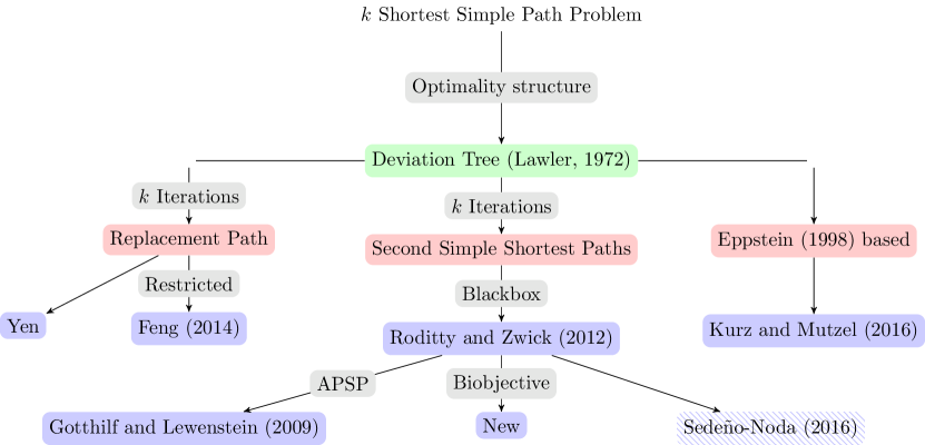
Figure 1: Relevant literature for this paper. The green node represents the optimality structure used by all algorithms to keep track of the solution paths as they are found and to avoid duplicates (see Section 2). Red nodes symbolize solution approaches. Blue nodes refer to $k$-SSP algorithms. If a blue node has solid background, the corresponding algorithm has a state of the art asymptotic running time.

To solve the $k$-SSP problem efficiently, algorithms need to keep track of the $s$-$t$-paths found so far and be able to avoid the generation of duplicates without the need to pairwise compare a new path with every existing path. All relevant $k$-SSP algorithms do so using an optimality structure called deviation tree first devised by Lawler (1972), to be discussed in Section 2. It is based on the consideration of subpaths.

Definition 2.

Given a digraph $D=(V,A)$ and a simple $u$-$w$-path $p$ in $D$ between distinct nodes $u,w\in V$, we denote a subpath of $p$ between nodes $v,v^{\prime}\in p$ by $p^{v\rightarrow v^{\prime}}$. Thereby, if $v=s$ we call $p^{v\rightarrow v^{\prime}}=p^{s\rightarrow v^{\prime}}$ a prefix of $p$ and if $v^{\prime}=t$ we call $p^{v\rightarrow v^{\prime}}=p^{v\rightarrow t}$ a suffix of $p$. For a node $v$ along $p$, we write $v\in p.$

Undoubtedly the classical $k$-SSP algorithm is due to Yen (1972). It performs $k$ iterations and starts with a solution sequence $P=(p_{1})$ containing only a shortest $s$-$t$-path $p_{1}$. In the $i$^th iteration, $i\in\{1,\dotsc,k\}$, an $i$^th shortest $s$-$t$-path $p_{i}$ is considered and the following set of $s$-$t$-paths is computed.

$$\big{\{}q\ \big{|}\ q=p_{i}^{s\rightarrow v}\circ q^{v\rightarrow t},\,q^{v\rightarrow t}\text{ shortest $v$-$t$-path in }D\setminus\{\delta^{+}(v)\cap p_{i}\},\,v\in p_{i}\big{\}}.$$ (1)

The set is a solution to the so called Replacement Path (RP) problem. The paths from this set and from all such sets computed in previous iterations are stored in a priority queue of $s$-$t$-paths from which, at the beginning of the $(i+1)$^th iteration, a $(i+1)$^th shortest path is extracted and stored in the solution sequence $P$. The simple $s$-$t$-path $p_{i}$ has at most $n$ nodes and thus, (1) contains at most $n-1$ elements, each of them requiring a shortest path computation to obtain the suffix $q^{v\rightarrow t}$. Yen’s algorithm solves the RP instances in a straightforward way iterating over the nodes in $p_{i}$ and solving the corresponding shortest path instances. Using Dijkstra’s algorithm (Dijkstra, 1959) with a Fibnoacci Heap (Fredman and Tarjan, 1987) for these queries, we obtain a running time for the solution of the RP problem of

$$T_{RP}:=\mathcal{O}\left(n(n\log{n}+m)\right).$$ (2)

The deviation tree by Lawler (1972) (also called pseudo-tree in the literature (cf. Martins and Pascoal, 2003)) is used to ensure that the solution paths for (1) computed in every iteration of Yen’s algorithm differ from each other without the need to pairwise compare them. Then, Yen’s algorithm has an asymptotic running time of

$$\mathcal{O}\left(kT_{RP}\right).$$ (3)

There is a recent alternative $k$-SSP algorithm running in $\mathcal{O}\left(kT_{RP}\right)$ that can also be considered the current state of the art and is due to Kurz and Mutzel (2016). We refer to this algorithm as the KM algorithm. Interestingly, the authors achieve this running time without solving the RP problem as a subroutine. Instead, their algorithm can be seen as a generalization of Eppstein’s algorithm (Eppstein, 1998) for the $k$-Shortest Path problem in which the output paths are allowed to contain nodes multiple times. Instead of solving One-to-One Shortest Path instances as required in (1), the KM algorithm solves One-to-All Shortest Path instances, hence obtaining a shortest path tree from every search. These instances are defined on the reversed input digraph and are rooted at the target node. The main idea of the KM algorithm, similar to the idea in (Eppstein, 1998), is that $\mathcal{O}\left(m\right)$ simple $s$-$t$-paths can be obtained from such a tree using non-tree arcs to create alternative $s$-$t$-paths. By doing so, a cycle may be constructed in which case the KM algorithm needs to compute a new shortest path tree. In addition to its state of the art running time bound, the efficiency of the KM algorithm in practice is immediately apparent: in well behaved networks, only few shortest path trees are needed since the swapping of tree arcs and non-tree arcs yield enough simple $s$-$t$-paths. Indeed, in the computational experiments conducted in (Kurz and Mutzel, 2016), the KM algorithm clearly outperforms the previous state of the art $k$-SSP algorithm by Feng (2014a). This algorithm resembles Yen’s algorithm but partitions nodes into three classes, being able to ignore nodes from one of the classes while solving (1). Due to the reduced search space/graph, the One-to-One Shortest Path computations finish faster than in Yen’s algorithm.

1.1.1 Better Asymptotics and Better Computational Performance

The algorithm by Gotthilf and Lewenstein (2009) (GL algorithm) improves the best known asymptotic running time for the $k$-SSP problem. It makes use of the All Pairs Shortest Path (APSP) algorithm introduced in Pettie (2004) to achieve an asymptotic running time bound of $\mathcal{O}\left(k(n^{2}\log{\log{n}}+nm)\right).$ Here, the term $(n^{2}\log{\log{n}}+nm)$ corresponds to the APSP running time bound derived by Pettie, while $k$ APSP instances need to be solved in the GL algorithm. As a brief digression from the main focus of the paper, we remark that a new APSP algorithm published in Orlin and Végh (2022) achieves an asymptotic running time bound of $\mathcal{O}\left(mn\right)$ for instances with nonnegative integer arc costs. Using this new algorithm as a subroutine in the GL algorithm, the following result is immediate.

Theorem 1 ($k$-SSP Running Time for Integer Arc Costs).

The $k$-SSP problem from Definition 1 with integer arc costs can be solved in $\mathcal{O}\left(kmn\right)$ time.

Despite the unbeaten asypmtotic running time bound, the GL algorithm does not perform well in practice. Solving $k$ APSP instances requires too much computational effort.

There are $k$-SSP algorithms whose asymptotic running time bound is worse than (3) and possibly not even pseudo-polynomial but that perform extremely well in practice. The current state of the art among these algorithms is published in Sedeño-Noda (2016) and in Feng (2014b), the latter publication being based on the MPS algorithm (Martins et al., 1999). Both algorithms are very different from the ones we study here and space limits detain us from discussing them in more detail.

1.2 Contribution and Outline

Figure 1 shows that there is a third approach to the $k$-SSP problem. Namely, Roditty and Zwick (2005, 2012) show that the $k$-SSP problem can be tackled by solving at most $2k$ instances of the Second Simple Shortest Path ($2$-SSP) problem. In their publications, the authors do not specify how the $2$-SSP instances arising as subproblems in their algorithm can be solved efficiently.

We design, for the first time, a computationally competitive version of the black box algorithm by Roditty and Zwick. To do so we use a novel algorithm for the $2$-SSP problem. This algorithm is based on a One-to-One version of the recently published Biobjective Dijkstra Algorithm (BDA) (Sedeño Noda and Colebrook, 2019; Maristany de las Casas et al., 2021a, b).

Algorithms that generate (shortest) paths w.r.t. a scalar arc cost function iteratively are known as ranking algorithms. These algorithms are sometimes used to solve the $k$-SSP problem (Sedeño-Noda, 2016) or to solve Biobjective Shortest Path (BOSP) instances hoping that the generated paths are optimal in the given biobjective setting (cf. Martins et al., 1999). Ranking approaches to solve BOSP problems seem nowadays outdated given the improved efficiency reached by recent algorithms (Sedeño Noda and Colebrook, 2019; Ahmadi et al., 2021; Maristany de las Casas et al., 2023). Our approach of solving $2$-SSP instances by defining a BOSP instance and solving it using the BDA turns around the strategies used so far: the $k$-SSP problem, suitable for ranking algorithms, is solved solving $\mathcal{O}\left(k\right)$ BOSP instances as subroutines.

In Section 2 we describe the deviation tree, the optimality structure used throughout the chapter. In Section 3 we discuss our main contribution: a new $2$-SSP algorithm using a biobjective approach. Even if it might sound counter-intuitive to define a biobjective subroutine for an optimization problem with scalar costs, its running time matches the running time bound (2). In Section 4 we describe the $k$-SSP algorithm by Roditty and Zwick (2012) that solves $\mathcal{O}\left(k\right)$ $2$-SSP instances. In the final Section 5 we demonstrate the efficiency of our algorithm in practice, benchmarking it against the KM algorithm (Kurz and Mutzel, 2016).

2 Optimality Structure – Deviation Tree

Consider a $k$-SSP instance $\mathcal{I}:=(D,s,t,c,k)$. A (partial) solution sequence $P_{\ell}=(p_{1},\dotsc,p_{\ell})$ for $\ell\in[1,k]$ is represented as a deviation tree $T_{P_{\ell}}$ (e.g., Lawler, 1972; Martins and Pascoal, 2003; Roditty and Zwick, 2012). $T_{P_{\ell}}$ is a directed graph, represented as a tree in which a node from the original graph $D$ may appear multiple times. The root node of $T_{P_{\ell}}$ is a copy of the node $s$ in $D$ and every leaf corresponds to a copy of the node $t$. There are $\ell$ leafs and any path from the root to a leaf is in one-to-one correspondence with an $s$-$t$-path in $D$.

Definition 3 (Deviation Tree.).

The deviation tree $T_{P_{\ell}}$ is built iteratively. Initially, $T_{P_{\ell}}$ is empty. $p_{1}$ is added to $T_{P_{\ell}}$ by adding all nodes and edges of $p_{1}$ to the tree. For any $j\in[2,\ell]$, assume that the previous paths $p_{i}$, $i\in[1,j)$ have been added to $T_{P_{\ell}}$ already. Assume the longest common prefix of $p_{j}$ with a path $p_{i}\in P_{j-1}$ is the $s$-$v$-subpath $p_{j}^{s\rightarrow v}$ for a $v\in p_{j}$. Then, $p_{j}$ is added to $T_{P_{\ell}}$ by appending the suffix $p_{j}^{v\rightarrow t}$ of $p_{j}$ to the copy of $v$ along $p_{i}$ in $T_{P_{\ell}}$.

Parent Path

The path $p_{1}$ has no parent path. For any path $p_{i}$, $i\in\{2,\dotsc,\ell\}$, the parent path $p$ is the path in $P_{\ell}$ with which $p_{i}$ shares the longest (w.r.t. the number of arcs) common prefix $p_{i}^{s\rightarrow v}$. In case $p$ is not uniquely defined, $p$ is set to be the first path in $P_{\ell}$ with $p^{s\rightarrow v}=p_{i}^{s\rightarrow v}$. If $p$ is the parent path of $p_{i}$, $p_{i}$ is a child path of $p$.

Deviation Arc, Deviation Node, Source Node

The path $p_{1}$ has no deviation arc, its deviation node is $s$ and it its source node is also $s$. For any path $p_{i}$, $i\in\{2,\dotsc,\ell\}$ the deviation arc is the first arc $(v,w)$ along $p_{i}$ after the common prefix of $p_{i}$ with its parent path. The node $v$ is called the deviation node of $p_{i}$ and the node $w$ is called the source node of $p_{i}$. For any path $p\in P_{\ell}$ we write $\mathtt{dev}(p)$ and $\mathtt{source}(p)$ to refer to these nodes.

Recall that we assume the paths in $P_{\ell}$ to be sorted non-decreasingly according to their costs. Then, the parent path $p$ of any path $q\in P_{\ell}$ is stored before $q$ in $P_{\ell}$ and we have $c(p)\leq c(q)$. Moreover, the inductive nature of $T_{P_{\ell}}$ guarantees that the deviation node of $p$ does not come after the deviation node of $q$.

Example 1.

The left hand side of Figure 2 shows a $4$-SSP instance. We set $P=(p_{1},\dotsc,p_{4})$ with $p_{1}=((s,v),(v,t))$, $p_{2}=((s,u),(u,t))$, $p_{3}=((s,w),(w,t))$, and $p_{4}=((s,u),(u,v),(v,t))$. The right hand side depicts the deviation tree $T_{P}$ as defined in Definition 3. When building $T_{P}$ iteratively, $p_{1}$ is added first. Then, the longest common prefix of $p_{1}$ and $p_{2}$ is identified to be just the node $s$. Thus, $p_{2}$ is appended to $s$ in $T_{P}$. The parent path of $p_{2}$ is $p_{1}$, the deviation node is $s$, and the source node is $u$. Adding $p_{3}$ to $T_{P}$ leads to the situation in which two paths, namely $p_{1}$ and $p_{2}$, share the longest common prefix with $p_{3}$: the node $s$ only. Hence, the parent path of $p_{3}$ is set by definition to be $p_{1}$, the first path in $P$ sharing the longest common prefix with $p_{3}$. $p_{3}$’s deviation node is $s$ and its source node is $w$. Finally, the path $p_{4}$ is added to $T_{P}$. It shares its prefix $p_{4}^{s\rightarrow u}$ of maximum length with $p_{2}$ and thus its suffix $p_{4}^{u\rightarrow t}=((u,v),(v,t))$ is appended in $T_{P}$ to the copy of the node $u$ along $p_{2}$ in $T_{P}$. The deviation node of $p_{4}$ is $u$ and its source node is $v$.

Figure 2: Left: Input graph $D$ and arc costs for a $k$-SSP instance. Right: Pseudo-Tree $T_{P}$ corresponding to the $k$-SSP instance defined on the left with $k=4$.

3 Second Shortest Simple Path Problem

We introduce a new $2$-SSP algorithm. Assuming that a shortest path $p$ is known, we define a biobjective arc cost function $\gamma_{p}:A\to\mathbb{R}^{2}$ depending on $p$ that allows us to find a second shortest path as the first or the second (in lexicographic order w.r.t. $\gamma$) efficient solution of a One-to-One Biobjective Shortest Path (BOSP) instance associated with $p$.

Definition 4.

Consider a digraph $D=(V,A)$, nodes $s,\,t\in V$, and an arc cost function $c:A\to\mathbb{R}_{\geq 0}$. $\mathcal{I}=(D,s,t,c)$ is an instance of the classical One-to-One Shortest Path problem. Let $p$ be a shortest $s$-$t$-path in $D$. For every arc $a\in A$ define two dimensional costs $\gamma_{p}(a)\in\mathbb{R}_{\geq 0}^{2}$ setting $\gamma_{p,1}(a)=c(a)$ and $\gamma_{p,2}(a)=1$ if $a\in p$. Otherwise, set $\gamma_{p,2}(a)=0$. The BOSP instance $\mathcal{I}_{\text{BOSP}}^{p}=(D,s,t,\gamma_{p})$ is the BOSP instance associated with $\mathcal{I}$ and $p$.

Initially, using a biobjective subroutine in an optimization problem with scalar cost sounds counter-intuitive. The reasons are intractability of the Biobjective Shortest Path problem (cf. Hansen, 1980) and the consequent time and memory demands.However, the $\gamma_{p}$ function defined in Definition 4 is such that at most $n-1$ $s$-$t$-paths are optimal (cf. Lemma 1) making the $\mathcal{I}_{\text{BOSP}}^{p}$ instances tractable. Moreover, the $\{0$,$1\}$ second component of $\gamma_{p}$ plays an essential role to circumvent the issue of second shortest paths not adhering to the subpath-optimality principle as explained in the following example.

Example 2.

Consider the $\mathcal{I}_{\text{BOSP}}^{p}$ instance defined in Figure 3 w.r.t. the shortest $s$-$t$-path $p$ in that instance. The shown graph contains two $s$-$v_{4}$-paths:

$$\begin{split}q=((s,v_{1}),(v_{1},v_{4}))\text{ with }c(q)=\gamma_{p,1}(q)=2\\ r=((s,v_{1}),(v_{1},v_{2}),(v_{2},v_{3}),(v_{3},v_{4}))\text{ with }c(r)=\gamma_{p,1}(r)=1\end{split}$$

A decision made based on these costs favors the path $r$ since $c(r)<c(q)$. However, the extension of $r$ towards $v_{2}$ produces a cycle, causing any expansion of $r$ to be an invalid candidate for a second shortest simple $s$-$t$-path. Thus, when comparing $q$ and $r$ both paths need to be recognized as promising candidates. Since $q$ shares only one arc with $p$ before it deviates, we have $\gamma_{p,2}(q)=1$. For the same reason, we have $\gamma_{p,2}(r)=3$. Thus, $\gamma_{p}(q)=(2,1)$ and $\gamma_{p}(r)=(1,3)$ and both paths are efficient/optimal $s$-$v_{4}$-paths in our biobjective setting.

Note that $v_{2}$ is already visited by $r$’s subpath $r^{s\rightarrow v_{2}}$ with cost $\gamma_{p}(r^{s\rightarrow v_{2}})=(0,2)$. After expanding $q$ and $r$ along the arc $(v_{4},v_{2})$, we have $\gamma_{p}(q\circ(v_{4},v_{2}))=(4,1)$ and $\gamma_{p}(r\circ(v_{4},v_{2}))=(3,3)$ and we see that $r$’s expansion is dominated by $r^{s\rightarrow v_{2}}$ and thus can be discarded. $q$’s expansion on the other side is not dominated and thus, the bad $s$-$v_{4}$-path w.r.t. the original cost function $c$ is kept to build a simple second shortest $s$-$t$-path.

Figure 3: $\mathcal{I}_{\text{BOSP}}^{p}$ instance for the shortest path $p=((s,v_{1}),(v_{1},v_{2}),(v_{2},v_{3}),(v_{3},t))$. The red arcs show a $s$-$v_{2}$-path that is not simple. Its $s$-$v_{4}$-subpath is the shortest $s$-$v_{4}$-path w.r.t. the original arc costs $c=\gamma_{1}$.

The $\gamma$ arc cost function not only elevates the status of paths with suboptimal subpaths w.r.t. $c$ to become efficient paths in the $\mathcal{I}_{\text{BOSP}}$ instances. We can additionally use a technique called dimensionality reduction that allows dominance tests in biobjective optimization problems to be done in constant time. Since, as in the last example, paths that are not simple will turn out to be dominated, we manage to detect cycles without hashing a path’s nodes.

The BOSP algorithm to solve the $\mathcal{I}_{\text{BOSP}}$ instances must be chosen carefully to obtain a competitive running time bound for our $k$-SSP algorithm in Section 4.

3.1 Biobjective Dijkstra Algorithm

The One-to-One Biobjective Dijkstra Algorithm (BDA) (Sedeño Noda and Colebrook, 2019; Maristany de las Casas et al., 2021a, b) is a BOSP algorithm that features the currently best theoretical output sensitive running time bound known for this problem. As the name suggests, it proceeds similarly to Dijkstra’s algorithm (Dijkstra, 1959) for the classical Shortest Path problem. It uses a priority queue in which paths are sorted in lexicographically (lex.) nondecreasing order w.r.t. $\gamma$. While in Dijkstra’s algorithm the queue only needs to store the cheapest known $s$-$v$-path for every node $v\in V$, BOSP algorithms prior to the BDA needed to be able to handle multiple $s$-$v$-paths. All explored $s$-$v$-paths that are not dominated by and not cost-equivalent to already stored $s$-$v$-paths need to be stored; here, a path $p$ is said to dominate a path $q$ if $\gamma_{i}(p)\leq\gamma_{i}(q)$ for $i\in\{1,2\}$ and one of the inequalities is strict. After an $s$-$v$-path for some $v\in V$ is extracted from the queue, it is stored in the list of optimal $s$-$v$-paths $P^{*}_{sv}$ and propagated along the outgoing arcs of $v$ to obtain new candidate $s$-$w$-paths, $(v,w)\in\delta^{+}(v)$. In the biobjective optimization literature, and also hereinafter, optimal solutions are called efficient. The BDA returns a minimum complete set of efficient paths. This means that if for a non-dominated cost vector $c$ there are multiple efficient $s$-$t$-paths $p$ with $\gamma(p)=c$, the BDA returns just one of these paths.

The main idea in the design of the BDA is that biobjective shortest paths adhere to a dynamic programming principle: the efficient $s$-$v$-paths can be build out of the optimal $s$-$u$-paths for $u\in\delta^{-}(v)$. Exploiting this principle, the BDA manages to store just the lex-smallest non-dominated $s$-$v$-path in its queue. When this path is extracted from the queue and stored in the corresponding list $P^{*}_{sv}$ of efficient paths, it rebuilds the next candidate $s$-$v$-path looking at the efficient $s$-$u$-paths in $P^{*}_{su}$ for $(u,v)\in\delta^{-}(v)$. Thanks to this idea, we obtain the following running time and space consumption bound:

Theorem 2.

Let $\mathcal{I}=(D,s,t,\gamma)$ be a BOSP instance and set $N_{\max}:=\max_{v\in V}|P^{*}_{sv}|$ and $N=\sum_{v\in V}|P^{*}_{sv}|$. The BDA runs in $\mathcal{O}\left(N\log{n}+N_{\max}m\right)$ time and uses $\mathcal{O}\left(N+n+m\right)$ space.

For further details regarding the (One-to-One) BDA, we refer to the original publications (Sedeño Noda and Colebrook, 2019; Maristany de las Casas et al., 2021b). A detailed discussion of the running time and space consumption bounds for the BDA and other BOSP algorithms can be found in Maristany de las Casas et al. (2021a).

3.2 Second Simple Shortest Paths Using the BDA

We formulate the following main result in this section.

Theorem 3.

Consider a shortest path problem $\mathcal{I}=(D,s,t,c)$, let $p$ be a shortest $s$-$t$-path w.r.t. $c$ and assume it has $\ell$ arcs. A lexicographically smallest (w.r.t. $\gamma_{p}$) efficient $s$-$t$-path $q$ with $\gamma_{p,2}(q)<\ell$ in the BOSP instance $\mathcal{I}_{\text{BOSP}}^{p}$ is a second shortest simple $s$-$t$-path in $D$ w.r.t. the original costs $c$.

Proof.

We assume that $\mathcal{I}_{\text{BOSP}}^{p}$ is solved using the BDA. Every efficient path in this instance is a simple path or cost-equivalent to a simple path since $\gamma_{p}$ is a non-negative function. Additionally, efficient paths containing a loop are neither made permanent nor further expanded by the BDA since the algorithm uses the reflexive $\preceq_{D}$-operator. As a consequence, every path $q$ that is made permanent fulfills $\gamma_{p,2}(q)\leq\ell$ and the only possibly extracted path with $\gamma_{p,2}(q)=\ell$ is $p$ with costs $\gamma_{p}(p)=(c(p),\ell)$.

Since $p$ is a shortest $s$-$t$-path, any extracted $s$-$t$-path $q\neq p$ fulfills $\gamma_{p,1}(q)\geq\gamma_{p,1}(p)$. Thus, if $q$ is made permanent before $p$, it is lex-smaller than $p$ and we must have $\gamma_{p,1}(q)=\gamma_{p,1}(p)$ and $\gamma_{p,2}(q)<\gamma_{p,2}(p)$. The second inequality implies that $q$ and $p$ are distinct paths and we thus can stop the execution of the BDA and return $q$ as a second shortest simple $s$-$t$-path. In this case, $p$ and $q$ are cost-equivalent w.r.t. $c$.

Assume $p$ is permanent already and $q$ is the next $s$-$t$-path extracted from the BDA’s priority queue. We must have $\gamma_{p,1}(p)<\gamma_{p,1}(q)$ (see last paragraph). Recall that the BDA finds a minimum complete set of efficient paths for $\mathcal{I}_{\text{BOSP}}^{p}$. Moreover, as already noted, paths are extracted from the algorithm’s priority queue in lex. nondecreasing order. Thus, since efficient paths are simple, we conclude that there cannot exist a simple $s$-$t$-path $q^{\prime}$ with $\gamma_{p,1}(p)\leq\gamma_{p,1}(q^{\prime})<\gamma_{p,1}(q)$ that is not found by the BDA. Since the $\gamma_{p,1}$ costs are equivalent to the original $c$ costs of the paths in $D$, we obtain that $q$ is a second shortest simple $s$-$t$-path. ∎

The shortest path $p$ is the only simple path in $\mathcal{I}_{\text{BOSP}}^{p}$ with $\gamma_{2}(p)=\ell$. Since we want to find an efficient $s$-$t$-path $q$ with $\gamma_{p,2}(q)<\ell$, the BDA can stop after at most two $s$-$t$-paths are extracted from the priority queue: the path $p$ that is efficient iff $\gamma_{p,1}(p)<\gamma_{p,1}(q)$ and $q$ itself. Using this stopping criterion, we define the following modified version of the BDA as our new $2$-SSP algorithm.

Definition 5 ($\text{BDA}_{2\text{SSP}}$).

The $\text{BDA}_{2\text{SSP}}$ is a $2$-SSP algorithm. It modifies the BDA as follows.

Input

In addition to a BOSP instance, the input of the $\text{BDA}_{2\text{SSP}}$ contains a non-negative integer $\ell$.

Stopping Condition

The $\text{BDA}_{2\text{SSP}}$ stops whenever an efficient $s$-$t$-path $q$ with $\gamma_{p,2}(q)<\ell$ is extracted from the priority queue or when the priority queue is empty at the beginning of an iteration.

Output

Instead of a minimum complete set of efficient $s$-$t$-paths, the new $\text{BDA}_{2\text{SSP}}$ returns the suffix $q^{v\rightarrow t}$ of the first efficient $s$-$t$-path $q$ with $\gamma_{p,2}(q)<\ell$ that it finds. Here, $v$ is the node after which $p$ and $q$ deviate for the first time. If such a path $q$ does not exist, the $\text{BDA}_{2\text{SSP}}$ returns a dummy path if such a path does not exist.

3.3 Asymptotic Running Time and Memory Consumption

The following is a general statement that holds for any biobjective optimization problem (cf. Jochen Gorski and Sudhoff, 2023).

Lemma 1.

Let $\mathcal{X}$ be the set of feasible solutions of a biobjective optimization problem and $f:\mathcal{X}\to\mathbb{R}_{\geq 0}\times\mathbb{N}$ the associated cost function. The cardinality of a minimum complete set of efficient solutions is bounded by the size of the set $\{f_{2}(x)\ |\ x\in\mathcal{X}\}$.

Proof.

Assume for a value $y_{2}\in\{f_{2}(x)\ |\ x\in\mathcal{X}\}$ there are two efficient solutions $x$, $x^{\prime}$ in a minimum complete set. If $f_{1}(x)\neq f_{1}(x^{\prime})$, then the solution with the smaller $f_{1}$ value (weakly) dominates the other. If $f_{1}(x)=f_{1}(x^{\prime})$, both solutions are cost-equivalent and, by definition, no minimum complete set contains both. ∎

Our setting in this section assumes a shortest $s$-$t$-path $p$ with $\ell$ arcs to be given and we look for a second shortest $s$-$t$-path in the same graph. In the first paragraph of the proof of Theorem 3 we derived that any efficient path $q$ for the instance $\mathcal{I}_{\text{BOSP}}^{p}$ fulfills $\gamma_{p,2}(q)\leq\ell$. Lemma 1 applied to $\mathcal{I}_{\text{BOSP}}^{p}$ implies that every minimum complete set of efficient $s$-$v$-paths, $v\in V$, has cardinality at most $\ell$.

For the set of efficient $s$-$t$-paths computed by the $\text{BDA}_{2\text{SSP}}$ we even now that it contains at most two paths at the end of the algorithm. Sadly, we cannot mirror this fact in the running time bound for the $\text{BDA}_{2\text{SSP}}$. As explained in Bökler (2018) and Maristany de las Casas et al. (2023) for a One-to-One BOSP instance, a minimum complete set of efficient $s$-$t$-paths can contain less paths than the number of efficient $s$-$v$-paths calculated for an intermediate node $v$. Thus, even though it calculates at most two $s$-$t$-paths, the $\text{BDA}_{2\text{SSP}}$ may compute $\ell-1$ (not $\ell$ because $s$-$t$-paths are not propagated) $s$-$v$-paths for an intermediate node $v$. Using the running time bound of the BDA described in Theorem 2, we obtain the following result.

Theorem 4.

The $\text{BDA}_{2\text{SSP}}$ solves a $2$-SSP instance $\mathcal{I}:=(D,s,t,c,2)$ in time

$$\mathcal{O}\left(n\ell\log{n}+\ell m\right)=\mathcal{O}\left(\ell(n\log{n}+m)\right)\in\mathcal{O}\left(n(n\log{n}+m)\right).$$ (4)

Based on the memory consumption derived for the BDA in Theorem 2, we conclude this section stating the space consumption bound of the $\text{BDA}_{2\text{SSP}}$.

Theorem 5.

The $\text{BDA}_{2\text{SSP}}$ uses

$$\mathcal{O}\left(n\ell+n+m\right)\in\mathcal{O}\left(n^{2}+n+m\right)\in\mathcal{O}\left(n^{2}+m\right)$$ (5)

memory.

Proof.

The original version of the BDA uses $\mathcal{O}\left(N+n+m\right)$ space where $N=\sum_{v\in V}N_{v}$ and $N_{v}$ is the number of efficient $s$-$v$-paths calculated by the algorithm. We have $N\leq nN_{\max}$ with $N_{\max}=\max_{v\in V}N_{v}$ and in our $\text{BDA}_{2\text{SSP}}$ scenario $N_{\max}<\ell$ as discussed already. The modifications defined in Definition 5 to the original BDA to obtain the $\text{BDA}_{2\text{SSP}}$ do not have any further impact on the space consumption. ∎

3.4 Properties of the Second Shortest Simple Path Problem

In this section we discuss three structural properties of the $2$-SSP problem. They are helpful for the description of our new $k$-SSP algorithm introduced in Section 4. Note that whenever we remove a path $p$ from a given digraph $D$, we write $D\setminus p$ and we delete the nodes and the arcs of $p$ from $D$.

The following easy statement is essential for the understanding of the remainder of the chapter. The proof follows directly from Definition 3.

Lemma 2.

Consider a $2$-SSP instance and let $P=(p_{1},p_{2})$ be a solution sequence with associated deviation tree $T_{P}$. Then, $p_{1}$ is the parent path of $p_{2}$.

Lemma 3.

Consider a $2$-SSP instance $\mathcal{I}:=(D,s,t,c,2)$ and let $P=(p_{1},p_{2})$ be a solution sequence. Assume that $(v,w)$ is $p_{2}$’s deviation arc which is well defined due to Lemma 2. The suffix path $p_{2}^{w\rightarrow t}$ is a shortest $w$-$t$-path in the digraph $D\setminus p_{2}^{s\rightarrow v}$.

Proof.

We can write $p_{2}=p_{1}^{s\rightarrow v}\circ(v,w)\circ p_{2}^{w\rightarrow t}$. If a $w$-$t$-path $q^{w\rightarrow t}$ with $c(q^{w\rightarrow t})<c(p_{2}^{w\rightarrow t})$ exists in $D\setminus p_{2}^{s\rightarrow v}$ we have $c(p_{2})>c(p_{1}^{s\rightarrow v}\circ(v,w)\circ q^{w\rightarrow t})$ and $p_{2}$ would not be a second shortest $s$-$t$-path in $D$. ∎

As a consequence of the last lemma, we formulate the following result.

Corollary 1.

A second simple shortest path is given by

$$\begin{split}p_{2}:=\operatorname*{arg\,min}\Big{\{}c(q)\ \Big{|}\ &q=p_{1}^{s\rightarrow v}\circ(v,w)\circ q^{w\rightarrow t},\,\\ &q^{w\rightarrow t}\text{ shortest }\text{$w$-$t$-path in }D\setminus p_{1}^{s\rightarrow v},\,\\ &(v,w)\in\delta^{+}(v)\setminus p_{1},\,v\in p_{1}\Big{\}}.\end{split}$$ (6)

We observe that the solution $p_{2}$ in (6) is contained in the solution set (1) of a Replacement Path (RP) instance. Thus, in a worst case scenario, the $\text{BDA}_{2\text{SSP}}$ needs to do as much effort as an RP algorithm to find $p_{2}$ in the set (1) of RP solutions. This intuition is formally mirrored in Williams and Williams (2018, Theorem 1.1). The result states that while currently having the same complexity, a truly subcubic $2$-SSP algorithm implies a truly subcubic RP algorithm. I.e., it is unlikely to design an algorithm solving $2$-SSP instances faster than RP instances in the worst case.

However, for practical purposes the fact that the solution $p_{2}$ from (6) is included in the set (1) unveils the strength of the $\text{BDA}_{2\text{SSP}}$ as a $2$-SSP algorithm: stopping after at most two paths reach the target node $t$ reduces the number of iterations in comparison to the need to solve $\mathcal{O}\left(n\right)$ One-to-One Shortest Path instances to calculate (1).

4 K-SPP Algorithm by Roditty and Zwick using the BDA

Roditty and Zwick (2012) discuss a black box algorithm for the $k$-SSP problem. It is a black box algorithm because the authors do not specify how to solve the key subroutine in their algorithm: the computation of a second-shortest simple path. Moreover, they do not implement their algorithm in the paper. In this section we fill the gap using the $\text{BDA}_{2\text{SSP}}$.

The algorithm presented in (Roditty and Zwick, 2012) performs $2k$ computations of a second shortest simple path to solve a $k$-SSP instance $\mathcal{I}:=(D,s,t,c,k)$. It fills the solution sequence $P$ iteratively. In our exposition we assume that at any stage, the deviation tree $T_{P}$ associated with $P$ exists implicitly. In particular, this allows us to use the notions from Definition 3. We discuss this in detail in Remark 2. The pseudocode for our new algorithm is in Algorithm 1.

Remark 1 (Source nodes in $\mathcal{I}_{\text{BOSP}}$ instances).

Given an $\ell$^th shortest path $p_{\ell}$ for some $\ell\in\{1,\dotsc,k\}$, the corresponding BOSP instance $\mathcal{I}_{\text{BOSP}}^{p_{\ell}}$ is defined as in Definition 4 but the source node in $\mathcal{I}_{\text{BOSP}}^{p_{\ell}}$ is not always the actual source node $s$ of our $k$-SSP instance. For $\mathcal{I}_{\text{BOSP}}^{p_{\ell}}$ the source node is $\mathtt{source}(p_{\ell})$. Despite being important for the correctness of Algorithm 1, this makes sense because in Definition 4 we assume a shortest path to be given. As discussed in the previous section, the $\ell$^th shortest path $p_{\ell}$ in the original graph $D$ is not a shortest $s$-$t$-path but its suffix $p_{\ell}^{\mathtt{source}(p_{\ell})\rightarrow t}$ is a shortest path in a modified version of $D$.

Input : $k$-SSP instance $\mathcal{I}:=(D,s,t,c,k)$

Output : Solution sequence $P=(p_{1},\dotsc,p_{k})$ of distinct simple $s$-$t$-paths.

1 Priority queue of candidate $s$-$t$-paths $C\leftarrow\emptyset$;

2 $p_{1}\leftarrow$ shortest $s$-$t$-path in $D$;

3 Solution sequence $P\leftarrow(p_{1})$;

4 $p_{2}\leftarrow$ $\text{BDA}_{2\text{SSP}}$ solution for $\mathcal{I}_{\text{BOSP}}^{p_{1}}$;

5 $(v,w)\leftarrow$ Parent deviation arc of $p_{2}$;

6 Add $(v,w)$ to $\mathtt{blocked}(p_{1})$;

7 Insert $p_{2}$ to $C$;

8 for $\ell\in\{2,\dotsc,k\}$ do

9       $p_{\ell}\leftarrow$ Extract path from $C$ with min. costs;

10       Add $p_{\ell}$ to the solution sequence $P$;

11       if $\ell==k$ then break;

12       $q^{\mathtt{source}(p_{\ell})\rightarrow t}\leftarrow$ $\text{BDA}_{2\text{SSP}}$ solution for $\mathcal{I}_{\text{BOSP}}^{p_{\ell}}=(\bar{D},\mathtt{source}(p_{\ell}),t,\gamma_{p_{\ell}})$ with $\bar{D}=D\setminus p_{\ell}^{s\rightarrow\mathtt{dev}(p_{\ell})}$;

13       if $q^{\mathtt{source}(p_{\ell})\rightarrow t}\neq NULL$ then

14             New $s$-$t$-path $q\leftarrow p_{\ell}^{s\rightarrow\mathtt{source}(p_{\ell})}\circ q^{\mathtt{source}(p_{\ell})\rightarrow t}$;

15             $(v^{\prime},w^{\prime})\leftarrow$ Parent deviation arc of $q$;

16             Add $(v^{\prime},w^{\prime})$ to $\mathtt{blocked}(p_{\ell})$;

17             Insert $q$ into $C$;

18            

19      $p\leftarrow$ Parent path of $p_{\ell}$;

20       $q^{\mathtt{source}(p)\rightarrow t}\leftarrow$ $\text{BDA}_{2\text{SSP}}$ solution for $\mathcal{I}_{\text{BOSP}}^{p}=(\bar{D},\mathtt{source}(p),t,\gamma_{p})$ with $\bar{D}=D\backslash(p^{s\rightarrow\mathtt{dev}(p)}\cup\mathtt{blocked}(p))$;

21       if $q^{\mathtt{source}(p)\rightarrow t}\neq NULL$ then

22             New $s$-$t$-path $q\leftarrow p^{s\rightarrow\mathtt{source}(p)}\circ q^{\mathtt{source}(p)\rightarrow t}$;

23             $(v^{\prime},w^{\prime})\leftarrow$ deviation arc of $q$;

24             Add $(v^{\prime},w^{\prime})$ to $\mathtt{blocked}(p)$;

25             Insert $q$ into $C$;

26            

27return $P$;

Algorithm 1 New algorithm for the $k$-SSP problem.

The global data structures of the algorithm are the solution sequence $P$ and a priority queue $C$ of $s$-$t$-paths sorted according to the paths’ costs. Both structures are initially empty. In its initialization phase, the algorithm computes a shortest $s$-$t$-path $p_{1}$ in $D$ w.r.t $c$ and stores it in $P$ as the first solution in the solution sequence (Algorithm 1 and Algorithm 1). Additionally, a second shortest path $p_{2}$ is computed applying the $\text{BDA}_{2\text{SSP}}$ to the $\mathcal{I}_{\text{BOSP}}^{p_{1}}$ instance (Algorithm 1). The obtained path is inserted into $C$ (Algorithm 1). By Lemma 2 $p_{1}$ is the parent path of $p_{2}$. Every path in $P$ has a list of blocked arcs associated with it. For a path $p$, the list $\mathtt{blocked}(p)$ contains the deviation arcs from $p$’s children paths that are already computed. When looking for further deviations from $p$, we delete the arcs in $\mathtt{blocked}(p)$ from the digraph to ensure that the deviations leading to the already computed children paths of $p$ are not computed again. Thus, since $p_{2}$ is a child path of $p_{1}$, the $p_{2}$’s deviation arc is added to $\mathtt{blocked}(p_{1})$ (Algorithm 1).

After the initialization, the main loop of the algorithm with $k-1$ iterations starts. Every iteration $\ell\in[2,k]$ starts with the extraction of a minimal path from $C$ (Algorithm 1), which we call $p_{\ell}$. $p_{\ell}$ is immediately added to $P$ after its extraction and it becomes part of the final solution sequence (Algorithm 1).

First $\text{BDA}_{2\text{SSP}}$ calculation

Let $(v,w)=(\mathtt{dev}(p_{\ell}),\mathtt{source}(p_{\ell}))$ be the deviation arc from $p_{\ell}$ as defined in Definition 3. Then, we build the instance $\mathcal{I}_{\text{BOSP}}^{p_{\ell}}=(\bar{D},w,t,\gamma_{p_{\ell}})$ with $\bar{D}=D\setminus p_{\ell}^{s\rightarrow v}$. Recall that by Lemma 3, the suffix $p_{\ell}^{w\rightarrow t}$ is a shortest $w$-$t$-path in $\bar{D}$. Using the $\text{BDA}_{2\text{SSP}}$, a second shortest $w$-$t$-path $q^{w\rightarrow t}$ in $\bar{D}$ w.r.t. $\gamma_{p_{\ell}}$ is searched. The result, if it exists, is a new suffix for the prefix $p_{\ell}^{s\rightarrow w}$. Together, both subpaths build a new candidate $s$-$t$-path $q:=p_{\ell}^{s\rightarrow w}\circ q^{w\rightarrow t}$.

Postprocessing

If $q$ is successfully built, $p_{\ell}$ is its parent path (see Remark 2). Moreover, $q$’s deviation arc is added to the list $\mathtt{blocked}(p_{\ell})$. Finally, $q$ is added to $C$.

Second $\text{BDA}_{2\text{SSP}}$ calculation

The second $\text{BDA}_{2\text{SSP}}$ query (Algorithm 1) in every iteration looks for the next-cheapest deviation from the parent path $p$ of the extracted path $p_{\ell}$. When building the corresponding $2$-SSP instance $\mathcal{I}_{\text{BOSP}}^{p}$, the deviation arcs from $p$’s children paths must be deleted from the digraph $D$. Otherwise, the solution to $\mathcal{I}_{\text{BOSP}}^{p}$ would be an already computed deviation. Apart from deleting the arcs in $\mathtt{blocked}(p)$ from $D$, we again delete $p$’s prefix $p^{s\rightarrow\mathtt{dev}(p)}$ from $p$. This ensures that after the $\text{BDA}_{2\text{SSP}}$ computation, the concatenation of $p^{s\rightarrow\mathtt{source}(p)}$, where $w$ is the adjacent node to $v$ in $p$, and the result $q^{w\rightarrow t}$ is a simple path. If $q$ is successfully built, the algorithm repeats the postprocessing of the first $\text{BDA}_{2\text{SSP}}$ computation. This query search for the cheapest simple path alternative for $p^{w\rightarrow t}$ without considering the alternatives that have already been computed.

4.1 Correctness and Complexity

In this subsection we sketch the correctness proof and the complexity of Algorithm 1. The correctness of Algorithm 1 using a black box algorithm to solve the arising $2$-SSP instances is discussed in Roditty and Zwick (2012).

In Algorithm 1 we use the parent-child relationship of paths introduced in Definition 3. Formally we would need a proof to show that indeed the computed paths and our usage of this notion in the algorithm are in accordance with the original definition. The following remark gives a strong intuition. The proof can then easily be concluded with an induction step.

Remark 2.

We know from Lemma 2 that $p_{2}$’s parent path is $p_{1}$. In the first iteration of Algorithm 1, we thus build a $\mathtt{source}(p_{2})$-$t$-path $q^{\mathtt{source}(p_{2})\rightarrow t}$ in Algorithm 1. It is used to build an $s$-$t$-path $q:=p_{2}^{s\rightarrow\mathtt{source}(p_{2})}\circ q^{\mathtt{source}(p_{2})\rightarrow t}$. Since by definition $\mathtt{source}(p_{2})\in p_{2}$ and $\mathtt{source}(p_{2})\notin p_{1}$, $q$ shares a prefix of maximum length with $p_{2}$. Hence, $p_{2}$ induced the BOSP instance $\mathcal{I}_{\text{BOSP}}^{p_{2}}$ that led to $q$’s computation and $p_{2}$ is $q$’s parent path.

In the second $\text{BDA}_{2\text{SSP}}$ query in the first iteration, an $s$-$t$-path $q$ is computed in Algorithm 1. $q$ already starts at $s$ because $s=\mathtt{source}(p_{1})$ and thus $s$ is the source node in $\mathcal{I}_{\text{BOSP}}^{p_{1}}$ (cf. Remark 1). In the corresponding digraph, the arcs in $\mathtt{blocked}(p_{1})$ are deleted. At this stage, the list only contains $p_{2}$’s deviation arc $(v,w)=(\mathtt{dev}(p_{2}),\mathtt{source}(p_{2}))$ that was added to the list in Algorithm 1. Hence, if $q^{s\rightarrow\mathtt{dev}(q)}$ coincides with $p_{1}$ until a node $\mathtt{dev}(q)$ that comes after $\mathtt{dev}(p_{2})$ along $p_{1}$, $q$ shares a prefix of maximum length with $p_{1}$. Otherwise, if $\mathtt{dev}(q)$ does not come after $\mathtt{dev}(p_{2})$ along $p_{1}$, $q$ shares a prefix of maximum length with $p_{1}$ and $p_{2}$. By definition, the parent path of $q$ is then set to be the first of these two paths in $P$, i.e., $p_{1}$.

Recall that a child’s deviation node does not come before its parent’s deviation node as remarked already in Section 2. Then, we repeat the arguments from the last paragraphs for any path extracted from $C$ in Algorithm 1 of Algorithm 1 to proof that the notions from Definition 3 are correctly used in Algorithm 1.

The Algorithm 1 requires the deletion of prefixes from the digraph to ensure that it can generate distinct paths when concatenating the suffixes build by the $\text{BDA}_{2\text{SSP}}$ with the corresponding prefix in the parent path (see Lemma 5). Moreover, deleting the prefixes in the graphs $\bar{D}$ used by the $\text{BDA}_{2\text{SSP}}$ ensures that prefix nodes do not appear in the paths obtained from the $\text{BDA}_{2\text{SSP}}$.

Lemma 4.

Let $p$ be an $s$-$t$-path in the solution sequence $P$ of Algorithm 1 with deviation node $v$ and deviation arc $(v,w)$. Let $q^{w\rightarrow t}$ be a second shortest path computed in Algorithm 1 or in Algorithm 1. The $s$-$t$-path $q=p^{s\rightarrow w}\circ q^{w\rightarrow t}$ is simple.

Proof.

For the computation of $q^{w\rightarrow t}$, we delete the prefix $p^{s\rightarrow v}$ from $D$ to build $\bar{D}$. Hence, both subpaths are node-disjoint. As discussed already, the non-negativity of every $\gamma$ ensures that the path output by the $\text{BDA}_{2\text{SSP}}$ is simple. Hence, $q$ does not contain a cycle. ∎

The deletion of prefixes and blocked arcs in the graphs $\bar{D}$ in Algorithm 1 and in Algorithm 1 ensures that every $s$-$t$-path found in Algorithm 1 or in Algorithm 1 of Algorithm 1 is built and added to $C$ only once. This is a property of the deviation tree that partitions the set of $s$-$t$-paths in disjoint sets.

Lemma 5 (Roditty and Zwick (2012), Lemma 3.3.).

Every $s$-$t$-path added to $C$ is only added once.

The final correctness statement for Algorithm 1 is proven by induction and uses the correctness of the $\text{BDA}_{2\text{SSP}}$ and the last two lemmas in this section.

Theorem 6 (Roditty and Zwick (2012), Lemma 3.4.).

Algorithm 1 solves the $k$-SSP problem.

We end this section analyzing the running time bound and the memory consumption of Algorithm 1.

Theorem 7.

Algorithm 1 solves a $k$-SSP instance $\mathcal{I}:=(D,s,t,c,k)$ in time

$$\mathcal{O}\left(kn\big{(}n\log{n}+m\big{)}\right).$$ (7)

Proof.

The main loop of Algorithm 1 does $k-1$ iterations. Except in the last iteration where it does not compute new paths, it performs two $\text{BDA}_{2\text{SSP}}$ computations per iteration. Thus, it computes $(2k-4)\in\mathcal{O}\left(k\right)$ new paths using the $\text{BDA}_{2\text{SSP}}$. Using the running time bound for the $\text{BDA}_{2\text{SSP}}$ derived in Theorem 4, we obtain the running time bound (7) for Algorithm 1. Thereby we can neglect the effort for the concatenation of paths in Algorithm 1 and in Algorithm 1 since they can be done in $\mathcal{O}(n)$ given that simple paths have at most $(n-1)$ arcs. Moreover, the priority queue operations on $C$ can also be neglected since the queue contains $\mathcal{O}(k)$ elements and we can assume input values of $k$ s.t. $\mathcal{O}\left(k\log{k}\right)\subset\mathcal{O}\left(km\right)$. ∎

Theorem 8.

Algorithm 1 uses $\mathcal{O}\left(kn+n^{2}+m\right)$ memory.

Proof.

By Theorem 5 we know that any $\text{BDA}_{2\text{SSP}}$ query in Algorithm 1 or in Algorithm 1 requires $\mathcal{O}\left(n^{2}+m\right)$ space. Algorithm 1 does not run multiple $\text{BDA}_{2\text{SSP}}$ queries simultaneously. We store the paths in the solution sequence $P$, using the deviation tree $T_{P}$ of $P$ (cf Definition 3) that allows us to use the parent-child relationships between paths and the notion of deviation arcs, deviation nodes, and source nodes. In $T_{P}$ every node $v\in V$ can appear multiple times, one per path in $P$. Since simple paths have at most $n-1$ arcs, this results in $\mathcal{O}\left(kn\right)$ space. ∎

4.2 Implementation details

The performance of Algorithm 1 in practice depends on the number of iterations required by the $\text{BDA}_{2\text{SSP}}$ queries. Intuitively, we hope that the search deviates from and returns to the path input to the algorithm after only a few iterations. On big graphs, finding $k$ simple paths between the input nodes $s$ and $t$ is most often a local search since only a rather small number of nodes needs to be explored. However, a $\text{BDA}_{2\text{SSP}}$ query that deviates from the input path but does not return to it fast resembles a One-to-All BOSP algorithm. Thus, it performs a rather global search that requires a lot of time.

The behavior defined above happens mainly when the target node $t$ is not reachable from the source node $\mathtt{source}(p)$ of a $\text{BDA}_{2\text{SSP}}$ query defined based on an $s$-$t$-path $p$. More precisely, there is always a $\mathtt{source}(p)$-$t$-path in the considered digraph, namely the subpath $p^{\mathtt{source}(p)\rightarrow t}$ but we are interested in a second shortest $\mathtt{source}(p)$-$t$-path. However, if $p$’s suffix is the only path, the $\text{BDA}_{2\text{SSP}}$ does not terminate until it empties its priority queue at the beginning of an iteration. This behavior motivates the following pruning technique.

$\text{BDA}_{2\text{SSP}}$ Pruning Using the Paths’ Queue

As soon as Algorithm 1 has at least $k$ $s$-$t$-paths in $P$ and in $C$, i.e., as soon as $|P|+|C|\geq k$, we can possibly end $\text{BDA}_{2\text{SSP}}$ queries before $t$ is reached or before the $\text{BDA}_{2\text{SSP}}$ heap becomes empty. In this scenario, set cost $\bar{c}:=\max_{p\in C}c(p)$. If the $\text{BDA}_{2\text{SSP}}$ extracts an $s$-$v$-path $q$ for any $v\in V$ with $c(q)\geq\bar{c}$, the lexicographic ordering of the extracted paths during the $\text{BDA}_{2\text{SSP}}$ guarantees that no $s$-$t$-path $p$ with costs $c(p)<\bar{c}$ can be build using the suffix computed in that query. Hence, the $\text{BDA}_{2\text{SSP}}$ query can be aborted. Note that the condition $|P|+|C|\geq k$ is met after the $\frac{k}{2}$^th iteration at the earliest because in every iteration Algorithm 1 generates at most $2$ new $s$-$t$-paths.

Pruning by Min Paths’ Queue Costs

In graphs with multiple cost equivalent $s$-$t$-paths we may avoid some $\text{BDA}_{2\text{SSP}}$ queries. Suppose $c^{*}$ is the minimum cost of paths stored in $C$ at the beginning of an iteration, i.e. $c^{*}=\min_{p\in C}\{c(p)\}$. We denote the set of paths in $C$ with costs $c^{*}$ by $C^{*}\subseteq C$. If at the beginning of an iteration in Algorithm 1 we have $|P|+|C^{*}|\geq k$, we can terminate the algorithm after extracting the first $k-|P|$ paths from the priority queue and storing them in $P$. The avoided $\text{BDA}_{2\text{SSP}}$ queries would yield $s$-$t$-paths $p$ with $c(p)\geq c^{*}$ and thus would not destroy the optimality of the output sequence $P$.

5 Experiments

We now return to Algorithm 1 and assess its practical performance by comparing it to the current state of the art: the KM algorithm introduced in Kurz and Mutzel (2016).

5.1 Benchmark Setup

We benchmark Algorithm 1 on $100\times 100$ grid graphs and on road networks from parts of the USA. The choice of an artificially generated set of graphs such as grid graphs and the well known USA road networks from (Demetrescu et al., 2009) is common in the $k$-SSP literature.

Grid Graphs

We consider a $100\times 100$ undirected grid graph and model it as a directed graph $D$ with every edge substituted by two directed arcs as usual. On the digraph $D$ that has $10000$ nodes and $39600$ arcs, we define $10$ different scalar arc cost functions $c$. The arc costs are chosen uniformly and at random between $0$ and $10$. Each of these cost functions, paired with the grid graph, builds a pair $(D,c)$. For each of these pairs, we define $200$ $s$-$t$-pairs, where $s$ and $t$ are chosen uniformly at random from the set of nodes in $D$. Finally, for every tupel $(D,s,t,c)$, we define a $k$-SSP instance $\mathcal{I}:=(D,s,t,c,k)$ using different values for $k$ as shown in LABEL:tab:kspp:gridResults.

Road Networks

We consider a subset of the USA road networks $D$ included in Demetrescu et al. (2009). The size of the considered networks as well as their names are in Table 1. The cost for an arc in the graph corresponds to the distance between its end nodes. We refer to the resulting arc cost function by $c$. For the $s$-$t$-pairs we draw $200$ $s$-$t$-pairs uniformly and at random from each graph’s nodes’ set. The final $k$-SSP instances are then defined using different values for $k$ for every tuple $(D,s,t,c)$ as shown in LABEL:tab:kspp:roadResults.

Table 1: USA road networks used for experiments. For every graph, we define $200$ $s$-$t$-pairs uniformly and at random.

Road Network	Nodes	Arcs
NY	$264\,346$	$733\,846$
BAY	$321\,270$	$800\,172$
COL	$43\,566$	$1\,057\,066$
FLA	$1\,070\,376$	$2\,712\,798$
LKS	$2\,758\,119$	$6\,885\,658$
CTR	$14\,081\,816$	$34\,292\,496$

Benchmark Algorithm

We compare our implementation of Algorithm 1 that is available in (Maristany de las Casas, 2023) with the implementation of the KM algorithm (Kurz and Mutzel, 2016) kindly provided to us by the authors. Both algorithms are implemented in C++ and use the same datastructures to store the graph. We explained the choice of the KM algorithm for our benchmarks already in Section 1.1.

Environment

We used a computer with an Intel(R) Xeon(R) Gold 6338 processor and assigned $30$GB of RAM and $2$h=$7200$s for each instance. Both algorithms are compiled using the g++ compiler and the -O3 compiler optimization flag. Our code repository (Maristany de las Casas, 2023) includes the scripts used to run the KM algorithm (even though the code itself needs to be requested from the authors). This is relevant since the implementation includes some optional arguments that highly impact its performance. Our chosen configuration resembles the performance of the best version of the algorithm referenced in Kurz and Mutzel (2016).

5.2 Results

To mitigate the impact of outliers on the reported averages we always report geometric means in this section. In Table 2 we specify the format of the columns used in the tables in this section. We used the publicly available files results/evaluationGrids.ipynb and results/evaluationRoad.ipynb in (Maristany de las Casas, 2023) to generate the tables and figures. The corresponding results folder also contains the detailed output lines for every solved instance. Note that for every row in LABEL:tab:kspp:gridResults and in LABEL:tab:kspp:roadResults the evaluation scripts automatically generate scatter plots like the ones in Figure 5 - Figure 7.

Table 2: Details on the report of geometric means in our tables in this section.

Columns	Unit	Accuracy
Time	s	Hundreds
Speedup = $T_{KM}/T_{NA}$	$\backslash$	Hundreds
Iterations	amount	Integer
Trees and $\text{BDA}_{2\text{SSP}}$	amount	Integer

Speedups are calculated as the time needed by the KM algorithm divided by the time needed by Algorithm 1. Thus, speedups greater than $1$ indicate a faster running time for Algorithm 1. Instances that were not solved by any of the two algorithms are not included in our reports. If an instance was solved by one of the algorithms only, we assume a running time of $T=$2$\unit{h}=$7200$\unit{s}$ for the other algorithm.

5.3 Grid Graphs

We summarize our results on grid graphs in LABEL:tab:kspp:gridResults. Table 3 explains the column names that are not self-explanatory. For the chosen $k$-SSP instances on grids, we end up considering $2000$ instances for every fixed value of $k$. As shown in LABEL:tab:kspp:gridResults up to $k=10^{5}$, the KM algorithm and Algorithm 1 solved all instances. For $k=5\times 10^{5}$ the KM algorithm fails to solve $49$ instances and for $k=10^{6}$ it does not solve $445$ instances. All instances that are not solved by the KM algorithm are due to the memory limit. In contrast, Algorithm 1 manages to solve all instances for every value of $k$. Regarding the speedup, we observe that Algorithm 1 consistently outperfomrs the KM algorithm. Moreover, the speedup increases as $k$ increases. For $k\geq 5\times 10^{4}$ the speedup is close to or higher than an order of magnitude.

The reason for both the unsolved instances and the slower running times of the KM algorithm is that the algorithm is forced to compute too many shortest path trees as shown in the column Trees in LABEL:tab:kspp:gridResults. In fact, for $k\geq 10^{4}$ it approximately needs to compute a tree for every $5$^th solution path. This is because the considered grid graph is originally an undirected graph. After converting it to a directed graph by adding antiparallel arcs, it contains many cycles. The KM algorithm initially computes a shortest path tree and it can build $\mathcal{O}\left(m\right)$ paths from that tree by switching tree arcs and non-tree arcs. This procedure works as long as the switch does not cause the next $s$-$t$-path to be non-simple. Given the great amount of antiparallel arcs in the considered grid graph, the KM algorithm cannot build many simple paths from one shortest path tree.

The good performance of Algorithm 1 on grid graphs is due to the low number of iterations that it requires in every $\text{BDA}_{2\text{SSP}}$ search. The column $\text{BDA}_{2\text{SSP}}$ in LABEL:tab:kspp:gridResults reports how many out of at most $2k$ $\text{BDA}_{2\text{SSP}}$ queries are performed on average. We see that due to the Pruning by Min Paths’ Queue Costs described in Section 4.2, Algorithm 1 can skip around $20\%$ of the $\text{BDA}_{2\text{SSP}}$ queries on average. Whenever the conducted queries find a new path, the average number of iterations in every $\text{BDA}_{2\text{SSP}}$ query ranges from $20$ to $28$ as shown in the column Iterations ✓. This means that the computed second simple shortest paths in Algorithm 1 and in Algorithm 1 are found fast. Moreover, in column $\text{BDA}_{2\text{SSP}}$ ✗ we report the number of $\text{BDA}_{2\text{SSP}}$ queries that do not find a suitable suffix to build a new $s$-$t$-path. There $\text{BDA}_{2\text{SSP}}$ queries can fail either because $t$ is not reachable or because the $\text{BDA}_{2\text{SSP}}$ Pruning using the Paths’ Queue explained in Section 4.2 avoids the computation of the suffix. As reported in the column Iterations ✗, the stopping condition is fulfilled after $16$ to $17$ $\text{BDA}_{2\text{SSP}}$ iterations hence avoiding the computation of unneeded and large sets of efficient paths.

Table 3: Explanation of columns in LABEL:tab:kspp:gridResults, LABEL:tab:kspp:roadResults

Algorithm	Column Name	Explanation
KM	Trees	Shortest path trees computed on average.
Algorithm 1	$\text{BDA}_{2\text{SSP}}$	$\text{BDA}_{2\text{SSP}}$ queries on average. At most $2k-4$.
	$\text{BDA}_{2\text{SSP}}$ ✗	Average number of $\text{BDA}_{2\text{SSP}}$ queries that did not reach $t$.
	Iterations ✓	Avg. iterations in $\text{BDA}_{2\text{SSP}}$ queries that reached $t$.
	Iterations ✗	Avg. iterations in $\text{BDA}_{2\text{SSP}}$ queries that did not reach $t$.

Table 4: Summarized results obtained from the $k$-SSP instances defined on grid graphs. The column $\text{BDA}_{2\text{SSP}}$ ✗ reports the number of $\text{BDA}_{2\text{SSP}}$ runs that did not return a second shortest path. If Iterations ✗ is a small number, the non-existence of a relevant second shortest path could be proven fast (cf. Section 4.2).

$k$	KM			Algorithm 1						SPEEDUP
	Solved	Trees	Time	Solved	$\text{BDA}_{2\text{SSP}}$	$\text{BDA}_{2\text{SSP}}$ ✗	Iterations ✓	Iterations ✗	Time
1000	2000	97	0.05	2000	1604	245	28	17	0.01	3.68
5000	2000	778	0.25	2000	8182	1303	25	17	0.05	4.66
10000	2000	1847	0.53	2000	16387	2656	25	16	0.10	5.17
50000	2000	11207	4.82	2000	82481	13541	23	16	0.49	9.76
100000	2000	24011	9.95	2000	167223	28760	22	16	1.03	9.70
500000	1951	130124	65.29	2000	836001	142677	21	16	6.16	10.61
1000000	1555	220368	249.81	2000	1681693	291944	20	16	12.19	20.50

5.4 Road Networks

In LABEL:tab:kspp:roadResults we summarize the results obtained on the road networks. Again, Table 3 explains the column names that are not self-explanatory. For every road network and every value of $k$ LABEL:tab:kspp:roadResults contains a row showing the average results over the $200$ possibly solved instances in that group.

Solvability

The first noticeable difference between both algorithm is that even on the smallest NY network, the KM algorithm fails to solve a considerable amount of instances when $k\geq 5\times 10^{4}$ (see also Figure 5). Interestingly, also on the much bigger networks, $k=5\times 10^{4}$ constitutes a threshold beyond which the KM algorithm struggles to solve multiple instances. Figure 5 shows an example. A look at the KM Time column unveils that the average running times of the KM algorithm are way below the time limit $T=$7200$\unit{s}$. Indeed, the KM algorithm’s bottleneck regarding solvability is, as on grid graphs, the memory limit of $$30$\unit{GB}$. On graphs smaller than LKS, Algorithm 1 manages to solve $\geq$90\text{\,}\mathrm{\char 37\relax}$$ of the instances with $k<10^{6}$. The percentage of solved instances with $k\geq 5\times 10^{5}$ on the LKS and the CTR networks decreases rapidly. Again, time is not the problem. Whenever Algorithm 1 fails to solve an instance, its because it hits the memory limit. At this point it is worth noting that instances with $k\geq 10^{5}$ on road networks are novel in the $k$-SSP literature for algorithms matching the running time bound derived in Theorem 7.

Running Times

For $k<10$ the KM algorithm is always faster than Algorithm 1. For every other value of $k$ and for every considered road network, Algorithm 1 is faster on average. We can observe clearly that for every graph, the speedup grows as the value of $k$ grows. The actual values for the speedup favor Algorithm 1 most clearly on the BAY instances. On this graph, speedups of over an order of magnitude on average are reached for $k=5000$ already. The speedup correlates with the number of shortest path computations required by the KM algorithm. The BAY network seems to be particularly hard in this regard. FLA and LKS are interesting networks. On many instances, there are often $k$ $s$-$t$-paths with the cost of a shortest path, regardless of the value of $k$. Additionally, the KM algorithm manages to solve instances on this huge networks computing less than $51$ and less than $10$ shortest path trees in FLA and LKS, respectively. For that reason, the speedup achieved by Algorithm 1 on this graphs is smaller. See Figure 7 for a visual example. On such graphs, the main effort by the KM algorithm is checking if the computed paths are simple. Still, for large values of $k$, Algorithm 1 outperforms the KM algorithm on these networks regarding solvability and speed (see Figure 7). We can also observe in LABEL:tab:kspp:roadResults that the pruning techniques discussed in Section 4.2 work well in practice. The column $\text{BDA}_{2\text{SSP}}$ ✗ reports the average number of $\text{BDA}_{2\text{SSP}}$ queries that do not find a relevant second shortest simple path. These searches, as explained in Section 4.2, could cause the $\text{BDA}_{2\text{SSP}}$ queries to compute minimum complete sets of efficient paths for every reachable node. However, using our pruning techniques, we can see in the column Iterations ✗ that the average number of iterations on these searches remains low. Often the required iterations on average are even lower than the iterations needed in succesful $\text{BDA}_{2\text{SSP}}$ queries (see column Iterations ✓).

6 Conclusion

We use the black box $k$-Shortest Simple Path ($k$-SSP) algorithm by Roditty and Zwick (Roditty and Zwick, 2012) to solve the problem. This algorithm solves at most $2k$ instances of the Second Shortest Simple Path ($2$-SSP) problem as a subroutine. In their paper, the authors do not specify how to solve the subroutine efficiently. Since it is a scalar optimization problem, solving it using biobjective path search sounds counter intuitive. However, in this paper we have shown the $2$-SSP can be solved as a biobjective problem using an appropriate biobjective arc cost function. By doing so, we still adhere to the state of the art asymptotic running time bound for the problem. Moreover, we can avoid the nodewise comparison of paths to determine if the computed (sub)paths during our biobjective search are simple; a constant time dominance check suffices. Given a shortest path with $\ell$ nodes, other $k$-SSP algorithms need $\ell$ One-to-One Shortest Path computations to find a second shortest path. Our biobjective approach considers these $\ell$ searches in one biobjective path search and stops as soon as the required second shortest path is found. For these reasons we are able to solve large scale $k$-SSP instances efficiently in practice. Our experiments support this claim.

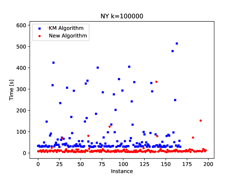
Figure 4: Results obtained from the $200$ instances (if solved) defined on NY networks with $k=10^{5}$.

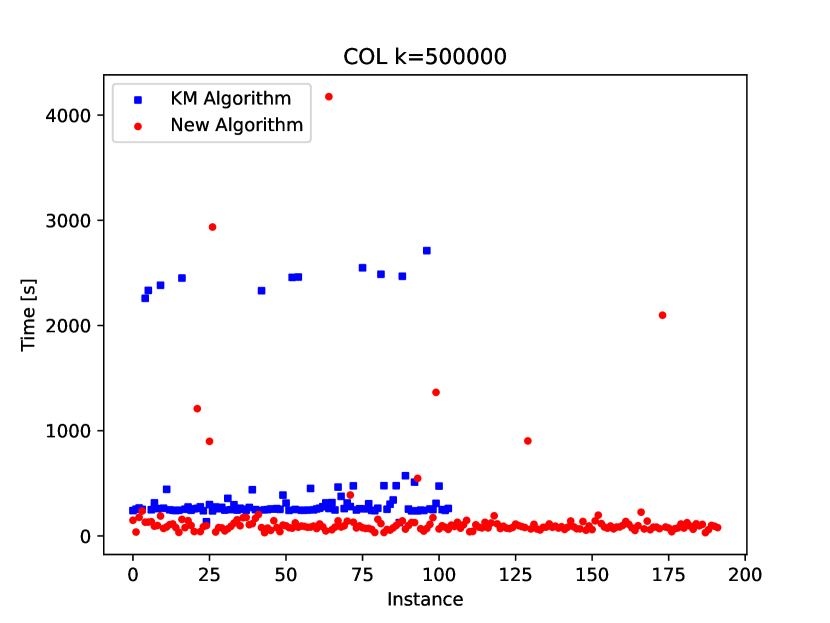
Figure 5: Results obtained from the $200$ instances (if solved) defined on COL networks with $k=5\times 10^{5}$.

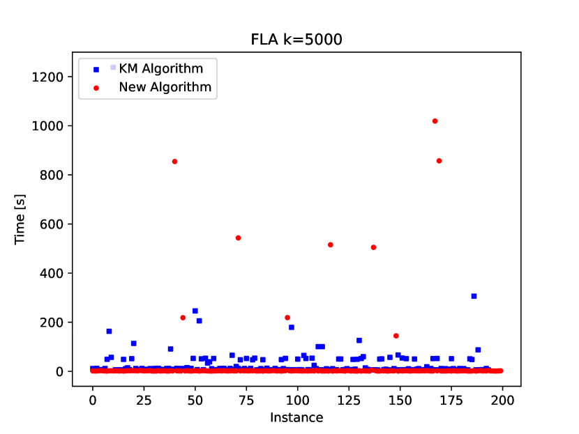
Figure 6: Results obtained from the $200$ instances defined on FLA networks with $k=5000$.

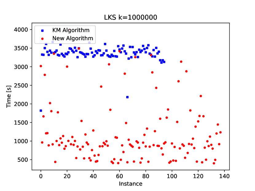
Figure 7: Results obtained from the $200$ instances (if solved) defined on LKS networks with $k=10^{6}$.

Table 5: Results obtained from the $k$-SSP instances defined on road networks. If Iterations ✗ is a small number, the non-existence of a relevant second shortest path could be proven fast (cf. Section 4.2).

$k$	KM			Algorithm 1						SPEEDUP
	Solved	Trees	Time	Solved	$\text{BDA}_{2\text{SSP}}$	$\text{BDA}_{2\text{SSP}}$ ✗	Iterations ✓	Iterations ✗	Time
NY
10	200	1	0.05	200	15	4	186	130	0.10	0.52
100	200	4	0.15	200	188	51	140	98	0.12	1.28
1000	200	20	1.13	200	1935	523	112	88	0.23	4.98
5000	200	109	4.48	200	9760	2677	100	82	0.68	6.57
10000	197	220	8.98	200	19552	5363	96	79	1.18	7.61
50000	182	987	47.34	200	97824	26736	88	76	5.20	9.11
100000	168	1643	113.67	198	196277	53170	84	69	9.73	11.68
500000	125	4405	867.08	198	980103	266634	78	66	48.72	17.80
1000000	91	4116	1975.73	196	1959033	532676	77	61	90.82	21.75
BAY
10	200	2	0.07	200	14	3	215	168	0.10	0.71
100	200	6	0.20	200	189	50	182	144	0.12	1.67
1000	200	67	2.00	200	1961	520	145	134	0.30	6.70
5000	198	439	11.17	200	9868	2650	128	123	0.96	11.63
10000	190	847	23.18	200	19758	5303	122	119	1.70	13.60
50000	151	3598	170.32	199	98883	26579	111	113	7.97	21.37
100000	127	5710	438.19	199	197836	53240	107	113	16.77	26.13
500000	61	12297	2528.40	190	991928	263977	104	81	77.39	32.67
1000000	40	15572	4113.70	189	1983487	526322	101	79	138.60	29.68
COL
10	200	1	0.09	200	11	3	128	152	0.13	0.69
100	200	3	0.22	200	141	46	109	133	0.15	1.41
1000	200	11	1.81	200	1557	420	79	123	0.33	5.45
5000	198	38	9.61	200	8300	2506	70	120	1.10	8.76
10000	193	62	16.38	200	16930	4763	70	120	2.09	7.83
50000	156	98	138.73	198	86874	25251	73	112	11.11	12.49
100000	140	117	337.81	195	174875	48851	73	97	23.33	14.48
500000	104	115	1433.21	192	883570	234159	69	92	106.66	13.44
1000000	92	124	2396.19	188	1802480	459770	72	86	202.93	11.81
CAL
10	200	1	0.46	200	11	4	258	281	0.58	0.79
100	200	2	0.83	200	141	45	257	203	0.63	1.32
1000	200	5	4.20	200	1680	374	223	193	1.24	3.38
5000	197	16	19.48	200	9122	2374	214	186	4.43	4.39
10000	192	25	42.71	200	18463	4760	204	178	8.56	4.99
50000	166	61	317.06	197	95921	24492	185	145	47.17	6.72
100000	152	81	654.53	198	192603	49266	179	149	92.33	7.09
500000	93	208	2942.28	195	964115	246741	165	129	454.34	6.48
1000000	82	325	4287.38	178	1946894	500079	172	124	927.41	4.62
FLA
10	200	1	0.21	200	10	4	176	162	0.32	0.66
100	200	2	0.52	200	132	41	147	194	0.37	1.41
1000	200	5	3.46	200	1468	417	105	198	0.80	4.34
5000	194	14	17.44	200	7853	2448	78	181	2.63	6.64
10000	188	22	30.58	200	15763	4858	72	179	5.17	5.91
50000	168	51	184.12	193	80003	23883	67	113	24.91	7.39
100000	147	43	505.38	192	161864	47771	72	107	42.20	11.98
500000	114	38	2190.95	187	821343	229620	85	98	220.34	9.94
1000000	92	51	3413.61	174	1699749	464313	111	88	512.08	6.67
LKS
10	200	1	0.53	200	10	3	172	242	0.82	0.64
100	200	1	0.99	200	114	45	175	176	0.87	1.14
1000	200	2	5.25	200	1242	344	139	138	1.52	3.46
5000	198	3	26.58	200	6638	2102	130	167	4.71	5.65
10000	194	4	52.56	200	13596	4470	123	176	9.25	5.68
50000	182	4	317.58	199	69638	23313	102	144	49.39	6.43
100000	172	4	653.23	199	141236	47241	97	144	96.96	6.74
500000	122	5	2883.55	171	735793	231196	95	134	657.57	4.39
1000000	95	7	4692.76	138	1595516	437025	97	131	1465.32	3.20
CTR
10	200	1	4.39	200	9	4	200	285	5.42	0.81
100	200	1	8.63	200	105	43	194	204	5.70	1.51
1000	200	1	45.66	200	1086	288	159	153	9.42	4.85
5000	199	1	213.61	199	5585	1943	142	147	32.08	6.66
10000	198	1	431.95	199	11366	4135	129	150	69.49	6.22
50000	168	2	2135.44	199	59046	22443	107	162	433.13	4.93
100000	154	2	4034.49	198	119179	43441	109	151	916.97	4.40

References

- Roditty and Zwick [2012] Liam Roditty and Uri Zwick. Replacement Paths and k Simple Shortest Paths in Unweighted Directed Graphs. ACM Trans. Algorithms, 8(4), October 2012. ISSN 1549-6325. doi:10.1145/2344422.2344423.
- Clarke et al. [1963] S. Clarke, A. Krikorian, and J. Rausen. Computing the n best loopless paths in a network. Journal of the Society for Industrial and Applied Mathematics, 11(4):1096–1102, 1963. ISSN 03684245. URL http://www.jstor.org/stable/2946497.
- Eppstein [2016] David Eppstein. k-Best Enumeration, pages 1003–1006. Springer New York, New York, NY, 2016. ISBN 978-1-4939-2864-4. doi:10.1007/978-1-4939-2864-4_733.
- Ehrgott [2005] M. Ehrgott. Multicriteria Optimization. Springer-Verlag, 2005. doi:10.1007/3-540-27659-9.
- Lawler [1972] E. L. Lawler. A procedure for computing the k best solutions to discrete optimization problems and its application to the shortest path problem. Management Science, 18(7):401–405, 1972. ISSN 00251909, 15265501. URL http://www.jstor.org/stable/2629357.
- Yen [1972] J. Y. Yen. Finding the Lengths of All Shortest paths in N-Node Nonnegative-Distance Complete Networks Using N3 Additions and N3 Comparisons. Journal of the ACM (JACM), 19(3):423–424, 1972.
- Dijkstra [1959] E. W. Dijkstra. A note on two problems in connexion with graphs. Numerische Mathematik 1, 1(1):269–271, December 1959. doi:10.1007/bf01386390.
- Fredman and Tarjan [1987] Michael L. Fredman and Robert Endre Tarjan. Fibonacci heaps and their uses in improved network optimization algorithms. Journal of the ACM, 34(3):596–615, July 1987. doi:10.1145/28869.28874.
- Martins and Pascoal [2003] E. Q. V. Martins and M. M. B. Pascoal. A new implementation of Yen’s ranking loopless paths algorithm. Quarterly Journal of the Belgian, French and Italian Operations Research Societies, 1(2), June 2003. doi:10.1007/s10288-002-0010-2.
- Kurz and Mutzel [2016] Denis Kurz and Petra Mutzel. A Sidetrack-Based Algorithm for Finding the k Shortest Simple Paths in a Directed Graph, 2016.
- Eppstein [1998] David Eppstein. Finding the k Shortest Paths. SIAM Journal on Computing, 28(2):652–673, 1 1998. doi:10.1137/s0097539795290477.
- Feng [2014a] Gang Feng. Finding k shortest simple paths in directed graphs: A node classification algorithm. Networks, 64(1):6–17, 3 2014a. doi:10.1002/net.21552.
- Gotthilf and Lewenstein [2009] Zvi Gotthilf and Moshe Lewenstein. Improved algorithms for the k simple shortest paths and the replacement paths problems. Information Processing Letters, 109(7):352–355, March 2009. doi:10.1016/j.ipl.2008.12.015.
- Pettie [2004] Seth Pettie. A new approach to all-pairs shortest paths on real-weighted graphs. Theoretical Computer Science, 312(1):47–74, 2004. ISSN 0304-3975. doi:10.1016/S0304-3975(03)00402-X. Automata, Languages and Programming.
- Orlin and Végh [2022] James B. Orlin and László Végh. Directed Shortest Paths via Approximate Cost Balancing. J. ACM, 70(1), 12 2022. ISSN 0004-5411. doi:10.1145/3565019.
- Sedeño-Noda [2016] Antonio Sedeño-Noda. Ranking One Million Simple Paths in Road Networks. Asia-Pacific Journal of Operational Research, 33(05):1650042, October 2016. doi:10.1142/s0217595916500421.
- Feng [2014b] Gang Feng. Improving Space Efficiency With Path Length Prediction for Finding Shortest Simple Paths. IEEE Transactions on Computers, 63(10):2459–2472, 2014b. doi:10.1109/TC.2013.136.
- Martins et al. [1999] Ernesto de Queirós Vieira Martins, Marta Margarida Braz Pascoal, and José Luis Santos. Deviation Algorithms For Ranking Shortest Paths. International Journal of Foundations of Computer Science, 10(03):247–261, September 1999. doi:10.1142/s0129054199000186.
- Roditty and Zwick [2005] Liam Roditty and Uri Zwick. Replacement Paths and k Simple Shortest Paths in Unweighted Directed Graphs. In Luís Caires, Giuseppe F. Italiano, Luís Monteiro, Catuscia Palamidessi, and Moti Yung, editors, Automata, Languages and Programming, pages 249–260, Berlin, Heidelberg, 2005. Springer Berlin Heidelberg. ISBN 978-3-540-31691-6.
- Sedeño Noda and Colebrook [2019] Antonio Sedeño Noda and Marcos Colebrook. A Biobjective Dijkstra Algorithm. European Journal of Operational Research, 276(1):106–118, July 2019. doi:10.1016/j.ejor.2019.01.007.
- Maristany de las Casas et al. [2021a] Pedro Maristany de las Casas, Ralf Borndörfer, Luitgard Kraus, and Antonio Sedeño-Noda. An FPTAS for Dynamic Multiobjective Shortest Path Problems. Algorithms, 14(2), 2021a. ISSN 1999-4893. doi:10.3390/a14020043.
- Maristany de las Casas et al. [2021b] Pedro Maristany de las Casas, Antonio Sedeño-Noda, and Ralf Borndörfer. An Improved Multiobjective Shortest Path Algorithm. Computers and Operations Research, 135:105424, 2021b. ISSN 0305-0548. doi:10.1016/j.cor.2021.105424.
- Ahmadi et al. [2021] S. Ahmadi, G. Tack, D. Harabor, and P. Kilby. Bi-Objective Search with Bi-Directional A*. In Petra Mutzel, Rasmus Pagh, and Grzegorz Herman, editors, 29th Annual European Symposium on Algorithms (ESA 2021), volume 204 of Leibniz International Proceedings in Informatics (LIPIcs), pages 3:1–3:15, Dagstuhl, Germany, 2021. Schloss Dagstuhl – Leibniz-Zentrum für Informatik. ISBN 978-3-95977-204-4. doi:10.4230/LIPIcs.ESA.2021.3.
- Maristany de las Casas et al. [2023] Pedro Maristany de las Casas, Luitgard Kraus, Antonio Sedeño-Noda, and Ralf Borndörfer. Targeted multiobjective Dijkstra algorithm. Networks, n/a(n/a), 2023. doi:10.1002/net.22174.
- Hansen [1980] Pierre Hansen. Bicriterion Path Problems. In Günter Fandel and Tomas Gal, editors, Multiple Criteria Decision Making Theory and Application, pages 109–127, Berlin, Heidelberg, 1980. Springer Berlin Heidelberg. ISBN 978-3-642-48782-8.
- Jochen Gorski and Sudhoff [2023] Kathrin Klamroth Jochen Gorski and Julia Sudhoff. Biobjective optimization problems on matroids with binary costs. Optimization, 72(7):1931–1960, 2023. doi:10.1080/02331934.2022.2044479.
- Bökler [2018] F. K. Bökler. Output-sensitive complexity of multiobjective combinatorial optimization with an application to the multiobjective shortest path problem. PhD thesis, Technische Universität Dortmund, 2018.
- Williams and Williams [2018] Virginia Vassilevska Williams and R. Ryan Williams. Subcubic Equivalences Between Path, Matrix, and Triangle Problems. Journal of the ACM, 65(5):1–38, August 2018. doi:10.1145/3186893.
- Demetrescu et al. [2009] C. Demetrescu, A. Goldberg, and D. Johnson. 9th DIMACS Implementation Challenge - Shortest Paths. http://www.diag.uniroma1.it//~challenge9/, 2009. Accessed: 2021-12-15.
- Maristany de las Casas [2023] Pedro Maristany de las Casas. maristanyPedro/kshortestpaths: Initial Release – Preprint Citation, September 2023. doi: 10.5281/zenodo.8324671.