Decoupled Training:
Return of Frustratingly Easy Multi-Domain Learning

Abstract

Multi-domain learning (MDL) aims to train a model with minimal average risk across multiple overlapping but non-identical domains. To tackle the challenges of dataset bias and domain domination, numerous MDL approaches have been proposed from the perspectives of seeking commonalities by aligning distributions to reduce domain gap or reserving differences by implementing domain-specific towers, gates, and even experts. MDL models are becoming more and more complex with sophisticated network architectures or loss functions, introducing extra parameters and enlarging computation costs. In this paper, we propose a frustratingly easy and hyperparameter-free multi-domain learning method named Decoupled Training (D-Train). D-Train is a tri-phase general-to-specific training strategy that first pre-trains on all domains to warm up a root model, then post-trains on each domain by splitting into multi-heads, and finally fine-tunes the heads by fixing the backbone, enabling decouple training to achieve domain independence. Despite its extraordinary simplicity and efficiency, D-Train performs remarkably well in extensive evaluations of various datasets from standard benchmarks to applications of satellite imagery and recommender system.

Introduction

The success of deep learning models across a wide range of fields often relies on the fundamental assumption that the data points are independent and identically distributed (i.i.d.). However, in real-world scenarios, training and test data are usually collected from different regions, devices, or platforms, consisting of multiple overlapping but non-identical domains. For example, a popular satellite dataset named Functional Map of the World (FMoW)  (Christie et al. 2018), which aims to predict the functional purpose of buildings and land use on this planet, contains large-scale satellite images from various regions with different appearances and styles. In this case, jointly training a single model obscures domain distinctions, while separately training multiple models by domains reduces training data in each model (Joshi et al. 2012). This dilemma motivated the research on multi-domain learning (Joshi et al. 2012; Liu, Qiu, and Huang 2017; Ma et al. 2018; Alice et al. 2019; Tang et al. 2020).

To figure out the challenges of multi-domain learning, we first delved into these two standard benchmark datasets. By analyzing the examples of these datasets, it is obvious that dataset bias across domains is one of the biggest obstacles to multi-domain learning. As shown in Figure 1(a), reviews from different domains have different keywords and styles. Further, Figure 1(b) reveals that images of Office-Home are from four significantly different domains: Art, Clipart, Product and Real-World, with various appearances and backgrounds. To tackle the dataset bias problem, numerous approaches have been proposed and they can be briefly grouped into two categories: 1) Seeking Commonalities. Some classical solutions (Liu, Qiu, and Huang 2017; Alice et al. 2019) adopting the insightful idea of domain adversarial training have been proposed to extract domain-invariant representations across multiple domains. 2) Reserving Differences. These approaches  (Ma et al. 2018; Tang et al. 2020) adopt multi-branch network architectures with domain-specific towers, gates, and even experts, implementing domain-specific parameters to avoid domain conflict caused by dataset bias across domains. As shown in Figure 2, these methods are becoming more and more complex with sophisticated network architectures or loss functions.

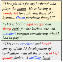
(a) Review Examples of MDL

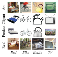
(b) Visual Examples of MDL

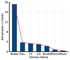
(c) #Samples in Amazon

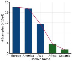
(d) #Samples in FMoW

Figure 1: (a)-(b): Review examples from a recommender system benchmark named Amazon with various styles and keywords, as well as visual examples from a computer vision dataset named Office-Home with various appearances and backgrounds, reveal the main challenge of dataset bias. (c)-(d): The distribution of sample number across domains is naturally imbalanced or even long-tailed, indicating another major challenge of domain domination.

Further, different from multi-task learning which focuses on tackling different tasks within a single domain, multi-domain learning shares the same label space across multiple domains with different marginal distributions. We thus calculated the distribution of sample number across domains on several benchmark datasets and the results are shown in Figure 1. In practice, the distributions of sample number across domains are usually twisted, imbalanced, or even long-tailed, causing another main challenge of multi-domain learning: domain domination. In this case, some tailed domains may have much fewer examples and it would be difficult to train satisfied models on them. Without proper network designs or loss functions, the model will be easily dominated by the head domains with much more examples and shift away from the tailed ones with few examples.

Realizing the main challenges of dataset bias and domain domination in multi-domain learning, we aim at proposing a general, effective, and efficient method to tackle these obstacles all at once. We first rethought the development of multi-domain learning and found that the approaches in this field are becoming more and more sophisticated, consisting of multifarious network architectures or complex loss functions with many trade-off hyperparameters. By assigning different parameters across domains, these designs may be beneficial in some cases but they will absolutely include more parameters and enlarge computation cost, as well as introduce much more hyperparameters. For example, the latest state-of-the-art method named PLE has to tune the numbers of domain-specific experts and domain-agnostic experts in each layer and design the network structures of each expert, each tower, and each gate network.

Motivated by the famous quote of Albert Einstein, “everything should be made as simple as possible, but no simpler”, we proposed a frustratingly easy multi-domain learning method named Decoupled Training (D-Train). D-Train is a training strategy based on the original frustratingly easy but most general shared-bottom architecture. D-Train is a tri-phase general-to-specific training strategy that first pre-trains on all domains to warm up a root model, then post-trains on each domain by splitting into multi-heads, and finally fine-tunes the heads by fixing the backbone, enabling decouple training to achieve domain independence. Despite its extraordinary simplicity and efficiency, D-Train performs remarkably well in extensive evaluations of various datasets from standard benchmarks to applications of satellite imagery and recommender system. In summary, this paper has the following contributions:

• We explicitly uncover the main challenges of dataset bias and domain domination in MDL, especially the latter since it is usually ignored in most existing works.

• We propose a frustratingly easy and hyperparameter-free MDL method named Decoupled Training by applying a tri-phase general-to-specific training strategy.

• We conduct extensive experiments from standard benchmarks to real-world applications and verify that D-Train performs remarkably well.

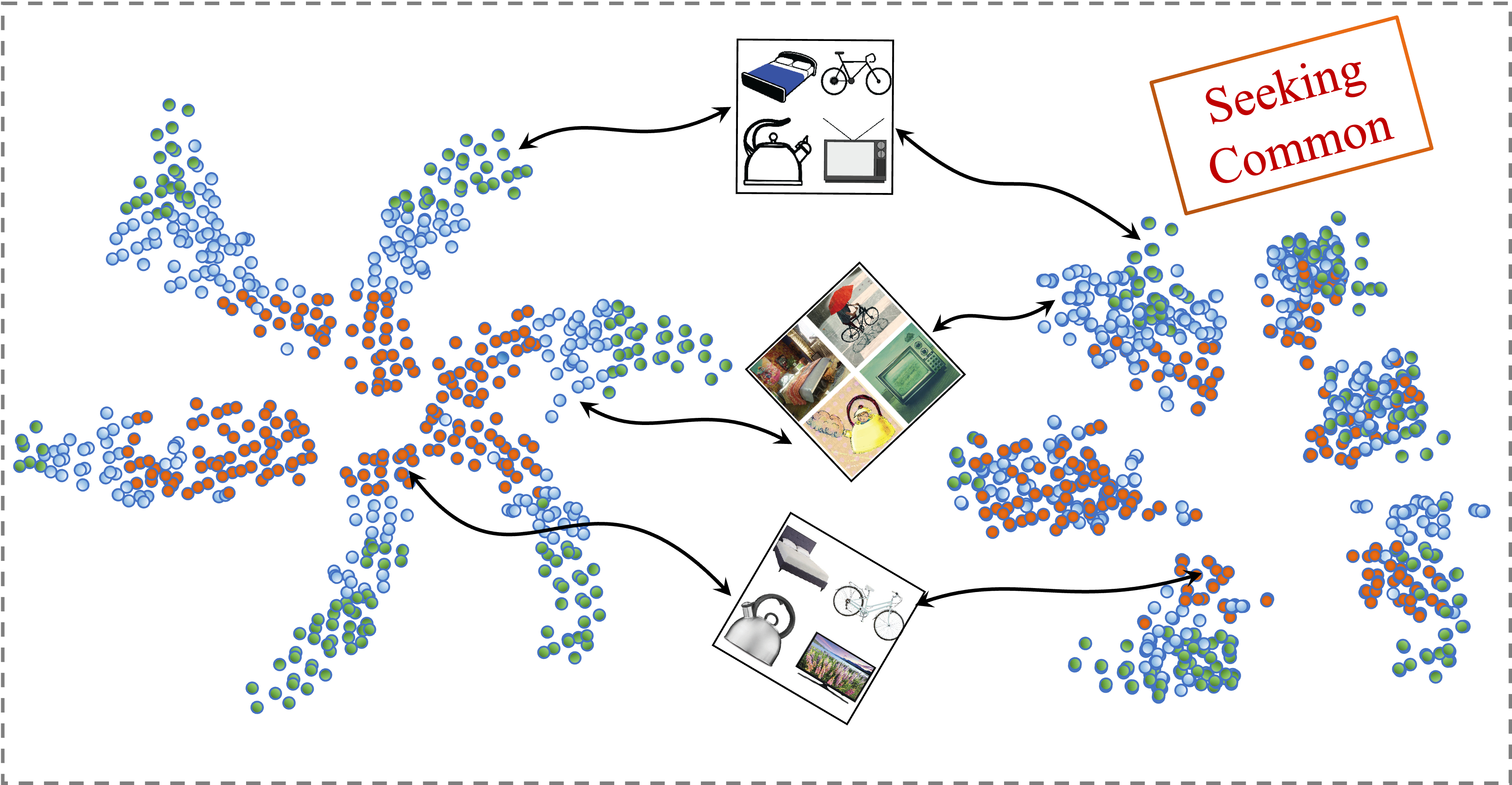
(a) Seeking Commonalities

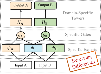
(b) Reserving Differences

Figure 2: (a): Seeking Commonalities by aligning distributions across domains to reduce domain gap. (b): Reserving Differences by implementing domain-specific towers, gates, and even experts.

Related Work

Seeking Commonalities

To tackle the dataset bias problem in multi-domain learning, various approaches (Liu, Qiu, and Huang 2017; Alice et al. 2019) have been proposed from the perspective of domain alignment, by adopting the insightful idea of domain adversarial training to extract domain-invariant representations across domains. To smooth the presentation of domain alignment in MDL, we will first give a brief review of domain adaptation. There are mainly two categories of domain adaptation formulas: covariate shift (Quionero-Candela et al. 2009; Pan and Yang 2010; Long et al. 2015; Ganin and Lempitsky 2015) and label shift (Lipton, Wang, and Smola 2018; Azizzadenesheli et al. 2019; Alexandari, Kundaje, and Shrikumar 2020), while we focus on the former in this paper since it is more relevant with the topic of MDL. Recent deep domain adaptation methods tackle domain shifts from the perspectives of either moment matching or adversarial training, in which the former aligns feature distributions by minimizing the distribution discrepancy across domains (Long et al. 2015; Tzeng et al. 2014; Long et al. 2017). Further, domain adversarial neural network (DANN) (Ganin et al. 2016) becomes the mainstream method in domain adaptation. It introduces a domain discriminator to distinguish the source features from the target ones, while the feature extractor is designed to confuse the domain discriminator. In this way, the domain discriminator and feature extractor are competing in a two-player minimax game. Its natural extension to MDL is DANN-MDL. Later, CDAN (Long et al. 2018) further tailors the discriminative information conveyed in the classifier predictions into the input of the domain discriminator, whose natural extension to MDL is CDAN-MDL. Following the main idea of the minimax game, several variants of adversarial training methods (Pei et al. 2018; Tzeng et al. 2017; Saito et al. 2018; Zhang et al. 2019) were proposed. MulANN (Alice et al. 2019) tailors the insight of domain adversarial training into the MDL problem by introducing a domain discriminator into the shared model with a single head. In contrast, ASP-MTL (Liu, Qiu, and Huang 2017) includes a shared-private model and a domain discriminator.

Reserving Differences

Another series of methods (Ma et al. 2018; Tang et al. 2020; Sheng et al. 2021) for multi-domain learning adopt multi-branch network architectures and develop domain-specific parameters (Dredze, Kulesza, and Crammer 2010) to avoid domain conflict caused by dataset bias across domains. Among them, Shared Bottom (SB) (Ruder 2017) is the frustratingly easy but effective one. Further, MoE (Jacobs et al. 1991) and its extension of MMoE (Ma et al. 2018) adopt the insightful idea of the mixture of experts to learn different mixture patterns of experts assembling, respectively. PLE (Tang et al. 2020) explicitly separates domain-shared and domain-specific experts to alleviate harmful parameter interference across domains. Note that, PLE further applies progressive separation routing with several deeper layers but we only adopt one layer for a fair comparison with other baselines. Other MDL methods focus on maintaining shared and domain-specific parameters by confidence-weighted combination (Dredze, Kulesza, and Crammer 2010), domain-guided dropout (Xiao et al. 2016), or prior knowledge about domain semantic relationships (Yang and Hospedales 2015). Meanwhile, various task-specific MDL approaches have been proposed for computer vision (Rebuffi, Bilen, and Vedaldi 2018; Mancini et al. 2020; Nam and Han 2016; Rebuffi, Bilen, and Vedaldi 2017; Li and Vasconcelos 2019; Fourure et al. 2017), natural language processing (Wu and Guo 2020; Williams 2013; Pham, Crego, and Yvon 2021) and recommender system (Hao et al. 2021; Chen et al. 2020; Du et al. 2019; Gu et al. 2021; Li et al. 2021b, a; Salah, Tran, and Lauw 2021). The comparison between these MDL methods are summarized in Figure 2.

Approach

This paper aims at proposing a simple, effective, and frustratingly easy method for multi-domain learning (MDL). Given data points from multiple domains $\{\mathcal{D}_{1},\mathcal{D}_{2},...,\mathcal{D}_{T}\}$, $T$ is the domain number. Denote $\mathcal{D}_{t}=\{(\mathbf{x}_{i},\mathbf{y}_{i})\}_{i=1}^{n_{t}}$ the data from domain $t$, where $\mathbf{x}_{i}$ is an example, $\mathbf{y}_{i}$ is the associated label and $n_{t}$ is the sample number of domain $t$. Denote the shared backbone $\psi$ and the domain-specific heads $\{{h}_{1},{h}_{2},...,{h}_{T}\}$ respectively. The goal of MDL is to improve the performance of each domain $\mathcal{D}_{t}$.

As mentioned above, the proposed Decoupled Training (D-Train) is a frustratingly easy multi-domain learning method based on the original shared-bottom architecture. D-Train takes a general-to-specific training strategy. It first pre-trains on all domains to warm up a root model. Then, it post-trains on each domain by splitting into multi-heads. Finally, it fine-tunes the heads by fixing the backbone, enabling decouple training to achieve domain independence.

(a) Training details of each phase

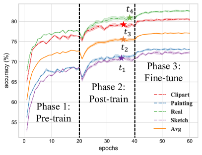
(b) Training curves of each phase

Figure 3: (a): Explanations of different phases of D-Train. $\psi$ denotes the feature extractor; $h$ denotes the shared head in the pre-training phase; $\{{h}_{1},{h}_{2},...,{h}_{T}\}$ denote the domain-specific heads at the next two phases. During the fine-tuning phase, the parameters of the feature extractor are fixed. (b): The training curves of each phase of D-Train on various domains: Clipart, Painting, Real and Sketch as shown in dotted lines, while the average accuracy over domains is shown in solid line.

Pre-train: warm up a root model

The power of deep learning models is unleashed by large-scale datasets. However, as mentioned in Section Introduction, the distributions of sample numbers across domains are usually twisted, imbalanced, or even long-tailed in real-world applications. In this case, some tailed domains may only have limited samples and it would be difficult to train satisfied models on them. To alleviate this problem, D-Train first pre-trains a single model on samples from all domains to warm up a root model for all domains, especially for the tailed domain with limited samples. The optimization function of the pre-train phase in multiple domains can be formalized as

$${\psi}_{0},{h}_{0}=\mathop{\arg\min}\limits_{\psi,h}{\frac{1}{T}\sum_{t=1}^{T}}\frac{1}{n_{t}}\sum_{i=1}^{n_{t}}\mathcal{L}\left[(h\circ\psi)(\mathbf{x}_{i}^{t}),\mathbf{y}_{i}^{t}\right],$$ (1)

where $h$ and $\psi$ are the shared head and backbone at the pre-training phase. After the training process converges, $\psi_{0}$ and ${h}_{0}$ will be good initializations for the next phase, as shown in Figure 3(a). To verify it, we take DomainNet as an example and show the training curves of the proposed method in Figure 3(b). Note that, the experiments are repeated $5$ times to show both mean and standard deviation.

Post-train: split into multi-heads

As mentioned before, jointly training a single model obscures domain distinctions, leading to domain conflict caused by the specificity of different domains. To reflect the domain specificity and achieve satisfactory performance for each domain, we adopt the shared-bottom architecture that has a shared feature extractor $\psi$ and various domain-specific heads $\{{h}_{1},{h}_{2},...,{h}_{T}\}$ to tackle the challenge of dataset bias across domains. With this design, the parameters of the feature extractor will be updated simultaneously by gradients of samples from all domains, but the parameters of domain-specific heads are trained on each domain. The optimization function of the post-training phase over all domains can be formalized as

$$\widetilde{\psi},\{\widetilde{h}_{1},\widetilde{h}_{2},...,\widetilde{h}_{T}\}=\mathop{\arg\min}\limits_{\psi,\{{h}_{1},{h}_{2},...,{h}_{T}\}}{\frac{1}{T}\sum_{t=1}^{T}}L_{t}$$ (2)

$$L_{t}=\frac{1}{n_{t}}\sum_{i=1}^{n_{t}}\mathcal{L}\left[(h_{t}\circ\psi)(\mathbf{x}_{i}^{t}),\mathbf{y}_{i}^{t}\right]$$ (3)

where the domain-agnostic feature extractor $\psi$ is initialized as ${\psi}_{0}$ while each domain-specific head $h_{t}$ of domain $t$ is initialized as ${h}_{0}$. After the training process converges, $\psi$ and ${h}$ will reach strong points of $\widetilde{\psi}$ and $\widetilde{h}$ as shown in Figure 3(b). Since the shared-bottom architecture contains both domain-agnostic and domain-specific parameters, the training across domains maintains a lukewarm relationship. In this way, the challenge of dataset bias across domains and domain domination can be somewhat alleviated. The training curves as shown in Figure 3(b) also witness a sharp improvement via splitting into multi-heads across domains. Note that, at the beginning of the post-train phase, the test accuracy of each domain drops first owing to the training mode switches from fitting all domains to each specific domain.

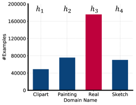
(a) Domain Domination

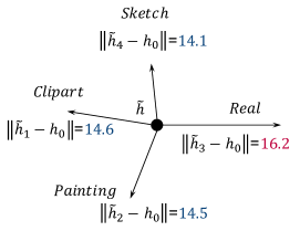
(b) After Post-train

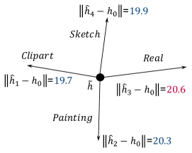
(c) After Fine-tune

Figure 4: Analysis on the domain domination challenge where ${h}_{0}$ is the domain-agnostic head at the pre-training phase. $\|\cdot\|$ denotes the Euclidean norm of the parameter update between different phases.

Table 1: Accuracy (%) on Office-Home for multi-domain learning (ResNet-50).

Method	Art	Clipart	Product	Real-World	Avg. Acc.	Worst Acc.
#Samples	2427	4365	4439	4357	-	-
Separatly Train	76.8	77.2	92.9	87.1	83.5	76.8
Jointly Train	73.5	73.3	91.4	86.7	81.2	73.3
MulANN (Alice et al. 2019)	77.8	80.0	92.5	87.3	84.4	77.8
DANN-MDL (Ganin et al. 2016)	75.9	77.2	92.2	87.2	83.1	75.9
ASP-MDL (Liu, Qiu, and Huang 2017)	78.8	79.3	93.2	87.5	84.7	78.8
CDAN-MDL (Long et al. 2018)	78.6	79.0	93.6	89.1	85.1	78.6
Shared Bottom (Ruder 2017)	76.5	80.2	93.8	88.8	84.8	76.5
MoE (Jacobs et al. 1991)	76.8	77.1	92.3	87.4	83.4	76.8
MMoE (Ma et al. 2018)	78.8	79.6	93.4	88.9	85.2	78.8
PLE (Tang et al. 2020)	78.0	79.8	93.6	88.5	85.0	78.0
D-Train (ours)	80.0	80.3	94.1	89.5	86.0	80.0

Fine-tune: decouple-train for domain independence

Regarding the benefits of domain-specific parameters across domains, a natural question arises: Can the shared-bottom architecture fully solve the problem of domain domination? To answer this question, we adopt the Euclidean norm to calculate the parameter update between the domain-specific heads $\{{h}_{1},{h}_{2},...,{h}_{T}\}$ and the domain-agnostic head ${h}_{0}$ at the pre-training phase on DomainNet. As shown in Figure 4(a), the domain of Real has much more examples than other domains, and is believed to dominate the training process. However, as shown in Figure 4(b), the parameter update after the post-train phase reveal that the training process is still dominated by the head domain which still has the largest value of the parameter update. Hence, though the challenge of dataset bias across domains can be alleviated by introducing domain-specific heads in the shared-bottom architecture, the domain domination problem still exists after the post-train phase. This is reasonable since the domain-shared parameters of the backbone will be dominated by the head domains. To this end, we propose a decoupling training strategy by fully fixing the parameters of the feature extractor to achieve domain independence. Formally,

$$\widehat{h}_{t}=\mathop{\arg\min}\limits_{h_{t}}\frac{1}{n_{t}}\sum_{i=1}^{n_{t}}\mathcal{L}\big{[}(h_{t}\circ\widetilde{\psi})(\mathbf{x}_{i}^{t}),\mathbf{y}_{i}^{t}\big{]},\quad t=1,2,...,T.$$ (4)

In this way, the parameters of the domain-specific heads will be learned by samples from each domain as shown in Figure 3(a). With this kind of domain-independent training, the head domains will no longer dominate the training of the tailed domains at this phase. Further, the parameter update between phases becomes more balanced across domains as shown in Figure 4(c). Meanwhile, the training curves as shown in Figure 3(b) reveal that fine-tuning across domains can further improve the performance.

Why does D-Train work?

As mentioned before, dataset bias and domain domination are the main challenges of multi-domain learning. All of the existing works, including the methods from the perspectives of both seeking commonalities or reserving differences, have to face the challenge of caring for this and losing that. With the shared parameters across domains, these methods will influence each other. When the problem of domain domination or the domain conflict caused by dataset bias cannot be ignored, the MDL model will struggle in finding an optimal solution for all domains. Actually, as shown in the training process of DomainNet in Figure 3(b), different domains achieve the optimal performance at different time stamps after the post-training phase. However, the goal of multi-domain learning is to use one model to serve all domains, and thus we cannot use these models simultaneously. On the contrary, with the proposed decoupling training strategy, different domains in D-Train will train independently at the fine-tuning phase and reach an optimal solution for each domain.

Experiments

In this section, we compared the proposed D-Train method with three categories of baselines: Single Branch, Domain Alignment, and Multiple Branch.

Table 2: Accuracy (%) on DomainNet for multi-domain learning (ResNet-101).

Method	Clipart	Painting	Real	Sketch	Avg. Acc.	Worst Acc.
#Samples	49k	76k	175k	70k	-	-
Separatly Train	78.2	71.6	83.8	70.6	76.1	70.6
Jointly Train	77.4	68.0	77.9	68.5	73.0	68.0
MulANN (Alice et al. 2019)	79.5	71.7	81.7	69.9	75.7	69.9
DANN-MDL (Ganin et al. 2016)	79.8	71.4	81.4	70.3	75.7	70.3
ASP-MDL (Liu, Qiu, and Huang 2017)	80.1	72.1	81.2	70.9	76.1	70.9
CDAN-MDL (Long et al. 2018)	80.2	72.2	81.3	71.0	76.2	71.0
Shared Bottom (Ruder 2017)	79.9	72.1	81.9	69.7	75.9	69.7
MoE (Jacobs et al. 1991)	79.1	70.2	79.8	69.4	74.6	69.4
MMoE (Ma et al. 2018)	79.6	72.2	82.0	69.8	75.9	69.8
PLE (Tang et al. 2020)	80.0	72.2	82.1	70.0	76.1	70.0
D-Train (w/o Fine-tune)	79.9	71.3	81.3	70.9	75.9	70.9
D-Train (w/o Post-train)	79.8	72.9	81.7	72.1	76.6	72.1
D-Train (w/o Pre-train)	80.9	72.9	82.7	71.5	77.0	71.5
D-Train (ours)	81.5	72.8	82.7	72.2	77.3	72.2

Standard Benckmarks

In this section, we adopt two standard benchmarks in the field of domain adaptation with various dataset scales, in which Office-Home is in a low-data regime and DomainNet is a large-scale one. D-Train and all baselines in this section are implemented in a popular open-sourced library  which has implemented a high-quality code base for many domain adaptation baselines.

Low-data Regime: Office-Home

Office-Home is a standard multi-domain learning dataset  (Venkateswara et al. 2017) with $65$ classes and $15,500$ images from four significantly different domains: Art, Clipart, Product, and Real-World. As shown in Figure 1(b), there exist challenges of dataset bias and domain domination in this dataset. Following existing works on this dataset, we adopt ResNet-50 as the backbone and randomly initialize fully connected layers as heads. We set the learning rate as $0.0003$ and batch size as $24$ in each domain for D-Train and all baselines.

As shown in Table 1, Separately Training is a strong baseline and even outperforms Jointly Training, since the latter obscures domain distinctions and cannot tackle the dataset bias across domains. Multi-Domain Learning methods from the perspective of domain alignment work much better by introducing a domain discriminator and exploiting the domain information. However, applying domain alignment is not an optimal solution in MDL since the domain gap can only be reduced but not removed. Finally, the proposed D-Train consistently improves on all domains, even the tailed domain of “Art”. D-Train achieves a new state-of-the-art result with an average accuracy of $86.0$.

Large-Scale Dataset: DomainNet

DomainNet (Peng et al. 2019) is a large-scale multi-domain learning and domain adaptation dataset with $345$ categories. We utilize $4$ domains with different appearances including Clipart, Painting, Real, and Sketch where each domain has about $40,000$ to $200,000$ images. As shown in Figure 4(a), the domain of ”Real” has much more examples than other domains, and is believed to dominate the training process. Following the code base in Transfer Learning Library, we adopt mini-batch SGD with the momentum of $0.9$ as an optimizer, and the initial learning rate is set as $0.01$ with an annealing strategy. We adopt ResNet-101 as the backbone since DomainNet is much larger and more difficult than the previous Office-Home dataset. Meanwhile, the batch size is set as $20$ in each domain here for D-Train and all baselines.

As shown in Table 2, the proposed D-Train outperforms all baselines, no matter measured by average accuracy or worst accuracy in all domains. Since the domain of “Real” has much more samples than other domains, it achieves competitive performance while separately training. However, other domains benefit from training via D-Train.

Applications of Satellite Imagery

In this section, we adopt a popular satellite dataset named Functional Map of the World (FMoW)  (Christie et al. 2018), which aims to predict the functional purpose of buildings and land use on this planet, contains large-scale satellite images with different appearances and styles from various regions: Africa, Americas, Asia, Europe, and Oceania. FMoW is a natural dataset for multi-domain learning. D-Train and all baselines in this section are implemented in a popular open-sourced library named WILDS  since it enables easy manipulation of this dataset. Each input $\mathbf{x}$ in FMoW is an RGB satellite image that is resized to $224\times 224$ pixels and the label $y$ is one of $62$ building or land use categories. For all experiments, we follow (Christie et al. 2018) and use a DenseNet-121 model (Huang et al. 2017) pretrained on ImageNet. We set the batch size to be $64$ on all domains. Following WILDS, we report the average accuracy and worst-region accuracy in all multi-domain learning methods.

Table 3: Accuracy (%) on FMoW for multi-domain learning (DenseNet-121).

Method	Asia	Europe	Africa	America	Oceania	Avg. Acc.	Worst Acc.
#Samples	115k	182k	37k	176k	15k	-	-
Separatly Train	59.4	56.9	72.9	59.4	65.1	58.7	56.9
Jointly Train	60.8	57.2	77.0	63.5	71.6	60.4	57.2
MulANN (Alice et al. 2019)	61.2	57.5	74.6	62.3	67.9	60.2	57.5
DANN-MDL (Ganin et al. 2016)	55.9	55.5	61.9	58.2	74.2	56.7	55.5
ASP-MDL (Liu, Qiu, and Huang 2017)	54.5	53.9	73.4	57.4	70.3	55.3	53.9
CDAN-MDL (Long et al. 2018)	57.0	56.8	68.0	59.7	70.3	57.7	56.8
Shared Bottom (Ruder 2017)	58.1	57.1	75.4	61.3	71.9	59.8	57.1
MoE (Jacobs et al. 1991)	55.9	54.0	63.2	59.0	70.6	56.3	54.0
MMoE (Ma et al. 2018)	60.7	55.7	65.6	62.4	64.8	58.7	55.7
PLE (Tang et al. 2020)	58.2	56.5	74.6	61.7	72.5	59.0	56.5
D-Train (ours)	62.3	58.3	77.0	62.7	68.3	61.0	58.3

As shown in Table 3, it’s not wise to train a separate model for each domain on FMoW, since the data on some domains is extremely scarce. Joint Train or Shared Bottom is also not optimal, because conflicts widely exist in some domains, such as the Europe domain and Africa domain which have very different appearances. Note that D-Train also outperforms all baselines in this difficult dataset.

Table 4: AUC (%) on Amazon Product Review for multi-domain learning.

Method	Books	Elec.	TV	CD	Kindle	Phone	Music	$\texttt{AUC}_{d}$	$\texttt{AUC}_{s}$
#Samples	19.2M	3.70M	3.28M	2.96M	2.25M	0.81M	0.38M	–	–
Separately Training	66.09	77.50	79.43	59.69	52.79	70.06	52.95	65.50	67.17
Jointly Training	69.01	78.87	85.06	64.24	59.15	69.89	49.71	67.99	70.43
MulANN (Alice et al. 2019)	68.95	78.90	84.56	64.79	58.64	70.43	52.13	68.34	70.40
DANN-MDL (Ganin et al. 2016)	68.64	80.33	86.08	66.32	58.59	72.47	54.21	69.52	70.74
CDAN-MDL (Long et al. 2018)	69.74	80.63	85.88	67.24	60.61	73.34	57.39	70.69	71.69
MoE (Jacobs et al. 1991)	73.51	85.88	89.66	74.94	63.45	79.63	66.08	76.16	76.04
Shared Bottom (Ruder 2017)	70.91	74.87	85.51	67.18	60.56	74.59	59.14	70.39	71.73
Shared Bottom + D-Train	71.35	74.76	85.52	67.61	60.20	73.53	61.61	70.65	71.99
MMoE (Ma et al. 2018)	73.67	86.15	89.23	75.50	62.43	81.91	63.69	76.01	76.13
MMoE + D-Train	74.50	86.09	88.60	77.13	66.46	82.13	69.01	77.70	77.05
PLE (Tang et al. 2020)	75.25	85.36	88.54	76.09	69.35	81.02	67.75	77.62	77.46
PLE + D-Train	74.70	86.70	89.53	77.40	69.26	82.47	69.91	78.57	77.56

Applications of Recommender System

In this section, we adopt a popular dataset named Amazon Product Review (Amazon) . We select $7$ typical subsets with various scales including Books (Books), Electronics (Elec.), Movies_and_TV (TV), CDs_and_Vinyl (CD), Kindle_Store (Kindle), Cell_Phones_and_Accessories (Phone), Digital_Music (Music). As shown in Tabel 4, different domains have various samples from $0.38M$ to $19.2M$. For each domain, diverse user behaviors are available, including more than $5$ reviews for each user-goods pair. The features used for experiments consist of goods_id and user_id. It is obvious that users in these domains have different preferences for various goods.

D-Train and all baselines in this section are implemented based on a popular open-sourced library named pytorch-fm . We use DNN as the CTR method and the embed_dim and mlp_dim are both set as $16$. The layer number of the expert and the tower are set as $2$ and $3$ respectively. We report AUC (Area Under the Curve) for each domain. Further, AUC_d and AUC_s are averaged over all domains and all samples respectively to intuitively compare D-Train with other baselines. For all models, we use Adam as the optimizer with exponential decay, in which the learning rate starts at $1e^{-3}$ with a decay rate of $1e^{-6}$. During training, the mini-batch size is set to $2048$. As shown in Table 4, D-Train yields larger improvements than a variety of MDL baselines on Amazon Product Review dataset.

Plug-in Unit

D-Train can be used as a general plug-in unit for existing MDL methods. We compare its performance with Shared Bottom, MMoE, and PLE, by only training the parameters of domain-specific heads while fixing the other parameters at the fine-tuning phase. As shown in Table 4, D-Train can further improve these competitive MDL methods on Amazon Product Review dataset, by tailoring D-Train into them.

Ablation Study

As shown in Table 2, we conduct an ablation study on DomainNet by removing each phase respectively. The reported results on four different domains reveal that only utilizing all of these phases works best. In particular, D-Train (w/o Fine-tune) works much worse than other ablation experiments, which reveals the importance of decoupling training for domain independence.

Conclusion

Multi-domain learning (MDL) is of great importance in both academia and industry. Numerous efforts have been paid for it but most of the works focus on a special application and a general approach is missing. In this paper, we explicitly uncover the main challenges of dataset bias and domain domination in multi-domain learning, especially the latter since it is usually ignored in most existing works. We further propose a frustratingly easy and hyperparameter-free multi-domain learning method named Decoupled Train (D-Train) with a tri-phase general-to-specific training strategy. Despite its extraordinary simplicity and efficiency, D-Train performs remarkably well in extensive evaluations of various datasets from standard benchmarks to applications of satellite imagery and recommender system.

Appendix A Experiment Details

Baselines

We use PyTorch as the deep learning framework and run all methods in Titan V. We compared the proposed D-Train method with three categories of baselines: Single Branch, Domain Alignment, and Multiple Branch. The implementation details of these baselines are summarized as follows:

• Separately Train is a strong baseline that separately trains on each domain when enough data is available as shown in Figure 5(f). Here, each domain is trained independently and samples from other domains will not influence the target domain. However, separately training multiple models by domains reduces training data in each model (Joshi et al. 2012).

• Jointly Train trains a single model with samples from all domains regardless of the domain information as shown in Figure 5(a). In this case, jointly training a single model obscures domain distinctions (Joshi et al. 2012) and it may bring the challenge of dataset bias.

• DANN-MDL (Ganin et al. 2016) is a direct extension of DANN in domain adaptation into multi-domain learning as shown in Figure 5(c). Here, we introduce a domain discriminator for the original MDL model to enable distribution alignment across domains.

• MulANN (Alice et al. 2019) introduces a domain discriminator into the shared model with a single head, as shown in Figure 5(b). Here, we remove the extra loss in the original paper on unlabeled data since all samples are labeled in our setting.

• ASP-MTL (Liu, Qiu, and Huang 2017) includes a domain-agnostic backbone, a domain-shared head, multiple domain-specific heads, and a domain discriminator, as shown in Figure 5(d). Similarly, the loss function specifically designed for natural language processing is removed.

• CDAN-MDL (Long et al. 2018) is a natural extension of CDAN to MDL as shown in Figure 5(e). Since we empirically found that ASP-MTL is much better than the other two variants of domain alignment methods, we also designed a share-private architecture for CDAN-MDL.

• Shared Bottom (SB) (Ruder 2017) is the frustratingly easy but effective MDL method, as shown in Figure 5(g). Here, a shared backbone is included to extract representations while multiple domain-specific heads are designed considering the specificity of each domain.

• MoE (Jacobs et al. 1991) utilizes the insightful idea of the mixture of experts that learns different mixtures patterns of experts assembling as shown in Figure 5(h). Here, the number of experts is selected from the set of $[3,4,5,6]$ according to the performance on the validation set.

• MMoE (Ma et al. 2018) extends MoE to the multi-gate version and explicitly learns to model task relationships from data by designing a task-specific gating network for each task, as shown in Figure 5(i). Similarly, the number of experts is selected from the set of $[3,4,5,6]$ according to the performance on the validation set of each experiment.

• PLE (Tang et al. 2020) explicitly separates domain-shared and domain-specific experts as shown in Figure 5(j). The PLE model in the original paper adopts a progressive routing mechanism to extract and separate deeper semantic knowledge gradually (Tang et al. 2020).

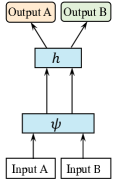
(a) Joint

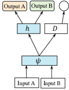
(b) MulANN

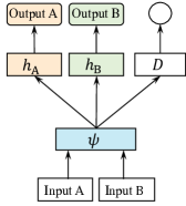
(c) DANN-MDL

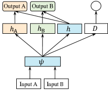
(d) ASP-MTL

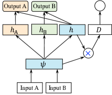
(e) CDAN-MDL

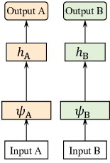
(f) Separate

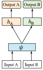
(g) SB

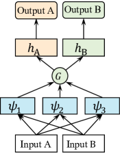
(h) MoE

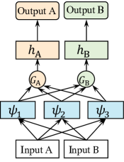
(i) MMoE

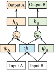
(j) PLE

Figure 5: Network architectures of various multi-domain learning methods in which methods at the top row tackle dataset shift from the perspective of domain alignment and methods at the bottom row adopt multi-branch architecture with domain-specific and domain-shared parameters. The used terminologies include feature extractor (backbone) $\psi$, classifier (head) $h$, domain discriminator $D$, and gate $G$. The blue items represent domain-shared modules while others are domain-specific modules.

Table 5: Comparisons among various MDL methods. Note that, $T$ is the domain number. $n_{\psi}$ and $n_{h}$ are parameter number of the backbone and head respectively. Usually, the inequality $n_{\psi}\gg n_{h}$ holds.

Method	#Parameters	Hyperparameters
Separately Train	$\mathcal{O}(T\cdot n_{\psi}+T\cdot n_{h})$	W/O
Jointly Train	$\mathcal{O}(n_{\psi}+n_{h})$	W/O
MulANN	$\mathcal{O}(n_{\psi}+n_{h}+n_{D})$	loss trade-off: $\lambda$; domain discriminator arch.
DANN-MDL	$\mathcal{O}(n_{\psi}+T\cdot n_{h}+n_{D})$	loss trade-off: $\lambda$; domain discriminator arch.
ASP-MTL	$\mathcal{O}(n_{\psi}+(T+1)\cdot n_{h}+n_{D})$	loss trade-off: $\lambda$; domain discriminator arch.
CDAN-MDL	$\mathcal{O}(n_{\psi}+(T+1)\cdot n_{h}+n_{D})$	loss trade-off: $\lambda$; domain discriminator arch.
Shared Bottom	$\mathcal{O}(n_{\psi}+T\cdot n_{h})$	W/O
MoE	$\mathcal{O}(E\cdot n_{\psi}+n_{G}+T\cdot n_{h})$	expert number (EN): $E$; gate network arch.
MMoE	$\mathcal{O}(E\cdot n_{\psi}+T\cdot(n_{h}+n_{G}))$	expert number (EN): $E$; gate network arch.
PLE	$\mathcal{O}((m_{s}+\sum_{i}^{T}m_{i})\cdot n_{\psi}+T\cdot n_{h})$	domain-share EN: $m_{s}$; domain-specific EN: $m_{i}$
D-Train (ours)	$\mathcal{O}(n_{\psi}+T\cdot n_{h})$	W/O

Datasets

We conducted experiments on various datasets from standard benchmarks including Office-Home and DomainNet, to applications of satellite imagery (FMoW) and recommender system (Amazon) with various dataset scales, in which Office-Home is in a low-data regime and DomainNet is a large-scale one. D-Train and all baselines in this section are implemented in a popular open-sourced library  which has implemented a high-quality code base for many domain adaptation baselines.

• Office-Home: Office-Home (Venkateswara et al. 2017) is a standard multi-domain learning dataset with $65$ classes and $15,500$ images from four significantly different domains: Art, Clipart, Product, and Real-World. There exist challenges of dataset bias and domain domination in this dataset. Following existing works on this dataset, we adopt ResNet-50 as the backbone and randomly initialize fully connected layers as heads. We set the learning rate as $0.0003$ and batch size as $24$ in each domain for D-Train and all baselines.

• DomainNet: DomainNet (Peng et al. 2019) is a large-scale multi-domain learning and domain adaptation dataset with $345$ categories. We utilize $4$ domains with different appearances including Clipart, Painting, Real, and Sketch where each domain has about $40,000$ to $200,000$ images. The domain of ”Real” has much more examples than other domains, and is believed to dominate the training process. Following the code base in Transfer Learning Library, we adopt mini-batch SGD with a momentum of $0.9$ as an optimizer, and the initial learning rate is set as $0.01$ with an annealing strategy. We adopt ResNet-101 as the backbone since DomainNet is much larger and more difficult than the previous Office-Home dataset. Meanwhile, the batch size is set as $20$ in each domain here for D-Train and all baselines.

• FMoW: Functional Map of the World (FMoW)  (Christie et al. 2018) aims to predict the functional purpose of buildings and land use on this planet. It contains large-scale satellite images with different appearances and styles from various regions: Africa, Americas, Asia, Europe, and Oceania. FMoW is a natural dataset for multi-domain learning. D-Train and all baselines in this section are implemented in a popular open-sourced library named WILDS  since it enables easy manipulation of this dataset. Each input $\mathbf{x}$ in FMoW is an RGB satellite image that is resized to $224\times 224$ pixels and the label $y$ is one of $62$ building or land use categories. For all experiments, we follow (Christie et al. 2018) and use a DenseNet-121 model (Huang et al. 2017) pretrained on ImageNet. We set the batch size to be $64$ on all domains. Following WILDS, we report the average accuracy and worst-region accuracy in all multi-domain learning methods.

• Amazon: In this section, we adopt a popular dataset named Amazon Product Review (Amazon) . We select $7$ typical subsets with various scales including Books (Books), Electronics (Elec.), Movies_and_TV (TV), CDs_and_Vinyl (CD), Kindle_Store (Kindle), Cell_Phones_and_Accessories (Phone), Digital_Music (Music). Different domains have various samples from $0.38M$ to $19.2M$. For each domain, diverse user behaviors are available, including more than $5$ reviews for each user-goods pair. The features used for experiments consist of goods_id and user_id. It is obvious that users in these domains have different preferences for goods.

  D-Train and all baselines in this section are implemented based on a popular open-sourced library named pytorch-fm . We use DNN as the CTR method and the embed_dim and mlp_dim are both set as $16$. The layer number of the expert and the tower are set as $2$ and $3$ respectively. We report AUC (Area Under the Curve) for each domain. Further, AUC_d and AUC_s are averaged over all domains and all samples respectively to intuitively compare D-Train with other baselines. For all models, we use Adam as the optimizer with exponential decay, in which the learning rate starts at $1e^{-3}$ with a decay rate of $1e^{-6}$. During training, the mini-batch size is set to $2048$.

Appendix B Parameters and Hyperparameters

Comparisons among various MDL methods are shown in Table 5. Note that, $T$ is the domain number. $n_{\psi}$ and $n_{h}$ are parameter number of the backbone and head respectively. Usually, the inequality $n_{\psi}\gg n_{h}$ holds. It is obvious that D-Train is frustratingly easy and hyperparameter-free, without introducing extra parameters compared with the popular Shared-Bottom method.

References

- Alexandari, Kundaje, and Shrikumar (2020) Alexandari, M. A.; Kundaje, A.; and Shrikumar, A. 2020. Maximum Likelihood with Bias-Corrected Calibration is Hard-To-Beat at Label Shift Adaptation. ICML.
- Alice et al. (2019) Alice, S.-S.; Louise, H.; Marc, S., Schoenauer abd Michele; Lani, F. W.; and Steve, J. A. 2019. Multi-Domain Adversarial Learning. In ICLR.
- Azizzadenesheli et al. (2019) Azizzadenesheli, K.; Liu, A.; Yang, F.; and Anandkumar, A. 2019. Regularized Learning for Domain Adaptation under Label Shifts. In ICLR.
- Chen et al. (2020) Chen, Y.; Wang, Y.; Ni, Y.; Zeng, A.-X.; and Lin, L. 2020. Scenario-aware and Mutual-based approach for Multi-scenario Recommendation in E-Commerce. In ICDMW.
- Christie et al. (2018) Christie, G.; Fendley, N.; Wilson, J.; and Mukherjee, R. 2018. Functional Map of the World. In CVPR.
- Dredze, Kulesza, and Crammer (2010) Dredze, M.; Kulesza, A.; and Crammer, K. 2010. Multi-domain learning by confidence-weighted parameter combination. Mach. Learn.
- Du et al. (2019) Du, Z.; Wang, X.; Yang, H.; Zhou, J.; and Tang, J. 2019. Sequential scenario-specific meta learner for online recommendation. In SIGKDD.
- Fourure et al. (2017) Fourure, D.; Emonet, R.; Fromont, E.; Muselet, D.; Neverova, N.; Trémeau, A.; and Wolf, C. 2017. Multi-task, multi-domain learning: application to semantic segmentation and pose regression. Neurocomputing.
- Ganin and Lempitsky (2015) Ganin, Y.; and Lempitsky, V. 2015. Unsupervised Domain Adaptation by Backpropagation. In ICML.
- Ganin et al. (2016) Ganin, Y.; Ustinova, E.; Ajakan, H.; Germain, P.; Larochelle, H.; Laviolette, F.; Marchand, M.; and Lempitsky, V. 2016. Domain-adversarial training of neural networks. JMLR.
- Gu et al. (2021) Gu, Y.; Bao, W.; Ou, D.; Li, X.; Cui, B.; Ma, B.; Huang, H.; Liu, Q.; and Zeng, X. 2021. Self-Supervised Learning on Users’ Spontaneous Behaviors for Multi-Scenario Ranking in E-commerce. In CIKM.
- Hao et al. (2021) Hao, X.; Liu, Y.; Xie, R.; Ge, K.; Tang, L.; Zhang, X.; and Lin, L. 2021. Adversarial Feature Translation for Multi-domain Recommendation. In SIGKDD.
- Huang et al. (2017) Huang, G.; Liu, Z.; van der Maaten, L.; and Weinberger, K. Q. 2017. Densely Connected Convolutional Networks. In CVPR.
- Jacobs et al. (1991) Jacobs, R. A.; Jordan, M. I.; Nowlan, S. J.; and Hinton, G. E. 1991. Adaptive mixtures of local experts. Neural computation.
- Joshi et al. (2012) Joshi, M.; Dredze, M.; Cohen, W. W.; and Rosé, C. P. 2012. Multi-Domain Learning: When Do Domains Matter? In EMNLP-CoNLL.
- Li et al. (2021a) Li, P.; Jiang, Z.; Que, M.; Hu, Y.; and Tuzhilin, A. 2021a. Dual Attentive Sequential Learning for Cross-Domain Click-Through Rate Prediction. In SIGKDD.
- Li et al. (2021b) Li, S.; Yao, L.; Mu, S.; Zhao, W. X.; Li, Y.; Guo, T.; Ding, B.; and Wen, J.-R. 2021b. Debiasing Learning based Cross-domain Recommendation. In SIGKDD.
- Li and Vasconcelos (2019) Li, Y.; and Vasconcelos, N. 2019. Efficient multi-domain learning by covariance normalization. In CVPR.
- Lipton, Wang, and Smola (2018) Lipton, Z. C.; Wang, Y.; and Smola, A. J. 2018. Detecting and Correcting for Label Shift with Black Box Predictors. In ICML.
- Liu, Qiu, and Huang (2017) Liu, P.; Qiu, X.; and Huang, X. 2017. Adversarial multi-task learning for text classification. ICLR.
- Long et al. (2015) Long, M.; Cao, Y.; Wang, J.; and Jordan, M. I. 2015. Learning Transferable Features with Deep Adaptation Networks. In ICML.
- Long et al. (2018) Long, M.; Cao, Z.; Wang, J.; and Jordan, M. I. 2018. Conditional Adversarial Domain Adaptation. In NeurIPS.
- Long et al. (2017) Long, M.; Zhu, H.; Wang, J.; and Jordan, M. I. 2017. Deep Transfer Learning with Joint Adaptation Networks. In ICML.
- Ma et al. (2018) Ma, J.; Zhao, Z.; Yi, X.; Chen, J.; Hong, L.; and Chi, E. H. 2018. Modeling task relationships in multi-task learning with multi-gate mixture-of-experts. In SIGKDD.
- Mancini et al. (2020) Mancini, M.; Ricci, E.; Caputo, B.; and Rota Bulò, S. 2020. Boosting binary masks for multi-domain learning through affine transformations. Machine Vision and Applications.
- Nam and Han (2016) Nam, H.; and Han, B. 2016. Learning multi-domain convolutional neural networks for visual tracking. In CVPR.
- Pan and Yang (2010) Pan, S. J.; and Yang, Q. 2010. A survey on transfer learning. TKDE, 22(10): 1345–1359.
- Pei et al. (2018) Pei, Z.; Cao, Z.; Long, M.; and Wang, J. 2018. Multi-Adversarial Domain Adaptation. In AAAI.
- Peng et al. (2019) Peng, X.; Bai, Q.; Xia, X.; Huang, Z.; Saenko, K.; and Wang, B. 2019. Moment Matching for Multi-Source Domain Adaptation. ICCV.
- Pham, Crego, and Yvon (2021) Pham, M.; Crego, J. M.; and Yvon, F. 2021. Revisiting multi-domain machine translation. Transactions of the Association for Computational Linguistics.
- Quionero-Candela et al. (2009) Quionero-Candela, J.; Sugiyama, M.; Schwaighofer, A.; and Lawrence, N. D. 2009. Dataset Shift in Machine Learning. The MIT Press. ISBN 0262170051.
- Rebuffi, Bilen, and Vedaldi (2017) Rebuffi, S.-A.; Bilen, H.; and Vedaldi, A. 2017. Learning multiple visual domains with residual adapters. NeurIPS.
- Rebuffi, Bilen, and Vedaldi (2018) Rebuffi, S.-A.; Bilen, H.; and Vedaldi, A. 2018. Efficient parametrization of multi-domain deep neural networks. In CVPR.
- Ruder (2017) Ruder, S. 2017. An overview of multi-task learning in deep neural networks. arXiv preprint arXiv:1706.05098.
- Saito et al. (2018) Saito, K.; Watanabe, K.; Ushiku, Y.; and Harada, T. 2018. Maximum Classifier Discrepancy for Unsupervised Domain Adaptation. In CVPR.
- Salah, Tran, and Lauw (2021) Salah, A.; Tran, T. B.; and Lauw, H. 2021. Towards Source-Aligned Variational Models for Cross-Domain Recommendation. In Fifteenth ACM Conference on Recommender Systems.
- Sheng et al. (2021) Sheng, X.; Zhao, L.; Zhou, G.; Ding, X.; Dai, B.; Luo, Q.; Yang, S.; Lv, J.; Zhang, C.; Deng, H.; and Zhu, X. 2021. One Model to Serve All: Star Topology Adaptive Recommender for Multi-Domain CTR Prediction. In CIKM.
- Tang et al. (2020) Tang, H.; Liu, J.; Zhao, M.; and Gong, X. 2020. Progressive layered extraction (ple): A novel multi-task learning (mtl) model for personalized recommendations. In Fourteenth ACM Conference on Recommender Systems.
- Tzeng et al. (2017) Tzeng, E.; Hoffman, J.; Saenko, K.; and Darrell, T. 2017. Adversarial Discriminative Domain Adaptation. In CVPR.
- Tzeng et al. (2014) Tzeng, E.; Hoffman, J.; Zhang, N.; Saenko, K.; and Darrell, T. 2014. Deep Domain Confusion: Maximizing for Domain Invariance. CoRR, abs/1412.3474.
- Venkateswara et al. (2017) Venkateswara, H.; Eusebio, J.; Chakraborty, S.; and Panchanathan, S. 2017. Deep Hashing Network for Unsupervised Domain Adaptation. In CVPR.
- Williams (2013) Williams, J. D. 2013. Multi-domain learning and generalization in dialog state tracking. In SIGDIAL.
- Wu and Guo (2020) Wu, Y.; and Guo, Y. 2020. Dual adversarial co-learning for multi-domain text classification. In AAAI.
- Xiao et al. (2016) Xiao, T.; Li, H.; Ouyang, W.; and Wang, X. 2016. Learning Deep Feature Representations with Domain Guided Dropout for Person Re-identification. In CVPR.
- Yang and Hospedales (2015) Yang, Y.; and Hospedales, T. M. 2015. A Unified Perspective on Multi-Domain and Multi-Task Learning. In ICLR.
- Zhang et al. (2019) Zhang, Y.; Liu, T.; Long, M.; and Jordan, M. 2019. Bridging Theory and Algorithm for Domain Adaptation. In ICML.