Prominent Roles of Conditionally Invariant Components
in Domain Adaptation: Theory and Algorithms

Abstract

Domain adaptation (DA) is a statistical learning problem that arises when the distribution of the source data used to train a model differs from that of the target data used to evaluate the model. While many DA algorithms have demonstrated considerable empirical success, blindly applying these algorithms can often lead to worse performance on new datasets. To address this, it is crucial to clarify the assumptions under which a DA algorithm has good target performance. In this work, we focus on the assumption of the presence of conditionally invariant components (CICs), which are relevant for prediction and remain conditionally invariant across the source and target data. We demonstrate that CICs, which can be estimated through conditional invariant penalty (CIP), play three prominent roles in providing target risk guarantees in DA. First, we propose a new algorithm based on CICs, importance-weighted conditional invariant penalty (IW-CIP), which has target risk guarantees beyond simple settings such as covariate shift and label shift. Second, we show that CICs help identify large discrepancies between source and target risks of other DA algorithms. Finally, we demonstrate that incorporating CICs into the domain invariant projection (DIP) algorithm can address its failure scenario caused by label-flipping features. We support our new algorithms and theoretical findings via numerical experiments on synthetic data, MNIST, CelebA, and Camelyon17 datasets.

1 Introduction

The classical statistical learning problem assumes that the data used for training and those used for testing are drawn from the same data distribution. While this assumption is often valid, distribution shifts are prevalent in real-world data problems. Distribution shifts happen when the distribution of training (or source) data differs from that of test (or target) data (Koh et al., 2021). For example, when a machine learning model is trained on labeled source data from a few hospitals and then deployed in a new hospital, often there are distributional shifts because the data collection and pre-processing in different hospitals can be different (Veta et al., 2016; Komura and Ishikawa, 2018; Zech et al., 2018). The statistical learning problem that tackles distributional shifts with labeled source data and unlabeled target data is called a domain adaptation (DA) problem. A solution to DA is desired especially in situations where obtaining labeled data from target domain is difficult and expensive while unlabeled data is easily available. In this case, without collecting new labeled target data, one may attempt to pre-train the model on related large labeled datasets such as ImageNet (Deng et al., 2009) and adapt the model onto the unlabeled target data such as CT scan images (Cadrin-Chênevert, 2022). However, due to distributional shifts between the large labeled datasets and the target dataset, performance improvement is not always guaranteed (He et al., 2019). Without careful consideration, the presence of distributional shifts can result in a decrease in performance of many classical statistical learning algorithms.

While DA is an important learning problem, a generic cure is hopeless if there is no useful relation between the source and target data that can aid in prediction. In particular, the DA problem is ill-posed in general because for any given algorithm and source data, there will always be some arbitrarily chosen target data such that the algorithm trained on the source data will not perform well. Establishing reasonable assumptions relating the source and target data is critical, and depending on these assumptions, many ways to formulate a DA problem exist.

One common way to formulate a DA problem is to assume that the conditional distribution of label given the covariate, $Y\mid X$, remains the same in both source and target data. When $Y\mid X$ is invariant, it is implied that the covariate distribution changes. This formulation is known as covariate shift (Shimodaira, 2000; Quinonero-Candela et al., 2008). Successful approaches to tackle the covariate shift assumption include estimating the likelihood ratio between source and target covariates to correct for this shift (Shimodaira, 2000; Sugiyama et al., 2007; Sugiyama and Kawanabe, 2012). A related but different way of relating the source and target distributions is to assume that the conditional distribution of covariates, given the label, $X\mid Y$, is invariant. In this case, the marginal distributions of the label can differ. For this reason, this formulation is named label shift (Lipton et al., 2018). DA solutions typically involve correcting the likelihood ratio of labels using the conditional invariance of $X\mid Y$ (Azizzadenesheli et al., 2019; Tachet des Combes et al., 2020; Garg et al., 2020). Although covariate shift and label shift assumptions have been widely studied and successfully applied in some cases (Sugiyama et al., 2007; Wu et al., 2021), their applicability is often limited in more practical scenarios.

Moving beyond the scope of covariate shift and label shift, another popular way of formulating DA is to assume the presence of invariant feature mappings (i.e., transformations of covariates $X$). Then the DA problem is reduced to identifying features that are important for the underlying task and are invariant across the source and target domains. Domain Invariant Projection (DIP) (Baktashmotlagh et al., 2013) was proposed as an attempt to identify these invariant features through projecting the source and target covariates into a common subspace. Subsequent works (Ganin et al., 2016; Tzeng et al., 2017; Hoffman et al., 2018b) have advanced the common subspace approach by incorporating neural network implementation, demonstrating empirical success across many datasets. Despite its empirical success, however, recent work by Johansson et al. (2019); Zhao et al. (2019) revealed that DIP may have a target risk much larger than its source risk, caused by the so-called label-flipping issue. Specifically, in the absence of target labels, in general there is no guarantee that DIP will find the true invariant representations. If DIP fails to do so, its target performance may deviate significantly from its source performance. What is worse is that currently there are no practical ways to check whether DIP has found the true invariant features, which presents a challenge for its practical use.

In this work, we make the assumption on the existence of conditionally invariant components (CICs) (Gong et al., 2016; Heinze-Deml and Meinshausen, 2017)—feature representations which are useful for prediction and whose distribution is invariant conditioned on the labels across source and target domains (see Definition 1 for the formal definition of CICs). With access to multiple source domain data that are related to the target domain, it becomes practically plausible to estimate CICs. In this setting, the existence of CICs can be well-justified because any features that are invariant, conditioned on the labels across these heterogeneous source domains, are likely to remain conditionally invariant in the target domain. The idea that takes advantage of the heterogeneity in multiple datasets has its origins in causality, robust statistics (Peters et al., 2016; Bühlmann, 2020) as well as stability-driven statistical analysis in the PCS framework (Yu and Kumbier, 2020). Moreover, in anticausal learning scenarios (Schölkopf et al., 2012) or when datasets are generated through structural causal models (Pearl, 2009; Chen and Bühlmann, 2020), CICs naturally emerge when unperturbed covariates are descendents of the labels.

Under the assumption on the existence of CICs, Conditional Invariant Penalty (CIP) is a widely used algorithm to identify CICs (Gong et al., 2016; Heinze-Deml and Meinshausen, 2017), through enforcing the invariance of conditional feature distributions across multiple source domains. CIP is shown to achieve good target performance under several theoretical settings (Heinze-Deml and Meinshausen, 2017; Chen and Bühlmann, 2020) and empirically (Li et al., 2018a, b; Jiang et al., 2020).

Despite the rapid development on CIP to identify CICs, the understanding of DA algorithms based on CICs beyond simple structural equation models is still limited, and their ability to handle DA problems with label shifts is unclear in the previous literature. Additionally, while the generalized label shift has been proposed in Tachet des Combes et al. (2020), it is not known how to reliably identify CICs via their proposed algorithms. Note that in the DA setting, target labels are unavailable, making it impossible to estimate target performance through validation or cross-validation. It is crucial to quantify target risk guarantees of DA algorithms under assumptions made.

Additionally, while DA algorithms based on CICs exhibit target performance comparable to that on the source data, often they are not the top performers (Heinze-Deml and Meinshausen, 2017; Chen and Bühlmann, 2020). This is mainly due to the fact that these algorithms only use source data, and the requirement for CICs to maintain invariance across multiple source domains may discard some features useful for target prediction. In contrast, DIP leverages a single source data and target covariates for enhanced target performance. DIP is preferred by many practitioners but it can lead to severe failure in several settings, with its performance much worse than the Empirical Risk Minimization (ERM) (Wu et al., 2019; Zhao et al., 2019; Chen and Bühlmann, 2020). Given the conservative nature of CICs-based methods and the potential advantage of DIP, it is natural to ask whether DA methods based on CICs can help DIP to detect its failure or be combined with DIP to address the shortcomings of both algorithms.

1.1 Our contributions

To address the aforementioned challenges in DA algorithms based on CICs and the potential risk of DIP, in this work we focus on highlighting the significant roles that CICs can play in DA. Under the assumption on the existence of CICs and the availability of multiple source datasets, our main contributions are three-fold.

First, we introduce the importance-weighted conditional invariant penalty (IW-CIP) algorithm and analyze its target risk guarantees under the existence of CICs. Under structural equation models, we show that CICs can be correctly identified via both CIP and IW-CIP using labeled data from multiple source domains. Consequently, it is only the finite-sample error gap that accounts for the difference between the target risk of the IW-CIP classifier and that of the optimal conditionally invariant classifier.

Second, we demonstrate how CICs can be used to provide target risk lower bounds for other DA algorithms without requiring access to target labels. Provided that CICs are accurately identified, this lower bound allows for assessing the target performance of any other DA algorithms, making it possible to detect their failures using only source data and unlabeled target data.

Lastly, we introduce JointDIP, a new DA algorithm that extends the domain invariant projection (DIP). Under structural equation models, we prove that JointDIP reduces the possibility of label-flipping after incorporating CICs. Our findings are supported by numerical experiments on synthetic and real datasets, including MNIST, CelebA, and Camelyon17.

The rest of the paper is organized as follows. Section 2 provides the necessary technical background and formally sets up the domain adaptation problem. In Section 3, we present the first role of CICs by introducing the IW-CIP algorithm and establish finite-sample target risk bounds to characterize its target risk performance (cf. Theorem 1.A, 1.B). Section 4 describes the other two roles of CICs in DA, demonstrating how they can be used to detect the failure of other DA algorithms (cf. Theorem 2), and introducing the JointDIP algorithm to address the label-flipping issues of DIP (cf. Theorem 3). In Section 5, we complement our theoretical arguments with extensive numerical experiments on synthetic and real datasets, emphasizing the importance of learning CICs as an essential part of domain adaptation pipeline. Finally, Section 6 provides a more complete review of related work in literature than in the introduction.

2 Background and problem setup

In this section, we begin by defining the domain adaptation problem and introducing the concept of conditionally invariant components (CICs). We then outline two baseline DA algorithms: the conditional invariant penalty (CIP) algorithm, which finds conditionally invariant representation across multiple source domains, and the domain invariant projection (DIP) algorithm, which works with a single source domain and takes advantage of additional unlabeled target data.

2.1 Domain adaptation problem setup

We consider the domain adaptation problem with $M\ (M\geq 1)$ labeled source environments and one unlabeled target environment. By an environment or a domain, we mean a dataset $\mathcal{D}$ with i.i.d. samples drawn from a common distribution $\mathcal{P}$. Specifically, for $m\in\left\{1,\ldots,M\right\}$, in the $m$-th source environment, we observe $n^{(m)}$ i.i.d. samples

$$\mathcal{D}^{(m)}=\{(X_{k}^{(m)},Y_{k}^{(m)})\}_{k=1}^{n^{(m)}},$$

drawn from the $m$-th source data distribution $\mathcal{P}^{(m)}$. Independently of the source data, there are $n^{({\mathfrak{T}})}$ i.i.d. samples

$$\mathcal{D}^{({\mathfrak{T}})}=\{(X_{k}^{({\mathfrak{T}})},Y_{k}^{({\mathfrak{T}})})\}_{k=1}^{n^{({\mathfrak{T}})}},$$

drawn from the target distribution $\mathcal{P}^{{({\mathfrak{T}})}}$. We denote general random variables drawn from $\mathcal{P}^{(m)}$ and $\mathcal{P}^{{({\mathfrak{T}})}}$ as $(X^{(m)},Y^{(m)})$ and $(X^{{({\mathfrak{T}})}},Y^{{({\mathfrak{T}})}})$, respectively. In the domain adaptation setting, all the source data are observed, while only the target covariates $\mathcal{D}^{({\mathfrak{T}})}_{X}=\{X_{k}^{({\mathfrak{T}})}\}_{k=1}^{n^{({\mathfrak{T}})}}$ are observed in the target domain. For simplicity, throughout the paper, we assume that each covariate lies in a $p$-dimensional Euclidean space ^p, and the labels belong to the set $\mathcal{Y}=\left\{1,\ldots,L\right\}$ where $L$ represents the total number of classes.

To measure the performance of a DA algorithm, we define the target population risk of a classifier $h:{}^{p}\to\left\{1,\ldots,L\right\}$, mapping covariates to labels, via the $0$-$1$ loss as

$$\mathcal{R}^{{({\mathfrak{T}})}}({h})=\mathbb{E}\left[{\mathbf{1}_{{h(X^{{({\mathfrak{T}})}})\neq Y^{{({\mathfrak{T}})}}}}}\right]=\mathbb{P}\left\{{h(X^{{({\mathfrak{T}})}})\neq Y^{{({\mathfrak{T}})}}}\right\}.$$ (1)

Consequently, $1-\mathcal{R}^{{({\mathfrak{T}})}}({h})$ is the target population classification accuracy. Similarly, we define the $m$-th source population risk as

$$\mathcal{R}^{(m)}({h})=\mathbb{E}\left[{\mathbf{1}_{{h(X^{(m)})\neq Y^{(m)}}}}\right]=\mathbb{P}\left\{{h(X^{(m)})\neq Y^{(m)}}\right\}.$$ (2)

The main goal of the domain adaptation problem is to use source and unlabeled target data to estimate a classifier $h:{}^{p}\to\left\{1,\ldots,L\right\}$, from a set of functions called the hypothesis class $\mathcal{H}$, such that the target population risk is small. To quantify this discrepancy, we compare the target population risk with the oracle target population risk $\mathcal{R}^{{({\mathfrak{T}})}}({h_{\textnormal{oracle}}})$ that we may aspire to achieve, where

$$h_{\textnormal{oracle}}=\operatorname*{arg\,min}_{h\in\mathcal{H}}\mathcal{R}^{{({\mathfrak{T}})}}({h}).$$ (3)

Without specifying any relationship between the source distribution $\mathcal{P}^{(m)}$ and the target distribution $\mathcal{P}^{{({\mathfrak{T}})}}$, there is no hope that the target population risk of a classifier learned from the source and unlabeled target data is close to the oracle target population risk. Throughout the paper, we focus on DA problems where conditionally invariant components (CICs) across all source and target environments are present and they are correlated with the labels. The existence of CICs was first assumed in Gong et al. (2016) and Heinze-Deml and Meinshausen (2017). Under assumptions of arbitrary large interventions and infinite data, Heinze-Deml and Meinshausen (2017) established that their classifier built on CICs achieves distributional robustness. In this paper, instead of discussing distributional robustness of a classifier, we construct classifiers that have target population risks close to the oracle target risk. Before that, we introduce CICs and the best possible classifier built upon CICs.

Definition 1

(Conditionally invariant components (CICs)) Suppose that there exist $M$ source distributions $\{\mathcal{P}^{(m)}\}_{1\leq m\leq M}$ and a target distribution $\mathcal{P}^{{({\mathfrak{T}})}}$ on ${}^{p}\times\{1,2,\ldots,L\}$. We say that a function $\phi:{}^{p}\rightarrow{}^{q}$ is a conditionally invariant feature mapping, if

$$\begin{split}\mathcal{P}^{(m)}_{\phi(X)\mid Y=y}=\mathcal{P}^{{({\mathfrak{T}})}}_{\phi(X)\mid Y=y},\ \ \forall m\in\{1,\ldots,M\},\ y\in\{1,\ldots,L\}.\end{split}$$ (4)

The corresponding feature representation $\phi(X)$ is called a conditionally invariant component (CIC) if it has a single dimension ($q=1$), and CICs if it is multidimensional ($q>1$). When $\phi$ maps ^p to $\{1,2,\ldots,L\}$ and satisfies Eq. (4), we refer to it as a conditionally invariant classifier.

We will use the term “CICs across source distributions” instead if the feature representations is conditionally invariant on all $\mathcal{P}^{(m)}$ but not necessarily on $\mathcal{P}^{{({\mathfrak{T}})}}$. With this definition, our assumption on the “existence of CICs” can be stated as: there exists a conditionally invariant mapping $\phi$ such that $\phi(X)$ is CIC(s) across $M$ source distributions $\{\mathcal{P}^{(m)}\}_{1\leq m\leq M}$ and a target distribution $\mathcal{P}^{{({\mathfrak{T}})}}$. In Definition 1, constant representations can be viewed as a trivial case of CICs. However, only CICs that are useful for prediction are beneficial for DA problems. Thus, our assumption on the existence of CICs refers to the existence of CICs useful for prediction. The best possible classifier built upon such CICs is the following optimal classifier.

Definition 2

(Optimal conditionally invariant classifier) Let $\Phi$ and $\mathcal{G}$ are classes of functions where each function $\phi\in\Phi$ maps ^p to ^q, and each function $g\in\mathcal{G}$ maps ^q to $\{1,2,\ldots,L\}$. Under the assumption on the existence of CICs, we define the optimal conditionally invariant classifier $h^{\star}$ as

$$\begin{split}h^{\star}&=g^{\star}\circ\phi^{\star},\\ g^{\star},\phi^{\star}&=\operatorname*{arg\,min}_{g\in\mathcal{G},\phi\in\Phi}\ \ \mathcal{R}^{{({\mathfrak{T}})}}({g\circ\phi})\\ &\hskip 14.45377pt\textnormal{subject to }\mathcal{P}^{(m)}_{\phi(X)\mid Y=y}=\mathcal{P}^{{({\mathfrak{T}})}}_{\phi(X)\mid Y=y},\ \ \forall m\in\{1,\ldots,M\},\ y\in\{1,\ldots,L\}.\end{split}$$ (5)

The conditionally invariant classifier above is optimal in the sense that it minimizes the target population risk while the learned representation is conditionally invariant across $\mathcal{P}^{(m)}$ ($1\leq m\leq M$) and $\mathcal{P}^{{({\mathfrak{T}})}}$. When evaluating the target performance of a CICs-based classifier $h=g\circ\phi$, instead of directly comparing it with $h_{\textnormal{oracle}}$, we consider comparing it with $h^{\star}$ first, and then relating $h^{\star}$ to $h_{\textnormal{oracle}}$. Intuitively, the target risk difference between $h^{\star}$ and $h_{\textnormal{oracle}}$ will not be significant when the dimension of CICs is sufficiently large (c.f. Proposition 4). In this case, to build a CICs-based classifier with a guaranteed target risk bound compared to $h_{\textnormal{oracle}}$, it suffices to find a classifier which achieves a low target risk compared to $h^{\star}$.

Another widely-used class of DA algorithms known as domain invariant projection (DIP) (cf. Section 2.2.2) seeks to find a feature mapping $\phi$ which matches the source and target marginal distribution of $\phi(X)$. Although it has been shown to be successful in some practical scenarios (Ganin et al., 2016; Mao et al., 2017; Hoffman et al., 2018b; Peng et al., 2019), in general there is no guarantee for the low target risk. Both Johansson et al. (2019) and Zhao et al. (2019) provide simple examples where DIP can even perform worse than a random guess, as if features learned by DIP “flip” the labels. We formulate the rationale behind their examples by defining label-flipping features as follows.

Definition 3

(Label-flipping feature) Without loss of generality, consider the first source distribution $\mathcal{P}^{(1)}$ and the target distribution $\mathcal{P}^{{({\mathfrak{T}})}}$ on ${}^{p}\times\{1,2,\ldots,L\}$. We say that a function $f:{}^{p}\rightarrow\real$ is a label-flipping feature mapping, if there exists $y\in\{1,2,\ldots,L\}$ such that

$$\rho\left(f(X^{(1)}),\mathbf{1}_{{Y^{(1)}=y}}\right)\cdot\rho\left(f(X^{{({\mathfrak{T}})}}),\mathbf{1}_{{Y^{{({\mathfrak{T}})}}=y}}\right)<0,$$ (6)

where $\rho(\cdot,\cdot)$ denotes the correlation between random variables. The corresponding feature $f(X)$ is called a label-flipping feature.

If the label-flipping features exist between a source distribution and the target distribution, they can be inadvertently learned by DIP as part of its learning algorithm for domain invariant representation. This can lead to degraded prediction performance on the target domain, as the sign of the correlation between these features and the labels changes under source and target distributions. We refer to it as the label-flipping issue of DIP.

Next we define an anticausal data generation model that serves as a concrete working example for validating our assumptions and establishing new results. While not all of our theoretical results depend on this model, it nevertheless aids in illustrating how our methods work.

Definition 4

(General anticausal model) We say that the data generation model is a general anticausal model, if the source and target distributions are specified as follows. Under the $m$-th source distribution $\mathcal{P}^{(m)}$, source covariates and label are generated by

$$Y^{(m)}\sim\textnormal{ Categorical}\left({p^{{(m)}}_{1}},{p^{{(m)}}_{2}},\ldots,{p^{{(m)}}_{L}}\right),$$

$$X^{(m)}=f^{(m)}(Y^{(m)})+\epsilon^{(m)},\text{ $\epsilon^{(m)}\perp Y^{(m)}$,}$$

where ${p^{{(m)}}_{y}}\in(0,1),\sum_{y=1}^{L}{p^{{(m)}}_{y}}=1$, and $f^{(m)}:\mathcal{Y}=\{1,\ldots,L\}\to\mathbb{R}^{p}$ is a deterministic function defining the mechanism between the $m$-th source covariates $X^{(m)}$ and label $Y^{(m)}$. Under the target distribution $\mathcal{P}^{{({\mathfrak{T}})}}$, target covariates and label are generated independently of the source data by

$$Y^{{({\mathfrak{T}})}}\sim\textnormal{ Categorical}\left({p^{{({\mathfrak{T}})}}_{1}},{p^{{({\mathfrak{T}})}}_{2}},\ldots,{p^{{({\mathfrak{T}})}}_{L}}\right),$$

$$X^{{({\mathfrak{T}})}}=f^{{({\mathfrak{T}})}}(Y^{{({\mathfrak{T}})}})+\epsilon^{{({\mathfrak{T}})}},\text{ $\epsilon^{{({\mathfrak{T}})}}\perp Y^{{({\mathfrak{T}})}}$,}$$

where ${p^{{({\mathfrak{T}})}}_{y}}\in(0,1),\sum_{y=1}^{L}{p^{{({\mathfrak{T}})}}_{y}}=1$, and $f^{{({\mathfrak{T}})}}:\mathcal{Y}=\{1,\ldots,L\}\to\mathbb{R}^{p}$ is a deterministic function defining the mechanism between the target covariates $X^{{({\mathfrak{T}})}}$ and label $Y^{{({\mathfrak{T}})}}$. The noise terms $\epsilon^{(m)},\epsilon^{{({\mathfrak{T}})}}\in{}^{p}$, are generated i.i.d. from a zero-mean distribution $\mathcal{P}_{\epsilon}$.

Under the general anticausal model, conditioned on the labels, the mechanism functions $f^{(m)}$, $f^{{({\mathfrak{T}})}}$, $m=1,\ldots,M,$ determine the difference between the source and target conditional distributions $X\mid Y$ because the noise terms share the same distribution $\mathcal{P}_{\epsilon}$. This generative model generalizes various perturbations that can occur in an anticausal model (Pearl, 2009). For example, label shift might occur if the marginal distributions of $Y$ differ. Covariate shift, conditioned on the labels, can occur when the deterministic functions $f^{(m)},f^{{({\mathfrak{T}})}}$ vary. We present an explicit example under this model, including the presence of both CICs and label-flipping features in Appendix A.

Notation

To distinguish subscripts from coordinates, we represent the $j$-th coordinate of a constant vector $x$ as ${x}_{[j]}$, and similarly, for a random vector $X$, we use ${X}_{[j]}$. Next, we introduce several notations for the empirical equivalents of population quantities. For the $m$-th source and target datasets $\mathcal{D}^{(m)}$, $\mathcal{D}^{({\mathfrak{T}})}$, $m=1,\ldots,M$, we use $\widehat{\mathcal{P}}^{(m)}$ and $\widehat{\mathcal{P}}^{{({\mathfrak{T}})}}$ to denote the empirical data distributions, respectively. We define the $m$-th source and target empirical risk of a classifier $h\in\mathcal{H}$ as

$$\widehat{\mathcal{R}}^{(m)}({h}) =\mathbb{E}_{(X,Y)\sim\widehat{\mathcal{P}}^{(m)}}\left[{\mathbf{1}_{{h(X)\neq Y}}}\right]=\frac{1}{n^{(m)}}\sum_{k=1}^{n^{(m)}}\mathbf{1}_{{h(X^{(m)}_{k})\neq Y^{(m)}_{k}}},\;\;\text{ and }$$

$$\widehat{\mathcal{R}}^{{({\mathfrak{T}})}}({h}) =\mathbb{E}_{(X,Y)\sim\widehat{\mathcal{P}}^{{({\mathfrak{T}})}}}\left[{\mathbf{1}_{{h(X)\neq Y}}}\right]=\frac{1}{n^{({\mathfrak{T}})}}\sum_{k=1}^{n^{({\mathfrak{T}})}}\mathbf{1}_{{h(X^{{({\mathfrak{T}})}}_{k})\neq Y^{{({\mathfrak{T}})}}_{k}}}.$$

For any mapping $\phi$ defined on $\mathbb{R}^{p}$, we use $\mathcal{P}^{(m)}_{{\phi(X)}}$ and $\mathcal{P}^{(m)}_{{\phi(X)}|{Y=y}}$ to denote the $m$-th source marginal distribution of $\phi(X)$ and the $m$-th source conditional distribution of $\phi(X)$ given its label $Y=y$. Similarly, we use $\mathcal{P}^{{({\mathfrak{T}})}}_{{\phi(X)}}$ and $\mathcal{P}^{{({\mathfrak{T}})}}_{{\phi(X)}|{Y=y}}$ to denote the target marginal distribution of $\phi(X)$ and the target conditional distribution of $\phi(X)$ given its label $Y=y$. The corresponding empirical quantities are denoted by $\widehat{\mathcal{P}}^{(m)}_{{\phi(X)}}$, $\widehat{\mathcal{P}}^{(m)}_{{\phi(X)}|{Y=y}}$, $\widehat{\mathcal{P}}^{{({\mathfrak{T}})}}_{{\phi(X)}}$, and $\widehat{\mathcal{P}}^{{({\mathfrak{T}})}}_{{\phi(X)}|{Y=y}}$, respectively.

Letting $\mathcal{P}$ be a distribution on ^q and $\mathcal{G}$ be a function class where each function $g\in\mathcal{G}$ maps ^q to , we recall the Rademacher complexity as

$$\mathfrak{R}_{n,\mathcal{P}}\left({\mathcal{G}}\right) \coloneqq\mathbb{E}_{Z_{k}\stackrel{{\scriptstyle\mathrm{i.i.d.}}}{{\sim}}\mathcal{P},\sigma_{k}\stackrel{{\scriptstyle\mathrm{i.i.d.}}}{{\sim}}\sigma}\left[{\sup_{g\in\mathcal{G}}\left|\frac{1}{n}\sum_{k=1}^{n}\sigma_{k}g(Z_{k})\right|}\right],$$ (7)

where $\sigma_{k}$’s are random variables drawn independently from the Rademacher distribution, i.e., $\mathbb{P}\left\{{\sigma_{k}=1}\right\}=\mathbb{P}\left\{{\sigma_{k}=-1}\right\}=1/2$. Additionally, for any two distributions $\mathcal{P}$ and $\mathcal{Q}$ on ^q and a class of classifiers $\mathcal{G}$ where each function $g\in\mathcal{G}$ maps ^q to $\mathcal{Y}=\left\{1,2,\cdots,L\right\}$, we define the $\mathcal{G}$-divergence between these two distributions as

$$D_{\mathcal{G}}\left({\mathcal{P}},{\mathcal{Q}}\right) \coloneqq\sup_{g\in\mathcal{G}}\max_{y=1,2,\ldots,L}\left|\mathbb{E}_{Z\sim\mathcal{P}}\left[{\mathbf{1}_{{g(Z)=y}}}\right]-\mathbb{E}_{Z\sim\mathcal{Q}}\left[{\mathbf{1}_{{g(Z)=y}}}\right]\right|.$$ (8)

Note that the $\mathcal{G}$-divergence defined in Eq. (8) can be seen as an extension of the $\mathcal{H}$-divergence introduced in Ben-David et al. (2010) to multiclass classification.

2.2 Two baseline DA algorithms

With the background of domain adaptation in place, we now proceed to introduce two DA algorithms in this subsection. The first algorithm is the conditional invariant penalty (CIP) that finds conditionally invariant representation across multiple source domains. The second algorithm is domain invariant projection (DIP), which works with a single source domain but also requires target covariates. These two DA algorithms serve as baselines for evaluating the methods we introduce in the subsequent sections.

2.2.1 Conditional invariant penalty (CIP)

The conditional invariant penalty (CIP) algorithm uses the multiple labeled source environments to learn a feature representation that is conditionally invariant across all source domains (Gong et al., 2016; Heinze-Deml and Meinshausen, 2017). More precisely, the CIP algorithm is a two-stage algorithm which minimizes the average source risk across domains while enforcing the first-stage features to be conditionally invariant.

Population CIP:

The population CIP classifier is formulated as a constrained optimization problem with a matching penalty on the conditional:

$$\begin{split}h_{\textnormal{CIP}}&=g_{\textnormal{CIP}}\circ\phi_{\textnormal{CIP}},\\ g_{\textnormal{CIP}},\phi_{\textnormal{CIP}}&=\operatorname*{arg\,min}_{g\in\mathcal{G},\phi\in\Phi}\ \ \frac{1}{M}\sum_{m=1}^{M}\mathcal{R}^{(m)}({g\circ\phi})\\ &\hskip 14.45377pt\text{subject to }\ \ \mathfrak{D}\left({\mathcal{P}^{(m)}_{{\phi(X)}|{Y}}},{\mathcal{P}^{(m^{\prime})}_{{\phi(X)}|{Y}}}\right)=0\text{ for all $m\neq m^{\prime}\in\{1,\ldots,M\}$},\end{split}$$ (9)

where $\mathcal{R}^{(m)}({\cdot})$ is the $m$-th population source risk, and $\mathfrak{D}\left({\cdot},{\cdot}\right)$ is a distributional distance between two distributions such as the maximum mean discrepancy (MMD) Gretton et al. (2012) or generative adversarial networks (GAN) based distance (Ganin et al., 2016). The optimization is over the set of all two-stage functions where the first stage function belongs to $\Phi$ and the second stage to $\mathcal{G}$. The constraint on the conditional $\phi(X)\mid Y$ enforces CIP to use CICs across all $\mathcal{P}^{(m)}$ ($1\leq m\leq M$) to build the final classifier. Here the hope is that if feature mappings are conditionally invariant across the heterogeneous source distributions $\mathcal{P}^{(m)}$, they are likely to be also conditionally invariant under the target distribution $\mathcal{P}^{{({\mathfrak{T}})}}$. As a result, a classifier built on these features would generalize to the target distribution.

Finite-sample CIP:

In finite-sample case, instead of putting a strict constraint in the optimization, CIP adds the conditional invariant penalty on the empirical distributions, using a pre-specified parameter $\lambda_{\textnormal{CIP}}>0$ to control the strength of regularization as follows:

$$\begin{split}\widehat{h}_{\textnormal{CIP}}&=\widehat{g}_{\textnormal{CIP}}\circ\widehat{\phi}_{\textnormal{CIP}},\\ \widehat{g}_{\textnormal{CIP}},\widehat{\phi}_{\textnormal{CIP}}&=\operatorname*{arg\,min}_{g\in\mathcal{G},\phi\in\Phi}\ \ \frac{1}{M}\sum_{m=1}^{M}\widehat{\mathcal{R}}^{(m)}({g\circ\phi})+\frac{\lambda_{\textnormal{CIP}}}{LM^{2}}\cdot\sum_{y=1}^{L}\sum_{m\neq m^{\prime}}\mathfrak{D}\left({\widehat{\mathcal{P}}^{(m)}_{{\phi(X)}|{Y=y}}},{\widehat{\mathcal{P}}^{(m^{\prime})}_{{\phi(X)}|{Y=y}}}\right).\end{split}$$ (10)

While CIP makes use of CICs across multiple source distributions to construct the classifier, it does not exploit the target covariates that are also available in our DA setting. Next we introduce another class of DA algorithm which takes advantage of target covariates.

2.2.2 Domain invariant projection (DIP)

In contrast to CIP which utilizes multiple source data, domain invariant projection (DIP) (Baktashmotlagh et al., 2013; Ganin et al., 2016) uses labeled data from a single source as well as unlabeled data from the target domain to seek a common representation that is discriminative about the source labels. The idea of finding a common representation is realized via matching feature representations across source and target domains. Without loss of generality, we formulate DIP using the first source distribution $\mathcal{P}^{(1)}$, but in principle it can be formulated with any source distribution $\mathcal{P}^{(m)}$.

Population DIP:

We define the population DIP as a minimizer of the source risk under the constraint of marginal distribution matching in feature representations:

$$\begin{split}h_{\textnormal{DIP}}&=g_{\textnormal{DIP}}\circ\phi_{\textnormal{DIP}},\\ g_{\textnormal{DIP}},\phi_{\textnormal{DIP}}&=\operatorname*{arg\,min}_{g\in\mathcal{G},\phi\in\Phi}\ \ \mathcal{R}^{(1)}({g\circ\phi})\\ &\hskip 14.45377pt\text{subject to }\ \ \mathfrak{D}\left({\mathcal{P}^{(1)}_{{\phi(X)}}},{\mathcal{P}^{{({\mathfrak{T}})}}_{{\phi(X)}}}\right)=0,\end{split}$$ (11)

where $\mathfrak{D}\left({\cdot},{\cdot}\right)$ is a distributional distance between two distributions as in Eq. (9). The constraint ensures that the source marginal distribution in the feature representation space is well aligned with the target marginal distribution. While our formulation only utilizes the single source, DIP also has a multi-source pooled version (Peng et al., 2019) where marginal distributions in the representation space are matched across all $\mathcal{P}^{(m)}$ ($1\leq m\leq M$) and $\mathcal{P}^{{({\mathfrak{T}})}}$.

Finite-sample DIP:

In the finite sample setting, the hard constraint utilized in population DIP is relaxed to take a regularization form, and therefore

$$\begin{split}\widehat{h}_{\textnormal{DIP}}&=\widehat{g}_{\textnormal{DIP}}\circ\widehat{\phi}_{\textnormal{DIP}},\\ \widehat{g}_{\textnormal{DIP}},\widehat{\phi}_{\textnormal{DIP}}&=\operatorname*{arg\,min}_{g\in\mathcal{G},\phi\in\Phi}\ \ \widehat{\mathcal{R}}^{(1)}({g\circ\phi})+\lambda_{\textnormal{DIP}}\cdot\mathfrak{D}\left({\widehat{\mathcal{P}}^{(1)}_{{\phi(X)}}},{\widehat{\mathcal{P}}^{{({\mathfrak{T}})}}_{{\phi(X)}}}\right),\end{split}$$ (12)

where $\lambda_{\textnormal{DIP}}>0$ is a regularization parameter that balances between the source risk and the matching penalty across the empirical source and target marginal distributions for the feature representation.

While DIP makes use of the target covariates to learn domain-invariant representations, in general it does not have target risk guarantees. In particular, the matching penalty can force DIP to learn label-flipping features (see Definition 3) because unlike CIP, it aligns features in the marginal representation space. DIP leverages information about target covariates to learn invariant features, but this comes at the cost of potential label-flipping issue (c.f. see Figure 1 and Theorem 3). Furthermore, DIP can fail when the marginal distribution of $Y$ is perturbed under an anticausal data generation model. For example, Chen and Bühlmann (2020) demonstrates that DIP can be perform worse than CIP in the presence of label shift.

3 Importance-weighted CIP with target risk guarantees

In the previous section, we introduced two baseline DA algorithms, namely CIP and DIP. However, it is crucial to acknowledge the limitations of these algorithms, as they rely on specific assumptions that may not hold in more complex DA scenarios. For instance, while CIP identifies CICs to build the classifier, its ability to generalize to the target domain is limited when the marginal label distributions shift across source and target. DIP faces similar limitations and is also subject to the additional uncertainty of learning label-flipping features.

In this section, we present our first contribution: the importance-weighted conditional invariant penalty (IW-CIP) algorithm. IW-CIP is an extension of CIP and is designed to address more general DA problems including but not limited to situations where neither the covariate shift nor the label shift assumptions are valid. The intuition behind IW-CIP is as follows. It is known that one can correct for label distribution shift if the conditional $X\mid Y$ is invariant and only the label $Y$ distribution changes across source and target (Lipton et al., 2018). However, the assumption on invariance of $X\mid Y$ can be too rigid. Here we assume the existence of datasets from multiple source domains and a conditionally invariant feature mapping $\phi_{\textnormal{inv}}$ such that $\phi_{\textnormal{inv}}(X)\mid Y$ remains invariant across source and target distributions. By identifying a conditionally invariant $\phi_{\textnormal{inv}}(X)$ via CIP, we can apply the label shift correction algorithm to correct the label shift. Once the label shift is corrected, the joint distribution of $(\phi_{\textnormal{inv}}(X),Y)$ becomes invariant under source and target distributions, allowing us to control the target risk of any algorithms built upon the source $(\phi_{\textnormal{inv}}(X),Y)$.

The rest of the section is structured as follows. In Section 3.1, we offer a review on label shift correction and its application in our context. Then, we introduce our new algorithm, IW-CIP, in Section 3.2. In Section 3.3, we establish target risk guarantees for IW-CIP.

3.1 Importance weights estimation

When the $m$-th source distribution and the target distribution share the same conditional $X\mid Y$ but have different label distributions, the main idea of label shift correction in Lipton et al. (2018) lies in that the true importance weights vector $w^{(m)}\in{}_{+}^{L}$, defined as

$$w^{(m)}_{[j]}\coloneqq\frac{\mathbb{P}\left\{{Y^{{({\mathfrak{T}})}}=j}\right\}}{\mathbb{P}\left\{{Y^{(m)}=j}\right\}},$$ (13)

can be estimated by exploiting the invariance of the conditional $X\mid Y$. In our setting, while the source and target distribution does not share the same conditional $X\mid Y$, according to our assumption, we have a feature mapping $\phi_{\textnormal{inv}}$ whose corresponding feature representation is a CIC by Definition 1, i.e., $\phi_{\textnormal{inv}}(X)\mid Y$ is invariant under source and target distributions. Then by treating $\phi_{\textnormal{inv}}(X)$ as the new features, we can still correct for the label shifts.

More precisely, for $\mathcal{Y}=\left\{1,\ldots,L\right\}$, we have the following distribution matching equation between the $m$-th source domain and the target domain: for any $g\in\mathcal{G}$ mapping to $\mathcal{Y}$, and for any $i,j\in\mathcal{Y}$,

$$\mathbb{P}\left\{{g\circ\phi_{\textnormal{inv}}(X^{{({\mathfrak{T}})}})=i}\right\} =\sum_{j=1}^{L}\mathbb{P}\left\{{g\circ\phi_{\textnormal{inv}}(X^{{({\mathfrak{T}})}})=i\mid Y^{{({\mathfrak{T}})}}=j}\right\}\mathbb{P}\left\{{Y^{{({\mathfrak{T}})}}=j}\right\}$$

$$\overset{(*)}{=}\sum_{j=1}^{L}\mathbb{P}\left\{{g\circ\phi_{\textnormal{inv}}(X^{(m)})=i\mid Y^{(m)}=j}\right\}\mathbb{P}\left\{{Y^{{({\mathfrak{T}})}}=j}\right\}$$

$$=\sum_{j=1}^{L}\mathbb{P}\left\{{g\circ\phi_{\textnormal{inv}}(X^{(m)})=i,Y^{(m)}=j}\right\}w^{(m)}_{[j]},$$ (14)

where step ($*$) follows from the invariance of $\phi_{\textnormal{inv}}(X)\mid Y$. In the matrix-vector form, we can write

$$\mu_{g\circ\phi_{\textnormal{inv}}}=C_{g\circ\phi_{\textnormal{inv}}}^{{(m)}}w^{(m)},$$ (15)

where $\mu_{h}$ denotes the predicted probability of $h$ under the target covariate distribution, and $C_{h}^{{(m)}}$ is the confusion matrix on the $\mathcal{P}^{(m)}$ given by

$$C_{h}^{{(m)}}[i,j]=\mathbb{P}\left\{{h(X^{(m)})=i,Y^{(m)}=j}\right\}.$$ (16)

It is then sufficient to solve the linear system (15) to obtain $w^{(m)}$. In practice, with finite-sample source data, we use $\widehat{h}_{\textnormal{CIP}}=\widehat{g}_{\textnormal{CIP}}\circ\widehat{\phi}_{\textnormal{CIP}}$ in place of $g\circ\phi_{\textnormal{inv}}$. To obtain the estimated importance weights $\widehat{w}^{(m)}$, we replace $\mu_{\widehat{h}_{\textnormal{CIP}}}$ and $C_{\widehat{h}_{\textnormal{CIP}}}^{{(m)}}$ with their empirical estimates. In our multiple source environments scenario, we write $w=(w^{(1)},w^{(2)},\ldots,w^{(M)})\in\mathbb{R}^{L\times M}$ and $\widehat{w}=(\widehat{w}^{(1)},\widehat{w}^{(2)},\ldots,\widehat{w}^{(M)})\in\mathbb{R}^{L\times M}$ to denote the true and estimated importance weights for all source distributions, respectively.

3.2 Our proposed IW-CIP algorithm

When the target label distribution remains unchanged, the population CIP in Eq. (9) is capable of generalizing to target data because of the invariance of the joint distribution $(\phi_{\textnormal{CIP}}(X),Y)$. However, although CIP ensures invariance in the conditional distribution $\phi_{\textnormal{CIP}}(X)\mid Y$, the joint distribution $(\phi_{\textnormal{CIP}}(X),Y)$ may not be invariant when label shift is present. Indeed, CIP may perform poorly on the target data if the target label distribution substantially deviates from the source label distribution (see experiments on synthetic data and rotated MNIST in Section 5). To address such distributional shift, we propose the IW-CIP algorithm, which combines importance weighting for label shift correction with CIP.

We define the $m$-th weighted source risk for a hypothesis $h\in\mathcal{H}$ and a weight vector ${\rm w}^{(m)}\in{}^{L}$ as follows:

$$\mathcal{R}^{(m)}({h};{{\rm w}^{(m)}})=\mathbb{E}\left[{{\rm w}^{(m)}_{[Y^{(m)}]}\cdot\mathbf{1}_{{h(X^{(m)})\neq Y^{(m)}}}}\right].$$

In particular, if ${\rm w}^{(m)}=w^{(m)}$, i.e., ${\rm w}^{(m)}_{[j]}=\frac{\mathbb{P}\left\{{Y^{{({\mathfrak{T}})}}=j}\right\}}{\mathbb{P}\left\{{Y^{(m)}=j}\right\}}$ for all $j=1,\ldots,L$, then it is easy to see that $\mathcal{R}^{(m)}({h};{{\rm w}^{(m)}})=\mathcal{R}^{{({\mathfrak{T}})}}({h})$ as long as the conditional distributions $h(X)\mid Y=y$ are invariant across $\mathcal{P}^{(m)}$ and $\mathcal{P}^{{({\mathfrak{T}})}}$. Hence, with an appropriate choice of the weight vector ${\rm w}^{(m)}$, the weighted source risk can serve as a proxy for the target risk. We are ready to introduce the importance-weighted CIP (IW-CIP) algorithm.

Population IW-CIP:

The population IW-CIP is obtained in three steps.

1. Obtain a conditionally invariant feature mapping $\phi_{\textnormal{CIP}}$ and the corresponding CIP classifier $h_{\textnormal{CIP}}$ via the CIP algorithm in Eq. (9).

2. Use $h_{\textnormal{CIP}}$ in place of $g\circ\phi_{\textnormal{inv}}$ in Eq. (15) to obtain importance weights $w^{(m)}$.

3. Compute a function $g\in\mathcal{G}$ as well as a new conditionally invariant feature mapping $\phi\in\Phi$ to minimize the importance-weighted source risks as follows.

   $$h_{\textnormal{IW-CIP}} =g_{\textnormal{IW-CIP}}\circ\phi_{\textnormal{IW-CIP}},$$

   $$g_{\textnormal{IW-CIP}},\phi_{\textnormal{IW-CIP}} =\operatorname*{arg\,min}_{g\in\mathcal{G},\phi\in\Phi}\ \ \frac{1}{M}\sum_{m=1}^{M}\mathcal{R}^{(m)}({g\circ\phi};{w^{(m)}})$$ (17)

   $$\hskip 14.45377pt\text{subject to }\ \ \mathfrak{D}\left({\mathcal{P}^{(m)}_{{\phi(X)}|{Y}}},{\mathcal{P}^{(m^{\prime})}_{{\phi(X)}|{Y}}}\right)=0,\ \forall m\neq m^{\prime}\in\{1,\ldots,M\}.$$

IW-CIP enforces the same constraint on the data representation $\phi$ as in Eq. (9). However, unlike CIP, the objective of IW-CIP is the importance-weighted source risk, which can serve as a proxy for the target risk under the label distribution shifts. Therefore, IW-CIP can generalize better on the target environment in the presence of label shifts.

Finite-sample IW-CIP:

The finite-sample IW-CIP is obtained from the population IW-CIP after replacing all the population quantities by the corresponding empirical estimates and turning constraints into a penalty form. We first solve finite-sample CIP from Eq. (10), then estimate importance weights and solve

$$\widehat{h}_{\textnormal{IW-CIP}} =\widehat{g}_{\textnormal{IW-CIP}}\circ\widehat{\phi}_{\textnormal{IW-CIP}},$$

$$\widehat{g}_{\textnormal{IW-CIP}},\widehat{\phi}_{\textnormal{IW-CIP}} =\operatorname*{arg\,min}_{g\in\mathcal{G},\phi\in\Phi}\ \ \frac{1}{M}\sum_{m=1}^{M}\widehat{\mathcal{R}}^{(m)}({g\circ\phi};{\widehat{w}^{(m)}})$$ (18)

$$\hskip 80.00012pt+\frac{\lambda_{\textnormal{IW-CIP}}}{LM^{2}}\cdot\sum_{y=1}^{L}\sum_{m\neq m^{\prime}}\mathfrak{D}\left({\widehat{\mathcal{P}}^{(m)}_{{\phi(X)}|{Y=y}}},{\widehat{\mathcal{P}}^{(m^{\prime})}_{{\phi(X)}|{Y=y}}}\right),$$

where $\widehat{w}^{(m)}$ is an estimate of $w^{(m)}$, obtained by solving $\widehat{\mu}_{\widehat{h}_{\textnormal{CIP}}}=\widehat{C}_{\widehat{h}_{\textnormal{CIP}}}^{{(m)}}\widehat{w}^{(m)}$. Here $\widehat{\mu}_{\widehat{h}_{\textnormal{CIP}}}$ and $\widehat{C}_{\widehat{h}_{\textnormal{CIP}}}^{{(m)}}$ are empirical estimates of $\mathbb{P}\left\{{\widehat{h}_{\textnormal{CIP}}(X^{{({\mathfrak{T}})}})=i}\right\}$ and $\mathbb{P}\left\{{\widehat{h}_{\textnormal{CIP}}(X^{(m)})=i,Y^{(m)}=j}\right\}$, respectively. For any $\phi\in\Phi$, we define a shorthand for the empirical conditional invariant penalty used in the finite-sample IW-CIP by

$$\widehat{\Lambda}_{\phi} \coloneqq\frac{\lambda_{\textnormal{IW-CIP}}}{LM^{2}}\sum_{y=1}^{L}\sum_{m\neq m^{\prime}}\mathfrak{D}\left({\widehat{\mathcal{P}}^{(m)}_{{\phi(X)}|{Y=y}}},{\widehat{\mathcal{P}}^{(m^{\prime})}_{{\phi(X)}|{Y=y}}}\right).$$ (19)

3.3 Target risk upper bounds of IW-CIP

In this subsection, we state our main theorems on the target risk upper bounds for IW-CIP. In a nutshell, the target risk bound can be decomposed into multiple terms involving the source risk or the optimal target risk, error in importance weights estimation, and the deviation from conditional invariance of the finite-sample CIP or IW-CIP feature mapping. Consequently, when the importance weights are accurately estimated and the identified features are near conditional invariance, IW-CIP achieves high target accuracy.

To simplify the theoretical analysis that follows, our finite-sample results are stated by considering the case where the whole dataset is split into three parts of equal size. That is, the $\ell$-th ($\ell=1,2,3$) dataset $\mathcal{D}_{i}=\{\mathcal{D}_{\ell}^{(1)},\mathcal{D}_{\ell}^{(2)},\ldots,\mathcal{D}_{\ell}^{(M)},\mathcal{D}_{\ell,X}^{({\mathfrak{T}})}\}$ is denoted by

$$\mathcal{D}^{(m)}_{\ell}=\{(X^{(m)}_{\ell,k},Y^{(m)}_{\ell,k})\}_{k=1}^{n^{(m)}}\hskip 5.0pt\text{ for $m\in\{1,\ldots,M\}$}\hskip 10.00002pt\text{ and }\hskip 10.00002pt\mathcal{D}_{\ell,X}^{({\mathfrak{T}})}=\{X^{{({\mathfrak{T}})}}_{\ell,k}\}_{k=1}^{n^{({\mathfrak{T}})}}.$$ (20)

The number of samples for each source and target dataset is given by $n^{(m)}$ and $n^{({\mathfrak{T}})}$. When it is clear which dataset we are referring to, we simply omit the dataset subscript $\ell$ in covariates and labels by writing $X^{(m)}_{k},Y^{(m)}_{k},X^{{({\mathfrak{T}})}}_{k},Y^{{({\mathfrak{T}})}}_{k}$. In our finite-sample theory, the first $\mathcal{D}_{1}$ is used for solving the finite-sample CIP, the second $\mathcal{D}_{2}$ is used for estimating importance weights and correcting the label shift, and the last $\mathcal{D}_{3}$ is used for solving the finite-sample IW-CIP.

Given importance weights ${\rm w}^{(m)}\in{}^{L}$ $(1\leq m\leq M)$ for each source distribution, we write ${\rm w}=({\rm w}^{(1)},\ldots,{\rm w}^{(M)})\in\mathbb{R}^{L\times M}$ and introduce the following shorthand for the average weighted source risk across $M$ environments,

$$\overline{\mathcal{R}}({h};{{\rm w}})\coloneqq\frac{1}{M}\sum_{m=1}^{M}\mathcal{R}^{(m)}({h};{{\rm w}^{(m)}}).$$

Before we introduce our main theorems, we define a key quantity called deviation from conditional invariance of a feature mapping, which measures how conditionally invariant it is across source and target distributions.

Definition 5

(Deviation from Conditional Invariance) Recall the $\mathcal{G}$-divergence given in Eq. (8). For any feature mapping $\phi:{}^{p}\rightarrow{}^{q}$, we define its deviation from conditional invariance as

$$\Psi_{\mathcal{G},\phi}\coloneqq\max_{\begin{subarray}{c}m=1,\ldots,M,\\ y=1,\ldots,L\end{subarray}}D_{\mathcal{G}}\left({\mathcal{P}^{{({\mathfrak{T}})}}_{{\phi(X)}|{Y=y}}},{\mathcal{P}^{(m)}_{{\phi(X)}|{Y=y}}}\right).$$ (21)

The deviation from conditional invariance is defined via the maximal $\mathcal{G}$-divergence between any pair of conditionals $\phi(X)\mid Y=y$ in the source and target environments. When the feature representation is exactly conditionally invariant, this quantity attains its minimum value of zero. Our first theorem bounds the difference between target population risk and the average source population risk of a classifier, where $w^{(m)}$, $m=1,\ldots,M$, are the true importance weights introduced in Eq. (13).

Theorem 1.A

For any classifier $h=g\circ\phi$ where $g\in\mathcal{G},\phi\in\Phi$ and any estimated importance weights $\widehat{w}=(\widehat{w}^{(1)},\ldots,\widehat{w}^{(M)})\in{}^{L\times M}$, the following target risk bound holds:

$$\mathcal{R}^{{({\mathfrak{T}})}}({h})\leq\overline{\mathcal{R}}({h};{\widehat{w}})+\max_{m=1,\ldots,M}\left\|w^{(m)}-\widehat{w}^{(m)}\right\|_{\infty}+\Psi_{\mathcal{G},\phi}.$$

The proof of this theorem is given in Appendix B.1. We observe that IW-CIP is designed to minimize the upper bounds in Theorem 1.A. Specifically, it is expected that for the case of IW-CIP, the estimated importance weights are close to the true importance weights and $\phi$ is close to the conditionally invariant feature mapping. Then the average weighted source risk can closely approximate the target risk, and Theorem 1.A allows us to establish an upper bound for the target risk of IW-CIP via the average weighted source risk.

To provide more specific risk guarantees for the finite-sample IW-CIP, we establish the following bound on the target risk of the finite-sample IW-CIP via the target risk of the optimal conditionally invariant classifier $h^{\star}$, as defined in Definition 2. Here, $\widehat{\Lambda}_{\phi}$ denotes the empirical IW-CIP penalty given in Eq. (19) and $w^{(m)}$’s are the true importance weights given in Eq. (13).

Theorem 1.B

Let $\widehat{w}=(\widehat{w}^{(1)},\ldots,\widehat{w}^{(M)})\in{}^{L\times M}$ be the estimated importance weights. Then, for any $\delta\in(0,1)$, with probability at least $1-\delta$, the following target risk bound holds for the finite-sample IW-CIP,

$$\mathcal{R}^{{({\mathfrak{T}})}}({\widehat{h}_{\textnormal{IW-CIP}}}) \leq\mathcal{R}^{{({\mathfrak{T}})}}({h^{\star}})+\widehat{\Lambda}_{\phi^{\star}}+2\max_{m=1,\ldots,M}\left\|w^{(m)}-\widehat{w}^{(m)}\right\|_{\infty}+\Psi_{\mathcal{G},\widehat{\phi}_{\textnormal{IW-CIP}}}+\gamma,$$

where

$$\gamma =\max_{m=1,\ldots,M}\left[4\mathfrak{R}_{n^{(m)},\mathcal{P}^{(m)}}\left({\mathcal{H}^{(m)}}\right)+2\left\|w^{(m)}\right\|_{\infty}\sqrt{\frac{2\log(M/\delta)}{n^{(m)}}}\right],$$

and $\mathcal{H}^{(m)}\coloneqq\left\{f(x,y)={w}_{[y]}^{(m)}\mathbf{1}_{{g(\phi(x))\neq y}}:g\in\mathcal{G},\phi\in\Phi\right\}$.

The proof proceeds by decomposing the target risk of IW-CIP into multiple components and bounding each term individually, which is given in Appendix B.2. According to Theorem 1.B, the target risk of $\widehat{h}_{\textnormal{IW-CIP}}$ is bounded by that of the optimal conditionally invariant target classifier $h^{\star}$ with additional error terms: the empirical IW-CIP penalty of $\phi^{\star}$, the importance weight estimation error, the deviation from conditional invariance of $\widehat{\phi}_{\textnormal{IW-CIP}}$, and the sample complexity term $\gamma$. The empirical IW-CIP penalty term $\widehat{\Lambda}_{\phi^{\star}}$ measures the conditional invariance of $\phi^{\star}(X)$ across empirical source environments. Because $\phi^{\star}$ is a conditionally invariant feature mapping, this term is expected to decrease in large sample scenarios. Similarly, the sample complexity term $\gamma$, which is based on Rademacher complexity, also diminishes as the sample size $n^{(m)}$ increases in the source environments. In this case, the theorem shows that accurate estimation of importance weights and minimal deviation from conditional invariance of feature representations of IW-CIP can guarantee IW-CIP to achieve a target risk similar to that of $h^{\star}$.

Theorem 1.B provides the target risk bound of the finite sample IW-CIP in the most generic settings. In the following subsections, we demonstrate how the remaining terms can be controlled with additional assumptions. Specifically, in Section 3.3.1, we establish refined bounds for the empirical IW-CIP penalty by constraining the choice of IW-CIP penalty (see Proposition 1). Then we bound the weight estimation error using the deviation from conditional invariance of $\widehat{\phi}_{\textnormal{CIP}}$ (see Proposition 2). In Section 3.3.2, under the general anticausal model 4, we bound the deviation from conditional invariance of feature mappings via a form of conditional invariant penalty (see Proposition 3), and bound the target risk of $h^{\star}$ relative to the oracle classifier $h_{\textnormal{oracle}}$ (see Proposition 4).

3.3.1 Upper bounds on the empirical IW-CIP penalty and weight estimation error

To refine the target risk upper bounds established in Theorem 1.B, we present two propositions. The first proposition shows that the empirical IW-CIP penalty diminishes to zero as the source sample size grows to infinity. The second proposition shows that the weight estimation error can be controlled through the deviation from conditional invariance $\Psi$—this result is intuitive because Eq. (15) for weight estimation relies on the conditional invariance of CICs. Recalling that $\phi^{\star}$ is the feature mapping for the optimal conditionally invariant target classifier given in Definition 2, we present the following proposition regarding the empirical IW-CIP penalty term $\widehat{\Lambda}_{\phi^{\star}}$ in Eq. (19).

Proposition 1

Assume that the $\mathcal{G}$-divergence in Eq. (8) is used as the distributional distance in the empirical IW-CIP penalty. Then for any $\delta\in(0,1)$, with probability at least $1-\delta$, the following bound holds,

$$\widehat{\Lambda}_{\phi^{\star}}\leq 2\lambda_{\textnormal{IW-CIP}}\left(2\max_{\begin{subarray}{c}m\in\{1,\ldots,M\}\\ y,y^{\prime}\in\{1,\ldots,L\}\end{subarray}}\mathfrak{R}_{n^{(m)},\mathcal{P}^{(m)}_{{\phi^{\star}(X)}|{Y=y}}}\left({\mathcal{G}_{y^{\prime}}}\right)+\max_{m=1,2,\ldots,M}\sqrt{\frac{\log\left(2LM/\delta\right)}{2n^{(m)}}}\right),$$

where $\mathcal{G}_{y}\coloneqq\left\{f(z)=\mathbf{1}_{{g(z)=y}},g\in\mathcal{G}\right\}$.

This proposition is proved in Appendix B.3. The bound on $\widehat{\Lambda}_{\phi^{\star}}$ is given by the sum of a Rademacher complexity term and a finite-sample error term, both of which diminish to zero as the sample size grows to infinity—this result is expected given that $\phi^{\star}$ is conditionally invariant across the population source distributions. While calculating the exact $\mathcal{G}$-divergence may be challenging in practice, this result offers a vanishing bound without additional assumptions on the underlying data generation model or on the class of feature mappings $\Phi$. A more practical and simpler choice of the distributional distance is the squared mean distance, which penalizes the squared difference of conditional means of $\phi(X)\mid Y$ between source distributions. In this case, a refined bound of $\widehat{\Lambda}_{\phi^{\star}}$ can be obtained with additional assumptions about the data generation model and the class of feature mappings $\Phi$. For more details on the calculation of this bound, see Appendix B.4.

Next, we show that when the true importance weights $w^{(m)}$ in Eq. (13) are estimated using the finite-sample CIP, the weight estimation error can be upper bounded via the deviation from conditional invariance of the feature mapping $\widehat{\phi}_{\textnormal{CIP}}$ learned through CIP. Let $\widehat{w}^{(m)}$ denote the estimated importance weight obtained by solving the linear system in Eq. (15), where the population quantitites are replaced by their empirical estimates and the finite-sample CIP is used. Then the following proposition provides the upper bound on the estimation error $\left\|w^{(m)}-\widehat{w}^{(m)}\right\|_{2}$.

Proposition 2

Assume that the confusion matrix in the $m$-th source distribution $C_{\widehat{h}_{\textnormal{CIP}}}^{(m)}$, given in Eq. (16), is invertible with conditional number $\kappa_{m}$. Then, for any $\delta\in(0,1)$, with probability at least $1-\delta$, the error of importance weights estimation is bounded by

$$\left\|w^{(m)}-\widehat{w}^{(m)}\right\|_{2} \leq 2\kappa_{m}\left(\sqrt{L}\Psi_{\mathcal{G},\widehat{\phi}_{\textnormal{CIP}}}+\sqrt{\frac{L\log(4L/\delta)}{2n^{({\mathfrak{T}})}}}+\sqrt{\frac{3\log(4L/\delta)}{n^{(m)}}}\left\|w^{(m)}\right\|_{2}\right),$$

as long as $n^{(m)}\geq 12\kappa_{m}^{2}\log(4L/\delta)$.

The proof of this proposition is given in Appendix B.5. Proposition 2 reveals that the finite-sample estimation error of importance weights is determined by the condition number of the confusion matrix of $\widehat{h}_{\textnormal{CIP}}$, the deviation from conditional invariance of $\widehat{\phi}_{\textnormal{CIP}}$, and sample error terms decaying roughly on the order of $1/\sqrt{n^{(m)}}$ or $1/\sqrt{n^{({\mathfrak{T}})}}$. The condition number $\kappa_{m}$ reflects the performance of the CIP classifier—if $\widehat{h}_{\textnormal{CIP}}$ achieves perfect classification accuracy on the $m$-th source distribution, the condition number $\kappa_{m}$ takes the value of $1/\min_{y=1,2,\ldots,L}\mathbb{P}\left\{{Y^{(m)}=y}\right\}$; however, if $\widehat{h}_{\textnormal{CIP}}$ performs poorly on the $m$-th source distribution, the condition number $\kappa_{m}$ can be large, which can lead to inaccurate estimation of importance weights. The bound also introduces additional deviation from invariance term $\Psi_{\mathcal{G},\widehat{\phi}_{\textnormal{CIP}}}$, similar to $\Psi_{\mathcal{G},\widehat{\phi}_{\textnormal{IW-CIP}}}$ that appeared in Theorem 1.B.

3.3.2 Deviation from conditional invariance and target risk bound on the optimal conditionally invariant classifier

With Proposition 1 and 2 now established, it remains to control the deviation from conditional invariance for both $\widehat{\phi}_{\textnormal{CIP}}$ and $\widehat{\phi}_{\textnormal{IW-CIP}}$ and the target risk of the optimal conditionally invariant target classifier $h^{\star}$ in Theorem 1.B. In this subsection, we quantify both of these terms under additional assumptions about the data generation model. By quantifying these terms, we gain a comprehensive understanding of the upper bounds presented in Theorem 1.B.

To facilitate our analysis, we focus on the general anticausal model as defined in Definition 4 and introduce the following assumption regarding the type of perturbations on the mechanism functions.

Assumption 1

Suppose that source and target data are generated under the general anticausal model in Definition 4. Assume that $f^{(m)},f^{{({\mathfrak{T}})}}$ are perturbed linearly as follows. For each $y\in\left\{1,\ldots,L\right\}$, there exist an orthogonal matrix $P_{y}\in{}^{p\times d_{y}}$, $0\leq d_{y}\leq p$, and vectors ${v^{{(m)}}_{y}},{v^{{({\mathfrak{T}})}}_{y}}\in{}^{d_{y}}$, $m=1,\ldots,M$ with ${v^{{(1)}}_{y}}=0$, such that

$$\begin{split}f^{(m)}(y)&=f^{(1)}(y)+P_{y}{v^{{(m)}}_{y}},\text{ for all }m\in\left\{1,2,\ldots,M\right\},\text{ and }\\ f^{{({\mathfrak{T}})}}(y)&=f^{(1)}(y)+P_{y}{v^{{({\mathfrak{T}})}}_{y}}.\end{split}$$ (22)

In addition, the noise terms follow a normal distribution $\epsilon^{{(m)}},\epsilon^{{({\mathfrak{T}})}}\stackrel{{\scriptstyle\mathrm{i.i.d.}}}{{\sim}}\mathcal{P}_{\epsilon}=\mathcal{N}(0,\Sigma)$.

Note that the perturbation matrix $P_{y}$ is dependent only on the label $y$, and remains fixed across source and target data generation processes, whereas the vectors ${v^{{(m)}}_{y}},{v^{{({\mathfrak{T}})}}_{y}}\in{}^{d_{y}}$ are allowed to vary with both the source index $m$ and the labels $y$. The assumption states that, conditional on the labels, the perturbation in each environment lies within the low-dimensional space spanned by the columns of $P_{y}$. Consequently, for a classifier to generalize to the target data, it is important that the classifier only utilizes the covariates that remain invariant, i.e., those which are orthogonal to the columns of $P_{y}$.

Before we state our result, we introduce several population terms related to a feature mapping $\phi$. Let ${{\Delta}^{(m)}_{\phi}(y)}$ denote the difference of expected mean of $\phi(X)$ conditional on $Y=y$ between the first and the $m$-th source distributions, and let ${\Sigma_{\phi}^{(m)}}(y)$ denote the conditional covariance matrix of $\phi$ under the $m$-th source distribution, i.e.,

$$\begin{split}{{\Delta}^{(m)}_{\phi}(y)}&\coloneqq\mathbb{E}\left[{\phi(X^{(m)})}\ \middle|\ {Y^{(m)}=y}\right]-\mathbb{E}\left[{\phi(X^{(1)})}\ \middle|\ {Y^{(1)}=y}\right],\text{ and }\\ {\Sigma_{\phi}^{(m)}}(y)&\coloneqq\operatorname{Var}\left[{\phi(X^{(m)})}\ \middle|\ {Y^{(m)}=y}\right].\end{split}$$ (23)

Assuming that ${\Sigma_{\phi}^{(m)}}(y)$ is invertible, we further define

$$\begin{split}{\Pi_{\phi}(y)}&\coloneqq\frac{1}{M-1}\sum_{m=2}^{M}{{{\Delta}^{(m)}_{\phi}(y)}}^{\top}{\Sigma_{\phi}^{(m)}}(y)^{-1}{{\Delta}^{(m)}_{\phi}(y)}.\end{split}$$ (24)

${\Pi_{\phi}(y)}$ evaluates the differences of conditional means in the direction of the eigenvector of the covariance matrix. With these notions in hand, we can now establish the following deterministic bound for $\Psi_{\mathcal{G},\phi}$.

Proposition 3

Suppose that source and target data are generated under Assumption 1. Let $\Phi=\{\phi(x)=Ax+b,A\in{}^{q\times p},b\in{}^{q}\}$ be the linear class of feature mappings from ^p to ^q ($q\leq p$), and let $\mathcal{G}$ be any hypothesis class mapping ^q to $\mathcal{Y}$. If for each $y\in\left\{1,2,\ldots,L\right\}$, there exists $\zeta_{y}>0$ such that for all $m\in\left\{1,2,\cdots,M\right\}$,

$$\left({v^{{({\mathfrak{T}})}}_{y}}-{v^{{(m)}}_{y}}\right)\left({v^{{({\mathfrak{T}})}}_{y}}-{v^{{(m)}}_{y}}\right)^{\top}\preceq\frac{\zeta_{y}}{M-1}\sum_{m=2}^{M}{v^{{(m)}}_{y}}({v^{{(m)}}_{y}})^{\top},$$ (25)

then for any $\phi\in\Phi$ such that $A\Sigma A^{\top}$ is non-singular, its deviation from conditional invariance (21) satisfies

$$\Psi_{\mathcal{G},\phi}^{2} \leq 2\max_{y=1,2,\ldots,L}\bigg{\{}\zeta_{y}{\Pi_{\phi}(y)}\bigg{\}}.$$

The proof of this proposition is given in Appendix B.6. The proof proceeds by connecting the $\mathcal{G}$-divergence with the total variation distance and applying Pinsker’s inequality and data processing inequality. Proposition 3 shows that under a general anticausal model with a specific form of linear perturbations, the deviation from conditional invariance $\Psi_{\mathcal{G},\phi}$ is governed by $\zeta_{y}$ and ${\Pi_{\phi}(y)}$. The term $\zeta_{y}$ captures perturbations in the underlying target data generation model, which are beyond our control. Therefore, to obtain good conditionally invariant representations, it is important to make the term ${\Pi_{\phi}(y)}$ small. Because ${\Pi_{\phi}(y)}$ measures the discrepancy in conditional means across source distributions, under Assumption 1, the squared mean distance can be utilized as a penalty in both CIP and IW-CIP.

Condition (25) is necessary for the validity of Proposition 3. In practice, verifying the correctness of this condition may be challenging. However, we can show that the condition is satisfied with high probability when the perturbations follow a Gaussian distribution and a sufficient number of source distributions are present. Specifically, in Lemma 1, we establish that approximately $M=\mathcal{O}\left({\max_{y}\{d_{y}\}}\right)$ many source domains are required to ensure the validity of condition (25) with high probability (See Appendix B.7 for more details on the precise statement of Lemma 1 and its proof). This indicates that the number of source domains needs to be at least linear with respect to the dimension of perturbations.

Applying Proposition 1, 2 and 3 to Theorem 1.B, we know that IW-CIP has a guaranteed target risk compared to the optimal conditionally invariant classifier $h^{\star}$. The last goal of this subsection is to connect $h^{\star}$ with the oracle target classifier $h_{\textnormal{oracle}}$ defined in Eq. (3). Again, we consider the general anticausal model under Assumption 1, but in a simpler binary classification setting given as follows.

Assumption 2

Suppose that source and target data are generated under Assumption 1 with binary labels $\mathcal{Y}=\{1,2\}$ and ${p^{{({\mathfrak{T}})}}_{1}}={p^{{({\mathfrak{T}})}}_{2}}=1/2$. Assume that $\Sigma=\sigma^{2}\mathbb{I}_{p},P_{1}=P_{2}=\begin{pmatrix}\mathbb{I}_{d},\mathbf{0}_{d\times(p-d)}\end{pmatrix}^{\top}$, and $f^{(1)}(1)=-f^{(1)}(2)=\xi\cdot\sigma{\mathbbm{1}}_{{p}}$ for some $\xi>0$, where $d_{1}=d_{2}=d$. Assume further that the source perturbations $\{{v^{{(m)}}_{\ell}}\}_{1\leq\ell\leq 2,1\leq m\leq M}$ span the whole space of ^d and the target perturbations follow ${v^{{({\mathfrak{T}})}}_{1}},{v^{{({\mathfrak{T}})}}_{2}}\stackrel{{\scriptstyle\mathrm{i.i.d.}}}{{\sim}}\mathcal{N}(0,\tau^{2}\cdot\sigma^{2}\mathbb{I}_{d})$ for some $\tau>0$.

The assumption illustrates a specific binary classification problem in domain adaptation, where only the first $d$ coordinates of the covariates are perturbed, with the remaining $p-d$ coordinates remaining invariant conditioned on the label. It also assumes that we have observed a sufficient number of perturbations in source domains, which span the entire space of the first $d$ dimensions, while perturbations in the target domains are allowed to vary according to a normal distribution. Under this data generation model, we prove that the risk of $h^{\star}$ is close to that of $h_{\textnormal{oracle}}$ when the dimension of CICs is substantial.

Proposition 4

Consider the domain adaptation problem under Assumption 2. Let the hypothesis class of classifiers $\mathcal{H}$ be $\mathcal{G}\circ\Phi$, where $\mathcal{G}=\{g:\real\rightarrow\{1,2\},g(x)=1\cdot\mathbf{1}_{{x\leq 0}}+2\cdot\mathbf{1}_{{x>0}}\}$ consists of one fixed function, and $\Phi=\{\phi:{}^{p}\rightarrow\real,\phi(x)=\beta^{\top}x+\beta_{0},\left\|\beta\right\|_{2}=1,\beta\in{}^{p},\beta_{0}\in\real\}$ consists of linear feature mappings. There exists a constant $c_{\xi,\tau}>0$ such that for any $\delta\in(0,1)$, the risk difference between $h_{\textnormal{oracle}}$ and $h^{\star}$ is bounded by

$$\mathcal{R}^{{({\mathfrak{T}})}}({h^{\star}})-\mathcal{R}^{{({\mathfrak{T}})}}({h_{\textnormal{oracle}}})\leq c_{\xi,\tau}\left(\sqrt{d}+\sqrt{\log\left(1/\delta\right)}\right)\exp\left(-\frac{\xi^{2}(p-d)}{8}\right),$$ (26)

with probability at least $1-\delta$.

The proof of this proposition is given in Appendix B.8. As the dimension of covariates $p$ goes to infinity, we can see that the risk difference between $h^{\star}$ and $h_{\textnormal{oracle}}$ converges to zero at an exponential rate, provided that the dimension of perturbations $d$ is smaller than $\alpha p$ for some constant $\alpha<1$. This result shares similarities with those obtained in a regression setting in (Chen and Bühlmann, 2020, Corollary 6), where the authors demonstrate a polynomial decay rate for the risk difference.

Remark 1

We have established Propositions 1, 2, 3, 4 to control terms appeared in Theorem 1.A, 1.B. These propositions respectively bound the empirical IW-CIP penalty term, error of importance weights estimation, the deviation from conditional invariance, and the risk of the optimal conditionally invariant classifier. As a result, Theorem 1.B now guarantees that finite-sample IW-CIP has a target risk close to that of the oracle classifier $h_{\textnormal{oracle}}$.

4 Enhancing DA with CICs: risk detection and improved DIP

In this section, we explore two additional roles of CICs in DA. First, we investigate how CICs can be used to detect large target risks for other DA algorithms. Second, we examine how CICs enhance the reliability of DIP by addressing its label-flipping issue. The empirical study for the second role is presented in Section 5.1.2 and Section 5.2.2, while the third rold is demonstrated throughout Section 5. For the purpose of this section, we assume the absence of label shift, meaning that the label distributions are invariant across both the source and target domains. If label shift is present, the procedure outlined in Section 3 can be employed to correct it by applying CIP and adjusting for the importance weights.

Assessing the success or failure of a DA algorithm is challenging in practice due to the unavailability of target labels. While much research has been devoted in establishing target risk guarantees of DIP, it is still considered a “risky” algorithm. DIP seeks invariant feature representations across source and target domains, enforcing only the marginal distribution of these feature representations to be invariant across these domains. However, having the marginal distribution be invariant is not sufficient to ensure conditional invariance. Consequently, DIP may only learn representations that maintain marginal invariance across source and target domains but fail to be conditionally invariant given the labels. Because DIP merely minimizes the source risk, those representations may entirely flip the prediction of labels when applied to the target data (Wu et al., 2019; Zhao et al., 2019; Wu et al., 2020); see Figure 1 (a)(b) for the illustrative examples. Furthermore, without target labels, it is difficult to detect this potential label flipping of DIP.

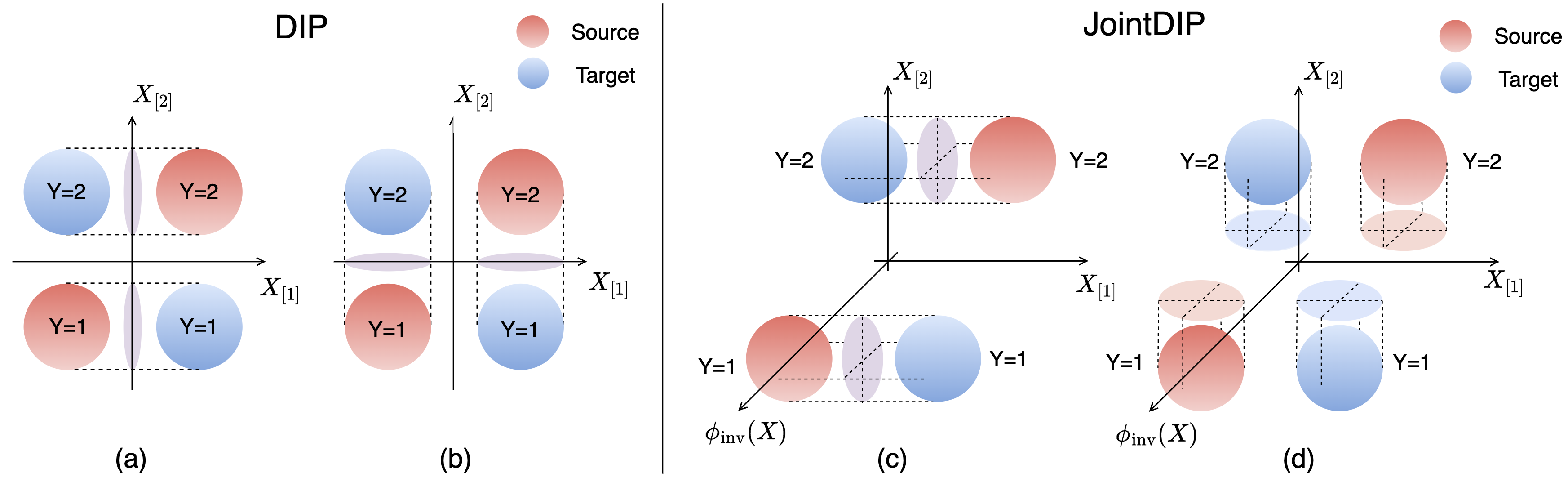
Figure 1: A binary classification example illustrating the difference between DIP and JointDIP. (a) DIP correctly matches the source and target covariates by projecting onto the feature ${X}_{[2]}$, which can generalize to the target distribution. (b) DIP matches the source and target covariates by projecting onto the label-flipping feature ${X}_{[1]}$, which cannot generalize to the target distribution. (c) JointDIP finds the correct feature ${X}_{[2]}$ by jointly matching the covariates with a conditional invariant component (CIC) $\phi_{\textnormal{inv}}(X)$. (d) JointDIP discards the label-flipping feature ${X}_{[1]}$ because the joint distribution of $({X}_{[1]},\phi_{\textnormal{inv}}(X))$ cannot be matched across source and target distributions.

The label-flipping issue in DIP raises concerns about its reliability when applied blindly without additional validation. In the absence of target labels, previous works often rely on assumptions about the data generation process in order for DIP-type of algorithms to achieve low target risk, e.g. linear structural equation models (Chen and Bühlmann, 2020). In this paper, given the availability of multiple source domains, we propose the use of CICs to enhance the reliability of DIP algorithms.

Suppose that we have obtained the conditionally invariant feature mapping $\phi_{\textnormal{inv}}$, and the classifier $h_{\textnormal{inv}}$ built upon CICs denoted by

$$h_{\textnormal{inv}}=g_{\textnormal{inv}}\circ\phi_{\textnormal{inv}}.$$ (27)

As seen in the previous sections, both $\phi_{\textnormal{inv}}$ and $h_{\textnormal{inv}}$ can be approximately obtained by solving CIP—in this case, while finite-sample feature mapping $\widehat{\phi}_{\textnormal{CIP}}$ may not be perfectly conditionally invariant, we expect that they exhibit a small deviation from conditional invariance under the appropriate assumptions, as implied by Proposition 3. Therefore, we assume the exact conditional invariance of $\phi_{\textnormal{inv}}$ for simplicity throughout this section. By leveraging $\phi_{\textnormal{inv}}$ and $h_{\textnormal{inv}}$, we demonstrate that CICs can guide other DA algorithms in two significant ways:

1. Large risk detection: when the classifier $h_{\textnormal{inv}}$ built on CICs has low target risk, it can be used to lower-bound the risk of other DA algorithms, even in the absence of target labels. This enables the identification of label-filpping issues in algorithms like DIP.

2. Joint matching: we propose the JointDIP algorithm which uses CICs $\phi_{\textnormal{inv}}(X)$ to learn invariant features between source and target covariates. JointDIP, as a new DA algorithm, enhances the reliability of DIP by addressing the label-flipping issue often encountered in DIP when the CICs are generic enough.

For the remainder of the section, when a single source is considered, we assume without loss of generality that the first source domain is used.

4.1 Detect failed DA algorithms using CICs

We present the second role of CICs in DA, specifically, in detecting whether another DA classifier has large target risk. Given the conditionally invarinat classifier $h_{\textnormal{inv}}$ as defined in Eq. (27), we prove the following theorem which controls the difference in source and target risks for any classifier.

Theorem 2

Let $h_{\textnormal{inv}}$ be a conditionally invariant classifier and assume that there is no label shift between source and target distributions. For any classifier $h$, its risk difference in source and target is controlled as follows,

$$\left|\mathcal{R}^{{({\mathfrak{T}})}}({h})-\mathcal{R}^{(1)}({h})\right|\leq 2\mathcal{R}^{(1)}({h_{\textnormal{inv}}})\\ +\left|\mathbb{P}\left\{{h(X^{(1)})\neq h_{\textnormal{inv}}(X^{(1)})}\right\}-\mathbb{P}\left\{{h(X^{{({\mathfrak{T}})}})\neq h_{\textnormal{inv}}(X^{{({\mathfrak{T}})}})}\right\}\right|.$$ (28)

This result is proved in Appendix C.1. It shows that a large discrepancy between source and target risks of any classifier $h$ can be detected by examining the source risk of $h_{\textnormal{inv}}$ and the alignments between the predictions of $h$ and $h_{\textnormal{inv}}$ across source and target, which are always available. In practice, we may take $\widehat{h}_{\textnormal{CIP}}$ as a proxy for $h_{\textnormal{inv}}$. By rearranging terms, an empirical version of Eq. (28) can be derived to establish a lower bound for the target risk

$$\mathcal{R}^{{({\mathfrak{T}})}}({h})\geq\widehat{\mathcal{R}}^{(1)}({h})-2\widehat{\mathcal{R}}^{(1)}({\widehat{h}_{\textnormal{CIP}}})\\ -\left|\frac{1}{n^{(1)}}\sum_{k=1}^{n^{(1)}}\mathbf{1}_{{h(X^{(1)}_{k})\neq\widehat{h}_{\textnormal{CIP}}(X^{(1)}_{k})}}-\frac{1}{n^{({\mathfrak{T}})}}\sum_{k=1}^{n^{({\mathfrak{T}})}}\mathbf{1}_{{h(X^{{({\mathfrak{T}})}}_{k})\neq\widehat{h}_{\textnormal{CIP}}(X^{{({\mathfrak{T}})}}_{k})}}\right|.$$ (29)

This lower bound on the target risk can be directly translated to an upper bound on accuracy, which can serve as a certificate to detect the failure of any DA classifier $h$. In Section 5.1.2 and Section 5.2.2, we demonstrate this with numerical examples using CIP to detect the failure of DIP, where we test on both synthetic data and the MNIST dataset. We observe that the accuracy upper bound derived from Eq. (29) to detect the failures of DIP becomes more accurate when CIP has a higher predictive accuracy. If CIP does not perform well across the entire input space, by restricting to a subset of the space where CIP performs well (e.g. region far from decision boundary of a CIP classifier), we can obtain similar results which we will discuss in the subsequent subsection.

4.1.1 Detect large target risk by restricting to a subset

The result of Theorem 2 can be extended in a straightforward manner to the case where we condition on the event $X^{(1)}\in\mathcal{A}$ for any subset $\mathcal{A}\subseteq\mathcal{X}$. Specifically, we write $\mathcal{R}_{{\mathcal{A}}}^{(1)}({h})$ to denote the source risk conditioned on $\mathcal{A}$, i.e.,

$$\mathcal{R}_{{\mathcal{A}}}^{(1)}({h})\coloneqq\mathbb{P}\left\{{h(X^{(1)})\neq Y^{(1)}}\ \middle|\ {X^{(1)}\in\mathcal{A}}\right\},$$

and similarly for the target risk $\mathcal{R}_{{\mathcal{A}}}^{{({\mathfrak{T}})}}({h})$. Analogous to Theorem 2, we can obtain the following bound on the risk difference conditioned on set $\mathcal{A}$.

Corollary 1

Let $h_{\textnormal{inv}}$ be a conditionally invariant classifier and assume that there is no label shift between source and target distributions. For any classifier $h$ and any subset $\mathcal{A}\subseteq\mathcal{X}$, we have

$$\left|\mathcal{R}_{{\mathcal{A}}}^{{({\mathfrak{T}})}}({h})-\mathcal{R}_{{\mathcal{A}}}^{(1)}({h})\right|\leq 2\mathcal{R}_{{\mathcal{A}}}^{(1)}({h_{\textnormal{inv}}})\\ +\left|\mathbb{P}_{{\mathcal{A}}}\left\{{h(X^{(1)})\neq h_{\textnormal{inv}}(X^{(1)})}\right\}-\mathbb{P}_{{\mathcal{A}}}\left\{{h(X^{{({\mathfrak{T}})}})\neq h_{\textnormal{inv}}(X^{{({\mathfrak{T}})}})}\right\}\right|,$$ (30)

where for a random vector $X$, we write

$$\mathbb{P}_{{\mathcal{A}}}\left\{{h(X)\neq h_{\textnormal{inv}}(X)}\right\}\coloneqq\mathbb{P}\left\{{h(X)\neq h_{\textnormal{inv}}(X)}\ \middle|\ {X\in\mathcal{A}}\right\}.$$

From Eq. (30), we can obtain a target risk lower bound for $h$, conditioned on set $\mathcal{A}$, analgous to Eq. (29). If one can identify a region $\mathcal{A}\subseteq\mathcal{X}$ where the classifier $h_{\textnormal{inv}}$ has near perfect source accuracy, due to its conditional invariance, the output of $h_{\textnormal{inv}}$ can serve as a good proxy of the unobserved target labels. One example of such a choice is to choose $\mathcal{A}$ as the region where $h_{\textnormal{inv}}$ gives a high predicted probability. Indeed, our experiments in Section 5.1.2 and Section 5.2.2 compare the tightness of the bounds across the entire space and on a subset $\mathcal{A}$ where $h_{\textnormal{inv}}$ exhibits a high predicted probability. We find that Corollary 1 provides a more accurate estimation of the target risk because $h_{\textnormal{inv}}$ has higher accuracy when constrained to $\mathcal{A}$. In this case, a desired property for $h$ to have a low target risk is to align its output with the output of $h_{\textnormal{inv}}$ on $\mathcal{A}$. We formalize this idea which is a direct consequence of Corollary 1.

Corollary 2

Let $h_{\textnormal{inv}}$ be a conditionally invariant classifier and assume that there is no label shift between source and target distributions. Suppose that $h\in\mathcal{H}$ satisfies

$$h(x)=h_{\textnormal{inv}}(x)\text{ for all $x\in\mathcal{A}$}.$$ (31)

Then the target risk of $h$ on $\mathcal{A}$ is bounded by

$$\mathcal{R}_{{\mathcal{A}}}^{{({\mathfrak{T}})}}({h})\leq 3\mathcal{R}_{{\mathcal{A}}}^{(1)}({h_{\textnormal{inv}}}).$$

In particular, if $h_{\textnormal{inv}}$ has a near perfect accuracy on $\mathcal{A}$ under the source distribution, i.e., $\mathcal{R}_{{\mathcal{A}}}^{(1)}({h_{\textnormal{inv}}})\leq C$ for a small $C\geq 0$, then $\mathcal{R}_{{\mathcal{A}}}^{{({\mathfrak{T}})}}({h})\leq 3C$.

Corollary 2 guarantees the low target population risk of the classifier on the region where the invariant classifier $h_{\textnormal{inv}}$ is confident about its prediction and can serve as a good proxy for the target labels $Y$. This does not necessarily imply that the representation learned via Eq. (31) can generalize to target data outside the region $\mathcal{A}$. Nevertheless, if domain experts all recognize the importance of the region $\mathcal{A}$, Eq. (31) becomes a natural requirement for assessing the quality of any DA classifier.

4.2 JointDIP by matching DIP features jointly with CICs

In this subsection, we demonstrate the third role of CICs in enhancing DIP. According to Theorem 2, if the predictions of $h$ and $h_{\textnormal{inv}}$ align well across source and target, the target risk of $h$ won’t be too far from its source risk. It turns out that we can enforce this alignment by incorporating the CICs into the DIP matching penalty. This leads to our new algorithm, joint domain invariant projection (JointDIP).

Population JointDIP

The population JointDIP minimizes the source risk while matching the joint distributions of $\phi$ and $\phi_{\textnormal{inv}}$ in the representation space across source and target:

$$\begin{split}h_{\textnormal{j-DIP}}&=g_{\textnormal{j-DIP}}\circ\phi_{\textnormal{j-DIP}},\\ g_{\textnormal{j-DIP}},\phi_{\textnormal{j-DIP}}&=\operatorname*{arg\,min}_{g\in\mathcal{G},\phi\in\Phi}\ \ \mathcal{R}^{(1)}({g\circ\phi})\\ &\hskip 14.45377pt\text{subject to }\ \ \mathfrak{D}\left({\mathcal{P}^{(1)}_{{(\phi,\phi_{\textnormal{inv}})(X)}}},{\mathcal{P}^{{({\mathfrak{T}})}}_{{(\phi,\phi_{\textnormal{inv}})(X)}}}\right)=0.\end{split}$$ (32)

Unlike DIP which only matches the marginal distribution of $\phi$, JointDIP takes advantage of CICs to extract invariant feature representations. Intuitively, if $\phi_{\textnormal{inv}}$ is highly correlated with the labels $Y$ and the joint feature mappings $(\phi,\phi_{\textnormal{inv}})$ are marginally invariant, $\phi$ is not likely to learn label-filpping features due to conditional invariance of $\phi_{\textnormal{inv}}$. Note that if label shift is present, it is not hard to extend the current formulation to an importance-weighted JointDIP (IW-JointDIP) by applying CIP to correct label shift prior to applying JointDIP.

Finite-sample JointDIP

The finite sample formulation of JointDIP enforces the joint invariance of the representations via a regularization term,

$$\begin{split}\widehat{h}_{\textnormal{j-DIP}}&=\widehat{g}_{\textnormal{j-DIP}}\circ\widehat{\phi}_{\textnormal{j-DIP}},\\ \widehat{g}_{\textnormal{j-DIP}},\widehat{\phi}_{\textnormal{j-DIP}}&=\operatorname*{arg\,min}_{g\in\mathcal{G},\phi\in\Phi}\ \ \widehat{\mathcal{R}}^{(1)}({g\circ\phi})+\lambda_{\textnormal{j-DIP}}\cdot\mathfrak{D}\left({\widehat{\mathcal{P}}^{(1)}_{{(\phi,\phi_{\textnormal{inv}})(X)}}},{\widehat{\mathcal{P}}^{{({\mathfrak{T}})}}_{{(\phi,\phi_{\textnormal{inv}})(X)}}}\right),\end{split}$$ (33)

where $\lambda_{\textnormal{j-DIP}}>0$ is a regularization parameter that controls the strength of the joint matching penalty.

To illustrate the advantage of JointDIP over the ordinary DIP, consider a binary classification example under the general anticausal model Definition 4 where the data is generated as in Figure 1 (a)(b), similar to the example in Johansson et al. (2019). Suppose that $\Phi=\{\phi_{1}(x)={x}_{[1]},\phi_{2}(x)={x}_{[2]}\}$ and $\mathcal{G}=\{g_{a}(z)=\mathbf{1}_{{z>a}}+1,a\in\real\}$. Since DIP only matches the marginal distributions in the representation space, it could choose either $\phi_{1}$ or $\phi_{2}$ as the feature mappings to perfectly match the marginal distributions of the features and achieve zero loss under the source distribution. However, choosing $\phi_{1}$ leads to zero accuracy under the target distribution, as $\phi_{1}(X)={X}_{[1]}$ is the label-flipping feature. Only $\phi_{2}(X)={X}_{[2]}$ is the conditionally invariant feature that can generalize to the target distribution. Now if we have access to CICs through the conditionally invariant feature mapping $\phi_{\textnormal{inv}}$, and we match these jointly with DIP, we would only get the correct feature $\phi_{2}(X)={X}_{[2]}$, as illustrated in Figure 1 (c)(d). JointDIP would never select $\phi_{1}(X)={X}_{[1]}$ because the joint distribution of $({X}_{[1]},\phi_{\textnormal{inv}}(X))$ is different between the source and target distributions.

4.2.1 Theoretical comparison of CIP, DIP, and JointDIP under general anticausal model

To quantitatively compare the target risk of DA classifiers, we focus on data generated from the general anticausal model defined in Definition 4. Additionally, we introduce Assumption 3 where marginal distribution of $Y$ is uniform under source and target distributions, as follows.

Assumption 3

Suppose that data is generated according to the general anticausal model defined in Definition 4. Further, assume that the label distribution is uniform under source and target distributions, i.e.,$\forall m\in\{1,2,\ldots,M\}$ and $\forall y\in\{1,2,\ldots,L\}$, we have ${p^{{(m)}}_{y}}={p^{{({\mathfrak{T}})}}_{y}}=1/L$.

With the above assumptions on the data generation process in place, the following theorem compares the target risk of population CIP, DIP, and JointDIP.

Theorem 3

Suppose that source and target data are generated under Assumption 3. Let $\Phi=\{\phi(x)=Ax+b,A\in{}^{q\times p},b\in{}^{q}\}$ be the class of linear feature mapping from $\mathbb{R}^{p}$ to $\mathbb{R}^{q}$, which is used in the optimization of population DIP (11) and population JointDIP (32). Assume that both algorithms match feature distributions exactly, i.e.,

$$\mathcal{P}^{(1)}_{{\phi_{\textnormal{DIP}}(X)}}=\mathcal{P}^{{({\mathfrak{T}})}}_{{\phi_{\textnormal{DIP}}(X)}}\text{ and }\mathcal{P}^{(1)}_{{(\phi_{\textnormal{j-DIP}},\phi_{\textnormal{inv}})(X)}}=\mathcal{P}^{{({\mathfrak{T}})}}_{{(\phi_{\textnormal{j-DIP}},\phi_{\textnormal{inv}})(X)}}.$$

Then the following statements hold:

1. There exist distributions $\mathcal{P}^{(1)},\mathcal{P}^{{({\mathfrak{T}})}}$ such that the feature mapping of population DIP, $\phi_{\textnormal{DIP}}$, flips the labels after matching the marginal distributions in the representation space, i.e.,

   $$\mathcal{P}^{(1)}_{{\phi_{\textnormal{DIP}}(X)}|{Y=y}}=\mathcal{P}^{{({\mathfrak{T}})}}_{{\phi_{\textnormal{DIP}}(X)}|{Y=\pi(y)}},\ \ \forall y\in\{1,\ldots,L\},$$ (34)

   for some permutation $\pi\neq\mathbf{I}$ over $\mathcal{Y}$.

2. Suppose $\phi_{\textnormal{inv}}:{}^{p}\rightarrow{}^{r}$ is a linear conditionally invariant feature mapping such that

   $$\mathbb{E}\left[{\phi_{\textnormal{inv}}(X^{(1)})}\ \middle|\ {Y^{(1)}=i}\right]\neq\mathbb{E}\left[{\phi_{\textnormal{inv}}(X^{(1)})}\ \middle|\ {Y^{(1)}=j}\right],\ \ \forall i\neq j\in\mathcal{Y}.$$ (35)

   Then the feature mapping of population JointDIP, $\phi_{\textnormal{j-DIP}}$, is conditionally invariant across $\mathcal{P}^{(1)}$ and $\mathcal{P}^{{({\mathfrak{T}})}}$. If additionally $r\leq q$, then the target risk of JointDIP is no greater than that of the optimal classifier built on $\phi_{\textnormal{inv}}^{0}\coloneqq\begin{pmatrix}\phi_{\textnormal{inv}},\mathbf{0}_{q-r}\end{pmatrix}$, i.e.,

   $$\mathcal{R}^{{({\mathfrak{T}})}}({h_{\textnormal{j-DIP}}})\leq\min_{g\in\mathcal{G}}\mathcal{R}^{{({\mathfrak{T}})}}({g\circ\phi_{\textnormal{inv}}^{0}}),$$

   and when $\phi_{\textnormal{inv}}=\phi^{\star}$, we have $\mathcal{R}^{{({\mathfrak{T}})}}({h_{\textnormal{j-DIP}}})\leq\mathcal{R}^{{({\mathfrak{T}})}}({h^{\star}})$.

3. Suppose $\phi_{\textnormal{inv}}:{}^{p}\rightarrow{}^{r}$ is a conditionally invariant feature mapping such that the matrix

   $$C_{\phi_{\textnormal{inv}}}(a)=\begin{pmatrix}1&1&\cdots&1\\ m_{1}^{1}(a)&m_{2}^{1}(a)&\cdots&m_{L}^{1}(a)\\ \vdots&\vdots&\ddots&\vdots\\ m_{1}^{L-1}(a)&m_{2}^{L-1}(a)&\cdots&m_{L}^{L-1}(a)\end{pmatrix}\in{}^{L\times L},$$ (36)

   is full rank for some vector $a\in{}^{r}$, where $m_{j}^{\ell}(a)=\mathbb{E}\left[{\left(a^{\top}\phi_{\textnormal{inv}}(X^{(1)})\right)^{\ell}}\ \middle|\ {Y^{(1)}=j}\right]$. Then the feature mapping of population JointDIP, $\phi_{\textnormal{j-DIP}}$, is conditionally invariant across $\mathcal{P}^{(1)}$ and $\mathcal{P}^{{({\mathfrak{T}})}}$.

The proof of this result is given in Appendix C.2. The proofs for Theorem 3(a) and Theorem 3(b) rely on the matching property of the two mixing distributions, whereas the proof for Theorem 3(c) analyzes distribution matching in the space of characteristic functions. Theorem 3(a) shows that while DIP uses the additional target covariates information, the corresponding representations can fail to satisfy conditional invariance across source and target distributions; and in fact, if the features correspond to the label-flipping features, as illustrated in Figure 1, it can potentially hurt the target prediction performance.

By contrast, Theorem 3(b) shows that when $\phi_{\textnormal{inv}}$ is a linear conditionally invariant feature mapping, the features obtained by JointDIP are conditionally invariant across $\mathcal{P}^{(1)}$ and $\mathcal{P}^{{({\mathfrak{T}})}}$, therefore avoiding the label-flipping issue of DIP. The condition (35) requires that conditional means of $\phi_{\textnormal{inv}}$ are different for any pair of labels $i$ and $j$. This condition is a reasonable expectation for any $\phi_{\textnormal{inv}}$ exhibiting a good prediction performance as otherwise there is no way for classifiers built on $\phi_{\textnormal{inv}}$ to distinguish between labels $i$ and $j$. See Appendix A.2 for an example of the general anticausal model that satisfies the condition (35). Additionally, Theorem 3(b) assures that JointDIP cannot be worse than the optimal classifier built upon $\phi_{\textnormal{inv}}$. This result is expected because CICs tend to be conservative. For instance, CICs identified via CIP are forced to be conditionally invariant across $M$ many source distributions (and ideally the target distribution), which can potentially eliminate features that are useful for predicting target labels. JointDIP addresses this issue by seeking conditional invariant representations across a single source and target domains to construct a more effective classifier than one solely based on CICs.

Finally, for any conditionally invariant feature mapping $\phi_{\textnormal{inv}}$ which may not necessarily be linear, Theorem 3(c) guarantees that the features obtained by JointDIP are conditionally invariant across $\mathcal{P}^{(1)}$ and $\mathcal{P}^{{({\mathfrak{T}})}}$, as long as the matrix $C_{\phi_{\textnormal{inv}}}(a)$ given in Eq. (36) is full rank. The matrix $C_{\phi_{\textnormal{inv}}}(a)$ is full rank if the CICs under different labels are in a generic position. Comparing with the condition (35) in the linear case, this condition may be more difficult to verify generally as it requires computation of higher order moments. We provide concrete examples in Appendix A.3 where this condition is satisfied. In practice, we can either use $\widehat{\phi}_{\textnormal{CIP}}$ as $\phi_{\textnormal{inv}}$, or refer to domain experts for suggestions on reasonable CICs.

5 Numerical experiments

In this section, we investigate the target performance of our proposed DA algorithms and compare them with existing methods. In particular, we demonstrate through our experiments the effectiveness of the importance-weights correction in the presence of both covariate and label distribution shifts, the capability of detecting DIP’s failure using estimated CICs, and the superior performance of JointDIP over DIP when label-flipping features are present. We consider DA classification tasks across four datasets: synthetic data generated from linear Structral Causal Models (SCMs), the MNIST data (LeCun, 1998) under rotation intervention, the CelebA data (Liu et al., 2015) under color intervention, and the Camelyon17 data from WILDS (Koh et al., 2021; Sagawa et al., 2021). Except for the Camelyon17 data, the domain shifts in other datasets are synthetically created.

We conduct a thorough comparative analysis where our methods are benchmarked against various DA algorithms. In addition to DIP, CIP, IW-CIP, and JointDIP which have been introduced in previous sections, we additionally explore several variants of these algorithms, including IW-DIP and IW-JointDIP. IW-DIP is the algorithm that applies CIP for importance weighting to correct label shift prior to DIP, while IW-JointDIP applies this importance weighting step before JointDIP. Moreover, for ERM, DIP, and JointDIP, we consider both their single-source versions (e.g. DIP) and their multi-source versions (e.g. DIP-Pool). In terms of distributional distances, both squared mean distance and Maximum Mean Discrepancy (MMD) are considered. Lastly, we compare these methods with existing well-known DA algorithms such as Invariant Risk Minimization (IRM) (Arjovsky et al., 2019), V-REx (Krueger et al., 2021), and groupDRO (Sagawa et al., 2019). A detailed description of each DA algorithm, models architectures, and the training setup are presented in Appendix D.

Certain DA algorithms, such as DIP or IW-DIP, rely on a single source domain to learn invariant feature representations and construct the final classifiers (see Appendix D). In this work, we do not focus on how to choose the best single source domain for these algorithms, but instead simply select the last source domain. By design, this single source domain is usually similar to the target domain in terms of the considered covariate shifts, such as mean shift (linear SCMs), rotation angle (MNIST), and color balance (CelebA). However, this domain may have label-flipping features compared to the target domain. We delibrately design these settings to demonstrate that, under such settings, DIP might induce label flipping, while JointDIP avoids this issue.

5.1 Linear structural causal models (SCMs)

We perform experiments on synthetic datasets generated according to linear SCMs under the general anticausal model defined in Definition 4. We first compare the performance of various DA methods, and then show how to use CICs to detect the failure of DIP without access to target labels.

5.1.1 Linear SCMs under different interventions

We consider three different types of domain shifts: mean shift, label shift, and a shift to introduce label-flipping features. In all SCMs, we introduce the mean shift across domains. Depending on the presence or absence of label shift and the shift that introduces label-flipping features, we obtain four combinations and their corresponding SCMs. We use $M^{\prime}=M+1$ to denote the total number of source and target domains. The last source domain (the $M$-th domain) is always set as the single source domain for DA algorithms which utilize only one source domain (e.g. DIP). The last domain (the $M^{\prime}$-th domain) serves as the target domain, and we generate 1000 samples per domain. Instead of specifying each $f^{(m)}(\cdot)$ and $f^{{({\mathfrak{T}})}}(\cdot)$ in Definition 4, we provide explicit representations of the data generation model for each SCM. For simplicity, we only present the data generation model for source data, and the target data generation model can be obtained by replacing the superscript $(m)$ with ${({\mathfrak{T}})}$.

• SCM i@: mean shift exists; no CICs; no label shift; no label-flipping features; $M^{\prime}=4$ and $p=10$. The data generation model is

  $$Y^{(m)} \sim\text{Bernoulli}(0.5),$$

  $$X^{(m)} =0.2Y\cdot\mathds{1}_{10}+0.25\cdot\mathcal{N}(0,\mathbb{I}_{10})+A^{(m)},$$

  where $\mathds{1}_{10}\in\mathbb{R}^{10}$ denotes a vector consisting of ones and $\mathbb{I}_{10}\in\mathbb{R}^{10\times 10}$ denotes the identity matrix. For all source domains, the mean shift $A^{(m)}$, $1\leq m\leq M$, is generated by $0.2\cdot\mathcal{N}(0,\mathbb{I}_{10})$, while the target domain suffers a large intervention $A^{({\mathfrak{T}})}\sim 2\cdot\text{sign}\left(\mathcal{N}(0,\mathbb{I}_{10})\right)$. Note that we do not introduce any CICs in SCM i@. This allows us to examine the most extreme case of mean shift where all coordinates of $X$ are perturbed. However, in the following three SCMs (SCM ii@, iii@, and iv@), we ensure the presence of CICs and expect that certain DA algorithms can exploit these CICs.

• SCM ii@: mean shift exists; CICs exist; label shift exists; no label-flipping features; $M^{\prime}=12$ and $p=9$. The data generation model is

  $$Y^{(m)} \sim\text{Bernoulli}(p^{(m)}),$$

  $$X^{(m)}_{[1:6]} =0.2(Y^{(m)}-0.5)\cdot\mathds{1}_{6}+0.25\cdot\mathcal{N}(0,\mathbb{I}_{6})+A^{(m)},$$

  $$X^{(m)}_{[7:9]} =0.2(Y^{(m)}-0.5)\cdot\mathds{1}_{3}+0.25\cdot\mathcal{N}(0,\mathbb{I}_{3}),$$

  where the label distribution $p^{(m)}=0.5$, for $1\leq m\leq M,$ is balanced in source domains but perturbed in target domain with $p^{{({\mathfrak{T}})}}=0.1$. The mean shift only exists in the first six coordinates of $X$, where $A^{(m)}$, $1\leq m\leq M$ is generated by $\mathcal{N}(0,\mathbb{I}_{6})$ in the source domains, while the target domain suffers a large intervention $A^{({\mathfrak{T}})}\sim 2\cdot\text{sign}\left(\mathcal{N}(0,\mathbb{I}_{6})\right)$. The last three coordinates of $X$ remain unperturbed and they serve as CICs.

• SCM iii@: mean shift exists; CICs exist; no label shift; label-flipping features exist; $M^{\prime}=12$ and $p=18$. The data generation model is

  $$Y^{(m)} \sim\text{Bernoulli}(0.5),$$

  $$X^{(m)}_{[1:6]} =0.3(Y^{(m)}-0.5)\cdot\mathds{1}_{6}+0.4\cdot\mathcal{N}(0,\mathbb{I}_{6})+A^{(m)},$$

  $$X^{(m)}_{[7:12]} =\begin{cases}0.3(0.5-Y^{(m)})\cdot\mathds{1}_{6}+0.1\cdot\mathcal{N}(0,\mathbb{I}_{6}),&$m$\text{ is odd},\\ 0.3(Y^{(m)}-0.5)\cdot\mathds{1}_{6}+0.1\cdot\mathcal{N}(0,\mathbb{I}_{6}),&$m$\text{ is even},\end{cases}$$

  $$X^{(m)}_{[13:18]} =0.3(Y^{(m)}-0.5)\cdot\mathds{1}_{6}+0.4\cdot\mathcal{N}(0,\mathbb{I}_{6}),$$

  The first six coordinates of $X$ suffer mean shift, with $A^{(m)}$, $1\leq m\leq M$ and $A^{({\mathfrak{T}})}\sim\mathcal{N}(0,\mathbb{I}_{d})$ across all domains. In particular, we make the last source domain and target domain share similar mean shift interventions: $A^{(11)}=a_{0}+a_{1}$ and $A^{(12)}=a_{0}+a_{2}$, where $a_{0}\sim 0.8\cdot\mathcal{N}(0,\mathbb{I}_{6})$ and $a_{1},a_{2}\sim 0.6\cdot\mathcal{N}(0,\mathbb{I}_{6})$. This setting potentially enables DIP-based methods to better rely on the last source domain because of the similarity of ${X}_{[1:6]}$ between this domain and the target domain. However, the $7^{\text{th}}$ to $12^{\text{th}}$ coordinates of $X$ are label-flipping features according to Definition 3: in the first six domains ${X}_{[7:12]}$ has positive correlation with $Y$, while the correlation is negative in the remaining six domains, including the target domain. There is no interventions on the last six coordinates of $X$, and they serve as CICs.

• SCM iv@: mean shift exists; CICs exist; label shift exists; label-flipping features exist, $M^{\prime}=12$ and $p=18$. The data generation model of $X\mid Y$ is the same as SCM iii@, but we additionally perturb the marginal distribution of $Y$ across source and target distributions. Specifically, the label distribution $Y^{(m)}\sim\text{Bernoulli}(0.5)$ is balanced in source domains but perturbed in target domain with $Y^{{({\mathfrak{T}})}}\sim\text{Bernoulli}(0.3)$.

	SCM i@		SCM ii@		SCM iii@		SCM iv@
Mean shift	Y		Y		Y		Y
CICs	N		Y		Y		Y
Label shift	N		Y		N		Y
Label-flipping features	N		N		Y		Y
DA Algorithm	src_acc	tar_acc	src_acc	tar_acc	src_acc	tar_acc	src_acc	tar_acc
Tar	70.6$\pm$13.8	89.0$\pm$0.7	69.4$\pm$3.9	92.9$\pm$1.0	70.1$\pm$2.9	97.9$\pm$0.4	69.8$\pm$3.0	96.9$\pm$0.7
ERM	89.6$\pm$1.0	56.1$\pm$12.0	87.5$\pm$1.0	57.4$\pm$33.3	97.9$\pm$0.3	58.9$\pm$5.0	98.0$\pm$0.3	58.7$\pm$10.7
ERM-Pool	88.3$\pm$2.3	54.4$\pm$10.2	78.5$\pm$1.3	58.6$\pm$29.3	83.3$\pm$0.8	75.3$\pm$7.7	83.3$\pm$0.7	78.9$\pm$6.8
DIP	88.3$\pm$1.0	87.6$\pm$1.5	84.5$\pm$3.1	62.0$\pm$2.9	93.5$\pm$3.4	34.5$\pm$14.9	94.4$\pm$2.7	35.3$\pm$14.6
DIP-Pool	86.7$\pm$2.8	86.4$\pm$2.2	75.8$\pm$0.7	60.1$\pm$3.1	84.1$\pm$0.5	82.0$\pm$1.1	84.4$\pm$0.5	82.3$\pm$3.8
CIP	87.4$\pm$3.3	55.9$\pm$12.0	75.2$\pm$0.7	75.7$\pm$6.5	82.2$\pm$0.4	81.8$\pm$1.3	82.2$\pm$0.4	82.1$\pm$1.2
IW-ERM	54.8$\pm$11.6	52.4$\pm$10.4	59.3$\pm$9.6	54.1$\pm$37.7	80.3$\pm$9.1	75.1$\pm$8.9	77.2$\pm$9.0	79.2$\pm$4.8
IW-CIP	53.7$\pm$9.9	54.0$\pm$11.8	50.3$\pm$0.7	90.4$\pm$0.8	82.5$\pm$0.4	81.2$\pm$4.1	81.0$\pm$0.9	83.8$\pm$2.2
IW-DIP	56.2$\pm$12.8	54.3$\pm$11.7	71.1$\pm$10.8	92.1$\pm$2.7	88.4$\pm$13.0	37.2$\pm$14.9	83.7$\pm$8.6	64.2$\pm$7.3
JointDIP	87.1$\pm$1.3	86.8$\pm$1.9	82.8$\pm$2.7	70.6$\pm$6.2	88.8$\pm$1.3	85.4$\pm$2.1	88.6$\pm$1.9	82.8$\pm$1.9
IW-JointDIP	68.4$\pm$19.1	68.0$\pm$19.4	51.7$\pm$3.9	90.0$\pm$1.3	87.8$\pm$1.5	82.9$\pm$8.1	84.1$\pm$3.4	85.1$\pm$3.7
IRM	87.6$\pm$2.2	56.7$\pm$10.4	70.9$\pm$2.5	71.9$\pm$17.9	80.1$\pm$1.8	80.2$\pm$1.8	84.2$\pm$0.6	83.7$\pm$3.3
V-REx	87.3$\pm$2.5	55.6$\pm$11.5	77.9$\pm$1.2	62.9$\pm$25.7	83.8$\pm$0.8	80.4$\pm$7.6	84.3$\pm$0.6	83.8$\pm$3.7
groupDRO	88.3$\pm$2.3	54.4$\pm$10.0	77.8$\pm$1.1	64.2$\pm$25.7	84.0$\pm$0.7	81.3$\pm$7.4	83.9$\pm$0.6	84.3$\pm$3.2

Table 1: Source and target accuracy in linear SCMs under different interventions. For each setting of SCM, DA algorithms are run on 10 different datasets, each generated using 10 different random seeds. Tar represents the oracle method where the model is trained on the labeled target data. The top four methods are highlighted in bold. The best method (excluding Tar) is colored in red.

We use a linear model in all SCM experiments to predict the labels; see Appendix D.2 for details. Table 1 compares the target performance of different DA algorithms. In SCM i@ where only mean shift exists and no CICs exist, DIP gives the best performance, with JointDIP showing comparable accuracy. ERM and other DA algorithms which aim to find invariance across all source domains (e.g. CIP, IRM, V-REx) fail to generalize to the target domain due to the lack of CICs and the substantial mean shift in the target domain. In SCM ii@ where mean shift exists and label shift is added as another intervention, IW-DIP achieves the highest accuracy. Both IW-CIP and IW-JointDIP also achieve over 90% correct predictions. However, IW-ERM which directly applies importance weighting without using CICs completely fails, indicating that identifying conditionally invariant features before applying label correction is necessary in this scenario.

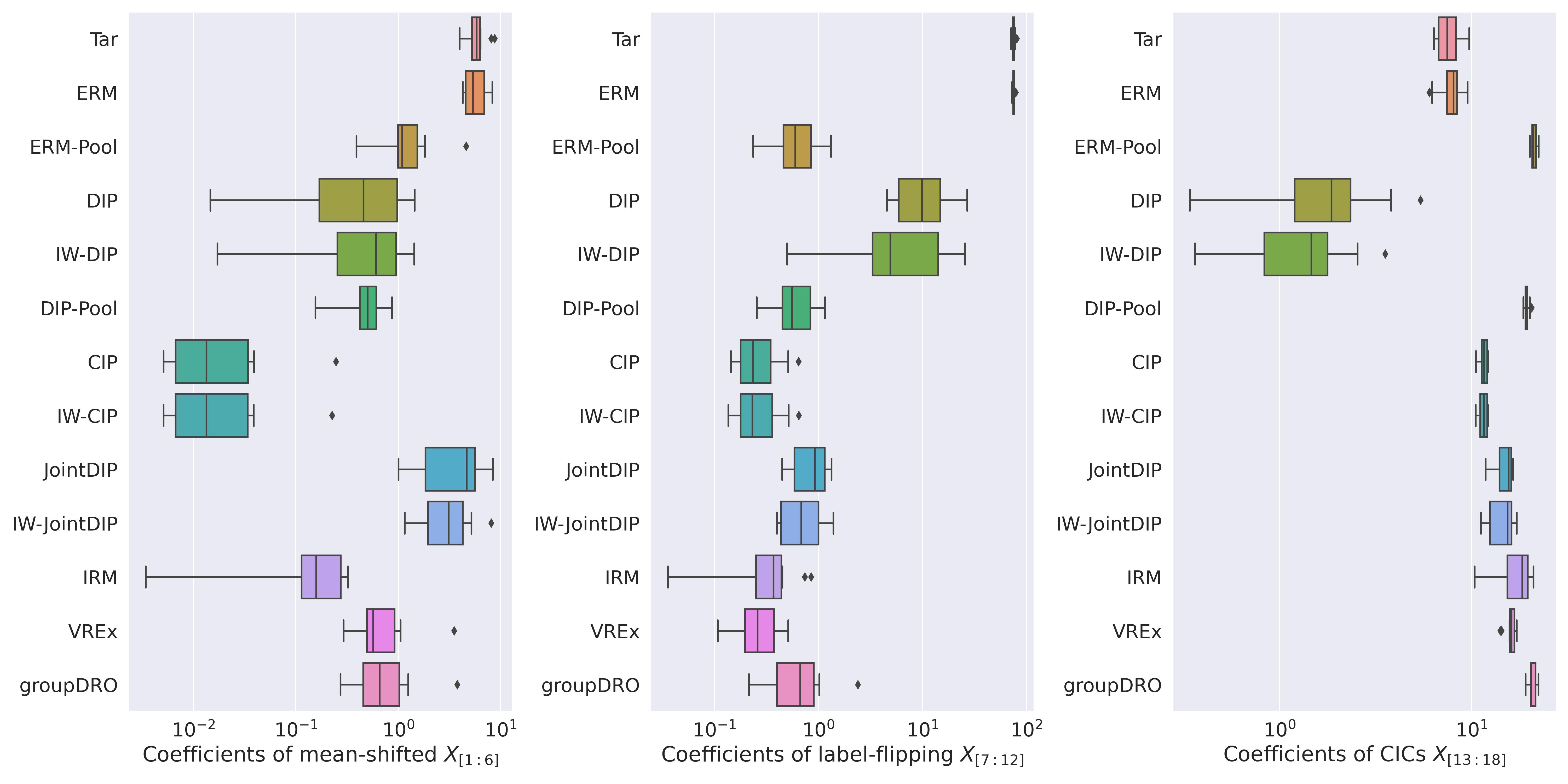
Figure 2: $L^{1}$ norm of coefficients in SCM iii@. Coefficients are grouped into three categories, depending on how corresponding coordinates are perturbed. Contrary to DIP, JointDIP does not have large coefficients on label-flipping features, demonstrating that JointDIP can avoid label-flipping issue observed in DIP.

In SCM iii@ where label-flipping features exists, we observe that DIP results in an accuracy lower than a random guess. On the contrary, JointDIP achieves the highest accuracy. To gain a deeper understanding of the classifiers obtained by each algorithm, in Figure 2 we illustrate the $L^{1}$ norm of the coefficients of three categories of coordinates: mean-shifted ${X}_{[1:6]}$, label-flipping ${X}_{[7:12]}$, and CICs ${X}_{[13:18]}$. Three key observations can be made from the figure: First, DIP shows large coefficients on the label-flipping features ${X}_{[7:12]}$, providing insight for its suboptimal performance. Second, DA methods that seek invariant features across all source domains, such as CIP, IRM, V-REx, show small coefficients on both the mean-shifted features and label-flipping features, but large coefficients on the CICs. This result aligns with their fundamental objective of identifying invariant representations across source domains. Lastly, JointDIP demonstrates small coefficients on label-flipping features, but relatively larger coefficients on mean-shifted coordinates, confirming that JointDIP effectively discards label-flipping features ${X}_{[7:12]}$, retains some of the invariant features ${X}_{[13:18]}$ identified by CIP while exploiting the useful mean-shifted features ${X}_{[1:6]}$.

Lastly in SCM iv@ where mean shift, label shift, and label flipping features exist simultaneously, we find that IW-JointDIP outperforms other methods in the target accuracy. This can be attributed to its three step approach—first finding CICs, then correcting label shift via CICs, and finally aligning potential features via JointDIP—which effectively addresses the combination of these three shifts.

Overall, our experiments across various SCM settings reveal that while traditional DA methods like CIP and DIP may struggle with certain types of shifts, JointDIP excels in handling label-flipping features, and importance-weighted variants of the DA methods perform well in scenarios with label shift.

5.1.2 Detecting failure of DIP in linear SCMs

Previously in Section 4.1, we discussed the second role of CICs to detect the failure of DA algorithms without requiring access to target labels. To demonstrate this second role in practice, here we apply Theorem 2 and Corollary 1 to DIP and JointDIP within the context of SCM iii@. We take the finite-sample CIP as $\phi_{\textnormal{inv}}$, and compare the accuracy upper bound derived from Theorem 2 against the actual accuracy of DIP and JointDIP as shown in Figure 3 (a)(b). We vary the DIP penalty parameter in DIP and the JointDIP penalty parameter in JointDIP (both represented by $\lambda$). The CIP penalty parameter utilized in CIP and JointDIP is set to the optimal value found via hyperparmeter search. The figure illustrates that while the accuracy upper bound from Theorem 2 is valid, it exceeds the true accuracy by a wide margin, which is undesirable. Consequently, it is difficult to directly apply Theorem 2 to test the failure of DIP in SCM iii@.

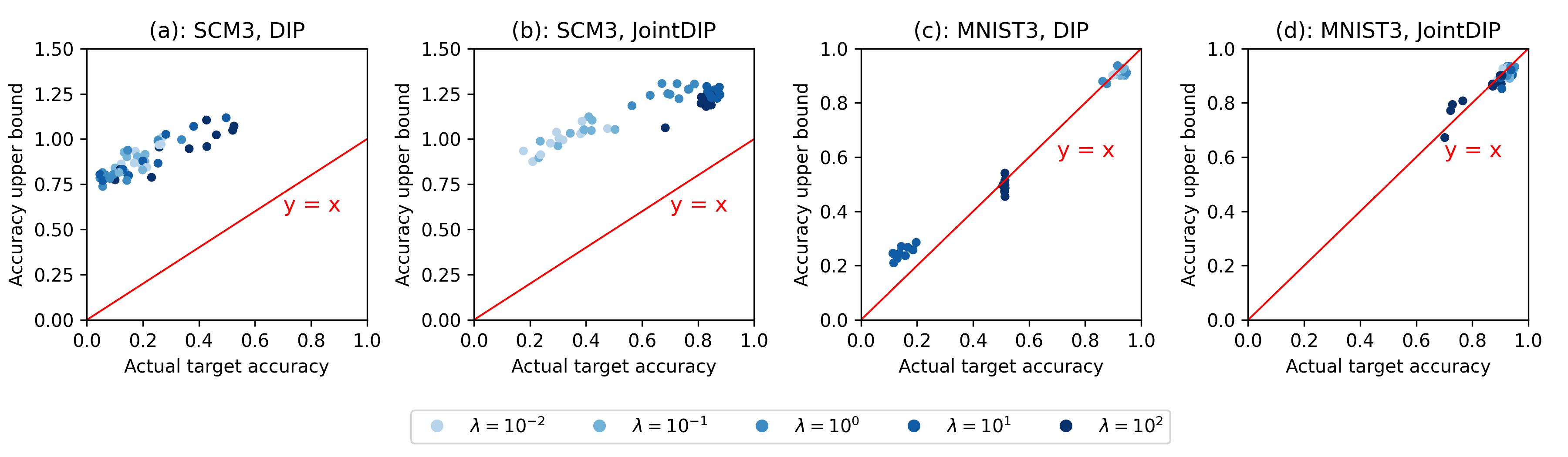
Figure 3: SCM iii@ and MNIST iii@: target accuracy upper bound obtained via Theorem 2 vs. actual target accuracy. For SCM iii@, the accuracy of CIP is low, resulting in an upper bound that does not provide a tight estimation of the true target accuracy for both DIP and JointDIP. Conversely, in MNIST iii@, CIP achieves high accuracy and the accuracy upper bound precisely reflects the true target accuracy. The red line indicates $y=x$.

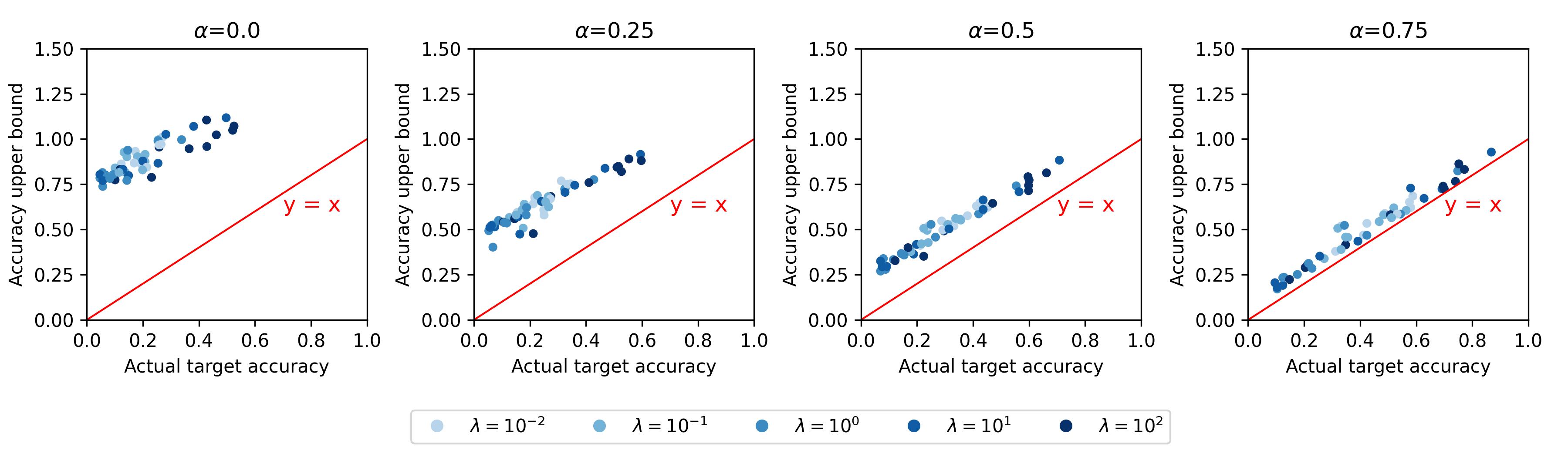
Figure 4: DIP in SCM iii@: target accuracy upper bound obtained via Corollary 1 vs. actual target accuracy in region $\mathcal{A}$. We define region $\mathcal{A}$ as $\mathcal{A}=Q_{\alpha}\coloneqq\{X\in\mathcal{X}\mid\text{CIP predicted probability}\geq q_{\alpha}\}$, where $q_{\alpha}$ is the threshold such that $(1-\alpha)\times 100\%$ of target covariates have a CIP predicted probability greater than $q_{\alpha}$. The larger $\alpha$ is, the more confident CIP is about the prediction on the covariate samples in $Q_{\alpha}$. The red line indicates $y=x$.

We then turn to apply Corollary 1 to compare the accuracy upper bound with the actual accuracy of DIP within region $\mathcal{A}$, where we define $\mathcal{A}$ as the region such that the CIP predicted probability exceeds a threshold $q_{\alpha}$. This threshold $q_{\alpha}$ is defined as the $\alpha\times 100$-th percentile of CIP predicted probability for the target covariates, i.e., $(1-\alpha)\times 100\%$ of target covariates have a CIP predicted probability greater than $q_{\alpha}$. As shown in Figure 4, by increasing $\alpha$, we observe that our upper bound becomes increasingly precise within region $\mathcal{A}$. For example, DIP with certain values of $\lambda$ yields an upper bound lower than 0.5, suggesting that DIP flips the label. Although a low accuracy within region $\mathcal{A}$ does not necessarily translate to low accuracy across the entire target domain, in practice we can refer to domain experts and ask them whether such suboptimal performance of DIP within region $\mathcal{A}$ is reasonable or not, allowing us to avoid the need to acquire and validate all target labels.

5.2 MNIST under rotation intervention

In this section, we consider binary classification of the MNIST dataset (LeCun, 1998) under rotation interventions, where digits 0-4 are categorized as label 0 and digits 5-9 are categorized as label 1. Similar to our experiments in SCMs, we first evaluate the prediction performance of various DA methods, then discuss how to detect potential failure of DIP without requiring access to target labels.

Figure 5: Sample images from MNIST iii@. In this dataset, two different types of interventions have been applied: a rotation shift and the inclusion of label-flipping features. For rotation shift, each image in the $m$-th domain is rotated clockwise by $(m\times 15-30)^{\circ}$. As for the label-flipping features, a white bar of $6\times 16$ pixels is added at the bottom-left corner of the images. The correlation between the label and the white bar patch changes across the domains, with positive correlation in the $1^{\text{st}},3^{\text{rd}}$, and $5^{\text{th}}$ domains, and negative correlation in the $2^{\text{nd}},4^{\text{th}}$, and $6^{\text{th}}$ (target) domains.

5.2.1 Rotated MNIST under different interventions

We create five source domains and one target domain (the $6^{\text{th}}$ domain). The $5^{\text{th}}$ domain is fixed as the single source domain for DA algorithms that rely on only one source domain. Each source domain consists of 20% of the images from the MNIST training set, and the target domain includes all images from the MNIST test set. We introduce three different types of interventions as follows:

• Rotation shift: Each image in the $m$-th domain is rotated clockwise by $(m\times 15-30)^{\circ}$.

• Label shift: In the target domain, we remove $50\%$ of the images labelled as 0.

• Label-flipping features: In the $1^{\text{st}},3^{\text{rd}}$, and $5^{\text{th}}$ domains, $90\%$ of the images with label 1 and $10\%$ of the images with label 0 are patched by a white bar of $6\times 16$ pixels at the bottom-left corner. This creates a correlation of $0.8$ between the label and the patch. Conversely, in the $2^{\text{nd}},4^{\text{th}}$, and $6^{\text{th}}$ domains, we add this white bar to $90\%$ of the images with label 0 and $10\%$ of the images with label 1. This creates a correlation of $-0.8$ between the label and the patch.

Similar to the settings of SCMs, we consider four DA problems under different combinations of these interventions. The rotation shift intervention is applied to all MNIST experiments, and four different cases are constructed based on whether the label shift or label-flipping features exist: MNIST i@ includes rotation shift, but does not have label shift and label-flipping features; MNIST ii@ includes rotation shift and label shift, but does not have label-flipping features; MNIST iii@ includes rotation shift and label-flipping features, but does not have label shift; and MNIST iv@ includes all three interventions—rotation shift, label shift, and the presence of label-flipping feature. Image samples under MNIST iii@ are displayed in Figure 5 for illustration.

We train a Convolutional Neural Network (CNN) model similar to LeNet5 (LeCun et al., 1998) for all MNIST experiments; see Appendix D.2 for more details. Table 2 summarizes the performance of various DA methods on MNIST. Similar to our findings in linear SCM experiments, we conclude that DIP effectively addresses rotation shift in the absence of label-flipping features (MNIST i@), while label correction addresses label shift (MNIST ii@ and iv@), and JointDIP mitigates the issue of learning label-flipping features for DIP (MNIST iii@ and iv@). Consequently, DA methods which incorporate steps specifically designed to address each shift have the best performance or are among the top-performing methods.

	MNIST i@		MNIST ii@		MNIST iii@		MNIST iv@
Rotation shift	Y		Y		Y		Y
Label shift	N		Y		N		Y
Label-flipping features	N		N		Y		Y
DA Algorithm	src_acc	tar_acc	src_acc	tar_acc	src_acc	tar_acc	src_acc	tar_acc
Tar	71.2$\pm$0.9	100.0$\pm$0.0	69.3$\pm$1.5	99.7$\pm$0.3	67.4$\pm$1.1	100.0$\pm$0.1	66.2$\pm$1.9	99.9$\pm$0.1
ERM	99.9$\pm$0.1	96.9$\pm$0.4	99.9$\pm$0.2	96.9$\pm$0.5	100.0$\pm$0.1	87.8$\pm$1.9	100.0$\pm$0.1	86.8$\pm$1.8
ERM-Pool	99.5$\pm$0.4	94.6$\pm$0.8	99.5$\pm$0.3	94.6$\pm$1.3	99.4$\pm$0.5	88.7$\pm$2.0	99.6$\pm$0.2	89.1$\pm$2.5
DIP	100.0$\pm$0.1	97.5$\pm$0.3	99.9$\pm$0.2	96.7$\pm$0.5	100.0$\pm$0.0	91.0$\pm$1.9	100.0$\pm$0.0	90.1$\pm$1.6
DIP-Pool	99.6$\pm$0.2	95.7$\pm$0.4	99.6$\pm$0.2	94.6$\pm$1.5	99.4$\pm$0.5	92.8$\pm$1.2	99.4$\pm$0.4	91.2$\pm$2.1
CIP	99.6$\pm$0.3	94.9$\pm$0.9	99.6$\pm$0.3	94.9$\pm$2.1	99.4$\pm$0.4	89.1$\pm$1.7	99.1$\pm$0.9	90.0$\pm$1.3
IW-ERM	99.4$\pm$0.4	94.8$\pm$0.8	99.4$\pm$0.2	94.8$\pm$0.5	99.4$\pm$0.5	88.0$\pm$1.7	98.8$\pm$0.8	88.3$\pm$3.3
IW-CIP	99.7$\pm$0.2	94.8$\pm$0.8	99.2$\pm$0.4	94.9$\pm$1.2	99.6$\pm$0.2	89.8$\pm$1.7	99.4$\pm$0.4	90.1$\pm$1.0
IW-DIP	99.9$\pm$0.3	97.3$\pm$0.4	99.8$\pm$0.2	97.4$\pm$0.2	100.0$\pm$0.0	92.6$\pm$1.1	100.0$\pm$0.0	90.9$\pm$1.5
JointDIP	99.9$\pm$0.1	97.3$\pm$0.3	99.9$\pm$0.2	96.9$\pm$0.6	99.9$\pm$0.2	93.5$\pm$1.2	99.7$\pm$0.2	91.5$\pm$1.1
IW-JointDIP	99.6$\pm$0.6	97.2$\pm$0.5	99.5$\pm$0.2	96.5$\pm$1.3	99.9$\pm$0.2	93.1$\pm$1.1	99.6$\pm$0.5	93.4$\pm$0.9
IRM	99.5$\pm$0.5	94.3$\pm$1.4	99.6$\pm$0.1	94.3$\pm$1.4	99.3$\pm$0.7	88.4$\pm$1.9	99.1$\pm$0.3	89.3$\pm$1.4
V-REx	99.4$\pm$0.2	94.6$\pm$0.8	99.6$\pm$0.1	94.5$\pm$0.9	99.1$\pm$0.3	89.5$\pm$1.4	99.4$\pm$0.6	89.8$\pm$1.3
groupDRO	99.6$\pm$0.3	94.9$\pm$1.1	99.5$\pm$0.3	95.1$\pm$1.2	99.0$\pm$0.2	90.7$\pm$1.1	99.0$\pm$0.2	90.8$\pm$1.9

Table 2: Source and target accuracy in rotated MNIST under different interventions. For each setting of the rotated MNIST, DA algorithms are run on 10 different datasets, each generated using 10 different random seeds. Tar represents the oracle method where the model is trained on the labeled target data. The top four methods are highlighted in bold. The best method (excluding Tar) is colored in red.

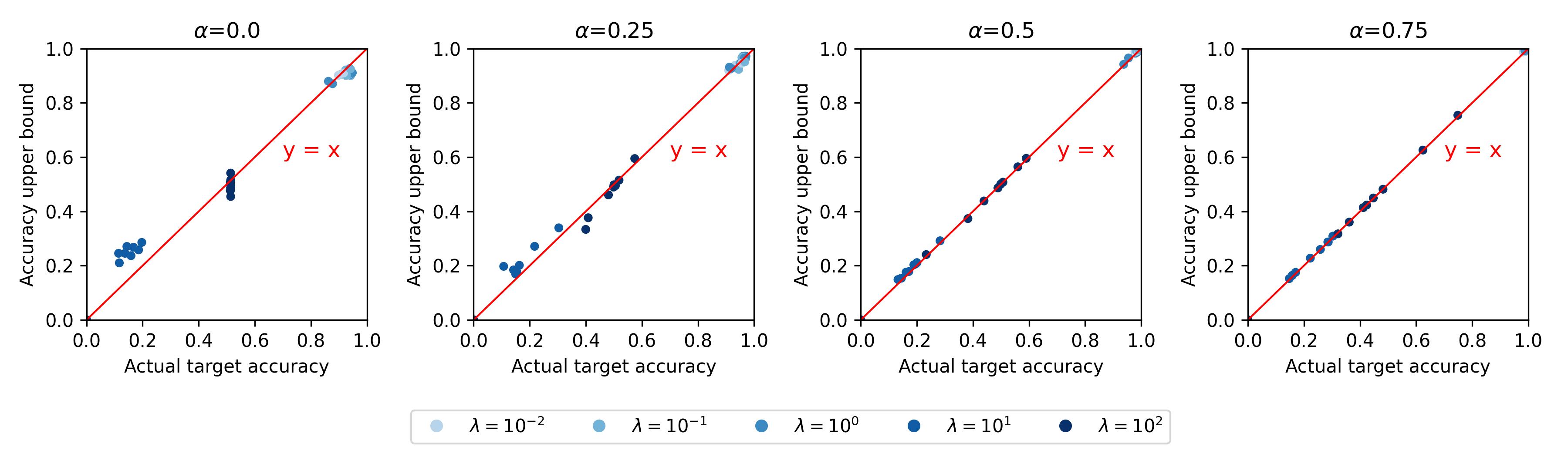
Figure 6: DIP in MNIST iii@: target accuracy upper bound obtained via Corollary 1 vs. actual target accuracy in region $\mathcal{A}$. We define region $\mathcal{A}$ as $\mathcal{A}=Q_{\alpha}\coloneqq\{X\in\mathcal{X}\mid\text{CIP predicted probability}\geq q_{\alpha}\}$, where $q_{\alpha}$ is the threshold such that $(1-\alpha)\times 100\%$ of target covariates have a CIP predicted probability greater than $q_{\alpha}$. The larger $\alpha$ is, the more confident CIP is about the prediction on the covariate samples in $Q_{\alpha}$. The red line indicates $y=x$.

5.2.2 Detecting failure of DIP in rotated MNIST

Analogous to Section 5.1.2, we apply Theorem 2 and Corollary 1 to MNIST iii@ to detect potential failures of DIP, demonstrating the second role of CICs. Figure 3 (c)(d) illustrate that the theoretical upper bound on target accuracy obtained via Theorem 2 matches closely with the actual target accuracy, and that large values of $\lambda$ such as 10 and 100 may lead DIP to learn label-flipping features, while no such issues appear in JointDIP. Figure 6 presents the result of applying Corollary 1 with different choices of region $\mathcal{A}=Q_{\alpha}$ for $\alpha\in\{0,0.25,0.5,0.75\}$. Similar to our findings in Figure 4, we observe that as CIP becomes more confident in region $\mathcal{A}$ (i.e., as $\alpha$ grows), the upper bound becomes more accurate. In Figure 7, we visualize images from the target domain sampled within the region $Q_{\alpha}$ for different values of $\alpha$. As $\alpha$ increases, the hand-written digits become more clear and distinguishable. In practice where we suspect label flipping by DIP but cannot access or afford to obtain many target labels, we can investigate target samples where CIP and DIP disagree in the region $Q_{\alpha}$ with a large value of $\alpha$, and refer to domain experts to evaluate whether these distinguishable images should be correctly classified by DIP. If DIP fails to do so, our procedure based on Corollary 1 can serve as a diagnostic tool to accurately estimate DIP’s target performance and evaluate its validity in region $\mathcal{A}$, especially when Theorem 2 provides an uninformative upper bound.

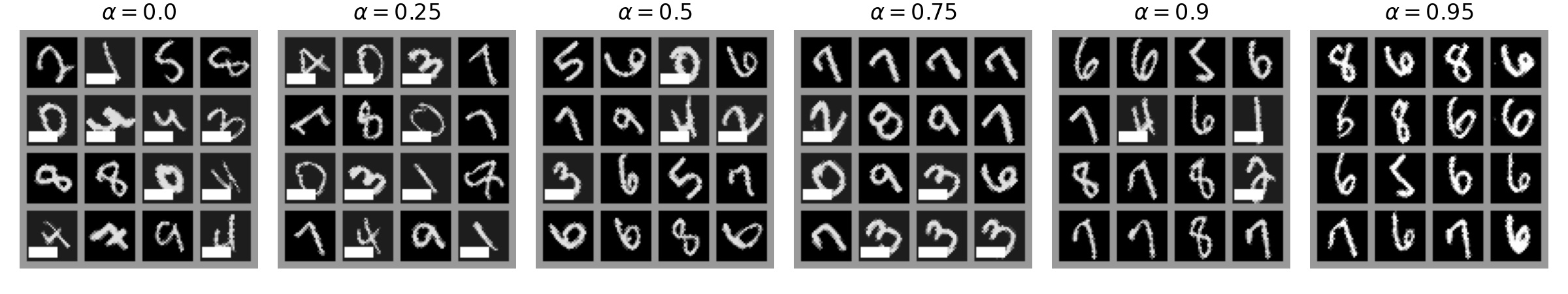
Figure 7: Sample images from MNIST iii@ target domain within region $Q_{\alpha}$ where CIP disagrees with DIP. The images are shown for varying $\alpha\in\{0,0.25,0.5,0.75,0.9,0.95\}$. As $\alpha$ increases, the selected hand-written digits become more distinguishable.

5.3 CelebA under color shift

The CelebA dataset introduced by (Liu et al., 2015) is a large-scale face image dataset with multiple face attributes. It includes over 200K celebrity images, each annotated with 40 binary attributes such as Gender, Eyeglasses, and Smiling. In our experiments, we take Smiling as the label and create six different settings for DA problems. The first three CelebA settings are designed to study the color shift together with label-flipping features, similar to the approach taken with SCM iii@ and MNIST iii@. The remaining three CelebA settings are developed to examine color shift in conjunction with label shift, similar to the approach taken with SCM ii@ and MNIST ii@. For each setting, we construct three source domains and one target domain, each consisting of 20K images randomly sampled from CelebA. The last source domain is used as the single source domain for DA algorithms that rely on a single source domain. To predict the labels, we utilize a CNN model architectures across all problem settings (see Appendix D.2 for more details).

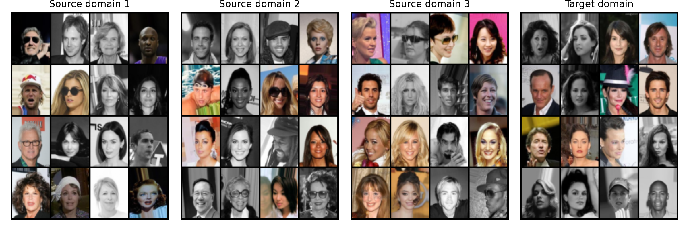
Figure 8: Sample images from CelebA iii@. In this dataset, we synthetically create a feature Color_Balance, which takes 1 for a full-color image and 0 for a black-and-white image. We also consider the original attribute Mouth_Slightly_Open, which takes 1 if the mouth in the image is slightly open, and 0 otherwise. The correlations between these two features and the label Smiling are varied across domains, as shown in Table 3.

5.3.1 Color shift with label-flipping features

The settings of CelebA i@, CelebA ii@, and CelebA iii@ are presented in Table 3. In these settings, we manipulate two features, Color_Balance and Mouth_Slightly_Open, to generate distribution shift across domains. The Color_Balance feature is a synthetic attribute, which takes a value of 1 for a full-color image and 0 for a black-and-white image. The Mouth_Slightly_Open feature is an original binary attribute annotated in the CelebA dataset, with the value 1 if the mouth in the image is slightly open, and 0 otherwise. We vary these two features so that they are conditionally independent given the label Smiling, and their correlations with this label match the values shown in Table 3. In all three settings, we align the Color_Balance feature of the last source domain and the target domain most closely, while making the correlation between Smiling and Mouth_Slightly_Open reversed. As a result, the Color_Balance feature can somewhat generalize to the target domain for label prediction, whereas the Mouth_Slightly_Open feature serves as a label-flipping feature between the last source domain and the target domain as defined in Definition 3. Figure 8 illustrates image examples from each domain in CelebA iii@. An ideal DA algorithm that utilizes the last source domain should be able to partially make use of the Color_Balance feature, but should avoid the Mouth_Slightly_Open feature to predict the labels.

	$\rho({\text{Smiling}},{\text{Color\_Balance}})$			$\rho({\text{Smiling}},{\text{Mouth\_Slightly\_Open}})$
Domain	CelebA i@	CelebA ii@	CelebA iii@	CelebA i@	CelebA ii@	CelebA iii@
Source Domain 1	-0.8	-0.8	0.2	-0.9	-0.5	-0.9
Source Domain 2	-0.6	-0.6	0.4	0.9	0.5	0.9
Source Domain 3	0.6	0.6	0.6	0.9	0.5	0.9
Target Domain	0.8	0.8	0.8	-0.9	-0.5	-0.9

Table 3: Settings of CelebA i@, ii@, iii@ under color shift with label-flipping features. Smiling is the label attribute for prediction. We vary the Color_Balance and the Mouth_Slightly_Open features across domains. The correlation between Color_Balance and Smiling remains relatively stable between the last source domain and the target domain, while Mouth_Slightly_Open serves as the label-flipping feature.

	CelebA i@		CelebA ii@		CelebA iii@
DA Algorithm	src_acc	tar_acc	src_acc	tar_acc	src_acc	tar_acc
ERM	97.0$\pm$0.2	77.7$\pm$1.2	94.4$\pm$0.4	90.3$\pm$0.9	97.0$\pm$0.2	77.7$\pm$1.2
ERM-Pool	93.3$\pm$0.3	77.2$\pm$1.4	92.8$\pm$0.4	83.6$\pm$1.0	93.1$\pm$0.2	89.6$\pm$0.4
DIP	96.2$\pm$0.4	82.0$\pm$2.2	93.1$\pm$0.3	90.6$\pm$1.0	96.2$\pm$0.4	82.0$\pm$2.2
DIP-Pool	92.3$\pm$0.5	80.4$\pm$1.3	90.9$\pm$0.4	85.5$\pm$0.6	91.6$\pm$0.3	90.4$\pm$0.4
CIP	89.1$\pm 0.3$	76.6$\pm$1.4	92.7$\pm$0.6	83.7$\pm$1.4	93.0$\pm$0.4	89.7$\pm$0.7
JointDIP	93.0$\pm$0.8	87.3$\pm$0.6	93.1$\pm$0.3	90.4$\pm$1.2	91.4$\pm$1.1	88.7$\pm$1.0
IRM	90.5$\pm$0.7	76.3$\pm$3.2	92.6$\pm$0.5	83.6$\pm$1.4	90.3$\pm$0.9	88.8$\pm$1.3
V-REx	86.9$\pm$1.2	83.3$\pm$1.2	81.8$\pm$0.2	85.1$\pm$0.7	91.8$\pm$0.3	91.1$\pm$0.8
groupDRO	91.7$\pm$1.0	84.3$\pm$1.0	91.5$\pm$0.5	86.4$\pm$1.5	92.4$\pm$0.4	91.6$\pm$0.5

Table 4: Source and target accuracy in CelebA i@, ii@, iii@ with color shift and label-flipping features. For each setting of the CelebA, DA algorithms are run on 10 different datasets, each generated using 10 different random seeds. The top four methods are highlighted in bold. The best method is colored in red.

Given that there is no label shift in these settings, we evaluate DA methods without the importance-weighted label shift correction (IW) step, and present the results in Table 4. We observe that in CelebA i@, where the correlations between Smiling and both the Color_Balance and Mouth_Slightly_Open features vary significantly across domains, JointDIP achieves the best performance. In CelebA ii@ and CelebA iii@ where we reduce the variation in correlations between Smiling and one of the features, JointDIP continues to demonstrate comparable accuracy. GroupDRO also shows a good performance, likely due to the substantial shift across domains. Overall, the results show that JointDIP maintains strong and robust performance in the presence of label-flipping features.

5.3.2 Color shift with label shift

The settings of CelebA iv@, CelebA v@, and CelebA vi@ are shown in Table 5. In these settings, we manipulate the Color_Balance feature and additionally introduce interventions on the distribution of Smiling to create label shift between the source and target domains. Speicifcally, the correlation between Smiling and the Color_Balance feature remains consistent with Table 3, but we no longer vary the Mouth_Slightly_Open feature, thereby eliminating label-flipping features between the source and target domains. Instead, we change the label distribution across domains: the distribution of Smiling is balanced (50% each) in all three source domains, but becomes unbalanced (either 75% and 25%, or 25% and 75%) in the target domain. We evaluate various DA methods, including those that incorporate the importance-weighted label shift correction (IW) step, as shown in Table 6. Given the absence of label-flipping features in these settings, we do not evaluate JointDIP. We observe that IW-DIP outperforms all other methods. Note that ERM also achieves a high accuracy and outperforms ERM-Pool, indicating that training on all source domains may not be beneficial when substantial distribution shifts, in particular the label shift, exist across domains. Overall, our experimental results highlight the importance of the label shift correction (IW) step in the presence of substantial label shift.

	$\rho({\text{Smiling}},{\text{Color\_Balance}})$			$P(\text{Smiling}=1)$
Domain	CelebA iv@	CelebA v@	CelebA vi@	CelebA iv@	CelebA v@	CelebA vi@
Source Domain 1	-0.8	-0.8	0.2	0.5	0.5	0.5
Source Domain 2	-0.6	-0.6	0.4	0.5	0.5	0.5
Source Domain 3	0.6	0.6	0.6	0.5	0.5	0.5
Target Domain	0.8	0.8	0.8	0.75	0.25	0.75

Table 5: Settings of CelebA iv@, v@, vi@ under color shift and label shift. Smiling is the label attribute for prediction. We vary the Color_Balance feature and the Smiling label distribution across domains. The correlation between Smiling and the Color_Balance feature remains consistent with Table 3. The distribution of Smiling is balanced (50% each) in all three source domains, but becomes unbalanced (either 75% and 25%, or 25% and 75%) in the target domain.

	CelebA iv@		CelebA v@		CelebA vi@
DA Algorithm	src_acc	tar_acc	src_acc	tar_acc	src_acc	tar_acc
ERM	94.4$\pm$0.6	94.1$\pm$0.5	94.4$\pm$0.6	93.9$\pm$0.9	94.5$\pm$0.6	94.2$\pm$0.5
ERM-Pool	93.6$\pm$0.2	88.7$\pm$0.9	93.6$\pm$0.2	89.6$\pm$0.9	93.8$\pm$0.3	93.1$\pm$0.5
DIP	94.4$\pm$0.4	93.5$\pm$1.2	94.4$\pm$0.5	94.4$\pm$0.9	94.4$\pm$0.4	93.4$\pm$1.2
DIP-Pool	93.7$\pm$0.6	88.0$\pm$0.6	93.6$\pm$0.5	89.5$\pm$1.2	93.7$\pm$0.5	92.9$\pm$0.9
CIP	93.4$\pm$0.4	88.3$\pm$1.0	93.4$\pm$0.4	89.7$\pm$1.1	93.6$\pm$0.2	93.3$\pm$0.5
IW-ERM	92.2$\pm$0.9	90.1$\pm$1.0	93.2$\pm$0.4	90.9$\pm$0.8	92.1$\pm$0.7	94.4$\pm$0.2
IW-CIP	91.8$\pm$0.9	90.3$\pm$0.5	92.7$\pm$1.1	90.6$\pm$1.1	91.7$\pm$1.3	94.3$\pm$0.5
IW-DIP	93.0$\pm$0.7	94.8$\pm$0.3	93.5$\pm$0.8	95.1$\pm$0.5	92.4$\pm$1.4	94.7$\pm$0.4
IRM	93.8$\pm$0.3	88.7$\pm$0.9	93.5$\pm$0.4	89.6$\pm$0.9	93.7$\pm$0.2	93.1$\pm$0.6
V-REx	92.5$\pm$0.2	89.5$\pm$0.9	92.6$\pm$0.3	90.2$\pm$1.2	93.8$\pm$0.2	93.4$\pm$0.6
groupDRO	93.3$\pm$0.3	90.0$\pm$0.8	93.3$\pm$0.3	91.1$\pm$1.0	93.7$\pm$0.3	93.0$\pm$0.6

Table 6: Source and target accuracy in CelebA iv@, v@, vi@ under color shift and label shift. For each setting of the CelebA, DA algorithms are run on 10 different datasets, each generated using 10 different random seeds. The top four methods are highlighted in bold. The best method is colored in red.

5.4 Camelyon17 from WILDS

In this subsection, we conduct numerical experiments on Camelyon17 to demonstrate the effectiveness of JointDIP on the real data. The Camelyon17 image dataset is one of the WILDS benchmarks (Koh et al., 2021; Sagawa et al., 2021) for domain adaptation, which comprises whole-slide images (WSIs) of breast cancer metastases in lymph node sections from five hospitals. The task involves predicting whether a $96\times 96$ image patch extracted from a WSI contains any tumor pixels within its central $32\times 32$ area. The labels are obtained through manual pixel-level annotations of each WSI. Among the five different hospitals (domains) from which the WSIs are collected, the first three hospitals are treated as source domains (with 302.4K patches) and the remaining two serve as validation domain (with 34.9K patches) and target domain (with 85K patches), respectively. In addition to these labeled examples, WILDS also provides additional unlabeled WSIs from the same five hospitals and patches extracted from them, including 600K unlabeled patches from the target domain. See (Koh et al., 2021; Sagawa et al., 2021) for a detailed description of the Camelyon17 dataset.

Although the 600K unlabeled target patches are collected from the same hospital as the 85K labeled target patches, there is no overlap in the WSIs where these patches are extracted from (Sagawa et al., 2021). Furthermore, the label distribution of unlabeled target patches is heavily skewed towards negative, while labeled target patches are sampled in a class-balanced manner (Sagawa et al., 2021). Consequently, this could create distribution shifts between the “unlabeled target data” and the “labeled target data” in the Camelyon17 dataset. In particular, this can lead DA algorithms, which utilize target covariate information (e.g. DIP or its variants), to identify different latent features depending on the source of target image patches used by these algorithms. In the WILDS leaderboard, methods that leverage data from the target domain utilize these 600K unlabeled patches, rather than treating the 85K labeled target patches as if they were unlabeled. However, if a distribution shift exists between the “unlabeled target data” and the “labeled target data”, there is no guarantee that our propose DA algorithms will improve target performance. Therefore, our experiments examine two approaches to utilize target data for DA methods: (1) using the 600K unlabeled target patches, and (2) leveraging the 85K labeled target patches without label access.

We use the standard DenseNet-121 model architecture (Huang et al., 2017) and follow the training protocol described in Koh et al. (2021); Sagawa et al. (2021). We implement CIP, DIP-Pool, and JointDIP-Pool, where CIP only uses labeled source data, and DIP-Pool and JointDIP-Pool leverage target covariates (image patches) from the target domain. We find that the pooled versions of DIP and JointDIP increase reliability of the models by utilizing more samples from multiple source domains, compared to their single source versions. Therefore, we choose to implement the pooled version of DIP and JointDIP in our experiments. Similarly, DANN (Ganin et al., 2016) and CORAL (Sun and Saenko, 2016), which were initially developed for the single source version, have been extended in (Sagawa et al., 2021) to take advantage of multiple source domains. Following the standard submission guidelines in WILDS (Koh et al., 2021; Sagawa et al., 2021), we do not use any data augmentation in CIP, but allow DIP-Pool and JointDIP-Pool to utilize the same color augmentation as described in Koh et al. (2021); Sagawa et al. (2021). Hyperparameters are chosen via a grid search based on the validation accuracy, where we allow a larger range of grids compared to previous experiments (see Appendix D.3 for further details).

DA Algorithm	Target covariates	val accuracy	test accuracy
IRM∗	-	86.2$\pm$1.4	64.2$\pm$8.1
groupDRO∗		85.5$\pm$2.2	68.4$\pm$7.3
ERM-Pool∗		84.9$\pm$3.1	70.3$\pm$6.4
CIP		87.0$\pm$1.2	71.1$\pm$12.5
Fish∗		83.9$\pm$1.2	74.7$\pm$7.1
DANN∗	600K unlabeled target patches	86.9$\pm$2.2	68.4$\pm$9.2
CORAL∗		90.4$\pm$0.9	77.9$\pm$6.6
DIP-Pool		91.6$\pm$0.8	81.2$\pm$8.2
JointDIP-Pool		91.5$\pm$0.6	82.7$\pm$5.2
DIP-Pool	85K labeled target patches (target labels are not used)	91.0$\pm$0.5	88.7$\pm$5.7
JointDIP-Pool		91.7$\pm$0.6	91.9$\pm$3.1

Table 7: Accuracy of DA algorithms on Camelyon17 dataset. The first five DA methods—IRM, GroupDRO, ERM-Pool, CIP, and Fish—only use labeled data from multiple source domains, whereas DANN, CORAL, DIP-Pool, and JointDIP-Pool additionally use target image patches from the target domain, but they do not have access to the target labels. The algorithms are run over 10 trials. Results for algorithms marked with ^∗ are obtained from the WILDS benchmark.

The results are presented in Table 7, where we compare CIP with other DA algorithms that enforce different invariances across all source domains, such as IRM (Arjovsky et al., 2019) and Fish (Shi et al., 2021); and we also compare DIP-Pool and JointDIP-Pool with other domain-invariant algorithms using different distributional distances, like DANN (Ganin et al., 2016) and CORAL (Sun and Saenko, 2016). We observe that CIP has a similar performance compared to ERM-Pool, albeit with a slightly larger variance in test accuracy. When covariates of 600K unlabeled target patches are utilized in the DIP matching penalty, DIP-Pool results in an accuracy exceeding $80\%$. Remarkably, JointDIP-Pool further improves this accuracy by $1.5\%$ while substantially reducing the variance at the same time. In scenarios where covariates of 85K labeled target patches are used in the DIP matching penalty, the accuracy of both methods increases significantly, with JointDIP-Pool improving DIP-Pool by over $3\%$. This result indicates that jointly matching the covariates with CICs between source and target can help DIP-based algorithms to identify the appropriate features to match across domains. In addition, when comparing the accuracy of two different approaches of using target covariates in the DIP matching penalty, our results demonstrate that distribution shifts exist between the unlabeled and labeled target data in Camelyon17, and leveraging the true target covariates from the 85K labeled target patches proves more effective than using the target covariates from the 600K unlabeled target patches.

6 Related work

As a subfield of transfer learning, domain adaptation (DA), also known as transductive transfer learning (Redko et al., 2020), aims to develop effective algorithms when distribution shifts exist across training data (source domains) and test data (target domain). In DA, it is usually assumed that we have access to some unlabeled target data, and we aim to build a model specifically for the target domain. Another related terminology domain generalization (DG), or out-of-distribution generalization (OOD) (Ben-Tal et al., 2009), instead assumes that unlabeled target data is unobtainable, and seeks a model to generalize appropriately for all possible test domains. In this paper, we do not distinguish these two terms particularly, and simply consider the DA setting, i.e., we have access to an unlabeled target dataset, and our goal is to find a classifier that performs well on the target domain.

One line of work in DA focuses on relating source and target domains by learning a common feature representation across the domains. Pan et al. (2008, 2010) first proposed to find transferable components across domains in a reproducing kernel Hilbert space, such that data distributions in different domains are close. Similar designs of creating intermediate representations across domains were investigated in (Gopalan et al., 2011; Gong et al., 2012), and later the formal idea of matching probability distributions and extracting invariant information was introduced in (Baktashmotlagh et al., 2013). They named their approach domain invariant projection (DIP), which projects data to a low-dimensional latent space where source and target covariates distributions are matched. This DIP type of approach was then widely employed in research on neural networks for DA (Sun and Saenko, 2016; Ganin et al., 2016; Hoffman et al., 2018b). Specifically, Ganin et al. (2016) first proposed to use Generative Adversarial Network (GAN) based distributional distances to learn feature representations. Since then, subsequent research has emerged that applies different neural-network-based distances (Long et al., 2017; Courty et al., 2017; Long et al., 2018; Hoffman et al., 2018b; Peng et al., 2019). While these studies have effectively demonstrated the empirical success of their methodologies across various image and text datasets, there is still a lack of understanding about the specific conditions under which these methods can achieve good target performance.

From a theoretical point of view, the rationale for DIP has been rigorously established by Ben-David et al. (2006, 2010), where they prove a target risk bound via Vapnik-Chervonenkis (VC) theory. Further studies have analyzed the source and target risk difference using different divergence measures (Mansour et al., 2009; Cortes et al., 2010; Cortes and Mohri, 2011, 2014; Hoffman et al., 2018a); see the survey by Redko et al. (2020) for a complete review. In all these works, the target risk bound typically includes three components: the source risk of the classifier, a divergence term measuring invariance of the representation, and an optimal joint error term. Then DIP objective can be viewed as minimizing the sum of the first two terms in order to achieve a low target risk. However, Johansson et al. (2019); Zhao et al. (2019) argued that DIP can completely fail in certain scenarios because the joint error term is not observable and cannot be controlled by DIP. For instance, there can be label-flipping features that achieve perfect source accuracy and invariance of representation, but result in poor performance on the target domain. Addressing how to avoid such cases in DIP has not been adequately explored.

The second class of DA methods arises from exploring invariance solely from multiple labeled source domains, without using target covariates. One such category of invariance is known as conditional invariance, which aims to discover feature representations $\phi(X)$ that are invariant conditional on the label $Y$ across source distributions. It was first introduced in Gong et al. (2016), where the authors proposed to find conditional transferable components after proper location-scale transformations. Later Heinze-Deml and Meinshausen (2017) applied a related approach by classifying features into ”core” ones, which are conditionally invariant across domains, and ”style” ones, whose distribution may shift significantly. They sought to construct a classifier built upon only the core features by imposing the conditional invariant penalty (CIP). Chen and Bühlmann (2020) further developed a theoretical framework under structural equation models to analyze the effect of CIP when the data generation process is anticausal. The emergence of conditionally invariant features, or CICs, is a natural consequence under anticausal data generation where the covariates, which are descendants of the labels, remain unperturbed. Consequently, most tasks tackled by DA methods utilizing conditional invariance typically involve anticausal problems.

It is also worth noting that under conditional invariance, it is convenient to study the label shift problem, where the marginal distributions of the label $Y$ are shifted across domains. This shift in label distribution is common in many scenarios, for example, the distribution of ArXiv paper categories can be influenced by changes in research topic trends over time (Wu et al., 2021). Lipton et al. (2018) first proposed the label shift correction algorithm, which estimates the amount of label shift by using the conditional invariance of the covariates and the moment matching equation. To ensure numerically stability, several variants of the algorithms have been further introduced. For instance, Azizzadenesheli et al. (2019) formulated an $\ell_{2}$-norm regularized least squares optimization problem, while Tachet des Combes et al. (2020) considered a constrained least squares problem and the generalized label shift assumption. Garg et al. (2020) introduced a maximum likelihood estimation approach and provided a unified view of previous label shift correction algorithms. More recently, Chen et al. (2022) has considered a distributional shift named Sparse Joint Shift (SJS), which allows for both labels and a few covariates to shift, however, the generalized label shift considered in Tachet des Combes et al. (2020) and this paper permits distribution shifts of more general latent feature representations.

Besides conditional invariance, other types of invariance have also attracted increasing attention. For example, Arjovsky et al. (2019) came up with the Invariant Risk Minimization (IRM) method to identify causal features via enforcing the invariance of label $Y$ given the features $\phi(X)$. Following IRM, analogous invariance has been explored, such as the risk invariance enforced by variance across domains (Krueger et al., 2021; Xie et al., 2020) and gradient invariance (Koyama and Yamaguchi, 2020; Shi et al., 2021). While these approaches were initially motivated to identify invariant features in causal data models, they have also been applied to anticausal problems. However, as pointed out by Rosenfeld et al. (2020); Kamath et al. (2021), IRM may fail to capture the correct invariance, especially when the model is non-linear. Counterfactual invariance is another type of invariance introduced in (Veitch et al., 2021; Jiang and Veitch, 2022), where the aim is to seek representations that are counterfactually invariant to a spurious factor of variation. (Wang and Veitch, 2022) show that the formulation of learning counterfactual invariant representations is closely related to different formulations of invariant representation learning algorithms, depending on the underlying causal structure of the data. Aside from the robustness achieved by enforcing specific invariance, a more general framework is distributionally robust optimization (DRO) (Ben-Tal et al., 2013; Duchi et al., 2016). For instance, groupDRO (Sagawa et al., 2019) intends to improve worst-group performance using an online algorithm to update group weights. It should be noted that related study of invariance and robustness has also appeared in works from a causal inference point of view (Peters et al., 2016; Meinshausen, 2018; Rothenhäusler et al., 2018; Magliacane et al., 2018).

Other DA algorithms have also been introduced based on different assumptions relating source and target data, which do not fall into the above classes of methods relying on invariance. For instance, self training, which originated from the semi-supervised learning literature (Chapelle et al., 2009), recursively adapts a classifier to fit pseudolabels predicted by a previous model using unlabeled data in a new domain (Amini and Gallinari, 2003). Theoretical properties of self training has been studied recently in (Kumar et al., 2020; Wei et al., 2020). Data augmentation serves as another beneficial way of obtaining better performance (Simard et al., 1998; Zhang et al., 2017; Yao et al., 2022), especially when possible perturbations across domains are well understood. In addition, a different perspective of DA stems from meta-learning (Thrun and Pratt, 2012; Finn et al., 2017). This “learning-to-learn” approach aims to distill knowledge of multiple learning episodes to improve future learning performance.

7 Discussion

In this paper, we highlight three prominent roles of CICs in DA. First, we propose the IW-CIP algorithm based on CICs, which can solve DA problems beyond simple covariate shift and label shift with theoretical guarantees. Specifically, we establish an explicit target risk bound for IW-CIP and further provide fine-grained analysis for each term in the bound. Second, we demonstrate the advantage of using CICs to measure the performance of other DA algorithms. For example, a conditionally invariant classifier built upon CICs can be applied as an approximate proxy for target labels to refute DA algorithms with poor target performance. Finally, to solve the label-flipping issue of DIP, we introduce the JointDIP algorithm which jointly matches the distribution of DIP features and CICs. Both our theoretical results and numerical experiments support the benefits of using CICs in DA.

While CICs across multiple source domains can be beneficial in DA, in practice it may not always be advantageous to use all available source domains for identifying CICs. Particularly, if not all source domains are related to the target domain, or if there aren’t any features invariant across all source domains, it would be more efficient to select a subset of source domains for learning CICs. However, choosing the source domains that are related to the target domain or share common features is difficult without access to target labels. In such settings, one feasible approach is to learn invariant features across possible combinations of source domains and refer to domain experts to investigate those features, which would help determine the selection of source domains. We leave the development of a framework for best source domain selection for future research.

There are other promising directions to pursue following our work. While we provide bounds in Section 4.1 to detect failure of DA algorithms, these bounds may not be tight and potentially can be improved based on other structural assumptions on the data generation model. Moreover, although in this paper we mainly focus on combing CICs with other DA algorithms, it is possible that other forms of invariance can also be applied to improve DA algorithms. For instance, can we use features obtained by IRM (Arjovsky et al., 2019), V-REx (Krueger et al., 2021), or other domain generalization algorithms to aid and enhance existing DA methods such as DIP with target risk guarantees? Finally, this paper mainly considers the unsupervised domain adaptation scenario where target labels are unavailable, however, datasets such as Camelyon17 from WILDS (Koh et al., 2021) may have a small portion of target labels available. Developing DA algorithms with target risk guarantees in such settings is therefore of practical interest.

Appendix A Illustrative examples of general anticausal model

In this section, we provide several examples for the general anticausal model and demonstrate how the conditions in Theorem 3(b) and Theorem 3(c) are satisfied under these models.

A.1 Example with CICs and label-flipping features

We present an example of the general anticausal model, as defined in Definition 4, which incorporates both CICs and label-flipping features.

Example 1

Let $Y\in\mathcal{Y}=\{1,2\}$ be a binary random variable and balanced in both domains, i.e., ${p^{{(m)}}_{1}}={p^{{(m)}}_{2}}={p^{{({\mathfrak{T}})}}_{1}}={p^{{({\mathfrak{T}})}}_{2}}=1/2$. Let $X\in{}^{3}$ be a three-dimensional covariate vector with mechanism function $f^{(1)}$ and $f^{{({\mathfrak{T}})}}$ as given by

$$f^{(1)}(1) =\begin{pmatrix}-1\\ -1\\ -1\end{pmatrix},\;f^{(1)}(2)=\begin{pmatrix}1\\ 1\\ 1\end{pmatrix};$$

$$f^{{({\mathfrak{T}})}}(1) =\begin{pmatrix}-1\\ 0\\ 1\end{pmatrix},\;f^{{({\mathfrak{T}})}}(2)=\begin{pmatrix}1\\ 2\\ -1\end{pmatrix},$$

and where the noise terms $\epsilon^{(1)}$ and $\epsilon^{{({\mathfrak{T}})}}$ are drawn from a Gaussian distribution $\mathcal{P}_{\epsilon}=\mathcal{N}(0,\mathbb{I}_{3})$. Examining each coordinate, we can see that the first coordinate ${X}_{[1]}$ maintains its conditional invariance across source and target, and thus it is a CIC. The second coordinate ${X}_{[2]}$ is perturbed, but the correlations $\rho(X^{(1)}_{[2]},Y^{(1)})=\rho(X^{{({\mathfrak{T}})}}_{[2]},Y^{{({\mathfrak{T}})}})=\sqrt{2}/2$ remian unchanged. The third coordinate ${X}_{[3]}$ is also perturbed, and by Definition 3, it is a label-flipping feature, as $\rho(X^{(1)}_{[3]},Y^{(1)})=-\rho(X^{{({\mathfrak{T}})}}_{[3]},Y^{{({\mathfrak{T}})}})=\sqrt{2}/2$.

A.2 Demonstration of condition in Theorem 3(b)

The condition (35) in Theorem 3(b) requires that for the linear conditionally invariant feature mapping $\phi_{\textnormal{inv}}$, CICs must have different conditional means for different labels. In other words, the first-moment of the CICs should suffice to distinguish between labels. We show that under the anticausal model given in the example above, this condition is indeed satisfied.

Example 1 Cont.

In Example 1, one possible linear conditionally invariant feature mapping is $\phi_{\textnormal{inv}}(x)={x}_{[1]}$, i.e., it projects to the first coordinate of the covariates. Simple algebra shows that

$$\mathbb{E}\left[{\phi_{\textnormal{inv}}(X^{(1)})}\ \middle|\ {Y^{(1)}=1}\right]=-1,\text{ and }\mathbb{E}\left[{\phi_{\textnormal{inv}}(X^{(1)})}\ \middle|\ {Y^{(1)}=2=1}\right],$$

which confirms the condition (35).

A.3 Demonstration of condition in Theorem 3(c)

While the condition (35) for linear $\phi_{\textnormal{inv}}$ is relatively straightforward, verifying the full-rank condition of matrix $C_{\phi_{\textnormal{inv}}}(a)$ for general $\phi_{\textnormal{inv}}$ in Theorem 3(c) can be more challenging due to the computation of higher-moments. Here we provide several examples where a nonlinear conditionally invariant feature mapping $\phi_{\textnormal{inv}}$ meets the full rank condition.

Example 1 Cont.

Consider the general anticausal model introduced in Example 1 ($L=2$) and let

$$\begin{split}\phi_{\textnormal{inv}}^{k}(x)&={x}_{[1]}^{k},\ \ k=0,1,2,\ldots,\text{ and }\\ \phi_{\textnormal{inv}}^{e}(x)&=\exp({x}_{[1]}).\end{split}$$ (37)

Since ${X}_{[1]}$ is a CIC, we know that $\phi_{\textnormal{inv}}^{k}({X}_{[1]})$ and $\phi_{\textnormal{inv}}^{e}({X}_{[1]})$ are also CICs. Take $a=1$ in the definition of the matrix $C_{\phi_{\textnormal{inv}}}(a)$. From the standard calculation of moments for Gaussian random variables, we have

$$C_{\phi_{\textnormal{inv}}^{k}}(a) =\begin{pmatrix}1&1\\ \mathbb{E}_{u\sim\mathcal{N}(0,1)}\left[{(u-1)^{k}}\right]&\mathbb{E}_{u\sim\mathcal{N}(0,1)}\left[{(u+1)^{k}}\right]\end{pmatrix},\;\;C_{\phi_{\textnormal{inv}}^{e}}(a)=\begin{pmatrix}1&1\\ e^{-\frac{1}{2}}&e^{\frac{3}{2}}\end{pmatrix}.$$

We conclude that $C_{\phi_{\textnormal{inv}}^{k}}(a)$ is full rank if and only if $k$ is odd, and $C_{\phi_{\textnormal{inv}}^{e}}(a)$ is a full rank matrix. Therefore, $\phi_{\textnormal{inv}}^{2k+1}(x)={x}_{[1]}^{2k+1}(k=0,1,2,\ldots)$ and $\phi_{\textnormal{inv}}^{e}(x)=\exp({x}_{[1]})$ satisfy the full rank condition.

Example 2

Consider the general anticausal model from Assumption 3 where $Y\in\mathcal{Y}=\{1,2,3\}$ with $L=3$. Let $X\in{}^{2}$ be a two-dimensional covariate vector with mechanism functions $f^{(1)}$ and $f^{{({\mathfrak{T}})}}$ defined as follows:

$$f^{(1)}(1) =\begin{pmatrix}1\\ -1\end{pmatrix},\;f^{(1)}(2)=\begin{pmatrix}2\\ 0\end{pmatrix},\ f^{(1)}(3)=\begin{pmatrix}3\\ 1\end{pmatrix};$$

$$f^{{({\mathfrak{T}})}}(1) =\begin{pmatrix}1\\ 1\end{pmatrix},\;f^{{({\mathfrak{T}})}}(2)=\begin{pmatrix}2\\ 0\end{pmatrix},\ f^{{({\mathfrak{T}})}}(3)=\begin{pmatrix}3\\ -1\end{pmatrix}.$$

That is, the first coordinate ${X}_{[1]}$ is a CIC, while the second coordinate ${X}_{[2]}$ is perturbed. Assume that the noise distribution $\mathcal{P}_{\epsilon}=\mathcal{N}(0,\mathbb{I}_{2})$ follows a Gaussian distribution. Consider the feature mappings $\phi_{\textnormal{inv}}^{2}$ and $\phi_{\textnormal{inv}}^{e}$ from Eq. (37) as the conditionally invariant feature mappings, and take $a=1$. Basic algebra shows that

$$C_{\phi_{\textnormal{inv}}^{2}}(a) =\begin{pmatrix}1&1&1\\ \mathbb{E}_{u\sim\mathcal{N}(0,1)}\left[{(u+1)^{2}}\right]&\mathbb{E}_{u\sim\mathcal{N}(0,1)}\left[{(u+2)^{2}}\right]&\mathbb{E}_{u\sim\mathcal{N}(0,1)}\left[{(u+3)^{2}}\right]\\ \mathbb{E}_{u\sim\mathcal{N}(0,1)}\left[{(u+1)^{4}}\right]&\mathbb{E}_{u\sim\mathcal{N}(0,1)}\left[{(u+2)^{4}}\right]&\mathbb{E}_{u\sim\mathcal{N}(0,1)}\left[{(u+3)^{4}}\right]\end{pmatrix}=\begin{pmatrix}1&1&1\\ 2&5&10\\ 10&43&138\end{pmatrix},$$

$$C_{\phi_{\textnormal{inv}}^{e}}(a) =\begin{pmatrix}1&1&1\\ \mathbb{E}_{u\sim\mathcal{N}(0,1)}\left[{e^{u+1}}\right]&\mathbb{E}_{u\sim\mathcal{N}(0,1)}\left[{e^{u+2}}\right]&\mathbb{E}_{u\sim\mathcal{N}(0,1)}\left[{e^{u+3}}\right]\\ \mathbb{E}_{u\sim\mathcal{N}(0,1)}\left[{e^{2(u+1)}}\right]&\mathbb{E}_{u\sim\mathcal{N}(0,1)}\left[{e^{2(u+2)}}\right]&\mathbb{E}_{u\sim\mathcal{N}(0,1)}\left[{e^{2(u+3)}}\right]\end{pmatrix}=\begin{pmatrix}1&1&1\\ e^{\frac{3}{2}}&e^{\frac{5}{2}}&e^{\frac{7}{2}}\\ e^{4}&e^{6}&e^{8}\end{pmatrix},$$

both of which are full-rank, and therefore satisfying the full rank condition in Theorem 3(c).

Example 3

Consider the general anticausal model from Assumption 3 with arbitrary number of classes $L\geq 2$. Let

$$f^{(m)}(y)=\begin{pmatrix}e_{y}\\ a_{y}^{(m)}\end{pmatrix},f^{{({\mathfrak{T}})}}(y)=\begin{pmatrix}e_{y}\\ a_{y}^{{({\mathfrak{T}})}}\end{pmatrix},$$

where $e_{i}\in{}^{L}$ denotes the zero vector with only the $i$-th element being $1$, and $a_{y}^{(m)},a_{y}^{{({\mathfrak{T}})}}\in{}^{p-L}$ $(p>L)$ are arbitrary vectors. That is, the first $L$ covariates are CICs while the last $p-L$ coordinates can be arbitrarily perturbed. Let

$$\phi_{\textnormal{inv}}^{k}(X)=\begin{pmatrix}{X}_{[1]}^{k},{X}_{[2]}^{k},\cdots,{X}_{[L]}^{k}\end{pmatrix}^{\top},\ \ k=1,2,\ldots.$$

For a fixed vector $a\in{}^{L}$, verifying $C_{\phi_{\textnormal{inv}}^{k}}(a)$ is full rank can be technical depending on the distribution $\mathcal{P}_{\epsilon}$. Instead, we show an illustrative explanation rather than a rigorous proof. First, let’s consider $\mathcal{P}_{\epsilon}=\delta_{0}(\cdot)$, the Dirac distribution centered at 0. Then we can compute

$$C_{\phi_{\textnormal{inv}}^{k}}(a)=\begin{pmatrix}1&1&\cdots&1\\ {a}_{[1]}&{a}_{[2]}&\cdots&{a}_{[L]}\\ \vdots&\vdots&\ddots&\vdots\\ {a}_{[1]}^{L-1}&{a}_{[2]}^{L-1}&\cdots&{a}_{[L]}^{L-1}\end{pmatrix},$$

which is a Vandermonde matrix and is full rank as long as we take ${a}_{[i]}\neq{a}_{[j]},i\neq j$. Next we consider a case where $\mathcal{P}_{\epsilon}$ is a distribution concentrated around 0 (e.g. a Gaussian distribution with very small variance). In this case, the matrix will be slightly perturbed but is still full rank by the continuity of high-order moments and matrix determinants.

Appendix B Proof of Section 3 and additional results on IW-CIP

In this section we prove our main theorems and propositions given in Section 3, as well as additional results given in Proposition 5 and Lemma 1. Proposition 5 provides the finite-sample bound for the IW-CIP penalty when it is defined by the squared mean distance, and Lemma 1 proves the number of required source domains to validate the conditions in Proposition 3 when the perturbations are randomly generated.

B.1 Proof of Theorem 1.A

Let $w=(w^{(1)},\ldots,w^{(M)})$ where $w^{(m)}$ is the true importance weight for the $m$-th source domain. For any classifier $h=g\circ\phi$, we have

$$\mathcal{R}^{{({\mathfrak{T}})}}({h})-\overline{\mathcal{R}}({h};{w})$$

$$={\frac{1}{M}}\sum_{m=1}^{M}\left(\mathbb{E}\left[{\mathbf{1}_{{h(X^{{({\mathfrak{T}})}})\neq Y^{{({\mathfrak{T}})}}}}}\right]-\mathbb{E}\left[{{w}_{[Y^{(m)}]}^{(m)}\cdot\mathbf{1}_{{h(X^{(m)})\neq Y^{(m)}}}}\right]\right)$$

$$={\frac{1}{M}}\sum_{m=1}^{M}\sum_{y=1}^{L}\left(\mathbb{P}\left\{{h(X^{{({\mathfrak{T}})}})\neq y}\ \middle|\ {Y^{{({\mathfrak{T}})}}=y}\right\}-\mathbb{P}\left\{{h(X^{(m)})\neq y}\ \middle|\ {Y^{(m)}=y}\right\}\right)\mathbb{P}\left\{{Y^{{({\mathfrak{T}})}}=y}\right\}$$

$$={\frac{1}{M}}\sum_{m=1}^{M}\sum_{y=1}^{L}\left(\mathbb{P}\left\{{h(X^{{({\mathfrak{T}})}})=y}\ \middle|\ {Y^{{({\mathfrak{T}})}}=y}\right\}-\mathbb{P}\left\{{h(X^{(m)})=y}\ \middle|\ {Y^{(m)}=y}\right\}\right)\mathbb{P}\left\{{Y^{{({\mathfrak{T}})}}=y}\right\},$$

where the second step applies ${w}_{[y]}^{(m)}=\frac{\mathbb{P}\left\{{Y^{{({\mathfrak{T}})}}=y}\right\}}{\mathbb{P}\left\{{Y^{(m)}=y}\right\}}$ and the law of total expectation. By definition of $D_{\mathcal{G}}\left({\cdot},{\cdot}\right)$, it is then upper bounded by

$$\left|\mathcal{R}^{{({\mathfrak{T}})}}({h})-\overline{\mathcal{R}}({h};{w})\right| \leq{\frac{1}{M}}\sum_{m=1}^{M}\sum_{y=1}^{L}D_{\mathcal{G}}\left({\mathcal{P}^{{({\mathfrak{T}})}}_{{\phi(X)}|{Y=y}}},{\mathcal{P}^{(m)}_{{\phi(X)}|{Y=y}}}\right)\mathbb{P}\left\{{Y^{{({\mathfrak{T}})}}=y}\right\}$$

$$\leq\max_{\begin{subarray}{c}m=1,\ldots,M,\\ y=1,\ldots,L\end{subarray}}D_{\mathcal{G}}\left({\mathcal{P}^{{({\mathfrak{T}})}}_{{\phi(X)}|{Y=y}}},{\mathcal{P}^{(m)}_{{\phi(X)}|{Y=y}}}\right)\sum_{m=1}^{M}{\frac{1}{M}}\sum_{y=1}^{L}\mathbb{P}\left\{{Y^{{({\mathfrak{T}})}}=y}\right\}$$

$$=\max_{\begin{subarray}{c}m=1,\ldots,M,\\ y=1,\ldots,L\end{subarray}}D_{\mathcal{G}}\left({\mathcal{P}^{{({\mathfrak{T}})}}_{{\phi(X)}|{Y=y}}},{\mathcal{P}^{(m)}_{{\phi(X)}|{Y=y}}}\right)$$

$$=\Psi_{\mathcal{G},\phi},$$ (38)

where we use $\sum_{y=1}^{L}\mathbb{P}\left\{{Y^{{({\mathfrak{T}})}}=y}\right\}=1$ and $\sum_{m=1}^{M}1/M=1$ in the second step. Furthermore, we can bound

$$\left|\mathcal{R}^{(m)}({h};{w^{(m)}})-\mathcal{R}^{(m)}({h};{\widehat{w}^{(m)}})\right| =\left|\mathbb{E}\left[{\left({w}_{[Y^{(m)}]}^{(m)}-{\widehat{w}}_{[Y^{(m)}]}^{(m)}\right)\cdot\mathbf{1}_{{h(X^{(m)})\neq Y^{(m)}}}}\right]\right|$$

$$\leq\lVert{w^{(m)}-\widehat{w}^{(m)}}\rVert_{\infty}.$$

It follows that

$$\left|\overline{\mathcal{R}}({h};{w})-\overline{\mathcal{R}}({h};{\widehat{w}})\right| \leq{\frac{1}{M}}\sum_{m=1}^{M}\left|\mathcal{R}^{(m)}({h};{w^{(m)}})-\mathcal{R}^{(m)}({h};{\widehat{w}^{(m)}})\right|$$

$$\leq\max_{m=1,\ldots,M}\lVert{w^{(m)}-\widehat{w}^{(m)}}\rVert_{\infty}.$$ (39)

The result now follows from combining Eq. (B.1) and Eq. (B.1).

B.2 Proof of Theorem 1.B

Denote the empirical average source risk across $M$ environments by

$$\widehat{\overline{\mathcal{R}}}({h};{{\rm w}^{(m)}})=\frac{1}{M}\sum_{m=1}^{M}\widehat{\mathcal{R}}^{(m)}({h};{{\rm w}^{(m)}}).$$

Then we can write

$$\quad\mathcal{R}^{{({\mathfrak{T}})}}({\widehat{h}_{\textnormal{IW-CIP}}})-\mathcal{R}^{{({\mathfrak{T}})}}({h^{\star}})$$

$$=\underbrace{\mathcal{R}^{{({\mathfrak{T}})}}({\widehat{h}_{\textnormal{IW-CIP}}})-\overline{\mathcal{R}}({\widehat{h}_{\textnormal{IW-CIP}}};{w})}_{(A_{1})}+\underbrace{\overline{\mathcal{R}}({\widehat{h}_{\textnormal{IW-CIP}}};{w})-\widehat{\overline{\mathcal{R}}}({\widehat{h}_{\textnormal{IW-CIP}}};{w})}_{(B_{1})}+$$

$$\quad+\underbrace{\widehat{\overline{\mathcal{R}}}({\widehat{h}_{\textnormal{IW-CIP}}};{w})-\widehat{\overline{\mathcal{R}}}({\widehat{h}_{\textnormal{IW-CIP}}};{\widehat{w}})}_{(C_{1})}+\underbrace{\widehat{\overline{\mathcal{R}}}({\widehat{h}_{\textnormal{IW-CIP}}};{\widehat{w}})-\widehat{\overline{\mathcal{R}}}({h^{\star}};{\widehat{w}})}_{(D)}+\underbrace{\widehat{\overline{\mathcal{R}}}({h^{\star}};{\widehat{w}})-\widehat{\overline{\mathcal{R}}}({h^{\star}};{w})}_{(C_{2})}$$

$$\quad+\underbrace{\widehat{\overline{\mathcal{R}}}({h^{\star}};{w})-\overline{\mathcal{R}}({h^{\star}};{w})}_{(B_{2})}+\underbrace{\overline{\mathcal{R}}({h^{\star}};{w})-\mathcal{R}^{{({\mathfrak{T}})}}({h^{\star}})}_{(A_{2})}.$$

Term $A_{1}$ and $A_{2}$

From Eq. (B.1) in the proof of Theorem 1.A, we have

$$\begin{split}A_{1}&=\mathcal{R}^{{({\mathfrak{T}})}}({\widehat{h}_{\textnormal{IW-CIP}}})-\overline{\mathcal{R}}({\widehat{h}_{\textnormal{IW-CIP}}};{w})\leq\Psi_{\mathcal{G},\widehat{\phi}_{\textnormal{IW-CIP}}},\\ A_{2}&=\overline{\mathcal{R}}({h^{\star}};{w})-\mathcal{R}^{{({\mathfrak{T}})}}({h^{\star}})=0.\end{split}$$ (40)

The second equation follows from the definition of $h^{\star}=g^{\star}\circ\phi^{\star}$, i.e., $\phi^{\star}$ is a conditionally invariant feature mapping and satisfies $\Psi_{\mathcal{G},\phi^{\star}}=0$.

Term $B_{1}$ and $B_{2}$

For any $h=g\circ\phi$, we have $\left|{w}_{[Y^{(m)}]}^{(m)}\mathbf{1}_{{h(X^{(m)})\neq Y^{(m)}}}\right|\leq\left\|w^{(m)}\right\|_{\infty}$. Then the generalization bound based on Rademacher complexity (see e.g. (Wainwright, 2019, Theorem 4.10)) shows that, for the $m$-th source domain, the bound

$$\sup_{\begin{subarray}{c}h=g\circ\phi\\ g\in\mathcal{G},\phi\in\Phi\end{subarray}}\left|\mathcal{R}^{(m)}({h};{w^{(m)}})-\widehat{\mathcal{R}}^{(m)}({h};{w^{(m)}})\right| \leq 2\mathfrak{R}_{n^{(m)},\mathcal{P}^{(m)}}\left({\mathcal{H}(w^{(m)},\mathcal{G},\Phi)}\right)$$

$$\hskip 50.00008pt+\left\|w^{(m)}\right\|_{\infty}\sqrt{\frac{2\log(M/\delta)}{n^{(m)}}},$$

holds with probability at least $1-\delta/M$. Using the union bound over each $m\in\{1,\ldots,M\}$, we obtain that with probability at least $1-\delta$,

$$\left|B_{1}\right|+\left|B_{2}\right| \leq 2\sup_{\begin{subarray}{c}h=g\circ\phi,\\ g\in\mathcal{G},\phi\in\Phi\end{subarray}}{\frac{1}{M}}\sum_{m=1}^{M}\left|\mathcal{R}^{(m)}({h};{w^{(m)}})-\widehat{\mathcal{R}}^{(m)}({h};{w^{(m)}})\right|$$

$$\leq\max_{m=1,\ldots,M}\left[4\mathfrak{R}_{n^{(m)},\mathcal{P}^{(m)}}\left({\mathcal{H}(w^{(m)},\mathcal{G},\Phi)}\right)+2\left\|w^{(m)}\right\|_{\infty}\sqrt{\frac{2\log(M/\delta)}{n^{(m)}}}\right].$$ (41)

Term $C_{1}$ and $C_{2}$

For the $m$-th source domain, let us define

$$\widehat{\ell}^{(m)}_{j}=\sum_{k=1}^{n}\mathbf{1}_{{Y^{(m)}_{k}=j}}\mathbf{1}_{{h(X^{(m)}_{k})\neq Y^{(m)}_{k}}}.$$

Then $\lVert{\widehat{\ell}^{(m)}}\rVert_{1}\leq n$ and so for any $h=g\circ\phi$,

$$\left|\widehat{\mathcal{R}}^{(m)}({h};{w^{(m)}})-\widehat{\mathcal{R}}^{(m)}({h};{\widehat{w}^{(m)}})\right| =\left|\frac{1}{n}\sum_{k=1}^{n}\left({w}_{[Y^{(m)}_{k}]}^{(m)}-{\widehat{w}}_{[Y^{(m)}_{k}]}^{(m)}\right)\mathbf{1}_{{h(X^{(m)}_{k})\neq Y^{(m)}_{k}}}\right|$$

$$=\left|\frac{1}{n}\sum_{j=1}^{L}\left({w}_{[j]}^{(m)}-{\widehat{w}}_{[j]}^{(m)}\right)\widehat{\ell}^{(m)}_{j}\right|$$

$$\leq\frac{1}{n}\left\|w^{(m)}-\widehat{w}^{(m)}\right\|_{\infty}\left\|\widehat{\ell}^{(m)}\right\|_{1}\leq\left\|w^{(m)}-\widehat{w}^{(m)}\right\|_{\infty}.$$

It follows that

$$\left|C_{1}\right|+\left|C_{2}\right| \leq 2\sup_{\begin{subarray}{c}h=g\circ\phi,\\ g\in\mathcal{G},\phi\in\Phi\end{subarray}}{\frac{1}{M}}\sum_{m=1}^{M}\left|\widehat{\mathcal{R}}^{(m)}({h};{w^{(m)}})-\widehat{\mathcal{R}}^{(m)}({h};{\widehat{w}^{(m)}})\right|$$

$$\leq 2\max_{m=1,\ldots,M}\left\|w^{(m)}-\widehat{w}^{(m)}\right\|_{\infty}.$$ (42)

Term $D$

By definition of $\widehat{h}_{\textnormal{IW-CIP}}$ from Eq. (3.2), we know that

$$\widehat{\overline{\mathcal{R}}}({\widehat{h}_{\textnormal{IW-CIP}}};{\widehat{w}})+\widehat{\Lambda}_{\widehat{\phi}_{\textnormal{IW-CIP}}}\leq\widehat{\overline{\mathcal{R}}}({h^{\star}};{\widehat{w}})+\widehat{\Lambda}_{\phi^{\star}},$$

and so rearranging terms,

$$D=\widehat{\overline{\mathcal{R}}}({\widehat{h}_{\textnormal{IW-CIP}}};{\widehat{w}})-\widehat{\overline{\mathcal{R}}}({h^{\star}};{\widehat{w}})\leq\widehat{\Lambda}_{\phi^{\star}}-\widehat{\Lambda}_{\widehat{\phi}_{\textnormal{IW-CIP}}}\leq\widehat{\Lambda}_{\phi^{\star}}.$$ (43)

The theorem then follows from combining Eq. (40), (B.2), (B.2), and (43).

B.3 Proof of Proposition 1

For a family of functions $\mathcal{G}$ mapping $\mathcal{Z}$ to $[0,1]$ and a distribution $\mathcal{P}$ on $\mathcal{Z}$, let $\widehat{\mathcal{P}}_{n}$ denote the empirical distribution of $n$ $i.i.d.$ samples $(Z_{1},Z_{2},\ldots,Z_{n})$ from $\mathcal{P}$. The standard Rademacher complexity theory (see e.g. (Wainwright, 2019, Theorem 4.10)) states that for any $\delta>0$, with probability at least $1-\delta$, we have

$$\sup_{g\in\mathcal{G}}\left|\mathbb{E}_{Z\sim\mathcal{P}}\left[{g(Z)}\right]-\mathbb{E}_{Z\sim\widehat{\mathcal{P}}_{n}}\left[{g(Z)}\right]\right|\leq 2\mathfrak{R}_{n,\mathcal{P}}\left({\mathcal{G}}\right)+\sqrt{\frac{\log(2/\delta)}{2n}}.$$

By definition of $\mathcal{G}$-divergence, with probability $1-\delta$ we have

$$D_{\mathcal{G}}\left({\mathcal{P}},{\widehat{\mathcal{P}}_{n}}\right) =\sup_{g\in\mathcal{G}}\max_{y=1,2,\ldots,L}\left|\mathbb{E}_{Z\sim\mathcal{P}}\left[{\mathbf{1}_{{g(Z)=y}}}\right]-\mathbb{E}_{Z\sim\widehat{\mathcal{P}}_{n}}\left[{\mathbf{1}_{{g(Z)=y}}}\right]\right|$$

$$=\max_{y=1,2,\ldots,L}\sup_{g\in\mathcal{G}}\left|\mathbb{E}_{Z\sim\mathcal{P}}\left[{\mathbf{1}_{{g(Z)=y}}}\right]-\mathbb{E}_{Z\sim\widehat{\mathcal{P}}_{n}}\left[{\mathbf{1}_{{g(Z)=y}}}\right]\right|$$

$$\leq\max_{y=1,2,\ldots,L}\left(2\mathfrak{R}_{n,\mathcal{P}}\left({\mathcal{G}_{y}}\right)+\sqrt{\frac{\log(2L/\delta)}{2n}}\right),$$ (44)

where $\mathcal{G}_{y}\coloneqq\left\{\mathbf{1}_{{g(x)=y}},g\in\mathcal{G}\right\}$. Then we can bound

$$\quad D_{\mathcal{G}}\left({\widehat{\mathcal{P}}^{(m)}_{{\phi^{\star}(X)}|{Y=y}}},{\widehat{\mathcal{P}}^{(m^{\prime})}_{{\phi^{\star}(X)}|{Y=y}}}\right)$$

$$\overset{(i)}{\leq}D_{\mathcal{G}}\left({\widehat{\mathcal{P}}^{(m)}_{{\phi^{\star}(X)}|{Y=y}}},{\mathcal{P}^{(m)}_{{\phi^{\star}(X)}|{Y=y}}}\right)+D_{\mathcal{G}}\left({\mathcal{P}^{(m)}_{{\phi^{\star}(X)}|{Y=y}}},{\mathcal{P}^{(m^{\prime})}_{{\phi^{\star}(X)}|{Y=y}}}\right)$$

$$\hskip 30.00005pt+D_{\mathcal{G}}\left({\mathcal{P}^{(m^{\prime})}_{{\phi^{\star}(X)}|{Y=y}}},{\widehat{\mathcal{P}}^{(m^{\prime})}_{{\phi^{\star}(X)}|{Y=y}}}\right)$$

$$\overset{(ii)}{=}D_{\mathcal{G}}\left({\widehat{\mathcal{P}}^{(m)}_{{\phi^{\star}(X)}|{Y=y}}},{\mathcal{P}^{(m)}_{{\phi^{\star}(X)}|{Y=y}}}\right)+D_{\mathcal{G}}\left({\widehat{\mathcal{P}}^{(m^{\prime})}_{{\phi^{\star}(X)}|{Y=y}}},{\mathcal{P}^{(m^{\prime})}_{{\phi^{\star}(X)}|{Y=y}}}\right),$$ (45)

where in step $(i)$ we apply triangular inequality, and in step $(ii)$ we use the fact that $\phi^{\star}$ is a conditionally invariant feature mapping across source domains to cancel the middle term. Applying union bound, we get

$$\widehat{\Lambda}_{\phi^{\star}} =\frac{\lambda_{\textnormal{IW-CIP}}}{LM^{2}}\sum_{y=1}^{L}\sum_{m\neq m^{\prime}}D_{\mathcal{G}}\left({\widehat{\mathcal{P}}^{(m)}_{{\phi^{\star}(X)}|{Y=y}}},{\widehat{\mathcal{P}}^{(m^{\prime})}_{{\phi^{\star}(X)}|{Y=y}}}\right)$$

$$\overset{(i)}{\leq}\frac{2\lambda_{\textnormal{IW-CIP}}}{LM}\sum_{y=1}^{L}\sum_{m=1}^{M}D_{\mathcal{G}}\left({\mathcal{P}^{(m)}_{{\phi^{\star}(X)}|{Y=y}}},{\widehat{\mathcal{P}}^{(m)}_{{\phi^{\star}(X)}|{Y=y}}}\right)$$

$$\overset{(ii)}{\leq}\frac{4\lambda_{\textnormal{IW-CIP}}}{LM}\cdot\sum_{y=1}^{L}\sum_{m=1}^{M}\max_{y^{\prime}=1,2,\ldots,L}\mathfrak{R}_{n^{(m)},\mathcal{P}^{(m)}_{{\phi^{\star}(X)}|{Y=y}}}\left({\mathcal{G}_{y^{\prime}}}\right)+\frac{2\lambda_{\textnormal{IW-CIP}}}{M}\sum_{m=1}^{M}\sqrt{\frac{\log(2LM/\delta)}{2n^{(m)}}}$$

$$\leq 2\lambda_{\textnormal{IW-CIP}}\left(2\max_{\begin{subarray}{c}m=1,2,\ldots,M\\ y=1,2,\ldots,L\\ y^{\prime}=1,2,\ldots,L\end{subarray}}\mathfrak{R}_{n^{(m)},\mathcal{P}^{(m)}_{{\phi^{\star}(X)}|{Y=y}}}\left({\mathcal{G}_{y^{\prime}}}\right)+\max_{m=1,2,\ldots,M}\sqrt{\frac{\log(2LM/\delta)}{2n^{(m)}}}\right),$$

with probability at least $1-\delta$. Here step $(i)$ uses Eq. (B.3) and step $(ii)$ uses Eq. (B.3). This completes the proof of the proposition.

B.4 Another bound on $\widehat{\Lambda}_{\phi^{\star}}$ under mean squared distance

In Proposition 1 we established a finite-sample bound for $\widehat{\Lambda}_{\phi^{\star}}$ when $\mathcal{G}$-divergence is used. If the IW-CIP penalty is defined by the squared mean distance instead, we provide another explicit bound for $\widehat{\Lambda}_{\phi^{\star}}$ that converges to zero as sample size goes to infinity. To show this, we require additional assumptions on the data generation model and the class of feature mappings $\Phi$.

Proposition 5

Suppose that source and target data are generated under Assumption 1. Let $\Phi=\{\phi(x)=Ax+b,A\in{}^{q\times p},b\in{}^{q}\}$ be the linear class of feature mappings from ^p to ^q $(q\leq p)$, and let the squared mean distance be the distributional distance in IW-CIP penalty Eq. (19). Suppose $\phi\in\Phi$ is a conditionally invariant feature mapping such that $A\Sigma A^{\top}$ is non-singular. For any $\delta>0$ satisfying $\min_{m,y}n^{(m)}{p^{{(m)}}_{y}}\geq 2\log(2ML/\delta)$, we have

$$\widehat{\Lambda}_{\phi} \leq\frac{12\lambda_{\textnormal{IW-CIP}}\cdot\lambda_{\rm max}(A\Sigma{A}^{\top})\cdot\left(p+8\log(2ML/\delta)\right)}{\underset{\begin{subarray}{c}m=1,2,\ldots,M\\ y=1,2,\ldots,L\end{subarray}}{\min}\ n^{(m)}{p^{{(m)}}_{y}}-2\log(2ML/\delta)},$$ (46)

with probability at least $1-\delta$. Specifically, the statement holds for the optimal conditionally invariant mapping $\phi^{\star}$ (see Eq. (5)).

Proof  The exact from of IW-CIP penalty under squared mean distance is

$$\widehat{\Lambda}_{\phi} \coloneqq\frac{\lambda_{\textnormal{IW-CIP}}}{LM^{2}}\sum_{y=1}^{L}\sum_{m\neq m^{\prime}}\Bigg{\|}\widehat{\mu^{(m)}_{\phi}(y)}-\widehat{\mu^{(m^{\prime})}_{\phi}(y)}\Bigg{\|}_{2}^{2},$$

where

$$\widehat{\mu^{(m)}_{\phi}(y)}=\frac{1}{n^{(m)}_{y}}\sum_{\begin{subarray}{c}k=1\\ Y^{(m)}_{k}=y\end{subarray}}^{n^{(m)}}\phi(X^{(m)}_{k}),$$

is the empirical mean of $\phi(X)$ on the $m$-th source domain. Since $\phi$ is conditionally invariant, from Eq. (52) we know that for any $y\in\left\{1,2,\ldots,L\right\}$ and for any $m\neq m^{\prime}$,

$$A{P_{y}}{v^{{(m)}}_{y}}=A{P_{y}}{v^{{(m^{\prime})}}_{y}}.$$

In the finite-sample case, when $Y^{(m)}_{k}=Y^{{({\mathfrak{T}})}}_{k}=y$, we can write

$$\phi(X^{(m)}_{k})=AX^{(m)}_{k}+b =A\left(f^{(1)}(y)+{P_{y}}{v^{{(m)}}_{y}}+\epsilon^{{(m)}}_{k}\right)+b,$$

$$\phi(X^{{({\mathfrak{T}})}}_{k})=AX^{{({\mathfrak{T}})}}_{k}+b =A\left(f^{(1)}(y)+{P_{y}}{v^{{({\mathfrak{T}})}}_{y}}+\epsilon^{{({\mathfrak{T}})}}_{k}\right)+b,$$

and

$$\widehat{\mu^{(m)}_{\phi}(y)}-\widehat{\mu^{(m^{\prime})}_{\phi}(y)} =\frac{1}{n^{(m)}_{y}}\sum_{\begin{subarray}{c}k=1\\ Y^{(m)}_{k}=y\end{subarray}}^{n^{(m)}}\phi(X^{(m)}_{k})-\frac{1}{n^{(m^{\prime})}_{y}}\sum_{\begin{subarray}{c}k=1\\ Y^{(m^{\prime})}_{k}=y\end{subarray}}^{n^{(m^{\prime})}}\phi(X^{(m^{\prime})}_{k})$$

$$=A\left(\underbrace{\frac{1}{n^{(m)}_{y}}\sum_{\begin{subarray}{c}k=1\\ Y^{(m)}_{k}=y\end{subarray}}^{n^{(m)}}\epsilon^{{(m)}}_{k}}_{e^{(m)}_{y}}-\underbrace{\frac{1}{n^{(m^{\prime})}_{y}}\sum_{\begin{subarray}{c}k=1\\ Y^{(m^{\prime})}_{k}=y\end{subarray}}^{n^{(m^{\prime})}}\epsilon^{(m^{\prime})}_{k}}_{e_{y}^{(m^{\prime})}}\right),$$ (47)

where $n^{(m)}_{y}$ is the number of samples with label $y$ in the $m$-th domain. Since $n_{y}^{(m)}$ follows a multinomial distribution, we conclude from binomial (multinomial) tail probability bound (e.g. (Chung and Lu, 2006, Theorem 3.2)) that for all ${t_{y}^{(m)}}>0$,

$$\mathbb{P}\left\{{n^{(m)}_{y}\geq n^{(m)}{p^{{(m)}}_{y}}(1-{t_{y}^{(m)}})}\right\} \geq 1-\exp\left(-\frac{n^{(m)}{p^{{(m)}}_{y}}{t_{y}^{(m)}}^{2}}{2}\right).$$

When $n^{(m)}_{y}=k>0$ is fixed, we have $Ae^{(m)}_{y}\sim\mathcal{N}(0,\frac{1}{k}A\Sigma A^{\top})$, and therefore the standard concentration bound for Gaussian variables (e.g. (Wainwright, 2019, Example 2.11)) implies that for all $t>0$,

$$\mathbb{P}\left\{{\left\|Ae^{(m)}_{y}\right\|_{2}^{2}\leq\frac{1}{k}\lambda_{\rm max}\left(A\Sigma A^{\top}\right)\cdot p\left(1+t\right)}\ \middle|\ {n^{(m)}_{y}=k}\right\}\geq 1-e^{-p\min\{t,t^{2}\}/8}.$$

Next we combine two bounds above into a single bound for $\left\|Ae^{(m)}_{y}\right\|_{2}^{2}$. Given any $t_{y}^{(m)}>0$ and $t>0$, we have

$$\quad\mathbb{P}\left\{{\left\|Ae^{(m)}_{y}\right\|_{2}^{2}\leq\frac{\lambda_{\rm max}\left(A\Sigma A^{\top}\right)\cdot p\left(1+t\right)}{n^{(m)}{p^{{(m)}}_{y}}(1-{t_{y}^{(m)}})}}\right\}$$

$$=\sum_{k=0}^{n^{(m)}}\mathbb{P}\left\{{\left\|Ae^{(m)}_{y}\right\|_{2}^{2}\leq\frac{\lambda_{\rm max}\left(A\Sigma A^{\top}\right)\cdot p\left(1+t\right)}{n^{(m)}{p^{{(m)}}_{y}}(1-{t_{y}^{(m)}})}}\ \middle|\ {n^{(m)}_{y}=k}\right\}\mathbb{P}\left\{{n^{(m)}_{y}=k}\right\}$$

$$\geq\sum_{k=n^{(m)}{p^{{(m)}}_{y}}(1-{t_{y}^{(m)}})}^{n^{(m)}}\mathbb{P}\left\{{\left\|Ae^{(m)}_{y}\right\|_{2}^{2}\leq\frac{\lambda_{\rm max}\left(A\Sigma A^{\top}\right)\cdot p\left(1+t\right)}{n^{(m)}{p^{{(m)}}_{y}}(1-{t_{y}^{(m)}})}}\ \middle|\ {n^{(m)}_{y}=k}\right\}\mathbb{P}\left\{{n^{(m)}_{y}=k}\right\}$$

$$\geq\sum_{k=n^{(m)}{p^{{(m)}}_{y}}(1-{t_{y}^{(m)}})}^{n^{(m)}}\mathbb{P}\left\{{\left\|Ae^{(m)}_{y}\right\|_{2}^{2}\leq\frac{1}{k}\lambda_{\rm max}\left(A\Sigma A^{\top}\right)\cdot p\left(1+t\right)}\ \middle|\ {n^{(m)}_{y}=k}\right\}\mathbb{P}\left\{{n^{(m)}_{y}=k}\right\}$$

$$\geq\sum_{k=n^{(m)}{p^{{(m)}}_{y}}(1-{t_{y}^{(m)}})}^{n^{(m)}}\left(1-e^{-p\min\{t,t^{2}\}/8}\right)\mathbb{P}\left\{{n^{(m)}_{y}=k}\right\}$$

$$\geq\left(1-e^{-p\min\{t,t^{2}\}/8}\right)\left(1-e^{-{n^{(m)}{p^{{(m)}}_{y}}{t_{y}^{(m)}}^{2}}/{2}}\right)$$

$$\geq 1-e^{-p\min\{t,t^{2}\}/8}-e^{-{n^{(m)}{p^{{(m)}}_{y}}{t_{y}^{(m)}}^{2}}/{2}}.$$

Take ${t_{y}^{(m)}}=\sqrt{2\log(2ML/\delta)/(n^{(m)}{p^{{(m)}}_{y}})}$ and $t=8\log(2ML/\delta)/p+\sqrt{8\log(2ML/\delta)/p}$. Then with probability at least $1-\delta/ML$, we have

$$\left\|Ae^{(m)}_{y}\right\|_{2}^{2} \leq\frac{\lambda_{\rm max}\left(A\Sigma A^{\top}\right)\left(p+8\log(2ML/\delta)+\sqrt{8p\log(2ML/\delta)}\right)}{n^{(m)}{p^{{(m)}}_{y}}-\sqrt{n^{(m)}{p^{{(m)}}_{y}}\cdot 2\log\left(2ML/\delta\right)}}$$

$$\leq\frac{3\lambda_{\rm max}\left(A\Sigma A^{\top}\right)\left(p+8\log(2ML/\delta)\right)}{n^{(m)}{p^{{(m)}}_{y}}-2\log(2ML/\delta)},$$

where we apply the inequality $\sqrt{ab}\leq(a+b)/2$ for $a,b>0$ in the last step. Applying union bound, we get

$$\widehat{\Lambda}_{\phi} =\frac{\lambda_{\textnormal{IW-CIP}}}{LM^{2}}\sum_{y=1}^{L}\sum_{m\neq m^{\prime}}\Bigg{\|}\widehat{\mu^{(m)}_{\phi}(y)}-\widehat{\mu^{(m^{\prime})}_{\phi}(y)}\Bigg{\|}_{2}^{2}$$

$$=\frac{\lambda_{\textnormal{IW-CIP}}}{LM^{2}}\sum_{y=1}^{L}\sum_{m\neq m^{\prime}}\left\|Ae^{(m)}_{y}-Ae^{(m^{\prime})}_{y}\right\|_{2}^{2}$$

$$\leq\frac{2\lambda_{\textnormal{IW-CIP}}}{LM^{2}}\sum_{y=1}^{L}\sum_{m\neq m^{\prime}}\left(\left\|Ae^{(m)}_{y}\right\|_{2}^{2}+\left\|Ae^{(m^{\prime})}_{y}\right\|_{2}^{2}\right)$$

$$\leq 4\lambda_{\textnormal{IW-CIP}}\cdot\underset{\begin{subarray}{c}m=1,2,\ldots,M\\ y=1,2,\ldots,L\end{subarray}}{\max}\left\|Ae^{(m)}_{y}\right\|_{2}^{2}$$

$$\leq\frac{12\lambda_{\textnormal{IW-CIP}}\cdot\lambda_{\rm max}(A\Sigma{A}^{\top})\cdot\left(p+8\log(2ML/\delta)\right)}{\underset{\begin{subarray}{c}m=1,2,\ldots,M\\ y=1,2,\ldots,L\end{subarray}}{\min}\ n^{(m)}{p^{{(m)}}_{y}}-2\log(2ML/\delta)},$$

with probability at least $1-\delta$, proving the result.  

B.5 Proof of Proposition 2

We have that for any $i\in\left\{1,2,...,L\right\}$,

$$\mathbb{P}\left\{{\widehat{h}_{\textnormal{CIP}}(X^{{({\mathfrak{T}})}})=i}\right\} =\sum_{j=1}^{L}\mathbb{P}\left\{{\widehat{h}_{\textnormal{CIP}}(X^{{({\mathfrak{T}})}})=i}\ \middle|\ {Y^{{({\mathfrak{T}})}}=j}\right\}\cdot\mathbb{P}\left\{{Y^{{({\mathfrak{T}})}}=j}\right\}$$

$$=\sum_{j=1}^{L}\left(\mathbb{P}\left\{{\widehat{h}_{\textnormal{CIP}}(X^{(m)})=i}\ \middle|\ {Y^{(m)}=j}\right\}+\delta_{i,j}\right)\cdot\mathbb{P}\left\{{Y^{{({\mathfrak{T}})}}=j}\right\},$$

where $\delta_{i,j}=\mathbb{P}\left\{{\widehat{h}_{\textnormal{CIP}}(X^{{({\mathfrak{T}})}})=i}\ \middle|\ {Y^{{({\mathfrak{T}})}}=j}\right\}-\mathbb{P}\left\{{\widehat{h}_{\textnormal{CIP}}(X^{(1)})=i}\ \middle|\ {Y^{(1)}=j}\right\}$. Writing the above equation in matrix form, we have

$$\mu_{\widehat{h}_{\textnormal{CIP}}}=C_{\widehat{h}_{\textnormal{CIP}}}^{{(m)}}w^{(m)}+\Delta\mu^{({\mathfrak{T}})},$$ (48)

where $\Delta$ is a matrix with $\delta_{i,j}$ being its $(i,j)$-th element, and $\mu^{({\mathfrak{T}})}$ denotes the target label distribution. Comparing with the linear system in Eq. (15), Eq. (48) has an additional term on the right-hand side because the finite-sample CIP $\widehat{h}_{\textnormal{CIP}}$ does not guarantee exact conditional invariance. Since the importance weight $\widehat{w}^{(m)}$ is obtained by solving the finite-sample version

$$\widehat{\mu}_{\widehat{h}_{\textnormal{CIP}}}=\widehat{C}_{\widehat{h}_{\textnormal{CIP}}}^{{(m)}}\widehat{w}^{(m)},$$ (49)

combining Eq. (48) and Eq. (49), we have

$$\begin{split}&\underbrace{\quad\mu_{\widehat{h}_{\textnormal{CIP}}}-\widehat{\mu}_{\widehat{h}_{\textnormal{CIP}}}}_{(A_{1})}\\ &=C_{\widehat{h}_{\textnormal{CIP}}}^{{(m)}}\left(w^{(m)}-\widehat{w}^{(m)}\right)+\underbrace{\left(C_{\widehat{h}_{\textnormal{CIP}}}^{{(m)}}-\widehat{C}_{\widehat{h}_{\textnormal{CIP}}}^{{(m)}}\right)}_{(A_{2})}\widehat{w}^{(m)}+\underbrace{\Delta\mu^{\Diamond}}_{(A_{3})}.\end{split}$$ (50)

Now we bound $(A_{1}),(A_{2})$, and $(A_{3})$ separately. For bouding $(A_{1})$ and $(A_{2})$, we closely follow the proof of Theorem 3 in Lipton et al. (2018).

Term ($A_{1}$)

By Hoeffding’s inequality, we have

$$\mathbb{P}\left\{{\left|A_{1,i}\right|>t}\right\} =\mathbb{P}\left\{{\left|\frac{1}{n^{({\mathfrak{T}})}}\sum_{k=1}^{n^{({\mathfrak{T}})}}\mathbf{1}_{{\widehat{h}_{\textnormal{CIP}}(\widetilde{X}^{({\mathfrak{T}})}_{k})=i}}-\mathbb{E}\left[{\mathbf{1}_{{\widehat{h}_{\textnormal{CIP}}({X}^{({\mathfrak{T}})})=i}}}\right]\right|>t}\right\}\leq 2\exp\left\{-2n^{({\mathfrak{T}})}t^{2}\right\},$$

for all $t>0$. Therefore, for any $t_{1}>0$, we have

$$\mathbb{P}\left\{{\lVert{A_{1}}\rVert_{2}>t_{1}}\right\} \leq\mathbb{P}\left\{{\exists i\in\left\{1,...,L\right\},\left|A_{1,i}\right|>\frac{t_{1}}{\sqrt{L}}}\right\}$$

$$\leq\sum_{i=1}^{L}\mathbb{P}\left\{{\left|A_{1,i}\right|>\frac{t_{1}}{\sqrt{L}}}\right\}$$

$$\leq 2L\cdot\exp\left\{-\frac{2n^{({\mathfrak{T}})}t_{1}^{2}}{L}\right\}.$$

Term ($A_{2}$)

Note that

$$C_{\widehat{h}_{\textnormal{CIP}}}^{{(m)}}-\widehat{C}_{\widehat{h}_{\textnormal{CIP}}}^{{(m)}} =\frac{1}{n^{(m)}}\sum_{k=1}^{n^{(m)}}e_{\widehat{h}_{\textnormal{CIP}}(\widetilde{X}^{(m)}_{k})}e_{\widetilde{Y}^{(m)}_{k}}^{\top}-\mathbb{E}\left[{e_{\widehat{h}_{\textnormal{CIP}}(X^{(m)})}{e}_{Y^{(m)}}^{\top}}\right],$$

where $e_{i}$ denotes the zero vector with only the $i$-th element being 1. Let

$$Z_{k}=e_{\widehat{h}_{\textnormal{CIP}}(\widetilde{X}^{(m)}_{k})}e_{\widetilde{Y}^{(m)}_{k}}^{\top}-\mathbb{E}\left[{e_{\widehat{h}_{\textnormal{CIP}}(X^{(m)})}{e}_{Y^{(m)}}^{\top}}\right].$$

Then it is straightforward to see that

$$\begin{cases}\mathbb{E}\left[{Z_{k}}\right]=0;\\ \lVert{Z_{k}}\rVert_{2}\leq 2;\\ \max\left\{\lVert{\mathbb{E}\left[{Z_{k}Z_{k}^{\top}}\right]}\rVert_{2},\lVert{\mathbb{E}\left[{Z_{k}^{\top}Z_{k}}\right]}\rVert_{2}\right\}\leq 1.\end{cases}$$

By the matrix Bernstein inequality (see e.g. (Tropp et al., 2015, Theorem 6.1.1)), we have

$$\mathbb{P}\left\{{\lVert{A_{2}}\rVert_{2}\geq t_{2}}\right\}\leq 2L\exp\left\{-\frac{n^{(m)}t_{2}^{2}/2}{1+2t_{2}/3}\right\},$$

for all $t_{2}>0$.

Term ($A_{3}$)

By definition of $D_{\mathcal{G}}\left({\cdot},{\cdot}\right)$ and $\Psi_{\mathcal{G},\widehat{\phi}_{\textnormal{CIP}}}$, each element of $A_{3}$ satisfies

$$\left|A_{3,i}\right| \leq\sum_{j=1}^{L}\left|\delta_{i,j}\right|\cdot\mathbb{P}\left\{{Y^{{({\mathfrak{T}})}}=j}\right\}$$

$$\leq\sum_{j=1}^{L}D_{\mathcal{G}}\left({\mathcal{P}^{{({\mathfrak{T}})}}_{{\widehat{\phi}_{\textnormal{CIP}}(X)}|{Y=j}}},{\mathcal{P}^{(m)}_{{\widehat{\phi}_{\textnormal{CIP}}(X)}|{Y=j}}}\right)\cdot\mathbb{P}\left\{{Y^{{({\mathfrak{T}})}}=j}\right\}\leq\Psi_{\mathcal{G},\widehat{\phi}_{\textnormal{CIP}}}.$$

Hence we have

$$\lVert{A_{3}}\rVert_{2}=\sqrt{\sum_{i=1}^{L}\left|A_{3,i}\right|^{2}}\leq\sqrt{L}\Psi_{\mathcal{G},\widehat{\phi}_{\textnormal{CIP}}}.$$

Applying these bounds to Eq. (50) and using the assumption that $C_{\widehat{h}_{\textnormal{CIP}}}^{{(m)}}$ has condition number $\kappa^{{(m)}}$ (i.e., the smallest eigenvalue $\geq 1/\kappa^{{(m)}}$ because $1$ is an eigenvalue of the matrix), we get

$$\left\|w^{(m)}-\widehat{w}^{(m)}\right\|_{2} \leq\kappa_{m}\left(t_{1}+t_{2}\cdot\left\|\widehat{w}^{(m)}\right\|_{2}+\sqrt{L}\Psi_{\mathcal{G},\widehat{\phi}_{\textnormal{CIP}}}\right)$$

$$\leq\kappa_{m}\left(t_{1}+t_{2}\left(\left\|w^{(m)}-\widehat{w}^{(m)}\right\|_{2}+\left\|w^{(m)}\right\|_{2}\right)+\sqrt{L}\Psi_{\mathcal{G},\widehat{\phi}_{\textnormal{CIP}}}\right),$$

with probability at least $1-2L\exp\left(-2n^{({\mathfrak{T}})}t_{1}^{2}/L\right)-2L\exp\left(-3n^{(m)}t_{2}^{2}/(6+4t_{2})\right)$. Finally, let $t_{1}=\sqrt{L\log(4L/\delta)/2n^{({\mathfrak{T}})}}$ and $t_{2}=\sqrt{3\log(4L/\delta)/n^{(m)}}$. Using the assumption $n^{(m)}\geq 12\kappa_{m}^{2}\log(4L/\delta)$, we get

$$\left\|w^{(m)}-\widehat{w}^{(m)}\right\|_{2} \leq 2\kappa_{m}\left(\sqrt{L}\Psi_{\mathcal{G},\widehat{\phi}_{\textnormal{CIP}}}+\sqrt{\frac{L\log(4L/\delta)}{2n^{({\mathfrak{T}})}}}+\sqrt{\frac{3\log(4L/\delta)}{n^{(m)}}}\left\|w^{(m)}\right\|_{2}\right)$$

with probability at least $1-\delta$. Combining the results then proves the proposition.

B.6 Proof of Proposition 3

Using assumption (25), for any positive semidefinite matrix $S\in{}^{d_{y}\times d_{y}}$, we have

$$\left({v^{{({\mathfrak{T}})}}_{y}}-{v^{{(m)}}_{y}}\right)^{\top}S\left({v^{{({\mathfrak{T}})}}_{y}}-{v^{{(m)}}_{y}}\right) =\operatorname{trace}\left(\left({v^{{({\mathfrak{T}})}}_{y}}-{v^{{(m)}}_{y}}\right)^{\top}S^{\frac{1}{2}}S^{\frac{1}{2}}\left({v^{{({\mathfrak{T}})}}_{y}}-{v^{{(m)}}_{y}}\right)\right)$$

$$=\operatorname{trace}\left(S^{\frac{1}{2}}\left({v^{{({\mathfrak{T}})}}_{y}}-{v^{{(m)}}_{y}}\right)\left({v^{{({\mathfrak{T}})}}_{y}}-{v^{{(m)}}_{y}}\right)^{\top}S^{\frac{1}{2}}\right)$$

$$\leq\operatorname{trace}\left(S^{\frac{1}{2}}\left(\frac{\zeta_{y}}{M-1}\sum_{m=2}^{M}{v^{{(m)}}_{y}}({v^{{(m)}}_{y}})^{\top}\right)S^{\frac{1}{2}}\right)$$

$$=\frac{\zeta_{y}}{M-1}\sum_{m=2}^{M}\operatorname{trace}\left(S^{\frac{1}{2}}{v^{{(m)}}_{y}}({v^{{(m)}}_{y}})^{\top}S^{\frac{1}{2}}\right)$$

$$=\frac{\zeta_{y}}{M-1}\sum_{m=2}^{M}{{v^{{(m)}}_{y}}}^{\top}S{v^{{(m)}}_{y}}.$$ (51)

Inequality above uses the fact that $\operatorname{trace}(A)\leq\operatorname{trace}(B)$ for positive semi-definite matrix $A,B$ satisfying $A\preceq B$. Given that $\epsilon^{{(m)}},\epsilon^{{({\mathfrak{T}})}}\stackrel{{\scriptstyle\mathrm{i.i.d.}}}{{\sim}}\mathcal{N}(0,\Sigma)$, for any $y\in\left\{1,2,\ldots,L\right\}$ and $m\in\left\{1,2,\ldots,M\right\}$ we have

$$\begin{split}\phi(X^{(m)})\mid Y^{(m)}=y&\sim\mathcal{N}\left(A\left(f^{(1)}(y)+{P_{y}}{v^{{(m)}}_{y}}\right)+b,A\Sigma A^{\top}\right),\\ \phi(X^{{({\mathfrak{T}})}})\mid Y^{{({\mathfrak{T}})}}=y&\sim\mathcal{N}\left(A\left(f^{(1)}(y)+{P_{y}}{v^{{({\mathfrak{T}})}}_{y}}\right)+b,A\Sigma A^{\top}\right).\end{split}$$ (52)

Note that ${v^{{(1)}}_{y}}=0$ by Assumption 1, so we can further simplify terms in Eq. (23) as

$${{\Delta}^{(m)}_{\phi}(y)}=AP_{y}\left({v^{{(m)}}_{y}}-{v^{{(1)}}_{y}}\right)=AP_{y}{v^{{(m)}}_{y}}\ \text{ and }\ {\Sigma_{\phi}^{(m)}}(y)=A\Sigma A^{\top}.$$

With results above in hand, we can derive

$$\quad D_{\mathcal{G}}^{2}\left({\mathcal{P}^{{({\mathfrak{T}})}}_{{\phi(X)}|{Y=y}}},{\mathcal{P}^{(m)}_{{\phi(X)}|{Y=y}}}\right)$$

$$\leq\sup_{g\in\mathcal{G}}\max_{y^{\prime}=1,2,\ldots,L}\left|\mathbb{E}_{Z\sim\mathcal{P}^{{({\mathfrak{T}})}}_{{\phi(X)}|{Y=y}}}\left[{\mathbf{1}_{{g(Z)=y^{\prime}}}}\right]-\mathbb{E}_{Z\sim\mathcal{P}^{(m)}_{{\phi(X)}|{Y=y}}}\left[{\mathbf{1}_{{g(Z)=y^{\prime}}}}\right]\right|$$

$$\leq\sup_{g\in\mathcal{G}}\sum_{y^{\prime}=1}^{L}\left|\mathbb{E}_{Z\sim\mathcal{P}^{{({\mathfrak{T}})}}_{{\phi(X)}|{Y=y}}}\left[{\mathbf{1}_{{g(Z)=y^{\prime}}}}\right]-\mathbb{E}_{Z\sim\mathcal{P}^{(m)}_{{\phi(X)}|{Y=y}}}\left[{\mathbf{1}_{{g(Z)=y^{\prime}}}}\right]\right|$$

$$=4\sup_{g\in\mathcal{G}}{\rm TV}^{2}\left({\mathcal{P}^{{({\mathfrak{T}})}}_{{g(\phi(X))}|{Y=y}}},{\mathcal{P}^{(m)}_{{g(\phi(X))}|{Y=y}}}\right)$$

$$\overset{(i)}{\leq}2\sup_{g\in\mathcal{G}}{\rm KL}\left({\mathcal{P}^{{({\mathfrak{T}})}}_{{g(\phi(X))}|{Y=y}}},{\mathcal{P}^{(m)}_{{g(\phi(X))}|{Y=y}}}\right)$$

$$\overset{(ii)}{\leq}2{\rm KL}\left({\mathcal{P}^{{({\mathfrak{T}})}}_{{\phi(X)}|{Y=y}}},{\mathcal{P}^{(m)}_{{\phi(X)}|{Y=y}}}\right)$$

$$\overset{(iii)}{=}\left(A{P_{y}}\left({v^{{({\mathfrak{T}})}}_{y}}-{v^{{(m)}}_{y}}\right)\right)^{\top}\left(A\Sigma A^{\top}\right)^{-1}\left(A{P_{y}}\left({v^{{({\mathfrak{T}})}}_{y}}-{v^{{(m)}}_{y}}\right)\right)$$

$$\overset{(iv)}{\leq}\frac{\zeta_{y}}{M-1}\sum_{m=2}^{M}\left(A{P_{y}}{v^{{(m)}}_{y}}\right)^{\top}\left(A\Sigma A^{\top}\right)^{-1}\left(A{P_{y}}{v^{{(m)}}_{y}}\right)$$

$$\overset{(v)}{=}2\zeta_{y}{\Pi_{\phi}(y)}.$$ (53)

Here step $(i)$ applies Pinsker’s inequality and step $(ii)$ applies data processing inequality. Step $(iii)$ applies the KL divergence formula between two Gaussians, i.e.,

$${\rm KL}\left({\mathcal{N}(\mu_{1},\Sigma_{1})},{\mathcal{N}(\mu_{1},\Sigma_{2})}\right) =\frac{1}{2}\left(\log\frac{\left|\Sigma_{2}\right|}{\Sigma_{1}}\right)-p+\text{Tr}\left(\Sigma_{2}^{-1}\Sigma_{1}\right)+(\mu_{1}-\mu_{2})^{\top}\Sigma_{2}^{-1}(\mu_{2}-\mu_{1}).$$

Step $(iv)$ uses Eq. (B.6) with $S=P_{y}^{\top}A^{\top}(A\Sigma A^{\top})^{-1}AP_{y}$ and the last step $(vi)$ follows from definition (24). Now the proposition follows by applying Eq. (B.6) to the definition of $\Psi_{\mathcal{G},\phi}$ in Eq. (21).

B.7 Number of source domains needed for controlling the deviation from conditional invariance

To validate condition (25) in Proposition 3, we prove the following lemma which states that when the perturbations are generated randomly, the required number of source domains is approximately linear in the dimension of perturbations.

Lemma 1

Under Assumption 1, further assume that perturbations are generated according to ${v^{{(m)}}_{y}},{v^{{({\mathfrak{T}})}}_{y}}\stackrel{{\scriptstyle\mathrm{i.i.d.}}}{{\sim}}\mathcal{N}(0,\tau_{y}^{2}\mathbb{I}_{d_{y}})$. For any $\delta\in(0,1)$, if the number of source domains $M$ satisfies

$$M\geq 1+r\left(\max_{y}\sqrt{d_{y}}+\sqrt{2\log(2L/\delta)}\right)^{2},$$

for some constant $r>1$, then with probability at least $1-\delta$, condition (25) holds with $\zeta_{y}=c_{r}(M+\log M)$ for some constant $c_{r}>0$.

Proof  We verify that when ${v^{{(m)}}_{y}},{v^{{({\mathfrak{T}})}}_{y}}\stackrel{{\scriptstyle\mathrm{i.i.d.}}}{{\sim}}\mathcal{N}(0,\tau_{y}^{2}\mathbb{I}_{d_{y}})$, condition (25) holds with high probability. Sincet $M\geq\max_{y=1,2,\ldots,L}\{d_{y}\}+1$, Theorem 6.1 and Example 2.11 in Wainwright (2019) show that given $y\in\{1,2,\ldots,L\}$, for any $t_{0}\in(0,1),t_{1},\ldots,t_{M}>0$ we have

$$\mathbb{P}\left\{{\lambda_{\rm min}\left(\frac{1}{M-1}\sum_{m=2}^{M}{v^{{(m)}}_{y}}{{v^{{(m)}}_{y}}}^{\top}\right)\geq\tau_{y}^{2}\left(1-t_{0}-\sqrt{\frac{d_{y}}{M-1}}\right)}\right\} \geq 1-e^{-(M-1)t_{0}^{2}/2},$$

and

$$\mathbb{P}\left\{{\left\|{v^{{({\mathfrak{T}})}}_{y}}-{v^{{(1)}}_{y}}\right\|_{2}^{2}\leq\tau_{y}^{2}d_{y}\left(1+t_{1}\right)}\right\}\geq 1-e^{-d_{y}\min\{t_{1},t_{1}^{2}\}/8},$$

$$\mathbb{P}\left\{{\left\|{v^{{({\mathfrak{T}})}}_{y}}-{v^{{(m)}}_{y}}\right\|_{2}^{2}\leq 2\tau_{y}^{2}d_{y}\left(1+t_{m}\right)}\right\}\geq 1-e^{-d_{y}\min\{t_{m},t_{m}^{2}\}/8},\ \ \ \forall m\in\left\{2,\cdots,M\right\}.$$

Take $t_{0}=\sqrt{\frac{2}{M-1}\log\frac{2L}{\delta}}$ and $t_{m}=\frac{8}{d_{y}}\log(\frac{2ML}{\delta})+\sqrt{\frac{8}{d_{y}}\log(\frac{2ML}{\delta})}$ for all $y$ such that $d_{y}>0$. Applying union bound, the following bound holds for all $y\in\left\{1,2,\ldots,L\right\}$ and $m\in\left\{1,2,\ldots,M\right\}$ with probability greater than $1-\delta$:

$$\quad\lambda_{\rm max}\left(\left({v^{{({\mathfrak{T}})}}_{y}}-{v^{{(m)}}_{y}}\right)\left({v^{{({\mathfrak{T}})}}_{y}}-{v^{{(m)}}_{y}}\right)^{\top}\right)=\left\|\left({v^{{({\mathfrak{T}})}}_{y}}-{v^{{(m)}}_{y}}\right)\right\|_{2}^{2}$$

$$\leq 2\tau_{y}^{2}\left(d_{y}+8\log(2ML/\delta)+\sqrt{8d_{y}\log(2ML/\delta)}\right)$$

$$\leq 3\tau_{y}^{2}\left(d_{y}+8\log(2ML/\delta)\right)$$

$$\leq\frac{3\left(d_{y}+8\log(2ML/\delta)\right)}{1-\sqrt{{2}\left(\log(2L/{\delta})\right)/(M-1)}-\sqrt{{d_{y}}/(M-1)}}\lambda_{\rm min}\left(\frac{1}{M-1}\sum_{m=2}^{M}{v^{{(m)}}_{y}}{v^{{(m)}}_{y}}^{\top}\right)$$

$$\leq\frac{3r}{r-1}\left(d_{y}+8\log\left(\frac{2ML}{\delta}\right)\right)\lambda_{\rm min}\left(\frac{1}{M-1}\sum_{m=2}^{M}{v^{{(m)}}_{y}}{v^{{(m)}}_{y}}^{\top}\right)$$

$$\leq c_{r}(M+\log M)\cdot\lambda_{\rm min}\left(\frac{1}{M-1}\sum_{m=2}^{M}{v^{{(m)}}_{y}}{v^{{(m)}}_{y}}^{\top}\right),$$

where we apply the lower bound on $M$ in the last two steps.  

B.8 Proof of Proposition 4

Let $f_{\textnormal{inv}}(1),f_{\textnormal{inv}}(2)\in{}^{p-d}$ denote the vector of the last $p-d$ coordinates of $f^{(1)}(1),f^{(1)}(2)\in{}^{p}$ respectively, which are conditionally invariant across source and target. We first prove that the target risks of $h_{\textnormal{oracle}}$ and $h^{\star}$ are given by

$$\begin{split}\mathcal{R}^{{({\mathfrak{T}})}}({h_{\textnormal{oracle}}})&=r_{{p^{{({\mathfrak{T}})}}_{1}},\sigma}\left(\left\|f^{{({\mathfrak{T}})}}(1)-f^{{({\mathfrak{T}})}}(2)\right\|_{2}\right),\\ \mathcal{R}^{{({\mathfrak{T}})}}({h^{\star}})&=r_{{p^{{({\mathfrak{T}})}}_{1}},\sigma}\Big{(}\left\|f_{\textnormal{inv}}(1)-f_{\textnormal{inv}}(2)\right\|_{2}\Big{)},\end{split}$$ (54)

where $r_{{p^{{({\mathfrak{T}})}}_{1}},\sigma}(x)$ is a continuous decreasing function in $x$. The risk of the oracle classifier can be derived as follows. For simplicity we write $\mu^{({\mathfrak{T}})}_{1}=f^{{({\mathfrak{T}})}}(1)$ and $\mu^{({\mathfrak{T}})}_{2}=f^{{({\mathfrak{T}})}}(2)$. For any $\phi(x)=\beta^{\top}x+\beta_{0}$ with $\left\|\beta\right\|_{2}=1$, we know that

$$\phi(X^{{({\mathfrak{T}})}})\mid Y^{{({\mathfrak{T}})}}=1 \sim\mathcal{N}\left(\beta^{\top}\mu^{({\mathfrak{T}})}_{1}+\beta_{0},\sigma^{2}\right),$$

$$\phi(X^{{({\mathfrak{T}})}})\mid Y^{{({\mathfrak{T}})}}=2 \sim\mathcal{N}\left(\beta^{\top}\mu^{({\mathfrak{T}})}_{2}+\beta_{0},\sigma^{2}\right).$$

Then the target risk of $h=g\circ\phi$ can be computed by

$$\mathcal{R}^{{({\mathfrak{T}})}}({h}) =\mathbb{E}\left[{\mathbf{1}_{{h(X^{{({\mathfrak{T}})}})\neq Y^{{({\mathfrak{T}})}}}}}\right]$$

$$=\mathbb{P}\left\{{h(X^{{({\mathfrak{T}})}})=2}\ \middle|\ {Y^{{({\mathfrak{T}})}}=1}\right\}\mathbb{P}\left\{{Y^{{({\mathfrak{T}})}}=1}\right\}$$

$$\hskip 150.00023pt+\mathbb{P}\left\{{h(X^{{({\mathfrak{T}})}})=1}\ \middle|\ {Y^{{({\mathfrak{T}})}}=2}\right\}\mathbb{P}\left\{{Y^{{({\mathfrak{T}})}}=2}\right\}$$

$$=\mathbb{P}\left\{{\phi(X^{{({\mathfrak{T}})}})>0}\ \middle|\ {Y^{{({\mathfrak{T}})}}=1}\right\}\mathbb{P}\left\{{Y^{{({\mathfrak{T}})}}=1}\right\}$$

$$\hskip 150.00023pt+\mathbb{P}\left\{{\phi(X^{{({\mathfrak{T}})}})\leq 0}\ \middle|\ {Y^{{({\mathfrak{T}})}}=2}\right\}\mathbb{P}\left\{{Y^{{({\mathfrak{T}})}}=2}\right\}$$

$$={p^{{({\mathfrak{T}})}}_{1}}\cdot\frac{1}{2}\left(1-{\rm erf}\left(\frac{\beta^{\top}\mu^{({\mathfrak{T}})}_{1}+\beta_{0}}{\sqrt{2\sigma^{2}}}\right)\right)+(1-{p^{{({\mathfrak{T}})}}_{1}})\cdot\frac{1}{2}\left(1+{\rm erf}\left(\frac{\beta^{\top}\mu^{({\mathfrak{T}})}_{2}+\beta_{0}}{\sqrt{2\sigma^{2}}}\right)\right)$$

$$=\frac{1}{2}\left(1-{p^{{({\mathfrak{T}})}}_{1}}\cdot{\rm erf}\left(\frac{\beta^{\top}\mu^{({\mathfrak{T}})}_{1}+\beta_{0}}{\sqrt{2\sigma^{2}}}\right)+(1-{p^{{({\mathfrak{T}})}}_{1}})\cdot{\rm erf}\left(\frac{\beta^{\top}\mu^{({\mathfrak{T}})}_{2}+\beta_{0}}{\sqrt{2\sigma^{2}}}\right)\right),$$ (55)

where ${\rm erf}\left(x\right)=2\int_{0}^{x}e^{-t^{2}}dt/\sqrt{\pi}$ is the Gauss error function. The optimization problem of $h_{\textnormal{oracle}}$ in Eq. (3) becomes

$$\begin{split}\beta_{\rm orcale},\beta_{0,{\rm orcale}}=\operatorname*{arg\,min}_{\beta,\beta_{0}}&\hskip 10.00002pt-{p^{{({\mathfrak{T}})}}_{1}}\cdot{\rm erf}\left(\frac{\beta^{\top}\mu^{({\mathfrak{T}})}_{1}+\beta_{0}}{\sqrt{2\sigma^{2}}}\right)+(1-{p^{{({\mathfrak{T}})}}_{1}})\cdot{\rm erf}\left(\frac{\beta^{\top}\mu^{({\mathfrak{T}})}_{2}+\beta_{0}}{\sqrt{2\sigma^{2}}}\right),\\ \text{s.t.}&\hskip 10.00002pt\left\|\beta\right\|_{2}=1.\end{split}$$ (56)

Setting the gradient of the objective function with respect to $\beta_{0}$ to $0$, we get

$$\beta_{0}=\frac{\sigma^{2}}{\beta^{\top}(\mu^{({\mathfrak{T}})}_{1}-\mu^{({\mathfrak{T}})}_{2})}\log\frac{{p^{{({\mathfrak{T}})}}_{1}}}{1-{p^{{({\mathfrak{T}})}}_{1}}}-\frac{1}{2}\beta^{\top}(\mu^{({\mathfrak{T}})}_{1}+\mu^{({\mathfrak{T}})}_{2}).$$

Plugging the expression of $\beta_{0}$ into Eq. (56) and using the method of Lagrange multipliers, we arrive at

$$\frac{\partial}{\partial\beta}\left(-{p^{{({\mathfrak{T}})}}_{1}}\cdot{\rm erf}\left(\frac{\beta^{\top}\mu^{({\mathfrak{T}})}_{1}+\beta_{0}}{\sqrt{2\sigma^{2}}}\right)+(1-{p^{{({\mathfrak{T}})}}_{1}})\cdot{\rm erf}\left(\frac{\beta^{\top}\mu^{({\mathfrak{T}})}_{2}+\beta_{0}}{\sqrt{2\sigma^{2}}}\right)+\lambda(\left\|\beta\right\|_{2}^{2}-1)\right)=0$$

$$\Longrightarrow \;\;\;2\lambda\beta={p^{{({\mathfrak{T}})}}_{1}}\frac{2}{\sqrt{\pi}}\exp\left(-\frac{(\beta^{\top}\mu^{({\mathfrak{T}})}_{1}+\beta_{0})^{2}}{2\sigma^{2}}\right)$$

$$\hskip 100.00015pt\times\left(\frac{1}{2\sqrt{2\sigma^{2}}}(\mu^{({\mathfrak{T}})}_{1}-\mu^{({\mathfrak{T}})}_{2})-\frac{\sqrt{\sigma^{2}/2}\log\frac{{p^{{({\mathfrak{T}})}}_{1}}}{1-{p^{{({\mathfrak{T}})}}_{1}}}}{(\beta^{\top}(\mu^{({\mathfrak{T}})}_{1}-\mu^{({\mathfrak{T}})}_{2}))^{2}}(\mu^{({\mathfrak{T}})}_{1}-\mu^{({\mathfrak{T}})}_{2})\right)$$

$$\hskip 20.00003pt-(1-{p^{{({\mathfrak{T}})}}_{1}}){p^{{({\mathfrak{T}})}}_{1}}\frac{2}{\sqrt{\pi}}\exp\left(-\frac{(\beta^{\top}\mu^{({\mathfrak{T}})}_{2}+\beta_{0})^{2}}{2\sigma^{2}}\right)$$

$$\hskip 100.00015pt\times\left(-\frac{1}{2\sqrt{2\sigma^{2}}}(\mu^{({\mathfrak{T}})}_{1}-\mu^{({\mathfrak{T}})}_{2})-\frac{\sqrt{\sigma^{2}/2}\log\frac{{p^{{({\mathfrak{T}})}}_{1}}}{1-{p^{{({\mathfrak{T}})}}_{1}}}}{(\beta^{\top}(\mu^{({\mathfrak{T}})}_{1}-\mu^{({\mathfrak{T}})}_{2}))^{2}}(\mu^{({\mathfrak{T}})}_{1}-\mu^{({\mathfrak{T}})}_{2})\right).$$

That is, $\beta$ and $\mu^{({\mathfrak{T}})}_{1}-\mu^{({\mathfrak{T}})}_{2}$ are in the same direction. Using $\left\|\beta\right\|_{2}=1$, we get

$$\beta_{\rm oracle} =\frac{\mu^{({\mathfrak{T}})}_{1}-\mu^{({\mathfrak{T}})}_{2}}{\left\|\mu^{({\mathfrak{T}})}_{1}-\mu^{({\mathfrak{T}})}_{2}\right\|_{2}},$$

$$\beta_{0,{\rm oracle}} =\frac{\sigma^{2}}{\left\|\mu^{({\mathfrak{T}})}_{1}-\mu^{({\mathfrak{T}})}_{2}\right\|_{2}}\log\frac{{p^{{({\mathfrak{T}})}}_{1}}}{1-{p^{{({\mathfrak{T}})}}_{1}}}-\frac{\left\|\mu^{({\mathfrak{T}})}_{1}\right\|_{2}^{2}-\left\|\mu^{({\mathfrak{T}})}_{2}\right\|_{2}^{2}}{2\left\|\mu^{({\mathfrak{T}})}_{1}-\mu^{({\mathfrak{T}})}_{2}\right\|_{2}}.$$

Plugging the above equations into Eq. (55), after some algebra we get the oracle target risk as

$$\mathcal{R}^{{({\mathfrak{T}})}}({h_{\textnormal{oracle}}}) =r_{{p^{{({\mathfrak{T}})}}_{1}},\sigma}\left(\left\|\mu^{({\mathfrak{T}})}_{1}-\mu^{({\mathfrak{T}})}_{2}\right\|_{2}\right)=r_{{p^{{({\mathfrak{T}})}}_{1}},\sigma}\left(\left\|f^{{({\mathfrak{T}})}}(1)-f^{{({\mathfrak{T}})}}(2)\right\|_{2}\right),$$

where

$$\begin{split}r_{{p^{{({\mathfrak{T}})}}_{1}},\sigma}(x)&=\frac{1}{2}\Bigg{(}1-{p^{{({\mathfrak{T}})}}_{1}}{\rm erf}\left(\frac{x}{2\sqrt{2}\sigma}+\frac{\sigma}{\sqrt{2}x}\log\frac{{p^{{({\mathfrak{T}})}}_{1}}}{1-{p^{{({\mathfrak{T}})}}_{1}}}\right)\\ &\hskip 40.00006pt-(1-{p^{{({\mathfrak{T}})}}_{1}}){\rm erf}\left(\frac{x}{2\sqrt{2}\sigma}-\frac{\sigma}{\sqrt{2}x}\log\frac{{p^{{({\mathfrak{T}})}}_{1}}}{1-{p^{{({\mathfrak{T}})}}_{1}}}\right)\Bigg{)}.\end{split}$$ (57)

Next, turning to $h^{\star}$, note that $span\{{v^{{(2)}}_{1}},{v^{{(3)}}_{1}},\ldots,{v^{{(M)}}_{1}},{v^{{(2)}}_{2}},{v^{{(3)}}_{2}},\ldots,{v^{{(M)}}_{2}}\}={}^{d}$, and so the constraint of conditional invariance in Eq. (5) requires that the first $d$ coordinates of $\beta^{\star}$ are zero, i.e., $\phi^{\star}$ only uses the last $p-d$ invariant coordinates. Following exactly the same proof as above, we have

$$\mathcal{R}^{{({\mathfrak{T}})}}({h^{\star}})=r_{{p^{{({\mathfrak{T}})}}_{1}},\sigma}\Big{(}\left\|f_{\textnormal{inv}}(1)-f_{\textnormal{inv}}(2)\right\|_{2}\Big{)}.$$

Now we verify that $r_{{p^{{({\mathfrak{T}})}}_{1}},\sigma}(x)$ is a decreasing function in $x$, by calculating its gradient.

$$\quad\frac{dr_{{p^{{({\mathfrak{T}})}}_{1}},\sigma}(x)}{dx}$$

$$=-\frac{1}{\sqrt{\pi}}{p^{{({\mathfrak{T}})}}_{1}}\exp\left(-\left(\frac{x}{2\sqrt{2}\sigma}+\frac{\sigma}{\sqrt{2}x}\log\frac{{p^{{({\mathfrak{T}})}}_{1}}}{1-{p^{{({\mathfrak{T}})}}_{1}}}\right)^{2}\right)$$

$$\hskip 200.0003pt\times\left(\frac{1}{2\sqrt{2}\sigma}-\frac{\sigma}{\sqrt{2}x^{2}}\log\frac{{p^{{({\mathfrak{T}})}}_{1}}}{1-{p^{{({\mathfrak{T}})}}_{1}}}\right)$$

$$\hskip 10.00002pt-\frac{1}{\sqrt{\pi}}(1-{p^{{({\mathfrak{T}})}}_{1}})\exp\left(-\left(\frac{x}{2\sqrt{2}\sigma}-\frac{\sigma}{\sqrt{2}x}\log\frac{{p^{{({\mathfrak{T}})}}_{1}}}{1-{p^{{({\mathfrak{T}})}}_{1}}}\right)^{2}\right)$$

$$\hskip 200.0003pt\times\left(\frac{1}{2\sqrt{2}\sigma}+\frac{\sigma}{\sqrt{2}x^{2}}\log\frac{{p^{{({\mathfrak{T}})}}_{1}}}{1-{p^{{({\mathfrak{T}})}}_{1}}}\right)$$

$$=-\sqrt{\frac{{p^{{({\mathfrak{T}})}}_{1}}(1-{p^{{({\mathfrak{T}})}}_{1}})}{2\pi\sigma^{2}}}\exp\left(-\left(\frac{x}{2\sqrt{2}\sigma}\right)^{2}-\left(\frac{\sigma}{\sqrt{2}x}\log\frac{{p^{{({\mathfrak{T}})}}_{1}}}{1-{p^{{({\mathfrak{T}})}}_{1}}}\right)^{2}\right)<0.$$

This intermediate result implies that the risk difference between $h^{\star}$ and $h_{\textnormal{oracle}}$ originates from the norm differences between $f^{{({\mathfrak{T}})}}(1)-f^{{({\mathfrak{T}})}}(2)$ and $f_{\textnormal{inv}}(1)-f_{\textnormal{inv}}(2)$ only, where the second term is equivalent to the last $p-d$ dimensions of the first term which corresponds to CICs in the general anticausal model. Intuitively, when the dimension of CICs is close to $p$, the discrepancy between the norms of $f^{{({\mathfrak{T}})}}(1)-f^{{({\mathfrak{T}})}}(2)$ and $f_{\textnormal{inv}}(1)-f_{\textnormal{inv}}(2)$ becomes insignificant, and the disparity in the target risks of $h^{\star}$ and $h_{\textnormal{oracle}}$ tends to be negligible. In particular, we establish the explicit bound for this disparity as follows:

When ${p^{{({\mathfrak{T}})}}_{1}}=1/2$, the explicit formula for $r_{{p^{{({\mathfrak{T}})}}_{1}},\sigma}(x)$ given in Eq.(57) shows that $r_{{p^{{({\mathfrak{T}})}}_{1}},\sigma}(x)=\left(1-{\rm erf}\left(x/(2\sqrt{2}\sigma)\right)\right)/2$. Since ${v^{{({\mathfrak{T}})}}_{1}}-{v^{{({\mathfrak{T}})}}_{2}}\sim\mathcal{N}(0,2\tau^{2}\sigma^{2}\mathbb{I}_{d})$, the standard Gaussian concentration bound shows that

$$\mathbb{P}\left\{{\left\|{v^{{({\mathfrak{T}})}}_{1}}-{v^{{({\mathfrak{T}})}}_{2}}\right\|_{2}\leq\sqrt{2\tau^{2}\sigma^{2}d\left(1+\sqrt{\frac{8}{d}\log\frac{1}{\delta}}+\frac{8}{d}\log\frac{1}{\delta}\right)}}\right\}\geq 1-\delta.$$

By using the target risks given in Eq. (54), we can calculate

$$\quad\mathcal{R}^{{({\mathfrak{T}})}}({h^{\star}})-\mathcal{R}^{{({\mathfrak{T}})}}({h_{\textnormal{oracle}}})$$

$$=\frac{1}{2}\left({\rm erf}\left(\frac{\left\|f^{{({\mathfrak{T}})}}(1)-f^{{({\mathfrak{T}})}}(2)\right\|_{2}}{2\sqrt{2}\sigma}\right)-{\rm erf}\left(\frac{\left\|f_{\textnormal{inv}}(1)-f_{\textnormal{inv}}(2)\right\|_{2}}{2\sqrt{2}\sigma}\right)\right)$$

$$\leq\frac{1}{2}\left({\rm erf}\left(\frac{\left\|f^{(1)}(1)-f^{(1)}(2)\right\|_{2}+\left\|{v^{{({\mathfrak{T}})}}_{1}}-{v^{{({\mathfrak{T}})}}_{2}}\right\|_{2}}{2\sqrt{2}\sigma}\right)-{\rm erf}\left(\frac{\left\|f_{\textnormal{inv}}(1)-f_{\textnormal{inv}}(2)\right\|_{2}}{2\sqrt{2}\sigma}\right)\right)$$

$$\overset{(i)}{=}\frac{1}{2}\left({\rm erf}\left(\frac{\xi\sigma\sqrt{p}+\left\|{v^{{({\mathfrak{T}})}}_{1}}-{v^{{({\mathfrak{T}})}}_{2}}\right\|_{2}}{2\sqrt{2}\sigma}\right)-{\rm erf}\left(\frac{\xi\sqrt{p-d}}{2\sqrt{2}}\right)\right)$$

$$\leq\frac{1}{2}\left({\rm erf}\left(\frac{\xi\sqrt{p}+\tau\sqrt{3d+24\log(1/\delta)}}{2\sqrt{2}}\right)-{\rm erf}\left(\frac{\xi\sqrt{p-d}}{2\sqrt{2}}\right)\right)$$

$$\overset{(ii)}{\leq}\frac{\xi(\sqrt{p}-\sqrt{p-d})+\tau\sqrt{3d+24\log(1/\delta)}}{\sqrt{8\pi}}\exp\left(-\frac{\xi^{2}(p-d)}{8}\right)$$

$$=\frac{1}{\sqrt{8\pi}}\left(\frac{cd}{\sqrt{p}+\sqrt{p-d}}+\tau\sqrt{3d+24\log\left(\frac{1}{\delta}\right)}\right)\exp\left(-\frac{\xi^{2}(p-d)}{8}\right)$$

$$\leq\frac{1}{\sqrt{8\pi}}\left({\xi}{\sqrt{d}}+\tau\sqrt{3d+24\log\left(\frac{1}{\delta}\right)}\right)\exp\left(-\frac{\xi^{2}(p-d)}{8}\right)$$

$$\leq c_{\xi,\tau}\left(\sqrt{d}+\sqrt{\log(1/\delta)}\right)\exp\left(-\frac{\xi^{2}(p-d)}{8}\right),$$

with probability at least $1-\delta$. Here, in step $(i)$, we use the fact that $f_{\textnormal{inv}}(1)$ and $f_{\textnormal{inv}}(2)$ are the last $p-d$ invariant coordinates of $f^{(1)}(1)$ and $f^{(1)}(2)$ respectively; and in step $(ii)$ we use the inequality $\int_{a}^{b}e^{-t^{2}}dt\leq e^{-a^{2}}(b-a)$ for $0<a<b$. This completes the proof of the proposition.

Appendix C Proof of Section 4

In this section we prove our theorems given in Section 4.

C.1 Proof of Theorem 2

We prove the following generalized version of the theorem, which does not require that $\phi_{\textnormal{inv}}$ is exactly conditionally invariant. That is, for any $h_{\textnormal{inv}}=g_{\textnormal{inv}}\circ\phi_{\textnormal{inv}}$ where $g_{\textnormal{inv}}\in\mathcal{G}$ and $\phi_{\textnormal{inv}}\in\Phi$, for any other classifier $h$ we have

$$\left|\mathcal{R}^{{({\mathfrak{T}})}}({h})-\mathcal{R}^{(1)}({h})\right|\leq 2\mathcal{R}^{(1)}({h_{\textnormal{inv}}})+\left|\mathbb{P}\left\{{h(X^{(1)})\neq h_{\textnormal{inv}}(X^{(1)})}\right\}-\mathbb{P}\left\{{h(X^{{({\mathfrak{T}})}})\neq h_{\textnormal{inv}}(X^{{({\mathfrak{T}})}})}\right\}\right|\\ +L\Psi_{\mathcal{G},\phi_{\textnormal{inv}}}.$$

If this inequality holds, when $\phi_{\textnormal{inv}}$ is a conditionally invariant feature mapping across source and target domains, we get $\Psi_{\mathcal{G},\phi_{\textnormal{inv}}}=0$ and arrive at the original Theorem 2.

Proof  Define $\delta_{ij}=\mathbb{P}\left\{{h_{\textnormal{inv}}(X^{{({\mathfrak{T}})}})=j}\ \middle|\ {Y^{{({\mathfrak{T}})}}=i}\right\}-\mathbb{P}\left\{{h_{\textnormal{inv}}(X^{(1)})=j}\ \middle|\ {Y^{(1)}=i}\right\}$, then $\left|\delta_{ij}\right|\leq\Psi_{\mathcal{G},h_{\textnormal{inv}}}$. Because there is no label shift, for any $i,j\in\left\{1,2,\ldots,L\right\}$ we have

$$\mathbb{P}\left\{{Y^{{({\mathfrak{T}})}}=i,h_{\textnormal{inv}}(X^{{({\mathfrak{T}})}})=j}\right\}-\mathbb{P}\left\{{Y^{(1)}=i,h_{\textnormal{inv}}(X^{(1)})=j}\right\}=\delta_{ij}\cdot\mathbb{P}\left\{{Y^{{({\mathfrak{T}})}}=i}\right\}.$$

As a result, we get

$$\quad\mathbb{P}\left\{{h(X^{{({\mathfrak{T}})}})=j,h_{\textnormal{inv}}(X^{{({\mathfrak{T}})}})=j}\right\}-\mathbb{P}\left\{{h(X^{(1)})=j,h_{\textnormal{inv}}(X^{(1)})=j}\right\}$$

$$=\sum_{i=1}^{L}\bigg{[}\mathbb{P}\left\{{h(X^{{({\mathfrak{T}})}})=j}\ \middle|\ {Y^{{({\mathfrak{T}})}}=i,h_{\textnormal{inv}}(X^{{({\mathfrak{T}})}})=j}\right\}\cdot\mathbb{P}\left\{{Y^{{({\mathfrak{T}})}}=i,h_{\textnormal{inv}}(X^{{({\mathfrak{T}})}})=j}\right\}$$

$$\hskip 40.00006pt-\mathbb{P}\left\{{h(X^{(1)})=j}\ \middle|\ {Y^{(1)}=i,h_{\textnormal{inv}}(X^{(1)})=j}\right\}\cdot\mathbb{P}\left\{{Y^{(1)}=i,h_{\textnormal{inv}}(X^{(1)})=j}\right\}\bigg{]}$$

$$=\sum_{i=1}^{L}\Bigg{(}\bigg{[}\mathbb{P}\left\{{h(X^{{({\mathfrak{T}})}})=j}\ \middle|\ {Y^{{({\mathfrak{T}})}}=i,h_{\textnormal{inv}}(X^{{({\mathfrak{T}})}})=j}\right\}$$

$$\hskip 50.00008pt-\mathbb{P}\left\{{h(X^{(1)})=j}\ \middle|\ {Y^{(1)}=i,h_{\textnormal{inv}}(X^{(1)})=j}\right\}\bigg{]}\cdot\mathbb{P}\left\{{Y^{(1)}=i,h_{\textnormal{inv}}(X^{(1)})=j}\right\}$$

$$\hskip 40.00006pt+\delta_{ij}\cdot\mathbb{P}\left\{{Y^{{({\mathfrak{T}})}}=i}\right\}\cdot\mathbb{P}\left\{{h(X^{{({\mathfrak{T}})}})=j}\ \middle|\ {Y^{{({\mathfrak{T}})}}=i,h_{\textnormal{inv}}(X^{{({\mathfrak{T}})}})=j}\right\}\Bigg{)}.$$ (58)

Similarly we can calculate

$$\quad\mathbb{P}\left\{{h(X^{{({\mathfrak{T}})}})=j,Y^{{({\mathfrak{T}})}}=j}\right\}-\mathbb{P}\left\{{h(X^{(1)})=j,Y^{(1)})=j}\right\}$$

$$=\sum_{i=1}^{L}\bigg{[}\mathbb{P}\left\{{h(X^{{({\mathfrak{T}})}})=j}\ \middle|\ {Y^{{({\mathfrak{T}})}}=j,h_{\textnormal{inv}}(X^{{({\mathfrak{T}})}})=i}\right\}\cdot\mathbb{P}\left\{{Y^{{({\mathfrak{T}})}}=j,h_{\textnormal{inv}}(X^{{({\mathfrak{T}})}})=i}\right\}$$

$$\hskip 40.00006pt-\mathbb{P}\left\{{h(X^{(1)})=j}\ \middle|\ {Y^{(1)}=j,h_{\textnormal{inv}}(X^{(1)})=i}\right\}\cdot\mathbb{P}\left\{{Y^{(1)}=j,h_{\textnormal{inv}}(X^{(1)})=i}\right\}\bigg{]}$$

$$=\sum_{i=1}^{L}\Bigg{(}\bigg{[}\mathbb{P}\left\{{h(X^{{({\mathfrak{T}})}})=j}\ \middle|\ {Y^{{({\mathfrak{T}})}}=j,h_{\textnormal{inv}}(X^{{({\mathfrak{T}})}})=i}\right\}$$

$$\hskip 50.00008pt-\mathbb{P}\left\{{h(X^{(1)})=j}\ \middle|\ {Y^{(1)}=j,h_{\textnormal{inv}}(X^{(1)})=i}\right\}\bigg{]}\cdot\mathbb{P}\left\{{Y^{(1)}=j,h_{\textnormal{inv}}(X^{(1)})=i}\right\}$$

$$\hskip 40.00006pt+\delta_{ji}\cdot\mathbb{P}\left\{{Y^{{({\mathfrak{T}})}}=j}\right\}\cdot\mathbb{P}\left\{{h(X^{{({\mathfrak{T}})}})=j}\ \middle|\ {Y^{{({\mathfrak{T}})}}=j,h_{\textnormal{inv}}(X^{{({\mathfrak{T}})}})=i}\right\}\Bigg{)}.$$ (59)

Subtracting Eq. (C.1) from Eq. (C.1), we obtain

$$\left[\mathbb{P}\left\{{h(X^{{({\mathfrak{T}})}})=j,h_{\textnormal{inv}}(X^{{({\mathfrak{T}})}})=j}\right\}-\mathbb{P}\left\{{h(X^{(1)})=j,h_{\textnormal{inv}}(X^{(1)})=j}\right\}\right]$$

$$\hskip 80.00012pt-\left[\mathbb{P}\left\{{h(X^{{({\mathfrak{T}})}})=j,Y^{{({\mathfrak{T}})}}=j}\right\}-\mathbb{P}\left\{{h(X^{(1)})=j,Y^{(1)}=j}\right\}\right]$$

$$= \bigg{[}\mathbb{P}\left\{{h(X^{{({\mathfrak{T}})}})=j}\ \middle|\ {Y^{{({\mathfrak{T}})}}\neq j,h_{\textnormal{inv}}(X^{{({\mathfrak{T}})}})=j}\right\}$$

$$\hskip 60.00009pt-\mathbb{P}\left\{{h(X^{(1)})=j}\ \middle|\ {Y^{(1)}\neq j,h_{\textnormal{inv}}(X^{(1)})=j}\right\}\bigg{]}\cdot B_{j}$$

$$-\bigg{[}\mathbb{P}\left\{{h(X^{{({\mathfrak{T}})}})=j}\ \middle|\ {Y^{{({\mathfrak{T}})}}=j,h_{\textnormal{inv}}(X^{{({\mathfrak{T}})}})\neq j}\right\}$$

$$\hskip 60.00009pt-\mathbb{P}\left\{{h(X^{(1)})=j}\ \middle|\ {Y^{(1)}=j,h_{\textnormal{inv}}(X^{(1)})\neq j}\right\}\bigg{]}\cdot B^{\prime}_{j}$$

$$\quad+\sum_{i=1}^{L}\bigg{[}\delta_{ij}\cdot\mathbb{P}\left\{{Y^{{({\mathfrak{T}})}}=i}\right\}\cdot\mathbb{P}\left\{{h(X^{{({\mathfrak{T}})}})=j}\ \middle|\ {Y^{{({\mathfrak{T}})}}=i,h_{\textnormal{inv}}(X^{{({\mathfrak{T}})}})=j}\right\}$$

$$\hskip 60.00009pt-\delta_{ji}\cdot\mathbb{P}\left\{{Y^{{({\mathfrak{T}})}}=j}\right\}\cdot\mathbb{P}\left\{{h(X^{{({\mathfrak{T}})}})=j}\ \middle|\ {Y^{{({\mathfrak{T}})}}=j,h_{\textnormal{inv}}(X^{{({\mathfrak{T}})}})=i}\right\}\bigg{]}$$ (60)

where we write

$$B_{j}=\mathbb{P}\left\{{Y^{(1)}\neq j,h_{\textnormal{inv}}(X^{(1)})=j}\right\},\ \ B^{\prime}_{j}=\mathbb{P}\left\{{Y^{(1)}=j,h_{\textnormal{inv}}(X^{(1)})\neq j}\right\}.$$

Now it follows that

$$\quad\Bigg{|}\left[\mathbb{P}\left\{{h(X^{(1)})\neq h_{\textnormal{inv}}(X^{(1)})}\right\}-\mathbb{P}\left\{{h(X^{{({\mathfrak{T}})}})\neq h_{\textnormal{inv}}(X^{{({\mathfrak{T}})}})}\right\}\right]-\left(\mathcal{R}^{(1)}({h})-\mathcal{R}^{{({\mathfrak{T}})}}({h})\right)\Bigg{|}$$

$$=\Bigg{|}\left[\mathbb{P}\left\{{h(X^{{({\mathfrak{T}})}})=h_{\textnormal{inv}}(X^{{({\mathfrak{T}})}})}\right\}-\mathbb{P}\left\{{h(X^{(1)})=h_{\textnormal{inv}}(X^{(1)})}\right\}\right]$$

$$\hskip 144.54pt-\left[\mathbb{P}\left\{{h(X^{{({\mathfrak{T}})}})=Y^{{({\mathfrak{T}})}}}\right\}-\mathbb{P}\left\{{h(X^{(1)})=Y^{(1)}}\right\}\right]\Bigg{|}$$

$$\overset{(i)}{\leq}\sum_{j=1}^{L}B_{j}+\sum_{j=1}^{L}B_{j}^{\prime}+\Bigg{|}\sum_{i=1}^{L}\sum_{j=1}^{L}\delta_{ij}\cdot\mathbb{P}\left\{{Y^{{({\mathfrak{T}})}}=i}\right\}$$

$$\hskip 100.00015pt\cdot\bigg{(}\mathbb{P}\left\{{h(X^{{({\mathfrak{T}})}})=j}\ \middle|\ {Y^{{({\mathfrak{T}})}}=i,h_{\textnormal{inv}}(X^{{({\mathfrak{T}})}})=j}\right\}$$

$$\hskip 120.00018pt-\mathbb{P}\left\{{h(X^{{({\mathfrak{T}})}})=i}\ \middle|\ {Y^{{({\mathfrak{T}})}}=j,h_{\textnormal{inv}}(X^{{({\mathfrak{T}})}})=i}\right\}\bigg{)}\Bigg{|}$$

$$\overset{(ii)}{\leq}2\mathcal{R}^{(1)}({h_{\textnormal{inv}}})+\sum_{i=1}^{L}\sum_{j=1}^{L}\left|\delta_{ij}\right|\cdot\mathbb{P}\left\{{Y^{{({\mathfrak{T}})}}=i}\right\}$$

$$\overset{(iii)}{\leq}2\mathcal{R}^{(1)}({h_{\textnormal{inv}}})+\sum_{i=1}^{L}\sum_{j=1}^{L}\Psi_{\mathcal{G},\phi_{\textnormal{inv}}}\cdot\mathbb{P}\left\{{Y^{{({\mathfrak{T}})}}=i}\right\}$$

$$=2\mathcal{R}^{(1)}({h_{\textnormal{inv}}})+L\Psi_{\mathcal{G},\phi_{\textnormal{inv}}},$$

where in step (i) we sum over $j\in\mathcal{Y}=\{1,2,\ldots,L\}$ using Eq. (C.1), and in step (ii) we use $\sum_{j=1}^{L}B_{j}=\sum_{j=1}^{L}B^{\prime}_{j}=\mathcal{R}^{(1)}({h_{\textnormal{inv}}})$. Step (iii) applies $\left|\delta_{ij}\right|\leq\Psi_{\mathcal{G},\phi_{\textnormal{inv}}}$. Rearranging terms, we arrive at

$$\left|\mathcal{R}^{{({\mathfrak{T}})}}({h})-\mathcal{R}^{(1)}({h})\right|\leq 2\mathcal{R}^{(1)}({h_{\textnormal{inv}}})+\left|\mathbb{P}\left\{{h(X^{(1)})\neq h_{\textnormal{inv}}(X^{(1)})}\right\}-\mathbb{P}\left\{{h(X^{{({\mathfrak{T}})}})\neq h_{\textnormal{inv}}(X^{{({\mathfrak{T}})}})}\right\}\right|\\ +L\Psi_{\mathcal{G},\phi_{\textnormal{inv}}}.$$

 

C.2 Proof of Theorem 3

For notation simplicity, for any $\phi\in\Phi$, we omit the bias term and write $\phi(x)=Ax$. All proof below holds after adding the bias term. And we use $u_{1},\ldots,u_{L}$ and $\widetilde{u}_{1},\ldots,\widetilde{u}_{L}$ to denote $f^{(1)}(1),\ldots,f^{(1)}(L)$ and $f^{{({\mathfrak{T}})}}(1),\ldots,f^{{({\mathfrak{T}})}}(L)$, respectively.

Part (a)

By Assumption 3, for any $A\in\Phi$, the distributions of $AX^{(1)}$ and $AX^{{({\mathfrak{T}})}}$ are given by the mixture distributions of the form

$$\mathcal{P}^{(1)}_{{AX}}=\sum_{j=1}^{L}\frac{1}{L}P_{A\epsilon}(Au_{j}),\ \ \mathcal{P}^{{({\mathfrak{T}})}}_{{AX}}=\sum_{j=1}^{L}\frac{1}{L}P_{A\epsilon}(A\widetilde{u}_{j}),$$

where $P_{A\epsilon}(u)$ denotes the distribution of $A\epsilon$ with mean shifted by a fixed vector $u$. Applying Lemma 2, the constraint in DIP, $\mathcal{P}^{(1)}_{{AX}}=\mathcal{P}^{{({\mathfrak{T}})}}_{{AX}}$, implies that we can find a permutation $\pi$ on $\{1,2,\ldots,L\}$ such that

$$Au_{j}=A\widetilde{u}_{\pi(j)}\text{ for all $j\in\mathcal{Y}$}.$$ (61)

Hence any representations learned by DIP should meet the constraint given in Eq. (61) for some permutation $\pi$. Moreover, letting $\dim\left(\operatorname{span}\{u_{1}-\widetilde{u}_{\pi(1)},\ldots,u_{L}-\widetilde{u}_{\pi(L)}\}\right)=k$, Lemma 3 shows that any matrix $A$ satisfying Eq. (61) has the row space orthogonal to $\operatorname{span}\{u_{1}-\widetilde{u}_{\pi(1)},\ldots,u_{L}-\widetilde{u}_{\pi(L)}\}$ and $\operatorname{rank}(A)\leq p-k$.

Now consider all the pairs of $(A_{\pi},\pi)$ that meets (61) and the row space of $A_{\pi}$ is the orthogonal complement to $\operatorname{span}\{u_{1}-\widetilde{u}_{\pi(1)},\ldots,u_{L}-\widetilde{u}_{\pi(L)}\}$. By definition of DIP in Eq. (11), we obtain $\phi_{\textnormal{DIP}}=A_{\pi_{\star}}$, where

$$\pi_{\star}=\operatorname*{arg\,min}_{\{\pi\text{ is permutation}\}}\min_{g\in\mathcal{G},A_{\pi}}\mathcal{R}^{(1)}({g\circ A_{\pi}}).$$

We can clearly find examples where $\pi_{\star}\neq\mathbf{I}$, for instance, as shown in Figure 1. This occurs as long as the label-flipping features offer lower source risk than the conditionally invariant features while it cannot generalize to the target domain. In this case, the conditional distributions of $\phi_{\textnormal{DIP}}(X^{(1)})$ and $\phi_{\textnormal{DIP}}(X^{{({\mathfrak{T}})}})$, given the labels, are aligned after the target labels are permuted by $\pi_{\star}$.

Part (b)

Next, we consider JointDIP defined in Eq. (32). If $\phi_{\textnormal{inv}}$ is a linear mapping, say $\phi_{\textnormal{inv}}(x)=Bx$ for some matrix $B\in{}^{r\times p}$, then writing $C=(A^{\top},B^{\top})^{\top}$ to denote the concatenation of $A$ and $B$, we have

$$\mathcal{P}^{(1)}_{{(\phi_{\textnormal{j-DIP}},\phi_{\textnormal{inv}})(X)}} =\mathcal{P}^{(1)}_{{CX}}=\sum_{j=1}^{L}\frac{1}{L}P_{C\epsilon}(Cu_{j}),$$

$$\mathcal{P}^{{({\mathfrak{T}})}}_{{(\phi_{\textnormal{j-DIP}},\phi_{\textnormal{inv}})(X)}} =\mathcal{P}^{{({\mathfrak{T}})}}_{{CX}}=\sum_{j=1}^{L}\frac{1}{L}P_{C\epsilon}(C\widetilde{u}_{j}).$$

Under the JointDIP matching penalty, by Lemma 2 we similarly have

$$Cu_{j}=C\widetilde{u}_{\pi(j)}\text{ for all $j$},$$ (62)

for some permutation $\pi$. If $\pi\neq\mathbf{I}$, Eq. (62) suggests that $Bu_{j}=B\widetilde{u}_{\pi(j)}=B\widetilde{u}_{j^{\prime}}$ for some $j^{\prime}\neq j$, which contradicts the condition (35). Therefore, we must have $\pi=\mathbf{I}$ (note that it is a valid solution because $\phi_{\textnormal{inv}}$ is a CIC), which shows that $\phi_{\textnormal{j-DIP}}$ is always conditionally invariant across source and target domains.

Moreover, given that there is no label shift and $\phi_{\textnormal{j-DIP}}$ is conditionally invariant across $\mathcal{P}^{(1)}$ and $\mathcal{P}^{{({\mathfrak{T}})}}$, we have $\mathcal{R}^{{({\mathfrak{T}})}}({g\circ\phi_{\textnormal{j-DIP}}})=\mathcal{R}^{(1)}({g\circ\phi_{\textnormal{j-DIP}}})$ for all $g\in\mathcal{G}$. Then the optimization objective of population JointDIP becomes equivalent to minimizing $\mathcal{R}^{{({\mathfrak{T}})}}({g\circ\phi_{\textnormal{j-DIP}}})$. Since $\phi_{\textnormal{inv}}^{0}=(\phi_{\textnormal{inv}},\mathbf{0}_{q-r})$ is a feasible solution to the JointDIP constraint, we conclude that JointDIP is at least as good as the optimal classifier built upon $\phi_{\textnormal{inv}}^{0}$, i.e.,

$$\mathcal{R}^{{({\mathfrak{T}})}}({h_{\textnormal{j-DIP}}})\leq\min_{g\in\mathcal{G}}\mathcal{R}^{{({\mathfrak{T}})}}({g\circ\phi_{\textnormal{inv}}^{0}}).$$

Part (c)

In JointDIP, the joint distributions of $AX\in\mathbb{R}^{q}$ and $\phi_{\textnormal{inv}}(X)\in\mathbb{R}^{r}$ are matched across the source and target domains. Let

$$T(X)=\left(\begin{array}[]{c}AX\\ \phi_{\textnormal{inv}}(X)\end{array}\right)\in\mathbb{R}^{q+r}.$$

The characteristic function of $T(X^{(1)})$ under the source distribution is then:

$$c^{(1)}(t)=c^{(1)}(t_{1},t_{2}) =\mathbb{E}\left[{e^{it^{\top}T(X^{(1)})}}\right]$$

$$=\frac{1}{L}\sum_{j=1}^{L}\mathbb{E}\left[{e^{it^{\top}T(X^{(1)})}}\ \middle|\ {Y^{(1)}=j}\right]$$

$$=\frac{1}{L}\sum_{j=1}^{L}\mathbb{E}\left[{e^{it_{1}^{\top}AX^{(1)}+it_{2}^{\top}\phi_{\textnormal{inv}}(X^{(1)})}}\ \middle|\ {Y^{(1)}=j}\right]$$

$$=\frac{1}{L}\sum_{j=1}^{L}e^{it_{1}^{\top}Au_{j}}\cdot\underbrace{\mathbb{E}\left[{e^{it_{1}^{\top}A\epsilon^{(1)}+it_{2}^{\top}\phi_{\textnormal{inv}}(X^{(1)})}}\ \middle|\ {Y^{(1)}=j}\right]}_{:=b_{j}(t_{1},t_{2})},$$

where the second step uses the tower property, and the last step follows from the general anticausal model, where conditional on $Y^{(1)}=j$, $X^{(1)}=u_{j}+\epsilon^{(m)}$ under the source distribution. Similarly, we can compute the characteristic function of $T$ under the target distribution:

$$c^{{({\mathfrak{T}})}}(t) =c^{{({\mathfrak{T}})}}(t_{1},t_{2})$$

$$=\frac{1}{L}\sum_{j=1}^{L}e^{it_{1}^{\top}A\widetilde{u}_{j}}\cdot\mathbb{E}\left[{e^{it_{1}^{\top}A\epsilon^{{({\mathfrak{T}})}}+it_{2}^{\top}\phi_{\textnormal{inv}}(X^{{({\mathfrak{T}})}})}}\ \middle|\ {Y^{{({\mathfrak{T}})}}=j}\right]$$

$$=\frac{1}{L}\sum_{j=1}^{L}e^{it_{1}^{\top}A\widetilde{u}_{j}}\cdot b_{j}(t_{1},t_{2}).$$

Here the last equality holds because $\epsilon^{{({\mathfrak{T}})}}$ and $\phi_{\textnormal{inv}}(X^{{({\mathfrak{T}})}})$ share the same conditional distributions under the target distribution as $\epsilon^{(1)}$ and $\phi_{\textnormal{inv}}(X^{(1)})$ under the source distribution. The JointDIP matching penalty enforces $c^{(1)}(t)=c^{{({\mathfrak{T}})}}(t)$ for all $t$, or

$$\sum_{j=1}^{L}e^{it_{1}^{\top}Au_{j}}b_{j}(t_{1},t_{2})=\sum_{j=1}^{L}e^{it_{1}^{\top}A\widetilde{u}_{j}}b_{j}(t_{1},t_{2})\text{ for all $t_{1}\in\mathbb{R}^{q},t_{2}\in\mathbb{R}^{r}$}.$$

If we take partial derivaties of both sides with respect to $t_{1}$,

$$\quad\left(\sum_{j=1}^{L}Au_{j}e^{it_{1}^{\top}Au_{j}}b_{j}(t_{1},t_{2})\right)i+\sum_{j=1}^{L}e^{it_{1}^{\top}Au_{j}}\frac{\partial b_{j}(t_{1},t_{2})}{\partial t_{1}}$$

$$=\left(\sum_{j=1}^{L}A\widetilde{u}_{j}e^{it_{1}^{\top}Au_{j}}b_{j}(t_{1},t_{2})\right)i+\sum_{j=1}^{L}e^{it_{1}^{\top}A\widetilde{u}_{j}}\frac{\partial b_{j}(t_{1},t_{2})}{\partial t_{1}}.$$

Setting $t_{1}=0$, it follows that

$$\sum_{j=1}^{L}Au_{j}\cdot b_{j}(0,t_{2}) =\sum_{j=1}^{L}A\widetilde{u}_{j}\cdot b_{j}(0,t_{2}),$$

or equivalently,

$$\sum_{j=1}^{L}Au_{j}\cdot\mathbb{E}\left[{e^{it_{2}^{\top}\phi_{\textnormal{inv}}(X^{(1)})}}\ \middle|\ {Y^{(1)}=j}\right] =\sum_{j=1}^{L}A\widetilde{u}_{j}\cdot\mathbb{E}\left[{e^{it_{2}^{\top}\phi_{\textnormal{inv}}(X^{(1)})}}\ \middle|\ {Y^{(1)}=j}\right].$$ (63)

For any vector $a\in{}^{r}$, let $t_{2}=ka$ for $k\in\real$. In Eq. (63), take derivative with respect to $k$ up to $L-1$ times and set $k=0$, then we get

$$\begin{cases}\sum_{j=1}^{L}Au_{j}=\sum_{j=1}^{L}A\widetilde{u}_{j},\\ \sum_{j=1}^{L}Au_{j}\cdot\mathbb{E}\left[{a^{\top}\phi_{\textnormal{inv}}(X^{(1)})}\ \middle|\ {Y^{(1)}=j}\right]=\sum_{j=1}^{L}A\widetilde{u}_{j}\cdot\mathbb{E}\left[{a^{\top}\phi_{\textnormal{inv}}(X^{(1)})}\ \middle|\ {Y^{(1)}=j}\right],\\ \sum_{j=1}^{L}Au_{j}\cdot\mathbb{E}\left[{\left(a^{\top}\phi_{\textnormal{inv}}(X^{(1)})\right)^{2}}\ \middle|\ {Y^{(1)}=j}\right]=\sum_{j=1}^{L}A\widetilde{u}_{j}\cdot\mathbb{E}\left[{\left(a^{\top}\phi_{\textnormal{inv}}(X^{(1)})\right)^{2}}\ \middle|\ {Y^{(1)}=j}\right],\\ \cdots\\ \sum_{j=1}^{L}Au_{j}\cdot\mathbb{E}\left[{\left(a^{\top}\phi_{\textnormal{inv}}(X^{(1)})\right)^{L-1}}\ \middle|\ {Y^{(1)}=j}\right]=\sum_{j=1}^{L}A\widetilde{u}_{j}\cdot\mathbb{E}\left[{\left(a^{\top}\phi_{\textnormal{inv}}(X^{(1)})\right)^{L-1}}\ \middle|\ {Y^{(1)}=j}\right],\end{cases}$$

where we use the fact that $\phi_{\textnormal{inv}}$ is a conditionally invariant feature mapping. Writing the above linear system in a matrix form, we have

$$\underbrace{\begin{pmatrix}1&1&\cdots&1\\ m_{1}^{1}(a)&m_{2}^{1}(a)&\cdots&m_{L}^{1}(a)\\ \vdots&\vdots&\ddots&\vdots\\ m_{1}^{L-1}(a)&m_{2}^{L-1}(a)&\cdots&m_{L}^{L-1}(a)\end{pmatrix}}_{=C_{\phi_{\textnormal{inv}}}(a)}\begin{pmatrix}({Au_{1}}-{A\widetilde{u}_{1}})^{\top}\\ ({Au_{2}}-{A\widetilde{u}_{2}})^{\top}\\ \vdots\\ ({Au_{L}}-{A\widetilde{u}_{L}})^{\top}\end{pmatrix}=0,\ \ \forall\ell\in\{1,2,\ldots,L\},$$

where $m_{j}^{l}(a)$ = $\mathbb{E}\left[{\left(a^{\top}\phi_{\textnormal{inv}}(X^{(1)})\right)^{l}}\ \middle|\ {Y^{(1)}=j}\right]$. By assumption that $C_{\phi_{\textnormal{inv}}}(a)$ is full rank, we get $Au_{j}=A\widetilde{u}_{j}$ for all $j\in\{1,\ldots,L\}$, i.e.,

$$\mathcal{P}^{(1)}_{{\phi_{\textnormal{j-DIP}}(X)}|{Y=y}}=\mathcal{P}^{{({\mathfrak{T}})}}_{{\phi_{\textnormal{j-DIP}}(X)}|{Y=y}},\ \ \forall y\in\{1,2,\ldots,L\},$$

proving the result.

Lemma 2

Consider the mixture distributions $P_{1},P_{2}$ given by

$$P_{1}=\sum_{j=1}^{L}w_{j}P(u_{j})\text{ and }P_{2}=\sum_{j=1}^{L}\widetilde{w}_{j}P(\widetilde{u}_{j}),$$

where $w_{j},\widetilde{w}_{j}$ are the mixing weights such that $\sum_{j}w_{j}=\sum_{j}\widetilde{w}_{j}=1$ and $w_{j},\widetilde{w}_{j}\geq 0$, and $u_{j},\widetilde{u}_{j}\in\mathbb{R}^{p}$ are the fixed vectors for the $j$-th components, and $P(u_{j}),P(\widetilde{u}_{j})$ denote the distribution $P$ location shifted by $u_{j},\widetilde{u}_{j}$ respectively. If $P_{1}=P_{2}$, then there exists a permutation $\pi$ such that $u_{j}=\widetilde{u}_{\pi j}$ for all $j$.

Proof Let $\nu=\sum_{j=1}^{L}w_{j}\delta_{u_{j}}$ and $\widetilde{\nu}=\sum_{j=1}^{L}\widetilde{w}_{j}\delta_{\widetilde{u}_{j}}$ be the mixing distributions of $P_{1}$ and $P_{2}$ respectively. Let $X\sim P_{1}$ and $\widetilde{X}\sim P_{2}$. Then we can write $X=U+Z$ and $\widetilde{X}=\widetilde{U}+\widetilde{Z}$ where

$$\begin{cases}U\sim\nu,Z\sim P\textnormal{ independent of $U$};\\ \widetilde{U}\sim\widetilde{\nu},\widetilde{Z}\sim P\textnormal{ independent of $\widetilde{U}$}.\end{cases}$$

The characteristic functions of $X$ and $\widetilde{X}$ can be expressed as

$$\varphi_{X}(t)=\varphi_{U}(t)\varphi_{Z}(t),\ \ \varphi_{\widetilde{X}}(t)=\varphi_{\widetilde{U}}(t)\varphi_{\widetilde{Z}}(t).$$

Since $\varphi_{X}(t)=\varphi_{\widetilde{X}}(t)$ and $\varphi_{Z}(t)=\varphi_{\widetilde{Z}}(t)$, it follows that $\varphi_{U}(t)=\varphi_{\widetilde{U}}(t)$, or equivalently $\nu=\widetilde{\nu}$.

Next let $S=\{u_{1},\ldots,u_{L}\}$ and $\widetilde{S}=\{\widetilde{u}_{1},\ldots,\widetilde{u}_{L}\}$ to denote the support sets of $\nu$ and $\widetilde{\nu}$. We can easily extend Lemma 2 in Wu and Yang (2020) to the high-dimensional setting to show that

$$d_{H}(S,\widetilde{S})\leq L\cdot W_{1}(\nu,\widetilde{\nu})=0,$$

where $d_{H}(S,\widetilde{S})$ is the Hausdorff distance between $S$ and $\widetilde{S}$, defined as

$$d_{H}(S,\widetilde{S})=\max\left\{\sup_{x\in S}\inf_{\widetilde{x}\in\widetilde{S}}\lVert{x-\widetilde{x}}\rVert_{1},\sup_{\widetilde{x}\in\widetilde{S}}\inf_{x\in S}\lVert{x-\widetilde{x}}\rVert_{1}\right\},$$

and where $W_{1}$ denotes the $1$-Wasserstein distance. By definition of $d_{H}(S,\widetilde{S})$, this proves that we can find a permutation $\pi$ such that $u_{j}=\widetilde{u}_{\pi j}$ for all $j$, thus proving the lemma.  

Lemma 3

Suppose that $\{u_{1},\ldots,u_{L}\}$ and $\{\widetilde{u}_{1},\ldots,\widetilde{u}_{L}\}\subseteq\mathbb{R}^{p}$ are collections of vectors such that

$$\dim\left(\operatorname{span}\{u_{1}-\widetilde{u}_{1},\ldots,u_{L}-\widetilde{u}_{L}\}\right)=k<p.$$

Then for any $A\in\mathbb{R}^{q\times p}$ satisfying $Au_{j}=A\widetilde{u}_{j}$ for all $j=1,\ldots,L$, we have $\operatorname{rank}(A)\leq p-k$. The equality is achieved if and only if the rows of $A$ span $\operatorname{span}\{u_{1}-\widetilde{u}_{1},\ldots,u_{L}-\widetilde{u}_{L}\}^{\perp}$.

Proof This lemma is a simple consequence of linear algebra. By the condition of the lemma, $A(u_{j}-\widetilde{u}_{j})=0$ for all $j=1,\ldots,L$. This implies that the row space of $A$ is orthogonal to the subspace spanned by $\{u_{1}-\widetilde{u}_{1},\ldots,u_{L}-\widetilde{u}_{L}\}$, i.e.,

$$\textnormal{row}({A})\perp\operatorname{span}\{u_{1}-\widetilde{u}_{1},\ldots,u_{L}-\widetilde{u}_{L}\}.$$

In particular, $\dim(\textnormal{row}({A}))\leq p-k$, with equality achieved if and only if $\textnormal{row}({A})$ is the orthogonal complement of $\operatorname{span}\{u_{1}-\widetilde{u}_{1},\ldots,u_{L}-\widetilde{u}_{L}\}$. By the rank theorem, $\operatorname{rank}(A)=\dim(\textnormal{row}({A}))\leq p-k$, proving the lemma.  

Appendix D Experiment details

This section provides details on various DA algorithms, training procedures, network architectures, and hyperparameter selection strategies that we employed in our numerical experiments (Section 5).

D.1 DA algorithms in numerical experiments

Table 8 provides a summary of the algorithms that we used in our numerical experiments. Both mean distance and maximum mean discrepancy (MMD) were used in DIP and CIP, but for JointDIP, we only considered MMD distance, because joint matching with mean distance is essentially the same as the original DIP. In addition to the DA algorithms introduced in this work, we also include IRM (Arjovsky et al., 2019), V-REx (Krueger et al., 2021), and groupDRO (Sagawa et al., 2019) in our experiments.

DA Algorithm	$\widehat{w}^{(m)}$ Estimation	$\phi_{\textnormal{inv}}$	Minimization Objective	$\mathfrak{D}\left({\cdot},{\cdot}\right)$
Tar	-	-	$\widehat{\mathcal{R}}^{{({\mathfrak{T}})}}({g\circ\phi})$	-
ERM	-	-	$\widehat{\mathcal{R}}^{(1)}({g\circ\phi})$	-
ERM-Pool	-	-	$\frac{1}{M}\sum\limits_{m=1}^{M}\widehat{\mathcal{R}}^{(m)}({g\circ\phi})$	-
DIP	-	-	$\widehat{\mathcal{R}}^{{({\mathfrak{T}})}}({g\circ\phi})+\lambda_{\textnormal{DIP}}\cdot\mathfrak{D}\left({\widehat{\mathcal{P}}^{(1)}_{{\phi(X)}}},{\widehat{\mathcal{P}}^{{({\mathfrak{T}})}}_{{\phi(X)}}}\right)$	mean, MMD
DIP-Pool	-	-	$\frac{1}{M}\sum\limits_{m=1}^{M}\left\{\widehat{\mathcal{R}}^{(m)}({g\circ\phi})+\lambda_{\textnormal{DIP}}\cdot\mathfrak{D}\left({\widehat{\mathcal{P}}^{(m)}_{{\phi(X)}}},{\widehat{\mathcal{P}}^{{({\mathfrak{T}})}}_{{\phi(X)}}}\right)\right\}$	mean, MMD
CIP	-	-	$\frac{1}{M}\sum\limits_{m=1}^{M}\widehat{\mathcal{R}}^{(m)}({g\circ\phi})+\frac{\lambda_{\textnormal{CIP}}}{LM^{2}}\cdot\sum\limits_{y=1}^{L}\sum\limits_{m\neq m^{\prime}}\mathfrak{D}\left({\widehat{\mathcal{P}}^{(m)}_{{\phi(X)}|{Y=y}}},{\widehat{\mathcal{P}}^{(m^{\prime})}_{{\phi(X)}|{Y=y}}}\right)$	mean, MMD
IW-ERM	ERM-Pool	-	$\frac{1}{M}\sum\limits_{m=1}^{M}\widehat{\mathcal{R}}^{(m)}({g\circ\phi};{\widehat{w}^{(m)}})$	-
IW-CIP	CIP	-	$\frac{1}{M}\sum\limits_{m=1}^{M}\widehat{\mathcal{R}}^{(m)}({g\circ\phi};{\widehat{w}^{(m)}})+\frac{\lambda_{\textnormal{CIP}}}{LM^{2}}\cdot\sum\limits_{y=1}^{L}\sum\limits_{m\neq m^{\prime}}\mathfrak{D}\left({\widehat{\mathcal{P}}^{(m)}_{{\phi(X)}|{Y=y}}},{\widehat{\mathcal{P}}^{(m^{\prime})}_{{\phi(X)}|{Y=y}}}\right)$	mean, MMD
IW-DIP	CIP	-	$\widehat{\mathcal{R}}^{(1)}({g\circ\phi};{\widehat{w}^{(1)}})+\lambda_{\textnormal{DIP}}\cdot\mathfrak{D}\left({\widehat{\mathcal{P}}^{(1)}_{{\widehat{w}^{(1)}(Y)\phi(X)}}},{\widehat{\mathcal{P}}^{{({\mathfrak{T}})}}_{{\phi(X)}}}\right)$	mean, MMD
JointDIP	-	$\widehat{\phi}_{\textnormal{CIP}}$	$\widehat{\mathcal{R}}^{(1)}({g\circ\phi})+\lambda_{\textnormal{j-DIP}}\cdot\mathfrak{D}\left({\widehat{\mathcal{P}}^{(1)}_{{(\phi,\phi_{\textnormal{inv}})(X)}}},{\widehat{\mathcal{P}}^{{({\mathfrak{T}})}}_{{(\phi,\phi_{\textnormal{inv}})(X)}}}\right)$	MMD
JointDIP-Pool	-	$\widehat{\phi}_{\textnormal{CIP}}$	$\frac{1}{M}\sum\limits_{m=1}^{M}\left\{\widehat{\mathcal{R}}^{(m)}({g\circ\phi})+\lambda_{\textnormal{j-DIP}}\cdot\mathfrak{D}\left({\widehat{\mathcal{P}}^{(m)}_{{(\phi,\phi_{\textnormal{inv}})(X)}}},{\widehat{\mathcal{P}}^{{({\mathfrak{T}})}}_{{(\phi,\phi_{\textnormal{inv}})(X)}}}\right)\right\}$	MMD
IW-JointDIP	CIP	$\widehat{\phi}_{\textnormal{CIP}}$	$\widehat{\mathcal{R}}^{(1)}({g\circ\phi};{\widehat{w}^{(1)}})+\lambda_{\textnormal{j-DIP}}\cdot\mathfrak{D}\left({\widehat{\mathcal{P}}^{(1)}_{{\widehat{w}^{(1)}(Y)\cdot(\phi,\phi_{\textnormal{inv}})(X)}}},{\widehat{\mathcal{P}}^{{({\mathfrak{T}})}}_{{(\phi,\phi_{\textnormal{inv}})(X)}}}\right)$	MMD
IRM	-	-	$\frac{1}{M}\sum\limits_{m=1}^{M}\left\{\widehat{\mathcal{R}}^{(m)}({g\circ\phi})+\lambda_{{\rm IRM}}\cdot\left\|\nabla_{w\mid w=1.0}\widehat{\mathcal{R}}^{(m)}({w\cdot g\circ\phi})\right\|_{2}^{2}\right\}$	-
V-REx	-	-	$\frac{1}{M}\sum\limits_{m=1}^{M}\widehat{\mathcal{R}}^{(m)}({g\circ\phi})+\lambda_{{\rm VREx}}\cdot\text{Var}\left(\widehat{\mathcal{R}}^{(m)}({g\circ\phi})\right)$	-
groupDRO	-	-	$\sup_{\sum_{m=1}^{M}q_{m}=1,q_{m}\geq 0}\sum_{m=1}^{M}q_{m}\widehat{\mathcal{R}}^{(m)}({g\circ\phi})$	-

Table 8: DA algorithms used in numerical experiments.

D.2 Training details and network architectures

Except for Camelyon17, the datasets we used in Section 5 are either generated or perturbed synthetically. To avoid any potential bias that can result from repeatedly running DA algorithms on a single, fixed synthetic dataset, for each classification task, we use 10 different seeds to construct 10 different datasets, and each DA algorithm is run once per seed.

Table 9 shows details on the training parameters and model architectures used in all the experiments in Section 5. For multi-stage DA algorithms such as JointDIP (where CIP is run before solving JointDIP optimization problem), the number of epochs is the same in each training stage. As for the feature layer used for CIP and DIP matching penalty, we utilize the last layer of the neural network in experiments on SCM, MNIST, and CelebA; for experiments on Camelyon17, we use the flattened output from CNN in DenseNet-121 following the practice in Koh et al. (2021).

Classification Task	Epochs	Optimizer	Batch Size	NN Architecture	Feature Layer	$\mathfrak{D}\left({\cdot},{\cdot}\right)$
SCM	50	Adam(lr=1e-2)	100	Linear Model	Last layer	mean
SCM_binary	50	Adam(lr=1e-2)	100	Linear$(10,10)$ or Linear$(10,10)$-ReLU Linear$(10,2)$	Last layer	mean
MNIST	20	Adam(lr=1e-3)	256	Conv2d$(1,20,5,1)-$ReLU MaxPool2d$(2)$ Conv2d$(20,50,5,1)-$ReLU MaxPool2d$(2)$ Linear$(800,500)-$ReLU Linear$(500,2)$	Last layer	MMD
CelebA	10	Adam(lr=1e-3)	64	Conv2d$(3,16,5,1)-$ReLU MaxPool2d$(2)$ Conv2d$(16,32,5,1,1)-$ReLU MaxPool2d$(2)$ Conv2d$(32,64,5,1)-$ReLU MaxPool2d$(2)$ Linear$(960,256)-$ReLU Linear$(256,2)$	Last layer	MMD
Camelyon17	5	SGD(lr=1e-3, weight_decay=0.01, momentum=0.9)	32	DenseNet-121 $($pretrained$=$False$)$	Flattened CNN output	MMD

Table 9: Training details of each classification task.

D.3 Hyperparameter selection

In our experiments on SCM, MNIST, and CelebA, instead of searching for different hyperparameters for each seed, which would be time-consuming, we choose the same hyperparameters across all seeds. In Appendix D.4, we compare between two hyperparameter selection strategies, i.e., using different hyperparameters versus using the same hyperparameters across seeds on SCMs, and find that these two strategies yield similar results.

In order to select hyperparameters which allow for the highest average accuracy, we use a simple grid search. Three different ways of hyperparameter selection are presented in Gulrajani and Lopez-Paz (2020): training-domain validation set, leave-one-out cross validation, and test-domain validation set (oracle). The training-domain validation set approach is not suitable for us as it assumes the target domain is very similar to the training domains, which does not apply to our case. The leave-one-out cross validation approach is cumbersome and would also suffer if the validation domain is significantly different from the target domain. The test-domain validation set approach has often been adopted in several domain adaptation papers (Ganin et al., 2016; Arjovsky et al., 2019; Krueger et al., 2021) when an appropriate validation set is unavailable. However, this approach contradicts the domain adaptation principle where most target labels should be unavailable. Therefore, we restrict access to just 10% of labeled samples from the target domain in each seed, and check the accuracy of these labeled samples only at the final checkpoint during hyperparameter selection.

Note that Camelyon17 provides a validation set. Hence, we adhere to the standard submission guidelines from WILDS Koh et al. (2021); Sagawa et al. (2021) for this dataset, selecting hyperparameters based on accuracy scores on the validation set.

Algorithm	Hyperparameter	Grid Search Space
DIP (mean / MMD, Pool)	$\lambda_{\textnormal{DIP}}^{*}$	$10^{\left\{-2,-1,0,1,2\right\}}$
CIP (mean / MMD)	$\lambda_{{\rm CIP}}^{*}$	$10^{\left\{-2,-1,0,1,2\right\}}$
IW-DIP (mean / MMD, Pool)	$\lambda_{{\rm CIP}}$	$10^{\left\{-2,-1,0,1,2\right\}}$
	$\lambda_{\textnormal{IW-DIP}}$	$10^{\left\{-2,-1,0,1,2\right\}}$
IW-CIP (mean / MMD)	$\lambda_{{\rm CIP}}$	$10^{\left\{-2,-1,0,1,2\right\}}$
	$\lambda_{\textnormal{IW-CIP}}$	$10^{\left\{-2,-1,0,1,2\right\}}$
JointDIP (Pool)	$\lambda_{{\rm CIP}}^{*}$	$10^{\left\{-2,-1,0,1,2\right\}}$
	$\lambda_{{\rm JointDIP}}^{*}$	$10^{\left\{-2,-1,0,1,2\right\}}$
IW-JointDIP	$\lambda_{{\rm CIP}}$	$10^{\left\{-2,-1,0,1,2\right\}}$
	$\lambda_{{\rm JointDIP}}$	$10^{\left\{-2,-1,0,1,2\right\}}$
IRM	$\lambda_{{\rm IRM}}$	$10^{\left\{-1,0,1,2,3,4\right\}}$
	iterations annealing	$0,10,100,1000,3000$
V-REx	$\lambda_{\rm{VREx}}$	$10^{\left\{-1,0,1,2,3,4\right\}}$
	iterations annealing	$0,10,100,1000,3000$
groupDRO	eta	$10^{\left\{-2,-1,0,1\right\}}$

Table 10: Hyperparameter search space. In experiments on camelyon17, the search space of hyperparameters marked with ^∗ is defined by $10^{\left\{-3,-2,-1,0,1,2\right\}}$.

D.4 Different hyperparameter vs. same hyperparameter across all seeds

We carry out a comparison of two strategies for selecting hyperparameters on SCMs: (1) using the same hyperparameter across all seeds, and (2) using different hyperparameters for different seeds. We observe that in most cases, the second approach tends to give a better performance. However, this difference typically doesn’t affect the order of the top-performing algorithms; the best performing algorithm tends to remain the same regardless of the hyperparameter selection strategies. For the sake of simplicity and time efficiency, we therefore adopt the first approach in our final results.

	SCM i@		SCM ii@		SCM iii@		SCM iv@
Mean shift	Y		Y		Y		Y
CICs	N		Y		Y		Y
Label shift	N		Y		N		Y
Label-flipping features	N		N		Y		Y
Hyperparameter	Different	Same	Different	Same	Different	Same	Different	Same
DIP-mean	88.2$\pm$1.9	87.6$\pm$1.5	73.3$\pm$10.7	62.0$\pm$2.9	36.3$\pm$11.8	34.5$\pm$14.9	35.6$\pm$14.0	35.3$\pm$14.6
DIP-MMD	86.2$\pm$2.2	86.6$\pm$2.2	72.0$\pm$16.2	59.9$\pm$3.3	77.5$\pm$7.9	63.3$\pm$31.7	74.0$\pm$4.2	60.2$\pm$30.1
DIP-Pool-mean	86.2$\pm$2.8	86.4$\pm$2.2	70.8$\pm$10.1	60.1$\pm$3.1	81.9$\pm$1.8	82.0$\pm$1.1	81.9$\pm$3.8	82.3$\pm$3.8
DIP-Pool-MMD	86.2$\pm$1.9	85.5$\pm$3.1	74.2$\pm$13.5	61.3$\pm$9.3	82.5$\pm$1.4	83.3$\pm$0.8	82.2$\pm$4.1	82.5$\pm$3.8
CIP-mean	56.6$\pm$11.8	55.9$\pm$12.0	79.3$\pm$6.4	75.7$\pm$6.5	82.2$\pm$1.5	81.8$\pm$1.3	83.2$\pm$1.8	82.1$\pm$1.2
CIP-MMD	63.2$\pm$14.1	60.4$\pm$14.8	84.1$\pm$9.6	73.5$\pm$7.0	81.7$\pm$2.7	81.7$\pm$2.6	83.6$\pm$2.8	82.7$\pm$1.6
IW-CIP-mean	54.1$\pm$11.8	54.0$\pm$11.8	90.8$\pm$1.4	90.4$\pm$0.8	80.3$\pm$4.2	81.2$\pm$4.1	83.1$\pm$2.3	83.8$\pm$2.2
IW-CIP-MMD	64.4$\pm$12.7	56.8$\pm$13.6	89.5$\pm$4.3	90.4$\pm$0.8	80.9$\pm$3.5	80.5$\pm$6.3	84.1$\pm$1.9	83.5$\pm$2.8
IW-DIP-mean	54.3$\pm$11.7	54.3$\pm$11.7	92.7$\pm$2.1	92.1$\pm$2.7	37.6$\pm$12.9	37.2$\pm$14.9	66.6$\pm$5.2	64.2$\pm$7.3
IW-DIP-MMD	75.2$\pm$16.2	68.0$\pm$19.4	91.5$\pm$2.9	90.1$\pm$1.1	70.9$\pm$13.8	65.1$\pm$23.6	81.5$\pm$2.1	80.1$\pm$2.6
JointDIP	85.8$\pm$2.2	86.8$\pm$1.9	77.7$\pm$12.5	70.6$\pm$6.2	85.3$\pm$2.8	85.4$\pm$2.1	81.6$\pm$3.9	82.8$\pm$1.9
IW-JointDIP	72.7$\pm$17.3	68.0$\pm$19.4	91.3$\pm$2.8	90.0$\pm$1.3	82.9$\pm$3.3	82.9$\pm$8.1	85.4$\pm$1.9	85.1$\pm$3.7
IRM	66.1$\pm$12.1	56.7$\pm$10.4	86.7$\pm$5.4	71.9$\pm$17.9	82.0$\pm$1.9	80.2$\pm$1.8	84.0$\pm$2.2	83.7$\pm$3.3
V-REx	63.0$\pm$13.1	55.6$\pm$11.5	72.7$\pm$26.3	62.9$\pm$25.7	80.8$\pm$7.6	80.4$\pm$7.6	84.0$\pm$4.0	83.8$\pm$3.7
groupDRO	54.4$\pm$10.0	54.4$\pm$10.0	65.2$\pm$26.6	64.2$\pm$25.7	82.5$\pm$6.7	81.3$\pm$7.4	84.7$\pm$3.8	84.3$\pm$3.2

Table 11: Target accuracy in linear SCMs under different hyperparameter tuning strategies.

Appendix E Additional Experiments

In this section, we provide additional experiments on SCMs and MNIST to investigate the effect of the number of source domains on the generalization performance of CIP and its variants.

E.1 Effect of number of source domains in linear SCMs

To show that a sufficient number of source domains is necessary for finding CICs, we conduct experiments on linear SCMs to compare the results of utilizing fewer versus more source domains. Table 12 reports the risk difference $\widehat{\mathcal{R}}^{{({\mathfrak{T}})}}({h})-\widehat{\overline{\mathcal{R}}}({h};{\widehat{w}})$ between the source and target domains for four different CIP-based methods. We observe that the risk difference tends to be closer to 0 for larger values of $M$ in SCM ii@, iii@, and iv@, whereas smaller values of $M$ lead to a larger risk difference. This finding suggests that CIP and IW-CIP may underperform when the number of source domains $M$ is small, because they can only find feature representations that are conditionally invariant across the source domains, but with limited domains, it becomes challenging to obtain feature representations that are conditionally invariant across both source and target domains. Note that in SCM i@, the number of domains does not make a significant difference, because CICs do not exist in SCM i@.

	SCM i@		SCM ii@ ($\times 10^{-2}$)		SCM iii@ ($\times 10^{-2}$)		SCM iv@ ($\times 10^{-2}$)
DA Algorithm	$M=2$	$M=3$	$M=2$	$M=11$	$M=2$	$M=11$	$M=2$	$M=11$
CIP-mean	$1.7\pm 2.0$	$2.1\pm 1.4$	$11.3\pm 57.9$	$-0.1\pm 0.9$	$22.2\pm 26.3$	$1.3\pm 3.6$	$14.2\pm 25.3$	$0.1\pm 0.9$
CIP-MMD	$1.7\pm 1.9$	$1.3\pm 1.1$	$-5.9\pm 7.6$	$3.6\pm 9.6$	$6.2\pm 7.1$	$2.1\pm 5.2$	$2.0\pm 4.7$	$0.3\pm 2.1$
IW-CIP-mean	$1.9\pm 2.2$	$2.0\pm 0.8$	$89.0\pm 120.0$	$-0.6\pm 10.9$	$41.1\pm 50.1$	$2.6\pm 6.9$	$25.6\pm 29.9$	$5.1\pm 6.7$
IW-CIP-MMD	$2.0\pm 2.3$	$1.7\pm 1.0$	$41.7\pm 60.0$	$-4.7\pm 9.0$	$30.2\pm 31.6$	$6.6\pm 16.8$	$11.4\pm 20.8$	$5.3\pm 9.6$

Table 12: Risk difference $\widehat{\mathcal{R}}^{{({\mathfrak{T}})}}({h})-\widehat{\overline{\mathcal{R}}}({h};{\widehat{w}})$ between source and target in linear SCMs. These differences are evaluated under varying number of source domains $M$.

The minimum number of source domains necessary for finding CICs depends on the types of interventions and the hypothesis class in use. Proposition 3 and Lemma 1 show that the number of source domains needs to be greater than the dimension of the perturbations, which is the case for linear SCMs above. In this context, we also consider another SCM under binary interventions, as described below. The purpose is to demonstrate that the required number of source domains that enables successful finding of CICs via CIP can vary when the hypothesis class changes.

• SCM binary: The data generation model is

  $$Y^{(m)} =\text{Bernoulli}(0.5),$$

  $$X^{(m)}_{[1:5]} =0.2(Y^{(m)}-0.5)\cdot\mathds{1}_{5}+0.4\cdot\mathcal{N}(0,\mathbb{I}_{5}),$$

  $$X^{(m)}_{[6:10]} =0.2(Y^{(m)}-0.5)\cdot\mathds{1}_{5}+0.4\cdot\mathcal{N}(0,\mathbb{I}_{5})+A^{(m)},$$

  where $A^{(m)}$ is randomly sampled from $\{a\in{}^{5}\mid a_{i}\in\{-1,1\}\}$ ($1\leq m\leq M$) without replacement in source domains, and the target domain suffers larger intervention with $A^{({\mathfrak{T}})}=(2,2,2,2,2)^{\top}$.

We use two different models in this experiment: a linear model and a two-layer neural network. For the linear model, as shown in Proposition 3 and Lemma 1, the number of source domains should be at least on the order of the dimension of intervention plus one, that is, $M\geq 6$. We vary the number of source domains $M$ from $2$ to $7$ and evaluate the performance of CIP-mean and CIP-MMD in Table 13 (there is no label shift between source and target domains). We find that when $M\geq 6$ the target accuracy and risk are close to those in the source domains. We also observe that using more source domains than the theoretically required minimum number of source domains can further improve performance in practice.

For the two-layer neural network, we vary $M$ from $2^{1}$ to $2^{5}$. In Table 14, we observe that when $M=32$, the target accuracy and target risk are close to the source accuracy and source risk. This suggests that if the hypothesis class is nonlinear and complex, CIP may need more domains to accurately identify CICs. In this case, $M=2^{5}=32$ source domains covering all possible binary interventions are required.

	CIP-mean			CIP-MMD
#source domains	src_acc	tar_acc	risk_diff	src_acc	tar_acc	risk_diff
$M=2$	$85.1\pm 1.5$	$50.6\pm 1.6$	$1.8\pm 1.0$	$84.5\pm 1.0$	$51.7\pm 3.4$	$2.4\pm 1.4$
$M=3$	$84.7\pm 2.6$	$54.3\pm 7.9$	$9.1\pm 6.3\times 10^{-1}$	$83.1\pm 1.7$	$58.4\pm 9.9$	$1.3\pm 1.2$
$M=4$	$82.4\pm 2.3$	$62.3\pm 11.2$	$4.1\pm 5.1\times 10^{-1}$	$81.9\pm 1.5$	$67.9\pm 11.5$	$5.2\pm 7.0\times 10^{-1}$
$M=5$	$81.9\pm 2.0$	$63.4\pm 12.2$	$2.9\pm 4.3\times 10^{-1}$	$81.7\pm 1.5$	$69.8\pm 11.4$	$3.8\pm 5.6\times 10^{-1}$
$M=6$	$80.6\pm 1.5$	$72.2\pm 10.8$	$7.7\pm 13.2\times 10^{-2}$	$81.3\pm 0.9$	$73.0\pm 8.7$	$2.5\pm 4.7\times 10^{-1}$
$M=7$	$80.0\pm 0.5$	$78.6\pm 1.6$	$6.7\pm 9.9\times 10^{-3}$	$81.1\pm 0.7$	$73.9\pm 5.0$	$1.1\pm 1.1\times 10^{-1}$

Table 13: Performance of CIP under a linear model on SCM-binary. The number of source domains varies from $M=2$ to $M=7$.

	CIP-mean			CIP-MMD
#source domains	src_acc	tar_acc	risk_diff	src_acc	tar_acc	risk_diff
$M=2$	$85.3\pm 1.7$	$50.8\pm 1.7$	$2.8\pm 1.8$	$86.5\pm 1.9$	$50.6\pm 1.6$	$2.7\pm 1.1$
$M=4$	$84.1\pm 1.3$	$55.5\pm 8.7$	$9.3\pm 7.0\times 10^{-1}$	$85.2\pm 1.3$	$53.5\pm 8.4$	$2.1\pm 1.0$
$M=8$	$82.5\pm 1.4$	$63.8\pm 12.1$	$3.1\pm 4.2\times 10^{-1}$	$83.3\pm 1.4$	$59.7\pm 11.3$	$9.5\pm 7.2\times 10^{-1}$
$M=16$	$80.8\pm 0.3$	$76.4\pm 4.3$	$2.7\pm 2.3\times 10^{-2}$	$81.1\pm 0.5$	$72.1\pm 7.4$	$1.5\pm 1.8\times 10^{-1}$
$M=32$	$80.5\pm 0.4$	$78.4\pm 1.2$	$1.6\pm 1.1\times 10^{-2}$	$80.6\pm 0.3$	$78.7\pm 1.2$	$2.6\pm 1.6\times 10^{-2}$

Table 14: Performance of CIP under a two-layer neural network on SCM-binary. The number of source domains varies from $M=2^{1}$ to $M=2^{5}$.

E.2 Effect of number of source domains in MNIST

Next we compare the performance of CIP-based methods on MNIST with varying number of source domains ($M=3$ versus $M=5$). For $M=3$, we use the middle three domains with rotation angles of $-15^{\circ},0^{\circ}$, and $15^{\circ}$ from Section 5.2; for $M=5$, we use all source domains mentioned in our experiments from Section 5.2. Table 15 shows the risk difference between source and target domains for four different CIP-based methods. Similar to our findings in the SCM experiments, the results demonstrate that using a higher number of source domains helps in identifying CICs and reducing the risk difference between source and target.

	MNIST i@ ($\times 10^{-2}$)		MNIST ii@ ($\times 10^{-4}$)		MNIST iii@ ($\times 10^{-4}$)		MNIST iv@ ($\times 10^{-4}$)
DA Algorithm	$M=3$	$M=5$	$M=3$	$M=5$	$M=3$	$M=5$	$M=3$	$M=5$
CIP-mean	$43.4\pm 8.9$	$16.0\pm 1.9$	$31.5\pm 3.4$	$17.1\pm 5.1$	$45.0\pm 9.6$	$26.8\pm 3.8$	$44.4\pm 8.7$	$33.7\pm 5.7$
CIP-MMD	$60.1\pm 4.1$	$17.9\pm 4.9$	$65.3\pm 13.6$	$15.6\pm 3.2$	$47.5\pm 6.8$	$35.2\pm 4.1$	$50.1\pm 10.6$	$36.0\pm 6.3$
IW-CIP-mean	$58.2\pm 7.5$	$15.7\pm 1.4$	$33.3\pm 4.9$	$11.5\pm 2.0$	$40.3\pm 5.5$	$27.5\pm 4.4$	$43.5\pm 6.5$	$27.6\pm 2.9$
IW-CIP-MMD	$62.9\pm 5.6$	$20.3\pm 6.9$	$62.5\pm 13.3$	$14.1\pm 2.2$	$42.7\pm 5.9$	$36.3\pm 4.3$	$46.5\pm 5.6$	$35.3\pm 5.9$

Table 15: Risk difference $\widehat{\mathcal{R}}^{{({\mathfrak{T}})}}({h})-\widehat{\overline{\mathcal{R}}}({h};{\widehat{w}})$ between source and target in MNIST experiments. These differences are evaluated under varying number of source domains $M$.

References

- Amini and Gallinari (2003) M. Amini and P. Gallinari. Semi-supervised learning with an explicit label-error model for misclassified data. In Proceedings of the 18th IJCAI, pages 555–560. Citeseer, 2003.
- Arjovsky et al. (2019) M. Arjovsky, L. Bottou, I. Gulrajani, and D. Lopez-Paz. Invariant risk minimization. arXiv preprint arXiv:1907.02893, 2019.
- Azizzadenesheli et al. (2019) K. Azizzadenesheli, A. Liu, F. Yang, and A. Anandkumar. Regularized learning for domain adaptation under label shifts. arXiv preprint arXiv:1903.09734, 2019.
- Baktashmotlagh et al. (2013) M. Baktashmotlagh, M. T. Harandi, B. C. Lovell, and M. Salzmann. Unsupervised domain adaptation by domain invariant projection. In Proceedings of the IEEE International Conference on Computer Vision, pages 769–776, 2013.
- Ben-David et al. (2006) S. Ben-David, J. Blitzer, K. Crammer, and F. Pereira. Analysis of representations for domain adaptation. Advances in neural information processing systems, 19, 2006.
- Ben-David et al. (2010) S. Ben-David, J. Blitzer, K. Crammer, A. Kulesza, F. Pereira, and J. W. Vaughan. A theory of learning from different domains. Machine learning, 79(1-2):151–175, 2010.
- Ben-Tal et al. (2009) A. Ben-Tal, L. El Ghaoui, and A. Nemirovski. Robust optimization, volume 28. Princeton university press, 2009.
- Ben-Tal et al. (2013) A. Ben-Tal, D. Den Hertog, A. De Waegenaere, B. Melenberg, and G. Rennen. Robust solutions of optimization problems affected by uncertain probabilities. Management Science, 59(2):341–357, 2013.
- Bühlmann (2020) P. Bühlmann. Invariance, causality and robustness. 2020.
- Cadrin-Chênevert (2022) A. Cadrin-Chênevert. Moving from imagenet to radimagenet for improved transfer learning and generalizability. Radiology: Artificial Intelligence, 4(5):e220126, 2022.
- Chapelle et al. (2009) O. Chapelle, B. Scholkopf, and A. Zien. Semi-supervised learning (chapelle, o. et al., eds.; 2006)[book reviews]. IEEE Transactions on Neural Networks, 20(3):542–542, 2009.
- Chen et al. (2022) L. Chen, M. Zaharia, and J. Zou. Estimating and explaining model performance when both covariates and labels shift. arXiv preprint arXiv:2209.08436, 2022.
- Chen and Bühlmann (2020) Y. Chen and P. Bühlmann. Domain adaptation under structural causal models. arXiv preprint arXiv:2010.15764, 2020.
- Chung and Lu (2006) F. Chung and L. Lu. Concentration inequalities and martingale inequalities: a survey. Internet mathematics, 3(1):79–127, 2006.
- Cortes and Mohri (2011) C. Cortes and M. Mohri. Domain adaptation in regression. In Algorithmic Learning Theory: 22nd International Conference, ALT 2011, Espoo, Finland, October 5-7, 2011. Proceedings 22, pages 308–323. Springer, 2011.
- Cortes and Mohri (2014) C. Cortes and M. Mohri. Domain adaptation and sample bias correction theory and algorithm for regression. Theoretical Computer Science, 519:103–126, 2014.
- Cortes et al. (2010) C. Cortes, Y. Mansour, and M. Mohri. Learning bounds for importance weighting. Advances in neural information processing systems, 23, 2010.
- Courty et al. (2017) N. Courty, R. Flamary, A. Habrard, and A. Rakotomamonjy. Joint distribution optimal transportation for domain adaptation. Advances in Neural Information Processing Systems, 30, 2017.
- Deng et al. (2009) J. Deng, W. Dong, R. Socher, L.-J. Li, K. Li, and L. Fei-Fei. Imagenet: A large-scale hierarchical image database. In 2009 IEEE conference on computer vision and pattern recognition, pages 248–255. Ieee, 2009.
- Duchi et al. (2016) J. Duchi, P. Glynn, and H. Namkoong. Statistics of robust optimization: A generalized empirical likelihood approach. arXiv preprint arXiv:1610.03425, 2016.
- Finn et al. (2017) C. Finn, P. Abbeel, and S. Levine. Model-agnostic meta-learning for fast adaptation of deep networks. In International conference on machine learning, pages 1126–1135. PMLR, 2017.
- Ganin et al. (2016) Y. Ganin, E. Ustinova, H. Ajakan, P. Germain, H. Larochelle, F. Laviolette, M. Marchand, and V. Lempitsky. Domain-adversarial training of neural networks. The Journal of Machine Learning Research, 17(1):2096–2030, 2016.
- Garg et al. (2020) S. Garg, Y. Wu, S. Balakrishnan, and Z. C. Lipton. A unified view of label shift estimation. arXiv preprint arXiv:2003.07554, 2020.
- Gong et al. (2012) B. Gong, Y. Shi, F. Sha, and K. Grauman. Geodesic flow kernel for unsupervised domain adaptation. In 2012 IEEE conference on computer vision and pattern recognition, pages 2066–2073. IEEE, 2012.
- Gong et al. (2016) M. Gong, K. Zhang, T. Liu, D. Tao, C. Glymour, and B. Schölkopf. Domain adaptation with conditional transferable components. In International conference on machine learning, pages 2839–2848. PMLR, 2016.
- Gopalan et al. (2011) R. Gopalan, R. Li, and R. Chellappa. Domain adaptation for object recognition: An unsupervised approach. In 2011 international conference on computer vision, pages 999–1006. IEEE, 2011.
- Gretton et al. (2012) A. Gretton, K. M. Borgwardt, M. J. Rasch, B. Schölkopf, and A. Smola. A kernel two-sample test. The Journal of Machine Learning Research, 13(1):723–773, 2012.
- Gulrajani and Lopez-Paz (2020) I. Gulrajani and D. Lopez-Paz. In search of lost domain generalization. arXiv preprint arXiv:2007.01434, 2020.
- He et al. (2019) K. He, R. Girshick, and P. Dollár. Rethinking imagenet pre-training. In Proceedings of the IEEE/CVF International Conference on Computer Vision, pages 4918–4927, 2019.
- Heinze-Deml and Meinshausen (2017) C. Heinze-Deml and N. Meinshausen. Conditional variance penalties and domain shift robustness. arXiv preprint arXiv:1710.11469, 2017.
- Hoffman et al. (2018a) J. Hoffman, M. Mohri, and N. Zhang. Algorithms and theory for multiple-source adaptation. Advances in Neural Information Processing Systems, 31, 2018a.
- Hoffman et al. (2018b) J. Hoffman, E. Tzeng, T. Park, J.-Y. Zhu, P. Isola, K. Saenko, A. Efros, and T. Darrell. Cycada: Cycle-consistent adversarial domain adaptation. In International conference on machine learning, pages 1989–1998. Pmlr, 2018b.
- Huang et al. (2017) G. Huang, Z. Liu, L. Van Der Maaten, and K. Q. Weinberger. Densely connected convolutional networks. In Proceedings of the IEEE conference on computer vision and pattern recognition, pages 4700–4708, 2017.
- Jiang et al. (2020) X. Jiang, Q. Lao, S. Matwin, and M. Havaei. Implicit class-conditioned domain alignment for unsupervised domain adaptation. In International Conference on Machine Learning, pages 4816–4827. PMLR, 2020.
- Jiang and Veitch (2022) Y. Jiang and V. Veitch. Invariant and transportable representations for anti-causal domain shifts. arXiv preprint arXiv:2207.01603, 2022.
- Johansson et al. (2019) F. D. Johansson, D. Sontag, and R. Ranganath. Support and invertibility in domain-invariant representations. In The 22nd International Conference on Artificial Intelligence and Statistics, pages 527–536. PMLR, 2019.
- Kamath et al. (2021) P. Kamath, A. Tangella, D. Sutherland, and N. Srebro. Does invariant risk minimization capture invariance? In International Conference on Artificial Intelligence and Statistics, pages 4069–4077. PMLR, 2021.
- Koh et al. (2021) P. W. Koh, S. Sagawa, H. Marklund, S. M. Xie, M. Zhang, A. Balsubramani, W. Hu, M. Yasunaga, R. L. Phillips, I. Gao, et al. Wilds: A benchmark of in-the-wild distribution shifts. In International Conference on Machine Learning, pages 5637–5664. PMLR, 2021.
- Komura and Ishikawa (2018) D. Komura and S. Ishikawa. Machine learning methods for histopathological image analysis. Computational and structural biotechnology journal, 16:34–42, 2018.
- Koyama and Yamaguchi (2020) M. Koyama and S. Yamaguchi. Out-of-distribution generalization with maximal invariant predictor. 2020.
- Krueger et al. (2021) D. Krueger, E. Caballero, J.-H. Jacobsen, A. Zhang, J. Binas, D. Zhang, R. Le Priol, and A. Courville. Out-of-distribution generalization via risk extrapolation (rex). In International Conference on Machine Learning, pages 5815–5826. PMLR, 2021.
- Kumar et al. (2020) A. Kumar, T. Ma, and P. Liang. Understanding self-training for gradual domain adaptation. In International Conference on Machine Learning, pages 5468–5479. PMLR, 2020.
- LeCun (1998) Y. LeCun. The mnist database of handwritten digits. http://yann. lecun. com/exdb/mnist/, 1998.
- LeCun et al. (1998) Y. LeCun, L. Bottou, Y. Bengio, and P. Haffner. Gradient-based learning applied to document recognition. Proceedings of the IEEE, 86(11):2278–2324, 1998.
- Li et al. (2018a) Y. Li, M. Gong, X. Tian, T. Liu, and D. Tao. Domain generalization via conditional invariant representations. In Proceedings of the AAAI conference on artificial intelligence, volume 32, 2018a.
- Li et al. (2018b) Y. Li, X. Tian, M. Gong, Y. Liu, T. Liu, K. Zhang, and D. Tao. Deep domain generalization via conditional invariant adversarial networks. In Proceedings of the European Conference on Computer Vision (ECCV), pages 624–639, 2018b.
- Lipton et al. (2018) Z. C. Lipton, Y.-X. Wang, and A. Smola. Detecting and correcting for label shift with black box predictors. arXiv preprint arXiv:1802.03916, 2018.
- Liu et al. (2015) Z. Liu, P. Luo, X. Wang, and X. Tang. Deep learning face attributes in the wild. In Proceedings of the IEEE international conference on computer vision, pages 3730–3738, 2015.
- Long et al. (2017) M. Long, H. Zhu, J. Wang, and M. I. Jordan. Deep transfer learning with joint adaptation networks. In International conference on machine learning, pages 2208–2217. PMLR, 2017.
- Long et al. (2018) M. Long, Z. Cao, J. Wang, and M. I. Jordan. Conditional adversarial domain adaptation. Advances in neural information processing systems, 31, 2018.
- Magliacane et al. (2018) S. Magliacane, T. Van Ommen, T. Claassen, S. Bongers, P. Versteeg, and J. M. Mooij. Domain adaptation by using causal inference to predict invariant conditional distributions. Advances in neural information processing systems, 31, 2018.
- Mansour et al. (2009) Y. Mansour, M. Mohri, and A. Rostamizadeh. Domain adaptation: Learning bounds and algorithms. arXiv preprint arXiv:0902.3430, 2009.
- Mao et al. (2017) X. Mao, Q. Li, H. Xie, R. Y. Lau, Z. Wang, and S. Paul Smolley. Least squares generative adversarial networks. In Proceedings of the IEEE international conference on computer vision, pages 2794–2802, 2017.
- Meinshausen (2018) N. Meinshausen. Causality from a distributional robustness point of view. In 2018 IEEE Data Science Workshop (DSW), pages 6–10. IEEE, 2018.
- Pan et al. (2008) S. J. Pan, J. T. Kwok, Q. Yang, et al. Transfer learning via dimensionality reduction. In AAAI, volume 8, pages 677–682, 2008.
- Pan et al. (2010) S. J. Pan, I. W. Tsang, J. T. Kwok, and Q. Yang. Domain adaptation via transfer component analysis. IEEE transactions on neural networks, 22(2):199–210, 2010.
- Pearl (2009) J. Pearl. Causality. Cambridge university press, 2009.
- Peng et al. (2019) X. Peng, Q. Bai, X. Xia, Z. Huang, K. Saenko, and B. Wang. Moment matching for multi-source domain adaptation. In Proceedings of the IEEE/CVF international conference on computer vision, pages 1406–1415, 2019.
- Peters et al. (2016) J. Peters, P. Bühlmann, and N. Meinshausen. Causal inference by using invariant prediction: identification and confidence intervals. Journal of the Royal Statistical Society: Series B (Statistical Methodology), 78(5):947–1012, 2016.
- Quinonero-Candela et al. (2008) J. Quinonero-Candela, M. Sugiyama, A. Schwaighofer, and N. D. Lawrence. Dataset shift in machine learning. Mit Press, 2008.
- Redko et al. (2020) I. Redko, E. Morvant, A. Habrard, M. Sebban, and Y. Bennani. A survey on domain adaptation theory: learning bounds and theoretical guarantees. arXiv preprint arXiv:2004.11829, 2020.
- Rosenfeld et al. (2020) E. Rosenfeld, P. Ravikumar, and A. Risteski. The risks of invariant risk minimization. arXiv preprint arXiv:2010.05761, 2020.
- Rothenhäusler et al. (2018) D. Rothenhäusler, N. Meinshausen, P. Bühlmann, and J. Peters. Anchor regression: heterogeneous data meets causality. arXiv preprint arXiv:1801.06229, 2018.
- Sagawa et al. (2019) S. Sagawa, P. W. Koh, T. B. Hashimoto, and P. Liang. Distributionally robust neural networks for group shifts: On the importance of regularization for worst-case generalization. arXiv preprint arXiv:1911.08731, 2019.
- Sagawa et al. (2021) S. Sagawa, P. W. Koh, T. Lee, I. Gao, S. M. Xie, K. Shen, A. Kumar, W. Hu, M. Yasunaga, H. Marklund, et al. Extending the wilds benchmark for unsupervised adaptation. arXiv preprint arXiv:2112.05090, 2021.
- Schölkopf et al. (2012) B. Schölkopf, D. Janzing, J. Peters, E. Sgouritsa, K. Zhang, and J. Mooij. On causal and anticausal learning. arXiv preprint arXiv:1206.6471, 2012.
- Shi et al. (2021) Y. Shi, J. Seely, P. H. Torr, N. Siddharth, A. Hannun, N. Usunier, and G. Synnaeve. Gradient matching for domain generalization. arXiv preprint arXiv:2104.09937, 2021.
- Shimodaira (2000) H. Shimodaira. Improving predictive inference under covariate shift by weighting the log-likelihood function. Journal of statistical planning and inference, 90(2):227–244, 2000.
- Simard et al. (1998) P. Y. Simard, Y. A. LeCun, J. S. Denker, and B. Victorri. Transformation invariance in pattern recognition—tangent distance and tangent propagation. In Neural networks: tricks of the trade, pages 239–274. Springer, 1998.
- Sugiyama and Kawanabe (2012) M. Sugiyama and M. Kawanabe. Machine learning in non-stationary environments: Introduction to covariate shift adaptation. MIT press, 2012.
- Sugiyama et al. (2007) M. Sugiyama, M. Krauledat, and K.-R. Müller. Covariate shift adaptation by importance weighted cross validation. Journal of Machine Learning Research, 8(5), 2007.
- Sun and Saenko (2016) B. Sun and K. Saenko. Deep coral: Correlation alignment for deep domain adaptation. In European conference on computer vision, pages 443–450. Springer, 2016.
- Tachet des Combes et al. (2020) R. Tachet des Combes, H. Zhao, Y.-X. Wang, and G. J. Gordon. Domain adaptation with conditional distribution matching and generalized label shift. Advances in Neural Information Processing Systems, 33:19276–19289, 2020.
- Thrun and Pratt (2012) S. Thrun and L. Pratt. Learning to learn. Springer Science & Business Media, 2012.
- Tropp et al. (2015) J. A. Tropp et al. An introduction to matrix concentration inequalities. Foundations and Trends® in Machine Learning, 8(1-2):1–230, 2015.
- Tzeng et al. (2017) E. Tzeng, J. Hoffman, K. Saenko, and T. Darrell. Adversarial discriminative domain adaptation. In Proceedings of the IEEE conference on computer vision and pattern recognition, pages 7167–7176, 2017.
- Veitch et al. (2021) V. Veitch, A. D’Amour, S. Yadlowsky, and J. Eisenstein. Counterfactual invariance to spurious correlations: Why and how to pass stress tests. arXiv preprint arXiv:2106.00545, 2021.
- Veta et al. (2016) M. Veta, P. J. Van Diest, M. Jiwa, S. Al-Janabi, and J. P. Pluim. Mitosis counting in breast cancer: Object-level interobserver agreement and comparison to an automatic method. PloS one, 11(8):e0161286, 2016.
- Wainwright (2019) M. J. Wainwright. High-dimensional statistics: A non-asymptotic viewpoint, volume 48. Cambridge University Press, 2019.
- Wang and Veitch (2022) Z. Wang and V. Veitch. A unified causal view of domain invariant representation learning. arXiv preprint arXiv:2208.06987, 2022.
- Wei et al. (2020) C. Wei, K. Shen, Y. Chen, and T. Ma. Theoretical analysis of self-training with deep networks on unlabeled data. arXiv preprint arXiv:2010.03622, 2020.
- Wu et al. (2021) R. Wu, C. Guo, Y. Su, and K. Q. Weinberger. Online adaptation to label distribution shift. Advances in Neural Information Processing Systems, 34:11340–11351, 2021.
- Wu et al. (2020) X. Wu, Y. Guo, J. Chen, Y. Liang, S. Jha, and P. Chalasani. Representation bayesian risk decompositions and multi-source domain adaptation. arXiv preprint arXiv:2004.10390, 2020.
- Wu and Yang (2020) Y. Wu and P. Yang. Optimal estimation of gaussian mixtures via denoised method of moments. 2020.
- Wu et al. (2019) Y. Wu, E. Winston, D. Kaushik, and Z. Lipton. Domain adaptation with asymmetrically-relaxed distribution alignment. arXiv preprint arXiv:1903.01689, 2019.
- Xie et al. (2020) C. Xie, H. Ye, F. Chen, Y. Liu, R. Sun, and Z. Li. Risk variance penalization. arXiv preprint arXiv:2006.07544, 2020.
- Yao et al. (2022) H. Yao, Y. Wang, S. Li, L. Zhang, W. Liang, J. Zou, and C. Finn. Improving out-of-distribution robustness via selective augmentation. arXiv preprint arXiv:2201.00299, 2022.
- Yu and Kumbier (2020) B. Yu and K. Kumbier. Veridical data science. Proceedings of the National Academy of Sciences, 117(8):3920–3929, 2020.
- Zech et al. (2018) J. R. Zech, M. A. Badgeley, M. Liu, A. B. Costa, J. J. Titano, and E. K. Oermann. Variable generalization performance of a deep learning model to detect pneumonia in chest radiographs: a cross-sectional study. PLoS medicine, 15(11):e1002683, 2018.
- Zhang et al. (2017) H. Zhang, M. Cisse, Y. N. Dauphin, and D. Lopez-Paz. mixup: Beyond empirical risk minimization. arXiv preprint arXiv:1710.09412, 2017.
- Zhao et al. (2019) H. Zhao, R. T. d. Combes, K. Zhang, and G. J. Gordon. On learning invariant representation for domain adaptation. arXiv preprint arXiv:1901.09453, 2019.