Power of quantum measurement in simulating unphysical operations

Abstract

The manipulation of quantum states through linear maps beyond quantum operations has many important applications in various areas of quantum information processing. Current methods simulate unphysical maps by sampling physical operations, but in a classical way. In this work, we show that using quantum measurement in place of classical sampling leads to lower simulation costs for general Hermitian-preserving maps. Remarkably, we establish the equality between the simulation cost and the well-known diamond norm, thus closing a previously known gap and assigning diamond norm a universal operational meaning as a map’s simulability. We demonstrate our method in two applications closely related to error mitigation and quantum machine learning, where it exhibits a favorable scaling. These findings highlight the power of quantum measurement in simulating unphysical operations, in which quantum interference is believed to play a vital role. Our work paves the way for more efficient sampling techniques and has the potential to be extended to more quantum information processing scenarios.

Introduction.— Quantum measurement is the key operation that brings probability into quantum mechanics. It can be viewed as a quantum way of sampling outcomes from a probability distribution governed by the Born rule. The task of quantum random sampling Lund et al. (2017); Hangleiter and Eisert (2023) was conceived to demonstrate a computational advantage of quantum computers based on the observation that quantum measurement following certain quantum computations is difficult to simulate classically Terhal and DiVincenzo (2004). Due to its relative simplicity, quantum random sampling has led to experimental demonstration of quantum advantage on noisy intermediate-scale quantum devices available nowadays Arute et al. (2019); Zhong et al. (2020); Wu et al. (2021); Madsen et al. (2022). However, the task itself is proposed for the sole purpose of showing quantum advantage and therefore lacks practical meaning. On real-world sampling problems, the benefits of quantum measurement are yet to be discovered.

A practical task of broad interest where sampling naturally arises is the simulation of unphysical linear maps, which is an essential subroutine in many quantum information processing tasks. Though quantum operations are limited to completely positive and trace-preserving (CPTP), or more generally, completely positive and trace-non-increasing (CPTN) maps due to the physicality requirement of quantum states, many operations beyond CPTN maps are of great importance from both theoretical and practical perspectives. For example, positive but not completely positive maps, such as partial transposition Peres (1996); Horodecki et al. (1996), are widely used to characterize and detect entanglement in quantum states Gühne and Tóth (2009). Maps that are even non-positive are encountered in the mitigation of errors on quantum devices Temme et al. (2017); Jiang et al. (2021). These crucial applications motivate the research of realizing unphysical operations, primarily Hermitian-preserving maps.

Among a few different paths to realizing Hermitian-preserving maps Horodecki and Ekert (2002); Regula et al. (2021); Jiang et al. (2021); Wei et al. (2023), quasi-probability decomposition (QPD) has been a popular method due to its favorable memory requirement and easy implementability. The idea of QPD is to decompose an unphysical operation ${\cal E}$ into a linear combination of physical operations ${\cal N}_{j}$: ${\cal E}=\sum_{j}\alpha_{j}{\cal N}_{j}$, where $\alpha_{j}$ are suitable coefficients. This decomposition allows the computation of the expectation value of any observable $O$ with respect to any state $\rho$ transformed by ${\cal E}$: $\operatorname{tr}\left[{\cal E}(\rho)O\right]=\sum_{j}\alpha_{j}\operatorname{tr}[{\cal N}_{j}(\rho)O]$. Specifically, the computation is completed by sampling physical operations ${\cal N}_{j}$ with a probability proportional to $|\alpha_{j}|$ and classically post-processing the measurement outcomes.

While QPD has enjoyed great success in a variety of tasks Temme et al. (2017); Endo et al. (2018); Takagi (2021); Piveteau et al. (2022); Van Den Berg et al. (2023); Wang et al. (2022); Yuan et al. (2023), it is still conservative for that it samples physical operations in a classical way. Quantum mechanics allows a more general way of sampling, that is, by quantum measurement (e.g., see Ref. Buscemi et al. (2013) for an initial investigation of sampling with quantum measurement in simulating an ideal two-point correlator). Thus, it is then natural to ask: does quantum measurement bring any advantage over classical sampling in simulating maps beyond quantum operations?

In this work, we give an affirmative answer to this question by utilizing a quantum instrument to sample physical operations and simultaneously apply the sampled operation to the input state. We show that one quantum instrument is all you need to achieve an optimal simulation cost, which is significantly lower than the one attained by classical sampling in some cases. At the same time, we prove that the simulation cost of any Hermitian-preserving map is equal to the map’s diamond norm, generalizing the result in Ref. Regula et al. (2021) and endowing diamond norm with a universal operational meaning in the simulation of Hermitian-preserving maps. To demonstrate the advantage of quantum sampling, we consider applications in retrieving faithful information from noisy quantum states and extracting entries from a state’s density matrix, which are tasks closely related to error mitigation and quantum machine learning.

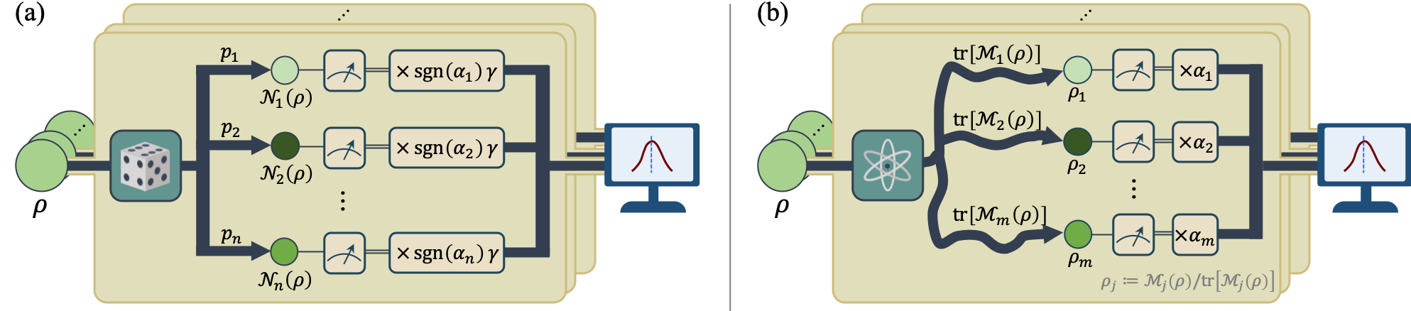
Figure 1: Difference between QPD and measurement-controlled post-processing. The task is to estimate the expectation value of an observable with respect to a state transformed by a Hermitian-preserving map without knowing the observable nor the state. (a) Estimating the expectation value with QPD. The action on the input state in each round is determined by classical random sampling, which is independent of the input state. (b) Estimating the expectation value with measurement-controlled post-processing. The action on the input state in each round is determined by quantum measurement governed by the Born rule, which takes the input state into consideration.

Measurement-controlled post-processing.— A Hermitian-preserving map, which maps Hermitian operators to Hermitian operators, can be written as a linear combination of CPTN maps. QPD simulates a Hermitian-preserving map using such a decomposition. For example, consider a decomposition of a Hermitian-preserving map ${\cal E}=\sum_{j}\alpha_{j}{\cal N}_{j}$, where each $\alpha_{j}$ is a real number and ${\cal N}_{j}$ is a CPTN map. To begin with, QPD samples a CPTN map from $\left\{{\cal N}_{j}\right\}$ with a probability distribution $p_{j}\coloneqq p({\cal N}_{j})\coloneqq|\alpha_{j}|/\sum_{j}|\alpha_{j}|$. Then, the sampled operation is applied to the input state $\rho$  followed by a one-shot measurement with the given observable $O$. When the sampled operation is ${\cal N}_{j}$, a coefficient ${\rm sgn}(\alpha_{j})\gamma$ will be multiplied to the outcome from the observable measurement, where $\gamma\coloneqq\sum_{j}|\alpha_{j}|$ and ${\rm sgn}$ denotes the sign function. The post-processing coefficient ensures that the final output has an expected value $\sum_{j}p_{j}{\rm sgn}(\alpha_{j})\gamma\operatorname{tr}[{\cal N}_{j}(\rho)O]=\operatorname{tr}\left[{\cal E}(\rho)O\right]$. After repeating the sampling, measurement, and post-processing for multiple rounds, we can get a fairly accurate estimation of $\operatorname{tr}\left[{\cal E}(\rho)O\right]$ by taking the average of the outputs from all rounds. The whole process is shown in Fig. 1(a).

Compared with physical operations, unphysical maps could lead to a higher sampling overhead in terms of the number of one-shot measurements, or equivalently, the number of input state copies required to achieve the desired accuracy Jiang et al. (2021); Regula et al. (2021). By Hoeffding’s inequality Hoeffding (1994), the number of one-shot measurements $M$ satisfying

$$M\geq\frac{2\gamma^{2}\|O\|_{\infty}^{2}\log\frac{2}{\delta}}{\varepsilon^{2}}=\gamma^{2}K(\delta,\varepsilon,O)$$ (1)

are needed to ensure that the final estimation is within an error $\varepsilon$ with a probability no less than $1-\delta$, where $K(\delta,\varepsilon,O)\coloneqq 2\|O\|_{\infty}^{2}\log\frac{2}{\delta}/\varepsilon^{2}$ is independent of the post-processing. The factor $\gamma=\sum_{j}|\alpha_{j}|$, which is the magnitude of the multiplying coefficients used in the post-processing, characterizes the sampling overhead of simulating ${\cal E}$ with the decomposition ${\cal E}=\sum_{j}\alpha_{j}{\cal N}_{j}$.

Note that in the above model of QPD, the action on the input state is controlled by a classical system. Which physical operation will be enacted in each round is resolved by a pre-determined classical probability distribution. As we are dealing with quantum information, there is no sense to limit the control system to a classical one. What we need is an operation that takes in an input state and outputs a state for the succeeding observable measurement and a classical value controlling the post-processing. The most general form of such a physical operation is known as a quantum instrument. We also note that quantum instrument was used in Ref. Buscemi et al. (2013) for simulating ideal two-point correlators.

A quantum instrument is a quantum operation that gives both classical and quantum outputs. Mathematically, it is described by a collection $\left\{{\cal M}_{j}\right\}$, where each ${\cal M}_{j}$ is a CPTN map and $\sum_{j}{\cal M}_{j}$ is CPTP Khatri and Wilde (2020). Given an initial state $\rho$, the quantum instrument outputs a measurement outcome $j$ and a corresponding post-measurement state $\rho_{j}\coloneqq{\cal M}_{j}(\rho)/\operatorname{tr}\left[{\cal M}_{j}(\rho)\right]$ with a probability $\operatorname{tr}\left[{\cal M}_{j}(\rho)\right]$ dependent on the input state. When the measurement outcome from the quantum instrument is $j$, we multiply a coefficient $\alpha_{j}$ to the value obtained from the one-shot observable measurement on the state $\rho_{j}$. Then, the expected value of the output after classical post-processing is $\sum_{j}\operatorname{tr}\left[{\cal M}_{j}(\rho)\right]\alpha_{j}\operatorname{tr}\left[\rho_{j}O\right]=\operatorname{tr}\left[\sum_{j}\alpha_{j}{\cal M}_{j}(\rho)O\right]$. As in QPD, we repeat these steps for multiple rounds to obtain an estimation of $\operatorname{tr}\left[\sum_{j}\alpha_{j}{\cal M}_{j}(\rho)O\right]$. We call this whole process measurement-controlled post-processing, which is visualized in Fig. 1(b).

In the example presented above, the map $\sum_{j}\alpha_{j}{\cal M}_{j}$ is the effective operation performed on the input state. While this decomposition looks a lot like the decomposition in QPD, the sampling overhead associated with it is $\alpha_{\max}\coloneqq\max_{j}|\alpha_{j}|$ instead of $\sum_{j}|\alpha_{j}|$. This is because $\alpha_{\max}$ is the largest magnitude among all the post-processing coefficients. Specifically, it can be directly verified by Hoeffding’s inequality that

$$M\geq\alpha_{\max}^{2}K(\delta,\varepsilon,O)$$ (2)

one-shot measurements, or equivalently, copies of the input state, are required to make sure the prediction has an error smaller than $\varepsilon$ with a probability no less than $1-\delta$.

The major distinction between QPD and measurement-controlled post-processing that leads to the difference in the expressions for sampling overheads is that QPD encodes a fixed probability distribution in the decomposition coefficients, whereas the latter does not impose such an artificial probability distribution on the measurement outcomes. Instead, the probability distribution $\left\{\operatorname{tr}\left[{\cal M}_{j}(\rho)\right]\right\}$ arises naturally from the the Born rule for the quantum measurement embedded in the CPTN maps constituting the quantum instrument, and the distribution varies from state to state.

Twisted channel for mathematical characterization.— To assist the analysis of measurement-controlled post-processing, we introduce what we call a twisted channel as its mathematical characterization. The effective operation $\sum_{j}\alpha_{j}{\cal M}_{j}$ can be written as $\alpha_{\max}\sum_{j}\alpha^{\prime}_{j}{\cal M}_{j}$, where the normalized coefficient $\alpha^{\prime}_{j}\coloneqq\alpha_{j}/\alpha_{\max}$ satisfies $|\alpha^{\prime}_{j}|\leq 1$. Then, the combination $\sum_{j}\alpha^{\prime}_{j}{\cal M}_{j}$ has a unit sampling overhead and $\sum_{j}|\alpha^{\prime}_{j}|{\cal M}_{j}$ is a CPTN map. Without loss of generality, we can require $\sum_{j}|\alpha^{\prime}_{j}|{\cal M}_{j}$ to be CPTP. This is because there exists a map ${\cal M}^{\prime}$ such that $\sum_{j}|\alpha^{\prime}_{j}|{\cal M}_{j}+2{\cal M}^{\prime}$ is CPTP. Then, we can add two terms ${\cal M}^{\prime}$ and $-{\cal M}^{\prime}$ into the combination $\sum_{j}\alpha^{\prime}_{j}{\cal M}_{j}$ without changing the map this combination represents for nor its sampling overhead. Absorbing $|\alpha^{\prime}_{j}|$ into each ${\cal M}_{j}$, we arrive at the following definition of a twisted channel .

Definition 1 (Twisted channel)

A twisted channel ${\cal T}$ is a linear map that can be written as ${\cal T}=\sum_{j}s_{j}{\cal M}_{j}$, where $s_{j}\in\left\{+1,-1\right\}$ and $\left\{{\cal M}_{j}\right\}$ is a quantum instrument.

A twisted channel is a map that, though not necessarily physical, can be simulated with unit sampling overhead using measurement-controlled post-processing with a quantum instrument. It is clear that the effective operation of measurement-controlled post-processing is simply a single twisted channel scaled by a coefficient that coincides with the sampling overhead. As measurement-controlled post-processing is more general than the classically controlled one, one twisted channel with a suitable scalar is enough for simulating any Hermitian-preserving map, and we formally prove this statement in the Appendix. On the other hand, one may decompose a Hermitian-preserving map into a linear combination of multiple twisted channels as in QPD, which corresponds to sampling multiple quantum instruments. It turns out that involving more quantum instruments does not result in a lower overhead. In other words, a single quantum instrument is all it needs to simulate an arbitrary Hermitian-preserving map with an optimal sampling overhead.

Theorem 2 (One quantum instrument is all you need)

Under measurement-controlled post-processing, any protocol that involves the sampling of multiple quantum instruments is equivalent to a protocol using a single quantum instrument in terms of the simulated map and the sampling overhead.

The proof of Theorem 2 can be found in the Appendix, where we show that any linear combination of twisted channels can be reduced to a scaled twisted channel without changing the sampling overhead.

Diamond norm as the simulation cost.— We have shown that in both QPD and measurement-controlled post-processing, a sampling overhead characterizing the required number of one-shot measurement rounds is associated with a decomposition of a Hermitian-preserving map. Considering that a Hermitian-preserving map’s decomposition is not unique, we define a Hermitian-preserving map’s simulation cost as the lowest possible sampling overhead associated with any its valid decomposition. Within measurement-controlled post-processing, the simulation cost of a Hermitian-preserving map ${\cal E}$ is defined as

$$\gamma_{\rm TC}\left({\cal E}\right)\coloneqq\min\left\{\alpha~{}\middle|~{}{\cal E}=\alpha{\cal T},~{}\alpha\geq 0,~{}{\cal T}\in{\rm TC}\right\},$$ (3)

where ${\rm TC}$ denotes the set of twisted channels.

The diamond norm, also known as the completely bounded trace norm, is a fundamental quantity in quantum information and efficiently computable by a semi-definite program (SDP) Kitaev (1997); Watrous (2018). It serves as a measure of distance between quantum channels and finds natural operational meanings in channel discrimination tasks Rosgen and Watrous (2005); Gilchrist et al. (2005). Given a Hermitian-preserving map ${\cal E}_{A\to B}$, its diamond norm is defined as

$$\left\|{\cal E}\right\|_{\diamond}\coloneqq\max_{\rho_{A^{\prime}A}}\left\|{\operatorname{id}}_{A^{\prime}}\otimes{\cal E}_{A\to B}(\rho_{A^{\prime}A})\right\|_{1},$$ (4)

where the optimization is over all states $\rho_{A^{\prime}A}$ and the dimension of the system $A^{\prime}$ is equal to the dimension of system $A$. The map ${\operatorname{id}}_{A^{\prime}}$ denotes the identity channel on the system $A^{\prime}$, and $\left\|\cdot\right\|_{1}$ is the trace norm.

For any Hermitian-preserving map that is proportional to a trace-preserving map, it has been shown in Ref. Regula et al. (2021) that its simulation cost using QPD is equal to its diamond norm Kitaev (1997). However, for general Hermitian-preserving maps, this equality between the cost and the diamond norm does not hold. In an extreme case, the simulation cost can be twice as large as the map’s diamond norm.

In Theorem 3, we show that this unpleasant gap between the cost in QPD and the diamond norm can be remedied. In particular, we prove that the simulation cost induced by the measurement-controlled post-processing is equal to the map’s diamond norm for any Hermitian-preserving map.

Theorem 3 (Diamond norm is the cost)

Let ${\cal E}_{A\to B}$ be an arbitrary Hermitian-preserving map. Then, its simulation cost using a twisted channel can be obtained by the following SDP:

$$\gamma_{\rm TC}({\cal E})= \min\big{\{}\alpha~{}\big{|}~{}J^{{\cal E}}=M^{+}-M^{-},~{}M^{\pm}\geq 0,$$

$$\qquad\qquad\operatorname{tr}_{B}\left[M^{+}+M^{-}\right]=\alpha\mathbbm{1}\big{\}},$$ (5)

where $J^{{\cal E}}$ is the Choi operator of ${\cal E}$. Furthermore, this cost is equal to the map’s diamond norm, i.e.,

$$\gamma_{\rm TC}({\cal E})=\|{\cal E}\|_{\diamond}.$$ (6)

The SDP in Eq. (3) follows from the fact that any twisted channel can be written as a difference between two CPTN maps because CPTN maps following the same coefficient in the decomposition can be grouped into a single CPTN map. A formal proof of this theorem is given in the Appendix.

Theorem 3 not only implies that measurement-controlled post-processing can simulate a Hermitian-preserving map at a cost much lower than QPD, but also establishes diamond norm as a universal quantity measuring the simulability of a Hermitian-preserving map.

From another perspective, the cost of simulating an unphysical map characterizes the map’s non-physicality Regula et al. (2021); Jiang et al. (2021). All conventional physical operations, i.e., CPTN maps, have unit simulation costs. Within the framework where classical post-processing is allowed, physical operations are extended to twisted channels. Intuitively, the more unphysical a map is, the more expensive it is to simulate this map with physical operations. In this sense, we treat non-physicality as a resource and twisted channels as free operations. Then, a map’s non-physicality can be quantified by robustness measures, which are widely used in quantum resource theories Chitambar and Gour (2019); Vidal and Tarrach (1999); Harrow and Nielsen (2003); Steiner (2003); Brandão (2007); Almeida et al. (2007); Napoli et al. (2016); Skrzypczyk and Linden (2019).

Here, we consider the absolute robustness Vidal and Tarrach (1999) of a Hermitian-preserving map ${\cal E}$, which we define as

$$R({\cal E})\coloneqq\min\left\{\lambda~{}\middle|~{}\frac{{\cal E}+\lambda{\cal T}}{1+\lambda}\in{\rm TC},~{}{\cal T}\in{\rm TC}\right\}.$$ (7)

It turns out that this robustness measure is equivalent to the diamond norm in the way that

$$\|{\cal E}\|_{\diamond}=2R({\cal E})+1$$ (8)

holds for all Hermitian-preserving maps ${\cal E}$. A proof of this equality can be found in the Appendix.

Advantages of twisted channels in practice.— Here, we study information recovering and processing as two examples of the twisted channels’ applications to demonstrate the advantage of quantum measurement over classical sampling in practical tasks.

Information recovering refers to the task that predicts the expectation value of an observable $O$ with respect to a quantum state $\rho$ given its noisy copies ${\cal N}(\rho)$, where the channel ${\cal N}$ represents the noise. This problem was proposed in Ref. Zhao et al. (2023), where the authors addressed it within a framework of classically sampling CPTP maps. This is equivalent to optimizing a Hermitian-preserving and trace-scaling map ${\cal D}$ so that $\operatorname{tr}\left[{\cal D}\circ{\cal N}(\rho)O\right]=\operatorname{tr}\left[\rho O\right]$, where a map is said to be trace-scaling if it is proportional to some trace-preserving map.

Here, we extend this framework to include general Hermitian-preserving maps, which can be simulated either by classically sampling CPTN maps using QPD or by a twisted channel realized through measurement-controlled post-processing. We compare the lowest sampling overheads incurred by these two methods to recover the desired expectation value in an example, and the results are presented in Fig. 2. In this example, the given observable is the sum of the four Pauli operators $X+Y+Z+I$. We consider three different types of noise: the amplitude damping noise ${\cal N}_{\rm AD}^{\epsilon}(\cdot)$ with Kraus operators $|0\rangle\!\langle 0|+\sqrt{1-\epsilon}|1\rangle\!\langle 1|$ and $\sqrt{\epsilon}|0\rangle\!\langle 1|$, the dephasing noise ${\cal N}_{\rm deph}^{\epsilon}$ with Kraus operators $\sqrt{1-\epsilon/2}I$ and $\sqrt{\epsilon/2}Z$, and the depolarizing noise ${\cal N}_{\rm depo}^{\epsilon}(\cdot)=(1-\epsilon)(\cdot)+\epsilon\operatorname{tr}[\cdot]I/2$. The parameter $\epsilon\in[0,1]$ indicates the noise level for all the three channels. It is observed in Fig. 2 that for all these noises, the twisted channel method incurs overheads significantly lower than those of QPD, and the gaps between them steadily enlarge as the noise level goes up.

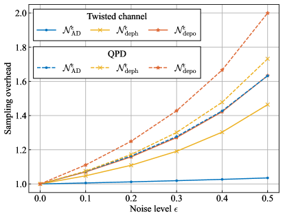
Figure 2: Comparison between sampling overheads of QPD and measurement-controlled post-processing for information recovering under common noises at different noise levels. The markers on the solid lines represent the overheads achieved by using twisted channels, i.e., measurement-controlled post-processing, and those on the dashed lines are the overheads achieved by QPD.

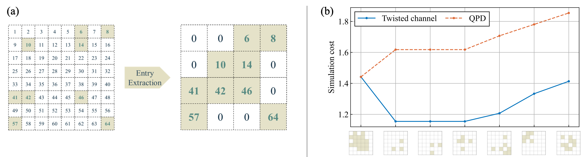
Figure 3: Illustration of entry extraction maps and a comparative evaluation of their implementation using QPD and the twisted channel method. (a) A typical instance of an entry extraction map, which converts an $8\times 8$ matrix into a $4\times 4$ matrix that comprises all the extracted entries while preserving their relative locations. (b) A plot comparing the costs of QPD and the twisted channel method across various entry extraction maps. All the maps share a common input dimension and are distinguished by the index sets they extract, as indicated on the horizontal axis.

The other application is the processing of quantum data, which involves a collection of tasks aimed at implementing extraction maps on input quantum states. Quantum algorithms have the potential to achieve quantum speedup owing to the vast information storage capabilities of quantum systems. However, this advantage also poses challenges in processing valuable information when quantum data contain a surplus of irrelevant details. To optimize the efficiency and accuracy of quantum algorithms, it is crucial to implement an extraction map that minimizes the spatial dimensions of quantum data while retaining as much useful information as possible. This is especially important for some quantum machine learning tasks. For example, in the quantum convolutional neural networks proposed in Ref. Cong et al. (2019), such operations are implemented by measurement-controlled unitaries, and hence are restricted to physical maps only.

Twisted channels can expand the range of applicable extraction to encompass unphyscial maps. We consider an elementary operation called the entry extraction map as an example. In particular, entry extraction maps extract entry-wise information of an input quantum state and blend these entries with zeros to form a new matrix while preserving the relative positions of the entries. Additionally, when an off-diagonal entry is extracted, its symmetrical counterpart must be extracted as well to maintain Hermiticity. The graphical illustration of an entry extraction map can be found in Fig. 3(a), and its mathematical definition is presented in the Appendix.

To showcase the efficiency of quantum measurement, we compare the simulation costs between QPD and the twisted channel method for several entry extraction maps. The input quantum data for these maps are fixed to $6\times 6$ matrices, while the output dimensions and indices sets extracted by these map are randomly selected. Fig. 3(b) illustrates that for all the selected extracting operations, measurement-controlled post-processing achieves the same or lower costs than QPD.

Quantum interference supplies the advantage.— The advantage of measurement-controlled post-processing over QPD is substantiated by the numerical results presented above. Consequently, it is pertinent to inquire about the underlying physical property that contributes to these enhancements. Here, we suggest that quantum interference is the key of such improvements.

Upon closer examination, the only difference between measurement-controlled post-processing and QPD lies in their respective methodologies of operation sampling. QPD first samples an operation according to a fixed priori probability distribution and then performs the sampled operation. On the other hand, measurement-controlled post-processing does not have such a priori probability distribution. As depicted in Fig. 1(b), it first applies an aggregate quantum operation to the input state, which creates interference between the paths leading to different measurement outcomes associated with different physical operations waiting to be sampled. The probability of getting each outcome is affected by the interference depending on the input state. Upon measurement, the quantum system collapses to an output state corresponding to one particular operation based on the adaptive probability distribution. Such dynamic assignment of probabilities makes interference the core ingredient for the enhancements brought by measurement-controlled post-processing.

Concluding remarks.— We demonstrate the power of quantum measurement in an important practical task by showing that quantum measurement results in a lower simulation cost of an unphysical operations compared with classical sampling. The simulation costs when quantum measurement is employed reduce to the well-known diamond norm for all Hermitian-preserving maps.

The measurement-controlled post-processing scheme can be extended to other scenarios in addition to simulating unphysical maps. More and more quantum algorithms and protocols consider classical randomness and post-processing as useful tools. Examples of use cases include circuit knitting Mitarai and Fujii (2021a); Piveteau and Sutter (2022), Hamiltonian simulation Campbell (2019); Faehrmann et al. (2022); Kiss et al. (2023), and quantum error correction Piveteau et al. (2021); Lostaglio and Ciani (2021); Suzuki et al. (2022). Whether quantum measurement can be used in place of classical sampling in these cases to further improve the performance is an interesting open problem for future work.

Acknowledgments.— The authors thank Mingrui Jing for fruitful discussions.

Appendix A Appendix A: One Quantum Instrument Is All You Need

Before we give a proof of Theorem 2, we first show that a single twisted channel scaled by a suitable coefficient is enough to simulate any Hermitian-preserving map.

Proposition 4

A linear map ${\cal E}$ can be written as $\alpha{\cal T}$ for a twisted channel ${\cal T}$ and a real number $\alpha$ if and only if it is Hermitian-preserving.

Proof.

For the “only if” part, we note that ${\cal T}$ is Hermitian-preserving as it is a linear combination of CPTN maps, which are Hermitian-preserving. Hence, $\alpha{\cal T}$ is a Hermitian-preserving map.

For the “if” part, we note that any Hermitian-preserving linear map ${\cal E}$ can be written as a linear combination of CPTN maps that constitute a quantum instrument, i.e., ${\cal E}=\sum_{j}\alpha_{j}{\cal N}_{j}$ for each ${\cal N}_{j}$ being CPTN and $\sum_{j}{\cal N}_{j}$ being CPTP (see Proposition 1 in Ref. Buscemi et al. (2013)). Denoting $\alpha_{\max}\coloneqq\max_{j}|\alpha_{j}|$ and $\alpha_{j}^{\prime}\coloneqq\alpha_{j}/\alpha_{\max}$, we have ${\cal E}=\alpha_{\max}\sum_{j}\alpha_{j}^{\prime}{\cal N}_{j}$. By definition, $|\alpha_{j}^{\prime}|\leq 1$ and thus each ${\cal M}_{j}\coloneqq|\alpha_{j}^{\prime}|{\cal N}_{j}$ is CPTN and so is $\sum_{j}{\cal M}_{j}$. Let ${\cal M}^{\prime}$ be a CPTN map such that $\sum_{j}{\cal M}_{j}+2{\cal M}^{\prime}$ is CPTP. Note that such a map always exists. Then, we can write the Hermitian-preserving map ${\cal E}$ as ${\cal E}=\alpha_{\max}\left(\sum_{j}s_{j}{\cal M}_{j}+{\cal M}^{\prime}-{\cal M}^{\prime}\right)$, where $s_{j}\coloneqq{\rm sgn}(\alpha_{j}^{\prime})$ denotes the sign of $\alpha_{j}^{\prime}$ and $\sum_{j}s_{j}{\cal M}_{j}+{\cal M}^{\prime}-{\cal M}^{\prime}$ is a twisted channel.     $\sqcap$$\sqcup$

Now we show that a single twisted channel is not only enough, but also optimal. That is, as stated in Theorem 2, allowing the sampling of multiple quantum instruments does not lower the sampling overhead of simulation.

Theorem 2

Under measurement-controlled post-processing, any protocol that involves the sampling of multiple quantum instruments is equivalent to a protocol using a single quantum instrument in terms of the simulated map and the sampling overhead.

A measurement-controlled post-processing protocol with multiple quantum instruments is described as a linear combination of twisted channels and its sampling overhead is the sum of the absolute values of the coefficients in the combination as in QPD. In the following lemma, we show that any linear combination of twisted channels can be rewritten as a single twisted channel scaled by the combination’s sampling overhead.

Lemma 5

For any linear combination of twisted channels $\sum_{j}\alpha_{j}{\cal T}_{j}$, there exists a single twisted channel ${\cal T}$ such that $\alpha{\cal T}=\sum_{j}\alpha_{j}{\cal T}_{j}$ for $\alpha=\sum_{j}|\alpha_{j}|$.

Proof.

Without loss of generality, we can assume that every $\alpha_{j}$ is positive because we can flip the sign of the corresponding twisted channel otherwise. Moreover, any twisted channel ${\cal T}=\sum_{j}s_{j}{\cal M}_{j}$ can be written as a difference between two CPTN maps that add up to a CPTP map, i.e., ${\cal T}={\cal T}^{+}-{\cal T}^{-}$, where ${\cal T}^{\pm}\coloneqq\sum_{s_{j}=\pm 1}{\cal M}_{j}$. Then, denoting $\sum_{j}\alpha_{j}$ by $\alpha$ and $\alpha_{j}/\alpha$ by $p_{j}$, the linear combination can be simplified as

$$\sum_{j}\alpha_{j}{\cal T}_{j}=\alpha\sum_{j}p_{j}({\cal T}_{j}^{+}-{\cal T}_{j}^{-})=\alpha\left({\cal W}^{+}-{\cal W}^{-}\right)$$ (9)

where ${\cal W}^{\pm}\coloneqq\sum_{j}p_{j}{\cal T}_{j}^{\pm}$. Note that $\sum_{j}p_{j}=1$, and ${\cal T}_{j}^{\pm}$ are CPTN, so ${\cal W}^{\pm}$ are also CPTN due to the convexity of the set of CPTN maps. Also, ${\cal W}^{+}+{\cal W}^{-}=\sum_{j}p_{j}({\cal T}_{j}^{+}+{\cal T}_{j}^{-})$ is CPTP because ${\cal T}_{j}^{+}+{\cal T}_{j}^{-}$ is CPTP for each $j$ and the set of CPTP maps is convex. That is, ${\cal W}^{+}-{\cal W}^{-}$ is a twisted channel.     $\sqcap$$\sqcup$

A scaled twisted channel $\alpha{\cal T}$ has a sampling overhead $|\alpha|$. On the other hand, a linear combination of twisted channels $\sum_{j}\alpha_{j}{\cal T}_{j}$ has a sampling overhead of $\sum_{j}|\alpha_{j}|$ as we need to classically sample the quantum instrument corresponding to each ${\cal T}_{j}$ as in QPD. Since Lemma 5 shows that for any such linear combination, there is always a scaled twisted channel $\alpha{\cal T}$ satisfying $\alpha{\cal T}=\sum_{j}\alpha_{j}{\cal T}_{j}$ and $\alpha=\sum_{j}|\alpha_{j}|$, we conclude that there exists a single quantum instrument (corresponds to ${\cal T}$) that simulates the same Hermitian-preserving map as sampling a set of quantum instruments (corresponds to $\left\{{\cal T}_{j}\right\}$) at the same overhead under measurement-controlled post-processing.

Appendix B Appendix B: Diamond Norm Is the Cost

The diamond norm of a Hermitian-preserving map ${\cal E}_{A\to B}$ is defined as

$$\left\|{\cal E}\right\|_{\diamond}\coloneqq\max_{\rho_{A^{\prime}A}}\left\|{\operatorname{id}}_{A^{\prime}}\otimes{\cal E}_{A\to B}(\rho_{A^{\prime}A})\right\|_{1},$$ (10)

where the optimization is over all states $\rho_{A^{\prime}A}$ and the dimension of the system $A^{\prime}$ is equal to the dimension of system $A$. The map ${\operatorname{id}}_{A^{\prime}}$ denotes the identity channel on the system $A^{\prime}$, and $\left\|\cdot\right\|_{1}$ is the trace norm. Here, we derive the SDP given in Theorem 3 for the cost of simulating any Hermitian-preserving map using a twisted channel, which happens to be an SDP for the map’s diamond norm as well.

Theorem 3

Let ${\cal E}_{A\to B}$ be an arbitrary Hermitian-preserving map. Then, its simulation cost using a twisted channel can be obtained by the following SDP:

$$\gamma_{\rm TC}({\cal E})=\min\big{\{}\alpha~{}\big{|}~{}J^{{\cal E}}=M^{+}-M^{-},~{}M^{\pm}\geq 0,~{}\operatorname{tr}_{B}\left[M^{+}+M^{-}\right]=\alpha\mathbbm{1}\big{\}},$$ (11)

where $J^{{\cal E}}$ is the Choi operator of ${\cal E}$. Furthermore, this cost is equal to the map’s diamond norm, i.e.,

$$\gamma_{\rm TC}({\cal E})=\|{\cal E}\|_{\diamond}.$$ (12)

Proof.

The simulation cost of a Hermitian-preserving map ${\cal E}$ with a twisted channel is the smallest possible $\alpha$ such that $\alpha{\cal T}={\cal E}$ for a twisted channel ${\cal T}$ and $\alpha\geq 0$. In the proof of Lemma 5, we showed that any twisted channel can be represented as a difference between two CPTN maps, which leads to the following formulation of the simulation cost:

$$\gamma_{\rm TC}\left({\cal E}\right)=\min\left\{\alpha~{}\middle|~{}{\cal E}=\alpha({\cal M}^{+}-{\cal M}^{-}),~{}\alpha\geq 0,~{}{\cal M}^{\pm}~{}\text{are CPTN},~{}{\cal M}^{+}+{\cal M}^{-}~{}\text{is CPTP}\right\}.$$ (13)

By the Choi-Jamiołkowski isomorphism Jamiołkowski (1972); Choi (1975), we can write the minimization above using the Choi operators of ${\cal E}$ and ${\cal M}^{\pm}$. A linear map ${\cal N}_{A\to B}$’s Choi operator is defined as

$$J^{\cal N}_{AB}\coloneqq{\operatorname{id}}_{A}\otimes{\cal N}_{A^{\prime}\to B}(|\Gamma\rangle\!\langle\Gamma|_{AA^{\prime}}),$$ (14)

where $|\Gamma\rangle_{AA^{\prime}}\coloneqq\sum_{j=0}^{d_{A}}|j\rangle_{A}|j\rangle_{A^{\prime}}$ is the unnormalized maximally entangled state, $d_{A}$ is the dimension of the Hilbert space ${\cal H}_{A}$ associated to system $A$, and ${\cal H}_{A^{\prime}}$ is isomorphic to ${\cal H}_{A}$. The linear map ${\cal N}_{A\to B}$ is completely positive if and only if its Choi operator is positive. It is trace-presrving if and only if $\operatorname{tr}_{B}\left[J^{\cal N}_{AB}\right]=\mathbbm{1}_{A}$, and it is trace-non-increasing if and only if $\operatorname{tr}_{B}\left[J^{\cal N}_{AB}\right]\leq\mathbbm{1}_{A}$. Then, Eq. (13) can be rewritten as

$$\gamma_{\rm TC}\left({\cal E}\right)=\min\left\{\alpha~{}\middle|~{}J^{{\cal E}}=\alpha\left(J^{{\cal M}^{+}}-J^{{\cal M}^{-}}\right),~{}\alpha\geq 0,~{}J^{{\cal M}^{\pm}}\geq 0,~{}\operatorname{tr}_{B}\left[J^{{\cal M}^{\pm}}\right]\leq\mathbbm{1}_{A},~{}\operatorname{tr}_{B}\left[J^{{\cal M}^{+}}+J^{{\cal M}^{-}}\right]=\mathbbm{1}_{A}\right\}.$$ (15)

Denoting $M^{\pm}\coloneqq\alpha J^{{\cal M}^{\pm}}$ and take them into the equation above, we obtain the following SDP:

$$\gamma_{\rm TC}\left({\cal E}\right)=\min\left\{\alpha~{}\middle|~{}J^{{\cal E}}=M^{+}-M^{-},~{}\alpha\geq 0,~{}M^{\pm}\geq 0,~{}\operatorname{tr}_{B}\left[M^{\pm}\right]\leq\alpha\mathbbm{1}_{A},~{}\operatorname{tr}_{B}\left[M^{+}+M^{-}\right]=\alpha\mathbbm{1}_{A}\right\}.$$ (16)

Note that both $\alpha\geq 0$ and $\operatorname{tr}_{B}\left[M^{\pm}\right]\leq\alpha\mathbbm{1}_{A}$ are already implied by $M^{\pm}\geq 0$ and $\operatorname{tr}_{B}\left[M^{+}+M^{-}\right]=\alpha\mathbbm{1}_{A}$. Thus, we can trim this SDP to arrive at the one stated in Theorem 3:

$$\gamma_{\rm TC}\left({\cal E}\right)=\min\left\{\alpha~{}\middle|~{}J^{{\cal E}}=M^{+}-M^{-},~{}M^{\pm}\geq 0,~{}\operatorname{tr}_{B}\left[M^{+}+M^{-}\right]=\alpha\mathbbm{1}_{A}\right\}.$$ (17)

For the equivalence between $\gamma_{\rm TC}$ and the diamond norm, we refer to Ref. Regula et al. (2021), where the authors show that the SDP in Eq. (17) is an SDP for the diamond norm. This completes the proof of Theorem 3.     $\sqcap$$\sqcup$

In the main text, we also define a related quantity, that is, the absolute robustness $R({\cal E})$ of a Hermitian-preserving map ${\cal E}$:

$$R({\cal E})\coloneqq\min\left\{\lambda~{}\middle|~{}\frac{{\cal E}+\lambda{\cal T}}{1+\lambda}\in{\rm TC},~{}{\cal T}\in{\rm TC}\right\}.$$ (18)

Below, we show that there is a constant relation between the diamond norm and the absolute robustness. This establishes the equivalence between these two quantities over all Hermitian-preserving maps.

Proposition 6

For any Hermitian-preserving map ${\cal E}$, it holds that

$$R({\cal E})=\frac{\left\|{\cal E}\right\|_{\diamond}-1}{2}.$$ (19)

Proof.

Let $\Phi$ be a twisted channel such that $\Psi\coloneqq({\cal E}+R({\cal E})\Phi)/(1+R({\cal E}))\in{\rm TC}$. Then we can write ${\cal E}$ as ${\cal E}=(1+R({\cal E}))\Psi-R({\cal E})\Phi$, which is a valid decomposition of ${\cal E}$ into twisted channels. The sampling overhead associated with this decomposition is $1+2R({\cal E})$. Since $\left\|{\cal E}\right\|_{\diamond}=\gamma_{\rm TC}({\cal E})$ is the minimized sampling overhead over all possible decompositions, we arrive at $\left\|{\cal E}\right\|_{\diamond}\leq 1+2R({\cal E})$, or, equivalently, $R({\cal E})\geq(\left\|{\cal E}\right\|_{\diamond}-1)/2$.

On the other hand, suppose ${\cal T}$ is a twisted channel that simulates ${\cal E}$ with the optimal sampling overhead $\left\|{\cal E}\right\|_{\diamond}$, i.e., ${\cal E}=\left\|{\cal E}\right\|_{\diamond}{\cal T}$. Then, we can write ${\cal T}$ as

$${\cal T}=\frac{{\cal E}+s(-{\cal T})}{1+s},$$ (20)

where $s\coloneqq\left(\left\|{\cal E}\right\|_{\diamond}-1\right)/2$. As both ${\cal T}$ and $-{\cal T}$ are twisted channels, Eq. (20) is a feasible solution to the minimization problem that defines the robustness in Eq. (18). Thus, we have $R({\cal E})\leq s=(\left\|{\cal E}\right\|_{\diamond}-1)/2$.

Now we have established that $\left(\left\|{\cal E}\right\|_{\diamond}-1\right)/2\leq R({\cal E})\leq\left(\left\|{\cal E}\right\|_{\diamond}-1\right)/2$. Therefore, we conclude that $R({\cal E})=(\left\|{\cal E}\right\|_{\diamond}-1)/2$ for any Hermitian-preserving map ${\cal E}$.     $\sqcap$$\sqcup$

Appendix C Appendix C: Entry Extraction

Entry extraction maps extract entry-wise information of an input quantum state and mix these entries with zeros to form an output matrix for further processing. Below is the mathematical definition of an entry extraction map.

Definition 7

Suppose ${\cal I}=\{i_{k}\}_{k=0}^{d^{\prime}-1}\subseteq[d]$ is an indexed set with increasing order. For a set of indexed pairs $A\subseteq\{(j,k)\mid j\leq k,~{}i_{j},i_{k}\in{\cal I}\}$, the corresponding entry extraction map ${\cal E}$ is defined as

$${\cal E}\mathrel{\mathop{\mathchar 58\relax}}{{\mathbb{C}}}^{d\times d}\to{{\mathbb{C}}}^{d^{\prime}\times d^{\prime}}\mathrel{\mathop{\mathchar 58\relax}}H=\sum_{j,k=0}^{d-1}H_{jk}|j\rangle\!\langle k|_{d}\mapsto\sum_{(j,k)\in A\cup A^{*}}H_{i_{j}i_{k}}|j\rangle\!\langle k|_{d^{\prime}},$$ (21)

where $A^{*}=\{(k,j)~{}|~{}(j,k)\in A\}$, $|j\rangle\!\langle k|_{d}\in{{\mathbb{C}}}^{d\times d}$ and $|j\rangle\!\langle k|_{d^{\prime}}\in{{\mathbb{C}}}^{d^{\prime}\times d^{\prime}}$.

Note that the Choi representation of ${\cal E}$ is

$$J^{\cal E}=\sum_{j,k=0}^{d-1}|j\rangle\!\langle k|_{d}\otimes{\cal E}(|j\rangle\!\langle k|_{d})=\sum_{(j,k)\in A\cup A^{*}}|i_{j}\rangle\!\langle i_{k}|_{d}\otimes|j\rangle\!\langle k|_{d^{\prime}}.$$ (22)

Then $J^{\cal E}=\left(J^{\cal E}\right)^{\dagger}$ by the symmetry of $A\cup A^{*}$, implying that ${\cal E}$ is Hermitian-preserving.

References

- Lund et al. (2017) A. P. Lund, M. J. Bremner, and T. C. Ralph, npj Quantum Information 3, 15 (2017).
- Hangleiter and Eisert (2023) D. Hangleiter and J. Eisert, Reviews of Modern Physics 95, 035001 (2023).
- Terhal and DiVincenzo (2004) B. M. Terhal and D. P. DiVincenzo, Quantum Information & Computation 4, 134–145 (2004).
- Arute et al. (2019) F. Arute, K. Arya, R. Babbush, D. Bacon, J. C. Bardin, R. Barends, R. Biswas, S. Boixo, F. G. Brandao, D. A. Buell, et al., Nature 574, 505 (2019).
- Zhong et al. (2020) H.-S. Zhong, H. Wang, Y.-H. Deng, M.-C. Chen, L.-C. Peng, Y.-H. Luo, J. Qin, D. Wu, X. Ding, Y. Hu, et al., Science 370, 1460 (2020).
- Wu et al. (2021) Y. Wu, W.-S. Bao, S. Cao, F. Chen, M.-C. Chen, X. Chen, T.-H. Chung, H. Deng, Y. Du, D. Fan, et al., Physical Review Letters 127, 180501 (2021).
- Madsen et al. (2022) L. S. Madsen, F. Laudenbach, M. F. Askarani, F. Rortais, T. Vincent, J. F. Bulmer, F. M. Miatto, L. Neuhaus, L. G. Helt, M. J. Collins, et al., Nature 606, 75 (2022).
- Peres (1996) A. Peres, Physical Review Letters 77, 1413 (1996).
- Horodecki et al. (1996) M. Horodecki, P. Horodecki, and R. Horodecki, Physics Letters A 223, 1 (1996).
- Gühne and Tóth (2009) O. Gühne and G. Tóth, Physics Reports 474, 1 (2009).
- Temme et al. (2017) K. Temme, S. Bravyi, and J. M. Gambetta, Physical Review Letters 119, 180509 (2017).
- Jiang et al. (2021) J. Jiang, K. Wang, and X. Wang, Quantum 5, 600 (2021).
- Horodecki and Ekert (2002) P. Horodecki and A. Ekert, Physical Review Letters 89, 127902 (2002).
- Regula et al. (2021) B. Regula, R. Takagi, and M. Gu, Quantum 5, 522 (2021).
- Wei et al. (2023) F. Wei, Z. Liu, G. Liu, Z. Han, X. Ma, D.-L. Deng, and Z. Liu, arXiv:2308.07956 (2023).
- Endo et al. (2018) S. Endo, S. C. Benjamin, and Y. Li, Physical Review X 8, 031027 (2018).
- Takagi (2021) R. Takagi, Physical Review Research 3, 033178 (2021).
- Piveteau et al. (2022) C. Piveteau, D. Sutter, and S. Woerner, npj Quantum Information 8, 12 (2022).
- Van Den Berg et al. (2023) E. Van Den Berg, Z. K. Minev, A. Kandala, and K. Temme, Nature Physics 19, 1116 (2023).
- Wang et al. (2022) K. Wang, Z. Song, X. Zhao, Z. Wang, and X. Wang, npj Quantum Information 8, 52 (2022).
- Yuan et al. (2023) X. Yuan, B. Regula, R. Takagi, and M. Gu, arXiv:2303.00955 (2023).
- Buscemi et al. (2013) F. Buscemi, M. Dall’Arno, M. Ozawa, and V. Vedral, arXiv:1312.4240 (2013).
- Note (1) As a sampled operation could be a CPTN map, it acting on the input state should give out a normalized state . However, a CPTN map is implemented by measurement and post-selection, and is exactly the success probability of implementing . This probability cancels out the normalization factor in the output state. For this reason, when analyzing QPD, we can ignore the normalization factor as in Fig. 1(a).
- Hoeffding (1994) W. Hoeffding, in The Collected Works of Wassily Hoeffding (Springer, 1994) pp. 409–426.
- Khatri and Wilde (2020) S. Khatri and M. M. Wilde, arXiv:2011.04672 (2020).
- Note (2) A set of operations similar to twisted channels has been noted in Ref. Piveteau and Sutter (2022) inspired by Ref. Mitarai and Fujii (2021b, a) for the task of circuit knitting. This set is introduced as a generalization of the set of CPTN maps to be used for classical sampling under the conventional QPD framework. In this work, we are taking an inherently different approach by replacing the classical sampling with quantum measurement, from which a twisted channel naturally arises.
- Kitaev (1997) A. Y. Kitaev, Russian Mathematical Surveys 52, 1191 (1997).
- Watrous (2018) J. Watrous, The Theory of Quantum Information (Cambridge University Press, 2018).
- Rosgen and Watrous (2005) B. Rosgen and J. Watrous, in 20th Annual IEEE Conference on Computational Complexity (CCC’05) (2005) pp. 344–354.
- Gilchrist et al. (2005) A. Gilchrist, N. K. Langford, and M. A. Nielsen, Physical Review A 71, 062310 (2005).
- Chitambar and Gour (2019) E. Chitambar and G. Gour, Reviews of Modern Physics 91, 025001 (2019).
- Vidal and Tarrach (1999) G. Vidal and R. Tarrach, Physical Review A 59, 141 (1999).
- Harrow and Nielsen (2003) A. W. Harrow and M. A. Nielsen, Physical Review A 68, 012308 (2003).
- Steiner (2003) M. Steiner, Physical Review A 67, 054305 (2003).
- Brandão (2007) F. G. S. L. Brandão, Physical Review A 76, 030301 (2007).
- Almeida et al. (2007) M. L. Almeida, S. Pironio, J. Barrett, G. Tóth, and A. Ac\́mathbf{i}n, Physical Review Letters 99, 040403 (2007).
- Napoli et al. (2016) C. Napoli, T. R. Bromley, M. Cianciaruso, M. Piani, N. Johnston, and G. Adesso, Physical Review Letters 116, 150502 (2016).
- Skrzypczyk and Linden (2019) P. Skrzypczyk and N. Linden, Physical Review Letters 122, 140403 (2019).
- Zhao et al. (2023) X. Zhao, B. Zhao, Z. Xia, and X. Wang, Quantum 7, 978 (2023).
- Cong et al. (2019) I. Cong, S. Choi, and M. D. Lukin, Nature Physics 15, 1273 (2019).
- Mitarai and Fujii (2021a) K. Mitarai and K. Fujii, Quantum 5, 388 (2021a).
- Piveteau and Sutter (2022) C. Piveteau and D. Sutter, arXiv:2205.00016 (2022).
- Campbell (2019) E. Campbell, Physical Review Letters 123, 070503 (2019).
- Faehrmann et al. (2022) P. K. Faehrmann, M. Steudtner, R. Kueng, M. Kieferova, and J. Eisert, Quantum 6, 806 (2022).
- Kiss et al. (2023) O. Kiss, M. Grossi, and A. Roggero, Quantum 7, 977 (2023).
- Piveteau et al. (2021) C. Piveteau, D. Sutter, S. Bravyi, J. M. Gambetta, and K. Temme, Physical Review Letters 127, 200505 (2021).
- Lostaglio and Ciani (2021) M. Lostaglio and A. Ciani, Physical Review Letters 127, 200506 (2021).
- Suzuki et al. (2022) Y. Suzuki, S. Endo, K. Fujii, and Y. Tokunaga, PRX Quantum 3, 010345 (2022).
- Mitarai and Fujii (2021b) K. Mitarai and K. Fujii, New Journal of Physics 23, 023021 (2021b).
- Jamiołkowski (1972) A. Jamiołkowski, Reports on Mathematical Physics 3, 275 (1972).
- Choi (1975) M.-D. Choi, Linear Algebra and Its Applications 10, 285 (1975).