Asymptotic symmetries of projectively compact order one Einstein manifolds

Abstract

We show that the boundary of a projectively compact Einstein manifold of dimension $n$ can be extended by a line bundle naturally constructed from the projective compactification. This extended boundary is such that its automorphisms can be identified with asymptotic symmetries of the compactification. The construction is motivated by the investigation of a new curved orbit decomposition for a $n+1$ dimensional manifold which we prove results in a line bundle over a projectively compact order one Einstein manifolds.

1 Introduction

In the study of objects living on non-compact manifolds it is often enlightening to try to make sense of their asymptotics. Curved orbit decompositions arising from holonomy reductions of (normal) Cartan geometries, as first studied in full generality in [ČGH14], provide a fascinating framework in which one can seemingly make sense of the asymptotics of geometric structures themselves. In many interesting cases, the orbit decomposition has a large open orbit $\mathcal{O}$ equipped with a certain geometric structure, e.g. an Einstein metric. Its complement can then be viewed as a boundary “at infinity” and splits into pieces endowed with other geometries that one may interpret as “limits” of the structure of $\mathcal{O}$.

Defining and studying the asymptotics of pseudo-Riemannian manifolds $(M,g)$ is of particular interest due to their importance in physics. For instance, conformal compactification is key for the formulation of a notion of isolated system in General Relativity [Ger77, PR84, Fra04, Val16]. It is also a way to approach the study of the asymptotic behaviour to partial differential equations on non-compact pseudo-Riemannian manifolds, see for instance [GLW15, CG18, MN04, Nic16, BGN23, MN09] in the conformal case or [Bor21] in the projective case, for examples of ideas and work in this direction.

In [ČGH12, ČGH14, ČGM14, ČG14, ČG16, FG18], a specific type of holonomy reduction of projective geometries is studied that gives rise to an Einstein metric on the open orbit, suggesting that projective geometry could play an important role in understanding their asymptotics. This is intimately related to the notion of projectively compact metric of order $\alpha$ introduced by Čap–Gover in [ČG14]. The order of a projectively compact metric is related to its volume asymptotics, and can a priori take any positive real value. For Einstein metrics, the cases $\alpha=1$ (vanishing scalar curvature) and $\alpha=2$ (non-vanishing scalar curvature) are the most relevant. Both cases were thoroughly investigated by Čap–Gover in [ČG14]. In particular, it is shown in this reference that, for projectively compact Einstein metrics of order $1$, this notion coincides with asymptotic flatness at spatial infinity as introduced by Ashtekar and Romano in [AR92], however with the restriction that only spacetime with vanishing mass aspect can be obtained in this way.

Asymptotic flatness at spatial infinity is by now a classical subject in general relativity, see e.g. [BS82, CD11, MK21, CGW23]. A physically important feature of these spacetimes is their asymptotic symmetry group: the – infinite dimensional – Spi group of [AR92]. The identification of spatial infinity with projective compactifications of order 1 however presents us with a conundrum: at null infinity, the group of asymptotic symmetry (the BMS group of [BVM62, Sac62]) can be identified with the automorphisms of the boundary geometry [Ger77, Ash15, DGH14] and act on the induced Cartan geometry [Her20, Her22a, Her22] encoding the radiative data. On the other hand the boundary geometry of projective compactification of order 1 of an Einstein metric is again a normal projective geometry with a holonomy reduction corresponding to projective compactification of order $2$ of an Einstein metric [ČG14] and thus necessarily has a finite dimensional group of automorphisms. So how exactly does the Spi group of Ashtekar–Romano plays a role in the projective compactification picture?

In this work we wish to resolve this tension by introducing an extended boundary at spatial infinity. In doing so, we follow the footsteps of Ashtekar–Hansen [AH78]. We will show that this idea fits perfectly with, and extends, the notion of projective compactification. The properties of this boundary parallel exactly that of null infinity: its geometry is not rigid and the corresponding group of automorphisms 1) coincides with the Spi group, 2) acts on a space of induced Cartan geometry encoding some asymptotic gravitational data. We also obtain a similar structure at time like infinity. In order to introduce and motivate this step, we will study a closely related curved orbit decomposition of Cartan geometries [ČGH14] generalising the work of Cap–Gover [ČG14]. The majority of this article will in fact be dedicated to the discussion of the curved version of a flat model discussed in great detail by Figueroa-O’Farrill and collaborators in [FHPS22]. This homogeneous model generalises the projectively compactified 4D model $\mathbb{R}\text{P}^{4}$ to a 5D model $\mathbb{R}\text{P}^{5}\setminus\{pt\}\simeq\mathbb{R}\times\mathbb{R}\text{P}^{4}$ fibering over the usual projective compactification.

$$\begin{array}[]{cccccc}\mathbb{R}\text{P}^{5}\setminus\{pt\}&\simeq&\left(\mathbb{R}\times M^{4}\right)&\sqcup&\left(\textrm{Ti}^{4}\sqcup\mathscr{I}^{3}\sqcup\textrm{Spi}^{4}\right)\\[10.00002pt] \downarrow&&\downarrow&&\downarrow\\[10.00002pt] \mathbb{R}\text{P}^{4}&\simeq&M^{4}&\sqcup&\left(H^{3}\sqcup S^{2}\sqcup dS^{3}\right).\end{array}$$ (1.1)

This orbit decomposition will be discussed in more detail (and generic dimension) in the core of this article, however we summarise here its essential features: while the action of the Poincaré group has a trivial action along the fibres $\mathbb{R}\times M^{4}\to M^{4}$ over Minkowski space, it has a non-trivial action over the extended boundary $\textrm{Ti}^{4}\sqcup\mathscr{I}^{3}\sqcup\textrm{Spi}^{4}$:

$$\begin{array}[]{ccccccc}\textrm{Ti}^{4}&\simeq&\frac{\text{ISO}(1,3)}{\mathbb{R}^{3}\rtimes\text{SO}(3)}&\to&H^{3}&\simeq&\frac{\text{SO}(1,3)}{\text{SO}(3)}\\[10.00002pt] \mathscr{I}^{3}&\simeq&\frac{\text{ISO}(1,3)}{\mathbb{R}^{3}\rtimes(\mathbb{R}^{*}\times\text{ISO}(2))}&\to&S^{2}&\simeq&\frac{\text{SO}(1,3)}{\mathbb{R}^{2}\rtimes(\mathbb{R}^{*}\times\text{SO}(2))}\\[10.00002pt] \textrm{Spi}^{4}&\simeq&\frac{\text{ISO}(1,3)}{\mathbb{R}^{3}\rtimes\text{SO}(1,2)}&\to&dS^{3}&\simeq&\frac{\text{SO}(1,3)}{\text{SO}(1,2)}.\par\end{array}$$ (1.2)

This points to the possibility of a non trivial geometrical extension of the boundary geometry of projectively compactified order 1 Einstein metrics. We shall prove in this article that this intuition is correct.

The article is organised as follows. In Section 2 we recall the elements of projective tractor calculus that we will need and discuss in more details the homogeneous model (1.1). In Section 3 we detail the different curved orbits of the corresponding holonomy reduction, under suitable assumptions this results in a line bundle $M\to\mathcal{Q}$. In Section 4 we prove that the open curved orbit $\mathcal{O}$ is of the form $\mathbb{R}\times\mathcal{Q}_{\mathcal{O}}$ where $\mathcal{Q}_{\mathcal{O}}$ is canonically endowed with an Einstein metric. We then prove, in Section 5, that as a submanifold of $\mathcal{Q}$, this is projectively compact of order $1$ with boundary $\mathcal{H}$. In Section 6 we investigate the induced geometry of the extended boundary $\Sigma\to\mathcal{H}$, first as a submanifold of $M\to\mathcal{Q}$ and then a natural extension of $\mathcal{H}\subset\mathcal{Q}$. Finally, in Section 7, we discuss asymptotic symmetries and their action on the extended boundary.

2 Projective tractors and the homogeneous model

It should be understood that all affine connections on the tangent bundle are torsion-free.

We make extensive use of the Penrose abstract index notation [PR84]. In index notation, tractor indices (see below) will be denoted by capital Latin letters, $A,B,C\dots,$.

The signature of a bilinear form will be written $(q,p)$: “$q$ ‘$-$’s and $p$ ‘$+$’s”.

2.1 Projective tractor calculus

We here review the elements of projective tractor calculus that we will need in the rest of the article.

Let $M$ be a manifold of dimension $n+1$ endowed with an equivalence class of projectively equivalent torsion-free connections $[\nabla]$. It is a standard result that two torsion-free affine connections $\hat{\nabla}$ and $\nabla$ are projectively equivalent if and only if there is a 1-form $\Upsilon_{a}$ such that for any vector field $\xi^{b}$:

$$\hat{\nabla}_{a}\xi^{b}=\nabla_{a}\xi^{b}+\Upsilon_{a}\xi^{b}+\Upsilon_{c}\xi^{c}\delta_{a}^{b}.$$

We will use $\hat{\nabla}=\nabla+\Upsilon$ as shorthand for this condition.

We denote by $\mathcal{E}(w)$ the associated vector bundle to the frame bundle $P^{1}(M)$ determined by the $1$-dimensional representation of $GL_{n+1}(\mathbb{R})$:

$$A\mapsto\lvert\det{A}\rvert^{\frac{w}{n+2}}.$$

Sections of this bundle will be called projective densities of weight $w$. Their definition is so that for any $\sigma\in\Gamma(\mathcal{E}(w))$ under the projective change of connection $\hat{\nabla}=\nabla+\Upsilon$,

$$\hat{\nabla}\sigma=\nabla\sigma+w\Upsilon\sigma.$$

For any vector bundle $\mathcal{B}$ with base $M$, we will write: $\mathcal{B}(w)=\mathcal{B}\otimes\mathcal{E}(w)$ and we will say that sections of $\mathcal{B}(w)$ are of weight $w$.

Let $G=\textnormal{PGL}(n+2,\mathbb{R})$ and $H=(\mathbb{R}^{n+1})^{*}\rtimes GL(n+1,\mathbb{R})$ the isotropy subgroup of a given line. The class $[\nabla]$ determines a reduction of the second-order frame bundle $P^{2}(M)$ to a $H$-principle bundle $P$, on which there is a unique normal Cartan connection $\omega$ [Car24, Kob95]; this is a normal projective geometry modeled on projective geometry as described in [Sha97].

The standard (projective) tractor bundle, $\mathcal{T}$ can be defined as the associated vector bundle to $P$ determined by the restriction to $H$ of the $(n+2)$-dimensional representation of $G$ given by: $A\mapsto\lvert\det A\rvert^{-\frac{1}{n+2}}A$. The Cartan connection $\omega$ induces a linear connection $\nabla^{\mathcal{T}}$ on $\mathcal{T}$.

The bundle $\mathcal{T}$ fits into a canonical short exact sequence of vector bundles:

A choice of connection in the projective class $[\nabla]$ provides a non-canonical isomorphism $\mathcal{T}\simeq\mathcal{E}(-1)\oplus TM(-1)$, described above by the non-canonical maps $Y$ and $W$. When thinking of these maps as sections of $\mathcal{T}^{*}\otimes\mathcal{E}(-1)$ and $T^{*}M(1)\otimes\mathcal{T}$ respectively, they transform under change of connection $\hat{\nabla}=\nabla+\Upsilon$ according to:

$$\hat{Y}_{A}=Y_{A}-\Upsilon_{a}Z^{a}_{A},\quad\widehat{W}^{A}_{a}=W^{A}_{a}+\Upsilon_{a}X^{A}.$$ (2.1)

Fixing a choice of connection $\nabla$ in the projective class, sections of the standard tractor bundle will be written:

$$T^{A}=\xi^{a}W_{a}^{A}+\rho X^{A},$$

similar expressions will be used with sections of tensor powers of the tractor bundle.

The dual tractor bundle $\mathcal{T}^{*}$ is usually identified with the first jet prolongation $J^{1}\mathcal{E}(1)$ of the weight $1$ projective density bundle [BEG94]. This description has the advantage of being more direct than the principal bundle approach outlined above, and is independent of the projective structure. In addition, it allows for straightforward comparisons of tractors on different manifolds; in particular, tractors in the “bulk” and on distinguished hypersurfaces.

We also recall from [BEG94] the standard decomposition of the curvature tensor $R_{ab\phantom{c}d}^{\phantom{ab}c}$:

$$R_{ab\phantom{c}d}^{\phantom{ab}c}=W_{ab\phantom{c}d}^{\phantom{ab}c}+2\delta^{c}_{[a}P_{b]d}+\beta_{ab}\delta^{c}_{d},$$

where the Weyl tensor $W$ is trace-free and $P_{ab}$ is the projective Schouten tensor. It is easily verified that:

$$nP_{ab}= R_{ab}+\beta_{ab},\quad\beta_{ab}=-\frac{2}{n+2}R_{[ab]}=-P_{[ab]},$$

where $R_{ab}=R_{da\phantom{d}b}^{\phantom{da}d}$ is the Ricci tensor. The tensor $\beta_{ab}$ can be thought of as the curvature tensor of the density bundle $\mathcal{E}(1)$.

A connection $\nabla$ is said to be special if it preserves a nowhere vanishing density $\sigma$. In this case $\beta_{ab}=0$ (in particular all density bundles are flat) and we say that $\nabla$ is the scale determined by $\sigma$. Even when it does not preserve a nowhere vanishing density, we will refer to a choice of connection in the class as a choice of scale.

Having fixed a projective connection $\nabla$ in the class, and split the short-exact sequence, the action of the normal Cartan connection can be summarised conveniently by the relations:

$$\nabla_{a}X^{A}=W^{A}_{a},\quad\nabla_{a}W^{B}_{b}=-P_{ab}X^{B},\quad\nabla_{a}Y_{A}=P_{ab}Z^{b}_{A},\quad\nabla_{a}Z^{b}_{B}=-\delta_{a}^{b}Y_{B}.$$ (2.2)

The tractor curvature, defined by, the identity $\Omega_{ab\phantom{C}D}^{\phantom{ab}C}T^{D}=2\nabla_{[a}\nabla_{b]}T^{C}$, is known to be given in an arbitrary scale by:

$$\Omega_{ab\phantom{C}D}^{\phantom{ab}C}=W_{ab\phantom{c}d}^{\phantom{ab}c}W^{C}_{c}Z^{d}_{D}-Y_{abd}X_{C}Z^{d}_{D}$$ (2.3)

Where: $Y_{abd}=2\nabla_{[a}P_{b]d}$ is the projective Cotton tensor.

A projective class $[\nabla]$ is said to be metric, if it admits a solution $\zeta^{ab}\in\Gamma(S^{2}(T^{*}M)(-2))$ to the Mikeš-Sinjukov metrisability equation [Mik96, Sin79]:

$$\textnormal{trace-free}\left(\nabla_{c}\zeta^{ab}\right)=0,$$

or equivalently $\nabla_{c}\zeta^{ab}=2\delta^{(a}_{c}\lambda^{b)}$ for some $\lambda^{a}$. Solutions of this equation have been shown [EM08, FG18] to be in one-to-one correspondence with tractors $H^{AB}$ that satisfy:

$$\nabla_{c}H^{AB}+\frac{2}{n+1}X^{(A}W_{cE\phantom{B}F}^{\phantom{cE}B)}H^{EF}=0,$$ (2.4)

where $W_{cE\phantom{B}F}^{\phantom{cE}B}=Z^{c}_{C}\Omega_{ce\phantom{B}F}^{\phantom{ce}B}$ and $\Omega_{ce\phantom{B}F}^{\phantom{ce}B}$ is the tractor curvature. In this case $H^{AB}$ is of the form:

$$H^{AB}=\zeta^{ab}W^{A}_{a}W^{B}_{b}+\lambda^{a}X^{(A}W^{B)}_{b}+\tau X^{A}X^{B}.$$

with

$$\lambda^{a} =-\frac{2}{n+2}\nabla_{c}\zeta^{ca}, \tau =\frac{\nabla_{a}\nabla_{b}\zeta^{ab}}{(n+1)(n+2)}+\frac{1}{n+1}P_{ab}\zeta^{ab}.$$ (2.5)

If $\nabla_{c}H^{AB}=0$, then it can be shown that Eq. (2.4) is automatically satisfied; these solutions are said to be normal. This is equivalent to

$$\nabla_{c}\zeta^{ab}-2\delta^{(a}_{c}\lambda^{b)} =0, \nabla_{c}\lambda^{a}+\delta^{a}_{c}\tau-P_{cb}\zeta^{ba} =0,$$ (2.6)

(and imply (2.5)). Normal solutions are known to correspond to Einstein metrics [ČGM14, Arm08]. If one introduces

$$\operatorname{\textnormal{{det}}}:\begin{array}[]{ccc}\mathcal{E}^{ab}(w)&\longrightarrow&\mathcal{E}((n+1)(w+2)+2)\\ h^{ab}&\longmapsto&\epsilon^{2}_{a_{1}...a_{n+1}b_{1}...b_{n+1}}h^{a_{1}b_{1}}...h^{a_{n+1}b_{n+1}}\end{array}$$

and

$$\det:\begin{array}[]{ccl}\mathcal{E}^{AB}&\longrightarrow&C^{\infty}(M)\\ H^{AB}&\longmapsto&\epsilon^{2}_{A_{0}A_{1}...A_{n+1}B_{1}B_{1}...B_{n+1}}H^{A_{0}B_{0}}...H^{A_{n+1}B_{n+1}}\end{array}$$

then $\operatorname{\textnormal{{det}}}(\zeta)\zeta^{ab}\in\mathcal{E}^{ab}$ is an Einstein metric with scalar curvature $R=n(n+1)\det(H)$.

It will also be useful to keep in mind the following algebraic result (which we take from [FG18]):

Lemma 2.1.

If $H^{AB}$ is invertible of inverse $\Phi_{AB}$ then $X^{A}X^{B}\Phi_{AB}=\det(H)\operatorname{\textnormal{{det}}}(\zeta)$ and if $\det(H)=0$ then the kernel is generated by $D_{A}\tau$ with $\tau^{2}=\frac{\operatorname{\textnormal{{det}}}(\zeta)}{n+1}$.

2.2 The Model

We now review from Figueroa-O’Farrill and collaborators [FHPS22] the homogeneous model on which is based the holonomy reduction of Cartan geometry which is considered in this article. We only give a brief outline of the results that are of interest for this article and refer the reader to [FHPS22] for an extensive discussion and proofs.

We will write elements of the $n+1$-dimensional projective space $\mathbb{R}\text{P}^{n+1}\simeq\frac{\text{SL}(n+2)}{\mathbb{R}^{n+1}\rtimes\text{GL}(n+1)}$ in terms of homogeneous coordinates $[X]$ with $X\in\mathbb{R}^{n+2}$. Introducing a metric $\Phi$ of signature $(2,n)$ on $\mathbb{R}^{n+2}$ together with a null element $I\in\mathbb{R}^{n+2}$, $\Phi(I,I)=0$ picks a Poincaré subgroup

$$\text{ISO}(1,n-1)\subset\text{SL}(n+2).$$ (2.7)

stabilising both $\Phi$ and $I$.

Since by definition the action of the Poincaré group $\text{ISO}(1,n-1)$ stabilises $I$ this defines a point-like orbit $[I]$ in $\mathbb{R}\text{P}^{n+1}$. Introducing

$$\mathcal{M}_{\lambda,\sigma}=\{X\in\mathbb{R}^{n+2}\;s.t.\;\Phi(X,X)=\lambda,\Phi(X,I)=\sigma,X\not\propto I\}$$

the orbit decomposition of $\mathbb{R}\text{P}^{n+1}$ under $\text{ISO}(1,n-1)$ is given by

$$\mathbb{R}\text{P}^{n+1}\simeq\left(\sqcup_{\lambda\in\mathbb{R}}\mathcal{M}_{\lambda,\sigma=1}\right)\sqcup\left(\mathcal{M}_{-1,0}\sqcup\mathcal{M}_{0,0}\sqcup\mathcal{M}_{1,0}\right)\sqcup[I].$$ (2.8)

Each of the orbits in the first continuous set is isomorphic to $n$-dimensional Minkowski space:

$$\forall\lambda \in\mathbb{R},\quad\mathcal{M}_{\lambda,\sigma=1}\simeq\frac{\text{ISO}(1,n-1)}{\text{SO}(1,n-1)}.$$ (2.9)

The next three orbits are “extended boundaries”, respectively denoted as $\text{Ti}^{n}=\mathcal{M}_{-1,0}$, $\mathscr{I}^{n-1}=\mathcal{M}_{0,0}$ and $\text{Spi}^{n}=\mathcal{M}_{1,0}$ in [FHPS22]. These are naturally real line bundles over hyperbolic space, the conformal sphere and de Sitter space respectively:

$$\begin{array}[]{rcccccc}\textrm{Ti}^{n}&\simeq&\frac{\text{ISO}(1,n-1)}{\mathbb{R}^{n-1}\rtimes\text{SO}(n-1)}&\to&H^{n-1}&\simeq&\frac{\text{SO}(1,n-1)}{\text{SO}(n-1)}\\[10.00002pt] \mathscr{I}^{n-1}&\simeq&\frac{\text{ISO}(1,n-1)}{\mathbb{R}^{n-1}\rtimes(\mathbb{R}^{*}\times\text{ISO}(n-2))}&\to&S^{n-2}&\simeq&\frac{\text{SO}(1,n-1)}{\mathbb{R}^{n-2}\rtimes(\mathbb{R}^{*}\times\text{SO}(n-2))}\\[10.00002pt] \textrm{Spi}^{n}&\simeq&\frac{\text{ISO}(1,n-1)}{\mathbb{R}^{n-1}\rtimes\text{SO}(1,n-2)}&\to&dS^{n-1}&\simeq&\frac{\text{SO}(1,n-1)}{\text{SO}(1,n-2)}.\par\end{array}$$ (2.10)

We now briefly recall how this orbit decomposition relates both to conformal and projective compactifications of Minkowski space.

The action of the Poincaré group on the Klein quadric $N=\{[X]\in\mathbb{R}\text{P}^{n+1}\;s.t.\;\Phi(X,X)=0\}$ gives an orbit decomposition

$$N\simeq\mathcal{M}_{\lambda=0,\sigma=1}\sqcup\mathcal{M}_{0,0}\sqcup[I].$$ (2.11)

This realises the conformal compactification of Minkowski space and was taken as the model for the holonomy reduction studied in [Her20, Her22a, Her22].

On the other hand, as depicted in Figure 1, $\mathbb{R}\text{P}^{n+1}\setminus[I]$ is naturally a fibre bundle over $\mathbb{R}\text{P}^{n}$, where the projection is obtained by quotienting by $I$. This results in a fibration of the orbit decomposition (also depicted, in the dimensionally reduced $n=1$ case, in Figure 2):

$$\begin{array}[]{cccccc}\mathbb{R}\text{P}^{n+1}\setminus[I]&\simeq&\left(\sqcup_{\lambda\in\mathbb{R}}\mathcal{M}_{\lambda,\sigma=1}\right)&\sqcup&\left(\mathcal{M}_{-1,0}\sqcup\mathcal{M}_{0,0}\sqcup\mathcal{M}_{1,0}\right)\\[10.00002pt] \downarrow&&\downarrow&&\downarrow\\[10.00002pt] \mathbb{R}\text{P}^{n}&\simeq&M^{n}&\sqcup&\left(H^{n-1}\sqcup S^{n-2}\sqcup dS^{n-1}\right)\end{array}$$ (2.12)

This quotient therefore realises the projective compactification of Minkowski space which was the starting point for the holonomy reduction studied in [ČGM14, ČG14, FG18].

We therefore see that this extended model in a sense bridges between the conformal and projective compactification of Minkowski space. The investigation of the corresponding interplay between conformal and projective aspects in the associated curved orbit decomposition is the subject of this article.

Figure 1: Fibration of $\mathbb{R}\textnormal{P}^{n+1}\setminus[I]$ over $\mathbb{R}\textnormal{P}^{n}$ and their corresponding ambient spaces.

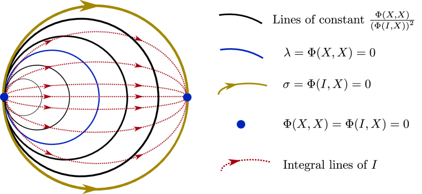
Figure 2: Dimensionally reduced depiction of $\mathbb{R}\textnormal{P}^{n+1}\setminus[I]$. The oriented lines indicate the fibres of the projection $\mathbb{R}\textnormal{P}^{n+1}\setminus[I]\to\mathbb{R}\textnormal{P}^{n}$; apart from those along the extended boundary at infinity – depicted here by a golden line – the fibres cross successive surfaces of constant growing $\frac{\Phi(X,X)}{(\Phi(I,X)^{2}}$ (ranging from $-\infty$ to $+\infty$).

3 Curved orbit decomposition

The object of this section is to study the curved picture of the previous homogenous model. Throughout, $\widetilde{M}$ is a compact manifold of dimension $n+1$ equipped with a projective structure $[\nabla]$. We assume that it is additionally endowed with a parallel non-degenerate tractor $H^{AB}$ of signature $(2,n)$ corresponding to a normal of the metrisability equation, and a nowhere vanishing parallel null-tractor $I^{A}$:

$$\nabla_{a}H^{AB} =0, \nabla_{a}I^{A} =0,$$ (3.1)

with $\det(H^{AB})\neq 0$ and $I^{A}I^{B}\Phi_{AB}=0$, where $\Phi_{AB}$ is the pointwise inverse of $H^{AB}$.

From Eq. (2.2), it is easily seen that in an arbitrary scale $\nabla$ the components of

$$I^{A}=n^{a}W_{a}^{A}+\rho X^{A},$$

satisfy the equations:

$$\nabla_{c}I^{A}=\left(\nabla_{c}n^{a}+\delta_{c}^{a}\rho\right)W_{a}^{A}+(\nabla_{c}\rho-P_{ca}n^{a})X^{A}=0\Leftrightarrow\begin{cases}\nabla_{c}n^{a}=-\delta_{c}^{a}\rho\\ \nabla_{c}\rho=P_{ca}n^{a} \end{cases}.$$ (3.2)

We emphasise that $n^{a}\in\Gamma(T\widetilde{M}(-1))$ is a scale-independent quantity whilst $\rho$ is not. On top of this vector field, we also have at our disposal two distinguished densities (of weight 1 and 2 respectively) that will be central to our development:

$$\sigma =\Phi_{AB}I^{A}X^{B},$$ (3.3)

$$\lambda =\Phi_{AB}X^{A}X^{B}.$$ (3.4)

These will allow us to state our main result concerning the curved orbits.

3.1 Resulting curved orbits

Theorem 3.1.

Let $\widetilde{M}$ be a $(n+1)$-dimensional closed manifold equipped with a projective structure $[\nabla]$, a non-degenerate parallel tractor $H^{AB}$ of signature $(2,n)$ and a nowhere vanishing parallel tractor $I^{A}$, such that $\Phi_{AB}I^{A}I^{B}=0$ where $\Phi_{AB}$ is the pointwise inverse of $H^{AB}$. Define, $n^{a}$, $\sigma$ and $\lambda$ by Eqs. (3.2)–(3.4).

1. The nowhere-vanishing null parallel tractor $I^{A}$ determines a first decomposition of $\widetilde{M}$ into two parts:

   $$\widetilde{M}=M\sqcup\mathcal{Z}(n),$$

   where $\mathcal{Z}(n):=\{x\in\widetilde{M},n^{a}=0\}$ is composed of finitely many isolated points and $M$ is the complement.

2. The additional data of the parallel tractor $H^{AB}$ then provides a further decomposition

   $$M=\mathcal{O}\sqcup\Sigma$$ (3.5)

   Here $\mathcal{O}$ is the open submanifold such that $\sigma\neq 0$ and (if non-empty) $\Sigma:=\mathcal{Z}(\sigma)\setminus\mathcal{Z}(n)$ is a smooth embedded hypersurface.

3. Finally, $\Sigma$ itself decomposes into further smooth submanifolds:

   $$\Sigma=\Sigma^{-}\sqcup\Sigma^{0}\sqcup\Sigma^{+}$$

   with $\Sigma^{-}:=\mathcal{Z}(\sigma)\cap\{\lambda<0\}$, $\Sigma^{+}:=\mathcal{Z}(\sigma)\cap\{\lambda>0\}$ and $\Sigma^{0}:=\mathcal{Z}(\sigma)\cap\mathcal{Z}(\lambda)\setminus\mathcal{Z}(n).$

Overall, in summary, we have:

$$M=\mathcal{O}\sqcup\Sigma^{-}\sqcup\Sigma^{0}\sqcup\Sigma^{+}\sqcup\mathcal{Z}(n).$$ (3.6)

It should be noted that $\widetilde{M}$ also admits another curved orbit decomposition relative to the data $(\lambda,H^{AB})$:

$$\widetilde{M}=U^{-}\sqcup\Lambda\sqcup U^{+},$$ (3.7)

where $U^{-}$, $\Lambda$ and $U^{-}$ are the sets $\{\lambda<0\}$, $\{\lambda=0\}$ and $\{\lambda>0\}$ respectively. In particular, it follows from [ČG14, ČGM14, FG18] that $\Lambda$ is the projective boundary of $U^{\pm}$. This would additionally lead to a further decomposition of $\mathcal{O}$ as $\mathcal{O}^{+}\sqcup\mathcal{O}^{0}\sqcup\mathcal{O}^{-}$, however, this will not be our central focus because the decomposition (3.7) is not preserved by the flow of the densified vector field $n^{a}$. Rather we have:

Theorem 3.2.

The flow of $n^{a}$ preserves the decomposition (3.6). Furthermore, the quotient $\mathcal{Q}_{\mathcal{O}}$ of $\mathcal{O}$ by this flow is a $n$-dimensional manifold.

If we assume that the quotient $\mathcal{Q}$ of $M=\widetilde{M}\setminus\mathcal{Z}(n)$ is a manifold we obtain the decomposition

generalising (2.12) in our curved setting.

Our present goal is to identify the geometric structures of each part and the relationships between them when they are all (save possibly $\mathcal{Z}(n)$) non-empty.

3.2 Derivation of Theorem 3.1

We recall that the Thomas $D$-operator is defined by the following equation in an arbitrary scale:

$$D_{A}T^{\mathscr{B}}=\nabla_{a}T^{\mathscr{B}}Z^{a}_{A}+wT^{\mathscr{B}}Y_{A}.$$ (3.8)

Where $T^{\mathscr{B}}$ is a section of an arbitrary bundle with tractor indices, of weight $w$; note that $D_{A}$ reduces weight by $1$. The following lemma will be useful:

Lemma 3.1.

Let $H^{AB},I^{A}$ be the parallel tractors (see Eq. (3.1)) introduced at the beginning of Section 3 and $\sigma,\lambda$ the densities defined by Eqs.(3.3) and (3.4), then:

$$I^{A}=H^{AB}D_{B}\sigma,$$ (3.9)

$$\Phi_{AB}X^{B}=\frac{1}{2}D_{A}\lambda,$$ (3.10)

$$\Phi_{AB}=\frac{1}{2}D_{A}D_{B}\lambda.$$ (3.11)

Proof.

In any scale, the identity tractor satisfies:

$$\delta^{A}_{B}=W^{A}_{a}Z_{B}^{b}\delta_{b}^{a}+X^{A}Y_{B}=D_{B}X^{A}.$$

Since the Thomas $D$ operator satisfies the Leibniz rule, we have:

$$D_{A}\sigma=D_{A}\Phi_{BC}I^{B}X^{C}+\Phi_{BC}D_{A}I^{B}X^{C}+\Phi_{BC}I^{B}D_{A}X^{C}$$

However, $\Phi$ and $I$ are weightless parallel tractors, so, by definition of the Thomas $D$ operator, $D_{A}\Phi_{BC}=0$ and $D_{A}I^{B}=0$. Thus:

$$D_{A}\sigma=\Phi_{BA}I^{B}.$$

Multiplying by $H^{AB}$ leads to the first equation.

In a similar fashion:

$$D_{A}\lambda=2\Phi_{BC}(D_{A}X^{B})X^{C}=2\Phi_{AC}X^{C}$$

Applying $D_{B}$ once more to this equation gives the last identity. ∎

We use this to prove the first elementary decomposition of the manifold $M$.

Proposition 3.1.

For any connection $\nabla$ in the projective class $\Sigma\cap\mathcal{Z}(\nabla_{c}\sigma)=\emptyset$. Consequently, when non-empty, $\Sigma$ is a smooth hypersurface of $M$.

Proof.

From (3.9), we see that on $\mathcal{Z}(\sigma)\cap\mathcal{Z}(\nabla_{c}\sigma)$ we must have:

$$0=D_{A}\sigma=\Phi_{AB}I^{B}.$$

Since by assumption, $\Phi_{AB}$ is non-degenerate this implies $I^{B}=0$ at such points. The result follows as we assume $I^{B}$ non-vanishing. ∎

The hypersurface $\Sigma$ will be interpreted as points at infinity of the region $\{\sigma\neq 0\}$; this is justified by:

Proposition 3.2.

Let $\mathcal{O}_{\pm}=\{\pm\sigma>0\}$, then the scale $\nabla^{\sigma}$ determined by $\sigma$ on $\mathcal{O}_{\pm}$ is projectively compact of order one and $\mathcal{O}_{\pm}\cup\Sigma$ is a projective compactification of $\mathcal{O}_{\pm}$.

Proof.

This is a direct consequence of [FG18, Proposition 2.4]. ∎

We recall from [ČG14, Proposition 2.3] that in this case the points are indeed “at infinity” with respect to the (parametrised) geodesics of $\nabla^{\sigma}$, they cannot be reached for a finite value of the affine parameter.

Whilst the decomposition of $\mathcal{O}$ associated with $H^{AB}$ and the density $\lambda$ studied in [FG18] is not of direct interest to us, the set $\mathcal{Z}(\sigma)\cap\mathcal{Z}(\lambda)$ is an important region. Ideally, we would like it to be a codimension $2$ submanifold of $\widetilde{M}$, the following proposition studies some possible singular points.

Proposition 3.3.

Recall that $I^{A}$ defines a weight $-1$ vector field $n^{a}=Z^{a}_{A}I^{A}$. The set of points $\mathcal{Z}(n)$, or equivalently points at which $I\propto X$, is composed of isolated points that lie in $\mathcal{Z}(\lambda)\cap\mathcal{Z}(\sigma)$. Since $\widetilde{M}$ is compact $\mathcal{Z}(n)$ is finite.

Proof.

We introduce an arbitrary scale $\nabla$, and recall that $I^{A}=\rho X^{A}+n^{a}Z_{a}^{A}$. Thus $n$ vanishes exactly at points where $I\propto X$.

Since $I$ is null, and by definition of $\sigma$, when $I\propto X$ it follows that we have both $\lambda=\Phi_{AB}X^{A}X^{B}\propto\Phi_{AB}I^{A}I^{B}=0$ and $\sigma=\Phi_{AB}X^{A}I^{B}\propto\Phi_{AB}X^{A}X^{B}=0.$ So $\mathcal{Z}(n)\subset\mathcal{Z}(\lambda)\cap\mathcal{Z}(\sigma)$. Let us prove that these are isolated points.

Using Eq. (2.2) we see that:

$$\nabla_{b}n^{a}=\nabla_{b}(I^{A}Z_{A}^{a})=-\delta_{b}^{a}Y_{A}I^{A}=-\delta_{b}^{a}\rho.$$

Since $I$ is nowhere vanishing, $\rho$ does not vanish on $\mathcal{Z}(n)$ and for any vector field $v^{b}$ that does not vanish on $\mathcal{Z}(n)$, we must have: $v^{b}\nabla_{b}n^{a}=\rho v^{b}\neq 0$ therefore $\mathcal{Z}(n)$ consists of isolated points. ∎

The following justifies the introduction of $\mathcal{Z}(n)$:

Proposition 3.4.

Let $\Sigma^{0}$ be the relative complement of $\mathcal{Z}(n)$ in $\mathcal{Z}(\sigma)\cap\mathcal{Z}(\lambda)$, then $\Sigma^{0}$ is a smooth submanifold of $M$ with codimension $2$.

Proof.

From Eqs. (3.9) and (3.10) one has $D_{A}\lambda=2\Phi_{AB}X^{B}$ and $D_{A}\sigma=\Phi_{AB}I^{B}$. When evaluated at points of $\mathcal{Z}(\sigma)\cap\mathcal{Z}(\lambda)$ these give

$$2\Phi_{AB}X^{B} =0\,Y_{A}+\nabla_{a}\lambda\,Z^{a}_{A} \Phi_{AB}I^{B} =0\,Y_{A}+\nabla_{a}\sigma\,Z^{a}_{A}.$$ (3.12)

To conclude the proof we need to show that there are no points of $\Sigma^{0}$ where $\nabla_{a}\lambda\propto\nabla_{a}\sigma$. However, at such points we would have for some density $f$:

$$2\Phi_{AB}X^{B}+f\Phi_{AB}I^{B}=0.$$ (3.13)

Since $\Phi_{AB}$ is invertible by hypothesis, this would mean $2X^{B}+fI^{B}=0$ which is excluded by definition of $\Sigma^{0}$. ∎

3.3 Derivation of Theorem 3.2

We will first need the following

Lemma 3.2.

In a generic scale $\nabla$, one has

$$n^{a}\nabla_{a}\sigma =-\rho\sigma$$ (3.14)

$$n^{a}\nabla_{a}\lambda =2\sigma-2\lambda\rho$$ (3.15)

Proof.

Since $I$ is null, it follows from Eq. (3.9) that: $I^{A}D_{A}\sigma=0$. In a generic scale $\nabla$ we have:

$$I^{A}=n^{a}W_{a}^{A}+\rho X^{A},\quad D_{A}\sigma=\sigma Y_{A}+\nabla_{a}\sigma Z^{a}_{A},$$

and therefore

$$I^{A}D_{A}\sigma=n^{a}\nabla_{a}\sigma+\rho\sigma=0.$$

Similarly from Eq. (3.10), and by definition of $\sigma$, we have:

$$2\sigma=I^{B}D_{B}\lambda=n^{a}\nabla_{a}\lambda+2\rho\lambda.$$

∎

The weight $-1$ vector field $n^{a}$ determines a distinguished family of unparametrised curves on $\widetilde{M}$. These are precisely the integral curves of any vector field $N^{a}$ obtained from $n^{a}$ by multiplying by a nowhere vanishing density $\nu$ of weight $1$ on $\widetilde{M}$; only the parametrisation depends on the choice of $\nu$. Since $\widetilde{M}$ is compact, any choice of $N^{a}$ leads to a complete vector field on $\widetilde{M}$ which restricts to a complete vector field on $M$. Lemma 3.2 shows that $n^{a}$ is tangent to the submanifolds $\Sigma$ and $\Sigma^{0}$ from which it follows immediately:

Corollary 3.1.

For any choice of nowhere vanishing density $\nu$ of weight $1$ on $\tilde{M}$, the action of $(\mathbb{R},+)$ given by the global flow of the vector field $N=\nu n$ on $N$, preserves the decomposition (3.6).

Definition 3.1.

Define $\mathcal{Q}$ to be the quotient space $M/\mathbb{R}$, equipped with the quotient topology, where the action of $\mathbb{R}$ is provided by the flow of any $N=\nu n$ and $\nu$ is a nowhere vanishing scale on $M$ that has a smooth extension to $\widetilde{M}$.

Let $\pi:M\rightarrow\mathcal{Q}$ be the natural projection, we define the distinguished open subset $\mathcal{Q}_{\mathcal{O}}=\pi(\mathcal{O})$ of $\mathcal{Q}$ ($\pi$ is an open map). Since $\mathcal{O}$ is stable under the action of $\mathbb{R}$ this can also be defined as the quotient space $\mathcal{O}/\mathbb{R}$ where the action of $\mathbb{R}$ is that of the flow of $N^{\sigma}=\sigma n$ equipped with the quotient topology.

We will now show that $\mathcal{Q}_{\mathcal{O}}$ has a natural manifold structure.

Theorem 3.3.

Let $\pi:\mathcal{O}\rightarrow\mathcal{Q}_{\mathcal{O}}$ be the canonical projection. Then there is a unique smooth structure on $\mathcal{Q}_{\mathcal{O}}$ such that $\pi$ has the structure of a (right) $\mathbb{R}$-principal fibre bundle. The zero set of the function $l:=\sigma^{-2}\lambda:\mathcal{O}\to\mathbb{R}$ defines a global section and yields a preferred global diffeomorphism

$$\begin{array}[]{ccc}\mathcal{O}&\simeq&\mathbb{R}\times\mathcal{Q}_{\mathcal{O}}\\ x&\mapsto&(\frac{1}{2}l(x),\pi(x))\end{array}.$$

In particular, $\omega_{a}=\frac{1}{2}\nabla_{a}l$ is a canonical principal connection.

Proof of Theorem 3.3.

We apply the characterisation of principle fibre bundles [Sha97, Theorem 4.2.4]. It suffices to show that action is free and proper. We shall work in the distinguished scale determined by $\sigma$ on $\mathcal{O}$. We define $l=\sigma^{-2}\lambda$, and let $\gamma$ denote an arbitrary integral curve of $N=\sigma n$, then Eq. (4.5) leads to:

$$\frac{\textnormal{d}}{\textnormal{d}t}\lambda(\gamma(t))=(N^{a}\nabla_{a}l)|_{\gamma(t)}=2.$$ (3.16)

It follows that $l=2t+l_{0}$ along the curve $N$, consequently $l$ is strictly monotonous and unbounded along such a curve. Thus the action is:

• free: the isotropy subgroup of any point $x$ is either $\mathbb{R}$ (i.e. $\forall t \in\mathbb{R},\phi^{N}_{t}(x)=x$) or $T\mathbb{Z}$ for some $T\in\mathbb{R}$. The first case is excluded as $n^{a}$ does not vanish on $\mathcal{O}$. If it was of the form $T\mathbb{Z}$ with $T>0$ then the curve $t\mapsto\phi^{N}_{t}(x)$ would be periodic, but this is excluded because $l$ is strictly monotonous along such a curve. Hence, $T=0$.

• proper: Let $K$ be a compact subset of $M\setminus\Sigma$, then, $l$, being continuous, is bounded above and below on $K$ say: $\forall x\in K,m\leq l(x)\leq M$. Let $x\in K$, then:

  $$l(\phi^{N}_{t}(x))=2t+l(x)\geq 2t+m.$$

  So for any $x\in K$, when $t\geq(\frac{M-m+1}{2})$ $\phi^{N}_{t}(x)$ has definitively left $K$. This implies that $\{t\in\mathbb{R},tK\cap K\neq\emptyset\}$ is compact.

Finally, Eq. (3.16) implies that $\frac{1}{2}l(\phi^{N}_{t}(p))=\frac{1}{2}l(p)+t$, which shows that $\frac{1}{2}l$ provides a canonical trivialisation of $\mathcal{O}$. ∎

Remark 3.1.

For future computations it will be useful to note that $N$ is by definition a fundamental vector field on $\mathcal{O}$. Recall that if $P$ is a principal $G$ bundle then the fundamental vector fields $X^{*}$ associated with $X\in\mathfrak{g}$ is defined at $p\in P$ by

$$A^{*}_{p}=\left.\frac{\textnormal{d}}{\textnormal{d}t}(p\exp(Xt))\right|_{t=0},$$

in the simple case we consider of the abelian Lie algebra $\mathbb{R}$, the exponential map satisfies $\exp(1t)=t$ therefore:

$$1^{*}_{x}=\left.\frac{\textnormal{d}}{\textnormal{d}t}(p\cdot t)\right|_{t=0}=\left.\frac{\textnormal{d}}{\textnormal{d}t}\phi^{N}_{t}(x)\right|_{t=0}=N_{x}.$$

It is not clear that $\mathcal{Q}$ itself can be equipped with a smooth structure, as the behaviour of $n$ near $\Sigma$ (to which it is tangent) is unclear. However, to simplify our discussion we shall make the assumption that $\mathcal{Q}$ can be equipped with a smooth structure such that $\pi:M\rightarrow\mathcal{Q}$ is a fibre bundle with fibre $\mathbb{R}$.

We conclude this section by recording the following useful result.

Lemma 3.3.

Let $\nu$ be any nowhere vanishing scale and $N^{a}=\nu n^{a}$, $g^{ab}=\nu^{2}\zeta^{ab}$ then

$$\mathcal{L}_{N}g^{ab}=2N^{(a}\lambda^{b)}+2\rho g^{ab},$$ (3.17)

where $\lambda^{a}$ and $\rho$ are respectively defined by equations (2.6) and (3.2).

Proof.

For any vector field $X$, we have the identity

$$\mathcal{L}_{X}g^{ab}=\nabla_{X}g^{ab}-2\nabla_{c}X^{(a}g^{b)c}.$$

Taking $X^{a}=N^{a}$ and making use of (2.6) and (3.2) one obtains

$$\mathcal{L}_{N}g^{ab}=2N^{(a}\lambda^{b)}+2\rho g^{ab}.$$ (3.18)

∎

4 Geometry of the open orbit $\mathcal{O}$

In this section we restrict ourselves to the curved orbit $\mathcal{O}$ on which $\sigma$ is nowhere vanishing. We can therefore form the undensitised bi-vector, vector field and function

$$g^{ab} =\sigma^{2}\zeta^{ab}, N^{a} =\sigma n^{a} l =\sigma^{-2}\lambda.$$ (4.1)

The scale $\nabla$ determined by $\sigma$ (i.e. such that $\nabla\sigma=0$) has the following important properties:

Lemma 4.1.

In the scale $\nabla$ determined by $\nabla\sigma=0$, we have:

$$\nabla_{c}n^{a} =-\delta^{a}_{c}\rho=0,$$ (4.2)

$$\lambda n^{a} =-\frac{1}{2}\sigma\zeta^{ab}\nabla_{b}\lambda,$$ (4.3)

$$\nabla_{c}\zeta^{ab} =-2\sigma^{-1}\delta^{(a}_{c}n^{b)}.$$ (4.4)

Proof.

Equations (4.2) follows from Eqs. (3.2), (3.9), $I^{2}=0$ and the definition of the scale:

$$\rho=I^{A}Y_{A}=I^{A}(\sigma^{-1}D_{A}\sigma)=\sigma^{-1}I^{2}=0.$$

To prove the second relation $\eqref{sigma scale => n=grad(l)}$ we remark that from Eq. (3.10) one has: $X^{A}=\frac{1}{2}H^{AB}D_{B}\lambda$. Contracting with $Z_{A}^{a}$ then gives

$$0=\frac{1}{2}Z_{A}^{a}H^{AB}D_{B}\lambda=\frac{1}{2}\zeta^{ab}\nabla_{b}\lambda+Z_{A}^{a}\underbrace{H^{AB}Y_{B}}_{\sigma^{-1}H^{AB}D_{B}\sigma}\lambda=\frac{1}{2}\zeta^{ab}\nabla_{b}\lambda+\sigma^{-1}n^{a}\lambda,$$

where we have used Eq. (3.9). Finally, the last relation $\eqref{sigma scale => lambda^a =n^a}$ comes from:

$$\nabla_{c}\zeta^{ab}=\nabla_{c}Z_{A}^{a}H^{AB}Z_{B}^{b}=-\delta^{a}_{c}Y_{A}H^{AB}Z_{B}^{b}-\delta^{b}_{c}Z_{B}^{b}H^{AB}Y_{B}=-2\sigma^{-1}\delta^{(a}_{c}n^{b)}.$$

∎

Remark 4.1.

Since $\sigma$ is covariantly constant for the connection $\nabla$, Eqs. (4.2),(4.3), and (4.4) translate directly in terms of the quantities $g,N,f$:

$$\nabla_{c}N^{a}=0,\quad N^{a}=-\frac{1}{2}l^{-1}g^{ab}\nabla_{b}l,\quad\nabla_{c}g^{ab}=-2\delta_{c}^{(a}N^{b)}.$$

Equation (4.2) means that the integral lines of $N^{a}$ are geodesically parametrised for $\nabla$. In fact, combining this with Lemma 3.2, one sees that

$$N^{a}\nabla_{a}l=2$$ (4.5)

in other terms $l$ coincides with this parametrisation. This however fails to be a gradient flow for $g^{ab}$: Eq. (4.3) recovers that $g^{ab}$ is degenerate along $l=0$, and one rather has $N^{a}=-\frac{1}{2}g^{ab}(l^{-1}\nabla_{b}l)$. The last identity (4.4) is crucial to derive the following canonical form:

Proposition 4.1.

$$g^{ab}=-lN^{a}N^{b}+\tilde{h}^{ab}$$ (4.6)

where $\tilde{h}^{ab}\nabla_{b}l=0$ and $\mathcal{L}_{N}\tilde{h}^{ab}=0$.

Proof.

We recall from Lemma 3.3 that in a generic scale $\nu$

$$\mathcal{L}_{N}g^{ab}=2N^{(a}\lambda^{b)}+2\rho g^{ab},$$ (4.7)

where $\lambda^{a}$ is defined by the relation $\nabla_{c}\zeta^{ab}-2\delta^{(a}_{c}\lambda^{b)}=0$. When evaluated in the scale $\sigma$ this becomes, by making use of (4.2) and (4.4),

$$\mathcal{L}_{N}g^{ab}=-2N^{a}N^{b}.$$ (4.8)

Since $N^{a}\nabla_{a}l=2$, this is equivalent to $\mathcal{L}_{N}(g^{ab}+lN^{a}N^{b})=0$ and therefore one can write

$$g^{ab}=-lN^{a}N^{b}+\tilde{h}^{ab}$$ (4.9)

with $\mathcal{L}_{N}\tilde{h}^{ab}=0$. We conclude by computing $\tilde{h}^{ab}\nabla_{b}l$

$$\tilde{h}^{ab}\nabla_{b}l =g^{ab}\nabla_{b}l+lN^{a}N^{b}\nabla_{b}l$$ (4.10)

$$=-2lN^{a}+2lN^{a}=0$$ (4.11)

where we made use of (4.3). ∎

Using Lemma 4.1 we have:

Proposition 4.2.

At points of $\mathcal{O}$ where $g^{ab}$ is invertible, the corresponding metric is Ricci-flat.

Remark 4.2.

Note that the Ricci flat metric $\sigma^{2}\zeta^{ab}$ of this proposition differs from the Einstein metric with a non-vanishing scalar curvature $\lambda\zeta^{ab}$ that is given by the projective compactification of order 2 as in [ČGM14].

Proof.

Calculating in the scale $\nabla$,

$$0=D_{B}I^{A}=D_{B}(H^{AC}D_{C}\sigma)=H^{AC}D_{B}(\sigma Y_{C}),$$

since $H^{AB}$ is non-degenerate we conclude that $D_{B}(\sigma Y_{C})=0$, therefore,

$$0=D_{B}(\sigma Y_{C})=(D_{B}\sigma)Y_{C}+\sigma(D_{B}Y_{C})=\sigma P_{bc}Z^{b}_{B}Z^{c}_{C},$$

hence, on $\mathcal{O}$, $P_{bc}=0$.

Define, when $l\neq 0$, a torsion-free connection $\tilde{\nabla}$ by:

$$\tilde{\nabla}_{c}\xi^{b}=\nabla_{c}\xi^{b}+N^{b}g_{cd}\xi^{d},$$ (4.12)

for any vector field $\xi^{b}$.

Remark 4.3.

Note that this is not a projective change of connection.

It is straightforward to check that $\tilde{\nabla}$ is the Levi-Civita connection of $g$. Let us calculate the Ricci tensor $\tilde{R}_{ab}$ of $\tilde{\nabla}$ with respect to that of $\nabla$ which we denote by $R_{ab}$. In fact, $R_{ab}$ vanishes since $\sigma$ is a special scale and $R_{ab}=(n-1)P_{ab}=0$. We have:

$$\tilde{R}_{ab}=\underbrace{R_{ab}}_{=0}+\underbrace{N^{c}\nabla_{c}g_{ab}}_{\frac{1}{2}\Upsilon_{a}\Upsilon_{b}}+\frac{1}{2}\nabla_{a}\Upsilon_{b}-\frac{1}{4}\Upsilon_{a}\Upsilon_{b}-\frac{1}{2}\underbrace{(N^{c}\Upsilon_{c})}_{2\sigma^{2}\lambda^{-1}}g_{ab}$$ (4.13)

Thus:

$$\tilde{R}_{ab}=\frac{1}{2}\nabla_{a}\Upsilon_{b}+\frac{1}{4}\Upsilon_{a}\Upsilon_{b}-\sigma^{2}\lambda^{-1}g_{ab}$$ (4.14)

where we have introduced: $\Upsilon=\lambda^{-1}\nabla\lambda$. Using $H^{AB}\Phi_{BC}=\delta^{A}_{C}$ and Equation (3.11) one finds that:

$$\lambda^{-1}\sigma^{2}g_{ab}=\frac{1}{2}\left(\lambda^{-1}\nabla_{a}\nabla_{b}\lambda-\frac{1}{2}\lambda^{-2}\nabla_{a}\lambda\nabla_{b}\lambda\right)=\frac{1}{2}\left(\nabla_{a}\Upsilon_{b}+\frac{1}{2}\Upsilon_{a}\Upsilon_{b}\right),$$

which shows that:

$$\tilde{R}_{ab}=0.$$

∎

Proposition 4.1 suggests that $\tilde{h}^{ab}$ might induce a smooth tensor on the quotient $\mathcal{Q}_{\mathcal{O}}$ of $\mathcal{O}$ by the integral lines of $N^{a}$. In turn, Eqs (4.4) and (4.12) suggest that the connection $\nabla$ factors to the quotient and this factorisation will yield the Levi-Civita connection of such a tensor field; the following results confirm this intuition.

Proposition 4.3.

$g^{ab}$ induces a bilinear form $h^{ab}$ on $\mathcal{Q}_{\mathcal{O}}$ which is everywhere non-degenerate.

Proof.

Let $\alpha,\beta$ be $1$-form fields on $\mathcal{Q}_{\mathcal{O}}$ and consider the smooth function on $\mathcal{O}$ defined by $g(\pi^{*}\alpha,\pi^{*}\beta)$, Lemma 4.1 implies that $g(\pi^{*}\alpha,\pi^{*}\beta)=\tilde{h}(\pi^{*}\alpha,\pi^{*}\beta)$ is constant on the fibres of $\mathcal{O}\to\mathcal{Q}_{\mathcal{O}}$ and so factorises to a well-defined smooth map on $\mathcal{Q}_{\mathcal{O}}$, that we denote by $h(\alpha,\beta)$. It is clearly symmetric and tensorial so determines a bilinear form on $T^{*}\mathcal{Q}_{\mathcal{O}}$.

Now $\zeta^{ab}$ is degenerate exactly at points where $\lambda=0$ and so $g^{ab}=\sigma^{2}\zeta^{ab}$ is invertible at any point where $l=\sigma^{-2}\lambda\neq 0$. However, at any point of $\mathcal{O}$, one has the decomposition $T^{*}\mathcal{O}=\text{Span}(\nabla_{a}l)\oplus\pi^{*}(T^{*}\mathcal{Q}_{\mathcal{O}})$ and by Lemma 4.1 the corresponding decomposition of $g^{ab}$ is $\text{diag}(-l,h^{ab})$. Therefore $g^{ab}$ can only be invertible at points where $l\neq 0$ if $h^{ab}$ is. ∎

Proposition 4.4.

The connection $\nabla$ is invariant under the flow of $N$.

Proof.

First we consider instead the principal connection $\alpha$ determined by $\nabla$ on the frame bundle $P^{1}(\mathcal{O})$. The $1$-parameter group of diffeomorphisms generated by $N$ induces a $1$-parameter group of diffeomorphisms on $P^{1}(\mathcal{O})$. Since $N$ is parallel, the infinitesimal generator $\tilde{N}$ of the induced $1$-parameter group of diffeomorphisms is precisely the horizontal lift of $N$ with respect to the principal connection $\alpha$. This can be seen, for instance, by a swift computation in a canonical coordinate system of $P^{1}(\mathcal{O})$. Since the Lie derivative satisfies the Leibniz rule we have:

$$(\mathcal{L}_{\tilde{N}}\alpha)(\tilde{X})=\tilde{N}(\alpha(\tilde{X}))-\alpha([\tilde{N},\tilde{X}]).$$

If $\tilde{X}=X^{*},X\in\mathfrak{gl}(n+1,\mathbb{R})$ is a fundamental vector field, this vanishes entirely; indeed: $\alpha(X^{*})=X$ is constant and the Lie bracket between a fundamental field and a horizontal vector field vanishes. Hence, $\mathcal{L}_{\tilde{N}}\alpha$ is a horizontal and equivariant $\mathfrak{gl}(n+1,\mathbb{R})$ valued 1-form. In fact, restricting to the case where $\tilde{X}$ is horizontal ($\alpha(\tilde{X})=0$), we see that it reduces to

$$(\mathcal{L}_{\tilde{N}}\alpha)(\tilde{X})=-\alpha([\tilde{N},\tilde{X}])=\Omega(\tilde{N},\tilde{X}),$$

where $\Omega$ is the curvature $2$-form. It follows that we should compute: $N^{a}R_{ab\phantom{c}d}^{\phantom{ab}c}.$

Using Lemma 4.1, we see that although $\nabla$ is not the Levi-Civita connection of $g$, it does satisfy: $\nabla_{d}\nabla_{c}g^{ab}=0,$ which leads to the following symmetry of the curvature tensor:

$$R^{abcd}=-R^{abdc},$$

where all indices are raised with $g^{ab}$. This implies that $R^{abcd}$ has all the symmetries of the curvature tensor of the Levi-Civita connection of a metric. In particular, at points where $l\neq 0$,

$$N^{a}R_{a}^{\phantom{a}bcd}=-\frac{1}{2}l^{-1}\nabla_{a}lR^{abcd}=\frac{1}{2}l^{-1}\nabla_{a}lR^{cdba}=-R^{cdb}_{\phantom{cdb}a}N^{a}.$$

However, since $N^{a}$ is parallel, we must have: $R_{ab\phantom{c}d}^{\phantom{ab}c}N^{d}=0$, thus at points where $l\neq 0$ (at which $g^{ab}$ is non-degenerate):

$$N^{a}R_{ab\phantom{c}d}^{\phantom{ab}c}=0,$$

but these points are dense in $\mathcal{O}$, so the above identity extends to $\mathcal{O}$ by continuity. Consequently:

$$\mathcal{L}_{\tilde{N}}\alpha=0.$$

∎

Before we state the immediate corollary, we first record a consequence of the final steps of our computation:

Lemma 4.2.

At every point of $M$:

$$n^{a}W_{ab\phantom{c}d}^{\phantom{ab}c}=0$$

Proof.

Both the Weyl tensor $W_{ab\phantom{c}d}^{\phantom{ab}c}$ and $n^{a}$ are projectively invariant, hence this is a projectively invariant statement and it suffices to check in one particular scale. On $\mathcal{O}$, $\sigma$ is a scale and we have seen above that the Riemann tensor of the connection $\nabla^{\sigma}$ satisfies:

$$N^{a}R_{ab\phantom{c}d}^{\phantom{ab}c}=\sigma n^{a}R_{ab\phantom{c}d}^{\phantom{ab}c}=0,$$

therefore $n^{a}R_{ab\phantom{c}d}^{\phantom{ab}c}=0$ where $\sigma\neq 0$. However, we saw in the proof of Proposition 4.2 that $P_{bc}=0$ in this special scale, i.e. $\beta_{ab}=0$ too. Hence: $R_{ab\phantom{c}d}^{\phantom{ab}c}=W_{ab\phantom{c}d}^{\phantom{ab}c}$ and thus the result holds on $\mathcal{O}$, since $\mathcal{O}$ is dense in $M$ it extends to $M$ by continuity. ∎

The immediate corollary of Proposition 4.4 is that :

Corollary 4.1.

$\nabla$ induces a torsion-free connection $\bar{\nabla}$ on the quotient $\mathcal{Q}_{\mathcal{O}}$.

Proof.

Let $\bar{X},\bar{Y}$ be vector fields on $\mathcal{Q}_{\mathcal{O}}$, and $X,Y$ their horizontal lifts to vector fields $\mathcal{O}$ using the principal connection $\omega$ in Theorem 3.3 and define:

$$\bar{\nabla}_{X}Y=\pi_{*}(\nabla_{\overline{X}}\overline{Y})$$

By the previous proposition, this is independent of choice on the fibre and so is a well-defined vector field on $Q$. This is clearly linear in $X$ and satisfies the Leibniz rule in $Y$ and therefore is a connection. It is torsion-free as:

$$\bar{\nabla}_{\bar{Y}}{\bar{X}}-\bar{\nabla}_{\bar{X}}{\bar{Y}}=\pi_{*}(\nabla_{X}Y-\nabla_{Y}X)=\pi_{*}([X,Y])=[\pi_{*}(X),\pi_{*}(Y)]=[\bar{X},\bar{Y}],$$

by naturality of the pushforward. ∎

Proposition 4.5.

The induced connection $\bar{\nabla}$ on $\mathcal{Q}_{\mathcal{O}}$ is the Levi-Civita connection of the form $h$ defined in Proposition 4.3; furthermore the Lorentzian geometry $(Q,h_{ab})$ is Ricci-flat.

Proof.

If $\bar{X}$ is a vector field on $\mathcal{Q}_{\mathcal{O}}$, $X$ its horizontal lift to a vector field on $\mathcal{O}$, and $\alpha,\beta$ are 1-forms on $\mathcal{Q}_{\mathcal{O}}$, then at every point $x\in\mathcal{O}$ we have:

$$\begin{aligned} (\bar{\nabla}_{\bar{X}}h)(\alpha,\beta)(\pi(x))&=\nabla_{\bar{X}}g(\pi^{*}\alpha,\pi^{*}\beta)(x)\\ &=-(\pi^{*}\alpha)(N)(\pi^{*}\beta)(X)(x)-(\pi^{*}\beta)(N)(\pi^{*}\alpha)(X)\\ &=0.\end{aligned}$$

This shows that $\bar{\nabla}$ is the Levi-Civita connection for $h$.

Now, if $\bar{X},\bar{Y}$ and $\bar{Z}$ are vector fields on $\mathcal{Q}_{\mathcal{O}}$ and $X,Y,Z$ their horizontal lifts to $\mathcal{O}$ then, noting that $\nabla_{a}l[X,Y]^{a}=0$, and using that $N$ is parallel for $\nabla$, we have:

$$\bar{R}(\bar{X},\bar{Y})\bar{Z}=\pi_{*}(R(X,Y)Z).$$

If $(\bar{E}_{i})$ is an arbitrary local frame of $T\mathcal{Q}_{\mathcal{O}}$ then lifting them horizontally to fields on $\mathcal{O}$, we obtain a local frame $(E_{i},N)$ of $TM$, with dual frame: $(\omega^{i},\frac{1}{2}\textnormal{d}l)$. Now:

$$\textrm{Ric}(Y,Z)=\sum_{i}\omega^{i}(R(E_{i},Y)Z)+\frac{1}{2}\textnormal{d}l(R(N,Y)Z)=\sum_{i}\omega^{i}(R(E_{i},Y)Z).$$

By definition, $\omega^{i}(E_{j})=\delta^{i}_{j}$, $\omega^{i}(N)=0$ therefore: $\mathcal{L}_{N}\omega^{i}(E_{j})=-\omega^{i}([N,E_{j}])=0$. Thus, the $\omega^{i}$ are the pullbacks of a local frame $\bar{\omega}^{i}$ of $\mathcal{Q}_{\mathcal{O}}$ and it follows that:

$$0=\textrm{Ric}(Y,Z)=\overline{\textrm{Ric}}(\tilde{Y},\tilde{Z}).$$

We can also check this in terms of the global trivialisation given in Theorem 3.3:

$$\begin{array}[]{ccc}T\mathcal{O}&\to&\text{Span}(N)\oplus T\mathcal{Q}_{\mathcal{O}}\\ v^{a}&\mapsto&(\frac{1}{2}(v^{b}dl_{b})N^{a},v^{b}\nabla_{b}x^{\mu})\end{array}$$ (4.15)

the decomposition of the tangent bundle given by $l$. At any point where $\lambda\neq 0$ the inverse of $g^{ab}$ is, in this decomposition,

$$g_{ab}=\begin{pmatrix}-\frac{1}{l}&0\\ 0&h_{\mu\nu}\end{pmatrix}.$$ (4.16)

The local connection form of the Levi-Civita connection in coordinates $(x^{0}=\frac{1}{2}l,x^{\mu})$ adapted the global trivialisation is then given by

$$(\omega^{i}_{\,j})_{c}=\nabla_{c}x^{0}\begin{pmatrix}-\frac{1}{2l}&0\\ 0&0\end{pmatrix}+\nabla_{c}x^{\rho}\begin{pmatrix}0&0\\ 0&\gamma^{\mu}_{\rho\nu}\end{pmatrix}$$ (4.17)

where $\gamma^{\mu}_{\rho\nu}$ are the Christoffel symbols of the Levi-Civita connection of $h$. The local curvature form is

$$(F^{i}{}_{j})_{cd}=\nabla_{c}x^{\rho}\wedge\nabla_{d}x^{\sigma}\begin{pmatrix}0&0\\ 0&R^{\mu}{}_{\nu\rho\sigma}\end{pmatrix}$$ (4.18)

where $R^{\mu}{}_{\nu\rho\sigma}$ is the Riemann tensor of $h$. Since by Proposition 4.2 $g_{ab}$ is Ricci-flat it immediately follows that $h_{ab}$ is also. ∎

5 Geometry of $\mathcal{Q}$

We recall that $M:=\widetilde{M}\setminus\mathcal{Z}(n)$ and assume, as in Theorem 3.2, that its quotient $\mathcal{Q}$ by the flow of $n^{a}$ can be equipped with a smooth manifold structure. It then decomposes as

$$\mathcal{Q}=\mathcal{Q}_{\mathcal{O}}\cup\mathcal{H}^{-}\cup\mathcal{H}^{0}\cup\mathcal{H}^{+}.$$ (5.1)

From the previous section, in particular Proposition 4.3 and Proposition 4.5, we learned that $\mathcal{Q}_{\mathcal{O}}$ is equipped with a Ricci flat Lorentzian metric. We will now show that this metric is projectively compact of order 1 with $\mathcal{H}^{-}\cup\mathcal{H}^{0}\cup\mathcal{H}^{+}$ forming the projective boundary.

In order to prove this we will proceed in 3 steps. First, we will discuss how to identify densities and tractor bundles on $Q$ with subbundles of bundles on $M$ via pullback. This first step can be thought as an infinitesimal version of the relations between the homogeneous models as in Figure 1. In particular, since $H^{AB}$ and $I_{A}$ are covariantly constant on the whole of $M$ they will define corresponding tractor fields $\bar{H}^{AB}$ and $\bar{I}_{A}$ on $\mathcal{Q}$. As a result of the quotient by $I^{A}$ which is necessary for the identification, $\bar{H}^{AB}$ then is degenerate of kernel $\bar{I}_{A}$. Secondly, we will show that the projective tractor connection $\nabla$ of $M$ induces a normal projective tractor connection $\bar{\nabla}$ on $\mathcal{Q}$ and that $\bar{\nabla}_{c}\bar{H}^{AB}=0$, $\bar{\nabla}_{c}\bar{I}_{A}=0$. This will imply by [ČG14, FG18] that $\mathcal{Q}$ is equipped with a Ricci flat metric projectively compact of order 1. Finally we will show that on $\mathcal{Q}_{\mathcal{O}}$ this metric coincides with the Ricci flat metric resulting from the previous section.

5.1 Densities and tractors of $\mathcal{Q}$

We will first show how to relate densities on $M$ with densities on $\mathcal{Q}$. Extending this at the level of $1$-jets will yield the corresponding identification between projective tractors $\mathcal{T}_{M}$ on $M$ with projective tractors $\mathcal{T}_{\mathcal{Q}}$ of $\mathcal{Q}$.

5.1.1 Densities on $\mathcal{Q}$

In the sequel, we shall assume that the flow of $n^{a}\in\Gamma\left(TM(-1)\right)$ on $M:=\widetilde{M}\setminus\mathcal{Z}(n)$ defines a fibre bundle

$$\pi:\begin{array}[]{ccc}M&\longrightarrow&\mathcal{Q}\end{array}$$ (5.2)

with fibres given by the integral lines, and general fibre $\mathbb{R}$.

Let $\mathcal{E}_{M}(w)$ and $\mathcal{E}_{\mathcal{Q}}(w)$ be projective densities of $M$ and $\mathcal{Q}$ respectively.

Proposition 5.1.

There is a canonical isomorphism

$$\pi^{*}\mathcal{E}_{\mathcal{Q}}(w)\simeq\mathcal{E}_{M}(w).$$ (5.3)

Proof.

By definition of projective densities (see Section 2.1), the bundle $\mathcal{E}_{M}(w)$ is canonically isomorphic to $\big{(}\textnormal{Vol}(M)\big{)}^{-\frac{w}{n+2}}$ where $\textnormal{Vol}(M)=\big{(}\Lambda^{n+1}T^{*}M\otimes\Lambda^{n+1}T^{*}M\big{)}^{\frac{1}{2}}$ is the bundle of volume densities of $M$.

Therefore, there always exists a canonical nowhere vanishing section $\varepsilon^{2}_{a_{1}\dots a_{n+1},b_{1}\dots b_{n+1}}$ of $[(\Lambda^{n+1}T^{*}M)\otimes(\Lambda^{n+1}T^{*}M)](2(n+2))$ realising the canonical isomorphism

$$\varepsilon^{2}_{a_{1}\dots a_{n+1},b_{1}\dots b_{n+1}}:\begin{array}[]{ccc}\mathcal{E}_{M}(-2(n+2))&\simeq&\Lambda^{n+1}T^{*}M\otimes\Lambda^{n+1}T^{*}M\end{array}$$ (5.4)

We will note $TM/n$ the fibre bundle over $M=\widetilde{M}\setminus\mathcal{Z}(n)$ obtained by taking the point-wise quotient of $TM$ by the span of $sn^{a}$ where $s$ is any “true scale”, i.e. nowhere vanishing density of weight $1$; the quotient is independent of the choice of $s$. By construction, the annihilator $\mathcal{N}^{*}$ of $n^{a}$ in $T^{*}M$ is identified with $(TM/n)^{*}$ as well as with the pull-back bundle $\pi^{*}(T^{*}Q)$. It follows that:

$$\nu_{a_{1}\dots a_{n},b_{1}\dots b_{n}}:=\varepsilon^{2}_{aa_{1}\dots a_{n},bb_{1}\dots b_{n}}n^{a}n^{b},$$ (5.5)

is identified with a nowhere vanishing section of $\pi^{*}\big{(}\Lambda^{n}T^{*}Q\otimes\Lambda^{n}T^{*}Q\big{)}\otimes\mathcal{E}_{M}\big{(}2(n+1)\big{)}$ and thus realises an isomorphism

$$\mathcal{E}_{M}\big{(}-2(n+1)\big{)}\simeq\pi^{*}\big{(}\Lambda^{n}T^{*}Q\otimes\Lambda^{n}T^{*}Q\big{)}\simeq\pi^{*}\mathcal{E}_{\mathcal{Q}}(-2(n+1)).$$ (5.6)

Taking roots yields the desired isomorphism for arbitrary weights $w$.∎

This identification enables us to construct a natural differential operator on projective densities of $M$. Indeed, the action of the Lie derivative on $\pi^{*}\big{(}\Lambda^{n}T^{*}Q\otimes\Lambda^{n}T^{*}Q\big{)}$ along $n^{a}$ induces a differential operator $D_{n}$ on $\mathcal{E}_{M}(w)$ by closing the following commutative diagram:

Figure 3: Defining diagram of $D_{n}$

Proposition 5.2.

The maps appearing in the commutative diagram in Figure 3 are well defined linear differential operators of order $1$. In a given projective scale, we have

$$\begin{array}[]{cccc}D_{n}:&\mathcal{E}_{M}(w)&\longrightarrow&\mathcal{E}_{M}(w-1)\\ &\tau&\longmapsto&(\nabla_{n}+w\rho)\tau\end{array}$$ (5.7)

where $\rho:=-\tfrac{1}{n+1}\nabla_{a}n^{a}=Y_{A}I^{A}.$

Proof.

Let $s$ be an arbitrary non-vanishing density of weight $1$ on $M$, and $X^{a}=sn^{a}$. Since $\pi^{*}(\Lambda^{n}T^{*}Q)$ can be identified with $n$-forms on $M$ that vanish whenever at least one of its arguments is a vertical vector, we can apply the Lie derivative in the usual sense. Let $\nabla$ be the scale determined by $s$ in the projective class then for any $\alpha\in\pi^{*}(\Lambda^{n}T^{*}Q)$:

$$\mathcal{L}_{X}\alpha=X\lrcorner\textnormal{d}\alpha=\nabla_{X}\alpha-ns\rho\alpha=s(n^{a}\nabla_{a}\alpha-n\rho\alpha),$$

where we recall $\nabla_{b}n^{a}=-\rho\delta_{b}^{a}$. Since this is proportional to the scale $s$, we see that this yields a well-defined linear operator $\mathcal{L}_{n}:\pi^{*}(\Lambda^{n}T^{*}Q)\to\pi^{*}(\Lambda^{n}T^{*}Q)(-1)$. According to the commutative diagram in Figure 3, to define $D_{n}$ on densities of weight $-2(n+1)$, we must set:

$$D_{n}\tau=\nu^{-1}\mathcal{L}_{n}(\nu\tau) =\nu^{-1}\left(\nabla_{n}(\nu\tau)-2n\rho\nu\tau\right)$$

$$=\nu^{-1}\left(\nu\nabla_{n}\tau-2\rho\nu\tau-2n\rho\nu\tau\right)$$

$$=\nabla_{n}\tau-2(n+1)\rho\tau.$$

where $\nu$ is a short-hand notation for the section (5.5). Eq. (5.7) follows for densities of arbitrary weight $w$. ∎

Proposition 5.1 allows us to identify projective densities $\mathcal{E}_{M}(w)$ on $M$ with pullbacks of densities on $\mathcal{Q}$. Since sections $\tau$ of $\pi^{*}\mathcal{E}_{\mathcal{Q}}(w)$ which are the pullback $\tau=\pi^{*}\bar{\tau}$ of sections of $\mathcal{E}_{\mathcal{Q}}(w)$ are precisely those with vanishing Lie derivative in the direction $n^{a}$ we obtain, from the commutative diagram 3, the following characterisation of densities on $Q$:

Proposition 5.3.

Densities $\bar{\tau}$ of weight $w$ on $\mathcal{Q}$ are canonically identified with densities (of weight $w$) $\tau$ on $M$ satisfying $D_{n}\tau=0$:

$$D_{n}\tau =0,\quad\tau\in\Gamma(\mathcal{E}_{M}(w)) \Leftrightarrow \tau =\pi^{*}\bar{\tau},\qquad\bar{\tau}\in\Gamma(\mathcal{E}_{\mathcal{Q}}(w)).$$ (5.8)

In the righthand side of the above equivalence, and throughout the following sections of this article, we abuse notation and use the isomorphism (5.3) to identify sections of $\mathcal{E}_{M}(w)$ and $\pi_{*}\left(\mathcal{E}_{\mathcal{Q}}(w)\right)$, i.e. we will think of $\pi^{*}\bar{\tau}$ as a section of $\mathcal{E}_{M}(w)$.

Remark 5.1.

This shows that when $\mathcal{Q}$ can be equipped with a smooth manifold structure, there is a nowhere vanishing density $s$ of weight $1$ on $M$ such that $\rho=Y_{A}I^{A}=0$ in the scale $\nabla^{s}$. Indeed, let $\tilde{s}$ be a nowhere vanishing scale on $\mathcal{Q}$; we have shown that this corresponds to a nowhere vanishing density $s=\pi^{*}\tilde{s}$ such that $I^{A}D_{A}s=0$, writing this last equation in the scale determined by $s$ shows that $s\rho=0\Rightarrow\rho=0.$

The above remark motivates the following definition:

Definition 5.1.

A nowhere vanishing $1$-density on $M$ that satisfies $D_{n}\nu=0$ will be called an adapted scale on $M$.

These scales are useful as they guarantee the most compatibility between the structures on $M$ and $\mathcal{Q}$; we record below of their some fundamental properties.

Lemma 5.1.

Let $s$ be an adapted scale on $M$, and $\nabla$ the scale it determines in the projective class. Then:

$$\rho=Y_{A}I^{A}=0,\quad P_{ab}n^{b}=0,\quad\nabla_{a}n^{b}=0.$$ (5.9)

Using their characterisation and Eq. (3.2), we can immediately identify some important adapted scales on $\mathcal{O}$ and $\Sigma\setminus\{\lambda=0\}$:

Corollary 5.1.

• The density $\sigma:=H^{AB}X_{A}I_{B}$ on $M$ induces a weight 1 density $\bar{\sigma}$ on

  $$\mathcal{Q}=\mathcal{Q}_{\mathcal{O}}\cup\underbrace{\mathcal{H}^{-}\cup\mathcal{H}^{0}\cup\mathcal{H}^{+}}_{\mathcal{H}}$$

  such that $\bar{\sigma}(x)=0\;\Leftrightarrow\;x\in\mathcal{H}=\Sigma/\mathbb{R}$; in particular it is a boundary defining function for $\mathcal{H}$.

• The density $\lambda:=H^{AB}X_{A}X_{B}$ on $M$ induces a weight 2 density $\bar{\lambda}$, on

  $$\mathcal{H}=\mathcal{H}^{-}\cup\mathcal{H}^{0}\cup\mathcal{H}^{+}$$

  such that $\bar{\lambda}(x)=0\;\Leftrightarrow\;x\in\mathcal{H}^{0}$.

5.1.2 Tractors of $\mathcal{Q}$

In the previous subsection we established an equivalence (5.8) between densities on $\mathcal{Q}$ and densities on $M$ which are in the kernel of (5.7). In this section we will extend this equivalence to the corresponding tractor bundles $\mathcal{T}_{M}=\left(J^{1}\mathcal{E}_{M}(1)\right)^{*}\rightarrow M$ and $\mathcal{T}_{\mathcal{Q}}=\left(J^{1}\mathcal{E}_{\mathcal{Q}}(1)\right)^{*}\rightarrow\mathcal{Q}$.

Proposition 5.4.

The isomorphism of Proposition 5.1 extends at the level of 1-jet and yields the canonical isomorphisms

$$\pi^{*}(\mathcal{T}_{\mathcal{Q}})^{*} \simeq I^{\circ}\subset\mathcal{T}^{*}_{M}, \pi^{*}\mathcal{T}_{\mathcal{Q}} \simeq\mathcal{T}_{M}/I.$$ (5.10)

Proof.

As we have seen, any section $\tau$ of $\mathcal{E}_{M}(1)$ that satisfies $D_{n}\tau=0$, arises as $\pi^{*}\bar{\tau}$ for some section $\bar{\tau}$ of $\mathcal{E}_{\mathcal{Q}}(1)$. Now $0=D_{n}\tau=I^{A}D_{A}\tau$ so that at each point $p\in M$, $D_{A}\tau$ is in $I^{\circ}_{p}$. Consider the map $D_{A}\tau\mapsto\pi^{*}D_{A}\bar{\tau}$. By construction, $D_{A}\bar{\tau}_{\pi(p)}$ only depends on the $1$-jet of $\bar{\tau}$ at $\pi(p)$, and similarly for $D_{A}\tau$ at $p$, therefore this defines a vector bundle morphism $I^{\circ}\to\pi^{*}\mathcal{T}_{\mathcal{Q}}^{*}$, which is injective in the fibres. Since they have the same dimension this is a vector bundle isomorphism. The other isomorphism is obtained by duality. ∎

Working in adapted scales (see Definition 5.1), we can determine an analogue of Proposition 5.3 that tells us when a section of $I^{\circ}\subset\mathcal{T}_{M}^{*}$ arises as a pullback of a section of $\mathcal{T}_{\mathcal{Q}}^{*}$. First, let us point out that the splitting sections $Y$ are $W$ determined by a connection $\nabla$ in a projective class in fact only depend on the connection $\nabla$ induces on the density bundle $\mathcal{E}(1)$. Therefore, one can define $Y$ and $W$ even in the absence of a projective structure by simply choosing a connection on $\mathcal{E}(1)$. In particular, for every nowhere vanishing density $\nu$, there is always a connection on $\mathcal{E}(1)$ for which it is parallel.

Corollary 5.2.

A co-tractor field $V_{A}$ on $M$ can be written as the pullback $V_{A}=\pi^{*}\bar{V}_{A}$ of a tractor field $\bar{V}_{A}$ on $Q$ if and only if:

$$n^{a}\nabla_{a}V_{A} =0 I^{A}V_{A} =0.$$ and

Let $\nu=\pi^{*}\bar{\nu}$ be an adapted scale on $M$, by the preceding remark, $\nu$ and $\bar{\nu}$ determine respectively connections on $\mathcal{E}_{\mathcal{Q}}(1)$, $\mathcal{E}_{M}(1)$ and splitting operators $\overline{Y},\overline{W}$ and $Y,W$ on $(\mathcal{T}_{\mathcal{Q}})^{*}$ and $(\mathcal{T}_{M})^{*}$; this is summarised by Figure 4. Using these connections to simultaneously split $\mathcal{T}_{M}$ and $\mathcal{T}_{\mathcal{Q}}$, the sections

$$V_{A} =\xi Y_{A}+\mu_{c}Z_{A}^{c}, \bar{V}_{A} =\bar{\xi}\bar{Y}_{A}+\bar{\mu}_{c}\bar{Z}_{A}^{c},$$

of $(\mathcal{T}_{M})^{*}$ and $(\mathcal{T}_{\mathcal{Q}})^{*}$ are identified via the relations $\pi^{*}\bar{\xi}=\xi$ and $\pi^{*}\bar{\mu}=\mu$.

Proof.

Writing out the conditions on $V_{A}$ in terms of its components in a generic scale we have:

$$I^{A}V_{A}=0\Leftrightarrow n^{a}\mu_{a}+\xi\rho=0,\quad\nabla_{n}V_{A}=0\Leftrightarrow\begin{cases}\nabla_{n}\xi=n^{a}\mu_{a},\\ \nabla_{n}\mu_{a}+n^{a}P_{ab}\xi=0.\end{cases}$$ (5.11)

Working in an adapted scale and making use of Lemma 5.1, the above equations become equivalent to requiring that each components $\xi$ and $\mu$ are the pullback of corresponding fields $\bar{\xi}$ and $\bar{\mu}$ on $\mathcal{Q}$. Now, by construction, the isomorphism of Proposition 5.4 maps $D_{A}\nu=\nu Y_{A}$ to $D_{A}\bar{\nu}=\bar{\nu} \bar{Y}_{A}$. It follows that $\xi Y_{A}\mapsto\bar{\xi}\bar{Y}_{A}$ and then by linearity: $V_{A}-\xi Y_{A}\mapsto\bar{V}_{A}-\bar{\xi}\bar{Y}_{A}$. ∎

Figure 4: Compatible splittings in adapted scales

5.2 The projective structure and the tractor connection of $\mathcal{Q}$

5.2.1 The induced projective structure on $\mathcal{Q}$

We have already established in Proposition 4.4 that the projective structure of $M$ induces a projective structure on $\mathcal{Q}_{\mathcal{O}}$; we now extend this to all of $\mathcal{Q}$.

Proposition 5.5.

Each adapted scale $s$ determines a connection $\bar{\nabla}^{s}$ on $\mathcal{Q}$. Furthermore, all such connections belong to the same projective structure.

Proof.

Let $s$ be an adapted scale and let us consider the connection $\nabla$ it determines in the projective class. As in the proof of Proposition 4.4, we can evaluate the Lie derivative of the connection. It follows from Lemma 5.1 and Lemma 4.2 that:

$$(\mathcal{L}_{N^{s}}\nabla^{s})^{a}_{bc}=(N^{s})^{a}P_{bc},$$

Let $\beta$ be a $1$-form on $\mathcal{Q}$, and $\bar{Z}$ a vector field on $\mathcal{Q}$ to vector fields on $M$. Locally lift $\bar{Z}$ to a vector field $Z$ on $M$ with the property that $\nabla_{n}Z=0$ and set:

$$\pi^{*}\bar{\nabla}^{s}_{\bar{Z}}\alpha=\nabla_{Z}(\pi^{*}\beta).$$

To check that the definition make sense we must prove that right-hand side is independent of the lift and can be written as the pullback of a form on $\mathcal{Q}$. First note that $\nabla_{N^{s}}(\pi^{*}\beta)=0$, hence, two such lifts differ by a vector that is proportional to $N^{s}$, the formula, if well-defined, is independent of the choice of lift. Second:

$$\mathcal{L}_{N^{s}}\nabla_{Z}(\pi^{*}\beta)=\nabla_{[N^{s},Z]}(\pi^{*}\beta)+\pi^{*}\beta\left(\mathcal{L}_{N^{s}}\nabla^{s}(Z,\cdot)\right)+\nabla_{Z}\mathcal{L}_{N^{s}}\pi^{*}\beta=0,$$

whilst $(\nabla_{\bar{Z}}\pi^{*}\beta)(N^{s})=0$, showing that the connection is well-defined.

If $s_{1}$ is another adapted scale then

$$\nabla^{s_{1}}=\nabla^{s}-s_{1}^{-1}\nabla s_{1}=\nabla^{s}-f^{-1}\nabla f,$$

where $f=s_{1}s^{-1}$. As $D_{n}s_{1}=D_{n}s=0$ it follows that $f=\pi^{*}\bar{f}$ and $\frac{df}{f}=\pi^{*}\frac{d\bar{f}}{\bar{f}}$, so that:

$$\nabla_{Z}^{s_{1}}\pi^{*}\beta-\nabla_{Z}^{s}\pi^{*}\beta =f^{-1}\textnormal{d}f(\pi^{*}\beta)(Z)+f^{-1}\textnormal{d}f(Z)\pi^{*}\beta$$

$$= (\pi^{*}\bar{f})^{-1}\textnormal{d}(\pi^{*}\bar{f})\pi^{*}(\beta(\bar{Z}))+(\pi^{*}\bar{f})^{-1}\textnormal{d}(\pi^{*}\bar{f})(Z)\pi^{*}\beta$$

$$=\pi^{*}\left(\bar{f}^{-1}\textnormal{d}\bar{f}\beta(\bar{Z})\right)+(\pi^{*}\bar{f})^{-1}\pi^{*}(\textnormal{d}\bar{f})(Z)\pi^{*}\beta$$

$$=\pi^{*}\left(\bar{f}^{-1}\textnormal{d}\bar{f}\beta(\bar{Z})+\bar{f}^{-1}\bar{f}(\bar{Z})\beta\right).$$

Therefore all connections constructed in this manner are projectively related. ∎

The following is an immediate consequence of the definition the connection:

Proposition 5.6.

If $s=\pi^{*}\bar{s}$ is an adapted scale then the curvature tensors $R$ and $\bar{R}$ of $\nabla^{s}$ and $\bar{\nabla}^{s}$ satisfy:

$$\pi^{*}(\alpha(\bar{R}(\bar{X},\bar{Y})(-))=(\pi^{*}\alpha)(R(X,Y)(-)),$$

for every $1$-form $\alpha$ and vector fields $\bar{X},\bar{Y}$, on $\mathcal{Q}$ and $X,Y$ are arbitrary lifts of $\bar{X},\bar{Y}$ respectively that satisfy $\nabla_{n}X=\nabla_{n}Y=0$.

Corollary 5.3.

Let $s=\pi^{*}\bar{s}$ be an adapted scale then for any vector fields $\bar{Y},\bar{Z}$ on $\mathcal{Q}$ we have:

$$\pi^{*}(\bar{P}(\bar{Y},\bar{Z}))=P(Y,Z),$$

where $P$ and $\bar{P}$ are the Schouten tensors of $\nabla^{s}$ and $\bar{\nabla}^{s}$ respectively and $Y$ and $Z$ are lifts of $\bar{Y},\bar{Z}$ such that $\nabla_{n}Y=\nabla_{n}Z=0$.

Proof.

It follows immediately from the above that:

$$\pi^{*}(\bar{R}(\bar{Y},\bar{Z}))=\underbrace{R(Y,Z)}_{\begin{subarray}{c}\rotatebox{90.0}{$\,=$}\\ (n-1)P(Y,Z)\end{subarray}}-P(Y,Z)=(n-2)P(Y,Z).$$

Since the Schouten tensor $P$ is symmetric ($\nabla^{s}$ is special) it follows that the Ricci tensor $\bar{R}$ is symmetric (therefore we recover that $\bar{\nabla}^{s}$ is special), and so $\bar{R}(\bar{Y},\bar{Z})=(n-2)\bar{P}(\bar{Y},\bar{Z})$ ∎

Corollary 5.4.

For any adapted scale $s=\pi^{*}\bar{s}$: $\bar{\nabla}^{s}\bar{s}=0$.

Proof.

Let $\nu=s^{-(2n+2)}=\pi^{*}\bar{\nu}$. By definition, we have $\bar{s}^{-(2n+2)}=\bar{\nu}$. These densities are identified with sections of $(\Lambda^{n}T^{*}\mathcal{Q})^{\otimes 2}$, we can apply the definition of $\bar{\nabla}$ and the Leibniz rule to see that:

$$\pi^{*}\bar{\nabla}_{\bar{Y}}\bar{\nu}=\nabla_{Y}\pi^{*}\bar{\nu}=\nabla_{Y}\nu=0.$$

∎

5.2.2 The induced tractor connection on $\mathcal{Q}$

The aim of this section is to show that the projective structures fit together nicely.

Proposition 5.7.

The tractor connection on $\mathcal{T}^{*}_{M}$ induces a connection on $I^{\circ}$ and a connection $\bar{\nabla}$ on the bundle $\mathcal{T}^{*}_{\mathcal{Q}}$.

Proof.

Since $I^{A}$ is parallel if $I^{A}V_{A}=0$ then $I^{A}\nabla_{a}V_{A}=0$, so $\nabla$ restricts to a connection on $I^{\circ}$. To define a connection on $\mathcal{T}^{*}_{\mathcal{Q}}$, let $\bar{Z}$ be a vector field on $Q$ and let $Z$ be any local lift of $\bar{Z}$ to $M$ that satisfies $\nabla_{n}Z=0$. Let $\phi:\pi^{*}\mathcal{T}_{\mathcal{Q}}\rightarrow I^{\circ}$ denote the bundle morphism established in the previous section and set:

$$\pi^{*}\bar{\nabla}_{\bar{Z}}V=\phi^{-1}\nabla_{Z}\phi(\pi^{*}V).$$

This is independent on the choice of lift $Z$ as any other lift $Z^{\prime}$ is such that $(Z-Z^{\prime})\propto n$ and $\nabla_{n}\phi(\pi^{*}V)=0$. This second identity can be seen using an adapted scale in which the components $\xi$ and $\mu_{c}$ of $\phi(\pi^{*}V)$ must satisfy $\nabla_{n}\xi=0$, $\nabla_{n}\mu_{c}=0$ and $\mu_{c}n^{c}=0$. Since in adapted scales $P_{ab}n^{a}=0$, this means precisely that the tractor is covariantly constant in the direction of $n$. It remains to check that $\nabla_{n}\nabla_{Z}\phi(\pi^{*}V)=0$ so that the right-hand side is indeed a pullback section.

For any choice of adapted scale $\nu$, setting $N=\nu n$, we have the identity for cotractors $V_{A}$:

$$\nabla_{N}(\nabla_{Z}V_{A})-\nabla_{Z}(\nabla_{N}V_{A}) =[Z,N]^{a}\nabla_{a}V_{A}-N^{a}Z^{b}\Omega_{ab}{}^{B}{}_{A}V_{B}$$ (5.12)

Using this with $V=\phi(\pi^{*}V)$ and our assumption on the lift:

$$\nabla_{N}(\nabla_{Z}V_{A}) =-N^{a}Z^{b}\Omega_{ab}{}^{B}{}_{A}V_{B}.$$ (5.13)

The vanishing of this last term, concluding the proof, will be given by the following Lemma:

Lemma 5.2.

$$n^{a}\Omega_{ab}{}^{A}{}_{B}=0.$$ (5.14)

Proof.

The tractor curvature is a projectively invariant tensor which, in any given scale, is, by Eq. (2.3), completely parametrised by the (projective) Weyl and (projective) Cotton tensors. Evaluating their contraction with $n^{a}$ in the scale $\sigma$ one sees from (4.18), (4.17) that their contraction with $n^{a}$ always vanishes. This extends to the points where $\sigma=0$ by continuity. ∎

It follows that $\nabla_{N}(\nabla_{Z}V_{A})$ vanishes and $\bar{\nabla}$ is well-defined. ∎

Proposition 5.8.

a

1. $H^{AB}$ induces a parallel section $\bar{H}^{AB}$ on $\mathcal{Q}$. It is a symmetric pairing of rank $n-1$ on $\mathcal{T}_{\mathcal{Q}}^{*}$.

2. $I_{A}=D_{A}\sigma$ induces a parallel section $\bar{I}_{A}$ of $\mathcal{T}_{\mathcal{Q}}^{*}$ and $\bar{I}_{A}$ is in the radical of $\bar{H}^{AB}$.

3. $\bar{I}_{A}=D_{A}\bar{\sigma}$.

Proof.

1. Let $\tilde{H}^{AB}$ denote the induced metric in $I^{\circ}$, let $\bar{V}_{A},\bar{W}_{B}$ be sections of $\mathcal{T}_{\mathcal{Q}}^{*}$ that we can pullback an identify with sections $V_{A},W_{B}$ of $I^{\circ}$ that satisfy, $\nabla_{n}V_{A}=\nabla_{n}W_{B}=0.$ Since $H^{AB}$ is parallel it follows that $H^{AB}V_{A}W_{B}$ is constant along the fibres of $M\rightarrow\mathcal{Q}$; this can this be used as the definition of $\bar{H}^{AB}$. To show that $\bar{H}^{AB}$ is parallel observe that we have the scalar identity:

   $$\bar{\nabla}_{a}(\bar{H}^{AB}\bar{V}_{A}\bar{W}_{B})=\bar{\nabla}_{a}(\bar{H}^{AB}\bar{V}_{A}\bar{W}_{B})-\bar{H}^{AB}\bar{\nabla}_{a}\bar{V}_{A}\bar{W}_{B}-\bar{H}^{AB}\bar{V}_{A}\bar{\nabla}_{a}\bar{W}_{B},$$

   which, by definition of $\bar{\nabla}$ and $\bar{H}^{AB}$, must pull back to the identity:

   $$\nabla_{a}(H^{AB}V_{A}W_{B})=\nabla_{a}H^{AB}V_{A}W_{B}-H^{AB}\nabla_{a}V_{A}W_{B}-H^{AB}V_{A}\nabla_{a}W_{B}=0.$$

   In the above we have defined: $V_{A}=\pi^{*}\bar{V}_{A}$ and $W_{A}=\pi^{*}\bar{W}_{B}$.

2. This follows from the fact that $\nabla_{c}D_{A}\sigma=0$ and $I^{A}D_{A}\sigma=\Phi_{AB}I^{A}I^{B}=0$. It is immediate from the definition of $\bar{\nabla}$ that $\bar{I}_{A}$ is parallel for $\bar{\nabla}$.

∎

Proposition 5.9.

The connection $\bar{\nabla}$ on $\mathcal{T}^{*}_{\mathcal{Q}}$ is the Cartan normal connection associated to the projective class of $[\bar{\nabla}^{s}]$ where $s$ is any adapted scale.

Proof.

Choose a fixed adapted scale $s$ and introduce the splittings of $\mathcal{T}_{M}^{*}$ and $\mathcal{T}_{Q}^{*}$ as in Corollary 5.2. Let $\bar{V}_{A}=\bar{\xi}\bar{Y}_{A}+\bar{\mu}_{c}\bar{Z}^{c}_{A}$ be a section of $\mathcal{T}_{Q}^{*}$, we have from the aforementioned Corollary that:

$$V_{A}=\pi^{*}\bar{V}_{A}=\xi Y_{A}+\mu_{c}Z^{c}_{A}$$

where $\xi=\pi^{*}\xi$ and $\mu=\pi^{*}\mu$. Let $\bar{Z}$ be a vector field on $\mathcal{Q}$ and $Z$ a lift to $M$ such that $\nabla_{n}Z=0$, then:

$$\nabla_{Z}V_{A}=(\nabla_{Z}\xi-\mu(Z))Y_{A}+(\nabla_{Z}\mu_{c}+P(Z,-)_{c}\xi)Z^{c}_{C}.$$

By definition of the connection $\bar{\nabla}$, the Leibniz rule and Corollary 5.3 we have:

$$\begin{cases}\nabla_{Z}\xi-\mu(Z)=\pi^{*}\left(\bar{\nabla}_{\bar{Z}}\bar{\xi}-\bar{\mu}(\bar{Z})\right)\\ (\nabla_{Z}\mu+P(Z,-)\xi)=\pi^{*}\left(\nabla_{\bar{Z}}\bar{\mu}+\bar{P}(\bar{Z},-)\xi\right).\end{cases}$$

Hence, using again Corollary 5.2, it follows that:

$$\bar{\nabla}_{c}\bar{V}_{A}=(\bar{\nabla}_{c}\bar{\xi}-\bar{\mu}_{c})\bar{Y}_{A}+(\bar{\nabla}_{c}\bar{\mu}_{a}+\bar{P}_{ca})Z^{c}_{A}.$$

∎

5.2.3 Projective compactification of order 1

It now follows from Proposition 5.8 and Proposition 5.9 that $\mathcal{Q}$ is equipped with a normal solution to the metrisability equation of rank $n-1$ whose geometry is therefore described by [FG18, Theorem 3.14]:

Theorem 5.1.

Let $g^{ab}=\bar{\sigma}^{-2}\bar{H}^{AB}\bar{Z}_{A}^{b}\bar{Z}_{B}^{b}$ on $\mathcal{Q}\cap\{\bar{\sigma}\neq 0\}$. Then the restriction of $g_{ab}$ to $\mathcal{Q}\cap\{\pm\overline{\sigma}>0\}$ is projectively compact (Ricci-flat) Einstein metric of order $1$ and $\mathcal{Q}\cap\{\pm\overline{\sigma}\geq 0\}$ is a projective compactification with projective boundary $\mathcal{H}=\mathcal{Q}\cap\{\bar{\sigma}=0\}$.

5.3 An additional induced tractor bundle on $\mathcal{Q}$

The isomorphisms in Proposition 5.4 are convenient for the classical description of the projective geometry on $\mathcal{Q}$. However, the infinitesimal geometric structure on $\mathcal{Q}$ is richer than that of the usual projective tractor geometry. We will first illustrate this by constructing from the ambient projective tractor bundle $\mathcal{T}_{M}\to M$ a vector bundle $\tilde{\mathcal{T}}\to\mathcal{Q}$ on $\mathcal{Q}$, whose fibres of dimension $n+2$ will be able to carry additional information compared to $\mathcal{T}_{\mathcal{Q}}\to\mathcal{Q}$ (which is a rank $n+1$ vector bundle). This might at first seem incidental, but it turns out to be important in elucidating the geometry at the projective boundary $\mathcal{H}\subset\mathcal{Q}$.

The bundle $\widetilde{\mathcal{T}}$ inherits a connection and parallel sections $\tilde{I}^{A}$, $\tilde{H}^{AB}$, mimicking the original setup on $M$ seen here, however, as a structure on $\mathcal{Q}$. A natural question one might ask is: does this vector bundle correspond to the tractor bundle of a Cartan geometry on $\mathcal{Q}$ and what, if any, additional geometric structures may it induce?

The answer we propose is that this is in fact an alternative form of projective geometry on $\mathcal{Q}$, however, based on a non-effective homogeneous model.

Referring to the model of our holonomy reduction discussed in the Introduction and Section 2.2, one might observe there that the base $\mathbb{R}P^{n}$ arises equivalently as either the set of planes containing the line generated by $I$ or, the set of projective lines passing through the fixed point $[I]$. It can then be described as the Klein geometry $\tilde{G}/\tilde{P}$ where $\tilde{G}$ is the isotropy subgroup of $[I]$ in $PGL(n+1)$ and $\tilde{P}$ the stabiliser of some given plane containing $\mathbb{R}I$. It is clear that the action has a relatively large kernel conjugate to:

$$\tilde{K}=\left\{\begin{pmatrix}c&\upsilon\\ 0&\lambda I_{n+1} \end{pmatrix}\!\!\!\mod Z(GL(n+2))\right\}.$$

Given any Cartan geometry $(C\to\mathcal{Q},\omega)$ with this model, it is natural to construct a bundle $\mathscr{T}$ associated to the restriction to $\tilde{P}$ of the $(n+2)$-dimensional representation $u\mapsto\lvert\det u\rvert^{-\frac{1}{n+2}}u$ of $PGL(n+1,\mathbb{R})$. There is also a canonical line bundle $\mathscr{L}\rightarrow\mathcal{Q}$ associated to the 1-dimensional representation of $\tilde{P}$ given by:

$$\begin{pmatrix}c&\upsilon_{\nu}&\upsilon_{0}\\ 0&A^{\mu}_{\nu}&0\\ 0&\Upsilon_{\mu}&a\end{pmatrix}\!\!\!\mod Z(GL(n+2))\mapsto\left\lvert\frac{c}{a}\right\rvert^{\frac{1}{n+2}}.$$

As with projective densities, let $\mathscr{L}(w)$ denote the $w$-th power of $\mathscr{L}$. For simplicity, in this brief discussion, we shall assume that the line bundle corresponding to the representation $G\in\tilde{P} \mapsto\frac{c}{a}$ is oriented and can therefore be identified with a power of the first. A generic $\tilde{\mathfrak{g}}$-valued 1-form on $\mathcal{Q}$ can be parametrised as follows:

$$\begin{pmatrix}-\frac{1}{n+2}\alpha^{\sigma}_{\sigma}+\frac{n+1}{n+2}\kappa&\upsilon_{\nu}&\upsilon_{0}\\ 0&\alpha^{\mu}_{\nu}-\frac{1}{n+2}\alpha^{\sigma}_{\sigma}\delta^{\mu}_{\nu}-\frac{1}{n+2}\kappa\delta^{\mu}_{\nu}&\omega^{\mu}\\ 0&P_{\nu}&-\frac{1}{n+2}\alpha^{\sigma}_{\sigma}-\frac{1}{n+2}\kappa\end{pmatrix}.$$ (5.15)

The 1-form $\kappa$ parametrises a linear connection on $\mathscr{L}$ with local connection form $\frac{1}{n+2}\kappa$. Modulo the kernel $\mathfrak{k}$, this leads to the usual parametrisation of a projective connection and a natural condition on $\omega$ is to require that $\tilde{\omega}=\omega\!\!\!\mod\mathfrak{k}$ is the normal Cartan connection of the corresponding projective class. We make this assumption in the rest of the paragraph, thus $P_{\nu}$ is completely determined in terms of the Projective Schouten tensor.

Let us now make a few further general observations about these Cartan geometries. First, we see that there is always a distinguished direction in $\mathscr{T}$; this should be identified with the origin $[I]$ in the definition of the non-effective homogenous model. Secondly, we have a natural exact sequence realising $\mathscr{T}$ as an extension of a weighted version of the usual tractor bundle $\mathcal{T}_{Q}$:

Now, if we assume that there is a distinguished parallel section $\tilde{I}$ of $\mathscr{T}$ in the privileged direction there are local gauges in which $\kappa=\frac{1}{n+1}\alpha^{\mu}_{\mu}$ and it is apparent that we should identify $\mathscr{L}$ with $\mathcal{E}(\frac{1}{n+2})$. The short exact sequence then becomes:

Figure 5: Decomposition of $\mathscr{T}$

Under the above compatibility assumption we therefore see that parallel sections of $\mathscr{T}$ canonically project to parallel sections of $\mathcal{T}_{\mathcal{Q}}$; so a holonomy reduction of the Cartan geometry $(C,\omega)$ given by parallel sections of $\mathscr{T}$ leads to a holonomy reduction of the underlying normal projective geometry. For instance, if we assume that there is a non-degenerate parallel section $\tilde{H}^{\tilde{A}\tilde{B}}$ of signature $(2,n)$ such that $\tilde{\Phi}_{\tilde{A}\tilde{B}}\tilde{I}^{\tilde{A}}\tilde{I}^{\tilde{B}}=0$, where $\tilde{\Phi}$ is the inverse of $\tilde{H}$, then we get a parallel section: $H^{AB}=\Pi_{\tilde{A}}^{A}\Pi_{\tilde{B}}^{B}\tilde{H}^{\tilde{A}\tilde{B}}$. Additionally, the section: $\Pi^{B}_{\tilde{B}}\tilde{H}^{\tilde{A}\tilde{B}}$ induces an isomorphism $\mathcal{T}_{\mathcal{Q}}^{*}\simeq\tilde{I}^{\perp}$. Since $\tilde{I}\in\tilde{I}^{\perp}$, it induces a cotractor $I_{A}$ such that $H^{AB}I_{A}=0$, as expected.

There are few unresolved issues in pushing the general discussion further. For instance, the general connection in Eq. (5.15) has unspecified components $\upsilon_{0},\upsilon_{\nu}$ that do not seem immediately linked to the underlying normal projective structure. However, one may expect that the existence of a parallel section $H^{\tilde{A}\tilde{B}}$ could exhaust these remaining degrees of freedom. Indeed, an argument in favour of this is that there will be an induced Ricci-flat Einstein metric $g$ on $\mathcal{Q}$ and, where $g$ is non-degenerate, we will be able to find local gauges of the form:

$$\begin{pmatrix}0&-\omega^{\mu}\eta_{\mu\nu}&0\\ 0&\alpha^{\mu}_{\nu}&\omega^{\mu}\\ 0&0&0\end{pmatrix},$$

where $\alpha$ is the Levi-Civita connection form expressed in an orthogonal basis and $\eta=\textrm{diag}(-1,1,\dots,1)$.

Another related issue is that it is not clear how to split the exact sequence in Figure 5. From the strict of point of view of the bundle $\mathscr{T}$, this is a choice of a point in the affine space $\mathfrak{a}=\{T_{\tilde{A}}\in\mathscr{T}^{*} \,\lvert\,T_{\tilde{A}}\tilde{I}^{\tilde{A}}=1\}$, directed by sections of $\tilde{I}^{\circ}\simeq\mathcal{T}_{Q}^{*}$. However, it is unclear how one may interpret this in terms of a geometric structure on $\mathcal{Q}$. Supposing a choice can be made, if we denote $\Pi$ the inverse induced splitting section, then we note that it follows directly from Eq. (5.15) that the connection will act on $T^{\tilde{A}}=f\tilde{I}^{\tilde{A}}+\rotatebox[origin={c}]{180.0}{$\Pi$}^{\tilde{A}}_{A}t^{A}$ ($f\in C^{\infty}(\mathcal{Q}),t\in\Gamma(\mathcal{T}_{\mathcal{Q}})$) according to:

$$\nabla_{c}T^{\tilde{A}}=(\nabla_{c}f+\upsilon_{cB}t^{B})\tilde{I}^{\tilde{A}}+\rotatebox[origin={c}]{180.0}{$\Pi$}^{\tilde{A}}_{A}\nabla_{c}t^{A},$$ (5.16)

where $\upsilon_{cA}$ is a co-tractor valued $1$-form determined by the connection and depending on the splitting.

In this section we construct a vector bundle $\widetilde{\mathcal{T}}\rightarrow\mathcal{Q}$ that we conjecture carries the structure of $\mathscr{T}$. In the case we study, the distinguished section $\tilde{I}$ is parallel and we will show that $\widetilde{\mathcal{T}}$ has the same decomposition structure as in Figure 5.

The bundle $\widetilde{\mathcal{T}}\rightarrow\mathcal{Q}$ is constructed as follows: if $\nu$ is a density on $\widetilde{M}$ that restricts to a nowhere vanishing density on $M$, the flow of $N^{a}=\nu n^{a}$ defines a canonical action of $\mathbb{R}$ on the tractor bundle $\pi_{\mathcal{T}}:\mathcal{T}_{M}\rightarrow M$ that parallel transports tractors along the integral curve of $N$, $t\mapsto\phi^{N}_{t}(x)$. The quotient $\pi_{\mathcal{T}_{M}\to\tilde{\mathcal{T}}}:\mathcal{T}_{M}\longrightarrow\widetilde{\mathcal{T}}$ is a rank $(n+2)$ vector bundle $\widetilde{\mathcal{T}}\to\mathcal{Q}$, with projection defined by factorisation of the map $\pi_{\tilde{\mathcal{T}}}$ (see Figure 6); this construction is independent of the choice of scale $\nu$. This leads to:

Definition 5.2.

Define $\tilde{\mathcal{T}}$ to be the quotient space $\mathcal{T}/\mathbb{R}$ constructed as above. It naturally fits into the commutative square:

Figure 6: Defining diagram of the bundle $\tilde{\mathcal{T}}\rightarrow\mathcal{Q}$.

A point in the fibre $\pi_{\tilde{\mathcal{T}}}^{-1}(\{q\})$ can be thought of as a parallel vector field along the integral curve $q\in\mathcal{Q}$ of $N$ or, in other words, a covariantly constant section along $\pi^{-1}(\{q\})$. From Figure 6, it can be seen that sections of $\mathcal{T}_{M}$ which are covariantly constant along the fibres of $M \to\mathcal{Q}$ map to sections of $\tilde{\mathcal{T}}$.

Conversely, a section $\tilde{V}$ of $\tilde{\mathcal{T}}$ gives rise to such a section of $\mathcal{T}_{M}$. Indeed, we can define a map on $M=\coprod_{q\in\mathcal{Q}}\pi^{-1}(\{q\})$, that to each $x\in\pi^{-1}(\{q\})$ gives the value of the section $V(q)$ at $x$. Using the maps $q,t$ of a local trivialisation $\psi:\pi^{-1}(U_{i})\rightarrow U_{i}\times\mathbb{R}$, locally this coincides with $V(x)=\bar{V}(q(x))(t(x))$ where for each $q\in U_{i}\subset\mathcal{Q}$, $\bar{V}(q)$ is the solution of the ordinary differential equation,

$$\begin{cases}\nabla_{\dot{\gamma}}\bar{V}(t)=0,\\ \bar{V}(0)=\tilde{V}(q)(\psi^{-1}(q,0)),\\  \gamma(t)=\psi^{-1}(q,t)=\phi^{\tilde{N}}_{t}(x_{0}),\textrm{where $x_{0}=\phi^{-1}(q,0)$}. \end{cases}$$

Above, $\tilde{N}$ is the image of the vector field $\partial_{t}$ on $U_{i}\times\mathbb{R}_{t}$ under the diffeomorphism $\psi$; the section is smooth by smoothness with respect to initial conditions. We record this observation in the following lemma.

Lemma 5.3.

Sections of $\widetilde{\mathcal{T}}$ are in one-to-one correspondence with sections of $\mathcal{T}$ that are covariantly constant along the fibres of $M\longrightarrow\mathcal{Q}$.

As claimed we see that the bundle comes equipped with a natural set of geometric data.

Proposition 5.10.

$\widetilde{\mathcal{T}}$ inherits from $\mathcal{T}$ the follow data:

1. a natural linear connection defined by the relation:

   $$\widetilde{\nabla_{\bar{X}}T}_{p}=(\nabla_{X}\widetilde{T})_{p},$$

   where $p\in M$, $\bar{X}$ is a vector field on $Q$ near $q=\pi(p)$, $T\in\Gamma(\widetilde{\mathcal{T}})$, $X$ is lift of $\bar{X}$ near $p$ that satisfies $\nabla_{n}X=0$, and $~{}\widetilde{}$ denotes the correspondence of Lemma 5.3,

2. canonical sections $\tilde{H}^{AB}$ and $\tilde{I}^{A}$ of $\tilde{\mathcal{T}}\otimes\tilde{\mathcal{T}}$ and $\tilde{\mathcal{T}}$.

Furthermore, the sections $\tilde{I}$ and $\tilde{H}$ are parallel for the connection defined in 1.

Proof.

1. The construction is similar to that in the proof of Proposition 5.7.

2. Since $\nabla_{a}H^{AB}=0$ and $\nabla_{a}I^{A}=0$ these both descend to corresponding sections $\tilde{H}^{AB}$ and $\tilde{I}^{A}$.

That they are parallel follows immediately from the definition of the connection.∎

To develop further the idea that this data should be thought of as an intrinsic Cartan geometry on $\mathcal{Q}$ modeled on $\tilde{G}/\tilde{P}$, we now confirm that we have the expected decomposition sequence of Figure 5 realising it as an extension of the standard projective tractor bundle.

Proposition 5.11.

There are canonical isomorphisms:

$$\tilde{I}^{\circ} \simeq(\mathcal{T}_{\mathcal{Q}})^{*}, \tilde{\mathcal{T}}/\tilde{I} \simeq\mathcal{T}_{\mathcal{Q}}.$$ (5.17)

In particular, we have the decomposition sequence:

Proof.

We refer the reader to the proof of Proposition 5.4 as the arguments are similar. ∎

As in the discussion of the model, one can split the exact sequence with a choice of section of $\widetilde{\mathcal{T}}^{*}$ that does not annihilate the distinguished tractor $\tilde{I}$; in fact on $\mathcal{Q}_{\mathcal{O}}$, we have a canonical choice:

Lemma 5.4.

The cotractor $L_{C}=\frac{1}{2}D_{C}(\sigma^{-1}\lambda)$ descends to a section $\tilde{L}_{\tilde{C}}$ of $\widetilde{\mathcal{T}}^{*}$ such that $\tilde{L}_{\tilde{C}}\tilde{I}^{\tilde{C}}=1$.

Proof.

Using Lemma 3.1:

$$n^{d}\nabla_{d}L_{C}=\frac{1}{2}I^{D}D_{D}D_{C}(\sigma^{-1}\lambda) =\frac{1}{2}I^{D}\left(2\sigma^{-3}\lambda D_{D}D_{C}\sigma-2\sigma^{-2}D_{(D}\lambda D_{C)}\sigma+\sigma^{-1}D_{D}D_{C}\lambda\right)$$

$$=-\sigma^{-2}\frac{1}{2}I^{D}D_{D}\lambda D_{C}\sigma+\sigma^{-1}I^{D}\Phi_{DC}$$

$$=-\sigma^{-1}D_{C}\sigma+\sigma^{-1}D_{C}\sigma=0.$$

The first claim then follows from Lemma 5.3 and a straightforward computation, using again Lemma 3.1, shows the second. ∎

This provides us with the means to test the following statements on $\mathcal{Q}_{\mathcal{O}}$:

Corollary 5.5.

p

1. The bundle $\widetilde{\mathcal{T}}$ with its connection $\tilde{\nabla}$ and parallel tractor $\tilde{I}$, endows $\mathcal{Q}$ with a Cartan geometry modeled on the non-homogenous model of projective geometry $\tilde{G}/\tilde{P}$.

2. The linear connection on $\mathcal{T}_{\mathcal{Q}}^{*}$ induced by the isomorphism $\mathcal{T}_{\mathcal{Q}}^{*}\simeq\tilde{I}^{\circ}$ coincides with the normal projective connection $\bar{\nabla}$.

Proof.

We only sketch the proof of 1 on $\mathcal{Q}_{\mathcal{O}}$. Since $\tilde{I}$ is parallel it follows from its definition that the connection $\tilde{\nabla}$ will adopt the desired form given by Eq. (5.16), where the connection on $\mathcal{\mathcal{T}}_{Q}$ is induced from $\tilde{\nabla}$ by the isomorphism of Proposition 5.11. In particular, we may compute the connection cotractor 1-form $\upsilon$ from the $\tilde{\nabla}_{b}\tilde{L}_{\tilde{C}}$. Working in the scale determined by $\sigma$ on $\mathcal{O}$, it can be determined from: $\frac{1}{2}W^{B}_{b}D_{B}D_{C}(\sigma^{-1}\lambda)=\frac{1}{2}\sigma^{-1}W^{B}_{b}\nabla_{a}\nabla_{b}\lambda Z^{a}_{A}=\sigma g_{ab}Z^{b}_{B}$, in the notation of Section 4. Pushing down to $\mathcal{Q}_{\mathcal{O}}$ through the different identifications of this and the previous sections, we arrive at:

$$\upsilon_{aB}=-\bar{\sigma}h_{ab}\bar{Z}^{b}_{B},$$

where $h$ is the metric of Proposition 4.3. ∎

In this situation, where the geometry arises as an inherited structure from an ambient space, there is an obvious interpretation of the additional degrees of freedom in the non-effective Cartan geometry as the remnants of the projective degree of freedom of the projective geometry on the ambient space; however it is still unclear how they should be interpreted in terms of $\mathcal{Q}$ alone.

It should also be noted that Proposition 5.11 does not rely on the existence of the parallel tractor $\tilde{H}$ on $\widetilde{\mathcal{T}}$. Taking it into account adds a further interesting element to the geometric picture surrounding of $\widetilde{\mathcal{T}}$; relating it to conformal geometry. By Proposition 4.3, $\mathcal{Q}_{\mathcal{O}}:=\mathcal{Q}\cap\{\sigma\neq 0\}$ is equipped with a conformal class of metrics $[h^{ab}]$ and therefore defines a conformal tractor bundle.

Proposition 5.12.

On $\mathcal{Q}_{\mathcal{O}}$ the bundle $\tilde{\mathcal{T}}$ is canonically isomorphic to the conformal tractor bundle. What is more the induced connection $\tilde{\nabla}$ coincides with the normal conformal tractor connection.

Proof.

By Theorem 3.3, the line bundle $\mathcal{O}\to\mathcal{Q}_{\mathcal{O}}$ has a preferred section $s:\mathcal{Q}_{\mathcal{O}}\to\mathcal{O}\cap\{\lambda=0\}$. This map thus canonically identifies $\tilde{\mathcal{T}}$ with the pull back of the projective tractor bundle $i^{*}\mathcal{T}_{\mathcal{O}}\to\mathcal{O}\cap\{\lambda=0\}$ as well as the corresponding induced connections. Now we recall that the submanifold $\mathcal{O}\cap\{\lambda=0\}$ can also be thought as part of the conformal boundary for a projective compactification of order $2$. What is more the corresponding conformal structure coincides with the conformal structure on $\mathcal{Q}_{\mathcal{O}}$ (this follows from their respective definitions). However, by the results from [ČG16, Section 4], the pullback bundle $i^{*}\mathcal{T}_{\mathcal{O}}$ of projective tractors along the projective boundary is canonically identified with the conformal tractor bundle and the restriction of the projective tractor connection coincides with the normal conformal tractor connection. ∎

In other terms $\tilde{\mathcal{T}}$ (and its induced connection $\tilde{\nabla}$) are continuous extensions of the conformal tractor bundle (and the conformal tractor connection) from $\mathcal{Q}_{\mathcal{O}}$ to the whole of the projective compactification $\mathcal{Q}$.

The points we develop in this section are the first steps towards the desirable picture in which this structure can be constructed from geometrical data on $\mathcal{Q}$ alone; they suggest an interesting picture and interplay between projective and conformal geometry that we hope to unravel in future work [BH23].

6 The geometry of $\Sigma\to\mathcal{H}$

6.1 The geometry of $\Sigma$

The hypersurface $\Sigma\subset M$ is the projective boundary of $\mathcal{O}$ given by a holonomy reduction from $\text{PGL}(n+1)$ to $\text{Aff}(n+1)$: this follows from $\nabla_{c}I_{A}=0$ and $I_{A}=D_{A}\sigma$ (cf Lemma 3.1).

We have the following short sequences, dual to that in [FG18, Corollary 3.15],

Proposition 6.1.

Proof.

Since $\sigma$ is boundary defining function for $\Sigma$ we have $J^{1}\mathcal{E}_{\Sigma}(1)=i^{*}(J^{1}\mathcal{E}_{M}(1))/J^{1}\sigma$ or equivalently $(\mathcal{T}_{\Sigma})^{*}=i^{*}(\mathcal{T}_{M})^{*}/I_{A}$. Passing to the dual gives $\mathcal{T}_{\Sigma}=i^{*}\big{(}I_{A}\big{)}^{\circ}\subset i^{*}(\mathcal{T}_{M})$. ∎

Recall that we denote by $\Phi_{AB}$ the inverse of $H^{AB}$. Since we have $\nabla_{c}\Phi_{AB}=0$, $\nabla_{c}I^{A}=0$ and $I^{2}=0$ on $M$ it follows from the isomorphisms in Proposition 6.1 that we have

Proposition 6.2.

The tractor bundle $\mathcal{T}_{\Sigma}$ of $\Sigma\subset M$ inherits from $M$ a projective tractor connection $\nabla_{c}$, a covariantly constant section $I^{A}$ and a covariantly constant pairing $\overline{\Phi}_{AB}$ with one dimensional kernel such that $\overline{\Phi}_{AB}I^{B}=0$.

Remark 6.1.

We point out that contrary to what we observed in Proposition 5.9 for the quotient $\mathcal{Q}$, the projective tractor connection $\nabla_{c}$ induced on the boundary, is generically not normal (as a projective connection).

The geometry induced on $\Sigma$ is far richer than just a projective geometry. Let us here restrict to $\Sigma^{\pm}\subset M^{\pm}$ where $\lambda$ is nowhere vanishing and thus defines a preferred scale. In this case, the induced geometries are known as Carrollian geometries [DGHZ14]:

Theorem 6.1.

The hypersurface $\Sigma^{\pm}\subset M$ is naturally equipped with

• a vector field $N^{a}$

• a degenerate metric $q_{ab}$ of rank $n-1$ satisfying $q_{ab}N^{b}=0$, $\mathcal{L}_{N}q_{ab}=0$,

• a compatible affine connection $\nabla_{c}$ satisfying $\nabla_{c}N^{a}=0$, and $\nabla_{c}q_{ab}=0$.

On $\Sigma^{\pm}$, the signature of $q_{ab}$ is $(0,\mp,+...+)$.

Proof.

Recall that, from Lemma 3.1, $\Phi_{AB}=D_{A}D_{B}\lambda$ at every point of $M$. On $M^{\pm}$ it follows from [ČGH14, FG18] that, in the scale $\lambda$, the representative connection $\nabla_{c}$ in the projective class is the Levi-Civita connection of the metric $g_{ab}$ defined by

$$\Phi_{AB}=\lambda(Y_{A}Y_{B}+g_{ab}Z^{a}_{A}Z^{b}_{B}).$$ (6.1)

What is more when $\Phi_{AB}X^{A}X^{B}=\pm|\lambda|\neq 0$, since $\Phi_{AB}$ has signature $(--+...+)$, $g_{ab}$ has signature $(-\mp+...+)$. Now Lemma 3.2 implies, when evaluated in the scale $\lambda$ that $\rho=0$ on $\Sigma^{\pm}$ i.e. $i^{*}(I^{A})=n^{a}W_{a}^{A}$. Since by Lemma 3.1 $i^{*}(D_{A}\sigma)=i^{*}(\Phi_{AB}I^{B})$ we find, in the scale $\lambda$,

$$\sqrt{\lambda}\nabla_{a}\sigma=g_{ab}N^{b}$$

where

$$N^{a}:=i^{*}(\sqrt{\lambda}n^{a})$$ (6.2)

is therefore the normal to $\Sigma$. Since $0=I^{2}=g_{ab}N^{a}N^{b}$ this normal is null and the pull back

$$q_{ab}:=i^{*}g_{ab}$$ (6.3)

is degenerate with one dimensional kernel spanned by $N^{a}$ and signature $(0\mp+...+)$.

We already know that $\nabla_{a}$ is the Levi-Civita connection of $g_{ab}$. To conclude that it induces a connection on the tangent bundle of $\Sigma$ which satisfies,

$$\nabla_{c}q_{ab} =0, \nabla_{c}N^{a} =0.$$

we need only to verify that $i^{*}(\nabla_{a}N^{b})=0$. However this follows from evaluating (3.2) in the scale $\lambda$. One concludes by noting that $\mathcal{L}_{N}q_{ab}=i^{*}(\mathcal{L}_{N}g_{ab})=2i^{*}(\nabla_{(a}N_{b)})=0$. ∎

Carrollian geometries have been extensively studied in e.g. [DGHZ14, BGRRt17, BM18, Mor20, FHPS22a, Fig22]. As was shown in [Har15, Her22] they define a unique normal Cartan geometry modelled on the homogeneous spaces $\mathrm{Ti}^{n}$ and $\mathrm{Spi}^{n}$ of (2.10).

Proposition 6.3.

([Her22]) Carrollian geometries, as obtained on $\Sigma^{-}$ and $\Sigma^{+}$ by Theorem 6.1, define unique normal Cartan connections respectively modelled on the homogeneous spaces $\mathrm{Ti}^{n}$ and $\mathrm{Spi}^{n}$ defined by Eq (2.10)).

Without much surprise these Cartan geometries coincide with the induced tractor geometries given by Proposition 6.2.

Proposition 6.4.

The tractor connections respectively induced on $\mathcal{T}_{\Sigma^{-}}\to\Sigma^{-}$ and $\mathcal{T}_{\Sigma^{+}}\to\Sigma^{+}$ coincides with the normal Cartan connections associated with the geometry of Theorem 6.1.

Proof.

In the proof of Theorem 6.1 we already saw that, in the scale given by $\lambda$, the induced tractor pairing $\Phi_{AB}$ is in the diagonal form (6.1) while $I^{A}$ is simply proportional to $n^{a}$. Moreover, the linear connection $\nabla_{a}$ induced by the tractor connection is metric compatible. It follows that the induced tractor connections define Cartan geometries modelled on $\mathcal{M}_{\pm 1,0}$.

We thus only need to prove that the induced tractor connection is normal, which in this case just reduces to torsion-freeness. However it is straightforward to see that the induced tractor connection on $\Sigma$ is torsion-free as a result of the fact that the tractor connection on $M$ is. ∎

6.2 The geometry of $\mathcal{H}$

By definition $\mathcal{H}^{\pm}$ are obtained by taking the quotient of $\Sigma^{\pm}$ by the flow of $n^{a}$. What is more, by Corollary 5.1 the boundary defining function $\sigma$ of $\Sigma$ descends to a boundary defining $\bar{\sigma}$ function for $\mathcal{H}$.

By taking the corresponding quotient by $n^{a}$ and $I^{A}$, the short sequences of Proposition 6.1 then descends to

Proposition 6.5.

Proof.

This follows from Proposition 5.11, Proposition 6.1 and the fact that $\tilde{I}_{A}=D_{A}\bar{\sigma}$. ∎

The relationship between the different tractor bundles that we discussed up to now are summarised by the following commutative diagram

Figure 7: The tractor bundles along the boundary $\Sigma\to\mathcal{H}$.

From Proposition 4.1 the tractor connection on $\Sigma$ induces a tractor connection on $\mathcal{H}$. Now, by Theorem 5.1, $\mathcal{H}$ is the projective boundary of a projectively compact Einstein metric which, by [ČG14], also induces a tractor connection on $\mathcal{H}$. From the above relationship between the tractor bundle and our previous results these connections coincide and, by the results of [ČG14] one has:

Corollary 6.1.

The projective tractor connections induced on $\mathcal{T}_{\mathcal{H}^{-}}\to\mathcal{H}^{-}$ and $\mathcal{T}_{\mathcal{H}^{+}}\to\mathcal{H}^{+}$ inherit a holonomy reduction to $SO(n-2,1)$ and respectively define normal Cartan connections modelled on $H^{n-1}$ and $dS^{n-1}$. From [ČG14] these correspond to projectively compact Einstein manifolds with projective boundary $\mathcal{H}^{0}$.

6.3 The geometry of $\mathcal{I}\to\mathcal{H}$

According to Corollary 5.1, $\tilde{\sigma}\in\Gamma(\mathcal{E}_{\mathcal{Q}}(1))$ is a boundary defining function for $\mathcal{H}=\mathcal{H}^{-}\cup\mathcal{H}^{0}\cup\mathcal{H}^{+}$. This implies the short sequence (dual to the second line of (6.5)):

What is more, from Corollary 5.1, $\sqrt{\bar{\lambda}}\in\Gamma(\mathcal{E}_{\mathcal{H^{\pm}}}(1))$ is a nowhere vanishing smooth density on $\mathcal{H}^{\pm}$. This defines a section

$$\phi:\mathcal{H}^{\pm}\xrightarrow{J^{1}\sqrt{\bar{\lambda}}}J^{1}\mathcal{E}_{\mathcal{H}}(1)\simeq\frac{i^{*}(J^{1}\mathcal{E}_{\mathcal{Q}}(1))}{i^{*}(J^{1}\bar{\sigma})}.$$ (6.4)

However, there is no canonical way to extend $\sqrt{\bar{\lambda}}$ as a density in a neighbourhood of $\mathcal{H}$ in $\mathcal{Q}$ and therefore no preferred way to extend $J^{1}\sqrt{\bar{\lambda}}$ to a section of $i^{*}(J^{1}\mathcal{E}_{\mathcal{Q}}(1))$, that we will view as a line bundle over $J^{1}\mathcal{E}_{\mathcal{H}}(1)$. This fact is the basis of the following definition.

Definition 6.1.

The line bundle $\mathcal{I}^{\pm}\to\mathcal{H}^{\pm}$ is defined as the pull-back bundle

$$\phi^{*}\Big{(}i^{*}(J^{1}\mathcal{E}_{Q}(1))\Big{)}\to\mathcal{H}^{\pm}.$$ (6.5)

Sections of $\mathcal{I}^{\pm}$ therefore correspond to choosing an extension of $J^{1}\sqrt{\bar{\lambda}}$ as a section of $i^{*}(J^{1}\mathcal{E}_{\mathcal{Q}}(1))$. This is naturally a $\mathbb{R}$-principal bundle: if one notes $J^{1}\sqrt{\Lambda}$ the 1-jet extension of $\sqrt{\bar{\lambda}}$ in $i^{*}(J^{1}\mathcal{E}_{\mathcal{Q}}(1))$ corresponding to a point in $\mathcal{I}^{\pm}$, then the $\mathbb{R}$-action is given by

$$\begin{array}[]{ccc}\mathbb{R}\,\times\,\mathcal{I}^{\pm}&\to&\mathcal{I}^{\pm}\\[3.99994pt] (k\,,\,J^{1}\sqrt{\Lambda})&\mapsto&J^{1}\sqrt{\Lambda}+k\,J^{1}\sigma.\end{array}$$ (6.6)

This bundle is intrinsic to $\mathcal{H}^{\pm}$ as a submanifold of $\mathcal{Q}$ in the sense that it only depends on data coming from the projective compactification. Nevertheless it also nicely ties up with the geometry of $M$.

Proposition 6.6.

$\mathcal{I}^{\pm}$ is canonically isomorphic to $\Sigma^{\pm}$.

Furthermore, the action (6.6) coincides, through this isomorphism, to the $\mathbb{R}$-action induced on $\Sigma^{\pm}$ by the flow of $\sqrt{\lambda}n^{a}$.

Proof.

In the previous sections we found that points in the fibre $i^{*}(J^{1}\mathcal{E}_{\mathcal{Q}}(1))_{x}$ at $x\in\mathcal{H}^{\pm}$ correspond to covariantly constant sections of $(I^{A})^{\circ}_{\pi^{-1}(x)}\subset(\mathcal{T}_{M})^{*}_{\pi^{-1}(x)}$ while points in the fibre $J^{1}\mathcal{E}_{\mathcal{H}}(1)_{x}$ correspond to covariantly constant sections of $\big{(}(I^{A})^{\circ}/I_{A}\big{)}_{\pi^{-1}(x)}$. In particular, since we have

$$\nabla_{n}D_{A}\sqrt{\lambda}=I^{B}D_{B}\Big{(}\tfrac{1}{2}\lambda^{-\frac{1}{2}}D_{A}\lambda\Big{)}=-\tfrac{\lambda^{-\frac{3}{2}}}{4}I^{B}D_{B}\lambda\;D_{A}\lambda+\lambda^{-\frac{1}{2}}I^{B}D_{B}D_{A}\lambda$$ (6.7)

which implies (by making use of Lemma 3.1)

$$\Big{(}\nabla_{n}D_{A}\sqrt{\lambda}\Big{)}\Big{|}_{\Sigma}=0+\lambda^{-\frac{1}{2}}I_{A}$$ (6.8)

it follows that $D_{A}\sqrt{\lambda}\big{|}_{\Sigma}$ defines a covariantly constant section of $i^{*}\big{(}(I^{A})^{\circ}/I_{A}\big{)}\simeq(\mathcal{T}_{\mathcal{H}})^{*}$. One can easily prove that this section is identified with the section (6.4).

From this remark and the definition of $\mathcal{I}^{\pm}$ we thus find that sections of $\mathcal{I}^{\pm}$ are identified with sections of $i^{*}(I^{A})^{\circ}\subset i^{*}(\mathcal{T}_{M})^{*}$ of the form

$$D_{A}\sqrt{\lambda}+\chi I_{A},$$ (6.9)

where $\chi$ is a function on $\Sigma$, and which are covariantly constant along the fibres of $\Sigma^{\pm}\to\mathcal{H}^{\pm}$. This last condition is equivalent to requiring that $\chi$ satisfies

$$\nabla_{N}\chi=-1$$ (6.10)

where $N^{a}=\lambda^{\frac{1}{2}}n^{a}$. In a coordinate system $(s,y)$ adapted to $\Sigma^{\pm}\to\mathcal{H}^{\pm}$, and such that $N^{a}=\partial_{s}$, solutions are of the form

$$\chi=\xi(y)-s.$$ (6.11)

It follows that the set of points where $\chi$ vanishes defines a section $y\mapsto(\xi(y),y)$ of $\Sigma^{\pm}\to\mathcal{H}^{\pm}$. Such sections are thus in one-to-one correspondence with solutions of (6.10) and therefore in one-to-one correspondence with sections of $\mathcal{I}^{\pm}$.

Finally comparing (6.6) with (6.9) one sees that the $\mathbb{R}$-action $\eqref{R action on I}$ amounts to adding $k\in\mathbb{R}$ to $\chi$. The coordinate expression (6.11) then shows that this is equivalent to the action of the flow of $N^{a}=\partial_{s}$. ∎

Definition 6.2.

The $\mathbb{R}$-action allows to parallel transport 1-jets $J^{1}\mathcal{E}_{\mathcal{I}^{\pm}}(1)$ on $\mathcal{I}^{\pm}$, we note

$$(\bm{T}_{\mathcal{H}})^{*}\to\mathcal{H}$$

the resulting bundle on $\mathcal{H}$.

Proposition 6.7.

$\bm{T}_{\mathcal{H}}\to\mathcal{H}^{\mp}$ coincides with the bundle $\tilde{\mathcal{T}}_{\mathcal{H}}\to\mathcal{H}^{\mp}$ obtained by taking the quotient of $\mathcal{T}_{\Sigma}\to\Sigma^{\mp}$ by the flow of $n^{a}$ (as in section (5.1.2)). In particular it is equipped with a normal tractor connection modelled on the homogeneous space $\mathrm{Ti}^{n}$, $\mathrm{Spi}^{n}$ (see (2.10)).

Proof.

It follows from the definition and Proposition 6.6. ∎

From the diagram in Figure 7 we then find:

Lemma 6.1.

One has a canonical isomorphism

$$\bm{T}_{\mathcal{H}}\simeq i^{*}(\tilde{I}_{A})^{\circ}\subset i^{*}\tilde{\mathcal{T}}.$$

Since, on $\mathcal{Q}_{\mathcal{O}}$ and by Proposition 5.12, $\tilde{\mathcal{T}}$ is isomorphic to the conformal tractor bundle, the preceding Lemma means that $\bm{T}_{\mathcal{H}}$ is in a certain sense the extension by continuity of this conformal tractor bundle along the projective boundary. Similarly the Cartan connection induced on these bundles by Proposition 6.7 must be an extension by continuity of the conformal tractor connection.

The importance of these last results stems from the fact that normal tractor connections modelled on the homogeneous space $\mathrm{Ti}^{n}$ and $\mathrm{Spi}^{n}$ are not unique, see e.g. [Her22], not even after fixing a flat normal tractor connection on $\mathcal{H}^{\pm}$. The resulting freedom encodes asymptotic data at space/time-like infinity induced by the projective compactification.

7 Asymptotic symmetries of projectively compact Einstein manifolds of order 1

Let $(\mathcal{Q},\bar{\nabla},\bar{H}^{AB},\bar{I}_{A})$ be a projectively compact order 1 Einstein manifold (i.e. as obtained in the previous sections). We will denote by $Sym(\mathcal{Q})$ the space of diffeomorphisms $\Phi:\mathcal{Q}\to\mathcal{Q}$ preserving the boundary $\Phi(\mathcal{H}^{\pm})=\mathcal{H}^{\pm}$ and such that

$$\left(\Phi^{*}\bar{H}^{AB}\right)\big{|}_{\mathcal{H}^{\pm}} =\bar{H}^{AB}\big{|}_{\mathcal{H}^{\pm}}, \left(\Phi^{*}\bar{I}_{A}\right)\big{|}_{\mathcal{H}^{\pm}} =\bar{I}_{A}\big{|}_{\mathcal{H}^{\pm}}.$$ (7.1)

In particular, these diffeomorphisms must induce an isometry $\phi:\mathcal{H}^{\pm}\to\mathcal{H}^{\pm}$ of $(\mathcal{H}^{\pm},\lambda\zeta^{ab})$ and therefore preserve the induced Cartan geometry given by Proposition 6.1 (but will not in general preserve the Cartan geometry induced on $\mathcal{I}^{\pm}$ by Proposition 6.7). We will note $Sym_{0}(\mathcal{Q})$ the space of diffeomorphisms $\Phi:\mathcal{Q}\to\mathcal{Q}$ which act trivially on the boundary up to first order $i^{*}(d\Phi)=Id$.

Definition 7.1.

We define the set of asymptotic symmetries of a projectively compact Einstein manifold $(\mathcal{Q},\bar{\nabla},\bar{H}^{AB},\bar{I}_{A})$ to be the quotient $Asym(\mathcal{Q})=Sym(\mathcal{Q})/Sym_{0}(\mathcal{Q})$.

Theorem 7.1.

The action of the asymptotic symmetries on $\mathcal{I}^{\pm}$ coincides with the action of the principal bundle automorphisms of $\mathcal{I}^{\pm}$ preserving the Einstein metric on $\mathcal{H}^{\pm}$ and we thus have

$$Sym(Q)/Sym_{0}(Q) \simeq C^{\infty}(\mathcal{H}^{\pm})\rtimes ISO(\lambda\zeta^{ab})$$

In particular, the group of asymptotic symmetries naturally acts on the normal Cartan connections induced on $\mathcal{I}^{\pm}$ by Proposition 6.7.

Proof.

Let $\Phi:\mathcal{Q}\to\mathcal{Q}$ be an asymptotic symmetry, we note $\phi:\mathcal{H}\to\mathcal{H}$ the induced action on $\mathcal{H}$. Since $\Phi$ preserves $i^{*}(\bar{H}^{AB})$ it follows that $\phi$ must be an isometry of $\lambda\zeta^{ab}$.

We recall that along the boundary $\mathcal{H}$ the restriction of the tractor metric $\bar{H}^{AB}$ to $\mathcal{T}_{\mathcal{H}}$ is invertible of inverse $\tfrac{1}{2}D_{A}D_{B}\bar{\lambda}$ and that $D_{A}\bar{\lambda}=(D_{A}D_{B}\bar{\lambda})X^{B}$. It follows that an asymptotic symmetry must preserve both $i^{*}I_{A}$ and $D_{A}\sqrt{\bar{\lambda}}$.

Let $J^{1}_{x}\sqrt{\Lambda}$ be a point in $\mathcal{I}^{\pm}$ i.e. a point in $J^{1}_{x}\mathcal{E}_{\mathcal{Q}}(1)$ whose quotient by $J^{1}_{x}\bar{\sigma}$ coincides with $J^{1}_{x}\sqrt{\lambda}$. By the previous remark, the image of this point by an asymptotic symmetry must of the form

$$\Phi^{*}(J^{1}\sqrt{\Lambda})_{x}=J^{1}_{x}\sqrt{\Lambda}+\chi J^{1}_{x}\sigma$$ (7.2)

where $\chi$ is some function that might at this stage depend on the points of the fibres of $J^{1}_{x}\sqrt{\Lambda}\to J^{1}_{x}\sqrt{\lambda}$. To conclude we need to prove that symmetry is compatible with the $\mathbb{R}$ action $J^{1}\sqrt{\Lambda}\mapsto J^{1}_{x}\sqrt{\Lambda}+kJ^{1}_{x}\sigma$, $k\in\mathbb{R}$. However,

$$\Phi^{*}(J^{1}_{x}\sqrt{\Lambda}+kJ^{1}_{x}\sigma)=J^{1}_{\phi(x)}\sqrt{\Lambda}+(\chi+k)J^{1}_{\phi(x)}\sigma$$ (7.3)

follows from the fact that a symmetry must preserve $i^{*}(I_{A})$. Therefore, the asymptotic symmetry induces an automorphism of the bundle. One concludes the proof by observing that such automorphism completely fixes the first order jets of the symmetry and is thus equivalent to an asymptotic symmetry. ∎

References

• [AH78] Abhay Ashtekar and R.. Hansen “A unified treatment of null and spatial infinity in general relativity. I. Universal structure, asymptotic symmetries, and conserved quantities at spatial infinity” In Journal of Mathematical Physics 19.7, 1978, pp. 1542–1566 DOI: 10.1063/1.523863
• [AR92] A. Ashtekar and J.. Romano “Spatial Infinity as a Boundary of Spacetime” In Classical and Quantum Gravity 9.4, 1992, pp. 1069–1100 DOI: 10.1088/0264-9381/9/4/019
• [Arm08] Stuart Armstrong “Projective holonomy I: principles and properties” In Annals of Global Analysis and Geometry 33.1, 2008, pp. 47–69 DOI: 10.1007/s10455-007-9076-6
• [Ash15] Abhay Ashtekar “Geometry and Physics of Null Infinity” In Surveys in Differential Geometry 20.1, 2015, pp. 99–122 DOI: 10.4310/SDG.2015.v20.n1.a5
• [BEG94] T.N Bailey, M.G. Eastwood and A.R. Gover “Thomas’s Structure Bundle for Conformal, Projective and related structures” In Rocky Mountain Journal of Mathematics 24.4, 1994, pp. 1191–1217 DOI: 10.1216/RMJM/1181072333
• [BGN23] Jack Borthwick, Eric Gourgoulhon and Jean-Philippe Nicolas “Peeling at extreme black hole horizons”, 2023 DOI: 10.48550/arXiv.2303.14574
• [BGRRt17] Eric Bergshoeff, Joaquim Gomis, Blaise Rollier, Jan Rosseel and Tonnis ter Veldhuis “Carroll versus Galilei Gravity” In Journal of High Energy Physics 2017.3, 2017, pp. 165 DOI: 10.1007/JHEP03(2017)165
• [BH23] Jack Borthwick and Yannick Herfray “Extended tractor calculi on projectively compact Einstein manifolds of order one” In progress, 2023
• [BM18] Xavier Bekaert and Kevin Morand “Connections and Dynamical Trajectories in Generalised Newton-Cartan Gravity. II. An Ambient Perspective” In Journal of Mathematical Physics 59.7, 2018, pp. 072503 DOI: 10.1063/1.5030328
• [Bor21] Jack Borthwick “Projective differential geometry and asymptotic analysis in General Relativity” arXiv, 2021 DOI: 10.48550/arxiv.2109.05834
• [BS82] R. Beig and B.. Schmidt “Einstein’s Equations near Spatial Infinity” In Communications in Mathematical Physics 87.1, 1982, pp. 65–80 DOI: 10.1007/BF01211056
• [BVM62] Hermann Bondi, M… Van der Burg and A… Metzner “Gravitational Waves in General Relativity, VII. Waves from Axi-Symmetric Isolated System” In Proceedings of the Royal Society of London. Series A. Mathematical and Physical Sciences 269.1336, 1962, pp. 21–52 DOI: 10.1098/rspa.1962.0161
• [Car24] Élie Cartan “Sur les variétés à connexion projective” In Bulletin de la Société Mathématique de France 52.205-241, 1924 DOI: 10.24033/bsmf.1053
• [CD11] Geoffrey Compère and François Dehouck “Relaxing the Parity Conditions of Asymptotically Flat Gravity” In Classical and Quantum Gravity 28.24 IOP Publishing, 2011, pp. 245016 DOI: 10.1088/0264-9381/28/24/245016
• [ČG14] Andreas Čap and A. Gover “Projective Compactifications and Einstein Metrics” In Journal für die reine und angewandte Mathematik (Crelles Journal) 2016.717, 2014, pp. 47–75 DOI: https://doi.org/10.1515/crelle-2014-0036
• [ČG16] Andreas Čap and A. Gover “Projective Compactness and Conformal Boundaries” In Mathematische Annalen 366.3, 2016, pp. 1587–1620 DOI: 10.1007/s00208-016-1370-9
• [CG18] Sean N. Curry and A. Gover “An Introduction to Conformal Geometry and Tractor Calculus, with a View to Applications in General Relativity” In Asymptotic Analysis in General Relativity, London Mathematical Society Lecture Note Series Cambridge University Press, 2018, pp. 86–170 DOI: 10.1017/9781108186612.003
• [ČGH12] A. Čap, A.. Gover and M. Hammerl “Projective BGG Equations, Algebraic Sets, and Compactifications of Einstein Geometries” In Journal of the London Mathematical Society 86.2, 2012, pp. 433–454 DOI: 10.1112/jlms/jds002
• [ČGH14] A. Čap, A.. Gover and M. Hammerl “Holonomy Reductions of Cartan Geometries and Curved Orbit Decompositions” In Duke Mathematical Journal 163.5 Duke University Press, 2014, pp. 1035–1070 DOI: 10.1215/00127094-2644793
• [ČGM14] Andreas Čap, A. Gover and H.R. Macbeth “Einstein metrics in projective geometry” In Geometriae Dedicata 168.1, 2014, pp. 235–244 DOI: 10.1007/s10711-013-9828-3
• [CGW23] Geoffrey Compère, Samuel E Gralla and Hongji Wei “An asymptotic framework for gravitational scattering” In Classical and Quantum Gravity 40.20 IOP Publishing, 2023, pp. 205018 DOI: 10.1088/1361-6382/acf5c1
• [CL83] Luis A. Cordero and Manuel Leon “Lifts of tensor fields to the frame bundle” In Rendiconti del Circolo Matematico di Palermo 32.2, 1983, pp. 236–271 DOI: 10.1007/BF02844834
• [DGH14] C. Duval, G.. Gibbons and P.. Horvathy “Conformal Carroll Groups and BMS Symmetry” In Classical and Quantum Gravity 31.9, 2014, pp. 092001 DOI: 10.1088/0264-9381/31/9/092001
• [DGHZ14] C. Duval, G.. Gibbons, P.. Horvathy and P.. Zhang “Carroll versus Newton and Galilei: Two Dual Non-Einsteinian Concepts of Time” In Classical and Quantum Gravity 31.8, 2014, pp. 085016 DOI: 10.1088/0264-9381/31/8/085016
• [EM08] Michael Eastwood and Vladimir Sergeevich Matveev “Metric connections in Projective Differential Geometry” In Symmetrics and Overdetermined Systems of Partial Differential Equations 144, 2008, pp. 339–350 DOI: 10.1007/978-0-387-73831-4˙16
• [FG18] Keegan Flood and A. Gover “Metrics in Projective Differential Geometry: The Geometry of Solutions to the Metrizability Equation” In The Journal of Geometric Analysis, 2018 DOI: 10.1007/s12220-018-0084-5
• [FHPS22] José Figueroa-O’Farrill, Emil Have, Stefan Prohazka and Jakob Salzer “Carrollian and celestial spaces at infinity” In Journal of High Energy Physics, 2022 DOI: 10.1007/JHEP09(2022)007
• [FHPS22a] José Figueroa-O’Farrill, Emil Have, Stefan Prohazka and Jakob Salzer “The gauging procedure and carrollian gravity” In Journal of High Energy Physics 2022.9, 2022, pp. 243 DOI: 10.1007/JHEP09(2022)243
• [Fig22] José Figueroa-O’Farrill “Non-lorentzian spacetimes” In Differential Geometry and its Applications 82, 2022, pp. 101894 DOI: 10.1016/j.difgeo.2022.101894
• [Fra04] Jörg Frauendiener “Conformal Infinity” In Living Reviews in Relativity 7.1, 2004, pp. 1 DOI: 10.12942/lrr-2004-1
• [Ger77] Robert Geroch “Asymptotic Structure of Space-Time” In Asymptotic Structure of Space-Time Boston, MA: Springer US, 1977, pp. 1–105 DOI: 10.1007/978-1-4684-2343-3˙1
• [GLW15] A. Gover, Emanuele Latini and Andrew Waldron “Poincare-Einstein Holography for Forms via Conformal Geometry in the Bulk” 235–1106, Memoirs of the AMS American Mathematical Soc., 2015
• [Har15] Jelle Hartong “Gauging the Carroll Algebra and Ultra-Relativistic Gravity” In Journal of High Energy Physics 2015.8, 2015, pp. 69 DOI: 10.1007/JHEP08(2015)069
• [Her20] Yannick Herfray “Asymptotic Shear and the Intrinsic Conformal Geometry of Null-Infinity” In Journal of Mathematical Physics 61.7 American Institute of Physics, 2020, pp. 072502 DOI: 10.1063/5.0003616
• [Her22] Yannick Herfray “Carrollian manifolds and null infinity: a view from Cartan geometry” In Class. Quant. Grav. 39.21, 2022, pp. 215005 DOI: 10.1088/1361-6382/ac635f
• [Her22a] Yannick Herfray “Tractor Geometry of Asymptotically Flat Spacetimes” In Annales Henri Poincaré 23.9, 2022, pp. 3265–3310 DOI: 10.1007/s00023-022-01174-0
• [Kob95] Shoshichi Kobayashi “Transformation Groups in Differential Geometry” 70, Ergebnisse der Mathematik, 2.Folge Springer Berlin, Heidelberg, 1995 DOI: 10.1007/978-3-642-61981-6
• [Mik96] J. Mikeš “Geodesic mappings of affine-connected and Riemannian spaces” In Journal of Mathematical Sciences 78.3, 1996, pp. 311–333 DOI: 10.1007/BF02365193
• [MK21] Mariem Magdy Ali Mohamed and Juan A. Kroon “A Comparison of Ashtekar’s and Friedrich’s Formalisms of Spatial Infinity” In Classical and Quantum Gravity 38.16 IOP Publishing, 2021, pp. 165015 DOI: 10.1088/1361-6382/ac1208
• [MN04] Lionel Mason and Jean-Philippe Nicolas “Conformal scattering and the Goursat problem” In Journal of Hyperbolic Differential Equations 1.2, 2004, pp. 197–233 DOI: 10.1142/S0129055X21500379
• [MN09] Lionel J. Mason and Jean-Philippe Nicolas “Regularity at space-like and null infinity” In Journal of the Institute of Mathematics of Jussieu 8.1 Cambridge University Press, 2009, pp. 179–208 DOI: 10.1017/S1474748008000297
• [Mor20] Kevin Morand “Embedding Galilean and Carrollian Geometries. I. Gravitational Waves” In Journal of Mathematical Physics 61.8 American Institute of Physics, 2020, pp. 082502 DOI: 10.1063/1.5130907
• [Nic16] Jean-Philippe Nicolas “Conformal scattering on the Schwarzschild metric” In Annales de l’Institut Fourier 66.3 Association des Annales de l’institut Fourier, 2016, pp. 1175–1216 DOI: 10.5802/aif.3034
• [PR84] R. Penrose and W. Rindler “Spinors and Space-Time Volume 2: Spinor and Twistor Methods in Space-Time Geometry”, Cambridge Monographs on Mathematical Physics Cambridge University Press, 1984 DOI: 10.1017/CBO9780511524486
• [Sac62] R.. Sachs “Gravitational Waves in General Relativity VIII. Waves in Asymptotically Flat Space-Time” In Proceedings of the Royal Society of London. Series A. Mathematical and Physical Sciences 270.1340, 1962, pp. 103–126 DOI: 10.1098/rspa.1962.0206
• [Sha97] R.W. Sharpe “Differential Geometry: Cartan’s Generalization of Klein’s Erlangen Program” 166, Graduate Texts in Mathematics Springer-Verlag New York, 1997
• [Sin79] N.S. Sinjukov “Geodesic mappings of Riemannian spaces (Russian)” In Nauka, Moscow, 1979
• [Val16] Juan A. Valiente Kroon “Conformal Methods in General Relativity” Cambridge University Press, 2016 DOI: 10.1017/CBO9781139523950