Explicit Semiclassical Resonances from Many Delta Functions

Abstract

We study the scattering resonances arising from multiple $h$-dependent Dirac delta functions on the real line in the semiclassical regime $h\rightarrow 0$. We focus on resonances lying in strings along curves of the form $\operatorname{Im}z\sim-\gamma h\log(1/h)$ and find that resonances along such strings exist if and only if $\gamma$ is a slope of a Newton polygon we construct from the parameters. Furthermore, the set of these $\gamma$ corresponds to a complete and disjoint partitioning of a line segment with delta functions at interval endpoints. Hence, there are at most $N-1$ strings of resonances from $N$ delta functions, improving a bound from (Datchev, Marzuola, & Wunsch 2023). Lastly, we identify a ‘dominant pair’ of delta functions in the sense that they correspond to the longest-living string of resonances, this string is the only one of logarithmic shape with respect to $\operatorname{Re}z$, and no delta functions between them can contribute to strings of resonances. The simple properties of delta functions permit elementary proofs, requiring just undergraduate analysis and linear algebra.

1 Introduction

We investigate the resonances of a semiclassical quantum system in one dimension. Resonances $z\in\mathbb{C}$ generalize bound state eigenvalues to potential functions where energy eventually dissipates at infinity. The real and imaginary part of $z$ respectively gives the decay and oscillation of waves $u(x,t)$ [6]. The semiclassical approximation $h\rightarrow 0$ is appropriate for large or high energy particles. A general goal is to find how the geometry of a potential function $V(x)$ determines the resonances.

$$(-h^{2}\frac{\partial^{2}}{\partial x^{2}}+V-z^{2})u=0$$ (1.1)

Specifically, we consider scattering off multiple thin barriers in one dimension, modeled by Dirac delta functions:

$$V(x):=\sum_{j=1}^{N}C_{j}h^{1+\beta_{j}}\delta(x-x_{j})$$ (1.2)

The $h$-dependent strength coefficient $C_{j}h^{1+\beta_{j}}$ is appropriate for a frequency-dependent interaction with the boundary [1]. The parameters $C_{j}$, $\beta_{j}$, and $x_{j}$ are real with $C_{j}\neq 0$ and $x_{1}<...<x_{N}$. We restrict to $\beta_{j}>0$, a regime where transmission dominates reflection [4]. One-dimensional systems with one or two Dirac deltas are often a pedagogical example [10, 2], but we find this natural generalization to $N\geq 2$ delta functions reveals novel and explicit behavior. Figure 1 depicts the setup of (eq 1.2), shows the resonances for a case of $N=4$, and demonstrates the agreement of numerics and our results.

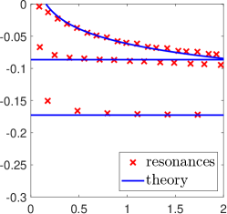
Figure 1: General setup of the potential function and resulting resonances. Upward arrows represent delta functions against the horizontal line $x\in\mathbb{R}$. The MATLAB plot comes from Example 4 case $c$ and demonstrates the presence of the multiple strings of resonances.

This paper improves the results of [5] for the problem described above. They found that resonances lie in strings on multiple logarithmic curves of the form $\operatorname{Im}z\sim-\gamma h\log(1/h)$ and specified $2^{N-1}-1$ possibilities for $\gamma$ determined by the parameters $x_{j}$, $\beta_{j}$. Here, we use the same tool of Newton polygons but a more precise calculation to find exactly which $\gamma$ occur. We improve the upper bound to $N-1$ and show it is sharp (Corollary 3), as well as provide a new interpretation of these strings (Theorem 2). We also show the existence of a dominant pair of delta functions governing the resonances closest to the real axis and prove all strings except this first one are flat up to $o(h)$.

Resonances lying on multiple logarithmic strings of the form $\operatorname{Im}z\sim-\gamma h\log(1/h)$ have been observed in various examples but remain poorly understood. These include delta functions on the half line [4] and in $\mathbb{R}^{d}$ [9]; singular, compactly supported potentials on the real line [15]; two obstacles in $\mathbb{R}^{2}$, one with a corner [3]; and manifolds with conic singularities [11]. At best, the equation and quantity of all possible $\gamma$ can be determined explicitly, but other examples have just one possible $\gamma$ known and/or resonance-free regions. This paper provides a simple but well understood example to suggest approaches for more complicated problems. One such consistent pattern is the length of some longest geodesic in the denominator of $\gamma$, most explicitly in [11] as the longest trajectory between cone points. We observe a similar form but with a dependence on the strength of singularity like in [15].

Another motivation of our work is to a greater understanding of delta functions. Their application to quantum corrals and leaky quantum graphs have been studied extensively in [9]. In one dimension, multiple delta functions have been used to approximate general smooth potentials [12]. Other recent studies of $N>2$ delta functions in one dimension include [14, 7, 8], but we are not aware of any in the semiclassical regime besides [5] and [4].

2 Results

We summarize and interpret the results below. Then, we briefly define Newton polygons before presenting the main theorems. Examples, open questions, and an outline of the proof subsequently follow.

• Resonances lie in strings of the form $\operatorname{Im}z\sim-\gamma h\log(1/h)$ with $\gamma$ determined in an indirect but explicit way from the parameters (Theorem 1). We prove these resonances exist (Theorem 4) and provide numerical evidence that such resonances are the only ones that exist.

• The strings of resonances correspond to a complete and disjoint partitioning of a line segment with Dirac deltas at interval endpoints. More precisely, each $\gamma$ incorporates parameters from precisely two Dirac deltas, and the intervals between these pairs of deltas form the partition (Theorem 2).

• The string closest to the real axis, hence containing the longest living resonances, is the only string with logarithmic shape (Corollary 5). Its corresponding pair of Dirac deltas minimize their combined strength divided by the distance between them, among all pairs.

2.1 Newton polygon and theorems

Definition 1.

The Newton polygon of a set of points $\{(\lambda_{i},\nu_{i})\}_{i}$ is the convex hull of the epigraph of the points. In other words, it is the shape of a rubber band around these points and stretched to $(0,\infty)$.

Newton polygons are a tool from commutative algebra for investigating valuations of polynomial roots. However, we use them to encapsulate several minimization conditions and inequalities. As typical, the important feature is the non-infinite slopes.

Definition 2.

Our Newton polygon is the one constructed from the following set of points:

$$\{\big{(}2(x_{k}-x_{j}),\>\beta_{j}+\beta_{k}\big{)}:1\leq j<k\leq N\}\cup\{(0,0)\}$$ (2.1)

Let $\Gamma$ be the set of its non-infinite slopes.

Figure 2: Example of our chosen Newton polygon from the parameters on left, labeled on each delta function (represented by arrows). Note that larger $\beta_{j}$ implies weaker delta functions, since $h\rightarrow 0$ in $C_{j}h^{\beta_{j}+1}$. We continue displaying Example 4 part $c$ as a case with several strings of resonances.

Theorem 1.

Resonances on log curves $h\log(1/h)$ must correspond to slopes of our Newton polygon. More precisely, if $z=z(h)=z(h_{j})$ is a sequence of resonances with $\operatorname{Re}z\in U\Subset(0,\infty)$ and $\operatorname{Im}z=-\gamma h\log(1/h)+O(h)$ as $h_{j}\rightarrow 0$, then $\gamma\in\Gamma$.

We define a string of resonances as the sequence $z(h_{j})$ corresponding to a value $\gamma$, which in turn comes from the Newton polygon. This result was known in [5], but we can now describe the slopes of the Newton polygon much more precisely. First, it is convenient and sometimes necessary to impose the following constraint, which we take as given throughout.

Assumption 1.

Let the parameters $\beta_{j},x_{j}$ be given such that the non-infinite slopes of the Newton polygon are unique. In other words, for any three collinear points in (eq 2.1), at least one is in the interior of the polygon.

Example 8 shows that without this assumption, strings of higher multiplicities emerge. Fortunately, this case is rare, in the sense that the parameters following this assumption are generic in the parameter space, since we need only avoid a finite set of linear equations. Our next notation gives the structure of these slopes.

$$\gamma_{jk} :=\frac{\beta_{k}+\beta_{j}}{2|x_{k}-x_{j}|} \widetilde{\gamma}_{jk} :=\frac{|\beta_{k}-\beta_{j}|}{2|x_{k}-x_{j}|}$$ (2.2)

For the moment, the simplest slope to identify on the Newton polygon is the leftmost one, starting from $(0,0)$. This point must be the bottom left corner of the Newton polygon because $\beta_{j}>0$, the slope from it to a point in (eq 2.1) must be of the form $\gamma_{jk}$, and the convex hull contains the minimum $\gamma_{jk}$.

Definition 3.

The dominant pair of delta potentials, indexed $J,K$, is the one which minimizes the value $\gamma_{jk}$ among all pairs $j,k$. Assumption 1 guarantees $J,K$ are uniquely determined by this condition:

$$\forall j,k\quad\gamma_{JK}\leq\gamma_{jk}\quad\text{with equality iff}\quad J=j,K=k$$ (2.3)

Since slopes on our Newton Polygon are increasing, $\gamma_{JK}$ is the minimum value of $\Gamma$. It corresponds to the string closest to the real axis and hence the longest living resonances. The interpretation of the remaining strings of resonances is given by the following theorem.

Theorem 2.

There exists an integer partitioning of $[1,N]$ i.e. $1=j_{1}<...<j_{n}=N$ such that the slopes of our Newton polygon are elements of the following set.

$$\Gamma=\big{\{}\gamma_{JK}\big{\}}\cup\Big{\{}\widetilde{\gamma}_{j_{i}j_{i+1}}:i=1,...,n-1,\>\>\>i\neq I\Big{\}}$$ (2.4)

These indices include the dominant pair at some $I$ with $j_{I}=J$, $j_{I+1}=K$.

Corollary 3.

There are at most $N-1$ strings of resonances. Furthermore, the $K-J-1$ delta functions between the dominant pair cannot contribute strings.

$$\text{\# strings of resonances}\leq N-K+J$$ (2.5)

This inequality is sharp by Example 2. Equality holds for $N=2$, $N=3$, and (Example 4) most cases of $N=4$.

Essentially, there is a string of resonances following $-\gamma h\log(1/h)$ if and only if $\gamma$ is a slope on the Newton polygon. Theorem 1 gives the forward implication, while Theorem 4 gives the converse. The distinction between resonances on the dominant string $z_{m}$ and on the remaining strings $\widetilde{z}_{m}$ becomes clearer in the equations of Corollary 5.

Theorem 4.

There exists a string of resonances corresponding to every $\gamma\in\Gamma$. More precisely, we have that for any $M$ large, there exists $h_{0}$ small such that for all $h\in(0,h_{0})$, any integer $m$ satisfying $\pi hm/(x_{k}-x_{j})\in[\frac{2}{M},\frac{M}{2}]$ gives a resonance in one of the following forms.

$$z_{m} =\frac{\pi hm}{x_{k}-x_{j}}-i\gamma_{jk}h\log(1/h)+\frac{ih}{2(x_{k}-x_{j})}\log\left(\frac{-C_{j}C_{k}(x_{k}-x_{j})^{2}}{4\pi^{2}h^{2}m^{2}}\right)+o(h)$$ (2.6)

$$\widetilde{z}_{m} =\frac{\pi hm}{x_{k}-x_{j}}-i\widetilde{\gamma}_{jk}h\log(1/h)+\frac{ih}{2(x_{k}-x_{j})}\log\left(\frac{-C_{j}}{C_{k}}\right)+o(h)$$ (2.7)

The dominant string is given by (eq 2.6) and the remaining strings by (eq 2.7).

Corollary 5.

Resonances on the dominant string are logarithmic with respect to $\operatorname{Im}z$ against $\operatorname{Re}z$, while the remaining strings are flat up to $o(h)$.

$$\operatorname{Im}z_{m} =-\frac{h}{x_{K}-x_{J}}\log\left(\frac{2\operatorname{Re}z}{\sqrt{|C_{J}C_{K}|}}\right)-\gamma_{JK}h\log(1/h)+o(h)$$ (2.8)

$$\operatorname{Im}\widetilde{z}_{m} =-\frac{h}{x_{k}-x_{j}}\log\left(\sqrt{\left|\frac{C_{j}}{C_{k}}\right|}\right)-\widetilde{\gamma}_{jk}h\log(1/h)+o(h)$$ (2.9)

We can now revisit the MATLAB plot in Figure 1 as referring to the theory given by Corollary 5. The three strings of resonances here correspond to the three slopes in the Newton polygon of Figure 2. We provide many more generic and concrete examples below.

2.2 Examples and discussion

Our first example sets all $\beta_{j}$ equal to investigate the role of position $x_{j}$. We find there is always one string of resonances, resolving a conjecture of [5]. Since the largest distance is preferred, there is resemblance with the longest geodesic behavior of [11]. Also note that the parameters $C_{j}$ are insignificant here and are only considered in Example 10, implying the choice of $h$-dependent barriers is crucial to the result.

Example 1.

Consider equal strength parameters $\beta_{1}=...=\beta_{N}$. Per Theorem 2, the dominant pair is $J=1$, $K=N$, since $\beta_{j}+\beta_{k}$ is constant and $\frac{1}{x_{k}-x_{j}}$ favors the largest distance. This alone implies there is exactly one string of resonances, since $N-K+J=1$ in Corollary 3. See Example 4 part $a$ for a more concrete example.

Example 2.

To achieve the maximum $N-1$ strings in Corollary 3, we consider highly unequal strength deltas. If $\beta_{j}<<\beta_{j+1}$ and $x_{j+1}-x_{j}=1$ for all $j$, e.g. $\beta_{j}=10^{-j}$, then points in (eq 2.1) are $(\beta_{j}+\beta_{k})/2(x_{k}-x_{j})\approx\beta_{k}/2(k-j)$. We show $K-J=1$ in the figure, and it follows that (eq 2.5) is sharp for any $J,K$ by placing much weaker strings between the dominant pair $J=1$, $K=2$.

The case of $N=2$ always produces one string of resonances, so we turn to $N=3$ to demonstrate the emergence of multiple strings of resonances with the Newton polygon.

Example 3.

Consider three delta functions at $x_{1}=0$, $x_{2}=4$, $x_{3}=6$ with asymptotic strength $\beta_{1}=0.5$, $\beta_{2}=0.5$, $\beta_{3}=2.0$. We simplify the other constants by setting $C_{1}=C_{2}=C_{3}=1$, and we only need a relatively large $h=0.1$ to see agreement with theory. We discuss each of the following three figures in turn.

1. We first draw these parameters. The explicit potential is $V(x)=\sum_{j=1}^{N}C_{j}h^{\beta_{j}+1}\delta(x-x_{j})\approx 0.03\delta(x)+0.03\delta(x-4)+0.001\delta(x-6)$. Among $\gamma_{12}=0.125$, $\gamma_{13}\approx 0.208$, and $\gamma_{23}=0.625$, we see that $\gamma_{12}$ is minimal so $J=1$, $K=2$ is dominant.

2. The Newton polygon is constructed of points $\big{(}2(x_{k}-x_{j}),\>\beta_{j}+\beta_{k}\big{)}$ for all pairs $j<k$. Namely, these $(j,k)$ are $(1,2)$, $(2,3)$, and $(1,3)$, labeled as black dots on the polygon. We also see that the slopes are $\gamma_{12}$ and $\widetilde{\gamma}_{23}$.

3. As predicted, there are two distinct strings of resonances in the numerical computation by MATLAB. We elaborate on why the bottom string here has fewer resonances than the dominant string in Example 7. The theory lines colored blue correspond to the two blue slopes of the Newton polygon and to the two blue brackets of the potential function sketch.

The cases of $N=2$ and $N=3$ were well understood in [5] and [14] among others, but a wider range of conditions emerges at $N=4$. In fact, it inspired several of our results. It is the first case where the choice of dominant pair does not uniquely give the number of strings of resonances, specifically in case $d$ and $e$ below, yet the dominant pair characterizes cases $a-c$, Hence, it shows how strongly the dominant pair affects the resonances.

Example 4.

Consider $N=4$. There are five cases of how strings correspond to intervals, up to symmetry, and the dominant pair distinguishes three of them. Brackets correspond to slopes on the Newton polygon, and the largest bracket signifies the dominant pair. We take $h=0.1$ and $C_{1}=C_{2}=C_{3}=C_{4}=1$. Note again that larger $\beta_{j}$ implies weaker delta functions, in how we draw the arrows.

1. Dominant $J=1$, $K=4$: This is a particular case of Example 1. The middle two delta functions are overshadowed.

   

2. Dominant $J=1$, $K=3$. The strongest delta function by $\beta_{3}$ pairs with the farthest away of the remaining deltas at $x_{1}$ to form the dominant pair.

   

3. Dominant $J=2$, $K=3$: The middle position of the dominant delta functions forces three strings to occur.

   

4. Dominant $J=1$, $K=2$ with 2 strings: This is the only case for $N=4$ with strict inequality in (eq 2.5), since there are 2 strings but $2<4-2+1=3$. It is also the only case where the dominant pair does not uniquely determine the number of strings, by comparison with the subsequent part e.

   

5. Dominant $J=1$, $K=2$ with 3 strings: Only a slight change in the point $(4,2.5)$ in the previous case to $(5,2.5)$ is needed to change the number of strings. Nevertheless, the slopes of the polygon are hard to distinguish, and the strings are correspondingly close.

   

We continue our discussion with open problems. A technical limitation of the current results is that we only consider resonances of the form $\operatorname{Im}z=-\gamma h\log(1/h)+O(h)$, but numerical evidence suggest these are the only ones that exist.

Conjecture 1.

Theorem 1 applies to all resonances such that $\operatorname{Re}z\in U\Subset(0,\infty)$ and $\operatorname{Im}z<0$.

Another observed but omitted behavior is the regime $\operatorname{Re}z\rightarrow\infty$. This would help explain the deviation from theory when predicted strings intersect and seemingly merge, elaborated in Example 9. This limit seems to compete with the limit $h\rightarrow 0$.

Conjecture 2.

As $\operatorname{Re}z\rightarrow\infty$, all strings coalesce into a single log curve corresponding to the outermost delta functions.

$$\operatorname{Im}z=-\frac{h}{x_{N}-x_{1}}\log\operatorname{Re}z+O(1)$$ (2.10)

We also have several broader ideas concerning the interpretation.

1. How do strings of resonances correspond to intervals? We found that the parameters determining the equation of a string correspond to intervals, but it is unclear if this correspondence holds for the wave function. It would be interesting if the resonant state of resonances on different strings would be concentrated in those respective intervals.

2. What about bound states? If bound states exist by $C_{j}<0$, [8] showed there are at most $N$ bound states by using that an $N\times N$ matrix has at most $N$ eigenvalues. If bound states had some association with strings of resonances, the formula here could help determine the exact number of bound states analytically from the parameters.

3. Do the results generalize to delta functions on graphs? Strong delta functions can obscure weaker ones from contributing strings, but this generalization would determine whether the effect is from collinearity or more organic to the wave function. Two ideas to test the role of distance and strength are in Figure 3.

Figure 3: Two examples of delta functions on graphs of interest to an open problem. The left case considers equal strength deltas connected by unequal length line segments, while the right case considers equal length line segments connecting unequal strength deltas.

2.3 Outline

Section 1 sketched the mathematical setup and provided background, and section 2 precisely stated the main results. The remainder of the paper contains the proofs, besides the code included in section 9.

1. The continuity and jump conditions which characterize Dirac deltas give an algebraic equation for the resonances in the form of a large determinant. This setup is a routine calculation.

2. We explicitly compute this determinant in Lemma 4.1 by simplifying into a tridiagonal form reminiscent of a Jacobi matrix, then applying induction. The primary difficulty is choosing notation suitable to manage it.

3. We use the assumptions in Theorem 1 to asymptotically simplify the determinant in Lemma 5.1. The Newton polygon arises naturally from an equation of asymptotically differing terms having at least two largest terms to balance out.

4. Theorem 2 on the Newton polygon depends only on its construction and the geometric setup of the delta functions, not the wave function. Nevertheless, it is ultimately this geometric argument that gives the interpretation of the strings of resonances, such as Corollary 3.

5. Existence of resonances in Theorem 4 is given by Rouché’s theorem. A mixed rational and exponential equation is simplified by precisely finding the largest terms from Lemma 5.2 and Theorem 2.

6. We complete the proof of Theorem 4 by refining the asymptotics.

7. Lastly, we discuss the numerical fit with theory and provide the code to numerically compute these resonances.

3 Delta functions: the algebraic equation for the resonances

This section sketches the routine derivation of the equation determining $z$. See chapter 2 of [10] for an introduction to delta functions as potentials and chapter 2 of [6] for background on resonances. The ansatz below solves the Schrödinger equation (eq 1.1) in the sense of distributions:

$$u(x)=v_{j}^{+}e^{izx/h}+v_{j}^{-}e^{-izx/h}\text{ in }(x_{j},x_{j+1})$$ (3.1)

The unknown coefficients $v_{j}^{\pm}$ are associated right right-travelling $v^{+}$ and left-travelling $v^{-}$ components in the time-dependent equation, depicted in Figure 4. For convenience, define the endpoints in (eq 3.1) as $x_{0}=-\infty$ and $x_{N+1}=\infty$.

Figure 4: General setup of Figure 1 annotated with coefficients from the ansatz (eq 3.1). Between delta functions as up arrows, coefficients $v_{j}^{+}$ correspond to right travelling waves and $v_{j}^{-}$ left travelling.

Resonances are restricted to outgoing solutions, defined as having no incoming component from the unbounded edges, implying $v_{0}^{+}=v_{N}^{-}=0$ but not all $v_{j}^{\pm}$ are zero. The remaining coefficients are determined by continuity and jump conditions created by the delta functions:

$$\begin{cases}u(x_{j}^{-})-u(x_{j}^{+})=0\\ h^{2}\big{(}u^{\prime}(x_{j}^{-})-u^{\prime}(x_{j}^{+})\big{)}+C_{j}h^{1+\beta_{j}}u(x_{j})=0\end{cases}$$ (3.2)

We use the ansatz (eq 3.1) to write this more explicitly and group terms by the unknown coefficients $v_{j}^{\pm}$.

$$\begin{cases}v_{j-1}^{-}e^{-ix_{j}z/h}+v_{j-1}^{+}e^{ix_{j}z/h}-v_{j}^{-}e^{-ix_{j}z/h}-v_{j}^{+}e^{ix_{j}z/h}=0\\ -izv_{j-1}^{-}e^{-ix_{j}z/h}izv_{j-1}^{+}e^{ix_{j}z/h}+(-iz+(iz+C_{j}h^{\beta_{j}})v_{j}^{-}e^{-ix_{j}z/h}+C_{j}h^{\beta_{j}})v_{j}^{+}e^{ix_{j}z/h}=0\end{cases}$$

We abbreviate the exponential term with the notation

$$\omega:=e^{iz/h}$$ (3.3)

cautioning that $\omega=w^{-1}$ compared to the notation of [5]. We further simplify it by multiplying through $e^{-ix_{j}z/h}$:

$$\begin{cases}v_{j-1}^{-}\omega^{-2x_{j}}+v_{j-1}^{+}-v_{j}^{-}\omega^{-2x_{j}}-v_{j}^{+}=0\\ -izv_{j-1}^{-}\omega^{-2x_{j}}+izv_{j-1}^{+}+(iz+C_{j}h^{\beta_{j}})v_{j}^{-}\omega^{-2x_{j}}+(-iz+C_{j}h^{\beta_{j}})v_{j}^{+}=0\end{cases}$$

We write this system in matrix notation to emphasize its linearity with respect to $v_{j}^{\pm}$. Also, recall that coefficients $v_{0}^{+},v_{N}^{-}$ are omitted, and the order of the remaining $v_{0}^{-},v_{1}^{-},v_{1}^{+},...$ is chosen for later convenience. $\begin{pmatrix}\omega^{-2x_{1}}&-\omega^{-2x_{1}}&-1&0&0&\ldots&0\\ -iz\omega^{-2x_{1}}&(iz+C_{1}h^{\beta_{1}})\omega^{-2x_{1}}&(-iz+C_{1}h^{\beta_{1}})&0&0&\ldots&0\\ \vspace{-7pt}0&\omega^{-2x_{2}}&1&-\omega^{-2x_{2}}&-1&&0\\ \vspace{-7pt}0&-iz\omega^{-2x_{2}}&iz&(iz+C_{2}h^{\beta_{2}})\omega^{-2x_{2}}&(-iz+C_{2}h^{\beta_{2}})&\ddots&0\\ \vdots&\vdots&\vdots&\vdots&\vdots&\ddots&-1\\ 0&0&0&0&0&&(-iz+C_{N}h^{\beta_{N}})\end{pmatrix}\begin{pmatrix}v_{0}^{-}\\ v_{1}^{-}\\ v_{1}^{+}\\ v_{2}^{-}\\ v_{2}^{+}\\ \vdots\\ v_{N}^{+}\end{pmatrix}=0$
We have $2N$ equations, two for each delta function, and $2N$ unknowns $v_{j}^{\pm}$, two for each $N+1$ interval between delta functions but excluding $v_{0}^{+}=v_{N}^{-}=0$. To find a nontrivial solution to the last unknown $z$, we require the null space against the $v_{j}^{\pm}$ vector is trivial, or equivalently that the determinant of the coefficients of $v_{j}^{\pm}$ in matrix form is 0.

$$D_{N}:=$$ (3.4)

$$\det\begin{pmatrix}\omega^{-2x_{1}}&-\omega^{-2x_{1}}&-1&0&0&\ldots&0\\ -iz\omega^{-2x_{1}}&(iz+C_{1}h^{\beta_{1}})\omega^{-2x_{1}}&(-iz+C_{1}h^{\beta_{1}})&0&0&\ldots&0\\ \vspace{-7pt}0&\omega^{-2x_{2}}&1&-\omega^{-2x_{2}}&-1&&0\\ \vspace{-7pt}0&-iz\omega^{-2x_{2}}&iz&(iz+C_{2}h^{\beta_{2}})\omega^{-2x_{2}}&(-iz+C_{2}h^{\beta_{2}})&\ddots&0\\ \vdots&\vdots&\vdots&\vdots&\vdots&\ddots&-1\\ 0&0&0&0&0&&(-iz+C_{N}h^{\beta_{N}})\end{pmatrix}$$

The remainder of the paper is essentially an analysis of this equation.

4 Determinant formula: simplifying the equation for resonances

A mundane but critical step in investigating $z$ is simplifying the determinant formula in (eq 3.4). This is primarily an exercise in notation, starting with the following:

$$R_{j} :=\frac{C_{j}h^{\beta}_{j}}{2iz-C_{j}h^{\beta}_{j}} T_{j} :=\frac{2iz}{2iz-C_{j}h^{\beta}_{j}}$$ (4.1)

The variables $R_{j}$ and $T_{j}$ are suggestively named for reflection and transmission, and their interpretation is provided later in (eq 4.8). We first present the main result of this section, along with the notation convenient to succinctly prove it.

Lemma 4.1.

The determinant given by (eq 3.4) is the following, aided by the notation above and the index set below.

$$\frac{1}{c}D_{N} =1+\sum_{n=1}^{\lfloor N/2\rfloor}(-1)^{n}\sum_{\mathscr{I}_{n}^{N}}R_{j_{1}}^{k_{1}}\cdot...\cdot R_{j_{n}}^{k_{n}}$$ (4.2)

$$R_{j}^{k} :=\begin{cases}R_{j}R_{k}\omega^{2(x_{k}-x_{j})}&k=j+1\\ R_{j}(T_{j+1}+R_{j+1})\cdot...\cdot(T_{k-1}+R_{k-1})\cdot R_{k}\omega^{2(x_{k}-x_{j})}&k>j+1\end{cases}$$ (4.3)

$$\mathscr{I}_{n}^{N} :=\Big{\{}\{j_{1},k_{1},...,j_{n},k_{n}\}:j_{i},k_{i}\in\mathbb{N}\text{ and }\forall i=1,...,(n-1)\>\>\>1\leq j_{i}<k_{i}<j_{i+1}<k_{i+1}\leq N\Big{\}}$$ (4.4)

$$c :=-\prod_{j=1}^{N}\frac{\omega^{-2x_{j}}}{2iz-C_{1}h^{\beta_{1}}}$$ (4.5)

Example 5.

We demonstrate (eq 4.2) for $N=2$ below. With $n=1$ and $\mathscr{I}_{1}^{2}=\big{\{}\{1,2\}\}$, there are just two terms.

$$\frac{1}{c}D_{2}=1-R_{1}^{2}=1-R_{1}R_{2}\omega^{2(x_{2}-x_{1})} =0$$

$$\frac{C_{1}h^{\beta_{1}}}{2iz-C_{1}h^{\beta_{1}}}\frac{C_{2}h^{\beta_{2}}}{2iz-C_{2}h^{\beta_{2}}}e^{2i(x_{2}-x_{1})z/h} =1$$

Example 6.

We compute $D_{4}$ to demonstrate the terms from $n=2$. Fortunately, there is only one element in the new index set $\mathscr{I}_{2}^{4}=\big{\{}\{1,2,3,4\}\big{\}}$.

$$\frac{1}{c}D_{4} =1-\sum_{\mathscr{I}_{1}^{4}}R_{j_{1}}^{k_{1}}+\sum_{\mathscr{I}_{2}^{4}}R_{j_{1}}^{k_{1}}\cdot R_{j_{2}}^{k_{2}}$$

$$=1-\Big{(}R_{1}R_{2}\omega^{2(x_{2}-x_{1})}+R_{2}R_{3}\omega^{2(x_{3}-x_{2})}+R_{3}R_{4}\omega^{2(x_{4}-x_{3})}+R_{1}(R_{2}+T_{3})R_{3}\omega^{2(x_{3}-x_{1})}+$$

$$\quad+R_{2}(R_{3}+T_{3})R_{4}\omega^{2(x_{4}-x_{2})}+R_{1}(R_{2}+T_{2})(R_{3}+T_{3})R_{4}\omega^{2(x_{4}-x_{1})}\Big{)}+R_{1}R_{2}R_{3}R_{4}\omega^{2(x_{2}-x_{1}+x_{4}-x_{3})}$$

We proceed with the proof of Lemma 4.1. It is sufficient for our later use that some products of $R_{j}^{k}$ are the terms that appear in $D_{N}$, but we describe the full formula for concreteness. There are two distinct steps: row reduction to tridiagonal form and induction from its recursive relationship.

Proof.

We first simplify (eq 3.4) with row reduction to a tridiagonal form. The steps are adding the odd rows $\cdot iz$ into the even rows, then adding the even rows $\cdot\frac{1}{-2iz+C_{1}h^{\beta_{1}}}$ into the odd rows.

$$\det\begin{pmatrix}\omega^{-2x_{1}}&-\omega^{-2x_{1}}&-1&0&0&\ldots&0\\ -iz\omega^{-2x_{1}}&(iz+C_{1}h^{\beta_{1}})\omega^{-2x_{1}}&(-iz+C_{1}h^{\beta_{1}})&0&0&\ldots&0\\ \vspace{-7pt}0&\omega^{-2x_{2}}&1&-\omega^{-2x_{2}}&-1&&0\\ \vspace{-7pt}0&-iz\omega^{-2x_{2}}&iz&(iz+C_{2}h^{\beta_{2}})\omega^{-2x_{2}}&(-iz+C_{2}h^{\beta_{2}})&\ddots&0\\ \vdots&\vdots&\vdots&\vdots&\vdots&\ddots&-1\\ 0&0&0&0&0&&(-iz+C_{N}h^{\beta_{N}})\end{pmatrix}$$

$$= \det\begin{pmatrix}\omega^{-2x_{1}}&-\omega^{-2x_{1}}&-1&0&0&\ldots&0\\ 0&C_{1}h^{\beta_{1}}\omega^{-2x_{1}}&(-2iz+C_{1}h^{\beta_{1}})&0&0&\ldots&0\\ \vspace{-7pt}0&\omega^{-2x_{2}}&1&-\omega^{-2x_{2}}&-1&&0\\ \vspace{-7pt}0&0&2iz&C_{2}h^{\beta_{2}}\omega^{-2x_{2}}&(-2iz+C_{2}h^{\beta_{2}})&\ddots&0\\ \vdots&\vdots&\vdots&\vdots&\vdots&\ddots&-1\\ 0&0&0&0&0&&(-2iz+C_{N}h^{\beta_{N}})\end{pmatrix}$$

$$= \det\begin{pmatrix}\omega^{-2x_{1}}&\frac{2iz}{-2iz+C_{1}h^{\beta_{1}}}\omega^{-2x_{1}}&0&0&0&\ldots&0\\ 0&C_{1}h^{\beta_{1}}\omega^{-2x_{1}}&(-2iz+C_{1}h^{\beta_{1}})&0&0&\ldots&0\\ \vspace{-7pt}0&\omega^{-2x_{2}}&\frac{C_{2}h^{\beta_{2}}}{-2iz+C_{2}h^{\beta_{2}}}&\frac{2iz}{-2iz+C_{2}h^{\beta_{2}}}\omega^{-2x_{2}}&0&&0\\ \vspace{-7pt}0&0&2iz&C_{2}h^{\beta_{2}}\omega^{-2x_{2}}&(-2iz+C_{2}h^{\beta_{2}})&\ddots&0\\ \vdots&\vdots&\vdots&\vdots&\vdots&\ddots&0\\ 0&0&0&0&0&&(-2iz+C_{N}h^{\beta_{N}})\end{pmatrix}$$

Switching to the notation (eq 4.1) by outside scaling greatly simplifies the entries. This includes multiplying every row by $-1$, which cancels due to the even number of rows.

$$D_{N}= \prod_{j=1}^{N}\frac{1}{2iz-C_{j}h^{\beta_{j}}}\cdot\det\begin{pmatrix}\omega^{-2x_{1}}&-T_{1}\omega^{-2x_{1}}&0&0&0&\ldots&0\\ 0&R_{1}\omega^{-2x_{1}}&-1&0&0&\ldots&0\\ \vspace{-7pt}0&\omega^{-2x_{2}}&-R_{2}&-T_{2}\omega^{-2x_{2}}&0&&0\\ \vspace{-7pt}0&0&T_{2}&R_{2}\omega^{-2x_{2}}&-1&\ddots&0\\ \vdots&\vdots&\vdots&\vdots&\vdots&\ddots&0\\ 0&0&0&0&0&&-1\end{pmatrix}$$

$$= -\prod_{j=1}^{N}\frac{\omega^{-2x_{j}}}{2iz-C_{j}h^{\beta_{j}}}\cdot\det\begin{pmatrix}R_{1}\omega^{-2x_{1}}&-1&0&0&\ldots\\ \vspace{-7pt}1&-R_{2}\omega^{2x_{2}}&-T_{2}&0&\\ 0&T_{2}&R_{2}\omega^{-2x_{2}}&-1&\ddots\\ \vdots&\vdots&\vdots&\vdots&\ddots\end{pmatrix}$$

$$= c\det\begin{pmatrix}R_{1}\omega^{-2x_{1}}&-1&0&0&\ldots\\ \vspace{-7pt}1&-R_{2}\omega^{2x_{2}}&-T_{2}&0&\\ 0&T_{2}&R_{2}\omega^{-2x_{2}}&-1&\ddots\\ \vdots&\vdots&\vdots&\vdots&\ddots\end{pmatrix}$$

Lastly, present $D_{N}$ in an expanded form and introduce new notation for the subsequent computation.

$$\widetilde{D}_{N}:=\frac{1}{c}D_{N}=\det\begin{pmatrix}R_{1}\omega^{-2x_{1}}&-1&0&0&0&\ldots&0\\ 1&-R_{2}\omega^{2x_{2}}&-T_{2}&0&0&\ldots&0\\ 0&T_{2}&R_{2}\omega^{-2x_{2}}&-1&0&\ldots&0\\ 0&0&1&-R_{3}\omega^{2x_{3}}&-T_{3}&\ldots&0\\ \vdots&\vdots&\vdots&\ddots&\ddots&\ddots&\vdots\\ 0&0&0&\ldots&T_{N-1}&R_{N-1}\omega^{2x_{N-1}}&-1\\ 0&0&0&\ldots&0&1&-R_{N}\omega^{2x_{N}}\end{pmatrix}$$ (4.6)

Further row reduction could turn this tridiagonal matrix symmetric, hence into a Jacobi matrix. We were unable to find an explicit formula suited to the goal of (eq 4.2) in the literature, but the repeating entries in the main diagonal helps simplify it here. We set up a depth two recursion in the determinant (eq 4.6) and the same but one row/column smaller. The prior section simplified $\widetilde{D}_{N}$ to coming from a $2N-2$ square matrix, while $d_{N-1}$ is a $2(N-1)-1$ square matrix.

$$d_{N-1} :=\det\begin{pmatrix}R_{1}\omega^{-2x_{1}}&-1&&&\\ 1&\ddots&\ddots&&\\ &\ddots&R_{N-2}\omega^{-2x_{N-2}}&-1&\\ &&1&-R_{N-1}\omega^{2x_{N-1}}&-T_{N-1}\\ &&&T_{N-1}&R_{N-1}\omega^{-2x_{N-1}}\end{pmatrix}$$ (4.7)

In particular, cofactor expansion on the last column gives the following:

$$\widetilde{D}_{N}=-R_{N}\omega^{2x_{N}}d_{N-1}+\widetilde{D}_{N-1}$$

The key step is the reduction of coefficients in $d_{N-1}$, following from that reciprocals of $\omega^{-2x_{N-1}}$ cancel and $T_{j}^{2}-R_{j}^{2}=(T_{j}-R_{j})(T_{j}+R_{j})=R_{j}+T_{j}$ simplifies.

$$d_{N-1} =R_{N-1}\omega^{-2x_{N-1}}\widetilde{D}_{N-1}+T_{N-1}^{2}d_{N-2}$$

$$=R_{N-1}\omega^{-2x_{N-1}}(-R_{N-1}\omega^{2x_{N-1}}d_{N-2}+\widetilde{D}_{N-2})+T_{N-1}^{2}d_{N-2}$$

$$=(R_{N-1}+T_{N-1})d_{N-2}+R_{N-1}\omega^{-2x_{N-1}}\widetilde{D}_{N-2}$$

Iteratively plugging this into the recurrence for $\widetilde{D}_{N}$ eliminates all $d$ terms at the expense of creating a full order recurrence in $\widetilde{D}_{N}$.

$$\widetilde{D}_{N} =-R_{N}\omega^{2x_{N}}\big{(}(R_{N-1}+T_{N-1})d_{N-2}+R_{N-1}\omega^{-2x_{N-1}}\widetilde{D}_{N-2}\big{)}+\widetilde{D}_{N-1}$$

$$=\widetilde{D}_{N-1}-R_{N}R_{N-1}\omega^{2(x_{N}-x_{N-1})}\widetilde{D}_{N-2}-R_{N}(R_{N-1}+T_{N-1})\omega^{2x_{N}}d_{N-2}$$

$$=\widetilde{D}_{N-1}-R_{N}R_{N-1}\omega^{2(x_{N}-x_{N-1})}\widetilde{D}_{N-2}-R_{N}(R_{N-1}+T_{N-1})R_{N-2}\omega^{2(x_{N}-x_{N-2})}\widetilde{D}_{N-3}$$

$$\quad-R_{N}(R_{N-1}+T_{N-1})(R_{N-2}+T_{N-2})\omega^{2x_{N}}d_{N-3}$$

Then, we continue inductively until the base case $d_{1}=R_{1}\omega^{-2x_{1}}$.

$$\widetilde{D}_{N} =\widetilde{D}_{N-1}-R_{N-1}^{N}\widetilde{D}_{N-2}-R_{N-2}^{N}\widetilde{D}_{N-3}-...-R_{1}^{N}\widetilde{D}_{0}$$

$$=\widetilde{D}_{N-1}-\sum_{m=1}^{N-1}R_{N-m}^{N}\widetilde{D}_{N-m-1}$$

We see that the coefficient of $\widetilde{D}_{i}$ only has $R_{j}$ and $x_{j}$ terms with $j>i$. Also, the base case of $\widetilde{D}_{2}=1-R_{1}R_{2}\omega^{2(x_{2}-x_{1})}$ extrapolates to $\widetilde{D}_{1}=1$ and $\widetilde{D}_{0}=1$. We now perform induction to finish the proof. The base case is a simple $2\times 2$ determinant, and the meaning of formula (eq 4.2) demonstrated in Example 5.

$$\widetilde{D}_{2}=\det\begin{pmatrix}R_{1}\omega^{-2x_{1}}&-1\\ 1&-R_{2}\omega^{2x_{2}}\end{pmatrix}=-R_{1}R_{2}\omega^{2(x_{2}-x_{1})}+1$$

The step case follows from the recursion above. The key idea is that $\mathscr{I}_{n}^{N+1}$ can be decomposed into $\mathscr{I}_{n}^{N}$, which comes from $-\widetilde{D}_{N-1}$, and $\mathscr{I}_{n}^{N+1}\big{|}_{k_{n}=N+1}$, which comes from the remaining $m=1,...,N-1$ terms.

$$\widetilde{D}_{N+1} =\widetilde{D}_{N}-\sum_{m=1}^{N}R_{N-m+1}^{N+1}\widetilde{D}_{N-m}$$

$$=\widetilde{D}_{N}-\sum_{m=1}^{N}R_{N-m+1}^{N+1}\cdot\left(1+\sum_{n=1}^{\lfloor(N-m)/2\rfloor}\sum_{\mathscr{I}_{n}^{N-m}}(-1)^{n}R_{j_{1}}^{k_{1}}\cdot...\cdot R_{j_{n}}^{k_{n}}\right)$$

$$=\widetilde{D}_{N}-\sum_{m=1}^{N}\left(R_{N-m+1}^{N+1}+\sum_{n=1}^{\lfloor(N-m)/2\rfloor}\sum_{\mathscr{I}_{n}^{N-m}}(-1)^{n}R_{j_{1}}^{k_{1}}\cdot...\cdot R_{j_{n}}^{k_{n}}\cdot R_{N-m+1}^{N+1}\right)$$

$$=\widetilde{D}_{N}-\left(\sum_{\mathscr{I}_{1}^{N+1}}^{k_{1}=N+1}R_{j_{1}}^{N+1}+\sum_{n=2}^{\lfloor(N-1)/2\rfloor+1}\sum_{\mathscr{I}_{n}^{N+1}}^{k_{n}=N+1}(-1)^{n-1}R_{j_{1}}^{k_{1}}\cdot...\cdot R_{j_{n}}^{N+1}\right)$$

$$=\widetilde{D}_{N}-\left(\sum_{n=1}^{\lfloor(N+1)/2\rfloor}\sum_{\mathscr{I}_{n}^{N+1}}^{k_{n}=N+1}(-1)^{n-1}R_{j_{1}}^{k_{1}}\cdot...\cdot R_{j_{n}}^{N+1}\right)$$

$$=\left(1+\sum_{n=1}^{\lfloor N/2\rfloor}\sum_{\mathscr{I}_{n}^{N}}(-1)^{n}R_{j_{1}}^{k_{1}}\cdot...\cdot R_{j_{n}}^{k_{n}}\right)+\left(\sum_{n=1}^{\lfloor(N+1)/2\rfloor}\sum_{\mathscr{I}_{n}^{N+1}}^{k_{n}=N+1}(-1)^{n}R_{j_{1}}^{k_{1}}\cdot...\cdot R_{j_{n}}^{N+1}\right)$$

$$=1+\sum_{n=1}^{\lfloor(N+1)/2\rfloor}\sum_{\mathscr{I}_{n}^{N+1}}(-1)^{n}R_{j_{1}}^{k_{1}}\cdot...\cdot R_{j_{n}}^{k_{n}}$$

∎

In further discussion, we motivated the reductions by bringing the matrix into tridiagonal form and the (eq 4.1) notation as the most suitable abbreviations for this form. Alternatively, we could have isolated each $v_{j}^{\pm}$ and identified contributions from reflection at $x_{j}$ and transmission through $x_{j}$. However, $|R_{j}|^{2}$ and $|T_{j}|^{2}$ are not the reflection and transmission coefficients unless $N=1$. To derive (eq 4.8) from (eq 4.6), note that the vector $(v_{0}^{-},v_{1}^{-},v_{1}^{+},v_{2}^{-},v_{2}^{+},...,v_{N-1}^{+},v_{N}^{+})$ became $(v_{1}^{-},v_{1}^{+},v_{2}^{-},v_{2}^{+},...,v_{N-1}^{+})$ during the row reduction.

$$v_{j-1}^{-} =v_{j-1}^{+}R_{j}\omega^{2x_{j}}+T_{j}v_{j}^{-}$$ (4.8)

$$v_{j}^{+} =v_{j-1}^{+}T_{j}+R_{j}\omega^{-2x_{j}}v_{j}^{-}$$

Figure 5: Refinement of Figure 4 with transmission and reflection at the boundary. It depicts (eq 4.8), where arrow ends to $v_{j}^{+}$, $v_{j-1}^{-}$ are to the left-hand side and arrow starts from $v_{j-1}^{+}$, $v_{j}^{-}$ are on the right-hand side.

5 Proof of Theorem 1: motivating the Newton polygon

Since the determinant formula is a complicated transcendental equation, the limit $h\rightarrow 0$ is key to our new results. The conditions in Theorem 1 helps simplify $z$ terms in the exponents and denominator. The Newton polygon then emerges by comparing the largest terms.

Lemma 5.1.

Let $z(h_{j})$ be a sequence of resonances with $\operatorname{Re}z\in U\Subset(0,\infty)$ and $\operatorname{Im}z=-\gamma h\log(1/h)+O(h)$ as $h_{j}\rightarrow 0$. Then there exists $h_{0}$ such that for all $h\in(0,h_{0})$, (eq 4.2) simplifies to

$$\frac{1}{c}D_{N}=1+\sum_{1\leq j<k\leq N}\Big{(} \frac{C_{j}C_{k}}{4z^{2}}\cdot h^{\beta_{j}+\beta_{k}}+o(h^{\beta_{j}+\beta_{k}})\Big{)}\omega^{2(x_{k}-x_{j})}\text{,}$$ (5.1)

with the order of magnitude given by

$$\frac{C_{j}C_{k}}{4z^{2}}\cdot h^{\beta_{j}+\beta_{k}}\omega^{2(x_{k}-x_{j})}=O\big{(}h^{\beta_{j}+\beta_{k}-2(x_{k}-x_{j})\gamma}\big{)}\text{.}$$ (5.2)

Proof.

We used the $\omega,R_{j},T_{j}$ notation in Lemma 4.1 to simplify the determinant, and now we unwind them to see the $h$ dependence. We take $\lambda$ below to be a positive term of lengths, namely $2(x_{k}-x_{j})$ with $k>j$. The assumption on $\operatorname{Im}z$ is used to simplify $\omega$. A more weaker, more elegant assumption would be $\operatorname{Im}z\sim-\gamma h\log(1/h)$, but we require more control on the smaller terms due to the exponential.

$$\omega^{\lambda} =e^{iz\lambda/h}=e^{(-\operatorname{Im}z+i\operatorname{Re}z)\lambda/h}=e^{\gamma\lambda\log(1/h)+O(1)}e^{i(\operatorname{Re}z)\lambda/h}=h^{-\gamma\lambda}\cdot e^{i(\operatorname{Re}z)\lambda/h+O(1)}=O(h^{-\gamma\lambda})$$ (5.3)

We simplify $R_{j}$ and $T_{j}$ as a geometric series by taking $h_{0}$ small enough and by using the assumption on $\operatorname{Re}z$ not too close to 0 to bound $1/z$ from above. The binomial expansion of $R_{j}^{k}$ then reduces since $T_{j}$’s are larger than $R_{j}$’s.

$$R_{j} =\frac{C_{j}h^{\beta_{j}}}{2iz-C_{j}h^{\beta_{j}}}=\frac{C_{j}{h^{\beta}_{j}}}{2iz}\sum_{n=0}^{\infty}\left(\frac{C_{j}h^{\beta_{j}}}{2iz}\right)^{n}=\frac{C_{j}h^{\beta_{j}}}{2iz}+O(h^{2\beta_{j}})$$ (5.4)

$$T_{j} =\frac{2iz}{2iz-C_{j}h^{\beta_{j}}}=\sum_{n=0}^{\infty}\left(\frac{C_{j}h^{\beta_{j}}}{2iz}\right)^{n}=1+O(h^{\beta_{j}})$$ (5.5)

$$R_{j}(T_{j+1}+R_{j+1})\cdot...\cdot(T_{k-1}+R_{k-1})\cdot R_{k} =-\frac{C_{j}C_{k}}{4z^{2}}h^{\beta_{j}+\beta_{k}}+o(h^{\beta_{j}+\beta_{k}})$$ (5.6)

The factor $-C_{j}C_{k}/4z^{2}$ is $O(1)$ since $\operatorname{Re}z=O(1)$. This gives the order of magnitude of terms in (eq 5.2).

$$R_{j}^{k}=\Big{(}-\frac{C_{j}C_{k}}{4z^{2}}\cdot h^{\beta_{j}+\beta_{k}}+o(h^{\beta_{j}+\beta_{k}})\Big{)}\omega^{2(x_{k}-x_{j})}=O\Big{(}h^{\beta_{j}+\beta_{k}-2(x_{k}-x_{j})\gamma}\Big{)}$$

The last simplification is that the $n=1$ terms in (eq 4.2) are largest. In particular, any term in $\mathscr{I}_{n}^{N}$ with $n>1$ has an associated term in $\mathscr{I}_{1}^{N}$ which is asymptotically larger.

$$R_{j_{1}}^{k_{1}}\cdot...\cdot R_{j_{n}}^{k_{n}} =O\Big{(}h^{\beta_{j_{1}}+\beta_{k_{1}}+...+\beta_{j_{n}}+\beta_{k_{n}}-\gamma(x_{k_{1}}-x_{j_{1}}+...+x_{k_{n}}-x_{j_{n}})}\Big{)}$$

$$=o\Big{(}h^{\beta_{j_{1}}+\beta_{k_{n}}-\gamma(x_{k_{n}}-x_{j_{1}})}\Big{)}$$

$$R_{j_{1}}^{k_{n}} =O\Big{(}h^{\beta_{j_{1}}+\beta_{k_{n}}-\gamma(x_{k_{n}}-x_{j_{1}})}\Big{)}$$

The result (eq 5.1) follows after combining these results:

$$\frac{1}{c}D_{N} =1+\sum_{n=1}^{\lfloor N/2\rfloor}(-1)^{n}\sum_{\mathscr{I}_{n}^{N}}R_{j_{1}}^{k_{1}}\cdot...\cdot R_{j_{n}}^{k_{n}}$$

$$=1+\sum_{\mathscr{I}_{1}^{N}}(-R_{j_{1}}^{k_{1}})+\text{lower order terms}$$

$$=1+\sum_{1\leq j<k\leq N}\Big{(}\frac{C_{j}C_{k}}{4z^{2}}\cdot h^{\beta_{j}+\beta_{k}}+o(h^{\beta_{j}+\beta_{k}})\Big{)}\omega^{2(x_{k}-x_{j})}$$

Lastly, we can ignore the constant $c$ in $D_{N}=0$ since $\operatorname{Re}z$ away from 0 guarantees $\frac{1}{c}$ is bounded above.

∎

We now complete the proof of Theorem 1 and see how the Newton polygon emerges from Lemma 5.1.

Proof of Theorem 1.

Returning to the notation of Definition 1, let $\nu_{i}=\beta_{j}+\beta_{k}$, $\lambda_{i}=x_{k}-x_{j}$, and $c_{i}=O(1)$ for some indexing $i$. Then (eq 5.1) can be expressed as the following.

$$\frac{1}{c}D_{N}=\sum_{i}\Big{(}c_{i}h^{\nu_{i}-\gamma\lambda_{i}}+o(h^{\nu_{i}-\gamma\lambda_{i}})\Big{)}$$ (5.7)

The insight from [5] is that there must be at least two commensurate terms of greatest magnitude for $D_{N}=0$ to be satisfied. Asymptotically, this means two of the exponents of $h$ are equal and minimal.

$$\exists\>j,k\quad\nu_{j}-\gamma\lambda_{j}=\nu_{k}-\gamma\lambda_{k}=\min_{i}\nu_{i}-\gamma\lambda_{i}$$ (5.8)

After solving for $\gamma$, we see it is the slope between points $(\lambda_{j},\nu_{j})$ and $(\lambda_{k},\nu_{k})$ and express the minimality condition in a similar form. To simplify sign considerations, the cases $\lambda_{i}\geq\lambda_{j}$ and $\lambda_{i}\leq\lambda_{k}$ are equivalent by symmetry, so assume the former without loss of generality. Also assuming $\lambda_{j}<\lambda_{k}$, we have that $\lambda_{k}-\lambda_{j}$ and $\lambda_{i}-\lambda_{j}$ are both positive.

$$\gamma=\frac{\nu_{k}-\nu_{j}}{\lambda_{k}-\lambda_{j}}\leq\frac{\nu_{i}-\nu_{j}}{\lambda_{i}-\lambda_{j}}$$

We will visualize the possibilities of $\gamma$ with the Newton polygon. The minimality condition has the geometric interpretation that the segment $(\lambda_{j},\nu_{j})$ to $(\lambda_{k},\nu_{k})$ is on the Newton polygon of the points $(\lambda_{i},\nu_{i})$. This is because lines on the lower convex hull have smaller slope than lines into the interior, and the ordering $\lambda_{j}\leq\lambda_{i}$ ensures the slope is defined in the natural direction.

Figure 6: A Newton polygon, as defined in Definition 1 and more general than the specific Newton polygon in Definition 2. Note that the slope from points indexed $j$ to $k$ is smaller than the slope from $j$ to $i$ on the right and in the interior.

Lastly, we note that $\nu=\beta_{j}+\beta_{k}$ and $\lambda=2(x_{k}-x_{j})$ over $1\leq j<k\leq N$, with $(0,0)$ for the 1 term, is indeed our particular Newton polygon in Definition 2. Hence, under the conditions of Lemma 5.1, we have $\gamma\in\Gamma$. ∎

We have now connected resonances of logarithmic form to slopes of the Newton polygon, but the discussion above says more about the structure in Lemma 5.1. We return to it during the proof of Theorem 4 with the following link.

Lemma 5.2.

For any $\gamma^{*}\in\Gamma$, denote $\nu_{j}-\gamma^{*}\lambda_{j}$ and $\nu_{k}-\gamma^{*}\lambda_{k}$ as the equal and minimum exponents in (eq 5.8). There exists $\epsilon$ such that the exponents $\nu_{j}-\gamma\lambda_{j}$ and $\nu_{k}-\gamma\lambda_{k}$ remain minimal, though not necessarily equal, for all $\gamma$ near $\gamma^{*}$ as follows:

$$\gamma\in[\gamma^{*}-\epsilon,\gamma^{*}+\epsilon]$$ (5.9)

Let $z(h_{j})$ be a sequence of resonances with $\operatorname{Re}z\in U\Subset(0,\infty)$ and $\operatorname{Im}z=-\gamma h\log(1/h)+O(h)$ as $h_{j}\rightarrow 0$. Then the largest terms in (eq 5.1) are the two corresponding to $(\nu_{j},\lambda_{j})$ and $(\nu_{k},\lambda_{k})$.

Proof.

Figure 7 is central to the proof. It depicts the exponents $\beta_{j}+\beta_{k}-2\gamma(x_{k}-x_{j})$ as a function of $\gamma$ to clarify how we find the largest term for any $\gamma$, even though $\gamma\in\Gamma$ is a necessary condition for $z(h_{j})$ to be resonances.

Figure 7: A Newton polygon compared to the exponents of $h$ graphed against $\gamma$. Points (teal) in and on the Newton polygon are lines in this new graph, and slopes of $\gamma$ (blue) are the intersections of the lower boundary of these lines. We also display the interval $[\gamma^{*}-\epsilon,\gamma^{*}+\epsilon]$ guaranteed by Lemma 5.2 applied to the third slope of the polygon. The underlying parameters are from Example 4 case $c$.

The existence of $\epsilon$ that maintains the minimality of $\nu_{j}-\gamma\lambda_{j}$ and $\nu_{k}-\gamma\lambda_{k}$ follows from taking the minimum over a finite set. Figure 7 shows how the $\epsilon$ window extends to the intersection of teal lines nearest to the blue dot of $\gamma^{*}$. Lastly, the association between the magnitude of terms in (eq 5.1) and $(\nu_{j},\lambda_{j})$, $(\nu_{k},\lambda_{k})$ was demonstrated in the proof of Theorem 1 above. ∎

Note that under Assumption 1, there are exactly two vertices $(\lambda,\nu)$ on each polygon line segment of $\gamma$, namely the endpoints. This simplicity of largest terms is crucial to the proof of Theorem 4.

6 Proof of Theorem 2: characterization of the Newton polygon

This section characterizes the slopes on the Newton polygon, independent of other meaning in the parameters. The first line, from left to right, is easiest since it is the smallest slope of $(0,0)$ to every point. As discussed around Definition 3, these slopes are $\gamma_{jk}$ in (eq 2.2) and this minimization is (eq 5.8). This justifies the dominant string.

$$\gamma_{JK}\in\Gamma$$

However, the form of the remaining slopes are not, a priori, $\widetilde{\gamma}_{jk}$. Most generally, the slopes are between two points $\big{(}2|x_{j}-x_{i}|,\beta_{i}+\beta_{j}\big{)}$ and $\big{(}2|x_{k}-x_{l}|,\beta_{l}+\beta_{k}\big{)}$, for some order of $j,k,i,l$. We show below that in fact, adjacent points on the convex hull have one index in common, $i=l$. If this is before $j$ and $k$, we can write:

$$\frac{(\beta_{l}+\beta_{k})-(\beta_{i}+\beta_{j})}{2(x_{k}-x_{l})-2(x_{j}-x_{i})}=\frac{\beta_{k}-\beta_{j}+\beta_{l}-\beta_{i}}{2(x_{k}-x_{j})+2(x_{i}-x_{l})}=\frac{\beta_{k}-\beta_{j}}{2(x_{k}-x_{j})}=\pm\widetilde{\gamma}_{jk}$$

Our proof uses a geometric interpretation of vertices $(\lambda_{i},\nu_{i})$ on the polygon, that each vertex $V=V(j,k)$ corresponds to the pair of delta functions $j<k$ and hence an interval $[x_{j},x_{k}]$. This is a possibly confusing distinction to our theorem, where each slope also corresponds to a pair of delta functions. By showing adjacent vertices on the Newton polygon have a delta function in common, and we will find that the delta functions associated to the slope between them are the two not in common. This is described in the picture.

Figure 8: The distinction between vertices and sides on the Newton polygon. We show that adjacent vertices correspond to pairs of delta functions in nested intervals and hence adjacent sides correspond to delta functions in adjacent intervals. These delta functions are denoted in generality but are based on Example 4 part $c$.

Proposition 6.1.

Recall that vertices forming the Newton polygon are defined by a pair of delta functions. Then delta function pairs on the polygon must correspond to a unique set of nested intervals with one endpoint in common.

Proof.

We eliminate the following structure of delta functions pairs on the polygon, leaving only the desired arrangement possible. The graphics are to scale for specific parameters but represent arbitrary delta functions.

Our tool for this is the fact that if $\lambda_{i}\leq\lambda_{j}$ and $\nu_{i}\geq\nu_{j}$, then $(\lambda_{i},\nu_{i})$ cannot be a vertex on the polygon unless $(\lambda_{i},\nu_{i})=(\lambda_{j},\nu_{j})$. In other words, points with smaller distance values and greater $\beta$ values are overshadowed by the other point. This is because $(0,0)$ is a point in (eq 4.2) and $\nu_{i},\lambda_{i}\geq 0$ for all $i$.

1. Delta function pairs on the polygon cannot be in adjacent, disconnected intervals. Let $V(1,2)$ and $V(3,4)$ be these adjacent, disconnected delta function pairs. For $V(1,2)$ to not be overshadowed by $V(1,3)$ on the polygon, the second delta must be stronger than the third, i.e. $\beta_{2}<\beta_{3}$. For $V(3,4)$ to not be overshadowed by $V(2,4)$, we similarly must have $\beta_{3}<\beta_{2}$. These inequalities contradict each other, hence we cannot have both $V(1,2)$ and $V(3,4)$ on the polygon.

2. Delta function pairs on the polygon cannot be in adjacent, connected intervals. The argument above does not work since the inequalities $\beta_{2}<\beta_{3}$ and $\beta_{3}<\beta_{2}$ are no longer strict. Instead, we use that the slope from $(0,0)$ to $V(2,3)$ of $(\beta_{2}+\beta_{3})/(x_{3}-x_{2})$ is greater than the slope from $V(1,2)$ to $V(1,3)$ of $(\beta_{3}-\beta_{2})/(x_{3}-x_{2})$, which follows directly from $\beta_{2}>0$. Since slopes on the polygon must be increasing, we cannot have both $V(1,2)$ and $V(2,3)$ on the polygon.

3. Delta function pairs on the polygon cannot be in overlapping intervals. Let $V(1,3)$ and $V(2,4)$ be these overlapping pairs. The lines $V(2,3)$ to $V(1,3)$ and $V(2,4)$ to $V(1,4)$ have the same slope of $(\beta_{2}-\beta_{1})/(x_{2}-x_{1})$ because they both trade out delta functions 2 for 1. These four points make a parallelogram with $V(2,3)$ is furthest left and $V(1,4)$ is furthest right. Since parallelograms are convex, we cannot have the remaining corners $V(1,3)$ and $V(2,4)$ simultaneously on the polygon. Also, Assumption 1 guarantees that the parallelogram is non-degenerate.

4. Delta function pairs on the polygon cannot be in strictly nested intervals. This situation would be $V(2,3)$ and $V(1,4)$ appearing the polygon without either $V(1,3)$ or $V(2,4)$ on the polygon. The same picture as above suggests this holds due to the convexity of the parallelogram, with Assumption 1 providing the non-degeneracy condition. Also, we cannot have another point $V(5,6)$ between $V(2,3)$ and $V(1,4)$ which overshadows both $V(1,3)$ and $V(2,4)$, or we can iterate the argument and use that $N$ is finite.

Parts $a$-$c$ show that the intervals must be nested, and part $d$ shows one endpoint of consecutive intervals must be in common, proving the claim. ∎

This lemma essentially completes the proof of Theorem 2, which we tie together now.

Proof of Theorem 2.

The discussion preceding Proposition 6.1 characterizes the form of slopes on the polygon into $\gamma_{jk}$ and $\widetilde{\gamma}_{jk}$. The absolute values in (eq 2.2) are a notational convenience to avoid casework in the location of $i=l$ relative to $j$ and $k$. Nevertheless, this casework shows that delta functions contributing vertices to Newton polygon must become stronger ($\beta_{j}<\beta_{k}$) if $j$ is closer to the dominant pair.

Proposition 6.1 itself gives the partitioning $1=j_{1}<...<j_{n}=N$. This partition covers $[1,N]$ since $V(1,N)$ is always on the polygon, which is a result of $x_{N}-x_{1}$ being the largest length between delta functions. ∎

Note that Proposition 6.1 requires Assumption 1, but we claim without proof that Theorem 2 holds without it. In particular, the ways to choose intervals in Proposition 6.1 becomes non-unique, but the values of $\widetilde{\gamma}_{jk}$ claimed in Theorem 2 remain in $\Gamma$. As opposed to the above proof, however, Assumption 1 is important in our proof of Theorem 4 below.

7 Proof of Theorem 4: existence by Rouché’s theorem

With the conditions in Theorem 1, we have found the precise $\gamma$ for which we expect it to hold. We now use the properties of these $\gamma$ to show there are resonances following these conditions. Recall that Rouche’s theorem states the number of roots of a function $f(z)$ determine the number of roots of a more complicated function $f(z)+g(z)$ as long as $|g(z)|<|f(z)|$ on the boundary of the simply connected region of interest and both $f(z),g(z)$ are analytic.

We first prove the theorem for the case of $N=2$, where we need consider only one $\gamma$. This was proved in [5] with essentially the same method, but we elaborate on the argument here as a preliminary to the more general case. We use the limit $h\rightarrow 0$ not only to bound $|g(z)|<|f(z)|$ but also to show $g(z)$ is analytic, hence we emphasize the order of these limits.

Proposition 7.1.

For $N=2$, we have that for any $M$ large, there exists $h_{0}$ small such that for all $h\in(0,h_{0})$, any integer $m$ satisfying $\pi hm/(x_{k}-x_{j})\in[\frac{2}{M},\frac{M}{2}]$ gives a resonance of the following form. Furthermore, all resonances in the interior of the lower right quadrant lie on this line.

$$z_{m} =\frac{\pi hm}{x_{2}-x_{1}}-i\gamma_{12}h\log(1/h)+O(h)$$ (7.1)

Proof.

We start from the determinant formula for $z$ in Example 5 and attempt to isolate $z$. The last equality uses the leading terms of $R_{1}R_{2}$ identified in (eq 5.4). Since $m\in\mathbb{Z}$ is arbitrary, we redefine $m$ as $-m$ for brevity.

$$e^{-2izl/h} =\frac{C_{1}h^{\beta}_{1}}{2iz-C_{1}h^{\beta}_{1}}\frac{C_{2}h^{\beta}_{2}}{2iz-C_{2}h^{\beta}_{2}}$$

$$-2izl/h =2\pi im-(\beta_{1}+\beta_{2})\log(1/h)+\log\left(\frac{C_{1}}{2iz-C_{1}h^{\beta}_{1}}\frac{C_{2}}{2iz-C_{2}h^{\beta}_{2}}\right)$$

$$z =\frac{\pi h(-m)}{l}-i\frac{\beta_{1}+\beta_{2}}{2l}h\log(1/h)+\frac{ih}{2l}\log\left(\frac{C_{1}}{2iz-C_{1}h^{\beta}_{1}}\frac{C_{2}}{2iz-C_{2}h^{\beta}_{2}}\right)$$

$$z =\frac{\pi hm}{l}-i\frac{\beta_{1}+\beta_{2}}{2l}h\log(1/h)+\frac{ih}{2l}\log\left(\frac{C_{1}C_{2}}{-4z^{2}}(1+\widetilde{R})\right)$$

Our approach is to use Rouche’s theorem on $f(z)$, $g(z)$, and $E\subset\mathbb{C}$ as follows.

$$f(z) :=\frac{\pi hm}{l}-i\gamma_{12}h\log(1/h)-z$$

$$g(z) :=\frac{ih}{2l}\log\left(\frac{C_{1}C_{2}}{-4z^{2}}(1+\widetilde{R})\right)$$

$$E :=[1/M,M]+i[-M,0]$$

We carefully describe the order of limits.

1. Let $M>>1$ be a large, positive number, making $E$ fill the lower right quadrant. The real part of $z$ then gives $z=O(1)$ with respect to $h$.

2. Choose $h_{0}$ such that $|g(z)|<\gamma_{12}h\log(1/h)<1/M$ and $|\widetilde{R}|<<1$ for all $h\in(0,h_{0})$. The former is possible since $h<h\log(1/h)\rightarrow 0$ as $h\rightarrow 0$, and the latter follows from a geometric series argument on $1/(1-\frac{C_{j}h^{\beta_{j}}}{2iz})$.

3. Choose $m$ such that $\pi hm/l\in[2/M,M/2]$ is strictly in the real part of $E$.

We now check all conditions of the theorem.

1. $f(z)+g(z)$ fits the desired (eq 7.1), since $g(z)=O(h)$ after $z=O(1)$.

2. $f(z)$ has one root $z=\pi hm/l-i\gamma_{12}h\log(1/h)$.

3. $f(z)$ is clearly analytic as an affine function.

4. $g(z)$ is analytic because the argument of $-C_{1}C_{2}/4z^{2}$ admits a well-defined cut after making $\widetilde{R}$ small. In particular, the largest term $z^{2}$ avoids the negative real axis since the closure of $E$ is slightly smaller than the lower right quadrant.

5. $|f(z)|>|g(z)|$ by taking $h_{0}$ small enough. We elaborate by considering each side of the box $E$.

   $$\operatorname{Re}z =\frac{1}{M} |f(z)| \geq|\operatorname{Re}f(z)|=|\frac{\pi hm}{l}-\operatorname{Re}z|\geq\frac{1}{M}>|g(z)|$$

   $$\operatorname{Re}z =M |f(z)| \geq|\operatorname{Re}f(z)|=|\frac{\pi hm}{l}-\operatorname{Re}z|\geq\frac{M}{2}>|g(z)|$$

   $$\operatorname{Im}z =0 |f(z)| \geq|\operatorname{Im}f(z)|=\gamma_{12}h\log(1/h)>|g(z)|$$

   $$\operatorname{Im}z =-M |f(z)| \geq|\operatorname{Im}f(z)|\geq M-\frac{1}{M}>|g(z)|$$

Hence there exists a unique solution to the formula for Example 5. A sequence of such $z$ can be found by choosing different $m$ in $\pi hm/l$. The real part of $E$ can be changed to any bounded interval away from 0. ∎

For greater $N$, we perform Rouche’s theorem in pieces around every string of resonances separately. Furthermore, the equations have slightly different structure for the dominant string versus the remaining ones.

Proposition 7.2.

Consider any $N$ and the dominant string $\gamma_{JK}$. For any $M$ large, there exists $h_{0}$ small such that for all $h\in(0,h_{0})$, any integer $m$ satisfying $\pi hm/(x_{k}-x_{j})\in[\frac{2}{M},\frac{M}{2}]$ gives a resonance of the following form.

$$z_{m} =\frac{\pi hm}{x_{K}-x_{J}}-i\gamma_{JK}h\log(1/h)+O(h)$$ (7.2)

Proof.

We recall (eq 5.1) and relegate what will be lower order terms to the function $\widetilde{D}(z)$. Abbreviate $l=x_{K}-x_{J}$.

$$0 =1+\frac{C_{J}C_{K}}{4z^{2}}\cdot h^{\beta_{J}+\beta_{K}}\omega^{2(x_{K}-x_{J})}+\widetilde{D}$$

$$-e^{-2izl/h} =\frac{C_{J}C_{K}}{4z^{2}}\cdot h^{\beta_{J}+\beta_{K}}+\omega^{-2l}\widetilde{D}$$

$$z =\frac{\pi hm}{l}-i\frac{\beta_{J}+\beta_{K}}{2l}h\log(1/h)+\frac{ih}{2l}\log\left(-\frac{C_{J}C_{K}}{4z^{2}}-\frac{1}{h^{\beta_{J}+\beta_{K}}w^{2l}}\widetilde{D}\right)$$ (7.3)

After taking the logarithm, the $\widetilde{D}$ is more complicated than the $N=2$ case, but we can reduce it in the same way. Our approach is to use Rouche’s theorem on $f(z)$, $g(z)$, and $E\subset\mathbb{C}$ as follows.

$$f(z) :=\frac{\pi hm}{l}-i\gamma_{JK}h\log(1/h)-z$$

$$g(z) :=\frac{ih}{2l}\log\left(-\frac{C_{J}C_{K}}{4z^{2}}-\frac{1}{h^{\beta_{J}+\beta_{K}}w^{2l}}\widetilde{D}\right)$$

$$E :=[1/M,M]+i[-(\gamma_{JK}+\epsilon)h\log(1/h),\>-(\gamma_{JK}-\epsilon)h\log(1/h)]$$

We carefully describe the order of limits, narrowing the previous large box to a vertically skinny box. By Assumption 1, the only vertices on the slope of $\gamma_{JK}$ are $(0,0)$ and $\big{(}2(x_{K}-x_{J},\beta_{J}+\beta_{K}\big{)}$, then Lemma 5.2 guarantees these two are strictly largest.

1. Let $M>>1$ fill the positive real axis with $[1/M,M]$.

2. Choose $\epsilon$ such that $\widetilde{D}=o(h^{\beta_{J}+\beta_{K}}\omega^{2l})$ throughout $E$. This is the $\epsilon$ in Lemma 5.2 such that $1$ and $\frac{C_{J}C_{K}}{4z^{2}}\cdot h^{\beta_{J}+\beta_{K}}\omega^{2(x_{K}-x_{J})}$ are the largest terms in $D_{N}$.

3. Choose $h_{0}$ such that $|g(z)|<\epsilon h\log(1/h)<1/M$ and $|\widetilde{D}/(h^{\beta_{J}+\beta_{K}}\omega^{2l})|<<1$ for all $h\in(0,h_{0})$.

4. Choose $m$ such that $\pi hm/l\in[2/M,M/2]$.

Verifying the hypotheses of Rouché’s theorem follows similarly to Proposition 7.1, but we elaborate on the inequalities in step $5$ for the new domain $E$. The closest inequality is $\epsilon h\log(1/h)>|g(z)|$, but it holds because $g(z)=O(h)$ and $\epsilon$ is independent of $h$.

$$\operatorname{Re}z =\frac{1}{M} |f(z)| \geq|\operatorname{Re}f(z)|=|\frac{\pi hm}{l}-\operatorname{Re}z|\geq\frac{1}{M}>|g(z)|$$

$$\operatorname{Re}z =M |f(z)| \geq|\operatorname{Re}f(z)|=|\frac{\pi hm}{l}-\operatorname{Re}z|\geq\frac{M}{2}>|g(z)|$$

$$\operatorname{Im}z =-(\gamma_{JK}-\epsilon)h\log(1/h) |f(z)| \geq|\operatorname{Im}f(z)|=\epsilon h\log(1/h)>|g(z)|$$

$$\operatorname{Im}z =-(\gamma_{JK}+\epsilon)h\log(1/h) |f(z)| \geq|\operatorname{Im}f(z)|=\epsilon h\log(1/h)>|g(z)|$$

∎

Note that without Assumption 1, terms in $\widetilde{D}$ might exceed $h^{\beta_{J}+\beta_{K}}\omega^{2l}$, and it seems like a different $f(z),g(z)$ would be necessary. In both Proposition 7.2 and its subsequent analogue for other strings, controlling the largest terms is crucial.

Proposition 7.3.

Consider any $N$ and the string $\widetilde{\gamma}_{jk}\in\Gamma$. For any $M$ large, there exists $h_{0}$ small such that for all $h\in(0,h_{0})$, any integer $m$ satisfying $\pi hm/(x_{k}-x_{j})\in[\frac{2}{M},\frac{M}{2}]$ gives a resonance of the following form.

$$z_{m} =\frac{\pi hm}{x_{k}-x_{j}}-i\widetilde{\gamma}_{jk}h\log(1/h)+O(h)$$ (7.4)

Proof.

The previous proposition covers the case where $\gamma=\gamma_{JK}$. For the remaining strings, recall that the slope on the Newton polygon is between vertices which incorporate a third delta function, say $\beta_{i}$ at $x_{i}$. Proposition 6.1 allows us to take $x_{i}<x_{j}<x_{k}$ without loss of generality.

$$\widetilde{\gamma}_{jk}=\frac{\beta_{k}-\beta_{j}}{2(x_{k}-x_{j})}=\frac{(\beta_{i}+\beta_{k})-(\beta_{i}+\beta_{j})}{(x_{k}-x_{i})-(x_{j}-x_{i})}$$

Using 5.2, we write the equation for $z$ highlighting these largest terms, and relegate what will be lower order terms to the function $\widetilde{D}(z)$. Again, Assumption 1 guarantees that there are two strictly largest terms. Abbreviate $l=x_{k}-x_{j}$.

$$0 =\frac{C_{i}C_{j}}{4z^{2}}\cdot h^{\beta_{i}+\beta_{j}}\omega^{2(x_{j}-x_{i})}+\frac{C_{i}C_{k}}{4z^{2}}\cdot h^{\beta_{i}+\beta_{k}}\omega^{2(x_{k}-x_{i})}+\widetilde{D}$$

$$-e^{-2izl/h} =\frac{C_{k}}{C_{j}}\cdot h^{\beta_{k}-\beta_{j}}+\frac{1}{h^{\beta_{i}+\beta_{j}}\omega^{2(x_{k}-x_{i})}}\frac{4z^{2}}{C_{i}C_{j}}\widetilde{D}$$

$$z =\frac{\pi hm}{l}-i\frac{\beta_{k}-\beta_{j}}{2l}h\log(1/h)+\frac{ih}{2l}\log\left(-\frac{C_{k}}{C_{j}}-\frac{1}{h^{\beta_{i}+\beta_{j}}\omega^{2(x_{k}-x_{i})}}\frac{4z^{2}}{C_{i}C_{j}}\widetilde{D}\right)$$ (7.5)

Our approach is to use Rouche’s theorem on $f(z)$, $g(z)$, and $E\subset\mathbb{C}$ as follows.

$$f(z) :=\frac{\pi hm}{l}-i\gamma h\log(1/h)-z$$ (7.6)

$$g(z) :=\frac{ih}{2l}\log\left(-\frac{C_{k}}{C_{j}}-\frac{1}{h^{\beta_{i}+\beta_{j}}\omega^{2(x_{k}-x_{i})}}\frac{4z^{2}}{C_{i}C_{j}}\widetilde{D}\right)$$ (7.7)

$$E :=[1/2,2]+i[-(\gamma_{JK}-\epsilon)h\log(1/h),\>-(\gamma_{JK}+\epsilon)h\log(1/h)]$$ (7.8)

The remaining steps are similar. For each $m$, there exists a unique solution to (eq 7.5), and a longer sequence of $z$ can be found by taking $M$ large to admit more $m$ in $\pi hm/l\in[2/M,M/2]$. ∎

We have now proved the existence of strings of resonances obeying Theorem 1 and the uniqueness of those strings within that class. We have not proved that no other resonances exist, but numerical evidence suggest they do not.

8 Finishing Theorem 4 and Corollary 5: refined asymptotics

This section concerns the shape of the strings of resonances, where we refine the asymptotic estimates enough to match the numeric computations. Interestingly, we find that the string corresponding to the dominant pair of delta functions is logarithmic, while the remaining strings are flat.

Proof of Theorem 4 and Corollary 5.

We proceed in two cases, starting with the dominant string.

1. We start with the dominant string in (eq 7.3) and separate out $\widetilde{D}$ as dominated by $h^{\beta_{J}+\beta_{K}}\omega^{2(x_{K}-x_{J})}$.

   $$z =\frac{\pi hm}{l}-i\frac{\beta_{J}+\beta_{K}}{2l}h\log(1/h)+\frac{ih}{2l}\log\Big{(}-\frac{C_{J}C_{K}}{4z^{2}}\Big{)}+o(h)$$

   Recall $l=x_{K}-x_{J}$ and that $m$ was chosen to make $z=O(1)$. We then plug the estimate $z=\pi hm/l+O\big{(}h\log(1/h)\big{)}$ into the above equation to refine the asymptotics.

   $$z =\frac{\pi hm}{l}-i\frac{\beta_{J}+\beta_{K}}{2l}h\log(1/h)+\frac{ih}{2l}\log\Big{(}-\frac{C_{J}C_{K}}{4(\pi hm/l)^{2}+O\big{(}h\log(1/h)\big{)}}\Big{)}+o(h)$$

   $$=\frac{\pi hm}{l}-i\frac{\beta_{J}+\beta_{K}}{2l}h\log(1/h)+\frac{ih}{2l}\log\left(-\frac{C_{J}C_{K}}{4(\pi hm/l)^{2}}\cdot\sum_{n=0}^{\infty}\Big{(}-\frac{O\big{(}h\log(1/h)\big{)}}{4(\pi hm/l)^{2}}\Big{)}^{n}\right)+o(h)$$

   $$=\frac{\pi hm}{l}-i\frac{\beta_{J}+\beta_{K}}{2l}h\log(1/h)+\frac{ih}{2l}\left(\log\Big{(}-\frac{C_{J}C_{K}}{4(\pi hm/l)^{2}}\Big{)}+O\big{(}h\log(1/h)\big{)}\right)+o(h)$$

   $$=\frac{\pi hm}{l}-i\frac{\beta_{J}+\beta_{K}}{2l}h\log(1/h)+\frac{ih}{2l}\log\Big{(}-\frac{C_{J}C_{K}l^{2}}{4\pi^{2}h^{2}m^{2}}\Big{)}+o(h)$$

   Substituting for $l$ gives (eq 2.6). We say this equation is a log curve in the complex plane by approximating $\operatorname{Re}z=\pi hm/(x_{K}-x_{J})+O(h)$ and computing the leading order of $\operatorname{Im}z$.

   $$\operatorname{Im}z =-\frac{\beta_{J}+\beta_{K}}{2(x_{K}-x_{J})}h\log(1/h)+\frac{h}{2(x_{K}-x_{J})}\log\Big{|}\frac{C_{J}C_{K}}{4(\operatorname{Re}z+O(h))^{2}}\Big{|}+o(h)$$

   $$=-\frac{\beta_{J}+\beta_{K}}{2(x_{K}-x_{J})}h\log(1/h)-\frac{h}{(x_{K}-x_{J})}\log\Big{(}\frac{2\operatorname{Re}z}{\sqrt{|C_{J}C_{K}|}}\Big{)}+o(h)$$

   $$=-\frac{h}{x_{K}-x_{J}}\log\left(\frac{2\operatorname{Re}z}{h^{(\beta_{J}+\beta_{K})/2}\sqrt{|C_{J}C_{K}|}}\right)+o(h)$$

2. We perform a similar process for the non-dominant strings, though numerically, we expect the flat approximation to be sufficient. We start with (eq 7.5) and separate $\widetilde{D}$ as lower order.

   $$z =\frac{\pi hm}{l}-i\frac{\beta_{k}-\beta_{j}}{2l}h\log(1/h)+\frac{ih}{2l}\log\left(-\frac{C_{k}}{C_{j}}+o(1)\right)$$

   $$=\frac{\pi hm}{(x_{k}-x_{j})}-i\frac{\beta_{k}-\beta_{j}}{2(x_{k}-x_{j})}h\log(1/h)+\frac{ih}{2(x_{k}-x_{j})}\log\left(-\frac{C_{k}}{C_{j}}\right)+o(h)$$

   This immediately gives (eq 2.7), as well as that it is flat.

   $$\operatorname{Im}z =-\frac{\beta_{k}-\beta_{j}}{2(x_{k}-x_{j})}h\log(1/h)+\frac{h}{2(x_{k}-x_{j})}\log\left|\frac{C_{k}}{C_{j}}\right|+o(h)$$

∎

9 Further numerical examples and code

We use further numerical examples to fill several gaps in the theory we have developed so far, presented in order of most agreement with our theory to least. Then, we discuss how we compute the resonances.

Example 7.

While our graphical portrayal of theory has emphasized the curves in Corollary 5, Theorem 4 actually gives the precise location of $\operatorname{Re}z$. This detail is of less interest to us but can be used to further evaluate the accuracy of the asymptotics. All cases of Example 4 match well, and we display three of them here.

A related property to the specific location of $\operatorname{Re}z$ is the density of resonances, which appears to vary by string above. It might appear that lower strings beyond the dominant have fewer resonances, but the following case demonstrates this false. The density of resonances is determined by the term $\pi hm/(x_{k}-x_{j})$ in Theorem 4, that the number of resonances in a fixed interval is proportional to $x_{k}-x_{j}$ for that string. The inequalities of the Newton polygon favor smaller $x_{k}-x_{j}$ for lower strings beyond the dominant one, but choosing very strong $\beta_{j}$ can reverse this trend, as shown below.

Example 8.

Without Assumption 1, we claim without proof that Theorem 1 and Theorem 2 remain true, but the interpretation becomes more complicated. In the following example, slopes on the Newton polygon do not correspond to connected intervals, since the second slope corresponds to $(x_{1},x_{2})$ and $(x_{3},x_{4})$ simultaneously. However, numerical computation reveals pairs of nearly equal resonances on this string, barely visible on the flat string, reminiscent of higher multiplicity roots. We implicitly defined strings of resonances by their value of $\gamma$, so a more formal description here would require a new definition of strings.

Example 9.

We typically present examples where the values of $\gamma$ are not close to each other, since theory deviates from numerics when strings would intersect. The following shows the somewhat messy picture that results when they do intersect. This is inevitable for large $\operatorname{Re}x$, since the logarithmic curve of the first string will eventually intersect the flat ones, hence Conjecture 2 could fill this gap.

Example 10.

While the choice of $C_{j}\neq 0$ has no effect on the Newton polygon, it does affect the resonances numerically. Given the parameters on the left, the resonances in the middle graph have significant deviation from the theoretical approximations. Decreasing $h$ from $h=0.1$ as in the rest of the paper to $h=0.01$ in the graph on right improves the accuracy. Note that the theory here does not give error bounds more precise than the asymptotic $o(h)$.

Our method of computing resonances, similar to [4], is given in the MATLAB code and depicted in Figure 9. After manual or symbolic calculation to find (eq 4.2), we have the common task of finding its roots. However, naive gradient-descent did not work for small $h$, so we compute the zero level contours of the real and imaginary part separately and find their intersections. The former task is standard with MATLAB’s fcontour(), while we require a custom function (Fast and Robust Curve Intersections by Douglas Schwarz [13]) to compute the possibly large number of intersections. A graphic of this computation and the full code follows.

Lastly, we cannot numerically guarantee that no exists resonances beyond the window we compute, but the zero level contours of $\operatorname{Im}z$ seem bounded.

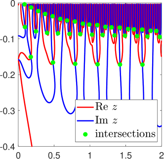
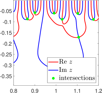
Figure 9: Internal method of numerically computing the resonances. Red curves are 0 level contours for the equation governing the real part of $z$, blue curves are for the imaginary part of $z$, and green dots are their intersections. The right graph is a zoomed-in version of the left, which corresponds to Example 4 case $c$.

%% Setup

clc; clear;

% Scale parameters
h = 1E-1;

x = [0, 2];
% x = [0.95, 1.05];
% x = [1.000, 1.002];
xPts = linspace(x(1), x(end), 500);

y = [-3*h, 0];
% y = [-10*h, 0];

% choose N by running exactly one of the three boxes below

%% N = 2

% Parameters
l = 6; C1 = 1; C2 = 1; b1 = 2.0; b2 = 2.0;

% Algebraic equation for z
zEqn = @(z) (2*i.*z - C1*h^b1).*(2*i.*z - C2*h^b2).*exp(-2*i*l.*z./h) ...
    - C1*C2*h^(b1+b2);

% Comparison to theory
yTheory = ((b1+b2)/(2*l))*h*log(h) + h/(2*l)*log(abs(C1*C2) ./ (4.*xPts.^2));

%% N = 3

% Parameters
C1 = 1; C2 = 1; C3 = 1;
% l1 = 4; l2 = 2; b1 = 0.5; b2 = 2.0; b3 = 2.0;
l1 = 4; l2 = 2; b1 = 0.5; b2 = 0.5; b3 = 2.0;

% Algebraic equation for z
zEqn = @(z) (2*i.*z - C1*h^b1).*(2*i.*z - C2*h^b2).*(2*i.*z ....
    - C3*h^b3).*exp(-2*i*(l1+l2).*z./h) ...
    - (C1*h^b1).*(C2*h^b2).*(2*i.*z - C3*h^b3).*exp(-2*i*(l2).*z./h) ...
    - (2*i.*z - C1*h^b1).*(C2*h^b2).*(C3*h^b3).*exp(-2*i*(l1).*z./h) ...
    - (C1*h^b1).*(2*i.*z + C2*h^b2).*(C3*h^b3);

% Comparison to theory
% yTheory = (((b1+b3)/2)/(l1+l2))*h*log(h) ...
%     + h/(2*(l1+l2))*log(abs(C1*C3) ./ (4.*xPts.^2)); % gamma 13
yTheory = ((b1+b2)/(2*l1))*h*log(h) ...
    + h/(2*l1)*log(abs(C1*C2) ./ (4.*xPts.^2)); % gamma 12
yTheory2 = ((b3-b2)/(2*l2))*h*log(h) ...
    + h/(2*l2)*log(abs(C3/C2)) .* ones(size(xPts)); % gamma 23

%% N = 4

% Parameters
C1 = 1; C2 = 1; C3 = 1; C4 = 1;
% l1 = 2; l2 = 3; l3 = 1; b1 = 2; b2 = 2; b3 = 2; b4 = 2; % gamma 14
% l1 = 2; l2 = 3; l3 = 1; b1 = 2; b2 = 2; b3 = .5; b4 = 2; % gamma 13, 34
l1 = 2; l2 = 3; l3 = 1; b1 = 2; b2 = .5; b3 = .5; b4 = 2; % gamma 23, 12, 34
% l1 = 3; l2 = 1; l3 = 2; b1 = .5; b2 = .5; b3 = 2; b4 = 3; % gamma 12, 24
% l1 = 3; l2 = 2; l3 = 1; b1 = .5; b2 = .5; b3 = 2; b4 = 3; % gamma 12, 23, 34
% l1 = 1; l2 = 3; l3 = 1; b1 = 2; b2 = .5; b3 = .5; b4 = 2; % double string
% l1 = 2; l2 = 3; l3 = 1; b1 = 1.5; b2 = .5; b3 = .5; b4 = 2; % crossed strings
% C1 = 10; C3 = -5; l1 = 2; l2 = 3; l3 = 1; b1 = 2; b2 = .5; b3 = .5; b4 = 2;

% Algebraic equation for z
R1 = @(z) (C1*h^b1)./(2*i.*z-C1*h^b1);
R2 = @(z) (C1*h^b2)./(2*i.*z-C2*h^b2);
R3 = @(z) (C1*h^b3)./(2*i.*z-C3*h^b3);
R4 = @(z) (C1*h^b4)./(2*i.*z-C4*h^b4);

zEqn = @(z) -exp(-2*i*(l1+l2+l3).*z./h) ...
    + R1(z).*R2(z).*exp(-2*i*(l2+l3).*z./h) ...
    + R2(z).*R3(z).*exp(-2*i*(l1+l3).*z./h) ...
    + R3(z).*R4(z).*exp(-2*i*(l1+l2).*z./h) ...
    + R2(z).*(1+2*R3(z)).*R4(z).*exp(-2*i*(l1).*z./h) ...
    - R1(z).*R2(z).*R3(z).*R4(z).*exp(-2*i*(l2).*z./h) ...
    + R1(z).*(1+2*R2(z)).*R3(z).*exp(-2*i*(l3).*z./h) ...
    + R1(z).*(1+2*R2(z)).*(1+2*R3(z)).*R4(z);

% Comparison to theory

% Dominant strings
% yTheory = ((b1+b2)/(2*l1))*h*log(h) ...
%     + h/(2*l1)*log(abs(C1*C2) ./ (4.*xPts.^2)); % gamma 12
yTheory = ((b2+b3)/(2*l2))*h*log(h) ...
    + h/(2*l2)*log(abs(C2*C3) ./ (4.*xPts.^2)); % gamma 23
% yTheory = ((b1+b3)/(2*(l1+l2)))*h*log(h) ...
%     + h/(2*(l1+l2))*log(abs(C1*C3)./ (4.*xPts.^2)); % gamma 13
% yTheory = ((b1+b4)/(2*(l1+l2+l3)))*h*log(h) ...
%     + h/(2*(l1+l2+l3))*log(abs(C1*C4) ./ (4.*xPts.^2)); % gamma 14

% Nondominant strings
% yTheory2 = ((b4-b2)/(2*(l2+l3)))*h*log(h) * ones(size(xPts)); % gamma 24
yTheory2 = ((b4-b3)/(2*l3))*h*log(h) * ones(size(xPts)); % gamma 34
% yTheory3 = ((b3-b2)/(2*(l2)))*h*log(h) * ones(size(xPts)); % gamma 23
yTheory3 = ((b1-b2)/(2*l1))*h*log(h) * ones(size(xPts)); % gamma 21

%% Compute contours and intersections

zReal = @(x, y) real(zEqn(x + i*y));
zImag = @(x, y) imag(zEqn(x + i*y));

% Compute 0 level contours of the real and imaginary part
mesh = 2500;
figure()
f = fcontour(zReal, [x(1) x(end) y(1) y(end)], ’LevelList’, 0, ’MeshDensity’, mesh);
Mreal = f.ContourLines.VertexData;
close;
figure()
f = fcontour(zImag, [x(1) x(end) y(1) y(end)], ’LevelList’, 0, ’MeshDensity’, mesh);
Mimag = f.ContourLines.VertexData;
close;

% Find the intersections of the above contours
% uses intersections() from Fast and Robust Curve Intersections by Douglas Schwarz
Mreal = Mreal(:,1:3:end); % uniformly remove data for speed
Mimag = Mimag(:,1:3:end);
epsilon = 0.03*h; % cutoff intersections within epsilon of domain
Mimag(1, abs(Mimag(1,:) - x(1)) < epsilon) = NaN;
Mimag(1, abs(Mimag(1,:) - x(end)) < epsilon) = NaN;
Mimag(2, abs(Mimag(2,:) - y(1)) < epsilon) = NaN;
Mimag(2, abs(Mimag(2,:) - y(end)) < epsilon) = NaN;
Mreal(1, abs(Mreal(1,:) - x(1)) < epsilon) = NaN;
Mreal(1, abs(Mreal(1,:) - x(end)) < epsilon) = NaN;
Mreal(2, abs(Mreal(2,:) - y(1)) < epsilon) = NaN;
Mreal(2, abs(Mreal(2,:) - y(end)) < epsilon) = NaN;
[resReal, resImag, iout, jout] = intersections(Mreal(1,:), Mreal(2,:), ...
    Mimag(1,:), Mimag(2,:), 0);

% Diagnostics: check the green dots are at the intersection of contours
figure()
hold on;
plot(Mreal(1, :), Mreal(2, :), ’.’, ’Color’, ’red’)
plot(Mimag(1, :), Mimag(2, :), ’.’, ’Color’, ’blue’)
plot(resReal, resImag, ’.’, ’Color’, ’green’, ’MarkerSize’, 20)
xlim(x);
ylim(y);

% Diagnostics: check a resonance is the root with << h^2 precision of the main equation
resIndex = 15;
fprintf("f(%.16f + %.16f*i) = %.1E + %.1E i\n", resReal(resIndex), resImag(resIndex), ...
    zReal(resReal(resIndex), resImag(resIndex)), zImag(resReal(resIndex), resImag(resIndex)))

%% Plotting

figure()
hold on; box on; pbaspect([1 1 1]);
set(gca, ’DefaultLineLineWidth’, 2, ’DefaultTextInterpreter’, ’latex’, ...
    ’fontsize’, 16);
plot(resReal, resImag, ’x’, ’Color’, ’red’, ’MarkerSize’, 10)
plot(xPts, yTheory, ’Color’, ’blue’);
plot(xPts, yTheory2, ’Color’, ’blue’);
plot(xPts, yTheory3, ’Color’, ’blue’);

xlim(x);
ylim([-0.3,0]);
legend("resonances", "theorem 2", "location", "southeast", "Interpreter", "latex", ...
    ’fontsize’, 20)

10 Acknowledgements

I would like to deeply thank Professor Kiril Datchev for his ample guidance, introduction to the problem, and thorough edits. I would also like to thank Professors Jared Wunsch and Jeremy Marzuola for insightful discussions. This research was conducted at Purdue University.

Division of Applied Mathematics, Brown University, Providence, RI 02906

E-mail address: ethan_brady@brown.edu

References

• [1] Matthew C. Barr, Michael P. Zaletel and Eric J. Heller “Quantum corral resonance widths: lossy scattering as acoustics” In NANO LETTERS 10.9, 2010, pp. 3253–3260 DOI: 10.1021/nl100569w
• [2] M. Belloni and R.. Robinett “The infinite well and Dirac delta function potentials as pedagogical, mathematical and physical models in quantum mechanics” In PHYSICS REPORTS-REVIEW SECTION OF PHYSICS LETTERS 540.2, 2014, pp. 25–122 DOI: 10.1016/j.physrep.2014.02.005
• [3] N Burq “Poles of scattering engendered by a corner” In ASTERISQUE, 1997, pp. 3+
• [4] Kiril Datchev and Nkhalo Malawo “Semiclassical resonance asymptotics for the delta potential on the half line” In PROCEEDINGS OF THE AMERICAN MATHEMATICAL SOCIETY 150.11, 2022, pp. 4909–4921 DOI: 10.1090/proc/16001
• [5] Kiril Datchev, Jeremy L. Marzuola and Jared Wunsch “Newton polygons and resonances of multiple delta-potentials” In Transactions of the American Mathematical Society, 2023 DOI: 10.1090/tran/9056
• [6] Semyon Dyatlov and Maciej Zworski “Mathematical theory of scattering resonances” AMERICAN MATHEMATICAL SOCIETY, 2019
• [7] Fatih Erman, Manuel Gadella and Haydar Uncu “On scattering from the one-dimensional multiple Dirac delta potentials” In EUROPEAN JOURNAL OF PHYSICS 39.3, 2018 DOI: 10.1088/1361-6404/aaa8a3
• [8] Fatih Erman, Manuel Gadella, Secil Tunali and Haydar Uncu “A singular one-dimensional bound state problem and its degeneracies” In EUROPEAN PHYSICAL JOURNAL PLUS 132.8, 2017 DOI: 10.1140/epjp/i2017-11613-7
• [9] Jeffrey Galkowski “Distribution of resonances in scattering by thin barriers” In MEMOIRS OF THE AMERICAN MATHEMATICAL SOCIETY 259.1248, 2019, pp. 1+ DOI: 10.1090/memo/1248
• [10] David J. Griffiths “Introduction to Quantum Mechanics” Prentice Hall, 1995
• [11] Luc Hillairet and Jared Wunsch “On resonances generated by conic diffraction” In ANNALES DE L INSTITUT FOURIER 70.4, 2020, pp. 1715–1752
• [12] Basudeb Sahu and Bidhubhusan Sahu “Accurate delta potential approximation for a coordinate-dependent potential and its analytical solution” In PHYSICS LETTERS A 373.44, 2009, pp. 4033–4037 DOI: 10.1016/j.physleta.2009.09.018
• [13] Douglas Schwarz “Fast and Robust Curve Intersections” MATLAB Central File Exchange, 2023 URL: https://www.mathworks.com/matlabcentral/fileexchange/11837-fast-and-robust-curve-intersections
• [14] A. Tanimu and E.. Muljarov “Resonant states in double and triple quantum wells” In JOURNAL OF PHYSICS COMMUNICATIONS 2.11, 2018 DOI: 10.1088/2399-6528/aae86a
• [15] M Zworski “Distribution of poles for scattering on the real line” In JOURNAL OF FUNCTIONAL ANALYSIS 73.2, 1987, pp. 277–296 DOI: 10.1016/0022-1236(87)90069-3