Chaotic properties of billiards in circular polygons

Abstract

We study billiards in domains enclosed by circular polygons. These are closed $C^{1}$ strictly convex curves formed by finitely many circular arcs. We prove the existence of a set in phase space, corresponding to generic sliding trajectories close enough to the boundary of the domain, in which the return billiard dynamics is semiconjugate to a transitive subshift on infinitely many symbols that contains the full $N$-shift as a topological factor for any $N\in\mathbb{N}$, so it has infinite topological entropy. We prove the existence of uncountably many asymptotic generic sliding trajectories approaching the boundary with optimal uniform linear speed, give an explicit exponentially big (in $q$) lower bound on the number of $q$-periodic trajectories as $q\to\infty$, and present an unusual property of the length spectrum. Our proofs are entirely analytical.

Keywords: Billiards, circular polygons, symbolic dynamics, periodic trajectories, length spectrum

1 Introduction

A billiard problem concerns the motion of a particle inside the domain bounded by a closed plane curve $\Gamma$ (or the domain bounded by a hypersurface of some higher-dimensional Euclidean space). The motion in the interior of the domain is along straight lines, with elastic collisions at the boundary according to the optical law of reflection: the angles of incidence and reflection are equal. These dynamical systems were first introduced by Birkhoff [9]. See [41, 57, 18] for a general description.

In the case of dispersing billiards (i.e. when the boundary is a union of concave components), the dynamics is chaotic [55]; indeed, such billiards exhibit ergodicity, the Bernoulli property, sensitive dependence on initial conditions, and so forth. In fact, it was believed for some years that billiards without any dispersing walls could not display chaos.

Thus it came as a surprise when Bunimovich, in his famous paper, detailed a proof that the billiard in a stadium exhibits the Bernoulli property [12]. The boundary of the stadium billiard consists of two straight parallel lines connected at either end by semicircles. Stadia are $C^{1}$ and convex, but not $C^{2}$ or strictly convex. We study the class of $C^{1}$ strictly convex billiards bounded by finitely many circular arcs. No billiard in this class satisfies the celebrated B-condition—that is, all circular arcs can be completed to a disk within the billiard domain—, which is the hallmark for the defocusing mechanism in billiards whose focusing boundaries are all circular arcs [18, Section 8.3]. In spite of it, we observe several chaotic phenomena.

A closed curve $\Gamma$ in $\mathbb{R}^{2}$ is called a circular polygon if it is a union of a finite number of circular arcs such that $\Gamma$ is $C^{1}$ and strictly convex. We do not consider circumferences as circular polygons. A circular $k$-gon is a circular polygon with exactly $k$ arcs. If $\Gamma$ is a circular $k$-gon, then $k\geq 4$. The phase space $\mathcal{M}$ is a 2-dimensional cylinder; the circular component of the cylinder is a parameter on the curve $\Gamma$, and the height component is the angle of incidence/reflection. We denote by $f:\mathcal{M}\to\mathcal{M}$ the billiard map (i.e. the collision map of the billiard flow with the boundary $\Gamma$ of the domain; see Section 4 for a precise definition). In what follows we give heuristic statements of our main results.

Theorem A.

If $\Gamma$ is a circular polygon, then there is a set $\mathcal{J}\subset\mathcal{M}$ accumulating on $\partial\mathcal{M}$ such that the return map $F:\mathcal{J}\to\mathcal{J}$ of $f$ to $\mathcal{J}$ is topologically semiconjugate to a transitive subshift on infinitely many symbols that contains the full $N$-shift as a topological factor for any $N\in\mathbb{N}$, so it has infinite topological entropy.

See Proposition 27 in Section 5 and Theorem 31 in Section 6 for a precise formulation of this theorem. Be aware that the map with infinite entropy is the return map $F$, not the billiard map $f$.

The final sliding motions are the possible qualitative behaviors that a sliding billiard trajectory posses as the number of impacts tends to infinity, forward or backward. Every forward counter-clockwise sliding billiard trajectory $(\varphi_{n},\theta_{n})=f^{n}(\varphi,\theta)$, where $\varphi_{n}$ are the angles of impact and $\theta_{n}$ are the angles of incidence/reflection, belongs to exactly one of the following three classes:

• Forward bounded ($\mathcal{B}_{0}^{+}$): $\inf_{n\geq 0}\theta_{n}>0$;

• Forward oscillatory ($\mathcal{O}_{0}^{+}$): $0=\liminf_{n\to+\infty}\theta_{n}<\limsup_{n\to+\infty}\theta_{n}$; and

• Forward asymptotic ($\mathcal{A}_{0}^{+}$): $\lim_{n\to+\infty}\theta_{n}=0$.

This classification also applies for backward counter-clockwise sliding trajectories when $n\leq-1$ and $n\to-\infty$, in which case we write a superindex $-$ instead of $+$ in each of the classes: $\mathcal{B}_{0}^{-}$, $\mathcal{O}_{0}^{-}$ and $\mathcal{A}_{0}^{-}$. And it also applies to (backward or forward) clockwise sliding trajectories, in which case we replace $\theta_{n}$ with $|\theta_{n}-\pi|$ in the definitions above and we write a subindex $\pi$ instead of $0$ in each of the classes: $\mathcal{B}_{\pi}^{\pm}$, $\mathcal{O}_{\pi}^{\pm}$ and $\mathcal{A}_{\pi}^{\pm}$.

Terminologies bounded and oscillatory are borrowed from Celestial Mechanics. See, for instance, [32]. In our billiard setting, bounded means bounded away from $\theta=\pi$ in the clockwise case and bounded away from $\theta=0$ in the counter-clockwise case. That is, a sliding billiard trajectory is bounded when it does not approach $\partial\mathcal{M}$.

The following corollary is an immediate consequence of Theorem A, see Section 6.

Corollary B.

If $\Gamma$ is a circular polygon, then $\mathcal{X}_{\lambda}^{-}\cap\mathcal{Y}_{\lambda}^{+}\neq\emptyset$ for $\mathcal{X},\mathcal{Y}\in\{\mathcal{B},\mathcal{O},\mathcal{A}\}$ and $\lambda\in\{0,\pi\}$.

From now on, we focus on counter-clockwise sliding trajectories. Corollary B does not provide data regarding the maximal speed of diffusion for asymptotic trajectories. Which is the faster way in which $\theta_{n}\to 0$ for asymptotic sliding trajectories? The answer is provided in the following theorem.

Theorem C.

If $\Gamma$ is a circular polygon, then there are uncountably many asymptotic generic sliding billiard trajectories that approach the boundary with uniform linear speed. That is, there are constants $0<a<b$ such that if $\{\theta_{n}\}_{n\in\mathbb{Z}}$ is the corresponding sequence of angles of incidence/reflection of any of these uncountably many asymptotic generic sliding billiard trajectories, then

$$a|n|\leq 1/\theta_{n}\leq b|n|,\qquad\forall|n|\gg 1.$$

Linear speed is optimal. That is, there is no billiard trajectory such that

$$\lim_{n\to+\infty}n\theta_{n}=0.$$

See Theorem 35 in Section 7, where we also get uncountably many one-parameter families (paths) of forward asymptotic generic sliding billiard trajectories, for a more detailed version of Theorem C. The term sliding in Theorem C means that our trajectories do not skip any arc in any of their infinite turns around $\Gamma$. The definition of generic billiard trajectories is a bit technical, see Definition 13 and Remark 14. The term uniform means that constants $0<a<b$ do not depend on the billiard trajectory. The term linear means that $1/\theta_{n}$ is bounded between two positive multiples of $|n|$. Optimality comes as a no surprise since $\sum_{n\geq 0}\theta_{n}=+\infty$ for any billiard trajectory in any circular polygon—or, for that matter, in any strictly convex billiard table whose billiard flow is defined for all time [33]. Optimality is proved in Proposition 36 in Section 7.

There are two key insights (see Section 4) behind this theorem. First, when we iterate $f$ along one of the circular arcs of the circular polygon $\Gamma$, the angle of reflection $\theta$ is constant, so $\theta$ can drop only when the trajectory crosses the singularities between consecutive circular arcs. Second, the maximal drop corresponds to multiply $\theta$ by an uniform (in $\theta$) factor smaller than one. As we must iterate the map many (order $\theta^{-1}$) times to fully slide along each circular arc, we can not approach the boundary with a faster than linear speed.

As Theorem A gives us only a topological semiconjugacy to symbolic dynamics, it does not immediately provide us with the abundance of periodic orbits that the shift map possesses. However our techniques enable us to find many periodic sliding billiard trajectories. We state in the following theorem that the number of such trajectories in circular polygons grows exponentially with respect to the period. In contrast, Katok [38] showed that the numbers of isolated periodic billiard trajectories and of parallel periodic billiard trajectories grow subexponentially in any (linear) polygon.

Given any integers $1\leq p<q$, let $\Pi(p,q)$ be the set of $(p,q)$-periodic billiard trajectories in $\Gamma$. That is, the set of periodic trajectories that close after $p$ turns around $\Gamma$ and $q$ impacts in $\Gamma$, so they have rotation number $p/q$. Let $\Pi(q)=\cup_{1\leq p<q}\Pi(p,q)$ be the set of periodic billiard trajectories with period $q$. The symbol $\#$ denotes the cardinality of a set.

Theorem D.

If $\Gamma$ is a circular $k$-gon and $p\in\mathbb{N}$, there are constants $c_{\star}(p),M_{\star},h_{\star}>0$ such that

1. $\#\Pi(p,q)\geq c_{\star}(p)q^{kp-1}+\mathop{\rm O}\nolimits(q^{kp-2})$ as $q\to\infty$ for any fixed $p\in\mathbb{N}$; and

2. $\#\Pi(q)\geq M_{\star}{\rm e}^{h_{\star}q}/q$ as $q\to+\infty$.

We give explicit expressions for $c_{\star}(p)$, $M_{\star}$ and $h_{\star}$ in Section 8. The optimal value of $c_{\star}(p)$ is equal to the volume of certain $(kp-1)$-dimensional compact convex polytope with an explicitly known half-space representation, see Proposition 39. We do not give optimal values of $M_{\star}$ and $h_{\star}$. The relation between the optimal value of $h_{\star}$ and the topological entropy of the billiard map $f$ is an open problem. We acknowledge that some periodic trajectories in $\Pi(p,q)$ may have period less that $q$ when $\gcd(p,q)\neq 1$, but they are a minority, so the previous lower bounds captures the growth rate of the number of periodic trajectories with rotation number $p/q$ and minimal period $q$ even when $p$ and $q$ are not coprime.

If the circular billiard has some symmetry, we can perform the corresponding natural reduction to count the number of symmetric sliding periodic trajectories, but then the exponent $kp-1$ in the first lower bound would be smaller because there are less reduced arcs than original arcs. Exponent $h_{\star}$ would be smaller too. See [16, 28] for samples of symmetric periodic trajectories in other billiards. The first reference deals with axial symmetries. The second one deals with rotational symmetries.

Let $|\Gamma|$ be the length of $\Gamma$. If $g=\{z_{0},\ldots,z_{q-1}\}\subset\Gamma$ is a $q$-periodic billiard trajectory, let $L(g)=|z_{1}-z_{0}|+\cdots+|z_{q-1}-z_{0}|$ be its length. If $(g_{q})_{q}$ is any sequence such that $g_{q}\in\Pi(1,q)$, then $\lim_{q\to+\infty}L(g_{q})=|\Gamma|$. There are so many generic sliding $(1,q)$-periodic billiard trajectories inside circular polygons that we can find sequences $(g_{q})_{q}$ such that the differences $L(g_{q})-|\Gamma|$ have rather different asymptotic behaviors as $q\to+\infty$.

Theorem E.

If $\Gamma$ is a circular polygon, then there are constants $c_{-}<c_{+}<0$ such that for any fixed $c\in[c_{-},c_{+}]$ there exist a sequence $(g_{q})_{q}$, with $g_{q}\in\Pi(1,q)$, such that

$$L(g_{q})=|\Gamma|+c/q^{2}+\mathop{\rm O}\nolimits(1/q^{3}),\quad\mbox{as $q\to+\infty$.}$$

Consequently, there exist a sequence $(h_{q})_{q}$, with $h_{q}\in\Pi(1,q)$, such that

$$c_{-}=\liminf_{q\to+\infty}\big{(}(L(h_{q})-|\Gamma|)q^{2}\big{)}<\limsup_{q\to+\infty}\big{(}(L(h_{q})-|\Gamma|)q^{2}\big{)}=c_{+},\quad\mbox{as $q\to+\infty$.}$$

Besides, $c_{-}\leq-\pi^{2}|\Gamma|/6$ and $c_{+}=-\frac{1}{24}\left[\int_{\Gamma}\kappa^{2/3}(s)\,{\rm d}s\right]^{3}$, where $\kappa(s)$ is the curvature of $\Gamma$ as a function of an arc-length parameter $s\in[0,|\Gamma|)$.

Let us put these results into perspective by comparing them with the observed behavior in sufficiently smooth (say $C^{6}$) and strictly convex billiards, which for the purpose of this discussion we refer to as Birkhoff billiards. Lazutkin’s theorem (together with a refinement due to Douady) implies that Birkhoff billiards possess a family of caustics accumulating on the boundary [23, 42]. These caustics divide the phase space into invariant regions, and therefore guarantee a certain regularity of the dynamics near the boundary, in the sense that the conclusion of Theorem A never holds for Birkhoff billiards. Not only does the conclusion of Theorem C not hold for Birkhoff billiards, but in such systems there are no trajectories approaching the boundary asymptotically as the orbits remain in invariant regions bounded by the caustics. As for Theorem D, a well-known result of Birkhoff [9] implies that Birkhoff billiards have $\#\Pi(p,q)\geq 2$ for each coprime pair $p,q$ such that $1\leq p<q$. This lower bound turns out to be sharp, in the sense that for any such pair $p,q$, there exist Birkhoff billiards with exactly two geometrically distinct periodic orbits of rotation number $p/q$ [51]; a simple example is that the billiard in a non-circular ellipse has two periodic orbits of rotation number $1/2$, corresponding to the two axes of symmetry. It follows that the conclusion of Theorem D does not hold in general for Birkhoff billiards. Finally, as for Theorem E, a well-known result of Marvizi-Melrose [45] implies that if $(g_{q})_{q}$, with $g_{q}\in\Pi(1,q)$, is any sequence of periodic billiard trajectories in a Birkhoff billiard $\Gamma$, then

$$L(g_{q})=|\Gamma|+c_{+}/q^{2}+\mathop{\rm O}\nolimits(1/q^{4}),\quad\mbox{as $q\to+\infty$,}$$

where $c_{+}=-\frac{1}{24}\left[\int_{\Gamma}\kappa^{2/3}(s)\,{\rm d}s\right]^{3}$. Hence, $(1,q)$-periodic billiard trajectories in circular polygons are asymptotically shorter than the ones in Birkhoff billiards.

An interesting question in general that has been considered to a significant extent in the literature is: what happens to the caustics of Lazutkin’s theorem, and thus the conclusions of Theorems A and C, if we loosen the definition of a Birkhoff billiard? Without altering the basic definition of the billiard map $f$, there are three ways that we can generalize Birkhoff billiards: (i) by relaxing the strict convexity hypothesis, (ii) by relaxing the smoothness hypothesis, or (iii) by increasing the dimension of the ambient Euclidean space.

1. Mather proved that if the boundary is convex and $C^{r}$ for $r\geq 2$, but has at least one point of zero curvature, then there are no caustics and there exist trajectories which come arbitrarily close to being positively tangent to the boundary and also come arbitrarily close to being negatively tangent to the boundary [46]. Although this result is about finite segments of billiard trajectories, there are also infinite trajectories tending to the boundary both forward and backward in time in such billiards: $\mathcal{A}_{0}^{\pm}\cap\mathcal{A_{\pi}^{\mp}}\neq\emptyset$, see [47].

2. Despite six continuous derivatives being the standard smoothness requirement for Lazutkin’s theorem [23, 42], there is some uncertainty regarding what happens for $C^{5}$ boundaries, and in fact it is generally believed that 4 continuous derivatives should suffice. Halpern constructed billiard tables that are strictly convex and $C^{1}$ but not $C^{2}$ such that the billiard particle experiences an infinite number of collisions in finite time [33]; that is to say, the billiard flow is incomplete. This construction does not apply to our case, as our billiard boundaries have only a finite number of singularities (points where the boundary is only $C^{1}$ and not $C^{2}$), whereas Halpern’s billiards have infinitely many.

   The case of boundaries that are strictly convex and $C^{1}$ but not $C^{2}$ and have only a finite number (one, for example) of singularities was first considered by Hubacher [36], who proved that such billiards have no caustics in a neighborhood of the boundary. This result opens the door for our analysis.

3. It has been known since the works of Berger and Gruber that in the case of strictly convex and sufficiently smooth billiards in higher dimension (i.e. the billiard boundary is a codimension 1 submanifold of $\mathbb{R}^{d}$ where $d\geq 3$), only ellipsoids have caustics [7, 30]. However Gruber also observed that in this case, even in the absence of caustics, the Liouville measure of the set of trajectories approaching the boundary asymptotically is zero [29]. The question of existence of such trajectories was thus left open.

   It was proved in [20] (combined with results of [19]) that generic strictly convex analytic billiards in $\mathbb{R}^{3}$ (and ‘many’ such billiards in $\mathbb{R}^{d}$ for $d\geq 4$) have trajectories approaching the boundary asymptotically. It is believed that the meagre set of analytic strictly convex billiard boundaries in $\mathbb{R}^{d}$, $d\geq 3$, for which these trajectories do not exist consists entirely of ellipsoids, but the perturbative methods of [20] do not immediately extend to such a result.

Billiards in circular polygons have been studied numerically in the literature [6, 24, 34, 35, 44]. In the paper [4] the authors use numerical simulations and semi-rigorous arguments to study billiards in a 2-parameter family of circular polygons. They conjecture that, for certain values of the parameters, the billiard is ergodic. In addition they provide heuristic arguments in favor of this conjecture.

A related problem is the lemon-shaped billiard, which is known to display chaos [11, 17, 37]. These billiards are strictly convex but not $C^{1}$, so the billiard map is well-defined only on a proper subset of the phase space.

The elliptic flowers recently introduced by Bunimovich [13] are closed $C^{0}$ curves formed by finitely many pieces of ellipses. Elliptic polygons are elliptic flowers that are $C^{1}$ and strictly convex, so they are a natural generalization of circular polygons. One can obtain a 1-parameter family of elliptic polygons with the string construction from any convex (linear) polygon. The string construction consists of wrapping an inelastic string around the polygon and tracing a curve around it by keeping the string taut. Billiards in elliptic polygons can be studied with the techniques presented here for circular polygons. We believe that all results previously stated in this introduction, with the possible exception of inequality $c_{-}\leq-\pi^{2}|\Gamma|/6$ given in Theorem E, hold for generic elliptic polygons. However, there are elliptic polygons that are globally $C^{2}$, and not just $C^{1}$, being the hexagonal string billiard first studied by Fetter [25] the most celebrated example. We do not know how to deal with $C^{2}$ elliptic polygons because jumps in the curvature of the boundary are a key ingredient in our approach to get chaotic billiard dynamics. Fetter suggested that the hexagonal string billiard could be integrable, in which case it would be a counterexample to the Birkhoff conjecture. However, such integrability was numerically put in doubt in [8]. Later on is was analytically proved that a string billiard generated from a convex polygon with a least three sides can not have caustics near the boundary [14].

In what follows we describe the main ideas of our proofs. Let $\Gamma$ be a circular $k$-gon. It is well-known that the angle of incidence/reflection is a constant of motion for billiards in circles. Therefore, for the billiard in $\Gamma$, the angle of incidence/reflection can change only when we pass from one circular arc to another, and not when the billiard has consecutive impacts on the same circular arc. The main tool that we use to prove our theorems is what we call the fundamental lemma (Lemma 18 below), which describes how trajectories move up and down after passing from one circular arc to the next. The phase space $\mathcal{M}$ of the billiard map $f$ is a cylinder, with coordinates $(\varphi,\theta)$ where $\varphi\in\mathbb{T}$ is a parameter on the boundary $\Gamma$, and where $\theta\in[0,\pi]$ is the angle of incidence/reflection. We consider two vertical segments $\mathcal{L}_{j}$ and $\mathcal{L}_{j+1}$ in $\mathcal{M}$ corresponding to consecutive singularities of $\Gamma$, and sufficiently small values of $\theta$. The index $j$ that labels the singularities is defined modulo $k$. The triangular region $\mathcal{D}_{j}$ bounded by $\mathcal{L}_{j}$ and $f(\mathcal{L}_{j})$ is a fundamental domain of the billiard map $f$; that is, a set with the property that sliding trajectories have exactly one point in $\mathcal{D}_{j}$ on each turn around $\Gamma$. Consider now the sequence of backward iterates $\big{\{}f^{-n}(\mathcal{L}_{j+1})\big{\}}$ of $\mathcal{L}_{j+1}$. This sequence of slanted segments divides the fundamental domain $\mathcal{D}_{j}$ into infinitely many quadrilaterals, which we call fundamental quadrilaterals. The fundamental lemma describes which fundamental quadrilaterals in $\mathcal{D}_{j+1}$ we can visit if we start in a given fundamental quadrilateral in $\mathcal{D}_{j}$.

In order to prove Theorem A, we apply the fundamental lemma iteratively to describe how trajectories visit different fundamental quadrilaterals consecutively in each of the $k$ fundamental domains $\mathcal{D}_{j}$ in $\mathcal{M}$. A particular coding of possible sequences of $k$ fundamental quadrilaterals that trajectories can visit gives us our symbols. We then use a method due to Papini and Zanolin [49, 50] (extended to higher dimensions by Pireddu and Zanolin [52, 53, 54]) to prove that the billiard dynamics is semiconjugate to a shift map on the sequence space of this set of symbols; this method is called stretching along the paths. Observe that we could equally have used the method of correctly aligned windows [3, 27, 59], or the crossing number method [40]; note however that the latter would not have provided us with the large amount of periodic orbits that the other two methods do. We note that, although Theorem A provides us with a topological semiconjugacy to symbolic dynamics, we expect that this could be improved to a full conjugacy by using other methods.

Once the proof of Theorem A is completed, Theorems C, D, and E are proved by combining additional arguments with the symbolic dynamics we have constructed. With respect to the symbolic dynamics, we choose a coding of the fundamental quadrilaterals visited by a trajectory that corresponds to $\theta$ tending to $0$ in the fastest way possible. We then prove that the corresponding billiard trajectories satisfy the conclusion of Theorem C. As for Theorem D, the method of stretching along the paths guarantees the existence of a periodic billiard trajectory for every periodic sequence of symbols. Consequently, the proof of Theorem D amounts to counting the number of sequences of symbols that are periodic with period $p$ (because each symbol describes one full turn around the table; see Section 5 for details) such that the corresponding periodic sliding billiard trajectories after $p$ turns around the table have rotation number $p/q$. It turns out that this reduces to counting the number of integer points whose coordinates sum $q$ in a certain $kp$-dimensional convex polytope. We do this by proving that the given convex polytope contains a hypercube with sides of a certain length, and finally by counting the number of integer points whose coordinates sum $q$ in that hypercube.

The structure of this paper is as follows. In Section 2 we describe the salient features of circular polygons. We summarize the stretching along the paths method in Section 3. Section 4 is concerned with the definition of fundamental quadrilaterals, as well as the statement and proof of the fundamental lemma. Symbols are described in Section 5. Chaotic dynamics, and thus the proofs of Theorem A and Corollary B, is established in Section 6, whereas Section 7 contains the proof of Theorem C. In Section 8, we count the periodic orbits, thus proving Theorem D. Finally, Theorem E is proved in Section 9. Some technical proofs are relegated to appendices.

2 Circular polygons

In this section we define our relevant curves, construct their suitable parametrisations, and introduce notations that will be extensively used in the rest of the paper.

A piecewise-circular curve (or PC curve for short) is given by a finite sequence of circular arcs in the Euclidean plane $\mathbb{R}^{2}$, with the endpoint of one arc coinciding with the beginning point of the next. PC curves have been studied by several authors. See [5, 15] and the references therein. Lunes and lemons (two arcs), yin-yang curves, arbelos and PC cardioids (three arcs), salinons, Moss’s eggs and pseudo-ellipses (four arcs), and Reuleaux polygons (arbitrary number of arcs) are celebrated examples of simple closed PC curves [22, 1]. A simple closed PC curve is a PC curve not crossing itself such that the endpoint of its last arc coincides with the beginning point of its first arc.

All simple closed PC curves are Jordan curves, so we could study the billiard dynamics in any domain enclosed by a simple closed PC curve. However, such domains are too general for our purposes. We will only deal with strictly convex domains without corners or cusps. Strict convexity is useful, because then any ordered pair of points on the boundary defines a unique billiard trajectory. Absence of cusps and corners implies that the corresponding billiard map is a global homeomorphism in the phase space $\mathcal{M}$, see Section 4.

Therefore, we will only consider circular polygons, defined as follows.

Definition 1.

A circular $k$-gon is a simple closed strictly convex curve in $\mathbb{R}^{2}$ formed by the concatenation of $k>1$ circular arcs, in such a way that the curve is $C^{1}$, but not $C^{2}$, at the intersection points of any two consecutive circular arcs. The nodes of a circular polygon are the intersection points of each pair of consecutive circular arcs.

Reuleaux polygons, lemons, lunes, yin-yang curves, arbelos, salinons, PC cardioids are not circular polygons, but pseudo-ellipses and Moss’s eggs (described later on; see also [22, Section 1.1]) are. We explicitly ask that consecutive arcs always have different radii, so the curvature has jump discontinuities at all nodes. We do not consider circumferences as circular polygons since circular billiards are completely integrable.

Let $\Gamma$ be a circular $k$-gon with arcs $\Gamma_{1},\ldots,\Gamma_{k}$, listed in the order in which they are concatenated, moving in a counter-clockwise direction. Each arc $\Gamma_{j}$ is completely determined by its center $O_{j}$, its radius $r_{j}>0$ and its angular range $[a_{j},b_{j}]\subset\mathbb{T}$. Then $\delta_{j}=b_{j}-a_{j}$ is the central angle of $\Gamma_{j}$. Using the standard identification $\mathbb{R}^{2}\simeq\mathbb{C}$, let

$$A_{j}=O_{j}+r_{j}{\rm e}^{\mskip 2.0mu{\rm i}\mskip 1.0mua_{j}},\qquad B_{j}=O_{j}+r_{j}{\rm e}^{\mskip 2.0mu{\rm i}\mskip 1.0mub_{j}}$$

be the two nodes of arc $\Gamma_{j}$. We denote by

$$\Gamma_{\star}=\{A_{1},\ldots,A_{k}\}=\{B_{1},\ldots,B_{k}\}$$ (1)

the set of nodes of $\Gamma$.

Notation 2.

The index $j$ that labels the arcs of any circular $k$-gon is defined modulo $k$. Hence, $\Gamma_{j}=\Gamma_{j\mod k}$, $r_{j}=r_{j\mod k}$, $a_{j}=a_{j\mod k}$ and so forth. In particular, $\Gamma_{k+1}=\Gamma_{1}$.

Definition 3.

The polar parametrisation of $\Gamma$ is the counter-clockwise parametrisation

$$z:\mathbb{T}\to\Gamma\subset\mathbb{R}^{2}\simeq\mathbb{C},\qquad z(\varphi)=O_{j}+r_{j}{\rm e}^{\mskip 2.0mu{\rm i}\mskip 1.0mu\varphi},\qquad\forall\varphi\in[a_{j},b_{j}].$$

The points $a_{1},\ldots,a_{k}$ are the singularities of $\Gamma$.

This parametrisation is well-defined because, by definition, $B_{j}=A_{j+1}$ (the endpoint of any arc coincides with the beginning point of the next), and $b_{j}=a_{j+1}$ (two consecutive arcs have the same oriented tangent line at their intersecting node). From now on, the reader should keep in mind that singularities $a_{1},\ldots,a_{k}$ are always ordered in such a way that

$$a_{1}<b_{1}=a_{2}<b_{2}=a_{3}<\cdots<b_{k-1}=a_{k}<b_{k}=a_{1}+2\pi.$$ (2)

As far as we know, all the billiards in circular polygons that have been studied in the past correspond to cases with exactly four arcs [4, 6, 24, 34, 35, 44]. It turns out that this is the simplest case, in the context of the next lemma.

Lemma 4.

Let $\Gamma$ be a circular $k$-gon with radii $r_{j}>0$, singularities $a_{j}\in\mathbb{T}$ (or $b_{j}=a_{j+1}$) and central angles $\delta_{j}=b_{j}-a_{j}\in(0,2\pi)$ for $j\mod k$. Set $w_{j}={\rm e}^{\mskip 2.0mu{\rm i}\mskip 1.0mub_{j}}-{\rm e}^{\mskip 2.0mu{\rm i}\mskip 1.0mua_{j}}\in\mathbb{C}$. Then $\Gamma$ has at least four arcs: $k\geq 4$, and

$$\sum_{j=1}^{k}\delta_{j}=2\pi,\qquad\sum_{j=1}^{k}r_{j}w_{j}=0.$$ (3)

Proof.

Clearly, $\sum_{j=1}^{k}\delta_{j}=\sum_{j=1}^{k}(b_{j}-a_{j})=b_{k}-a_{1}=2\pi$. It is known that a bounded measurable function $\rho\in L(\mathbb{T})$ is the radius of curvature of a closed curve if and only if

$$\int_{a_{1}}^{b_{k}}\rho(\varphi){\rm e}^{\mskip 2.0mu{\rm i}\mskip 1.0mu\varphi}\,{\rm d}\varphi=\int_{0}^{2\pi}\rho(\varphi){\rm e}^{\mskip 2.0mu{\rm i}\mskip 1.0mu\varphi}\,{\rm d}\varphi=0.$$ (4)

Since the radius of curvature of $\Gamma$ is the piecewise constant function $\rho_{|(a_{j},b_{j})}\equiv r_{j}$, the general condition (4) becomes $-\mskip 2.0mu{\rm i}\mskip 1.0mu\sum_{j=1}^{k}r_{j}w_{j}=0$. Note that $\sum_{j=1}^{k}w_{j}=0$, $w_{j}\neq 0$ for all $j$, and $\dim_{\mathbb{R}}[w_{1},\ldots,w_{k}]=2$ when $k\geq 3$. If $\Gamma$ has just two arcs: $k=2$, then

$$r_{1}w_{1}+r_{2}w_{2}=0,\qquad w_{1}+w_{2}=0,\qquad w_{1},w_{2}\neq 0.$$

This implies that $r_{1}=r_{2}$ and contradicts our assumption about radii of consecutive arcs. If $\Gamma$ has just three arcs: $k=3$, then

$$r_{1}w_{1}+r_{2}w_{2}+r_{3}w_{3}=0,\qquad w_{1}+w_{2}+w_{3}=0,\qquad\dim_{\mathbb{R}}[w_{1},w_{2},w_{3}]=2.$$

This implies that $r_{1}=r_{2}=r_{3}$ and we reach the same contradiction. ∎

Necessary conditions (2) and (3) are sufficient ones too. To be precise, if the radii $r_{j}>0$, the angular ranges $[a_{j},b_{j}]\subset\mathbb{T}$ and the central angles $\delta_{j}=b_{j}-a_{j}\in(0,2\pi)$ satisfy (2) and (3), then there exists a $2$-parameter family of circular $k$-gons sharing all those elements. To be precise, all circular $k$-gons in this family are the same modulo translations. Let us prove this claim. Once we put the center $O_{1}$ at an arbitrary location, all other centers are recursively determined by imposing that $A_{j+1}=B_{j}$, which implies (since $b_{j}=a_{j+1}$) that

$$O_{j+1}=O_{j}+(r_{j}-r_{j+1}){\rm e}^{\mskip 2.0mu{\rm i}\mskip 1.0mub_{j}},\qquad j=1,\ldots,k-1.$$

The obtained PC curve $\Gamma=z(\mathbb{T})$, where $z(\varphi)$ is the polar parametrisation introduced in Definition 3, is closed by (4) and it is $C^{1}$ and strictly convex by construction. Hence, $\Gamma$ is a circular $k$-gon. This means that any circular $k$-gon is completely determined once we know its first center $O_{1}$, its first singularity $a_{1}$, its radii $r_{1},\ldots,r_{k}$, and its central angles $\delta_{1},\ldots,\delta_{k}$.

The above discussion shows that circular $k$-gons form, modulo traslations and rotations, a $(2k-3)$-parameter family. To be precise, if we set $O_{1}=(0,0)$ and $a_{1}=0$ by means of a traslation and a rotation, then parameters $r_{1},\ldots,r_{k},\delta_{1},\ldots,\delta_{k}$ are restricted by (3), which has codimension three. If, in addition, we normalize somehow (in the literature one can find many different choices) our circular $k$-gons with a scaling, we get that they form a $(2k-4)$-parameter family modulo similarities. The reader can find a complete geometric description, modulo similarities, of the four-parameter family of (convex and nonconvex, symmetric and nonsymmetric) closed $C^{1}$ PC curves with four arcs in [34], whose goal was to numerically exhibit the richness of the billiard dynamics in those $C^{1}$ PC curves.

For brevity, we only give a few simple examples of symmetric and non-symmetric circular polygons with four and six arcs. We skip many details.

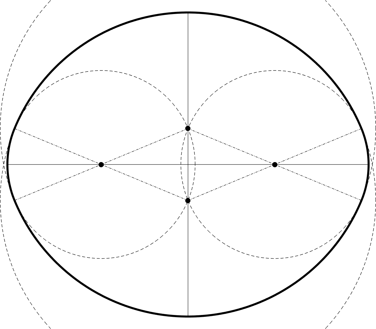
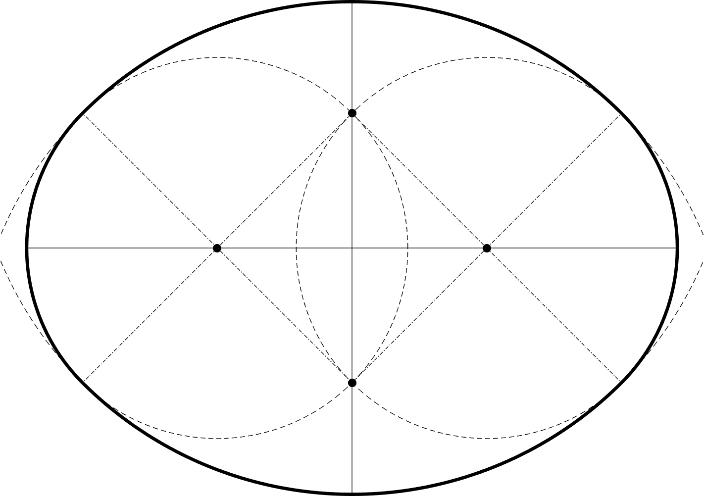
Figure 1: Left: Pseudo-ellipse $E_{\pi/4,1,2}$. Right: Squared pseudo-ellipse $E_{\pi/2,1,2}$. Pseudo-ellipses are represented with thick lines, their pairs of symmetry lines with thin continuous lines, their centers $O_{j}$ with solid dots, the circumferences of radii $r_{j}$ centered at $O_{j}$ with dashed thin lines, their angular ranges $[a_{j},b_{j}]$ with dash-dotted thin lines, and their nodes are the intersections of the thick and dash-dotted thin lines.

Pseudo-ellipses are the simplest examples. We may define them as the circular $4$-gons with a $\mathbb{Z}_{2}\times\mathbb{Z}_{2}$-symmetry. They form, modulo translations and rotations, a three-parameter family. The radii and central angles of any pseudo ellipse have the form

$$r_{1}=r_{3}=r,\qquad r_{2}=r_{4}=R,\qquad\delta_{1}=\delta_{3}=\alpha,\qquad\delta_{2}=\delta_{4}=\pi-\alpha,$$

for some free parameters $\alpha\in(0,\pi)$, and $r,R>0$. We will assume that $0<r<R$ for convenience. We will denote by $E_{\alpha,r,R}$ the corresponding pseudo-ellipse. Given any pseudo-ellipse $E_{\alpha,r,R}$, its centers form a rhombus (4 equal sides) and its nodes form a rectangle (4 equal angles). If $\alpha=\pi/2$, then $\delta_{1}=\delta_{2}=\delta_{3}=\delta_{4}=\pi/2$ and we say that $E_{\pi/2,r,R}$ is a squared pseudo-ellipse. The term squared comes from the fact that the centers of such pseudo-ellipses form a square. See Figure 1. The nodes of a squared pseudo-ellipse still form a rectangle, not a square. On the contrary, the celebrated Benettin-Strelcyn ovals, whose billiard dynamics was numerically studied in [6, 35, 44], are pseudo-ellipses whose nodes form a square, but whose centers only form a rhombus. Later on, the extend of chaos in billiards associated to general pseudo-ellipses was numerically studied in [24].

Another celebrated example of circular $4$-gon is Moss’s egg [22, Section 1.1], whose radii and central angles have the form

$$r_{1}=r,\quad r_{2}=2r=r_{4},\quad r_{3}=(2-\sqrt{2})r,\quad\delta_{1}=\pi,\quad\delta_{2}=\pi/4=\delta_{4},\quad\delta_{3}=\pi/2,$$

for some free parameter $r>0$, called the radius of the egg. All Moss’s eggs are congruent modulo similarities. They have a $\mathbb{Z}_{2}$-symmetry, so their nodes form an isosceles trapezoid (2 pairs of consecutive equal angles) and its centers form a kite (2 pairs of adjacent equal-length sides). In fact, this kite is a bit degenerate, since it looks like a triangle. See Figure 2. Billiards in a 2-parameter family of circular $4$-gons with $\mathbb{Z}_{2}$-symmetry, but not containing Moss’s egg, were considered in [4]. The heuristic analysis of sliding trajectories contained in Section 4.5 of that paper is closely related to our study.

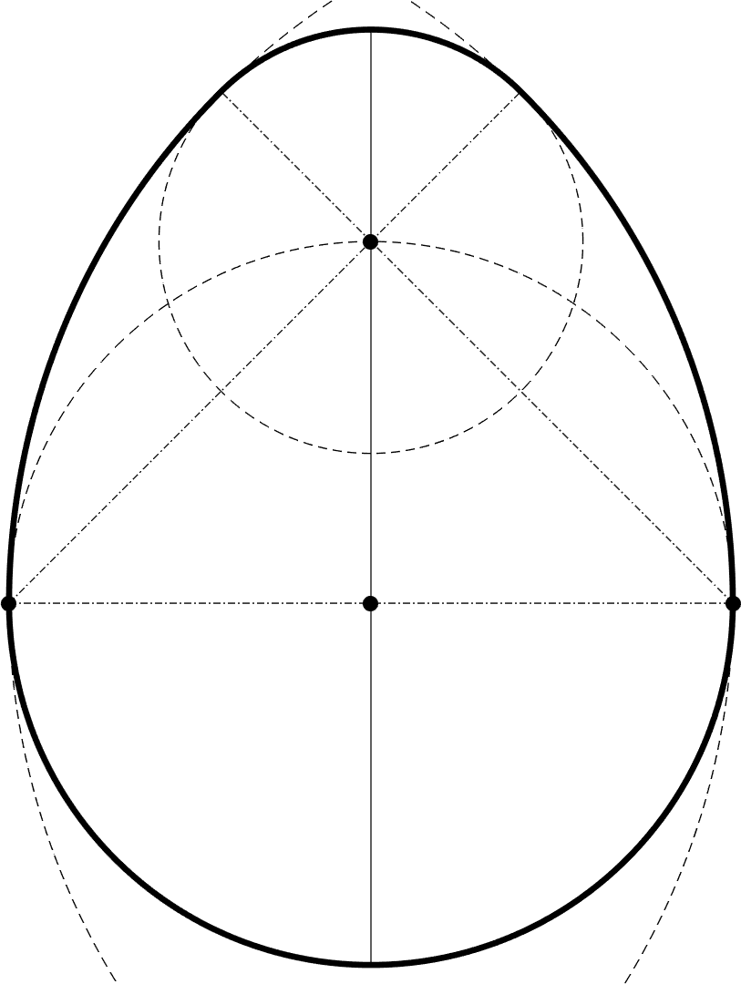
Figure 2: Left: Moss’s egg. Right: A nonsymmetric circular $6$-gon with centers $O_{1}=O_{4}=(3,-1)$, $O_{2}=O_{5}=(-1,-1)$ and $O_{3}=O_{6}=(0,1)$, which form a triangle. Circular polygons are represented with thick lines, the symmetry line of Moss’s egg with a thin continuous line, their centers $O_{j}$ with solid dots, the circumferences of radii $r_{j}$ centered at $O_{j}$ with dashed thin lines, their angular ranges $[a_{j},b_{j}]$ with dash-dotted thin lines, and their nodes are the intersections of the thick and dash-dotted thin lines.

Next, we describe a way to construct some circular $6$-gons. Fix a triangle $\triangle ABC$ with vertexes $A$, $B$ and $C$ ordered in the clockwise direction. Let $\alpha$, $\beta$ and $\gamma$ be its internal angles. Let $a$, $b$ and $c$ be the lengths of its sides, following the standard convention. That is, $a$ refers to the side opposed to vertex $A$ and so forth. Then we look for circular $6$-gons with centers $O_{1}=O_{4}=A$, $O_{2}=O_{5}=B$, $O_{3}=O_{6}=C$ and central angles $\delta_{1}=\delta_{4}=\alpha$, $\delta_{2}=\delta_{5}=\beta$ and $\delta_{3}=\delta_{6}=\gamma$. In this setting, all radii are determined by the choice of the first one. Namely, we can take

$$r_{1}=r,\quad r_{2}=r+c,\quad r_{3}=r+c-a,\quad r_{4}=r+c-a+b,\quad r_{5}=r+b-a,\quad r_{6}=r+b,$$

for any $r>\max\{0,a-c,a-b\}$. Therefore, we obtain a one-parameter family of parallel circular $6$-gons, parameterized by the first radius $r_{1}=r$. See Figure 2 for a non-symmetric sample with $A=(3,-1)$, $B=(-1,-1)$, $C=(0,1)$ and $r=1$.

One can draw circular polygons with many arcs by applying similar constructions, but that challenge is beyond the scope of this paper. The interested reader can look for inspiration in the nice Bunimovich’s construction of elliptic flowers [13].

To end this section, we emphasize that all our theorems are general. They can be applied to any circular polygon. Thus, we do not need to deal with concrete circular polygons.

3 The “stretching along the paths” method

In this section, we present the main ideas of the stretching along the paths method developed by Papini and Zanolin [49, 50], and extended by Pireddu and Zanolin [53, 54, 52]. It is a technical tool to establish the existence of topological chaos; that is, chaotic dynamics in continuous maps. We present a simplified version of the method because we work in the two-dimensional annulus $\mathcal{M}=\mathbb{T}\times[0,\pi]$ and our maps are homeomorphisms on $\mathcal{M}$. We also change some terminology because our maps stretch along vertical paths, instead of horizontal paths. The reader interested in more general statements about higher dimensions, finding fixed and periodic points in smaller compact sets, study of crossing numbers, non-invertible maps, and maps not defined in the whole space $\mathcal{M}$, is referred to the original references.

Let $\mathcal{M}=\mathbb{T}\times[0,\pi]$. By a continuum we mean a compact connected subset of $\mathcal{M}$. Paths and arcs are the continuous and the homeomorphic images of the unit interval $[0,1]$, respectively. Most definitions below are expressed in terms of paths, but we could also use arcs or continua, see [49, Table 3.1]. Cells are the homeomorphic image of the unit square $[0,1]^{2}$ so they are simply connected and compact. The Jordan-Shoenflies theorem implies that any simply connected compact subset of $\mathcal{M}$ bounded by a Jordan curve is a cell.

Definition 5.

An oriented cell $\widetilde{\mathcal{Q}}$ is a cell $\mathcal{Q}\subset\mathcal{M}$ where we have chosen four different points $\widetilde{\mathcal{Q}}_{\rm bl}$ (base-left), $\widetilde{\mathcal{Q}}_{\rm br}$ (base-right), $\widetilde{\mathcal{Q}}_{\rm tr}$ (top-right) and $\widetilde{\mathcal{Q}}_{\rm tl}$ (top-left) over the boundary $\partial\mathcal{Q}$ in a counter-clockwise order. The base side of $\widetilde{\mathcal{Q}}$ is the arc $\widetilde{\mathcal{Q}}_{\rm b}\subset\partial\mathcal{Q}$ that goes from $\widetilde{\mathcal{Q}}_{\rm bl}$ to $\widetilde{\mathcal{Q}}_{\rm br}$ in the counter-clockwise orientation. Similarly, $\widetilde{\mathcal{Q}}_{\rm l}$, $\widetilde{\mathcal{Q}}_{\rm r}$ and $\widetilde{\mathcal{Q}}_{\rm t}$ are the left, right and top sides of $\widetilde{\mathcal{Q}}$. Finally, $\widetilde{\mathcal{Q}}_{\rm h}=\widetilde{\mathcal{Q}}_{\rm b}\cup\widetilde{\mathcal{Q}}_{\rm t}$ and $\widetilde{\mathcal{Q}}_{\rm v}=\widetilde{\mathcal{Q}}_{\rm l}\cup\widetilde{\mathcal{Q}}_{\rm r}$ are the horizontal and vertical sides of $\widetilde{\mathcal{Q}}$.

All our cells will have line segments as vertical sides, some being even quadrilaterals.

Definition 6.

Let $\widetilde{\mathcal{Q}}$ be an oriented cell. A path $\gamma:[a,b]\to Q$ is vertical (respectively, horizontal) in $\widetilde{\mathcal{Q}}$ when it connects the two horizontal (respectively, vertical) sides of $\widetilde{\mathcal{Q}}$ and $\gamma(t)\not\in\widetilde{\mathcal{Q}}_{\rm h}$ (respectively, $\gamma(t)\not\in\widetilde{\mathcal{Q}}_{\rm v}$) for all $t\in(a,b)$. We say that an oriented cell $\widetilde{\mathcal{K}}$ is a horizontal slab in $\widetilde{\mathcal{Q}}$ and write

$$\widetilde{\mathcal{K}}\subset_{\rm h}\widetilde{\mathcal{Q}}$$

when $\mathcal{K}\subset\mathcal{Q}$ and, either $\widetilde{\mathcal{K}}_{\rm l}\subset\widetilde{\mathcal{Q}}_{\rm l}$ and $\widetilde{\mathcal{K}}_{\rm r}\subset\widetilde{\mathcal{Q}}_{\rm r}$, or $\widetilde{\mathcal{K}}_{\rm l}\subset\widetilde{\mathcal{Q}}_{\rm r}$ and $\widetilde{\mathcal{K}}_{\rm r}\subset\widetilde{\mathcal{Q}}_{\rm l}$. If, in addition, $\mathcal{K}\cap\widetilde{\mathcal{Q}}_{\rm h}=\emptyset$, then we say that $\tilde{\mathcal{K}}$ is a strict horizontal slab in $\widetilde{\mathcal{Q}}$ and write

$$\widetilde{\mathcal{K}}\varsubsetneq_{\rm h}\widetilde{\mathcal{Q}}.$$

Vertical slabs can be analogously defined. Note that $\widetilde{\mathcal{K}}\varsubsetneq_{\rm h}\widetilde{\mathcal{Q}}$ is a much stronger condition than $\widetilde{\mathcal{K}}\subset_{\rm h}\widetilde{\mathcal{Q}}$ and $\mathcal{K}\varsubsetneq\mathcal{Q}$.

Definition 7.

Let $g:\mathcal{M}\to\mathcal{M}$ be a homeomorphism. Let $\widetilde{\mathcal{Q}}$ and $\widetilde{\mathcal{Q}}^{\prime}$ be oriented cells in $\mathcal{M}$. We say that $g$ stretches $\widetilde{\mathcal{Q}}$ to $\widetilde{\mathcal{Q}}^{\prime}$ along vertical paths and write

$$g:\widetilde{\mathcal{Q}}\rightsquigarrow\widetilde{\mathcal{Q}}^{\prime}$$

when every path $\gamma:[a,b]\to\mathcal{Q}$ that is vertical in $\widetilde{\mathcal{Q}}$ contains a subpath $\gamma^{\prime}=\gamma_{|[s,t]}$ for some $a\leq s<t\leq b$ such that the image path $g\circ\gamma^{\prime}:[s,t]\to\mathcal{Q}^{\prime}$ is vertical in $\widetilde{\mathcal{Q}}^{\prime}$.

This stretching condition does not imply that $g(\mathcal{Q})\subset\mathcal{Q}^{\prime}$. In fact, we see $\mathcal{Q}^{\prime}$ as a ‘target set’ that we want to ‘visit’, and not as a codomain. If $\gamma:[a,b]\to\mathcal{M}$ is a path, we also use the notation $\gamma$ to mean the set $\gamma([a,b])\subset\mathcal{M}$. This allows us to estate the stretching condition more succinctly. Namely, we ask that every path $\gamma$ vertical in $\widetilde{\mathcal{Q}}$ contains a subpath $\gamma^{\prime}\subset\gamma$ such that the image path $g(\gamma^{\prime})$ is vertical in $\widetilde{\mathcal{Q}}^{\prime}$.

Definition 8.

Let $f:\mathcal{M}\to\mathcal{M}$ be a homeomorphism. Let $(\mathcal{Q}_{i};n_{i})_{i\in I}$ be a two-sided sequence: $I\in\mathbb{Z}$, one-sided sequence: $I\in\mathbb{N}_{0}=\mathbb{N}\cup\{0\}$, $p$-periodic sequence: $I=\mathbb{Z}/p\mathbb{Z}$, or finite sequence $I=\{0,1,\ldots,k\}$ with $\mathcal{Q}_{i}\subset\mathcal{M}$ and $n_{i}\in\mathbb{N}$. Let $x\in\mathcal{Q}_{0}$. We say that the point $x$ $f$-realizes the sequence $(\mathcal{Q}_{i};n_{i})_{i\in I}$ when

$$f^{-(n_{-1}+\cdots+n_{-i})}(x)\in\mathcal{Q}_{-i},\qquad f^{n_{0}+\cdots+n_{i-1}}(x)\in\mathcal{Q}_{i},\qquad\forall i\geq 1.$$

Clearly, condition $f^{-(n_{-1}+\cdots+n_{-i})}(x)\in\mathcal{Q}_{-i}$ does not apply in the case of one-sided or finite sequences. A subset of $\mathcal{Q}_{0}$ $f$-realizes the sequence $(\mathcal{Q}_{i};n_{i})_{i\in I}$ when all its points do so.

The subsets $\mathcal{Q}_{i}$ in this definition do not have to be cells, but that is the case considered in the following powerful 3-in-1 theorem about the existence of points and paths of the phase space $\mathcal{M}$ that $f$-realize certain two-sided, one-sided, and periodic sequences of oriented cells.

Theorem 9 (Papini & Zanolin [50]).

Let $f:\mathcal{M}\to\mathcal{M}$ be a homeomorphism. Let $(\widetilde{\mathcal{Q}}_{i};n_{i})_{i\in I}$ be a two-sided, one-sided or $p$-periodic sequence where $\widetilde{\mathcal{Q}}_{i}$ are oriented cells with $\mathcal{Q}_{i}\subset\mathcal{M}$ and $n_{i}\in\mathbb{N}$. If

$$f^{n_{i}}:\widetilde{\mathcal{Q}}_{i}\rightsquigarrow\widetilde{\mathcal{Q}}_{i+1},\qquad\forall i,$$

then the following versions hold.

• If $I=\mathbb{Z}$, there is a point $x\in\mathcal{Q}_{0}$ that $f$-realizes the two-sided sequence $(\mathcal{Q}_{i};n_{i})_{i\in\mathbb{Z}}$.

• If $I=\mathbb{N}_{0}$, there is a path $\gamma$ horizontal in $\widetilde{\mathcal{Q}}_{0}$ that $f$-realizes the sequence $(\mathcal{Q}_{i};n_{i})_{i\geq 0}$.

• If $(\widetilde{\mathcal{Q}}_{i+p};n_{i+p})=(\widetilde{\mathcal{Q}}_{i};n_{i})$ for all $i\in\mathbb{Z}$ and $n=n_{0}+\cdots+n_{p-1}$, there is a point $x\in\mathcal{Q}_{0}$ such that $f^{n}(x)=x$ and $x$ $f$-realizes the $p$-periodic sequence $(\mathcal{Q}_{i};n_{i})_{i\in\mathbb{Z}/p\mathbb{Z}}$.

Remark 10.

We believe that the following finite version (F) also holds: “If $I=\{0,\ldots,k\}$, there is a horizontal slab $\widetilde{\mathcal{K}}\subset_{\rm h}\widetilde{\mathcal{Q}}_{0}$ such that $\mathcal{K}$ $f$-realizes the finite sequence $(\mathcal{Q}_{i};n_{i})_{i=0,\ldots,k}$.”, but we have not found such statement in the literature. Therefore, we will not use it.

We refer to Theorem 2.2 in [50] for a more general statement which deals with sequences of maps that are not some power iterates of a single map. Version (T) of Theorem 9 is the key tool to obtain orbits that follow prescribed itineraries, so that we can establish the existence of topological chaos and we can construct a suitable symbolic dynamics in Section 6. We will use version (O) of Theorem 9 to prove the existence of ‘paths’ of generic sliding billiard trajectories that approach the boundary asymptotically with optimal uniform speed in Section 7. Finally, we will establish several lower bounds on the number of periodic billiard trajectories from version (P) of Theorem 9 in Section 8.

4 The fundamental lemma for circular polygons

To begin with, we list some notations used along this section. Let $\Gamma$ be a circular $k$-gon with arcs $\Gamma_{j}$, centers $O_{j}$, radii $r_{j}$, singularities $a_{j}$, and central angles $\delta_{j}$. Set $b_{j}=a_{j+1}$ and $\mu_{j}=\sqrt{r_{j}/r_{j+1}}$. Recall that index $j$ is defined modulo $k$. Let $z:\mathbb{T}\to\Gamma$ be the polar parametrisation of $\Gamma$ introduced in Definition 3.

Let $\mathcal{M}=\mathbb{T}\times[0,\pi]$, and let $(\varphi,\theta)\in\mathrm{Int}\,\mathcal{M}$. Write $z=z(\varphi)$ and $v=R_{\theta}z^{\prime}(\varphi)$ where $R_{\theta}$ is the standard $2\times 2$ counter-clockwise rotation matrix by an angle $\theta$. The straight line $L=L(\varphi,\theta)$ passing through $z$ in the direction $v$ has exactly two points of intersection with $\Gamma$ since $\theta\in(0,\pi)$. One of these is $z$; denote by $\bar{z}$ the other. Then there is a unique $\bar{\varphi}\in\mathbb{T}$ such that $\bar{z}=z(\bar{\varphi})$. Denote by $\bar{\theta}$ the angle between $L$ and $z^{\prime}(\bar{\varphi})$ in the counter-clockwise direction. The billiard map $f:\mathrm{Int}\,\mathcal{M}\to\mathrm{Int}\,\mathcal{M}$ is defined by $f(\varphi,\theta)=(\bar{\varphi},\bar{\theta})$, see Figure 3.

Figure 3: Definition of the billiard map $f(\varphi,\theta)=(\bar{\varphi},\bar{\theta})$.

Note that $f$ is continuous since $\Gamma$ is $C^{1}$ and strictly convex. The billiard map can be extended continuously to $\partial\mathcal{M}$ by setting $f(\varphi,0)=(\varphi,0)$ and $f(\varphi,\pi)=(\varphi,\pi)$ for each $\varphi\in\mathbb{T}$. The billiard map $f:\mathcal{M}\to\mathcal{M}$ is a homeomorphism; indeed, the map $f^{-1}=I\circ f\circ I$ is a continuous inverse where the involution $I:\mathcal{M}\to\mathcal{M}$ is defined by $I(\varphi,\theta)=(\varphi,\pi-\theta)$.

A key geometric property of the billiard dynamics in the case of impacts in consecutive arcs was presented in [36]. Later on, a more detailed description was given in [4]. Both results follow from trigonometric arguments. Recall that $\delta_{j}=b_{j}-a_{j}$ and $b_{j}=a_{j+1}$.

Lemma 11.

The billiard map $f:\mathcal{M}\to\mathcal{M}$ satisfies the following properties.

1. If $a_{j}\leq\varphi\leq\varphi+2\theta\leq b_{j}$, then $(\bar{\varphi},\bar{\theta})=f(\varphi,\theta)=(\varphi+2\theta,\theta)$.

2. Let $g(\theta;\mu)=\mskip 2.0mu{\rm acos}\mskip 1.0mu\big{(}(1-\mu^{2})+\mu^{2}\cos\theta\big{)}$. If $0<\theta\leq\delta_{j}$ and $\bar{\theta}=g(\theta;\mu_{j})\leq\delta_{j+1}$, then

   $$f(b_{j}-\theta,\theta)=(a_{j+1}+\bar{\theta},\bar{\theta})\qquad\mbox{and}\qquad\begin{cases}\bar{\theta}<\mu_{j}\theta,&\mbox{when $\mu_{j}<1$,}\\ \bar{\theta}>\mu_{j}\theta,&\mbox{when $\mu_{j}>1$.}\end{cases}$$ (5)

3. Given any $\epsilon>0$ there exists $\psi=\psi(\epsilon)>0$ such that

   $$\left.\begin{array}[]{c}f(\varphi,\theta)=(\bar{\varphi},\bar{\theta})\mbox{ with }0<\theta\leq\psi\\ \mbox{and }a_{j}\leq\varphi\leq a_{j+1}\leq\bar{\varphi}\leq a_{j+2}\\ \end{array}\right\}\Rightarrow\begin{cases}\bar{\theta}>(\mu_{j}-\epsilon)\theta,&\mbox{when $\mu_{j}<1$,}\\ \bar{\theta}<(\mu_{j}+\epsilon)\theta,&\mbox{when $\mu_{j}>1$.}\end{cases}$$

Proof.

1. If $a_{j}\leq\varphi\leq\varphi+2\theta\leq b_{j}$, then $z(\varphi),z(\varphi+2\theta)\in\Gamma_{j}$, so $f$ behaves as a circular billiard map, in which case is well-known that $f(\varphi,\theta)=(\varphi+2\theta,\theta)$.

2. Set $\varphi=b_{j}-\theta$ and $(\bar{\varphi},\bar{\theta})=f(\varphi,\theta)$. Condition $0<\theta\leq\delta_{j}$ implies that $z(\varphi)\in\Gamma_{j}$. Identity $\varphi+\theta=b_{j}$ implies that lines $L=L(\varphi,\theta)$ and $N_{j}$ are perpendicular, where $N_{j}$ is the normal to $\Gamma$ at $z(b_{j})$. If, in addition, $z(\bar{\varphi})\in\Gamma_{j+1}$, then Hubacher proved (5) in [36, page 486]. Finally, we note that $\bar{\theta}\leq\delta_{j+1}$ implies that $z(\bar{\varphi})\in\Gamma_{j+1}$.

3. Bálint et al. [4] proved the following generalization of Hubacher computation. Set $f(\varphi,\theta)=(\bar{\varphi},\bar{\theta})$. If $a_{j}\leq\varphi\leq a_{j+1}\leq\bar{\varphi}\leq a_{j+2}$, so that $z(\varphi)\in\Gamma_{j}$ and $z(\bar{\varphi})\in\Gamma_{j+1}$, then there exist angles $\varphi^{+}\in[0,2\theta]$ and $\varphi^{-}\in[0,2\bar{\theta}]$ such that

   $$\varphi=b_{j}-\varphi^{+},\qquad\bar{\varphi}=a_{j+1}+\varphi^{-},\qquad\varphi^{+}+\varphi^{-}=\theta+\bar{\theta},$$

   and

   $$\bar{\theta}=\mskip 2.0mu{\rm acos}\mskip 1.0mu\left((1-\mu^{2}_{j})\cos(\theta-\varphi^{+})+\mu^{2}_{j}\cos\theta\right).$$

   Hubacher computation corresponds to the case $\varphi^{+}=\theta$ and $\varphi^{-}=\bar{\theta}$.

   A straightforward computation with Taylor expansions shows that

   $$\bar{\theta}=\Omega_{j}(s)\theta+\mathop{\rm O}\nolimits(\theta^{3}),\quad\Omega_{j}(s)=\sqrt{\mu_{j}^{2}+(1-\mu_{j}^{2})s^{2}},\quad s=1-\varphi^{+}/\theta\in[-1,1],$$ (6)

   as $\theta\to 0^{+}$. Function $\Omega_{j}(s)$ is even and $\Omega_{j}(0)=\mu_{j}$. Besides, $\Omega_{j}^{2}(s)=\mu_{j}^{2}+(1-\mu_{j}^{2})s^{2}$. If $\mu_{j}<1$, then $\Omega_{j}(s)$ increases for $s>0$ and decreases for $s<0$, so $\Omega_{j}(s)\geq\mu_{j}$ for all $s\in[-1,1]$. If $\mu_{j}>1$, then $\Omega_{j}(s)$ decreases for $s>0$ and increases for $s<0$, so $\Omega_{j}(s)\leq\mu_{j}$ for all $s\in[-1,1]$. ∎

If $a_{j}\leq\varphi<\varphi+2\theta=b_{j}$, then $z(\varphi)\in\Gamma_{j}$ and $z(\bar{\varphi})=b_{j}=a_{j+1}\in\Gamma_{j}\cap\Gamma_{j+1}$, but part (a) of Lemma 11 still applies, because the tangents to $\Gamma_{j}$ and $\Gamma_{j+1}$ agree at $z(\bar{\varphi})$ by the definition of circular polygon. This fact will be used in Proposition 50 to construct some special periodic nodal billiard trajectories in rational circular polygons, which are introduced in Definition 49. Similar nodal periodic billiard trajectories were constructed in [10] to answer a question about length spectrum and rigidity.

Lemma 11 and the above observation describe two rather different ways in which the angle $\theta$ can vary as a sliding billiard trajectory jumps from one arc to the next. On the one hand, if the trajectory impacts at the corresponding node, there is no change: $\bar{\theta}=\theta$. On the other hand, if the billiard trajectory is perpendicular at the normal line at the corresponding node, we have the largest possible change: $\bar{\theta}<\mu_{j}\theta$ for $\mu_{j}<1$ or $\bar{\theta}>\mu_{j}\theta$ for $\mu_{j}>1$. The great contrast between these two situations is the crucial fact behind the non-existence of caustics near the boundary obtained by Hubacher [36]. It is also the main ingredient to obtain all chaotic properties stated in the introduction.

Next, we introduce the main geometric subsets of the phase space $\mathcal{M}=\mathbb{T}\times[0,\pi]$. All of them are denoted with calligraphic letters.

Definition 12.

The $j$-singularity segment is the vertical segment $\mathcal{L}_{j}=\{a_{j}\}\times[0,\pi]\subset\mathcal{M}$. Given any $s>0$, the $(j,\pm s)$-singularity segment are the slanted segments

$$\mathcal{L}_{j}^{-s}=\big{\{}(\varphi,\theta)\in\mathcal{M}:a_{j-1}\leq\varphi=a_{j}-2\theta s\big{\}},\quad\mathcal{L}_{j}^{s}=\big{\{}(\varphi,\theta)\in\mathcal{M}:\varphi=a_{j}+2\theta s\leq a_{j+1}\big{\}}.$$

The $j$-fundamental domain is the triangular domain

$$\mathcal{D}_{j}=\left\{(\varphi,\theta)\in\mathcal{M}:a_{j}\leq\varphi\leq a_{j}+2\theta\leq a_{j+1}\right\}.$$

Finally, $\mathcal{L}=\bigcup_{j=1}^{k}\left(\mathcal{L}_{j}\cup\mathcal{L}_{j}^{1/2}\cap\mathcal{L}_{j}^{1}\right)$ is the extended singularity set.

Note that $\mathcal{L}^{n}_{j}\subset f^{n}(\mathcal{L}_{j})$ for all $n\in\mathbb{Z}$, so $\mathcal{L}^{s}_{j}$ is a generalization of the forward and backward iterates under the billiard map of the $j$-singularity segments when $s\not\in\mathbb{Z}$. We will only need the segments $\mathcal{L}^{s}_{j}$ for values $s=n$ and $s=n+1/2$ with $n\in\mathbb{Z}$. The left (respectively, right) side of the triangle $\mathcal{D}_{j}$ is contained in the vertical segment $\mathcal{L}_{j}$ (respectively, coincides with the slanted segment $\mathcal{L}_{j}^{1}$).

We have used the term ‘sliding’ in a clumsy way until now. Let us clarify its precise meaning. Let $\Pi_{\varphi}:\mathcal{M}\to\mathbb{T}$ and $\Pi_{\theta}:\mathcal{M}\to[0,\pi]$ be the projections $\Pi_{\varphi}(\varphi,\theta)=\varphi$ and $\Pi_{\theta}(\varphi,\theta)=\theta$. Let $J:\mathcal{M}\setminus\mathcal{L}\to\mathbb{Z}/k\mathbb{Z}$ be the piece-wise constant map defined by $a_{j}<\Pi_{\varphi}(x)<b_{j}\Rightarrow J(x)=j$. This map is well-defined since $\Pi_{\varphi}(x)\not\in\{a_{1},\ldots,a_{k}\}=\{b_{1},\ldots,b_{k}\}$ when $x\not\in\mathcal{L}$.

Definition 13.

A billiard orbit is (counter-clockwise) sliding when any consecutive impact points are either in the same arc or in consecutive arcs in the counter-clockwise direction. An orbit is generic when it avoids the extended singularity set. We denote by $\mathcal{S}_{0}$ the set of all initial conditions that give rise to generic counter-clockwise sliding orbits. That is,

$$\mathcal{S}_{0}=\left\{x\in\mathcal{M}:\mbox{$J(f^{n+1}(x))-J(f^{n}(x))\in\{0,1\}$ and $f^{n}(x)\not\in\mathcal{L}$ for all $n\in\mathbb{Z}$}\right\}.$$

The (counter-clockwise) generic sliding set $\mathcal{S}_{0}$ is $f$-invariant. The term glancing —see, for instance,  [46]— is also used in the literature, but sliding is the most widespread term. A consequence of part (a) of Lemma 11 is that any generic sliding billiard orbit has exactly one point in $\mathop{\rm Int}\nolimits\mathcal{D}_{j}$ on each turn around $\Gamma$. This fact establishes the fundamental character of $\mathcal{D}_{j}$. Following the notation used in the introduction, $\mathcal{S}_{\pi}$ is the clockwise generic sliding set, but we are not going to deal with it.

Remark 14.

If $x\in\mathcal{M}$ is a point such that $x_{i}=(\varphi_{i},\theta_{i})=f^{i}(x)\in\mathcal{L}$ for some $i\in\mathbb{Z}$, then its billiard trajectory $\big{(}z_{n}=z(\Pi_{\varphi}(f^{n}(x)))\big{)}_{n\in\mathbb{Z}}$ has some impact point $z_{m}\in\Gamma_{\star}$, where $\Gamma_{\star}$ is the set of nodes (1), or has two consecutive impact points $z_{m}\in\Gamma_{j}$ and $z_{m+1}\in\Gamma_{j+1}$ such that the segment from $z_{m}$ to $z_{m+1}$ is perpendicular to the normal to $\Gamma$ at the node $\Gamma_{j}\cap\Gamma_{j+1}$.

Lemma 15.

Let $s,t\geq 0$ and $j\mod k$ such that $s+t\geq\delta_{j}/2\pi$. Then $\mathcal{L}_{j}^{s}\cap\mathcal{L}_{j+1}^{-t}\neq\emptyset$ and

$$\Pi_{\varphi}\left(\mathcal{L}_{j}^{s}\cap\mathcal{L}_{j+1}^{-t}\right)=a_{j}+\frac{s\delta_{j}}{s+t},\qquad\Pi_{\theta}\left(\mathcal{L}_{j}^{s}\cap\mathcal{L}_{j+1}^{-t}\right)=\frac{\delta_{j}}{2s+2t}.$$

Proof.

By definition, $(\varphi,\theta)\in\mathcal{L}_{j}^{s}\cap\mathcal{L}_{j+1}^{-t}\Leftrightarrow a_{j}\leq a_{j}+2\theta s=\varphi=a_{j+1}-2\theta t\leq a_{j+1}$. Identity $a_{j}+2\theta s=a_{j+1}-2\theta t$ implies that $2\theta=\delta_{j}/(s+t)$. Then inequality $s+t\geq\delta_{j}/2\pi$ implies that $\theta\leq\pi$. Finally, $a_{j}+2\theta s\leq a_{j+1}$ and $a_{j+1}-2\theta t\geq a_{j}$ because $s/(s+t),t/(s+t)\leq 1$. ∎

This lemma implies that segments $\mathcal{L}_{j+1}^{-n+1}$ and $\mathcal{L}_{j+1}^{-n}$ intersect segments $\mathcal{L}_{j}$ and $\mathcal{L}_{j}^{1}$ for any integer $n\geq 2>1+\delta_{j}/2\pi$, so the following definition makes sense. See Figure 4.

Definition 16.

Let $n$ be an integer such that $n\geq 2$. The $(j,n)$-fundamental quadrilateral is the oriented cell $\widetilde{\mathcal{Q}}_{j,n}\subset\mathcal{M}$ bounded by $\mathcal{L}_{j}$ (left side), $\mathcal{L}_{j+1}^{-n}$ (base side), $\mathcal{L}_{j}^{1}$ (right side) and $\mathcal{L}_{j+1}^{-n+1}$ (top side). We split $\mathcal{Q}_{j,n}$ in two by means of the segment $\mathcal{L}_{j}^{-n+1/2}$, which gives rise to two smaller oriented cells: $\widetilde{\mathcal{Q}}^{-}_{j,n}$ (the lower one) and $\widetilde{\mathcal{Q}}^{+}_{j,n}$ (the upper one), whose left and right sides are still contained in $\mathcal{L}_{j}$ and $\mathcal{L}_{j}^{1}$, respectively. We say that $\tilde{\mathcal{Q}}^{\pm}_{j,n}$ is the $(\pm,j,n)$-fundamental quadrilateral.

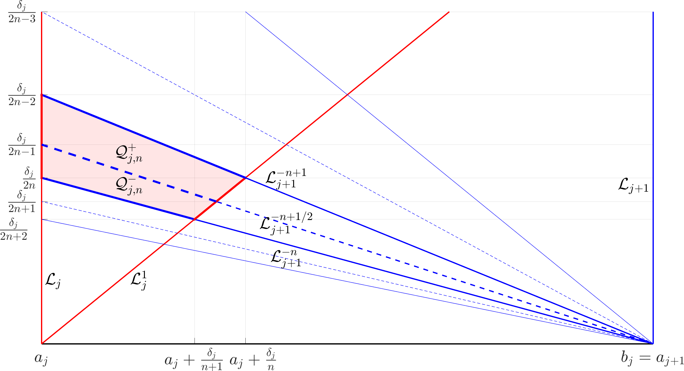
Figure 4: The fundamental quadrilateral $\mathcal{Q}_{j,n}=\mathcal{Q}^{-}_{j,n}\cup\mathcal{Q}^{+}_{j,n}$. Its horizontal (base and top) and vertical (left and right) sides are displayed in blue and red, respectively. Accordingly, singularity segments $\mathcal{L}^{s}_{j}$ and $\mathcal{L}^{-t}_{j+1}$ are displayed in red and blue, respectively. Besides, they are displayed with continuous and dashed lines when $s,t\in\mathbb{N}$ and $t\in\mathbb{N}+\frac{1}{2}$, respectively. This is a quantitative representation computed for $\delta_{j}=\pi/2$ and $n=3$. The images $f^{n}(\mathcal{Q}^{\pm}_{j,n})$ are displayed in Figure 5.

In order to find sufficient conditions for $f^{n}:\widetilde{\mathcal{Q}}^{\varsigma}_{j,n}\rightsquigarrow\widetilde{\mathcal{Q}}^{\varsigma^{\prime}}_{j+1,n^{\prime}}$, we need the extreme values of $\Pi_{\theta}(f^{n}(x))$ when $x$ moves on the horizontal sides of $\widetilde{\mathcal{Q}}^{\varsigma}_{j,n}$ and the extreme values of $\Pi_{\theta}(x)$ when $x\in\mathcal{Q}_{j+1,n^{\prime}}=\mathcal{Q}^{-}_{j+1,n^{\prime}}\cup\mathcal{Q}^{+}_{j+1,n^{\prime}}$. These extreme values are estimated below.

Lemma 17.

Fix any $j\mod k$. With the above notations, if $\chi_{j}\geq 2$ is a large enough integer, then the following properties hold for all $n\geq\chi_{j}$.

1. $\nu_{j,n}:=\min_{x\in\mathcal{Q}_{j,n}}\Pi_{\theta}(x)=\delta_{j}/(2n+2)$ and $\omega_{j,n}:=\max_{x\in\mathcal{Q}_{j,n}}\Pi_{\theta}(x)=\delta_{j}/(2n-2)$.

2. If $\nu^{s}_{j,n}:=\min_{x\in\mathcal{Q}_{j,n}\cap\mathcal{L}^{-n+s}_{j+1}}\Pi_{\theta}(f^{n}(x))$ and $\omega^{s}_{j,n}:=\max_{x\in\mathcal{Q}_{j,n}\cap\mathcal{L}^{-n+s}_{j+1}}\Pi_{\theta}(f^{n}(x))$, then

   1. $\nu^{0}_{j,n}=\delta_{j}/(2n+2)$, $\nu^{1}_{j,n}=\delta_{j}/2n=\omega^{0}_{j,n}$ and $\omega^{1}_{j,n}=\delta_{j}/(2n-2)$;

   2. $\omega^{1/2}_{j,n}<\mu_{j}\delta_{j}/(2n-1)$ when $\mu_{j}<1$; and

   3. $\nu^{1/2}_{j,n}>\mu_{j}\delta_{j}/(2n+1)$ when $\mu_{j}>1$.

Proof.

The fundamental domain $\mathcal{Q}_{j,n}$ is only well-defined for $n\geq 2$. The reader must keep in mind Lemmas 11 and 15. See Figure 4 for a visual guide.

1. The minimum and maximum values are attained at the intersections $\mathcal{L}_{j}^{1}\cap\mathcal{L}_{j+1}^{-n}$ and $\mathcal{L}_{j}\cap\mathcal{L}_{j+1}^{-n+1}$, respectively.

2. 1. If $x\in\mathcal{Q}_{j,n}\cap\mathcal{L}^{-n}_{j+1}$ or $x\in\mathcal{Q}_{j,n}\cap\mathcal{L}^{-n+1}_{j+1}$, then $\Pi_{\theta}(f^{n}(x))=\Pi_{\theta}(x)$ by part (a) of Lemma 11. Therefore, the four extreme values $\nu^{0}_{j,n}$, $\nu^{1}_{j,n}$, $\omega^{0}_{j,n}$ and $\omega^{1}_{j,n}$ are attained at the four intersections $\mathcal{L}_{j}^{1}\cap\mathcal{L}_{j+1}^{-n}$, $\mathcal{L}_{j}^{1}\cap\mathcal{L}_{j+1}^{-n+1}$, $\mathcal{L}_{j}\cap\mathcal{L}_{j+1}^{-n}$ and $\mathcal{L}_{j}\cap\mathcal{L}_{j+1}^{-n+1}$, respectively.

   2. First, the value $\max_{x\in\mathcal{Q}_{j,n}\cap\mathcal{L}^{-n+1/2}_{j+1}}\Pi_{\theta}(x)$ is attained at $\mathcal{L}_{j}\cap\mathcal{L}_{j+1}^{-n+1/2}$. Second, if $x\in\mathcal{Q}_{j,n}\cap\mathcal{L}^{-n+1/2}_{j+1}$ and $\mu_{j}<1$, then $\Pi_{\theta}(f^{n}(x))<\mu_{j}\Pi_{\theta}(x)$ by part (b) of Lemma 11.

      We need hypotheses $0<\theta\leq\delta_{j}$ and $\bar{\theta}=g(\theta;\mu_{j})\leq\delta_{j+1}$ to apply Lemma 11. In order to guarantee them, it suffices to take $n\geq\chi_{j}$ with

      $$\chi_{j}\geq 1+\lceil\mu_{j}\delta_{j}/2\delta_{j+1}\rceil,$$ (7)

      since then $\chi_{j}\geq 2$ and $2\chi_{j}-2\geq\mu_{j}\delta_{j}/\delta_{j+1}$, so $\theta\leq\omega_{j,n}\leq\delta_{j}/(2\chi_{j}-2)\leq\delta_{j}/2<\delta_{j}$ and $\bar{\theta}<\mu_{j}\theta\leq\mu_{j}\delta_{j}/(2\chi_{j}-2)\leq\delta_{j+1}$. Here $\lceil\cdot\rceil$ denotes the ceil function.

   3. First, the value $\min_{x\in\mathcal{Q}_{j,n}\cap\mathcal{L}^{-n+1/2}_{j+1}}\Pi_{\theta}(x)$ is attained at $\mathcal{L}_{j}^{1}\cap\mathcal{L}_{j+1}^{-n+1/2}$. Second, if $x\in\mathcal{Q}_{j,n}\cap\mathcal{L}^{-n+1/2}_{j+1}$ and $\mu_{j}>1$, then $\Pi_{\theta}(f^{n}(x))>\mu_{j}\Pi_{\theta}(x)$ by part (b) of Lemma 11. We still need hypotheses $0<\theta\leq\delta_{j}$ and $\bar{\theta}=g(\theta;\mu_{j})\leq\delta_{j+1}$ in Lemma 11. In order to guarantee them, it suffices to take $n\geq\chi_{j}$ for some large enough integer $\chi_{j}$, since $\lim_{n\to+\infty}\omega_{j,n}=0$ and $\lim_{\theta\to 0^{+}}g(\theta;\mu_{j})=0$. ∎

The following lemma (which we refer to as the fundamental lemma) is the key step in constructing generic sliding billiard trajectories that approach the boundary in optimal time, and in constructing symbolic dynamics. It describes which fundamental quadrilaterals in $\mathcal{D}_{j+1}$ we can ‘nicely’ visit if we start in a given fundamental quadrilateral in $\mathcal{D}_{j}$. See Figure 5 for a visual guide.

Lemma 18 (Fundamental Lemma).

With the above notations, let

$$\Upsilon_{j}=\left\{(n,n^{\prime})\in\mathbb{N}^{2}:\alpha_{j}^{-}n+\beta_{j}^{-}\leq n^{\prime}\leq\alpha_{j}^{+}n-\beta_{j}^{+},\ n\geq\chi_{j},\ n^{\prime}\geq\chi_{j+1}\right\},$$ (8)

where $\alpha_{j}^{-}=\delta_{j+1}/\delta_{j}\max\{1,\mu_{j}\}$, $\alpha_{j}^{+}=\delta_{j+1}/\delta_{j}\min\{1,\mu_{j}\}$ and $\beta_{j}^{\pm}=\alpha_{j}^{\pm}+1$ for all $j\mod k$. Then $f^{n}:\widetilde{\mathcal{Q}}^{\varsigma}_{j,n}\rightsquigarrow\widetilde{\mathcal{Q}}^{\varsigma^{\prime}}_{j+1,n^{\prime}}$ for all $j\mod k$, $(n,n^{\prime})\in\Upsilon_{j}$ and $\varsigma,\varsigma^{\prime}\in\{-,+\}$.

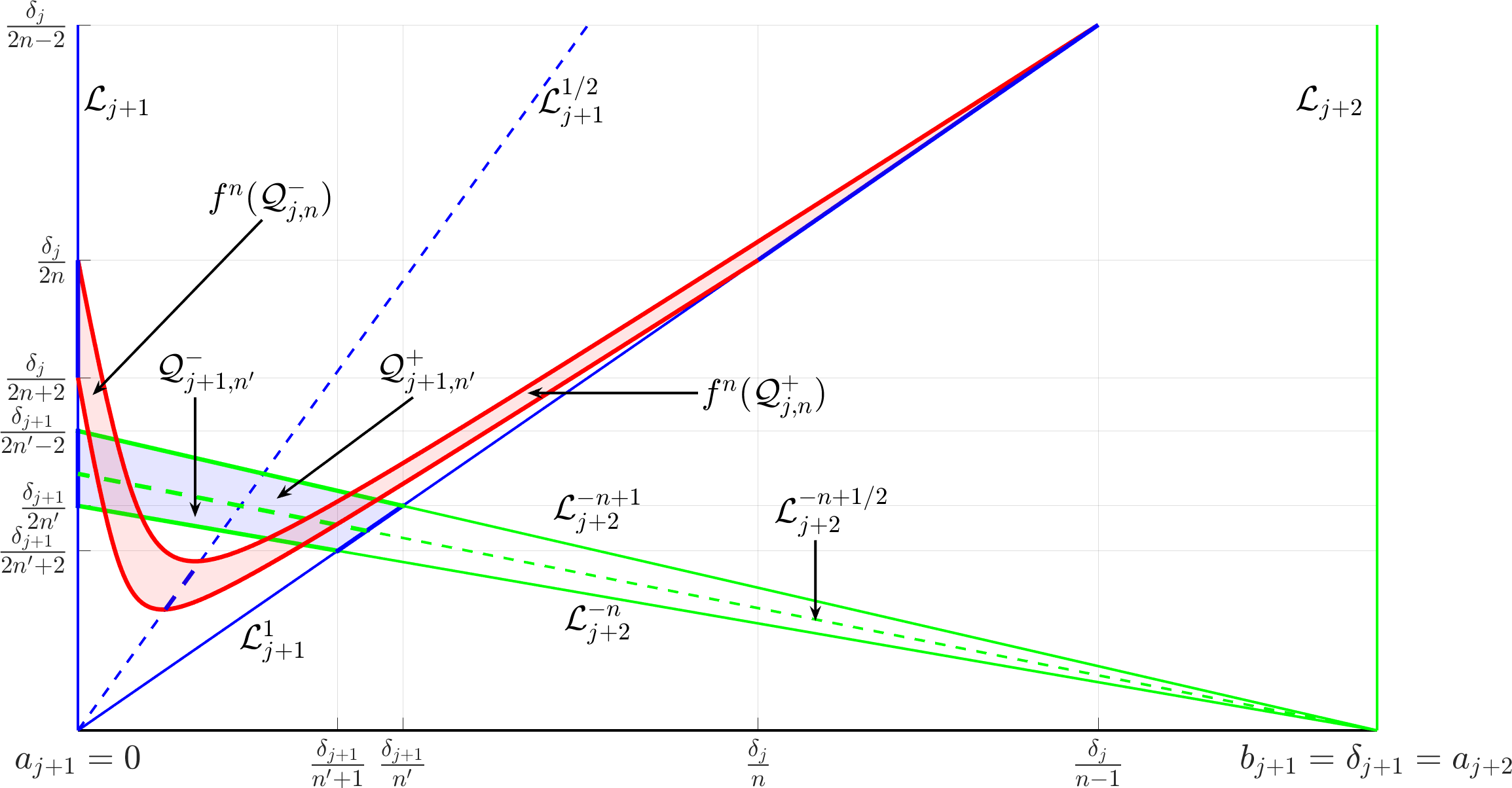
Figure 5: Overlapping of the image under $f^{n}$ of the fundamental quadrilateral $\mathcal{Q}_{j,n}=\mathcal{Q}^{-}_{j,n}\cup\mathcal{Q}^{+}_{j,n}$ displayed in Figure 4 with the ‘target’ fundamental quadrilateral $\mathcal{Q}_{j+1,n^{\prime}}=\mathcal{Q}^{-}_{j+1,n^{\prime}}\cup\mathcal{Q}^{+}_{j+1,n^{\prime}}$ in the case $\mu_{j}<1$. Singularity segments $\mathcal{L}^{s}_{j+1}$ and $\mathcal{L}^{-t}_{j+2}$ are displayed in blue and green, respectively. Besides, they are displayed with continuous and dashed lines when $s,t\in\mathbb{N}$ and $t\in\mathbb{N}+\frac{1}{2}$, respectively. The upper and lower red thick continuous curves are the images of the left and right sides of $\mathcal{Q}_{j,n}$, respectively. We have assumed that $a_{j+1}=0$ to avoid the overlapping of labels in the horizontal axis. This is a quantitative representation computed for $\delta_{j}=\pi/2$, $\delta_{j+1}=1$, $\mu_{j}=\sqrt{r_{j}/r_{j+1}}=0.3$, $n=3$ and $n^{\prime}=4$, showing that $f^{n}:\widetilde{\mathcal{Q}}^{\varsigma}_{j,n}\rightsquigarrow\widetilde{\mathcal{Q}}^{\varsigma^{\prime}}_{j+1,n^{\prime}}$ for all $\varsigma,\varsigma^{\prime}\in\{-,+\}$. The parabolic-like shape of $f^{n}(\mathcal{Q}_{j,n})$ was expected, see (6).

Proof.

We fix an index $j\mod k$ such that $\mu_{j}<1$, so $\alpha^{-}_{j}=\delta_{j+1}/\delta_{j}$ and $\alpha_{j}^{+}=\delta_{j+1}/\mu_{j}\delta_{j}$. Let $(n,n^{\prime})\in\Upsilon_{j}$. We want to show that $f^{n}:\widetilde{\mathcal{Q}}^{\varsigma}_{j,n}\rightsquigarrow\widetilde{\mathcal{Q}}^{\varsigma^{\prime}}_{j+1,n^{\prime}}$ for any $\varsigma,\varsigma^{\prime}\in\{-,+\}$.

Let $\gamma^{\varsigma}:[a,b]\to\mathcal{Q}^{\varsigma}_{j,n}$ be a path vertical in $\widetilde{Q}^{\varsigma}_{j,n}$. We assume, without loss of generality, that $\gamma^{\varsigma}(a)$ and $\gamma^{\varsigma}(b)$ belong to the base side and top side of $\tilde{\mathcal{Q}}^{\varsigma}_{j,n}$. Note that $\overline{\mathcal{D}_{j+1}\setminus\mathcal{Q}_{j+1,n^{\prime}}}$ has a connected component above and other one below $\mathcal{Q}_{j+1,n^{\prime}}$. By continuity and using that $\mathcal{Q}^{\varsigma^{\prime}}_{j+1,n^{\prime}}\subset\mathcal{Q}_{j+1,n^{\prime}}$ and $f^{n}(\gamma^{\varsigma})\subset\mathcal{D}_{j+1}$, we know that if $f^{n}(\gamma^{\varsigma}(a))$ and $f^{n}(\gamma^{\varsigma}(b))$ are in different connected components of $\overline{\mathcal{D}_{j+1}\setminus\mathcal{Q}_{j+1,n^{\prime}}}$, then there is a subpath $\eta^{\varsigma,\varsigma^{\prime}}\subset\gamma^{\varsigma}$ such that the image path $f^{n}(\eta^{\varsigma,\varsigma^{\prime}})$ is vertical in $\widetilde{\mathcal{Q}}^{\varsigma^{\prime}}_{j+1,n^{\prime}}$. Thus, we only have to check that endpoints $f^{n}(\gamma^{\varsigma}(a))$ and $f^{n}(\gamma^{\varsigma}(b))$ are in different connected components of $\overline{\mathcal{D}_{j+1}\setminus\mathcal{Q}_{j+1,n^{\prime}}}$ for any path $\gamma^{\varsigma}$ vertical in $\widetilde{Q}^{\varsigma}_{j,n}$.

First, we consider the case $\varsigma=-$, so $\gamma^{-}(a)\in\mathcal{Q}^{-}_{j,n}\cap\mathcal{L}^{-n}_{j+1}$ and $\gamma^{-}(b)\in\mathcal{Q}^{-}_{j,n}\cap\mathcal{L}^{-n+1/2}_{j+1}$. We deduce from Lemma 17 that

$$\Pi_{\theta}(f^{n}(\gamma^{-}(a))) \geq\min_{x\in\mathcal{Q}^{-}_{j,n}\cap\mathcal{L}^{-n}_{j+1}}\Pi_{\theta}(f^{n}(x))=\min_{x\in\mathcal{Q}_{j,n}\cap\mathcal{L}^{-n}_{j+1}}\Pi_{\theta}(f^{n}(x))=\delta_{j}/(2n+2),$$

$$\Pi_{\theta}(f^{n}(\gamma^{-}(b))) \leq\max_{x\in\mathcal{Q}^{-}_{j,n}\cap\mathcal{L}^{-n+1/2}_{j+1}}\Pi_{\theta}(f^{n}(x))<\mu_{j}\delta_{j}/(2n-1).$$

The above results and identities $\nu_{j+1,n^{\prime}}=\delta_{j+1}/(2n^{\prime}+2)$ and $\omega_{j+1,n^{\prime}}=\delta_{j+1}/(2n^{\prime}-2)$ imply that if inequalities

$$\mu_{j}\delta_{j}/(2n-1)\leq\delta_{j+1}/(2n^{\prime}+2),\qquad\delta_{j+1}/(2n^{\prime}-2)\leq\delta_{j}/(2n+2)$$ (9)

hold, then $f^{n}(\gamma^{-}(a))$ and $f^{n}(\gamma^{-}(b))$ are above and below $\mathcal{Q}_{j+1,n^{\prime}}$, respectively, so they are in different connected components of $\overline{\mathcal{D}_{j+1}\setminus\mathcal{Q}_{j+1,n^{\prime}}}$ for any path $\gamma^{-}$ vertical in $\widetilde{Q}^{-}_{j,n}$.

Second, we consider the case $\varsigma=+$, so $\gamma^{+}(a)\in\mathcal{Q}^{+}_{j,n}\cap\mathcal{L}^{-n+1/2}_{j+1}$ and $\gamma^{+}(b)\in\mathcal{Q}^{+}_{j,n}\cap\mathcal{L}^{-n+1}_{j+1}$. Similar arguments show that if inequalities

$$\mu_{j}\delta_{j}/(2n-1)\leq\delta_{j+1}/(2n^{\prime}+2),\qquad\delta_{j+1}/(2n^{\prime}-2)\leq\delta_{j}/2n$$ (10)

hold, then $f^{n}(\gamma^{+}(a))$ and $f^{n}(\gamma^{+}(b))$ are below and above $\mathcal{Q}_{j+1,n^{\prime}}$, respectively, so they are in different connected components of $\overline{\mathcal{D}_{j+1}\setminus\mathcal{Q}_{j+1,n^{\prime}}}$ for any path $\gamma^{+}$ vertical in $\widetilde{Q}^{+}_{j,n}$.

Finally, after a straightforward algebraic manipulation, we check that inequalities (9) and (10) hold for any $(n,n^{\prime})\in\Upsilon_{j}$. This ends the proof for the case $\mu_{j}<1$.

The case $\mu_{j}>1$ follows from similar arguments. We skip the details. ∎

No inequality in (8) is strict. However, we need some strict inequalities for a technical reason. Let us explain it. We will use the objects defined above and the fundamental lemma to construct our symbolic dynamics in Section 6. However, if we were to try to construct our symbolic dynamics directly with the symbol sets being the fundamental quadrilaterals $Q^{\varsigma}_{j,n}$, we would run into problems at the boundaries, where neighboring quadrilaterals intersect. To be precise, $\mathcal{Q}^{+}_{j,n}$ and $\mathcal{Q}^{-}_{j,n}$ have a common side contained in $\mathcal{L}_{j}^{-n+1/2}$, whereas $\mathcal{Q}^{-}_{j,n}$ and $\mathcal{Q}^{+}_{j,n+1}$ have a common side contained in $\mathcal{L}_{j}^{-n}$. The following corollary to Lemma 18 solves this problem by establishing the existence of pairwise disjoint strict horizontal slabs $\widetilde{\mathcal{K}}^{\varsigma}_{j,n}\varsubsetneq_{\rm h}\widetilde{\mathcal{Q}}^{\varsigma}_{j,n}$ with exactly the same stretching properties as the original fundamental quadrilaterals $\widetilde{\mathcal{Q}}^{\varsigma}_{j,n}$. It requires some strict inequalities.

Corollary 19 (Fundamental Corollary).

With the above notations, let

$$\Xi_{j}=\left\{(n,n^{\prime})\in\mathbb{N}^{2}:\alpha_{j}^{-}n+\beta_{j}^{-}<n^{\prime}<\alpha_{j}^{+}n-\beta_{j}^{+},\ n\geq\chi_{j},\ n^{\prime}\geq\chi_{j+1}\right\},$$

where $\alpha_{j}^{-}=\delta_{j+1}/\delta_{j}\max\{1,\mu_{j}\}$, $\alpha_{j}^{+}=\delta_{j+1}/\delta_{j}\min\{1,\mu_{j}\}$ and $\beta_{j}^{\pm}=\alpha_{j}^{\pm}+1$ for all $j\mod k$. There are pairwise disjoint strict horizontal slabs

$$\widetilde{\mathcal{K}}^{\varsigma}_{j,n}\varsubsetneq_{\rm h}\widetilde{\mathcal{Q}}^{\varsigma}_{j,n},\qquad\forall j\mod k,\ n\geq\chi_{j},\ \varsigma\in\{-,+\},$$

such that:

1. $f^{n}:\widetilde{\mathcal{K}}^{\varsigma}_{j,n}\rightsquigarrow\widetilde{\mathcal{K}}^{\varsigma^{\prime}}_{j+1,n^{\prime}}$; and

2. $f^{n}(\mathcal{K}^{\varsigma}_{j,n})\cap\mathcal{K}^{\varsigma^{\prime}}_{j+1,n^{\prime}}\cap\mathcal{L}=\emptyset$,

for all $j\mod k$, $(n,n^{\prime})\in\Xi_{j}$ and $\varsigma,\varsigma^{\prime}\in\{-,+\}$. (See Definition 12 for the meaning of $\mathcal{L}$.)

Proof.

Inequalities (9) and (10) become strict for any $(n,n^{\prime})\in\Xi_{j}$. We consider the oriented cells $\widetilde{\mathcal{R}}_{j+1,n}$, where

$$\mathcal{R}_{j+1,n}=\bigcup_{(n,n^{\prime})\in\Xi_{j}}\mathcal{Q}_{j+1,n^{\prime}}\subset\mathcal{D}_{j+1},$$

and orientations are chosen in such a way that the left and right sides of these big oriented cells are still contained in $\mathcal{L}_{j+1}$ and $\mathcal{L}_{j+1}^{1}$, respectively. Note that $\mathcal{D}_{j+1}\setminus\mathcal{R}_{j+1,n}$ has a connected component above and other one below $\mathcal{R}_{j+1,n}$.

Fix an index $j\mod k$ such that $\mu_{j}<1$. Let $n\geq\chi_{j}$. We refer to Figure 5 for a visual guide. The reader should imagine that the blue quadrilateral shown in that figure is our whole cell $\mathcal{R}_{j+1,n}$.

Strict versions of inequalities (9) and (10) imply that the images by $f^{n}$ of both the base side of $\widetilde{\mathcal{Q}}^{-}_{j,n}$ and the top side of $\widetilde{\mathcal{Q}}^{+}_{j,n}$ are strictly above $\mathcal{R}_{j+1,n}$; whereas the image by $f^{n}$ of the top side of $\widetilde{\mathcal{Q}}^{-}_{j,n}$, which coincides with the base side of $\widetilde{\mathcal{Q}}^{+}_{j,n}$, is strictly below $\mathcal{R}_{j+1,n}$. Thus, there are strict horizontal slabs $\widetilde{\mathcal{K}}^{\varsigma}_{j,n}\varsubsetneq_{\rm h}\widetilde{\mathcal{Q}}^{\varsigma}_{j,n}$, with $\varsigma\in\{-,+\}$, such that the images by $f^{n}$ of both the base side of $\widetilde{\mathcal{K}}^{-}_{j,n}$ and the top side of $\widetilde{\mathcal{K}}^{+}_{j,n}$ are strictly above $\mathcal{R}_{j+1,n}$; whereas the image by $f^{n}$ of both the top side of $\widetilde{\mathcal{K}}^{-}_{j,n}$ and the base side of $\widetilde{\mathcal{K}}^{+}_{j,n}$ are strictly below $\mathcal{R}_{j+1,n}$. Consequently, $f^{n}(\mathcal{K}^{\varsigma}_{j,n})\cap\mathcal{R}_{j+1,n}\cap\mathcal{L}=\emptyset$ and $f^{n}:\widetilde{\mathcal{K}}^{\varsigma}_{j,n}\rightsquigarrow\widetilde{\mathcal{R}}_{j+1,n}$, which implies that $f^{n}(\mathcal{K}^{\varsigma}_{j,n})\cap\mathcal{K}^{\varsigma^{\prime}}_{j+1,n^{\prime}}\cap\mathcal{L}=\emptyset$ and $f^{n}:\widetilde{\mathcal{K}}^{\varsigma}_{j,n}\rightsquigarrow\widetilde{\mathcal{K}}^{\varsigma^{\prime}}_{j+1,n^{\prime}}$ for all $(n,n^{\prime})\in\Xi_{j}$ and $\varsigma,\varsigma^{\prime}\in\{-,+\}$, since $\widetilde{\mathcal{K}}^{\varsigma^{\prime}}_{j+1,n^{\prime}}\subset_{\rm h}\widetilde{\mathcal{R}}_{j+1,n}$ for all $(n,n^{\prime})\in\Xi_{j}$ and $\varsigma^{\prime}\in\{-,+\}$. This ends the proof of the stretching and intersecting properties when $\mu_{j}<1$.

The case $\mu_{j}>1$ follows from similar arguments. We omit the details.

Finally, these strict horizontal slabs are necessarily pairwise disjoint because the original fundamental quadrilaterals $\widetilde{\mathcal{Q}}^{\varsigma}_{j,n}$ only share some of their horizontal sides. ∎

5 Symbols, shift spaces and shift maps

In this section, we define an alphabet $\boldsymbol{Q}\subset\mathbb{Z}^{k}$ with infinitely many symbols, then we consider two shift spaces $\mathfrak{Q}^{+}\subset\boldsymbol{Q}^{\mathbb{N}_{0}}$ and $\mathfrak{Q}\subset\boldsymbol{Q}^{\mathbb{Z}}$ of admissible one-sided and two-sided sequences, and finally we study some properties of the shift map $\sigma:\mathfrak{Q}\to\mathfrak{Q}$. We present these objects in a separate section, minimizing their relation with circular billiards, since we believe that they will be useful in future works about other problems.

For brevity, we will use the term shift instead of subshift, but $\mathfrak{Q}^{+}\varsubsetneq\boldsymbol{Q}^{\mathbb{N}_{0}}$ and $\mathfrak{Q}\varsubsetneq\boldsymbol{Q}^{\mathbb{Z}}$.

The sets $\boldsymbol{Q}$, $\mathfrak{Q}^{+}$ and $\mathfrak{Q}$ are defined in terms of some positive factors $\alpha^{\pm}_{j}$, some positive addends $\beta^{\pm}_{j}$ and some integers $\chi_{j}\geq 2$ for $j=1,\ldots,k$, with $k\geq 1$. (There are interesting billiard problems that will require $k<3$, or even $k=1$.)

We only assume three hypotheses about these factors and integers:

• $0<\alpha^{-}_{j}<\alpha^{+}_{j}$ for $j=1,\ldots,k$;

• $\alpha:=\alpha^{+}>1$ and $\alpha^{+}\alpha^{-}=1$, where $\alpha^{\pm}=\prod_{j=1}^{k}\alpha^{\pm}_{j}$; and

• Integers $\chi_{2},\ldots,\chi_{k}\geq 2$ are large enough and $\chi_{1}\gg\chi_{2},\ldots,\chi_{k}$.

There is no assumption on the addends. Factors $\alpha^{\pm}_{j}=\alpha^{\pm}_{j\mod k}$, addends $\beta^{\pm}_{j}=\beta^{\pm}_{j\mod k}$ and integers $\chi_{j}=\chi_{j\mod k}$ are extended cyclically. Clearly, all arcs $\Gamma_{1},\ldots,\Gamma_{k}$ of the circular polygon $\Gamma$ are equally important, so $\chi_{1}\gg\chi_{2},\ldots,\chi_{k}$ is a purely technical hypothesis. It is used only once, at the beginning of the proof of Lemma 24. It is needed just to establish the topological transitivity of the subshift map. The rest of Theorem A, as well as Theorems C, D and E do not need it.

We remark two facts related to billiards in circular polygons, although we forget about billiards in the rest of this section. The first remark is a trivial verification.

Lemma 20.

The factors $\alpha^{\pm}_{j}$ defined in Lemma 18 satisfy hypotheses (A) and (B).

Proof.

Hypothesis (A) follows from properties $\mu_{j}\neq 1$. Hypothesis (B) follows from the telescopic products

$$\prod_{j=1}^{k}\frac{\delta_{j}}{\delta_{j+1}}=1,\qquad\prod_{j=1}^{k}\mu_{j}=\prod_{j=1}^{k}\sqrt{\frac{r_{j}}{r_{j+1}}}=1,$$

which are easily obtained from the cyclic identities $\delta_{k+1}=\delta_{1}$ and $r_{k+1}=r_{1}$. ∎

The second remark is that we prefer to encode in a single symbol all information related to each complete turn around $\Gamma$, although we may construct our symbolic dynamics directly with the disjoints sets $\widetilde{\mathcal{K}}^{\varsigma}_{j,n}$ as symbols. That is, if a generic sliding orbit follows, along a complete turn around the boundary $\Gamma$, the itinerary

$$\mathcal{K}^{\varsigma_{1}}_{1,n_{1}}\subset\mathcal{D}_{1},\mathcal{K}^{\varsigma_{2}}_{2,n_{2}}\subset\mathcal{D}_{2},\ldots,\mathcal{K}^{\varsigma_{k}}_{k,n_{k}}\subset\mathcal{D}_{k},$$

where $\widetilde{\mathcal{K}}^{\varsigma}_{j,n}$ are the pairwise disjoint horizontal slabs described in Corollary 19, then we construct the symbol

$$\boldsymbol{q}=(q_{1},\ldots,q_{k})\in\mathbb{Z}^{k},\qquad|q_{j}|=n_{j},\qquad\mathop{\rm sign}\nolimits(q_{j})=\varsigma_{j},$$

which motivates the following definition.

Definition 21.

The alphabet of admissible symbols is the set

$$\boldsymbol{Q}=\left\{\boldsymbol{q}=(q_{1},\ldots,q_{k})\in\mathbb{Z}^{k}:\begin{array}[]{l}\alpha_{j}^{-}|q_{j}|+\beta_{j}^{-}<|q_{j+1}|<\alpha_{j}^{+}|q_{j}|-\beta_{j}^{+},\,\mbox{$\forall j=1,\ldots,k-1$}\\ |q_{j}|\geq\chi_{j},\mbox{ $\forall j=1,\ldots,k$}\end{array}\right\}.$$

This alphabet has infinitely many symbols by hypothesis (A). Thinking in the billiard motivation behind these symbols, we ask that symbols associated to consecutive turns around $\Gamma$ satisfy the following admissibility condition.

Definition 22.

We say that a finite, one-sided, or two-sided sequence of admissible symbols $\mathfrak{q}=(\boldsymbol{q}^{i})_{i\in I}\subset\boldsymbol{Q}$, with $\boldsymbol{q}^{i}=(q_{1}^{i},\ldots,q_{k}^{i})$, is admissible if and only if

$$\alpha_{k}^{-}|q^{i}_{k}|+\beta_{k}^{-}<|q^{i+1}_{1}|<\alpha_{k}^{+}|q^{i}_{k}|-\beta_{k}^{+},\qquad\forall i.$$

Admissible sequences are written with Fraktur font: $\mathfrak{q}$. Its vector symbols are written with boldface font and labeled with superscripts: $\boldsymbol{q}^{i}$. Components of admissible symbols are written with the standard font and labeled with subscripts: $q^{i}_{j}$ or $q_{j}$.

Definition 23.

The shift spaces of admissible sequences are

$$\mathfrak{Q}^{+} =\left\{\mathfrak{q}=(\boldsymbol{q}^{i})_{i\in\mathbb{N}_{0}}\in\boldsymbol{Q}^{\mathbb{N}_{0}}:\mbox{$\mathfrak{q}$ is admissible}\right\},$$

$$\mathfrak{Q} =\left\{\mathfrak{q}=(\boldsymbol{q}^{i})_{i\in\mathbb{Z}}\in\boldsymbol{Q}^{\mathbb{Z}}:\mbox{$\mathfrak{q}$ is admissible}\right\}.$$

If $\boldsymbol{q}=(q_{1},\ldots,q_{k})\in\boldsymbol{Q}$, then we write $|\boldsymbol{q}|=|q_{1}|+\cdots+|q_{k}|$. We equip $\mathfrak{Q}$ with the topology defined by the metric

$$d_{\mathfrak{Q}}:\mathfrak{Q}\times\mathfrak{Q}\to[0,+\infty),\qquad d_{\mathfrak{Q}}(\mathfrak{p},\mathfrak{q})=\sum_{i\in\mathbb{Z}}\frac{1}{2^{|i|}}\frac{|\boldsymbol{p}^{i}-\boldsymbol{q}^{i}|}{1+|\boldsymbol{p}^{i}-\boldsymbol{q}^{i}|}.$$

We want to estimate the size of the maxima (sometimes, the minima as well) of the sets

$$\Xi^{i}_{j}(n)=\left\{n^{i}_{j}\in\mathbb{N}:\exists\mathfrak{q}\in\mathfrak{Q}\mbox{ such that $|q^{0}_{1}|=n$ and $|q^{i}_{j}|=n^{i}_{j}$}\right\},\quad i\in\mathbb{Z},\ j=1,\ldots,k,$$ (11)

when $n\geq\chi_{1}$ or $n\gg 1$. We ask in (11) for the existence of some $\mathfrak{q}\in\mathfrak{Q}$ —that is, some two-sided infinite sequence—, but it does not matter. We would obtain exactly the same sets just by asking the existence of some finite sequence $q^{0}_{1},\ldots,q^{0}_{k},q^{1}_{1},\ldots,q^{1}_{k},\ldots,q^{i}_{1},\ldots,q^{i}_{j}$ that satisfies the corresponding admissibility conditions.

Several estimates about maxima and minima of sets (11) are listed below. Their proofs have been postponed to Appendix A.

Lemma 24.

We assume hypotheses (A), (B) and (X). Set $\zeta^{i}_{j}(n)=\min\Xi^{i}_{j}(n)$, $\xi^{i}_{j}(n)=\max\Xi^{i}_{j}(n)$. Let $\rho^{0}(n)=n$ and $\rho^{i}(n)=\sum_{j=1}^{k}\sum_{m=0}^{i-1}\xi^{m}_{j}(n)$ for all $i\geq 1$.

1. There are positive constants $\nu<\lambda$, $\nu^{\prime}<\lambda^{\prime}$, $\tau<1$ and $\gamma^{\pm}$, which depend on factors $\alpha^{\pm}_{j}$ and addends $\beta^{\pm}_{j}$ but not on integers $\chi_{j}$, such that the following properties hold.

   1. $\nu n\leq\xi^{0}_{j}(n)\leq\lambda n$ for all $j=1,\ldots,k$ and $n\geq\chi_{1}$;

   2. $\tau\alpha^{|i|}\xi^{0}_{j}(n)\leq\xi^{i}_{j}(n)\leq\alpha^{|i|}\xi^{0}_{j}(n)$ for all $j=1,\ldots,k$, $i\in\mathbb{Z}$ and $n\geq\chi_{1}$;

   3. $\nu^{\prime}\xi_{j}^{i}(n)\leq\rho^{i}(n)\leq\rho^{i+1}(n)\leq\lambda^{\prime}\xi_{j}^{i}(n)$ for all $j=1,\ldots,k$, $i\geq 0$, and $n\geq\chi_{1}$;

   4. $\zeta^{1}_{1}(n)\leq\max\{\chi_{1},n/\alpha+\gamma^{-}\}\leq n-1<n+1\leq\alpha n-\gamma^{+}\leq\xi^{1}_{1}(n)$ for all $n>\chi_{1}$ and $\zeta^{1}_{1}(n)=n<n+1\leq\alpha n-\gamma^{+}\leq\xi^{1}_{1}(n)$ for $n=\chi_{1}$; and

   5. Once fixed any $N\in\mathbb{N}$, we have that

      $$\chi_{1}\leq\zeta^{1}_{1}(n)\leq n/\alpha+\gamma^{-}\leq n-N<n+N\leq\alpha n-\gamma^{+}\leq\xi^{1}_{1}(n),\quad\forall n\gg 1.$$

2. $\Xi^{i}_{j}(n)=[\zeta^{i}_{j}(n),\xi^{i}_{j}(n)]\cap\mathbb{N}$ for all $j\mod k$, $i\in\mathbb{Z}$ and $n\geq\chi_{1}$; that is, $\Xi^{i}_{j}(n)$ has no gaps in $\mathbb{N}$. Besides, $\big{[}\max\{\chi_{1},n-|i|\},n+|i|\big{]}\cap\mathbb{N}\subset\Xi^{i}_{1}(n)$ for all $i\in\mathbb{Z}$ and $n\geq\chi_{1}$.

Corollary 25.

We assume hypotheses (A), (B) and (X).

1. Given any $\boldsymbol{q}^{-},\boldsymbol{q}^{+}\in\boldsymbol{Q}$ there is an admissible sequence of the form $\big{(}\boldsymbol{q}^{-},\boldsymbol{q}^{1},\ldots,\boldsymbol{q}^{l},\boldsymbol{q}^{+}\big{)}$ for some $l\in\mathbb{N}$ and $\boldsymbol{q}^{1},\ldots,\boldsymbol{q}^{l}\in\boldsymbol{Q}$.

2. Given any $N\in\mathbb{N}$, there is a subset $\boldsymbol{Q}_{N}\subset\boldsymbol{Q}$, with $\#\boldsymbol{Q}_{N}=N$, such that the short sequence $(\boldsymbol{q},\boldsymbol{q}^{\prime})$ is admissible for all $\boldsymbol{q},\boldsymbol{q}^{\prime}\in\boldsymbol{Q}_{N}$.

3. $\mathfrak{Q}\neq\emptyset$.

Proof.

1. Let $l=|q^{-}_{1}-q^{+}_{1}|-1$. Part (b) of Lemma 24 implies that $q^{+}_{1}\in\Xi^{l+1}_{1}(q^{-}_{1})$. Therefore, we can construct iteratively such a sequence $\boldsymbol{q}^{1},\ldots,\boldsymbol{q}^{l}$.

2. Fix $N\in\mathbb{N}$. Part (av) of Lemma 24 implies that if $\boldsymbol{q},\boldsymbol{q}^{\prime}\in\boldsymbol{Q}$ with $|q_{1}-q^{\prime}_{1}|\leq N$ and $|q_{1}|,|q^{\prime}_{1}|\gg 1$, then $(\boldsymbol{q},\boldsymbol{q}^{\prime})$ is admissible. So, we can take any subset $\boldsymbol{Q}_{N}=\{\boldsymbol{q}^{1},\ldots,\boldsymbol{q}^{N}\}\subset\boldsymbol{Q}$ such that $|q_{1}^{n}|=|q^{1}_{1}|+n-1$ with $|q_{1}^{1}|\gg 1$. Clearly, $\#\boldsymbol{Q}_{N}=N$.

3. Let $\mathfrak{q}=(\boldsymbol{q}^{i})_{i\in\mathbb{Z}}$ with $\boldsymbol{q}^{i}=(q_{1}^{i},\ldots,q_{k}^{i})\in\boldsymbol{Q}$ such that $|q_{1}^{i+1}-q_{1}^{i}|\leq 1$. Then $\mathfrak{q}\in\mathfrak{Q}$. ∎

Definition 26.

The shift map $\sigma:\mathfrak{Q}\to\mathfrak{Q}$, $\mathfrak{p}=\sigma(\mathfrak{q})$, is given by $\mathfrak{p}^{i}=\mathfrak{q}^{i+1}$ for all $i\in\mathbb{Z}$.

The following proposition tells us some important properties of the shift map. Note that by topological transitivity we mean for any nonempty open sets $U,V\subset\mathfrak{Q}$ there is $n\in\mathbb{N}$ such that $\sigma^{n}(U)\cap V\neq\emptyset$. If $N\in\mathbb{N}$, $\Sigma_{N}=\{1,\ldots,N\}^{\mathbb{Z}}$ and the shift map $\sigma_{N}:\Sigma_{N}\to\Sigma_{N}$, $(t_{i})_{i\in\mathbb{Z}}=\sigma_{N}\big{(}(s_{i})_{i\in\mathbb{Z}}\big{)}$, is given by $t_{i}=s_{i+1}$ for all $i\in\mathbb{Z}$, then we say that $\sigma_{N}:\Sigma_{N}\to\Sigma_{N}$ is the full $N$-shift. We denote by $h_{\rm top}(f)$ the topological entropy of a continuous self-map $f$.

Proposition 27.

We assume hypotheses (A), (B) and (X).

The shift map $\sigma:\mathfrak{Q}\to\mathfrak{Q}$ exhibits topological transitivity and sensitive dependence on initial conditions, has infinite topological entropy, and contains the full $N$-shift as a topological factor for any $N\in\mathbb{N}$. Besides, the subshift space of periodic admissible sequences

$$\mathfrak{P}=\left\{\mathfrak{q}=\mathfrak{Q}:\mbox{$\exists p\in\mathbb{N}$ such that $\sigma^{p}(\mathfrak{q})=\mathfrak{q}$}\right\}$$

is dense in the shift space $\mathfrak{Q}$.

Proof.

On the one hand, part (a) of Corollary 25 implies that the shift map $\sigma:\mathfrak{Q}\to\mathfrak{Q}$ is equivalent to a transitive topological Markov chain. It is well-known that such objects exhibit topological transitivity, sensitive dependence on initial conditions, and density of periodic points. See, for example, Sections 1.9 and 3.2 of [39].

On the other hand, let $\boldsymbol{Q}_{N}=\{\boldsymbol{q}^{1},\ldots,\boldsymbol{q}^{N}\}$ be the set provided in part (b) of Corollary 25. Set $\mathfrak{Q}_{N}=(\boldsymbol{Q}_{N})^{\mathbb{Z}}$. We consider the bijection

$$g=(g^{i})_{i\in\mathbb{Z}}:\mathfrak{Q}_{N}\to\Sigma_{N},\quad g^{i}(\boldsymbol{q}^{n})=n,\qquad\forall i\in\mathbb{Z},\ \forall n\in\{1,\ldots,N\}.$$

Then $\mathfrak{Q}_{N}$ is a subshift space of $\mathfrak{Q}$. That is, $\sigma(\mathfrak{Q}_{N})=\mathfrak{Q}_{N}$. Besides, the diagram

commutes, so $h_{\rm top}(\sigma)\geq h_{\rm top}(\sigma_{|\mathfrak{Q}_{N}})=h_{\rm top}(\sigma_{N})=\log N$ for all $N\in\mathbb{N}$. This means that $\sigma$ has infinite topological entropy. ∎

6 Chaotic motions

In this section, we detail the construction of a domain accumulating on the boundary of the phase space on which the dynamics is semiconjugate to a shift on infinitely many symbols, thus proving Theorem A; in fact, we reformulate Theorem A in the form of Theorem 31 below. The proof uses the method of stretching along the paths summarized in Section 3, the fundamental corollary obtained in Section 4 and the shift map described in Section 5.

First, we list all notations and conventions used along this section. Let $\Gamma$ be a circular $k$-gon with arcs $\Gamma_{j}$, radii $r_{j}$ and central angles $\delta_{j}$. Set $\mu_{j}=\sqrt{r_{j}/r_{j+1}}$. Then $\alpha^{\pm}_{j}$, $\beta^{\pm}_{j}=\alpha_{j}^{\pm}+1$ and $\chi_{j}\geq 2$ are the factors, addends and integers introduced in Lemma 17 and Corollary 19. These factors satisfy hypotheses (A) and (B). Besides, we assume hypothesis (X), so Proposition 27 holds. The index $j$ is defined modulo $k$. Let $\mathcal{M}=\mathbb{T}\times[0,\pi]$ be the phase space of the billiard map $f:\mathcal{M}\to\mathcal{M}$. Let $\mathcal{S}_{0}$ be the generic sliding set, see Definition 13. Let $\widetilde{\mathcal{K}}^{\varsigma}_{j,n}$, with $\mathcal{K}^{\varsigma}_{j,n}\subset\mathcal{D}_{j}$, be the pairwise disjoint oriented cells introduced in Corollary 19, where $j\mod k$, $n\in\mathbb{N}$ with $n\geq\chi_{j}$ and $\varsigma\in\{-,+\}$. Let $\sigma:\mathfrak{Q}\to\mathfrak{Q}$ be the shift map studied in Section 5. Finally, the reader should be aware of the conventions about calligraphic, Fraktur, boldface and standard fonts.

Definition 28.

Partial sums $s^{i},s^{i}_{j}:\mathfrak{Q}\to\mathbb{Z}$ for $i\in\mathbb{Z}$ and $j=1,\ldots,k$ are defined by

$$s^{i}(\mathfrak{q})=\begin{cases}\displaystyle\phantom{-}\sum_{m=0}^{i-1}\sum_{j=1}^{k}|q^{m}_{j}|,&\mbox{ for $i\geq 0$},\\ \displaystyle-\sum_{m=i}^{-1}\sum_{j=1}^{k}|q^{m}_{j}|,&\mbox{ for $i<0$},\end{cases}\qquad\qquad s^{i}_{j}(\mathfrak{q})=s^{i}(\mathfrak{q})+\sum_{m=1}^{j-1}|q^{i}_{m}|.$$

Partial sums $s^{i},s^{i}_{j}:\mathfrak{Q}^{+}\to\mathbb{N}_{0}$ are analogously defined for $i\geq 0$ and $j=1,\ldots,k$.

The following proposition gives the relationship between some types of admissible sequences (two-sided: $\mathfrak{q}\in\mathfrak{Q}$, one-sided: $\mathfrak{q}\in\mathfrak{Q}^{+}$ and periodic: $\mathfrak{q}\in\mathfrak{P}$) and orbits of $f$ with prescribed itineraries in the set of pairwise disjoint cells $\mathcal{K}^{\varsigma}_{j,n}$ with $j=1,\ldots,k$, $n\geq\chi_{j}$ and $\varsigma\in\{-,+\}$. It is the key step in obtaining chaotic properties.

Proposition 29.

We have the following three versions.

• If $\mathfrak{q}\in\mathfrak{Q}$, then there is $x\in\mathcal{D}_{1}$ such that

  $$f^{s^{i}_{j}(\mathfrak{q})}(x)\in\mathcal{K}^{\mathop{\rm sign}\nolimits(q^{i}_{j})}_{j,|q^{i}_{j}|},\qquad\forall i\in\mathbb{Z},\ \forall j=1,\ldots,k.$$ (12)

• If $\mathfrak{q}\in\mathfrak{Q}^{+}$, then there is a path $\gamma\subset\mathcal{D}_{1}$ such that:

  1. $f^{s^{i}_{j}(\mathfrak{q})}(\gamma)\subset\mathcal{K}^{\mathop{\rm sign}\nolimits(q^{i}_{j})}_{j,|q^{i}_{j}|}$ for all $i\geq 0$ and $j=1,\ldots,k$; and

  2. $\gamma$ is horizontal in $\mathcal{D}_{1}$ (that is, $\gamma$ connects the left side $\mathcal{L}_{1}$ with the right side $\mathcal{L}_{1}^{1}$).

• If $\mathfrak{q}\in\mathfrak{P}$ has period $p$, then there is a point $x\in\mathcal{D}_{1}$ such that:

  1. $f^{s^{i}_{j}(\mathfrak{q})}(x)\in\mathcal{K}^{\mathop{\rm sign}\nolimits(q^{i}_{j})}_{j,|q^{i}_{j}|}$ for all $i\in\mathbb{Z}$ and $j=1,\ldots,k$; and

  2. $f^{s^{p}(\mathfrak{q})}(x)=x$, so $x$ is a $(p,s^{p}(q))$-periodic point of $f$ with period $s^{p}(\mathfrak{q})$ and rotation number $p/s^{p}(\mathfrak{q})$.

All these billiard orbits are contained in the generic sliding set $\mathcal{S}_{0}$. In particular, they have no points in the extended singularity set $\mathcal{L}=\bigcup_{j}\left(\mathcal{L}_{j}\cup\mathcal{L}_{j}^{1/2}\cup\mathcal{L}_{j}^{1}\right)$. Obviously, these claims only hold for forward orbits in version (O).

Proof.

It is a direct consequence of Theorem 9, Corollary 19, the definitions of admissible symbols and admissible sequences, and the definition of rotation number. ∎

To adapt the language of [49, 50, 52] to our setting, one could say that Proposition 29 implies that the billiard map induces chaotic dynamics on infinitely many symbols.

Remark 30.

The partial sum $s^{i}(\mathfrak{q})$, with $i\geq 0$, introduced in Definition 28 counts the number of impacts that any of its corresponding sliding billiard trajectories have after the first $i$ turns around $\Gamma$. Analogously, $s^{i}_{j}(\mathfrak{q})$, with $i\geq 0$, adds to the previous count the number of impacts in the first $j-1$ arcs at the $(i+1)$-th turn. There is no ambiguity in these counts, because generic sliding billiard trajectories have no impacts on the set of nodes $\Gamma_{\star}$, see Remark 14. The partial sums with $i<0$ store information about the backward orbit.

Let us introduce four subsets of the first fundamental domain that will be invariant under a return map $F$ yet to be defined. First, we consider the fundamental generic sliding set

$$\mathcal{R}=\mathcal{S}_{0}\cap\mathcal{D}_{1}\subset\mathop{\rm Int}\nolimits\mathcal{D}_{1}.$$

Any $f$-orbit that begins in $\mathcal{R}$ returns to $\mathcal{R}$ after a finite number of iterations of the billiard map $f$. Let $\tau:\mathcal{R}\to\mathbb{N}$ be the return time defined as $\tau(x)=\min\{n\in\mathbb{N}:f^{n}(x)\in\mathcal{R}\}$. Then $F:\mathcal{R}\to\mathcal{R}$, $F(x)=f^{\tau(x)}(x)$, is the promised return map. The return map $F:\mathcal{R}\to\mathcal{R}$ is a homeomorphism since the billiard map $f:\mathcal{M}\to\mathcal{M}$ is a homeomorphism and $\mathcal{R}$ is contained in the interior of the fundamental set $\mathcal{D}_{1}$.

Next, we define the sets

$$\mathcal{I} =\big{\{}x\in\mathcal{M}:\mbox{$\exists\mathfrak{q}\in\mathfrak{Q}$ such that the prescribed itinerary~{}\eqref{eq:PrescribedItinerary} takes place}\big{\}},$$

$$\mathcal{P} =\big{\{}x\in\mathcal{I}:\mbox{$\exists p\in\mathbb{N}$ such that $F^{p}(x)=x$}\big{\}}$$

and the map $h:\mathcal{I}\to\mathfrak{Q}$, $h(x)=\mathfrak{q}$, where $\mathfrak{q}$ is the unique admissible sequence such that the prescribed itinerary (12) takes place. It is well-defined because cells $\mathcal{K}_{j,n}^{\varsigma}$ are pairwise disjoint. This is the topological semiconjugacy we were looking for. Clearly,

$$\tau(x)=s^{1}(\mathfrak{q})=|q^{0}_{1}|+\cdots+|q^{0}_{k}|,\qquad\forall x\in\mathcal{I},\ \mathfrak{q}=h(x)$$ (13)

where $\tau(x)$ is the return time and the partial sum $s^{1}(\mathfrak{q})$ counts the number of impacts after the first turn around $\Gamma$ of the billiard orbit starting at $x$.

Theorem 31.

The sets $\mathcal{P}$, $\mathcal{J}:=\overline{\mathcal{P}}$, $\mathcal{I}$ and $\mathcal{R}$ are $F$-invariant:

$$F(\mathcal{P})=F(\mathcal{P}),\qquad F(\mathcal{J})=F(\mathcal{J}),\qquad F(\mathcal{I})\subset\mathcal{I},\qquad F(\mathcal{R})=F(\mathcal{R}).$$

Besides, $\emptyset\neq\mathcal{P}\varsubsetneq\mathcal{J}\subset\mathcal{I}\subset\mathcal{R}$. The maps $h:\mathcal{I}\to\mathfrak{Q}$, $h_{|\mathcal{J}}:\mathcal{J}\to\mathfrak{Q}$ and $h_{|\mathcal{P}}:\mathcal{P}\to\mathfrak{P}$ are continuous surjections, and the three diagrams

                         (14)

commute. Periodic points of $F_{|\mathcal{J}}$ are dense in $\mathcal{J}$. Given any $\mathfrak{q}\in\mathfrak{P}$ with period $p$, there is at least one $x\in(h_{|\mathcal{P}})^{-1}(\mathfrak{q})\in\mathcal{P}$ such that $f^{s^{p}(\mathfrak{q})}(x)=F^{p}(x)=x$.

Proof.

Properties $F(\mathcal{P})=\mathcal{P}$, $F(\mathcal{R})=\mathcal{R}$ and $\mathcal{P}\subset\mathcal{I}$ are trivial, by construction. Inclusion $\mathcal{I}\subset\mathcal{R}$ follows from the definitions of both sets and property (b) of Corollary 19.

Let us prove that $h:\mathcal{I}\to\mathfrak{Q}$ is continuous and surjective. Surjectivity follows directly from version (T) of Proposition 29. Choose any $x\in\mathcal{I}$ and $\epsilon>0$. Choose $l\in\mathbb{N}$ such that $\sum_{|i|>l}2^{-|i|}<\epsilon$. Let $\mathfrak{q}=(\boldsymbol{q}^{i})_{i\in\mathbb{Z}}=h(x)$ with $\boldsymbol{q}^{i}=(q_{1}^{i},\ldots,q_{k}^{i})$. Using that the compact sets $\mathcal{K}_{j,n}^{\varsigma}$ are mutually disjoint, $F$ is a homeomorphism and condition (12), we can find $\delta_{j}^{i}>0$ for each $|i|\leq l$ and $j=1,\ldots,k$ such that

$$f^{s^{i}_{j}(\mathfrak{q})}\big{(}\mathcal{B}_{\delta_{j}^{i}}(x)\cap\mathcal{I}\big{)}\subset\mathcal{K}^{\mathop{\rm sign}\nolimits(q^{i}_{j})}_{j,|q^{i}_{j}|},\qquad\forall|i|\leq l,\ \forall j=1,\ldots,k.$$

Here, $\mathcal{B}_{\delta}(x)$ is the disc of radius $\delta$ centered at $x$. If $\delta=\min\{\delta_{j}^{i}:|i|\leq l,\ j=1,\ldots,k\}$, then

$$\mbox{$d(x,y)<\delta$ and $\mathfrak{p}=(\boldsymbol{p}^{i})_{i\in\mathbb{Z}}=h(y)\Longrightarrow\boldsymbol{p}^{i}=\boldsymbol{q}^{i}$ for each $|i|\leq l$}.$$

Therefore,

$$d_{\mathfrak{Q}}\big{(}h(y),h(x)\big{)}=d_{\mathfrak{Q}}(\mathfrak{p},\mathfrak{q})=\sum_{|i|>l}\frac{1}{2^{|i|}}\frac{|\boldsymbol{p}^{i}-\boldsymbol{q}^{i}|}{1+|\boldsymbol{p}^{i}-\boldsymbol{q}^{i}|}<\sum_{|i|>l}\frac{1}{2^{|i|}}<\epsilon,$$

which implies that $h:\mathcal{I}\to\mathfrak{Q}$ is continuous.

Next, we prove simultaneously that $F(\mathcal{I})\subset\mathcal{I}$ and that $\sigma\circ h=h\circ F_{|\mathcal{I}}$. Let $x\in\mathcal{I}$, $y=F(x)\in\mathcal{R}$, $\mathfrak{q}=(\boldsymbol{q}^{i})_{i\in\mathbb{Z}}=h(x)$ with $\boldsymbol{q}^{i}=(q_{1}^{i},\ldots,q_{k}^{i})$, and $\mathfrak{p}=(\boldsymbol{p}^{i})_{i\in\mathbb{Z}}=\sigma(\mathfrak{q})\in\mathfrak{Q}$ with $\boldsymbol{p}^{i}=(p_{1}^{i},\ldots,p_{k}^{i})$, so $\boldsymbol{p}^{i}=\boldsymbol{q}^{i+1}$ and $p_{j}^{i}=q_{j}^{i+1}$. The prescribed itinerary (12) and relation (13) imply that

$$f^{s^{i}_{j}(\mathfrak{p})}(y)=f^{s^{i}_{j}(\sigma(\mathfrak{q}))}(F(x))=f^{s^{i+1}_{j}(\mathfrak{q})-s^{1}(\mathfrak{q})}\big{(}f^{s^{1}(\mathfrak{q})}(x)\big{)}=f^{s^{i+1}_{j}(\mathfrak{q})}(x)\in\mathcal{K}^{\mathop{\rm sign}\nolimits(q^{i+1}_{j})}_{j,|q^{i+1}_{j}|}=\mathcal{K}^{\mathop{\rm sign}\nolimits(p^{i}_{j})}_{j,|p^{i}_{j}|}$$

for all $i\in\mathbb{Z}$ and $j=1,\ldots,k$, so $\sigma(h(x))=\sigma(\mathfrak{q})=\mathfrak{p}=h(y)=\sigma(F(x))$ and $F(x)=y\in h^{-1}(\mathfrak{p})\subset\mathcal{I}$ for all $x\in\mathcal{I}$, as we wanted to prove. Hence, the first diagram in (14) defines a topological semiconjugacy.

Let us check that $\mathcal{J}:=\overline{\mathcal{P}}\subset\mathcal{I}$ and $F(\mathcal{J})=\mathcal{J}$. We have $\mathcal{J}\subset\mathcal{I}$, because $\mathcal{I}=h^{-1}(\mathfrak{Q})$ is closed (continuous preimage of a closed set). Besides, on one hand we have $\mathcal{P}=F(\mathcal{P})\subset F(\overline{\mathcal{P}})=F(\mathcal{J})$ implying that $\mathcal{J}=\overline{\mathcal{P}}\subset\overline{F(\mathcal{J})}=F(\mathcal{J})$, while on the other we have $F(\mathcal{J})=F(\overline{\mathcal{P}})\subset\overline{F(\mathcal{P})}=\overline{\mathcal{P}}=\mathcal{J}$. To establish that the second diagram in (14) is still a topological semiconjugacy, we must prove that $h(\mathcal{J})=\mathfrak{Q}$. We clearly have $h(\mathcal{J})\subset\mathfrak{Q}$ since $\mathcal{J}\subset\mathcal{I}$, and since $h_{|\mathcal{I}}$ is a semiconjugacy. Meanwhile, since $\mathcal{J}$ is compact (closed by definition and contained in the bounded set $\mathcal{D}_{1}$) so too is $h(\mathcal{J})$; moreover $h(\mathcal{J})$ contains $h(\mathcal{P})=\mathfrak{P}$ which is dense in $\mathfrak{Q}$ by Proposition 27, and so we obtain $\mathfrak{Q}=\overline{\mathfrak{P}}\subset h(\mathcal{J})$. Therefore $h(\mathcal{J})=\mathfrak{Q}$.

To complete the proof of the theorem, notice that periodic points of $F_{|\mathcal{J}}$ are dense in $\mathcal{J}$ by construction and the last claim of the Theorem 31 follows from version (P) of Proposition 29, which also implies $\mathcal{P}\neq\emptyset$. ∎

Proposition 27 and Theorem 31 imply Theorem A as stated in the introduction and it is the first step in proving Theorems C, D and E. For instance, upon combining Theorem 31 with the topological transitivity of the shift map guaranteed by Proposition 27, we already obtain the existence of trajectories approaching the boundary asymptotically. It remains to determine the optimal rate of diffusion. This is done in Section 7 by analyzing the sequences $\mathfrak{q}=(\boldsymbol{q}^{i})_{i\geq 0}\in\mathfrak{Q}^{+}$ for which $s^{i}(\mathfrak{q})$ increases in the fastest possible way as $i\to+\infty$. Lemma 24 plays a role in that analysis.

We end this section with three useful corollaries. First, we prove Corollary B on final sliding motions.

Proof of Corollary B.

The clockwise case is a by-product of the counter-clockwise one, because if we concatenate the arcs $\Gamma_{1},\ldots,\Gamma_{k}$ of the original circular polygon $\Gamma$ in the reverse order $\Gamma_{k},\ldots,\Gamma_{1}$, then we obtain the reversed circular polygon $\Gamma^{\prime}$ with the property that counter-clockwise sliding billiard trajectories in $\Gamma^{\prime}$ are in 1-to-1 correspondence with clockwise sliding billiard trajectories in $\Gamma$. Thus, it suffices to consider the counter-clockwise case.

Symbols $\boldsymbol{q}=(q_{1},\ldots,q_{k})\in\boldsymbol{Q}\subset\mathbb{Z}^{k}$ keep track of the proximity of the fundamental quadrilaterals $\mathcal{Q}_{j,|q_{j}|}$ to the inferior boundary of $\mathcal{M}$. That is, the larger the absolute value $|q_{j}|$, the smaller the angle of reflection $\theta$ for any $x=(\varphi,\theta)\in\mathcal{Q}_{j,|q_{j}|}$. For this reason, by construction, if one considers a bounded sequence in $\mathfrak{Q}$, (respectively, a sequence $\mathfrak{q}\in\mathfrak{Q}$ such that $\chi_{j}\leq\min_{i\in\mathbb{Z}}q^{i}_{j}<\lim\sup_{|i|\to+\infty}q^{i}_{j}=+\infty$ for all $j=1,\ldots,k$) (respectively, a sequence $\mathfrak{q}\in\mathfrak{Q}$ such that $\lim_{|i|\to+\infty}q^{i}_{j}=+\infty$ for all $j=1,\ldots,k$), the corresponding sliding orbit in $\mathcal{J}\subset\mathcal{M}$ belongs to $\mathcal{B}_{0}^{-}\cap\mathcal{B}_{0}^{+}$ (respectively, $\mathcal{O}_{0}^{-}\cap\mathcal{O}_{0}^{+}$) (respectively, $\mathcal{A}_{0}^{-}\cap\mathcal{A}_{0}^{+}$). By considering two-sided sequences $\mathfrak{q}\in\mathfrak{Q}$ which have different behaviors at each side, one can construct trajectories which belong to $\mathcal{X}_{0}^{-}\cap\mathcal{Y}_{0}^{+}\neq\emptyset$ for any prescribed choice $\mathcal{X},\mathcal{Y}=\mathcal{B},\mathcal{O},\mathcal{A}$ such that $\mathcal{X}\neq\mathcal{Y}$. The existence of all these sequences comes from part (b) of Lemma 24, since we can control the size of $|q^{i}_{j}|$ just from the size of $|q^{i}_{1}|$. ∎

Corollary 32.

With the notation as in Theorem 31, the following properties are satisfied.

1. The return map $F|_{\mathcal{J}}$ has infinite topological entropy.

2. There is a compact $F$-invariant set $\mathcal{K}\subset\mathcal{J}$ such that $F|_{\mathcal{K}}$ is topologically semiconjugate to the shift $\sigma:\mathfrak{Q}\to\mathfrak{Q}$ via the map $h|_{\mathcal{K}}$ in the sense of (14); it is topologically transitive; and it has sensitive dependence on initial conditions.

Proof.

1. It follows from the fact that $\sigma:\mathfrak{Q}\to\mathfrak{Q}$ has infinite topological entropy and it is a topological factor of $F:\mathcal{J}\to\mathcal{J}$.

2. It is a direct consequence of our Theorem 31 and a theorem of Auslander and Yorke. See [52, Item (v) of Theorem 2.1.6] for details. ∎

Given any integers $1\leq p<q$, let $\Pi(p,q)$ be the set of $(p,q)$-periodic billiard trajectories in the circular $k$-gon $\Gamma$. That is, the set of periodic trajectories that close after $p$ turns around $\Gamma$ and $q$ impacts in $\Gamma$, so they have rotation number $p/q$. The symbol $\#$ denotes the cardinality of a set. Let $2^{\mathbb{R}^{n+1}}$ be the power set of $\mathbb{R}^{n+1}$. Let $G_{q}:2^{\mathbb{R}^{n+1}}\to\mathbb{N}_{0}$ be the function

$$G_{q}(K)=\#\left\{\boldsymbol{x}=(x_{1},\ldots,x_{n+1})\in K\cap\mathbb{Z}^{n+1}:x_{1}+\cdots+x_{n+1}=q\right\}$$

that counts the integer points in any subset $K\subset\mathbb{R}^{n+1}$ whose coordinates sum $q\in\mathbb{N}$.

Corollary 33.

Let $\alpha^{\pm}_{j}$, $\beta^{\pm}_{j}=\alpha^{\pm}_{j}+1$ and $\chi_{j}$ be the quantities defined in Lemma 17 and Corollary 19. If $p,q\in\mathbb{N}$ with $1\leq p<q$, then

$$\#\Pi(p,q)\geq 2^{n+1}G_{q}\big{(}P^{(p)}\big{)},$$ (15)

where $n+1=kp$ and

$$P^{(p)}=\left\{\boldsymbol{x}\in\mathbb{R}^{n+1}:\begin{array}[]{l}\alpha^{-}_{j}x_{j}+\beta^{-}_{j}<x_{j+1}<\alpha^{+}_{j}x_{j}-\beta^{+}_{j},\quad\forall j=1,\ldots,n\\ \alpha^{-}_{n+1}x_{n+1}+\beta^{-}_{n+1}<x_{1}<\alpha^{+}_{n+1}x_{n+1}-\beta^{+}_{n+1},\\ x_{j}\geq\chi_{j},\quad\forall j=1,\ldots,n+1\end{array}\right\}$$ (16)

is an unbounded convex polytope of $\mathbb{R}^{n+1}$.

Proof.

Let $p,q\in\mathbb{N}$ such that $1\leq p<q$. Set $n+1=kp$. Let $\mathfrak{P}_{p}$ be the set of admissible periodic sequences of period $p$. We consider the map $\psi_{p}:\mathfrak{P}_{p}\to\mathbb{N}^{n+1}$ defined by

$$\psi_{p}(\mathfrak{q})=\boldsymbol{x}=(x_{1},\ldots,x_{n+1})=\left(|q^{0}_{1}|,\ldots,|q^{0}_{k}|,|q^{1}_{1}|,\ldots,|q^{1}_{k}|,\ldots,|q^{p-1}_{1}|,\ldots,|q^{p-1}_{k}|\right),$$

where $\mathfrak{q}=(\boldsymbol{q}^{i})_{i\in\mathbb{Z}}\in\mathfrak{P}_{p}$ and $\boldsymbol{q}^{i}=(q_{1}^{i},\ldots,q_{k}^{i})\in\boldsymbol{Q}$. Note that $s^{p}(\mathfrak{q})=x_{1}+\cdots+x_{n+1}$ when $x=\psi_{p}(\mathfrak{q})$. Besides, $\psi_{p}(\mathfrak{P}_{p})\subset P^{(p)}\cap\mathbb{Z}^{n+1}$ and the map $\psi_{p}:\mathfrak{P}_{p}\to P^{(p)}\cap\mathbb{Z}^{n+1}$ is $2^{n+1}$-to-1 by construction. Therefore, each point $\boldsymbol{x}\in P^{(p)}\cap\mathbb{Z}^{n+1}$ whose coordinates sum $q$ gives rise to, at least, $2^{n+1}$ different generic sliding $(p,q)$-periodic billiard trajectories, see version (P) of Proposition 29. ∎

Lower bound (15) is far from optimal, since it does not take into account the periodic billiard trajectories that are not generic or not sliding. But we think that it captures with great accuracy the growth rate of $\#\Pi(p,q)$ when $p/q$ is relatively small and $q\to+\infty$. It will be the first step in proving Theorem D in Section 8.

7 Optimal linear speed for asymptotic sliding orbits

In this section we establish the existence of uncountably many points in the fundamental domain $\mathcal{D}_{1}$ that give rise to generic asymptotic sliding billiard trajectories (that is, those trajectories in the intersection $\mathcal{A}_{0}^{-}\cap\mathcal{A}_{0}^{+}\subset\mathcal{S}_{0}$ described in the introduction) that approach the boundary asymptotically with optimal uniform linear speed as $|n|\to+\infty$. We also look for trajectories just in $\mathcal{A}_{0}^{+}\subset\mathcal{S}_{0}$, in which case we obtain uncountably many horizontal paths (not points) in $\mathcal{D}_{1}$. The dynamic feature that distinguishes such trajectories in that they approach the boundary in the fastest way possible among all trajectories that give rise to admissible sequences of symbols.

We believe that the union of all these horizontal paths (respectively, all these points) is a Cantor set times an interval (respectively, the product of two Cantor sets). However, in order to prove rigorously it, we would need to prove that our semiconjugacy $h_{|\mathcal{J}}:\mathcal{J}\to\mathfrak{Q}$, see (14), is, indeed, a full conjugacy. Both sets are $F$-invariant and they accumulate on the first node of the circular polygon. Obviously, there are similar sets for each one of the other nodes.

The reader must keep in mind the notations listed at the beginning of Section 6, the estimates in Lemma 24, and the interpretation of the partial sums $s^{i},s^{i}_{j}:\mathfrak{Q}\to\mathbb{N}_{0}$, with $i\in\mathbb{Z}$ and $j=1,\ldots,k$, presented in Remark 30.

Definition 34.

The uncountably infinite sign spaces are

$$\mathfrak{T}^{+} =\left\{\mathfrak{t}=(\boldsymbol{t}^{i})_{i\geq 0}:\boldsymbol{t}^{i}=(t_{1}^{i},\ldots,t_{k}^{i})\in\{-,+\}^{k}\right\},$$

$$\mathfrak{T} =\left\{\mathfrak{t}=(\boldsymbol{t}^{i})_{i\in\mathbb{Z}}:\boldsymbol{t}^{i}=(t_{1}^{i},\ldots,t_{k}^{i})\in\{-,+\}^{k}\right\}.$$

To avoid any confusion, be aware that the dynamical index of the iterates of asymptotic generic sliding trajectories was called $n\in\mathbb{Z}$ in Theorem C, but it is called $l\in\mathbb{Z}$ in Theorem 35 below.

Theorem 35.

There are constants $0<d_{-}<d_{+}$ such that the following properties hold.

1. There are pairwise disjoint paths $\gamma_{n}^{\mathfrak{t}}\subset\mathcal{K}_{1,n}^{t_{1}^{1}}\subset\mathcal{D}_{1}$ for any $n\geq\chi_{1}$ and $\mathfrak{t}\in\mathfrak{T}^{+}$, ‘horizontal’ since they connect the left side $\mathcal{L}_{1}$ with the right side $\mathcal{L}_{1}^{1}$, such that

   $$\left.\begin{array}[]{c}\Pi_{\theta}\big{(}f^{l}(x)\big{)}=\Pi_{\theta}(x),\quad\forall l=0,\ldots,n-1\\ nd_{-}\Pi_{\theta}(x)\leq l\Pi_{\theta}\big{(}f^{l}(x)\big{)}\leq nd_{+}\Pi_{\theta}(x),\quad\forall l\geq n\end{array}\right\}\quad\forall x\in\gamma_{n}^{\mathfrak{t}},\ \forall n\geq\chi_{1},\ \forall\mathfrak{t}\in\mathfrak{T}^{+}.$$

2. There are pairwise distinct points $x_{n}^{\mathfrak{t}}\in\mathcal{K}_{1,n}^{t_{1}^{1}}\subset\mathcal{D}_{1}$ for any $n\geq\chi_{1}$ and $\mathfrak{t}\in\mathfrak{T}$ such that

   $$\left.\begin{array}[]{c}\Pi_{\theta}\big{(}f^{l}(x_{n}^{\mathfrak{t}})\big{)}=\Pi_{\theta}\big{(}x_{n}^{\mathfrak{t}}\big{)},\quad\forall l=0,\ldots,n-1\\ \Pi_{\theta}\big{(}f^{l}(x_{n}^{\mathfrak{t}})\big{)}=\Pi_{\theta}\big{(}f^{-1}(x_{n}^{\mathfrak{t}})\big{)},\quad\forall l=-1,\ldots,-m\\ nd_{-}\Pi_{\theta}(x_{n}^{\mathfrak{t}})\leq|l|\Pi_{\theta}\big{(}f^{l}(x_{n}^{\mathfrak{t}})\big{)}\leq nd_{+}\Pi_{\theta}(x_{n}^{\mathfrak{t}}),\quad\forall l\geq n\mbox{ or }l<-m\end{array}\right\}\ \forall n\geq\chi_{1},\ \forall\mathfrak{t}\in\mathfrak{T},$$

   where $m=-\xi^{-1}_{k}(n)\in\mathbb{N}$.

Proof.

1. Identity $\Pi_{\theta}\big{(}f^{l}(x)\big{)}=\Pi_{\theta}(x)$ for all $x\in\mathcal{Q}_{1,n}$ and $l=0,\ldots,n-1$ is trivial, because these first impacts are all over the first arc $\Gamma_{1}$, so the angle of reflection remains constant. Henceforth, we just deal with the case $l\geq n$.

   Fix $n\geq\chi_{1}$ and $\mathfrak{t}=(\boldsymbol{t}^{i})_{i\geq 0}\in\mathfrak{T}^{+}$ with $\boldsymbol{t}^{i}=(t_{1}^{i},\ldots,t_{k}^{i})$. Let $\mathfrak{n}=(\boldsymbol{n}^{i})_{i\geq 0}\in\big{(}\mathbb{N}^{k}\big{)}^{\mathbb{N}_{0}}$ with $\boldsymbol{n}^{i}=(n_{1}^{i},\ldots,n_{k}^{i})\in\mathbb{N}^{k}$ be the sequence given by

   $$n^{i}_{j}:=\xi^{i}_{j}(n)=\max\Xi^{i}_{j}(n),$$

   where $\Xi^{i}_{j}(n)\subset\mathbb{N}$ is the set (11). We view $n^{0}_{1}=n$ as the ‘starting’ value, since sequence $\mathfrak{n}$ is completely determined by $n$. However, we do not explicit this dependence on $n$ for the sake of brevity. Let $\rho^{0}=n$,

   $$\rho^{i} =s^{i}(\mathfrak{n})=\sum_{m=0}^{i-1}\sum_{j=1}^{k}n^{m}_{j},\quad\forall i>0,$$

   $$\rho^{i}_{j} =s^{i}_{j}(\mathfrak{n})=s^{i}(\mathfrak{n})+\sum_{m=1}^{j-1}n^{i}_{m},\quad\forall j\mod k,\ \forall i\geq 0.$$

   Note that $\rho_{1}^{i}=\rho^{i}$. We use the convention $\rho_{k+1}^{i}=\rho^{i+1}$.

   There is $\mathfrak{q}=(\boldsymbol{q}^{i})_{i\geq 0}\in\mathfrak{Q}^{+}$ with $\boldsymbol{q}^{i}=(q_{1}^{i},\ldots,q_{k}^{i})$ such that $\mathop{\rm sign}\nolimits(\mathfrak{q})=\mathfrak{t}$ and $|\mathfrak{q}|=\mathfrak{n}$ by definition. Note that $s^{i}_{j}(\mathfrak{q})=\rho^{i}_{j}$ for any $i\geq 0$ and $j=1,\ldots,k$. Version (O) of Proposition 29 implies that there is a path $\gamma_{n}^{\mathfrak{t}}\in\mathcal{D}_{1}$, horizontal in the sense that it connects the left side $\mathcal{L}_{1}$ with the right side $\mathcal{L}_{1}^{1}$, such that

   $$f^{\rho^{i}_{j}}(x)\subset\mathcal{K}^{t^{i}_{j}}_{j,n^{i}_{j}},\qquad\forall x\in\gamma_{n}^{\mathfrak{t}},\quad\forall i\geq 0,\quad\forall j=1,\ldots,k.$$

   In particular, $\gamma_{n}^{\mathfrak{t}}\subset\mathcal{K}_{1,n}^{t_{1}^{1}}$. Paths $\gamma_{n}^{\mathfrak{t}}$ are pairwise disjoint, because so are cells $\mathcal{K}_{j,n}^{\varsigma}$.

   Fix $x=(\varphi,\theta)\in\gamma_{n}^{\mathfrak{t}}$ and $l\geq n$. Set $(\varphi_{l},\theta_{l})=f^{l}(\varphi,\theta)$. Our goal is to prove that

   $$nd_{-}\leq l\theta_{l}/\theta\leq nd_{+},$$ (17)

   for some constants $0<d_{-}<d_{+}$ that do no depend on the choices of the starting value $n\geq\chi_{1}$, the sign sequence $\mathfrak{t}\in\mathfrak{T}^{+}$, the point $x\in\gamma_{n}^{\mathfrak{t}}$ or the forward iterate $l\geq n$.

   Let $i\geq 0$ be the number of complete turns around $\Gamma$ that this billiard trajectory performs from the $0$-th impact to the $l$-th impact, and let $j\in\{1,\ldots,k\}$ be the arc index where the $l$-th impact lands, so $\rho^{i}\leq\rho_{j}^{i}\leq l<\rho_{j+1}^{i}\leq\rho^{i+1}$. Set $r=\rho_{j}^{i}$. Then $(\varphi_{r},\theta_{r})\in\mathcal{K}_{j,n_{j}^{i}}^{t_{j}^{i}}\subset\mathcal{Q}_{j,n_{j}^{i}}$, and so, since the orbit segment $(\varphi_{r},\theta_{r}),(\varphi_{r+1},\theta_{r+1}),\ldots,(\varphi_{l-1},\theta_{l-1}),(\varphi_{l},\theta_{l})$ remains in the circular arc $\Gamma_{j}$ without crossing the singularity segment $\mathcal{L}_{j+1}$, we have

   $$\frac{\delta_{j}}{2n_{j}^{i}+2}=\min_{y\in Q_{j,n_{j}^{i}}}\Pi_{\theta}(y)\leq\theta_{l}=\theta_{r}\leq\max_{y\in Q_{j,n_{j}^{i}}}\Pi_{\theta}(y)=\frac{\delta_{j}}{2n_{j}^{i}-2},$$

   see Lemma 17. From $x=(\varphi,\theta)\in\gamma_{n}^{\mathfrak{t}}\subset\mathcal{K}_{1,n}^{t_{1}^{1}}\subset\mathcal{Q}_{1,n}$, we also have

   $$\frac{\delta_{1}}{2n+2}=\min_{y\in Q_{1,n}}\Pi_{\theta}(y)\leq\theta\leq\max_{y\in Q_{1,n}}\Pi_{\theta}(y)=\frac{\delta_{1}}{2n-2}.$$

   By combining the last three displayed sets of inequalities, we get that

   $$\frac{\delta_{j}}{\delta_{1}}\frac{n-1}{n_{j}^{i}+1}\rho^{i}\leq l\theta_{l}/\theta\leq\frac{\delta_{j}}{\delta_{1}}\frac{n+1}{n_{j}^{i}-1}\rho^{i+1}.$$ (18)

   Let $\nu^{\prime}<\lambda^{\prime}$ be the positive constants that appear in Part (aiii) of Lemma 24, so

   $$\nu^{\prime}n^{i}_{j}\leq\rho^{i}\leq\rho^{i+1}\leq\lambda^{\prime}n^{i}_{j}.$$ (19)

   Bound (17) follows from (18) and (19) if we take

   $$d_{+} =\frac{\lambda^{\prime}}{\delta_{1}}\max\{\delta_{1},\ldots,\delta_{k}\}\max\left\{\frac{(n+1)n^{i}_{j}}{(n^{i}_{j}-1)n}:n\geq\chi_{1},\ n^{i}_{j}\geq\chi_{j},\ j=1,\ldots,k\right\}$$

   $$=\frac{\lambda^{\prime}}{\delta_{1}}\max\{\delta_{1},\ldots,\delta_{k}\}\max\left\{\frac{(\chi_{1}+1)\chi_{j}}{(\chi_{j}-1)\chi_{1}}:j=1,\ldots,k\right\},$$

   $$d_{-} =\frac{\nu^{\prime}}{\delta_{1}}\min\{\delta_{1},\ldots,\delta_{k}\}\min\left\{\frac{(n-1)n^{i}_{j}}{(n^{i}_{j}+1)n}:n\geq\chi_{1},\ n^{i}_{j}\geq\chi_{j},\ j=1,\ldots,k\right\}$$

   $$=\frac{\nu^{\prime}}{\delta_{1}}\min\{\delta_{1},\ldots,\delta_{k}\}\min\left\{\frac{(\chi_{1}-1)\chi_{j}}{(\chi_{j}+1)\chi_{1}}:j=1,\ldots,k\right\}.$$

2. The proof is similar, but using version (T) of Proposition 29. We omit the details. We just stress that if $x\in\mathcal{Q}_{1,n}$, $h(x)=\mathfrak{q}=(\boldsymbol{q}^{i})_{i\in\mathbb{Z}}$ and $m:=|q^{-1}_{k}|=-\xi^{-1}_{k}(n)$, then the first $m$ backward iterates of the point $x$ impact on the last arc $\Gamma_{k}$. ∎

Constants $0<a<b$ in Theorem C are directly related to constants $0<d_{-}<d_{+}$ in Theorem 35. To be precise, we can take

$$a =\min_{n\geq\chi_{1}}\frac{1}{nd_{+}\max_{x\in\mathcal{Q}_{1,n}}\Pi_{\theta}(x)}=\min_{n\geq\chi_{1}}\frac{2n-2}{nd_{+}\delta_{1}}=\frac{2\chi_{1}-2}{\chi_{1}\delta_{1}d_{+}}>0,$$

$$b =\max_{n\geq\chi_{1}}\frac{1}{nd_{-}\min_{x\in\mathcal{Q}_{1,n}}\Pi_{\theta}(x)}=\max_{n\geq\chi_{1}}\frac{2n+2}{nd_{-}\delta_{1}}=\frac{2\chi_{1}+2}{\chi_{1}\delta_{1}d_{-}}>a.$$

The sequences $\left(\cup_{\mathfrak{t}\in\mathfrak{T}^{+}}\gamma^{\mathfrak{t}}_{n}\right)_{n\geq\chi_{1}}$ and $\left(\cup_{\mathfrak{t}\in\mathfrak{T}^{+}}x^{\mathfrak{t}}_{n}\right)_{n\geq\chi_{1}}$ are composed by uncountable sets of horizontal paths and points, respectively, with the desired optimal uniform linear speed. The index $n\geq\chi_{1}$ of the sequence counts the number of impacts that the corresponding billiard trajectories have in the first arc $\Gamma_{1}$ at the beginning. The fundamental quadrilaterals $\mathcal{Q}_{1,n}$ tend to the first node as $n\to+\infty$: $\lim_{n\to+\infty}\mathcal{Q}_{1,n}=(a_{1},0)$, so we conclude that both sequences accumulate on that node when $n\to+\infty$.

Let us justify the optimality of linear speed.

Proposition 36.

There is no billiard trajectory in a circular polygon such that

$$\lim_{n\to+\infty}n\theta_{n}=0.$$

Proof.

We have already proved that all asymptotic billiard trajectories that give rise to admissible sequences of symbols satisfy an upper bound of the form

$$1/\theta_{n}\leq b|n|,\qquad\forall|n|\gg 1$$

for some uniform constant $b>0$ The problem is that there could be some slightly faster billiard trajectories that do not give rise to admissible sequences.

For instance, if we look at the fundamental quadrilateral $\mathcal{Q}_{j,n}$ displayed in Figure 4 and its image $f^{n}(Q_{j,n})$ displayed in Figure 5, we see that all points $x\in\mathcal{Q}_{j,n}$ close enough to $\mathcal{L}_{j+1}^{-n+1/2}$ have an image $f^{n}(x)$ below the lowest admissible fundamental quadrilateral $\mathcal{Q}_{j+1,m}$ with $m=\max\{n^{\prime}\geq\chi_{1}:(n,n^{\prime})\in\Xi_{j}\}$. Therefore, since we only deal with admissible sequences of symbols, we have ‘lost’ the lower non-admissible portion of the red quadrilateral with parabolic shape in Figure 5.

However, part (c) of Lemma 11 shows that, once fixed any $\epsilon\in\big{(}0,\min\{\mu_{1},\ldots,\mu_{k}\}\big{)}$, we have

$$\Pi_{\theta}\big{(}f^{n}(x)\big{)}\geq(\mu_{j}-\epsilon)\Pi_{\theta}(x),\qquad\forall x\in\mathcal{Q}_{j,n},\quad\forall j\mod k,\quad\forall n\gg 1,$$

provided $\mu_{j}<1$, so these lower non-admissible portions can not be much lower that the ones that we have already taken into account. This means that if we repeat the computations of all constants that appear along our proofs, but replacing $\mu_{j}$ with $\mu_{j}-\epsilon$ provided $\mu_{j}<1$, then we obtain a new uniform constant $\hat{b}\in(b,+\infty)$ such that

$$1/\theta_{n}\leq\hat{b}|n|,\qquad\forall|n|\gg 1$$

for all billiard trajectories, with no exceptions. ∎

8 On the number of periodic trajectories

In this section, we construct exponentially large (in $q$) lower bounds on the number of periodic trajectories of period $q$, thus proving Theorem D. The strategy of the proof is to use the lower bound (15) provided in Corollary 33. In Section 8.1 we state the main results. Then Section 8.2 contains the proof of a general polynomial lower bound from which we deduce the asymptotic exponential lower bound is Section 8.3.

8.1 Statement of the results

Let $\Gamma$ be a circular $k$-gon with arcs $\Gamma_{j}$, radii $r_{j}$ and central angles $\delta_{j}$. Set $\mu_{j}=\sqrt{r_{j}/r_{j+1}}$. Factors $\alpha^{\pm}_{j}$, addends $\beta_{j}^{\pm}=\alpha_{j}^{\pm}+1$ and integers $\chi_{j}\geq 2$ were introduced in Lemma 17 and Corollary 19. All quantities computed from $\Gamma$ depend on $j$ modulo $k$ by the cyclic nature of the problem: $\alpha^{\pm}_{j}=\alpha^{\pm}_{j\mod k}$, $\beta^{\pm}_{j}=\beta^{\pm}_{j\mod k}$, $\chi_{j}=\chi_{j\mod k}$ and so on. Let $P^{(p)}\subset\mathbb{R}^{n+1}$, with $p\in\mathbb{N}$ and $n+1=kp$, be the unbounded convex polytope introduced in Corollary 33.

Factors $\alpha^{\pm}_{j}$ satisfy hypotheses (A) and (B), see Lemma 20. Along this section we do not increase the size of $\chi_{j}$. Indeed, we no longer need the estimates contained in Lemma 24, although we still need the ones contained in Lemma 17. So, we may consider significantly smaller integers $\chi_{j}$. For instance, we may take (7) when $\mu_{j}<1$.

Let $\Pi(p,q)$ be the set of $(p,q)$-periodic billiard trajectories for any $1\leq p<q$. Let $\Pi(q)=\cup_{1\leq p<q}\Pi(p,q)$ be the set of all periodic trajectories with period $q$. We state three lower bounds on the number of periodic billiard trajectories in the theorem below. First, a polynomial general lower bound of $\#\Pi(p,q)$. Second, an exponential asymptotic lower bound of $\#\Pi(q)$ as $q\to+\infty$. Third, a polynomial asymptotic lower bound of $\#\Pi(p,q)$ as $q\to+\infty$, for any fixed $p\in\mathbb{N}$. The symbol $\#$ denotes the cardinality of a set. Floor and ceil functions are denoted with symbols $\lfloor\cdot\rfloor$ and $\lceil\cdot\rceil$.

Theorem 37.

If $\Gamma$ is a circular $k$-gon and $p\in\mathbb{N}$, there are constants $a_{\star},b_{\star},h_{\star},x_{\star},M_{\star},c_{\star}(p)>0$ such that the following three lower bounds hold:

1. $\displaystyle\#\Pi(p,q)\geq 2\left(a_{\star}q/kp-b_{\star}\right)^{kp-1}/kp$ for all $q>b_{\star}kp/a_{\star}$.

2. $\#\Pi(q)\geq\#\Pi(p,q)\geq M_{\star}{\rm e}^{h_{\star}q}/q$ when $p=\lfloor x_{\star}q/k\rfloor$ and $q\to+\infty$.

3. $\#\Pi(p,q)\geq c_{\star}q^{kp-1}+\mathop{\rm O}\nolimits(q^{kp-2})$ as $q\to+\infty$ for any fixed $p\in\mathbb{N}$.

Remark 38.

We give explicit expressions for all involved constants. We can take

$$a_{\star} =4\min\left\{\frac{(\alpha_{1}-\alpha^{-}_{1})A_{1}}{(1+\alpha^{-}_{1})A},\frac{(\alpha^{+}_{1}-\alpha_{1})A_{1}}{(1+\alpha^{+}_{1})A},\ldots,\frac{(\alpha_{k}-\alpha^{-}_{k})A_{k}}{(1+\alpha^{-}_{k})A},\frac{(\alpha^{+}_{k}-\alpha_{k})A_{k}}{(1+\alpha^{+}_{k})A}\right\},$$

$$b_{\star} =6+4\max\{\chi_{1},\ldots,\chi_{k}\},$$

$$h_{\star} =a_{\star}W_{0}(b_{\star}/{\rm e})/b_{\star},$$

$$x_{\star} =a_{\star}W_{0}(b_{\star}/{\rm e})/((1+W_{0}(b_{\star}/{\rm e}))b_{\star}),$$

$$M_{\star} =2(a_{\star}/x_{\star}-b_{\star})^{-k-1}/x_{\star},$$

$$c_{\star}(p) =2(a_{\star})^{kp-1}/(kp)^{kp},$$

where $\alpha_{j}=\sqrt{\alpha^{-}_{j}\alpha^{+}_{j}}$, $A_{j}=\prod_{i=1}^{j-1}\alpha_{i}$, $A=\frac{1}{k}\sum_{j=1}^{k}A_{j}$ and $W_{0}:[-1/{\rm e},+\infty)\to[-1,+\infty)$ is the real part of the principal branch of the Lambert $W$ function. Note that $A_{k+1}=A_{1}=1$ by hypothesis (B). Therefore, $A_{j}=A_{j\mod k}$. Function $W_{0}(x)$ is implicitly determined by relations $W_{0}(x{\rm e}^{x})=x$ for all $x\geq-1$ and $W_{0}(x){\rm e}^{W_{0}(x)}=x$ for all $x\geq-1/{\rm e}$, see [21].

The exponent $h_{\star}=a_{\star}W_{0}(b_{\star}/{\rm e})/b_{\star}>0$ in the exponentially small lower bound is the most important constant in Theorem 37. It is ‘proportional’ to $a_{\star}$. We note that there is $i\in\{1,\ldots,k\}$ such that $A=\frac{1}{k}\sum_{j=1}^{k}A_{j}\geq A_{i}$, so $a_{\star}<4$. Exponent $h_{\star}$ also depends on $b_{\star}$ through Lambert function $W_{0}$. It is known that $W_{0}(x)/x$ is decreasing for $x>0$, $\lim_{x\to 0^{+}}W_{0}(x)/x=W^{\prime}(0)=1$ and $W_{0}(x)/x$ is asymptotic to $\frac{\log x}{x}$ as $x\to+\infty$. Hence, $h_{\star}<a_{\star}/{\rm e}<4/{\rm e}$ for any $\Gamma$. We conclude that expression $h_{\star}=a_{\star}W_{0}(b_{\star}/{\rm e})/b_{\star}$ is, by no means, optimal. If $\Gamma$ tends to a circle, then $\alpha_{j}^{-}$ and $\alpha_{j}^{+}$ become closer and closer, so $h_{\star}$ tends to zero.

The optimal constant $c_{\star}(p)$ that satisfies the third bound can be way bigger than the crude value $c_{\star}(p)=2(a_{\star})^{kp-1}/(kp)^{kp}$ obtained directly from the first bound. We give a way to compute the optimal value $c_{\star}(p)=2^{kp}\lim_{q\to+\infty}q^{1-kp}G_{q}\big{(}P^{(p)}\big{)}$ in Proposition 39, whose proof is postponed to Appendix B. If $P$ is a Jordan measurable set of $\mathbb{R}^{n}$, let $\mathop{\rm V}\nolimits(P)$ be its $n$-dimensional volume. Let $H_{n+1}=\left\{\boldsymbol{x}\in\mathbb{R}^{n+1}:x_{1}+\cdots+x_{n+1}=1\right\}$. Let $\Pi_{n+1}:\mathbb{R}^{n+1}\to\mathbb{R}^{n}$ be the projection

$$\boldsymbol{x}=(x_{1},\ldots,x_{n+1})\mapsto\tilde{\boldsymbol{x}}=(x_{1},\ldots,x_{n}).$$

Projected objects onto $\mathbb{R}^{n}$ are distinguished with a tilde. Recall that $n+1=pk$.

Proposition 39.

1. If $\Gamma$ is a circular $k$-gon and $p\in\mathbb{N}$, then

   $$\#\Pi(p,q)\geq 2^{kp}G_{q}\big{(}P^{(p)}\big{)}\geq 2^{kp}V\big{(}\tilde{K}^{(p)}_{\infty}\big{)}q^{kp-1}+\mathop{\rm O}\nolimits(q^{kp-2})\quad\mbox{ as $q\to+\infty$},$$

   where $\tilde{K}^{(p)}_{\infty}=\overline{\lim_{q\to+\infty}\tilde{P}^{(p)}_{q}}$ is the closure of the limit of the bounded convex polytopes

   $$\tilde{P}^{(p)}_{q}=\Pi_{n+1}\big{(}P^{(p)}_{q}\big{)},\qquad P^{(p)}_{q}=P^{(p)}/q\cap H_{n+1},\qquad P^{(p)}/q=\{\boldsymbol{x}/q:\boldsymbol{x}\in P^{(p)}\},$$

   which are computed by $q$-contraction, section with hyperplane $H_{n+1}$ and projection by $\Pi_{n+1}$ of the unbounded convex polytope $P^{(p)}$ defined in (16).

2. This lower bound is optimal in the sense that

   $$\lim_{q\to+\infty}q^{1-kp}G_{q}\big{(}P^{(p)}\big{)}=\mathop{\rm V}\nolimits\big{(}\tilde{K}^{(p)}_{\infty}\big{)}.$$

3. The half-space representation of the limit compact convex polytope is

   $$\tilde{K}^{(p)}_{\infty}=\overline{\lim_{q\to+\infty}\tilde{P}^{(p)}_{q}}=\left\{\tilde{\boldsymbol{x}}\in\mathbb{R}^{n}:\begin{array}[]{l}\alpha^{-}_{j}x_{j}\leq x_{j+1}\leq\alpha^{+}_{j}x_{j},\quad\forall j=1,\ldots,n-1\\ \alpha^{-}_{n}x_{n}\leq 1-\varsigma(\tilde{\boldsymbol{x}})\leq\alpha^{+}_{n}x_{n}\\ \alpha^{-}_{n+1}(1-\varsigma(\tilde{\boldsymbol{x}}))\leq x_{1}\leq\alpha^{+}_{n+1}(1-\varsigma(\tilde{\boldsymbol{x}}))\\ x_{j}\geq 0,\quad\forall j=1,\ldots,n\\ \varsigma(\tilde{\boldsymbol{x}})\leq 1\end{array}\right\},$$ (20)

   where $\varsigma(\tilde{\boldsymbol{x}})=x_{1}+\cdots+x_{n}$.

There exist several algorithms to compute the volume of compact convex polytopes from their half-space representations, so expression (20) can be used to compute $V\big{(}\tilde{K}^{(p)}_{\infty}\big{)}$.

8.2 Proof of the polynomial general lower bound

Recall that $P^{(p)}$ is the unbounded convex polytope (16). We will introduce a cube

$$K=\{\boldsymbol{x}\in\mathbb{R}^{n+1}:|\boldsymbol{x}-\boldsymbol{o}|_{\infty}\leq t\},$$ (21)

which is the ball centered at the point $\boldsymbol{o}\in\mathbb{R}^{n+1}$ of radius $t$ in the infinity norm $|\cdot|_{\infty}$. Its center $\boldsymbol{o}=(o_{1},\ldots,o_{n+1})$ will have three key properties: 1) $\boldsymbol{o}\in P^{(p)}$, 2) $\sum_{j=1}^{n+1}o_{j}=q$, and 3) $o_{j}=o_{j\mod k}$. Then, radius $t$ is taken as the largest value such that $K\subset P^{(p)}$. For convenience, we will not explicit the dependence of $K$ on integers $1\leq p<q$.

Lemma 40.

Let $k,n,p,q\in\mathbb{N}$ such that $1\leq p<q$ and $n+1=kp$. Recall constants listed in Remark 38. If $\kappa_{\star}=a_{\star}/4$, $\tau_{\star}=\max\{\chi_{1},\ldots,\chi_{k}\}$, $0\leq t<t_{\star}=\kappa_{\star}q/(n+1)-\tau_{\star}$ and

$$\boldsymbol{o}=(o_{1},\ldots,o_{n+1})\in\mathbb{R}^{n+1},\qquad o_{j}=\frac{qA_{j\mod k}}{(n+1)A},$$

then $o_{1}+\cdots+o_{n+1}=q$ and $K=\{\boldsymbol{x}\in\mathbb{R}^{n+1}:|\boldsymbol{x}-\boldsymbol{o}|_{\infty}\leq t\}\subset P^{(p)}$.

Proof.

Clearly, $o_{1}+\cdots+o_{n+1}=\frac{q}{(n+1)A}\sum_{j=1}^{n+1}A_{j}=\frac{qp}{(n+1)A}\sum_{j=1}^{k}A_{j}=\frac{kp}{n+1}q=q$.

If $\boldsymbol{x}\in K$, then $\boldsymbol{x}=\boldsymbol{o}+t\boldsymbol{u}$ for some $\boldsymbol{u}\in\mathbb{R}^{n+1}$ such that $|\boldsymbol{u}|_{\infty}\leq 1$. With the suitable choice of the radius $t$, the point $\boldsymbol{x}$ satisfies the following three sets of inequalities that define the unbounded convex polytope $P^{(p)}$ given in (16):

• First set (with $2n$ inequalities). Since $o_{j+1}=\alpha_{j}o_{j}$ for all $j=1,\ldots,n$, we see that

  $$\alpha^{-}_{j}x_{j}+\beta^{-}_{j}<x_{j+1}<\alpha^{+}_{j}x_{j}-\beta^{+}_{j}\Leftrightarrow\left\{\begin{array}[]{l}(\alpha^{-}_{j}u_{j}-u_{j+1})t<(\alpha_{j}-\alpha^{-}_{j})o_{j}-\beta^{-}_{j}\\ (u_{j+1}-\alpha^{+}_{j}u_{j})t<(\alpha^{+}_{j}-\alpha_{j})o_{j}-\beta^{+}_{j}\end{array}\right.$$

• Second set (with $2$ inequalities). Since $A_{1}=1$ and $A_{n+1}=A_{k}=\prod_{j=1}^{k-1}\alpha_{j}=1/\alpha_{k}$, we get that $o_{1}=\alpha_{k}o_{n+1}=\alpha_{k}o_{k}$. Besides, $\beta^{\pm}_{n+1}=\beta^{\pm}_{k}$ and $\alpha^{\pm}_{n+1}=\alpha^{\pm}_{k}$. Hence,

  $$\alpha^{-}_{n+1}x_{n+1}+\beta^{-}_{n+1}<x_{1}<\alpha^{+}_{n+1}x_{n+1}-\beta^{+}_{n+1}\Leftrightarrow\left\{\begin{array}[]{l}(\alpha^{-}_{k}u_{n+1}-u_{1})t<(\alpha_{k}-\alpha^{-}_{k})o_{k}-\beta^{-}_{k}\\ (u_{1}-\alpha^{+}_{k}u_{n+1})t<(\alpha^{+}_{k}-\alpha_{k})o_{k}-\beta^{+}_{k}\end{array}\right.$$

• Third set (with $n+1$ inequalities). $x_{j}\geq\chi_{j}\Leftrightarrow-u_{j}t\leq o_{j}-\chi_{j}$.

Let us analyze the RHS and LHS of the above $3n+3$ inequalities. Coordinates $o_{j}$ can be as big as needed if we take $q/(n+1)\gg 1$, because quotients $A_{j\mod k}/A$ do not depend on $p$, $q$ or $n$. Thus, using that $\alpha^{-}_{j}<\alpha_{j}<\alpha^{+}_{j}$ for all $j=1,\ldots,k$, all RHS can be made positive if we take $q/(n+1)\gg 1$. On the other hand, we can bound the LHS as follows:

$$(\alpha^{-}_{j}u_{j}-u_{j+1})t\leq(1+\alpha^{-}_{j})t,\qquad(u_{j+1}-\alpha^{+}_{j}u_{j})t\leq(1+\alpha^{+}_{j})t,\qquad-u_{j}t\leq t,$$

because $|u_{j}|\leq|\boldsymbol{u}|_{\infty}\leq 1$ for all $j=1,\ldots,n+1$ and $t\geq 0$. Therefore, these $3n+3$ inequalities hold when we take any $t\in[0,t_{\star})$ with

$$t_{\star} =\min\left\{\frac{(\alpha_{j}-\alpha^{-}_{j})o_{j}-\beta^{-}_{j}}{1+\alpha^{-}_{j}},\frac{(\alpha^{+}_{j}-\alpha_{j})o_{j}-\beta^{+}_{j}}{1+\alpha^{+}_{j}},o_{j}-\chi_{j}:j=1,\ldots,n+1\right\}$$

$$=\min\left\{\kappa^{-}_{j}q/(n+1)-\tau^{-}_{j},\kappa^{+}_{j}q/(n+1)-\tau^{+}_{j},\kappa_{j}q/(n+1)-\tau_{j}:j=1,\ldots,k\right\},$$

where

$$\kappa^{\pm}_{j}=\frac{|\alpha_{j}-\alpha^{\pm}_{j}|A_{j}}{(1+\alpha^{\pm}_{j})A},\qquad\kappa_{j}=\frac{A_{j}}{A},\qquad\tau^{\pm}_{j}=\frac{\beta^{\pm}_{j}}{1+\alpha^{\pm}_{j}}=1,\qquad\tau_{j}=\chi_{j}.$$

All these arguments imply that $K\subset P^{(p)}$ provided that $0\leq t<t_{\star}:=\kappa_{\star}q/(n+1)-\tau_{\star}$, where

$$\kappa_{\star}=\min\left\{\kappa^{-}_{1},\kappa^{+}_{1},\kappa_{1},\ldots,\kappa^{-}_{k},\kappa^{+}_{k},\kappa_{k}\right\}>0,\quad\tau_{\star}=\max\left\{\tau^{-}_{1},\tau^{+}_{1},\tau_{1},\ldots,\tau^{-}_{k},\tau^{+}_{k},\tau_{k}\right\}>0.$$

These constants $\kappa_{\star}$ and $\tau_{\star}$ do not depend on $p$, $q$ or $n$.

We note that $(\alpha^{+}_{j}-\alpha_{j})/(1+\alpha^{+}_{j})<1$. Hence, $\kappa^{+}_{j}<\kappa_{j}$ and we can take

$$\kappa_{\star}=\min\left\{\kappa^{-}_{1},\kappa^{+}_{1},\ldots,\kappa^{-}_{k},\kappa^{+}_{k}\right\}=a_{\star}/4,$$

see Remark 38. ∎

We look for a lower bound on $G_{q}(K)$, where $K$ is a cube of the form (21) such that $\sum_{j=1}^{n+1}o_{j}=q$. Note that $G_{q}\big{(}\{0,1\}^{n}\big{)}=\binom{n}{q}$, so $G_{q}\big{(}\{0,1\}^{2q}\big{)}=\binom{2q}{q}\geq 4^{q}/(2q+1)$ grows exponentially fast as $q\to+\infty$. We want to generalize this idea. Since there is no standard notation for the generalized binomial coefficients that we need —for instance, symbols $\binom{n,m}{q}$ and $\binom{n}{q}^{(m)}$ can be found in [48, 43]—, we use our own notation. Set

$$[0..m]:=\mathbb{Z}\cap[0,m]=\{0,1,\ldots,m-1,m\}.$$

Then $G_{q}\big{(}[0..m]^{n}\big{)}$ counts the number of weak compositions of $q$ into $n$ parts with no part exceeding $m$. Note that $G_{q}\big{(}[0..m]^{n}\big{)}=0$ for any $q\not\in[0..nm]$. It is well know [26, section I.3] that

$$\sum_{q=0}^{\infty}G_{q}\big{(}[0..m]^{n}\big{)}x^{q}=(1+x+x^{2}+\cdots+x^{m})^{n}.$$

Using this polynomial identity, Andrews [2] deduced that, once fixed $m,n\in\mathbb{N}$, the sequence $G_{q}\big{(}[0..m]^{n}\big{)}$ is unimodal on $q$ and reaches its maximum at $q=\lfloor nm/2\rfloor$.

Lemma 41.

$G_{\lfloor nm/2\rfloor}\big{(}[0..m]^{n}\big{)}\geq\frac{(m+1)^{n}}{nm+1}\geq\frac{(m+1)^{n-1}}{n}$ for all $m,n\in\mathbb{N}$.

Proof.

It follows from $\#[0..nm]=nm+1$, $\sum_{q=0}^{nm}G_{q}\big{(}[0..m]^{n}\big{)}=\#\left([0..m]^{n}\right)=(m+1)^{n}$, and inequalities $G_{q}\big{(}[0..m]^{n}\big{)}\leq G_{\lfloor nm/2\rfloor}\big{(}[0..m]^{n}\big{)}$ for all $q\in[0..mn]$. ∎

Now we are ready to establish the lower bound on $G_{q}(K)$ that we are looking for.

Lemma 42.

Let $n,q\in\mathbb{N}$ and $t>0$. If $K$ is a cube of the form (21) such that $\sum_{j=1}^{n+1}o_{j}=q$ and $t\geq 3/2$, then

$$G_{q}(K)\geq\frac{(2t-3)^{n}}{n+1}.$$ (22)

Proof.

There exists an integer point $\boldsymbol{o}^{\prime}\in\mathbb{Z}^{n+1}$ such that $|\boldsymbol{o}-\boldsymbol{o}^{\prime}|_{\infty}\leq 1$ and $\sum_{j=1}^{n+1}o^{\prime}_{j}=q$. If $\boldsymbol{o}\in\mathbb{Z}^{n+1}$, we take $\boldsymbol{o}^{\prime}=\boldsymbol{o}$. If $\boldsymbol{o}\not\in\mathbb{Z}^{n+1}$, we can take, for instance,

$$o^{\prime}_{j}=\begin{cases}\lfloor o_{j}\rfloor+1,&\text{for }j\leq i,\\ \lfloor o_{j}\rfloor,&\text{otherwise},\end{cases}$$

where $i=q-\sum_{j=1}^{n+1}\lfloor o_{j}\rfloor\in[1..n]$, so that $\sum_{j=1}^{n+1}o^{\prime}_{j}=i+\sum_{j=1}^{n+1}\lfloor o_{j}\rfloor=q$.

Set $m=\lfloor t\rfloor-1\in\mathbb{N}\cup\{0\}$ and $v_{j}=o^{\prime}_{j}-m$. Clearly, $[v_{j},v_{j}+2m]\subset[o_{j}-t,o_{j}+t]$. Hence, given any $\boldsymbol{y}\in[0..2m]^{n+1}$ such that $\sum_{j=1}^{n+1}y_{j}=(n+1)m$, the sum of the components of the vector $\boldsymbol{x}=\boldsymbol{y}+\boldsymbol{v}\in K\cap\mathbb{Z}^{n+1}$ is equal to

$$\sum_{j=1}^{n+1}x_{j}=(n+1)m+\left(\sum_{j=1}^{n+1}o^{\prime}_{j}\right)-(n+1)m=q.$$

Besides, the correspondence $[0..2m]^{n+1}\ni\boldsymbol{y}\mapsto\boldsymbol{x}=\boldsymbol{y}+\boldsymbol{v}\in K\cap\mathbb{Z}^{n+1}$ is injective, which implies that

$$G_{q}(K)\geq G_{(n+1)m}\big{(}[0..2m]^{n+1}\big{)}=G_{\lfloor(n+1)2m/2\rfloor}\big{(}[0..2m]^{n+1}\big{)}\geq\frac{(2m+1)^{n}}{n+1}\geq\frac{(2t-3)^{n}}{n+1}.$$

We have used Lemma 41 and $m=\lfloor t\rfloor-1\geq t-2$ in the last two inequalities. ∎

To end, we prove the first lower bound stated in Theorem 37.

Proof of the polynomial general lower bound. This bound follows from bound (15), inclusion $K\subset P^{(p)}$, bound (22), condition $0\leq t<t_{\star}:=\kappa_{\star}q/(n+1)-\tau_{\star}$ required in Lemma 40, and identities $a_{\star}=4\kappa_{\star}$, $b_{\star}=4\tau_{\star}+6$ and $n+1=kp$. Namely,

$$\#\Pi(p,q) \geq 2^{n+1}G_{q}(P^{(p)})\geq\max_{t\in[3/2,t_{\star})}\big{\{}2^{n+1}G_{q}(K)\big{\}}\geq\max_{t\in[3/2,t_{\star})}\frac{2(4t-6)^{n}}{n+1}=\frac{2(4t_{\star}-6)^{n}}{n+1}$$

$$=\frac{2}{n+1}\left(\frac{4\kappa_{\star}q}{n+1}-4\tau_{\star}-6\right)^{n}=\frac{2}{n+1}\left(\frac{a_{\star}q}{n+1}-b_{\star}\right)^{n}=\frac{2}{kp}\left(\frac{a_{\star}q}{kp}-b_{\star}\right)^{kp-1}.$$

Note that $[3/2,t_{\star})\neq\emptyset$ since $q>b_{\star}kp/a_{\star}$ implies that $t_{\star}=\kappa_{\star}q/(n+1)-\tau_{\star}>3/2$. ∎

8.3 Proof of the two asymptotic lower bounds

We describe the exponentially fast growth of $\#\Pi(p,q)$ when $p=\lfloor xq/k\rfloor$ and $q\to+\infty$ for some fixed limit ratio $x>0$. We shall also determine the limit ratio $x_{\star}>0$ that gives the largest exponent $h_{\star}$ in the exponential bound.

Lemma 43.

Let $0<a<b$ and $k\in\mathbb{N}$. If

• $M(x)=2(a/x-b)^{-k-1}/x$ for $0<x<a/b$;

• $h(x)=x\log(a/x-b)$ for $0<x<a/b$; and

• $G(p,q)=2(aq/kp-b)^{kp-1}/kp$ for $p,q\in\mathbb{N}$ such that $0<kp/q<a/b$,

then

$$G(\lfloor xq/k\rfloor,q)\geq M(x){\rm e}^{h(x)q}/q,\qquad\forall q\geq(1+b)kp/a,\ \forall x\in\big{(}0,a/(b+1)\big{]}.$$

The exponent $h:(0,a/b)\to\mathbb{R}$ reaches its maximum value $h_{\star}=h(x_{\star})=aW_{0}(b/{\rm e})/b>0$ at the point $x_{\star}=aW_{0}(b/{\rm e})/((1+W_{0}(b/{\rm e}))b)$.

Proof.

If $q\in\mathbb{N}$, $x\in(0,a/(b+1)]$ and $p=\lfloor xq/k\rfloor$, then $aq/kp-b\geq 1$, $xq-k<kp\leq xq$ and

$$G(p,q)=\frac{2}{kp}\left(\frac{aq}{kp}-b\right)^{kp-1}\geq\frac{2}{kp}\left(\frac{aq}{kp}-b\right)^{xq-k-1}\geq\frac{2}{xq}\left(\frac{a}{x}-b\right)^{xq-k-1}=\frac{1}{q}M(x){\rm e}^{h(x)q}.$$

Next, we look for the global maximum of $h(x)$. After the changes of variable

$$(0,+\infty)\ni\hat{x} \leftrightarrow x=\frac{a}{b+{\rm e}^{\hat{x}}}\in\big{(}0,a/(b+1)\big{)},$$

$$(0,+\infty)\ni\hat{h} \leftrightarrow h=a\hat{h}\in(0,+\infty),$$

we get that $h(x)=x\log(a/x-b)=x\hat{x}=a\hat{x}/(b+{\rm e}^{\hat{x}})$, so $\hat{h}(\hat{x})=\hat{x}/(b+{\rm e}^{\hat{x}})$. We have reduced the search of the global maximum point $x_{\star}\in(0,a/(b+1))$ of $h(x)$ to the search of the global maximum point $\hat{x}_{\star}>0$ of $\hat{h}(\hat{x})$. Since

$$\frac{\,{\rm d}\hat{h}}{\,{\rm d}\hat{x}}(\hat{x})=\frac{b+(1-\hat{x}){\rm e}^{\hat{x}}}{(b+{\rm e}^{\hat{x}})^{2}}=0\Leftrightarrow(\hat{x}-1){\rm e}^{\hat{x}-1}=b/{\rm e}\Leftrightarrow\hat{x}=\hat{x}_{\star}:=1+W_{0}(b/{\rm e}),$$

we deduce that $\hat{h}(\hat{x})$ reaches its maximum value

$$\hat{h}_{\star}=\hat{h}(\hat{x}_{\star})=\frac{\hat{x}_{\star}}{b+{\rm e}^{\hat{x}_{\star}}}=\frac{1}{{\rm e}^{\hat{x}_{\star}}}=\frac{1}{{\rm e}}\frac{1}{{\rm e}^{W_{0}(b/{\rm e})}}=\frac{W_{0}(b/{\rm e})}{b}$$

at the point $\hat{x}=\hat{x}_{\star}$. In order to compute $\hat{x}_{\star}$, we have used that $W_{0}(b/{\rm e}){\rm e}^{W_{0}(b/{\rm e})}=b/{\rm e}$. Expressions for $x_{\star}$ and $h_{\star}$ are obtained by undoing both changes of variable. ∎

We can prove now the second and third lower bounds stated in Theorem 37.

Proof of both asymptotic lower bounds. The second bound of Theorem 37 follows from the first one by applying Lemma 43 with $a=a_{\star}$ and $b=b_{\star}$. Analogously, the third bound of Theorem 37 follows from the first one by taking $c_{\star}(p)=2(a_{\star})^{kp-1}/(kp)^{kp}$. ∎

9 The length spectrum of circular polygons

The purpose of this section is to prove Theorem E, which shows an unusual feature of the length spectrum of billiards in circular polygons. In particular, it shows that the well-known results of Marvizi-Melrose [45] fail to hold for circular polygons. This was expected because there are so many periodic billiard trajectories inside circular polygons —as we have seen in the previous section— that we can construct sequences of them whose lengths have rather different asymptotic behaviors.

Let $|\Gamma|$ be the length of $\Gamma$. Let $\kappa(s)$ be the curvature of $\Gamma$ as a function of an arc-length parameter $s\in[0,|\Gamma|)$. If $z,z^{\prime}\in\Gamma$ are any two consecutive impact points of a billiard trajectory $g$, then the segment $[z,z^{\prime}]\subset\mathbb{R}^{2}$ is a link of $g$ and $\int_{z}^{z^{\prime}}\,{\rm d}s$ is the distance from $z$ to $z^{\prime}$ along $\Gamma$. Note that $|z^{\prime}-z|<\int_{z}^{z^{\prime}}\,{\rm d}s$ by convexity. If $g=\{z_{0},\ldots,z_{q-1}\}\subset\Gamma$ is a $q$-periodic billiard trajectory, let $L(g)=|z_{1}-z_{0}|+\cdots+|z_{q-1}-z_{0}|$ be its length. Let

$$\underline{L}_{q}=\inf\{L(g):g\in\Pi(1,q)\},\qquad\overline{L}_{q}=\sup\{L(g):g\in\Pi(1,q)\}.$$

To begin with, let us recall the Marvizi-Melrose results for smooth ovals. A smooth oval is a regular, simple, closed, oriented $C^{\infty}$ curve with positive curvature everywhere.

Theorem 44 (Marvizi & Melrose [45]).

Let $\Gamma$ be any smooth oval.

1. $\lim_{q\to+\infty}q^{i}\big{(}\overline{L}_{q}-\underline{L}_{q}\big{)}=0$ for all $i\in\mathbb{N}$.

2. There are asymptotic coefficients $c_{i}\in\mathbb{R}$ such that if $g_{q}\in\Pi(1,q)$, then

   $$L(g_{q})\asymp|\Gamma|+\sum_{i=1}^{\infty}\frac{c_{i}}{q^{2i}},\quad\mbox{as $q\to+\infty$.}$$

3. $c_{1}=-\frac{1}{24}\left[\int_{\Gamma}\kappa^{2/3}(s)\,{\rm d}s\right]^{3}<0$.

4. If $[z,z^{\prime}]$ is a link of $g_{q}\in\Pi(1,q)$, then

   $$\int_{z}^{z^{\prime}}\,{\rm d}s\asymp\frac{1}{q}|\Gamma|,\quad\mbox{uniformly as $q\to+\infty$.}$$

The symbol $\asymp$ means that the RHS is asymptotic to the LHS. The first property implies that the Melrose-Marvizi asymptotic coefficients $c_{i}$ do not depend on the choice of the sequence of periodic trajectories $(g_{p})_{q}$. All of them can be explicitly written in terms of the curvature. For instance, the formulas for $c_{1}$, $c_{2}$, $c_{3}$, and $c_{4}$ can be found in [56]. Property (d) means that not only are the lengths of $g_{q}$ asymptotically well-behaved, but as $q\to+\infty$, the distribution of the points in $g_{q}$ is asymptotically well-behaved with respect to any one point. Hence, property (d) is like a weak local version of property (b). There is also a strong local version in [45, Theorem 5.9].

We will check that none of properties (a)–(d) of Theorem 44 hold for circular polygons.

From now on, we assume that $\Gamma$ is a circular polygon with arcs $\Gamma_{j}$, radii $r_{j}$, central angles $\delta_{j}$ and polar parametrisation $z(\varphi)$ introduced in Definition 3. As usual, factors $\alpha^{\pm}_{j}$, addends $\beta_{j}^{\pm}=\alpha_{j}^{\pm}+1$ and integers $\chi_{j}\geq 2$ were introduced in Lemma 17 and Corollary 19, although we are now only interested in $(1,q)$-periodic trajectories, so $1\leq j\leq k$ and we no longer need to consider $j$ modulo $k$. Recall that $p=1$ along this section.

Remark 45.

Corollary 33 implies that there are at least $2^{k}$ generic sliding periodic billiard trajectories $g_{q}\in\Pi(1,q)$ with exactly $x_{j}\in\mathbb{N}$ impacts in the arc $\Gamma_{j}$, $j=1,\ldots,k$, for any integer point $\boldsymbol{x}=(x_{1},\ldots,x_{k})\in P^{(1)}\cap\mathbb{Z}^{k}=P^{(1)}\cap\mathbb{N}^{k}$ such that $x_{1}+\cdots+x_{k}=q$. Here, $P^{(1)}$ is the unbounded convex polytope of $\mathbb{R}^{k}$ defined in (16) for $p=1$.

We need a couple of technical results before tackling the proof of Theorem E.

First, we compute the lengths of generic sliding $(1,q)$-periodic billiard trajectories. By definition, they impact all arcs but no nodes. Angles similar to $\varphi_{j}^{\pm}$ and $\psi_{j}$ below were considered in the proof of part (c) in Lemma 11.

Lemma 46.

If $g_{q}\in\Pi(1,q)$ is a generic sliding periodic billiard trajectory inside $\Gamma$, then

$$L(g_{q})=\sum_{j=1}^{k}\big{(}\ell^{-}_{j}+(x_{j}-1)\ell_{j}+\ell^{+}_{j}\big{)},\qquad\ell_{j}=2r_{j}\sin\psi_{j},\qquad\ell^{\pm}_{j}=\frac{r_{j}\sin\varphi^{\pm}_{j}}{\cos(\psi_{j}-\varphi_{j}^{\pm})},$$ (23)

where

• $x_{j}\in\mathbb{N}$ is the number of impact points in $\Gamma_{j}$;

• $\psi_{j}>0$ is the constant angle of reflection along the $x_{j}$ impacts in $\Gamma_{j}$; and

• $\varphi^{\pm}_{j}\in(0,2\psi_{j})$ are the impact angles such that $[z(b_{j}-\varphi^{+}_{j}),z(a_{j+1}+\varphi^{-}_{j+1})]$ is the transition link connecting $\Gamma_{j}$ and $\Gamma_{j+1}$.

Besides, $\varphi^{-}_{j}+2(x_{j}-1)\psi_{j}+\varphi^{+}_{j}=\delta_{j}$ for all $j=1,\ldots,k$.

Figure 6: Isosceles triangle $\Delta OPQ$ and a point $R\in[P,Q]\setminus\{P,Q\}$ such that $\angle QPO=\angle OQP=\beta$, $|\vec{OP}|=|\vec{OQ}|=r$, $\angle POQ=2\psi=\varphi^{+}+\varphi^{-}=\angle POR+\angle ROQ$, and $|\vec{PQ}|=\ell=\ell^{+}+\ell^{-}=|\vec{PR}|+|\vec{RQ}|$.

Proof.

If we apply the law of sinus to the three triangles $\Delta POQ$, $\Delta POR$ and $\Delta ROQ$ displayed in Figure 6 (see its caption for the definition of each quantity), we get that

$$\frac{\ell}{2\sin\psi\cos\psi}=\frac{\ell}{\sin 2\psi}=\frac{r}{\sin\beta}=\frac{r}{\cos\psi},\qquad\frac{\ell^{\pm}}{\sin\varphi^{\pm}}=\frac{r}{\sin(\pi-\beta-\varphi^{\pm})}=\frac{r}{\cos(\psi-\varphi^{\pm})},$$

since $\beta=\pi/2-\psi$, $\angle ORP=\pi-\beta-\varphi^{+}$ and $\angle QRO=\pi-\beta-\varphi^{-}$. Therefore,

$$\ell=2r\sin\psi,\qquad\ell^{\pm}=\frac{r\sin\varphi^{\pm}}{\cos(\psi-\varphi^{\pm})}.$$

We deduce (23) from those three formulas.

If $g_{q}$ has $x_{j}$ impacts in $\Gamma_{j}$ with constant angle of reflection $\psi_{j}$, then it has $x_{j}-1$ circular links with a certain constant length $\ell_{j}$. Each one of these circular links $[P,Q]$ is the base of an isosceles triangle $\Delta OPQ$ like the one displayed in Figure 6, with $O=O_{j}$, $r=r_{j}$ and $\psi=\psi_{j}$. Hence $\ell_{j}=2r_{j}\sin\psi_{j}$.

Let us consider the transition link $[z(b_{j}-\varphi^{+}_{j}),z(a_{j+1}+\varphi^{-}_{j+1})]$ connecting $\Gamma_{j}$ and $\Gamma_{j+1}$ and the isosceles triangle $\Delta OPQ$ with

$$O=O_{j},\qquad P=z(b_{j}-\varphi^{+}_{j})\in\Gamma_{j},\qquad Q=O_{j}+r_{j}{\rm e}^{\mskip 2.0mu{\rm i}\mskip 1.0mu(b_{j}-\varphi^{+}_{j}+2\psi_{j})}.$$

We stress that $Q$ is an auxiliary point: $Q\not\in\Gamma$. Let $R=[P,Q]\cap[O,z(b_{j})]$. Then $r=r_{j}$, $\varphi^{+}=\varphi^{+}_{j}$ and $\ell^{+}=\ell^{+}_{j}$. Therefore, $\ell^{+}_{j}=r_{j}\sin\varphi^{+}_{j}/\cos(\psi_{j}-\varphi^{+}_{j})$. The formula for $\ell^{-}_{j+1}$ is deduced in a similar way, but taking

$$O=O_{j+1},\qquad P=O_{j+1}+r_{j+1}{\rm e}^{\mskip 2.0mu{\rm i}\mskip 1.0mu(a_{j+1}-\varphi^{-}_{j+1}-2\psi_{j+1})},\qquad Q=z(a_{j+1}+\varphi^{-}_{j+1})\in\Gamma_{j+1},$$

$R=[P,Q]\cap[O,z(a_{j+1})]$, $r=r_{j+1}$, $\varphi^{-}=\varphi^{-}_{j+1}$ and $\ell^{-}=\ell^{-}_{j+1}$. (In this case, the auxiliary point is $P$: $P\not\in\Gamma$). By construction, the transition link $[z(b_{j}-\varphi^{+}_{j}),z(a_{j+1}+\varphi^{-}_{j+1})]$ has length $\ell^{+}_{j}+\ell^{+}_{j+1}$. This proves (23).

Finally, relation $\varphi^{-}_{j}+2(x_{j}-1)\psi_{j}+\varphi^{+}_{j}=\delta_{j}$ is geometrically evident. ∎

Next, we need a technical result about the extreme values of the differentiable strict concave function (25) over a bounded convex polytope $P^{(1)}_{\infty}$ related to the unbounded convex polytope $P^{(1)}$ of $\mathbb{R}^{k}$ defined in (16) for $p=1$. Recall that $\Delta_{k-1}=\{\boldsymbol{x}\in\mathbb{R}^{k}:\boldsymbol{x}>0,\ x_{1}+\cdots+x_{k}=1\}$ is the open $(k-1)$-simplex and $H_{k}=\{\boldsymbol{x}\in\mathbb{R}^{k}:x_{1}+\cdots+x_{k}=1\}$.

Lemma 47.

The bounded convex polytope $P^{(1)}_{\infty}=\lim_{q\to\infty}\left(\big{\{}\boldsymbol{x}/q:\boldsymbol{x}\in P^{(1)}\big{\}}\cap H_{k}\right)$ is given by

$$P^{(1)}_{\infty}=\left\{\boldsymbol{x}\in\mathbb{R}^{k}:\begin{array}[]{l}\alpha^{-}_{j}x_{j}<x_{j+1}<\alpha^{+}_{j}x_{j},\quad\forall j=1,\ldots,k-1\\ \alpha^{-}_{k}x_{k}<x_{1}<\alpha^{+}_{k}x_{k}\\ x_{j}>0,\quad\forall j=1,\ldots,k\\ x_{1}+\cdots+x_{k}=1\end{array}\right\}$$ (24)

and its compact closure $K^{(1)}_{\infty}$ is contained in the open simplex $\Delta_{k-1}$. Let

$$h:\Delta_{k-1}\to(-\infty,0),\qquad h(\boldsymbol{y})=-\frac{1}{24}\sum_{j=1}^{k}\frac{\delta_{j}^{3}r_{j}}{y^{2}_{j}}.$$ (25)

Set $I_{1}=h\big{(}P^{(1)}_{\infty}\big{)}$, $c^{-}_{1}=\inf I_{1}$ and $c^{+}_{1}=\sup I_{1}$. Then $c_{1}^{+}\in I_{1}$ and

$$-\infty<c_{1}^{-}\leq-\pi^{2}|\Gamma|/6<c_{1}^{+}=\frac{1}{24}\left[\int_{\Gamma}\kappa^{2/3}(s)\,{\rm d}s\right]^{3}<0.$$ (26)

Proof.

Expression (24) is trivial. We check that $K^{(1)}_{\infty}\subset\Delta_{k-1}$ by a reductio ad absurdum argument. Let us assume that $\boldsymbol{x}=(x_{1},\ldots,x_{k})\in K^{(1)}_{\infty}$ and $x_{i}=0$ for some $i$. Then inequalities $\alpha^{-}_{j}x_{j}\leq x_{j+1}\leq\alpha^{+}_{j}x_{j}$ for $j=1,\ldots,k-1$ and $\alpha^{-}_{k}x_{k}\leq x_{1}\leq\alpha^{+}_{k}x_{k}$ imply that

$$x_{i+1}=\cdots=x_{k}=x_{1}=\cdots=x_{i-1}=0,$$

so identity $x_{1}+\cdots+x_{k}=1$ fails. Contradiction.

The image of a compact convex set by a continuous function that only takes negative values is a compact interval of $(-\infty,0)$, so $\overline{I_{1}}=h\big{(}K_{\infty}^{(1)}\big{)}=[c^{-}_{1},c^{+}_{1}]$ for some numbers $-\infty<c^{-}_{1}\leq c^{+}_{1}<0$. Let us estimate the minimum value $c^{-}_{1}$, compute exactly the maximum value $c^{+}_{1}$, prove that $c^{-}_{1}<c^{+}_{1}$, and check that $c^{+}_{1}\in I_{1}$.

We claim that function (25) attains its maximum value only at $\boldsymbol{y}=\boldsymbol{w}(1/3)$, where

$$\boldsymbol{w}(\xi)=\frac{1}{S(\xi)}\big{(}s_{1}(\xi),\ldots,s_{k}(\xi)\big{)}\in\Delta_{k-1},\qquad s_{j}(\xi)=\delta_{j}r^{\xi}_{j},\qquad S(\xi)=\sum_{j=1}^{k}\delta_{j}r^{\xi}_{j}$$

for all $\xi\in\mathbb{R}$. On the one hand, the gradient of $\mathbb{R}_{+}^{k}\ni\boldsymbol{y}\mapsto\sum_{j=1}^{k}\delta^{3}_{j}r_{j}/y^{2}_{j}$ is the vector with components $-2\delta^{3}_{j}r_{j}/y^{3}_{j}$, so $\boldsymbol{y}\in\Delta_{k-1}$ is a critical point of (25) if and only if

$$\big{(}s_{i}(1/3)/y_{i}\big{)}^{3}=\delta^{3}_{i}r_{i}/y^{3}_{i}=\delta^{3}_{j}r_{j}/y^{3}_{j}=\big{(}s_{j}(1/3)/y_{j}\big{)}^{3},\qquad\forall i\neq j.$$

This means that $\boldsymbol{w}(1/3)$ is the only critical point of (25). On the other hand, $\sum_{j=1}^{k}\delta^{3}_{j}r_{j}/y^{2}_{j}$ is a nonnegative weighted sum of convex terms $1/y^{2}_{j}$, so $-\frac{1}{24}\sum_{j=1}^{k}\delta^{3}_{j}r_{j}/y^{2}_{j}$ is strict concave function on $\mathbb{R}_{+}^{k}$ and (25) is a differentiable strict concave function. Hence, the local maximum $\boldsymbol{w}(1/3)$ is a strict global maximum. This proves the claim. Besides,

$$h(\boldsymbol{w}(\xi))=-\frac{1}{24}\sum_{j=1}^{k}\frac{\delta^{3}_{j}r_{j}}{\big{(}s_{j}(\xi)/S(\xi)\big{)}^{2}}=-\frac{1}{24}S(\xi)^{2}\sum_{j=1}^{k}\delta_{j}r^{1-2\xi}_{j}=-\frac{1}{24}S(\xi)^{2}S(1-2\xi).$$

In particular, $h(\boldsymbol{w}(0))<h(\boldsymbol{w}(1/3))$ and

$$h(\boldsymbol{w}(0)) =-S(0)^{2}S(1)/24=-(2\pi)^{2}|\Gamma|/24=-\pi^{2}|\Gamma|/6,$$

$$h(\boldsymbol{w}(1/3)) =-S(1/3)^{3}/24=-\frac{1}{24}\left[\sum_{j=1}^{k}\delta_{j}r^{1/3}_{j}\right]^{3}=-\frac{1}{24}\left[\int_{\Gamma}\kappa^{2/3}(s)\,{\rm d}s\right]^{3}.$$

Here we have used that $|\Gamma_{j}|=\delta_{j}r_{j}$ and $\int_{\Gamma_{j}}\kappa^{2/3}(s)\,{\rm d}s=|\Gamma_{j}|/r_{j}^{2/3}=\delta_{j}r_{j}^{1/3}$ since $\Gamma_{j}$ is a circular arc of radius $r_{j}$ and central angle $\delta_{j}$.

Hence, property $c_{1}^{+}\in I_{1}$ and inequalities (26) hold provided $\boldsymbol{w}(0)\in K^{(1)}_{\infty}$ and $\boldsymbol{w}(1/3)\in P_{\infty}^{(1)}$. It turns out that $\boldsymbol{w}(\xi)$ satisfies the $3k+1$ conditions listed in (24), so that $\boldsymbol{w}(\xi)\in P^{(1)}_{\infty}$, for all $\xi\in(0,1/2]$. For instance, $\boldsymbol{w}(\xi)$ satisfies the first $2k-2$ inequalities:

$$\xi\in(0,1/2] \Rightarrow r^{\xi}_{j}\min\left\{1,\sqrt{r_{j+1}/r_{j}}\right\}<r^{\xi}_{j+1}<r^{\xi}_{j}\max\left\{1,\sqrt{r_{j+1}/r_{j}}\right\}$$

$$\Rightarrow\alpha^{-}_{j}w_{j}(\xi)<w_{j+1}(\xi)<\alpha^{+}_{j}w_{j}(\xi)\mbox{ for $j=1,\ldots,k-1$}.$$

Inequalities $\alpha^{-}_{k}w_{k}(\xi)<w_{1}(\xi)<\alpha^{+}_{k}w_{k}(\xi)$ are proved in a similar way. Inequalities $w_{j}(\xi)>0$ and identity $w_{1}(\xi)+\cdots+w_{k}(\xi)=1$ are trivial. Finally, $\boldsymbol{w}(0)=\lim_{\xi\to 0^{+}}\boldsymbol{w}(\xi)\in K^{(1)}_{\infty}$ ∎

The relation between the left endpoint $c_{1}^{-}$ of interval $I_{1}$ and $-\pi^{2}|\Gamma|/6$ is an open problem. For instance, both quantities coincide for squared pseudo-ellipses. To be precise, let $\Gamma=E_{\pi/2,r,R}$ be a squared pseudo-ellipse of radii $r$ and $R>r$, see Section 2. That is, $\Gamma=E_{\pi/2,r,R}$ is the circular $4$-gon with radii $r_{1}=r_{3}=r$ and $r_{2}=r_{4}=R$, and central angles $\delta_{1}=\delta_{2}=\delta_{3}=\delta_{4}=\pi/2$. A tedious computation that we omit for the sake of brevity shows that

$$c^{-}_{1} =-\pi^{2}|E_{\pi/2,r,R}|/6=-\pi^{3}(R+r)/6,$$

$$c^{+}_{1} =-\frac{1}{24}\left[\int_{E_{\pi/2,r,R}}\kappa^{2/3}(s)\,{\rm d}s\right]^{3}=-\frac{1}{24}\left[\sum_{j=1}^{k}\delta_{j}\sqrt[3]{r_{j}}\right]^{3}=-\frac{\pi^{3}}{24}\left[\sqrt[3]{R}+\sqrt[3]{r})\right]^{3}.$$

These two expressions above coincide when $R=r$. In general, $c^{+}_{1}-c^{-}_{1}$ tends to zero when $\Gamma$ tends to a circle of finite radius.

The main result of this section is nothing more than a reformulation of Theorem E.

Theorem 48.

Let $P^{(1)}_{\infty}\subset\Delta_{k-1}$, $I_{1}=h\big{(}P^{(1)}_{\infty}\big{)}\subset(-\infty,0)$, $c_{1}^{-}=\inf I_{1}$ and $c_{1}^{+}=\max I_{1}$ be the open bounded convex polytope of $\mathbb{R}^{k}$, the image interval, and the extreme values introduced in Lemma 47, respectively. Extreme values $c_{1}^{\pm}$ satisfy inequalities (26). For any fixed $c\in[c_{1}^{-},c_{1}^{+}]$ there exist a period $q_{0}\in\mathbb{N}$ and a sequence $(g_{q})_{q\geq q_{0}}$ of generic sliding periodic billiard trajectories $g_{q}\in\Pi(1,q)$ such that

$$L(g_{q})=|\Gamma|+c/q^{2}+\mathop{\rm O}\nolimits(1/q^{3}),\quad\mbox{as $q\to+\infty$.}$$

Consequently, there exist a sequence $(h_{q})_{q}$, with $h_{q}\in\Pi(1,q)$, such that

$$c_{-}=\liminf_{q\to+\infty}\big{(}(L(h_{q})-|\Gamma|)q^{2}\big{)}<\limsup_{q\to+\infty}\big{(}(L(h_{q})-|\Gamma|)q^{2}\big{)}=c_{+},\quad\mbox{as $q\to+\infty$.}$$

Proof.

If $c\in(c_{1}^{-},c_{1}^{+}]$, then $c=h(\boldsymbol{y})$ for some $\boldsymbol{y}\in P^{(1)}_{\infty}$. If $q\in\mathbb{N}$ is big enough, then there exists a point $\boldsymbol{x}=(x_{1},\ldots,x_{k})\in\mathbb{N}^{k}$ such that $|q\boldsymbol{y}-\boldsymbol{x}|_{\infty}\leq 1$ and $\boldsymbol{x}\in P^{(1)}\cap qH_{k}$, where $P^{(1)}$ is the unbounded convex polytope defined in (16) for $p=1$. Let us prove this claim.

First, we observe that $y_{j}>0$, so $qy_{j}\geq 1$ when $q\gg 1$. If $q\boldsymbol{y}\in\mathbb{N}^{k}$, then we take $\boldsymbol{x}=q\boldsymbol{y}$. If $q\boldsymbol{y}\not\in\mathbb{N}^{k}$, then we can take, for instance,

$$x_{j}=\begin{cases}\lfloor qy_{j}\rfloor+1,&\text{for }j\leq i,\\ \lfloor qy_{j}\rfloor,&\text{otherwise},\end{cases}$$

where $i=q-\sum_{j=1}^{k}\lfloor qy_{j}\rfloor\in\{1,\ldots,k-1\}$, so that $\sum_{j=1}^{k}x_{j}=i+\sum_{j=1}^{k}\lfloor qy_{j}\rfloor=q$. This means that $\boldsymbol{x}\in qH_{k}$. To end the proof of the claim, we deduce that $\boldsymbol{x}\in P^{(1)}$ from limits $\lim_{q\to+\infty}\boldsymbol{x}/q=\boldsymbol{y}\in P^{(1)}_{\infty}$ and $P^{(1)}_{\infty}=\lim_{q\to\infty}\left(\big{\{}\boldsymbol{x}/q:\boldsymbol{x}\in P^{(1)}\big{\}}\cap H_{k}\right)$. Recall that $P_{\infty}^{(1)}$ is an open set in $H_{k}$.

As we have explained before, see Remark 45, if $q\gg 1$ then there are at least $2^{k}$ generic sliding periodic billiard trajectories $g_{q}\in\Pi(1,q)$ with exactly $x_{j}\in\mathbb{N}$ impacts on the arc $\Gamma_{j}$ and length (23). The numbers $x_{j}\in\mathbb{N}$, the constant angles of reflection $\psi_{j}>0$ and the impact angles $\varphi^{\pm}_{j}\in(0,2\psi_{j})$ described in Lemma 46 satisfy identity $\varphi^{-}_{j}+2(x_{j}-1)\psi_{j}+\varphi^{+}_{j}=\delta_{j}$ and uniform estimates $x_{j}=qy_{j}+\mathop{\rm O}\nolimits(1)$, $\varphi^{\pm}_{j}=\mathop{\rm O}\nolimits(1/q)$ and $\psi_{j}=\delta_{j}/2(x_{j}-1)+\mathop{\rm O}\nolimits(1/q^{2})=\mathop{\rm O}\nolimits(1/q)$ as $q\to+\infty$. Therefore,

$$\ell^{\pm}_{j}=\frac{r_{j}\sin\varphi^{\pm}_{j}}{\cos(\psi_{j}-\varphi_{j}^{\pm})}=r_{j}\varphi^{\pm}_{j}+\mathop{\rm O}\nolimits\Big{(}(\varphi^{\pm}_{j})^{3},\varphi^{\pm}_{j}|\psi_{j}-\varphi^{\pm}_{j}|^{2}\Big{)}=r_{j}\varphi^{\pm}_{j}+\mathop{\rm O}\nolimits(1/q^{3})$$

and

$$(x_{j}-1)\ell_{j} =2r_{j}(x_{j}-1)\sin\psi_{j}=2r_{j}(x_{j}-1)\Big{(}\psi_{j}-\psi_{j}^{3}/6+\mathop{\rm O}\nolimits\big{(}\psi^{5}_{j}\big{)}\Big{)}$$

$$=2r_{j}(x_{j}-1)\psi_{j}-r_{j}(x_{j}-1)\psi_{j}^{3}/3+\mathop{\rm O}\nolimits(1/q^{4})$$

$$=2r_{j}(x_{j}-1)\psi_{j}-\frac{\delta^{3}_{j}r_{j}}{24(x_{j}-1)^{2}}+\mathop{\rm O}\nolimits(1/q^{3})$$

$$=2r_{j}(x_{j}-1)\psi_{j}-\frac{\delta^{3}_{j}r_{j}}{24y^{2}_{j}}\frac{1}{q^{2}}+\mathop{\rm O}\nolimits(1/q^{3}).$$

Finally, we estimate the total length (23) as follows:

$$L(g_{q}) =\sum_{j=1}^{k}\left(\ell^{-}_{j}+(x_{j}-1)\ell_{j}+\ell^{+}_{j}\right)$$

$$=\sum_{j=1}^{k}r_{j}(\varphi^{-}_{j}+2(x_{j}-1)\psi_{j}+\varphi^{+}_{j})+h(\boldsymbol{y})/q^{2}+\mathop{\rm O}\nolimits(1/q^{3})$$

$$=|\Gamma|+c/q^{2}+\mathop{\rm O}\nolimits(1/q^{3}).$$

We have used that $\varphi^{-}_{j}+2(x_{j}-1)\psi_{j}+\varphi^{+}_{j}=\delta_{j}$, $|\Gamma|=\sum_{j=1}^{k}\delta_{j}r_{j}$ and $c=h(\boldsymbol{y})$ in the last line. Function $h(\boldsymbol{y})$ was defined in (25). This ends the proof of the case $c\in(c_{1}^{-},c_{1}^{+}]$.

The case $c=c_{1}^{-}$ can be obtained from the case $c\in(c_{1}^{-},c_{1}^{+}]$ by using a classical diagonalization argument about sequences of sequences of lengths.

Finally, sequence $(h_{q})_{q}$ is constructed by interleaving two sequences of generic sliding $(1,q)$-periodic billiard trajectories associated with the asymptotic coefficients $c_{1}^{-}$ and $c_{1}^{+}$ respectively. ∎

We observe that generic sliding $(1,q)$-periodic billiard trajectories inside circular polygons are asymptotically shorter than the ones inside smooth ovals, since $c_{1}^{+}$ in (26) has the same formula that constant $c_{1}$ in part (c) of Theorem 44.

The generic sliding periodic billiard trajectories analyzed in the proof of Theorem 48 do not impact the set of nodes. Next we consider other sliding periodic billiard trajectories with the opposite property. They impact all nodes of the circular polygon in such a way that the angle of reflection remains constant along the whole trajectory. After thinking about it a bit, the reader will realize that these nodal sliding periodic trajectories can only take place for certain circular polygons, that we call rational.

Definition 49.

We say that a circular polygon $\Gamma$ is rational when all its central angles are rational multiples of $\pi$, so

$$\delta_{j}=m_{j}\delta,$$

for some $\delta=\gcd(\delta_{1},\ldots,\delta_{k})$ and $m_{j}=\delta_{j}/\delta\in\mathbb{N}$. Set $M=\sum_{j=1}^{k}m_{j}$. Then $M\delta=2\pi$. A billiard trajectory inside a rational circular polygon is nodal when it impacts all nodes (interspersed with possibly many other non-nodal impacts) in the counter-clockwise ordering.

Squared pseudo-ellipses and Moss’s eggs are rational circular polygons, see Section 2. Any nodal orbit in a rational circular polygon has constant angle of reflection, is sliding, and is periodic with a rotation number of the form $1/q$, $q$ being the period.

It is easy to compute the length of a nodal trajectory. Recall that $\delta_{j}=b_{j}-a_{j}$, $b_{j}=a_{j+1}$ and $f:\mathcal{M}\to\mathcal{M}$ is the billiard map.

Proposition 50.

Let $\Gamma$ be a rational circular $k$-gon with arcs $\Gamma_{j}$, radii $r_{j}$ and central angles $\delta_{j}$. Set $\delta=\gcd(\delta_{1},\ldots,\delta_{k})$. Fix some $\psi=\delta/2i$ with $i\in\mathbb{N}$. Let $g_{q}$ be the billiard trajectory generated by

$$(\varphi_{n},\theta_{n})=f^{n}(a_{1},\psi),\qquad\forall n\in\mathbb{Z}.$$

1. The billiard trajectory $g_{q}$ is nodal and $g_{q}\in\Pi(1,q)$ with period $q=Mi$.

2. $L(g_{q})=|\Gamma|-\pi^{2}|\Gamma|/6q^{2}+\mathop{\rm O}\nolimits(1/q^{4})$ as $q=Mi\to+\infty$.

3. If $[z,z^{\prime}]$ is a circular link of $g_{q}$ associated to the arc $\Gamma_{j}$, then

   $$\int_{z}^{z^{\prime}}\,{\rm d}s=\frac{1}{q}2\pi r_{j}\neq\frac{1}{q}|\Gamma|.$$

Proof.

1. Once fixed the index $i\in\mathbb{N}$, we deduce that $\varphi_{im_{1}}=a_{1}+2im_{1}\psi=a_{1}+\delta_{1}=b_{1}=a_{2}$. That is, the first $im_{1}$ links of the billiard trajectory connect both nodes of the first arc. In particular, the angle of reflection does no change when we enter the second arc, so the next $im_{2}$ links connect its both nodes, and so on. This means that the orbit is nodal and periodic with rotation number $1/q$ and period $q=Mi$.

2. The length of each link in the $j$-th arc is equal to $\ell_{j}=2r_{j}\sin\psi$, so

   $$L(g_{q}) =\sum_{j=1}^{k}im_{j}\ell_{j}=\sum_{j=1}^{k}2im_{j}r_{j}\left[\psi-\frac{1}{6}\psi^{3}+\mathop{\rm O}\nolimits\big{(}\psi^{5}\big{)}\right]$$

   $$=\sum_{j=1}^{k}m_{j}\delta r_{j}-\frac{\delta^{2}}{24}\left[\sum_{j=1}^{k}m_{j}\delta r_{j}\right]\frac{1}{i^{2}}+\mathop{\rm O}\nolimits\big{(}i^{-4}\big{)}=|\Gamma|-\frac{\pi^{2}|\Gamma|}{6q^{2}}+\mathop{\rm O}\nolimits(1/q^{4}),$$

   where we have used that $\delta_{j}=m_{j}\delta$, $|\Gamma|=\sum_{j=1}^{k}\delta_{j}r_{j}$, $q=Mi$, and $M\delta=2\pi$.

3. If two consecutive impact points $z$ and $z^{\prime}$ belong to the arc $\Gamma_{j}$, then

   $$\int_{z}^{z^{\prime}}\,{\rm d}s=2\psi r_{j}=\frac{1}{i}\delta r_{j}=\frac{1}{q}M\delta r_{j}=\frac{1}{q}2\pi r_{j}\neq\frac{1}{q}|\Gamma|.\qed$$

Nodal billiard trajectories give the simplest samples of sequences of sliding periodic billiard trajectories in circular polygons where properties (c) and (d) of Theorem 44 fail. They can be obtained without the heavy machinery developed in this paper, but they only take place on rational circular polygons. If property $c_{1}^{-}=-\pi^{2}|\Gamma|/6$ were true, nodal billiard trajectories would be the asymptotically shortest sliding $(1,q)$-periodic billiard trajectories as $q\to+\infty$. This is the reason to take them into account.

Appendix A Proof of Lemma 24

Along this proof we shall freely use the natural convention that objects $\Xi^{i}_{k+1},\zeta^{i}_{k+1},\xi^{i}_{k+1}$ should be identified with $\Xi^{i+1}_{1},\zeta^{i+1}_{1},\xi^{i+1}_{1}$, respectively.

1. The key observation is that functions $\zeta^{i}_{j}(n)$ and $\xi^{i}_{j}(n)$ can be recursively bounded. To be precise, since $\zeta^{i}_{j+1}(n)$ is the smallest integer such that $\zeta^{i}_{j+1}(n)>\alpha_{j}^{-}\zeta^{i}_{j}(n)+\beta_{j}^{-}$, $\xi^{i}_{j+1}(n)$ is the largest integer such that $\xi^{i}_{j+1}(n)<\alpha_{j}^{+}\xi^{i}_{j}(n)-\beta_{j}^{+}$ and $\beta_{j}^{+}=\alpha_{j}^{+}+1>1$, we deduce that

   $$\left.\begin{array}[]{rl}\zeta^{0}_{j+1}(n)\leq\alpha_{j}^{-}\zeta^{0}_{j}(n)+\beta_{j}^{-}+1,&\quad\forall j=1.\ldots,k\\ \alpha_{j}^{+}\xi^{i}_{j}(n)-\beta_{j}^{+}-1\leq\xi^{i}_{j+1}(n)\leq\alpha^{+}_{j}\xi^{i}_{j}(n),&\quad\forall j=1,\ldots,k\ \forall i\geq 0.\end{array}\right\}$$ (27)

   (A comment is in order. The careful reader may notice that, by definition of alphabet $\boldsymbol{Q}$, $\zeta^{0}_{j}(n)\geq\chi_{j}$. Thus, it looks like we should have written bound

   $$\zeta^{0}_{j+1}(n)\leq\max\big{\{}\chi_{j+1},\alpha_{j}^{-}\zeta^{0}_{j}(n)+\beta_{j}^{-}+1\big{\}},\qquad\forall j=1,\ldots,k$$

   instead of the first bound in (27). However, we do not need it when $\chi_{1}\gg\chi_{2},\ldots,\chi_{k}$. Under this assumption, which is the second part of hypothesis (X), we know that the first $k-1$ minima $\zeta^{0}_{2}(n),\ldots,\zeta^{0}_{k}(n)$ are not affected by restrictions $\xi_{j}^{0}(n)\geq\chi_{j}$, and, if necessary, we replace $\zeta^{1}_{1}(n)=\zeta_{k+1}^{0}(n)$ —which is the last minimum that we need to take care of— by $\chi_{1}$.)

   If we apply recursively $k$ times bounds (27), we get the cyclic bounds

   $$\left.\begin{array}[]{l}\zeta^{1}_{1}(n)\leq\max\{\chi_{1},\zeta^{0}_{1}(n)/\alpha+\gamma^{-}_{1}\}\\ \alpha\xi^{i}_{j}(n)-\gamma^{+}_{j}\leq\xi^{i+1}_{j}(n)\leq\alpha\xi^{i}_{j}(n),\quad\forall j=1,\ldots,k,\forall i\geq 0\end{array}\right\}$$ (28)

   where $\alpha=\prod_{j=1}^{k}\alpha_{j}^{+}$, $1/\alpha=\prod_{j=1}^{k}\alpha_{j}^{-}$ and

   $$\gamma^{\pm}_{j}=\sum_{m=1}^{k}\left(\prod_{l=1}^{m-1}\alpha_{j-l}^{\pm}\right)\big{(}\beta_{j-m}^{\pm}+1\big{)},\qquad\forall j=1,\ldots,k.$$

   1. If we apply recursively $j-1$ times the bounds for the maxima in the second line of equation (27), we get

      $$\lambda_{j}n-\gamma_{j}=\lambda_{j}\xi^{0}_{1}(n)-\gamma_{j}\leq\xi^{0}_{j}(n)\leq\lambda_{j}\xi^{0}_{1}(n)=\lambda_{j}n,\qquad\forall j=1,\ldots,k,$$ (29)

      where $\lambda_{1}=1$, $\gamma_{1}=0$, and

      $$\lambda_{j}=\prod_{l=1}^{j-1}\alpha_{l}^{+},\qquad\gamma_{j}=\sum_{m=1}^{j-1}\left(\prod_{l=1}^{m-1}\alpha_{j-l}^{\pm}\right)\big{(}\beta_{j-m}^{\pm}+1\big{)},\qquad\forall j=2,\ldots,k.$$

      If $\lambda=\max\{\lambda_{1},\ldots,\lambda_{k}\}$ and we choose any $\nu$ such that $0<\nu<\min\{\lambda_{1},\ldots,\lambda_{k}\}$, then (29) implies that $\nu n\leq\xi^{0}_{j}(n)\leq\lambda n$ for all $j=1,\ldots,k$ provided that $\chi_{1}$ is large enough, as it is assumed in hypothesis (X). To be precise, if we assume that $n\geq\chi_{1}\gg 1$, then $\nu n\leq\lambda_{j}n-\gamma_{j}$ for all $j=1,\ldots,k$. It suffices to take

      $$\chi_{1}\geq\max\big{\{}\gamma_{j}/(\lambda_{j}-\nu):j=1,\ldots,k\big{\}}.$$

   2. We assume that $i\geq 0$. The upper bound $\xi^{i}_{j}(n)\leq\alpha^{i}\xi^{0}_{j}(n)$ follows directly from (28). The lower bound $\xi^{i}_{j}(n)\geq\tau\alpha^{i}\xi^{0}_{j}(n)$ for some $\tau\in(0,1)$ is more tricky. First, we realize that if we choose any $\kappa\in(1,\alpha)$, then (28) implies the weaker lower bound $\xi^{i}_{j}(n)\geq\kappa^{i}\xi^{0}_{j}(n)$ provided $n\geq\chi_{1}\geq\max\big{\{}\gamma_{1}^{+},\ldots,\gamma_{k}^{+}\big{\}}/(\alpha-\kappa)$. This means that $\xi^{i}_{j}(n)$ grows geometrically as $i\to+\infty$. Second, we know that

      $$\xi^{i}_{j}(n)\geq\alpha\xi^{i-1}_{j}(n)-\gamma_{j}^{+}=\left(1-\frac{\gamma_{j}^{+}}{\alpha\xi^{i-1}_{j}(n)}\right)\alpha\xi^{i-1}_{j}(n)\geq\cdots\geq\tau_{i,j}\alpha^{i}\xi^{0}_{j}(n),$$

      where

      $$0<\prod_{l=0}^{+\infty}\left(1-\frac{\gamma_{j}^{+}}{\alpha\xi^{l}_{j}(n)}\right)=:\tau_{j}<\tau_{i,j}=\prod_{l=0}^{i-1}\left(1-\frac{\gamma_{j}^{+}}{\alpha\xi^{l}_{j}(n)}\right)<1,\qquad\forall i\geq 0.$$

      The above infinite product converges to a non-zero value $\tau_{j}$ because

      $$\sum_{l=0}^{+\infty}\frac{\gamma_{j}^{+}}{\alpha\xi^{l}_{j}(n)}\leq\frac{\gamma_{j}^{+}}{\alpha\xi^{0}_{j}(n)}\sum_{l=0}^{+\infty}\kappa^{-l}<+\infty.$$

      If we set $\tau=\min\{\tau_{1},\ldots,\tau_{k}\}$, then $\xi^{i}_{j}(n)\geq\tau\alpha^{i}\xi^{i}_{0}(n)$. This ends the proof for the forward case $i\geq 0$. The backward case $i<0$ is proved in a similar way.

   3. Inequality $\rho^{i}(n)\leq\rho^{i+1}(n)$ is trivial. Using the already proved parts (ai) and (aii) of this lemma and the formula for geometric sums, we get

      $$\frac{\rho^{i+1}(n)}{\xi^{i}_{j}(n)} \leq\frac{\sum_{j=1}^{k}\sum_{m=0}^{i}\alpha^{m}\xi^{0}_{j}(n)}{\tau\alpha^{i}\xi^{0}_{j}(n)}\leq\frac{\sum_{j=1}^{k}\sum_{m=0}^{i}\alpha^{m}\lambda n}{\tau\alpha^{i}\nu n}=\frac{k\lambda(\alpha^{i+1}-1)}{\tau\nu(\alpha-1)\alpha^{i}}$$

      $$\leq\frac{k\lambda\alpha}{\tau\nu(\alpha-1)}=:\lambda^{\prime},$$

      $$\frac{\rho^{i}(n)}{\xi^{i}_{j}(n)} \geq\frac{\sum_{j=1}^{k}\sum_{m=0}^{i-1}\tau\alpha^{m}\xi^{0}_{j}(n)}{\alpha^{i}\xi^{0}_{j}(n)}\geq\frac{\sum_{j=1}^{k}\sum_{m=0}^{i-1}\tau\alpha^{m}\nu n}{\alpha^{i}\lambda n}=\frac{k\tau\nu(\alpha^{i}-1)}{\lambda(\alpha-1)\alpha^{i}}$$

      $$\geq\frac{k\tau\nu}{\lambda\alpha}=:\nu^{\prime}.$$

   4. Inequalities $n/\alpha+\gamma^{-}\leq n-1<n+1\leq\alpha n-\gamma^{+}$ for all $n\geq\chi_{1}$ follow from hypotheses (B) and (X). It suffices to take

      $$\chi_{1}\geq\max\{(1+\gamma^{+})/(\alpha-1),(1+\gamma^{-})/(1-1/\alpha)\}.$$

      Set $\gamma^{\pm}=\gamma^{\pm}_{1}$. Inequalities $\zeta^{1}_{1}(n)\leq\max\{\chi_{1},n/\alpha+\gamma^{-}\}$ and $\alpha n-\gamma^{+}\leq\xi^{1}_{1}(n)$ follow directly by taking $i=0$ in (28), because $\zeta^{0}_{1}(n)=n=\xi^{0}_{1}(n)$ by definition.

   5. If we take $n\geq\max\{(\chi_{1}-\gamma^{-})\alpha,(N+\gamma^{+})/(\alpha-1),(N+\gamma^{-})/(1-1/\alpha)\}$, then $\chi_{1}\leq n/\alpha+\gamma^{-}\leq n-N<n+N\leq\alpha n-\gamma^{+}$.

2. Let us check that sets $\Xi^{i}_{j}(n)$ have no gaps in $\mathbb{N}$. That is, we want to check that $[n^{-},n^{+}]\cap\mathbb{N}\subset\Xi^{i}_{j}(n)$ for all $n^{\pm}\in\Xi^{i}_{j}(n)$ such that $n^{-}\leq n^{+}$.

   First, we consider the forward case $i\geq 0$. We prove it by induction in the ordering

   $$\Xi^{0}_{1},\ldots,\Xi^{0}_{k},\Xi^{1}_{1}=\Xi^{0}_{k+1},\ldots,\Xi^{1}_{k},\Xi^{2}_{1}=\Xi^{1}_{k+1},\ldots,\Xi^{2}_{k},\ldots,\Xi^{i}_{1}=\Xi^{i-1}_{k+1},\ldots,\Xi^{i}_{j},\Xi^{i}_{j+1},\ldots.$$

   The base case is trivial: $\Xi^{0}_{1}(n)=\{n\}$. Let us perform now the inductive step. We assume that $\Xi^{i}_{j}(n)$ has no holes in $\mathbb{N}$ for some $i\geq 0$ and $1\leq j\leq k$. The next set is

   $$\Xi^{i}_{j+1}(n)=\left\{n^{\prime\prime}\in\mathbb{N}:n^{\prime\prime}\geq\chi_{j+1},\ \exists n^{\prime}\in\Xi^{i}_{j}(n)\mbox{ s. t. $\alpha_{j}^{-}n^{\prime}+\beta_{j}^{-}<n^{\prime\prime}<\alpha_{j}^{+}n^{\prime}-\beta_{j}^{+}$}\right\}.$$

   If $\Xi^{i}_{j+1}(n)$ has a hole in $\mathbb{N}$, there is $n^{\prime}\geq\chi_{j}$ such that $\alpha_{j}^{+}n^{\prime}-\beta_{j}^{+}\leq\alpha_{j}^{-}(n^{\prime}+1)+\beta_{j}^{-}$, which is impossible by hypotheses (A) and (X). It suffices to take

   $$\chi_{j}>(\alpha_{j}^{-}+\beta_{j}^{-}+\beta_{j}^{+})/(\alpha_{j}^{+}-\alpha_{j}^{-}).$$

   Property $\big{[}\max\{\chi_{1},n-|i|\},n+|i|\big{]}\cap\mathbb{N}\subset\Xi^{i}_{1}(n)$ for all $i\in\mathbb{Z}$ and $n\geq\chi_{1}$ follows by induction from part (aiv) of this lemma and the fact that $\Xi^{i}_{1}(n)$ has no gaps in $\mathbb{N}$.

   This ends the proof for the forward case $i\geq 0$. The backward case $i<0$ is similar. ∎

Appendix B Proof of Proposition 39

Fix any $p\in\mathbb{N}$. We look for the optimal value of $c_{\star}(p)>0$ such that

$$\#\Pi(p,q)\geq 2^{kp}G_{q}\big{(}P^{(p)}\big{)}\geq c_{\star}(p)q^{n}+\mathop{\rm O}\nolimits(q^{n-1})\quad\mbox{ as $q\to+\infty$}.$$

Therefore, we want to count as many integer points in $P^{(p)}\subset\mathbb{R}^{n+1}$ whose coordinates sum $q\in\mathbb{N}$ as possible. We shall put these points in a 1-to-1 correspondence with the integer points of a $q$-dilated bounded convex polytope of $\mathbb{R}^{n}$ by means of a projection.

We shall use a lower bound established by Wills [58]. Let us briefly describe it. If $t>0$ and $P\subset\mathbb{R}^{n}$, then $tP=\{y\boldsymbol{x}:\boldsymbol{x}\in P\}$ and $P/t=\{\boldsymbol{x}/t:\boldsymbol{x}\in P\}$ are the $t$-dilation and $t$-contraction of $P$. The inradius $\varrho(K)$ of a proper compact convex set $K\subset\mathbb{R}^{n}$ is the biggest number $\varrho>0$ such that $K$ contains a ball of radius $\varrho$. Note that $0<\varrho(K)<\infty$ for any proper compact $K$.

Lemma 51.

If $K$ is a proper compact convex subset of $\mathbb{R}^{n}$, then

$$\#(tK\cap\mathbb{Z}^{n})\geq\mathop{\rm V}\nolimits(K)\big{(}t-\sqrt{n}/2\varrho(K)\big{)}^{n},\qquad\forall t\geq\sqrt{n}/2\varrho(K).$$

Proof.

The case $t=1$ is proved in [58], assuming that $\varrho(K)\geq\sqrt{n}/2$. The general case follows directly from this case since $tK$ is a proper compact convex subset of $\mathbb{R}^{n}$, $\mathop{\rm V}\nolimits(tK)=t^{n}\mathop{\rm V}\nolimits(K)$, and $\varrho(tK)=t\varrho(K)\geq 2/\sqrt{n}$ if $t\geq\sqrt{n}/2\varrho(K)$. ∎

The convex polytope (16) is not closed, so the convex polytopes $\tilde{P}^{(p)}_{q}$ defined in Proposition 39 are not closed either. However, they are the projection of some convex polytopes contained in the open simplex $\Delta_{n}=\{\boldsymbol{x}\in\mathbb{R}^{n+1}:\boldsymbol{x}>0,\ x_{1}+\cdots+x_{n}=1\}$, which implies that they are bounded. Hence we need to extend Lemma 51 to proper bounded convex subsets of $\mathbb{R}^{n}$.

Corollary 52.

If $P$ is a proper bounded convex subset of $\mathbb{R}^{n}$ and $K=\bar{P}$, then

$$\#(tP\cap\mathbb{Z}^{n})\geq\mathop{\rm V}\nolimits(K)\big{(}s-\sqrt{n}/2\varrho(K)\big{)}^{n},\qquad\forall t>s\geq\sqrt{n}/2\varrho(K).$$

Proof.

The closure $K=\bar{P}$ is compact. Let $\bar{B}$ be a closed ball of radius $\varrho(K)>0$ contained in $K$. Let $B=\mathop{\rm Int}\nolimits\bar{B}$. Given any point $-\boldsymbol{x}\in B$, we have that $s(\boldsymbol{x}+K)\subset t(\boldsymbol{x}+P)$ for all $t>s>0$. If $t>\sqrt{n}/2\varrho(K)$, then there is a point $-\boldsymbol{x}_{t}\in B$ such that $t\boldsymbol{x}_{t}\in\mathbb{Z}^{n}$. Then

$$\#(tP\cap\mathbb{Z}^{n}) =\#\big{(}(t\boldsymbol{x}_{t}+tP)\cap\mathbb{Z}^{n}\big{)}=\#\big{(}t(\boldsymbol{x}_{t}+P)\cap\mathbb{Z}^{n}\big{)}\geq\#\big{(}s(\boldsymbol{x}_{t}+K)\cap\mathbb{Z}^{n}\big{)}$$

$$\geq\mathop{\rm V}\nolimits(\boldsymbol{x}_{t}+K)\big{(}s-\sqrt{n}/2\varrho(\boldsymbol{x}_{t}+K)\big{)}^{n}=\mathop{\rm V}\nolimits(K)\big{(}s-\sqrt{n}/2\varrho(K)\big{)}^{n},$$

for all $t>s\geq\sqrt{n}/2\varrho(K)$. ∎

Proof of Proposition 39..

1. Let $H_{n+1}=\left\{\boldsymbol{x}\in\mathbb{R}^{n+1}:x_{1}+\cdots+x_{n+1}=1\right\}$. The cardinality of a finite set is invariant under $q$-dilations, $q$-contractions, and 1-to-1 projections. Thus,

   $$\#\Pi(p,q) \geq 2^{kp}G_{q}\big{(}P^{(p)}\big{)}$$

   $$=2^{kp}\#\left\{\boldsymbol{x}=(x_{1},\ldots,x_{n+1})\in P^{(p)}\cap\mathbb{Z}^{n+1}:x_{1}+\cdots+x_{n+1}=q\right\}$$

   $$=2^{kp}\#\big{(}P^{(p)}\cap\mathbb{Z}^{n+1}\cap qH_{n+1}\big{)}$$

   $$=2^{kp}\#\big{(}(P^{(p)}/q)\cap(\mathbb{Z}^{n+1}/q)\cap H_{n+1}\big{)}$$

   $$=2^{kp}\#\big{(}P^{(p)}_{q}\cap(\mathbb{Z}^{n+1}/q)\big{)}$$

   $$=2^{kp}\#\big{(}qP^{(p)}_{q}\cap\mathbb{Z}^{n+1}\big{)}$$

   $$=2^{kp}\#\big{(}q\tilde{P}^{(p)}_{q}\cap\mathbb{Z}^{n}\big{)}$$

   $$\geq 2^{kp}\mathop{\rm V}\nolimits\big{(}\tilde{K}^{(p)}_{q}\big{)}\Big{(}q-1-\sqrt{n}/2\varrho\big{(}\tilde{K}^{(p)}_{q}\big{)}\Big{)}^{n}$$

   $$\geq 2^{kp}V\big{(}\tilde{K}^{(p)}_{\infty}\big{)}q^{kp-1}+\mathop{\rm O}\nolimits(q^{kp-2})\quad\mbox{ as $q\to+\infty$},$$

   where $\tilde{K}^{(p)}_{q}$ is the closure of $\tilde{P}^{(p)}_{q}$. We have used Corollary 52 with $t=q$ and $s=q-1$ in the second to last inequality. In the last inequality, we have used estimates

   $$V\big{(}\tilde{K}^{(p)}_{q}\big{)}=V\big{(}\tilde{K}^{(p)}_{\infty}\big{)}+\mathop{\rm O}\nolimits(1/q),\qquad\varrho\big{(}\tilde{K}^{(p)}_{q}\big{)}=\varrho\big{(}\tilde{K}^{(p)}_{\infty}\big{)}+\mathop{\rm O}\nolimits(1/q).$$

   These estimates follow from the fact that each facet of the limit compact polytope $\tilde{K}^{(p)}_{\infty}$ is at an $\mathop{\rm O}\nolimits(1/q)$-distance of the corresponding facet of the polytope $\tilde{K}^{(p)}_{q}$, which can be easily seen by comparing the half-space representation (20) of $\tilde{K}^{(p)}_{\infty}$ with the half-space representation

   $$\tilde{K}^{(p)}_{q}=\left\{\tilde{\boldsymbol{x}}\in\mathbb{R}^{n}:\begin{array}[]{l}\alpha^{-}_{j}x_{j}+\beta^{-}_{j}/q\leq x_{j+1}\leq\alpha^{+}_{j}x_{j}-\beta^{+}_{j}/q,\quad\forall j=1,\ldots,n-1\\ \alpha^{-}_{n}x_{n}+\beta^{-}_{n}/q\leq 1-\varsigma(\tilde{\boldsymbol{x}})\leq\alpha^{+}_{n}x_{n}-\beta^{+}_{n}/q\\ \alpha^{-}_{n+1}(1-\varsigma(\tilde{\boldsymbol{x}}))+\beta^{-}_{n+1}/q\leq x_{1}\leq\alpha^{+}_{n+1}(1-\varsigma(\tilde{\boldsymbol{x}}))-\beta^{+}_{n+1}/q\\ x_{j}\geq\chi_{j}/q,\quad\forall j=1,\ldots,n\\ \varsigma(\tilde{\boldsymbol{x}})\leq 1-\chi_{n+1}/q\end{array}\right\}.$$ (30)

2. All convex bodies are Jordan measurable and

   $$\mathop{\rm V}\nolimits(J)=\lim_{q\to+\infty}q^{-n}\#\left(J\cap(\mathbb{Z}^{n}/q)\right)=\lim_{q\to+\infty}q^{-n}\#\left(qJ\cap\mathbb{Z}^{n}\right)$$

   for any Jordan measurable set $J\subset\mathbb{R}^{n}$, see [31, section 7.2]. Therefore,

   $$\lim_{q\to+\infty}q^{-n}G_{q}\big{(}P^{(p)}\big{)} \leq\lim_{q\to+\infty}q^{-n}\#\big{(}q\tilde{K}^{(p)}_{q}\cap\mathbb{Z}^{n}\big{)}$$

   $$\leq\lim_{q\to+\infty}q^{-n}\#\big{(}q\tilde{K}^{(p)}_{\infty}\cap\mathbb{Z}^{n}\big{)}=\mathop{\rm V}\nolimits\big{(}\tilde{K}^{(p)}_{\infty}\big{)},$$

   $$\lim_{q\to+\infty}q^{-n}G_{q}\big{(}P^{(p)}\big{)} \geq\lim_{q\to+\infty}\Big{(}V\big{(}\tilde{K}^{(p)}_{\infty}\big{)}+\mathop{\rm O}\nolimits(1/q)\Big{)}=\mathop{\rm V}\nolimits\big{(}\tilde{K}^{(p)}_{\infty}\big{)}.$$

   We have used that $\tilde{K}^{(p)}_{q}\subset\tilde{K}^{(p)}_{\infty}$ —compare half-space representations (30) and (20)— in the first line and the lower bound obtained at the beginning of this proof in the second one.

3. It is a simple computation using that $x_{n+1}=1-\varsigma(\tilde{\boldsymbol{x}})$ when $\boldsymbol{x}=(\tilde{\boldsymbol{x}},x_{n+1})\in H_{n+1}$. ∎

References

[1]
C. Alsina and R. B. Nelsen.
Icons of Mathematics, volume 45 of The Dolciani
Mathematical Expositions.
Mathematical Association of America, Washington, DC, 2011.
[2]
G. E. Andrews.
A theorem on reciprocal polynomials with applications to permutations
and compositions.
American Mathematical Monthly, 82:830–833, 1975.
[3]
G. Arioli and P. Zgliczyński.
Symbolic dynamics for the Hénon–Heiles Hamiltonian on the
critical level.
Journal of Differential Equations, 171(1):173–202, 2001.
[4]
P. Bálint, M. Halász, J. A. Hernández-Tahuilán, and D. P.
Sanders.
Chaos and stability in a two-parameter family of convex billiard
tables.
Nonlinearity, 24(5):1499, 2011.
[5]
T. Banchoff and P. Giblin.
On the geometry of piecewise circular curves.
The American Mathematical Monthly, 101(5):403–416, 1994.
[6]
G. Benettin and J.-M. Strelcyn.
Numerical experiments on the free motion of a point mass moving in a
plane convex region: Stochastic transition and entropy.
Physical Review A, 17(2):773, 1978.
[7]
M. Berger.
Seules les quadriques admettent des caustiques.
Bulletin de la Société Mathématique de France,
123(1):107–116, 1995.
[8]
M. Bialy and B. Youssin.
Numerical non-integrability of hexagonal string billiard.
arXiv:2202.06801 [math.DS], 2022.
[9]
G. D. Birkhoff.
Surface transformations and their dynamical applications.
Acta Mathematica, 43:1–119, 1922.
[10]
L. Buhovsky and V. Kaloshin.
Nonisometric domains with the same Marvizi-Melrose invariants.
Regul. Chaot. Dyn., 23:54–59, 2018.
[11]
L. Bunimovich, H.-K. Zhang, and P. Zhang.
On another edge of defocusing: hyperbolicity of asymmetric lemon
billiards.
Communications in Mathematical Physics, 341(3):781–803, 2016.
[12]
L. A. Bunimovich.
On the ergodic properties of nowhere dispersing billiards.
Communications in Mathematical Physics, 65(3):295–312, 1979.
[13]
L. A. Bunimovich.
Elliptic flowers: simply connected billiard tables where chaotic
(non-chaotic) flows move around chaotic (non-chaotic) cores.
Nonlinearity, 35:3245, 2022.
[14]
L. A. Bunimovich and R. Shapiro.
A challenger to elliptic billiards fails: String construction over
convex polygons and the Birkhoff-Poritsky conjecture.
arXiv:2305.03095 [math.DS], 2023.
[15]
J.-P. Burelle and R. Kirk.
Piecewise circular curves and positivity.
arXiv:2108.08680 [math.DG], 2021.
[16]
P. S. Casas and R. Ramírez-Ros.
Classification of symmetric periodic trajectories in ellipsoidal
billiards.
Chaos, 22:026110, 2012.
[17]
J. Chen, L. Mohr, H.-K. Zhang, and P. Zhang.
Ergodicity of the generalized lemon billiards.
Chaos: An Interdisciplinary Journal of Nonlinear Science,
23(4):043137, 2013.
[18]
N. Chernov and R. Markarian.
Chaotic Billiards, volume 127 of Mathematical Surveys and
Monographs.
American Mathematical Society, Providence, RI, 2006.
[19]
A. Clarke.
Generic properties of geodesic flows on analytic hypersurfaces of
Euclidean space.
Discrete and Continuous Dynamical Systems, 42(12):5839–5868,
2022.
[20]
A. Clarke and D. Turaev.
Arnold diffusion in multi-dimensional convex billiards.
Duke Mathematical Journal (To Appear), 2023.
[21]
R. M. Corless, G. H. Gonnet, D. E. G. Hare, D. J. Jeffrey, and D. E. Knuth.
On the Lambert function.
Advances in Computational Mathematics, 5:329–359, 1996.
[22]
R. Dixon.
Mathographics.
Dover Publications Inc., New York, 1987.
[23]
R. Douady.
Applications du théoreme des tores invariants. Thèse de
3ème cycle.
PhD thesis, Université Paris VII, 1982.
[24]
H. R. Dullin, P. H. Richter, and A. Wittek.
A two-parameter study of the extent of chaos in a billiard system.
Chaos: An Interdisciplinary Journal of Nonlinear Science,
6(1):43–58, 1996.
[25]
H. L. Fetter.
Numerical exploration of a hexagonal string billiard.
Physica D: Nonlinear Phenomena, 241(8):830–846, 2012.
[26]
P. Flajolet and R. Sedgewick.
Combinatorics.
Cambridge University Press, 2009.
[27]
M. Gidea and P. Zgliczyński.
Covering relations for multidimensional dynamical systems—II.
Journal of Differential Equations, 202(1):59–80, 2004.
[28]
G. Gonçalves, S. Oliffson Kamphorst, and S. Pinto-de Carvalho.
Symmetric periodic orbits in symmetric billiards.
arXiv:2303.11261 [math.DS], 2023.
[29]
P. M. Gruber.
Convex billiards.
Geometriae Dedicata, 33(2):205–226, 1990.
[30]
P. M. Gruber.
Only ellipsoids have caustics.
Mathematische Annalen, 303(1):185–194, 1995.
[31]
P. M. Gruber.
Convex and Discrete Geometry.
Grundlehren der mathematischen Wissenschaften. Springer-Verlag,
Berlin Heildeberg, 2007.
[32]
M. Guardia, P. Martín, J. Paradela, and T. M. Seara.
Hyperbolic dynamics and oscillatory motions in the 3 body problem.
arXiv:2207.14351 [math.DS], 2022.
[33]
B. Halpern.
Strange billiard tables.
Transactions of the American Mathematical Society,
232:297–305, 1977.
[34]
A. Hayli and T. Dumont.
Expériences numériques sur des billards c1 formés de
quatre arcs de cercles.
Celestial Mechanics, 38(1):23–66, 1986.
[35]
M. Hénon and J. Wisdom.
The Benettin-Strelcyn oval billiard revisited.
Physica D: Nonlinear Phenomena, 8(1-2):157–169, 1983.
[36]
A. Hubacher.
Instability of the boundary in the billiard ball problem.
Communications in Mathematical Physics, 108(3):483–488, 1987.
[37]
X. Jin and P. Zhang.
Hyperbolicity of asymmetric lemon billiards.
Nonlinearity, 34(1):92, 2020.
[38]
A. Katok.
The growth rate for the number of singular and periodic orbits for a
polygonal billiard.
Communications in Mathematical Physics, 111:151–160, 1987.
[39]
A. Katok and B. Hasselblatt.
Introduction to the modern theory of dynamical systems.
Number 54. Cambridge University Press, 1995.
[40]
J. Kennedy and J. Yorke.
Topological horseshoes.
Transactions of the American Mathematical Society,
353(6):2513–2530, 2001.
[41]
V. V. Kozlov and D. V. Theschev.
Billiards: A Genetic Introduction to the Dynamics of Systems
with Impacts, volume 89 of Translations of Mathematical Monographs.
American Mathematical Society, Providence, RI, 1991.
[42]
V. F. Lazutkin.
The existence of caustics for a billiard problem in a convex domain.
Mathematics of the USSR-Izvestiya, 7(1):185, 1973.
[43]
J. Li.
Asymptotic estimate for the multinomial coefficients.
Journal of Integer Sequences, 23:20.1.3, 2020.
[44]
H. Makino.
Bifurcation and anomalous spectral accumulation in an oval billiard.
Progress of Theoretical and Experimental Physics,
2019(8):083A01, 2019.
[45]
S. Marvizi and R. Melrose.
Spectral invariants of convex planar regions.
Journal of Differential Geometry, 17(3):475–502, 1982.
[46]
J. N. Mather.
Glancing billiards.
Ergodic theory and dynamical systems, 2(3-4):397–403, 1982.
[47]
J. N. Mather.
Variational construction of orbits of twist diffeomorphisms.
Journal of the American Mathematical Society, 4(2):207–263,
1991.
[48]
T. Neuschel.
A note on extended binomial coefficients.
Journal of Integer Sequences, 17:14.10.4, 2014.
[49]
D. Papini and F. Zanolin.
Fixed points, periodic points, and coin-tossing sequences for
mappings defined on two-dimensional cells.
Fixed Point Theory and Applications, 2004:1–22, 2004.
[50]
D. Papini and F. Zanolin.
On the periodic boundary value problem and chaotic-like dynamics for
nonlinear hill’s equations.
Advanced Nonlinear Studies, 4(1):71–91, 2004.
[51]
S. Pinto-de Carvalho and R. Ramírez-Ros.
Billiards with a given number of -orbits.
Chaos: An Interdisciplinary Journal of Nonlinear Science,
22(2):026109, 2012.
[52]
M. Pireddu.
Fixed points and chaotic dynamics for expansive-contractive maps
in Euclidean spaces, with some applications.
PhD thesis, Università di Udine, 2009.
[53]
M. Pireddu and F. Zanolin.
Cutting surfaces and applications to periodic points and chaotic-like
dynamics.
Topological Methods in Nonlinear Analysis, 30:279–319, 2007.
[54]
M. Pireddu and F. Zanolin.
Chaotic dynamics in the Volterra predator-prey model via linked
twist maps.
Opuscula Mathematica, 28:567–592, 2008.
[55]
Y. G. Sinai.
Dynamical systems with elastic reflections.
Russian Mathematical Surveys, 25(2):137, 1970.
[56]
A. Sorrentino.
Computing Mather’s -function for Birkhoff billiards.
Discrete and Continuous Dynamical Systems, 35(10):5055–5082,
2015.
[57]
S. Tabachnikov.
Billiards, volume 1 of Panoramas et Synthèses.
American Mathematical Society, Providence, RI, 1995.
[58]
J. M. Wills.
Zut Gitterpunktanzahl konvexer Mengen.
Elemente der Mathematik, 28:57–63, 1973.
[59]
P. Zgliczyński and M. Gidea.
Covering relations for multidimensional dynamical systems.
Journal of Differential Equations, 202(1):32–58, 2004.