Stochastic Approximation MCMC, Online Inference, and Applications in Optimization of Queueing Systems

Abstract

Stochastic approximation Markov Chain Monte Carlo (SAMCMC) algorithms are a class of online algorithms having wide-ranging applications, particularly within Markovian systems. In this work, we study the optimization of steady-state queueing systems via the general perspective of SAMCMC. Under a practical and verifiable assumption framework motivated by queueing systems, we establish a key characteristic of SAMCMC, namely the Lipschitz continuity of the solution of Poisson equations. This property helps us derive a finite-step convergence rate and a regret bound for SAMCMC’s final output. Leveraging this rate, we lay the foundation for a functional central limit theory (FCLT) pertaining to the partial-sum process of the SAMCMC trajectory. This FCLT, in turn, inspires an online inference approach designed to furnish consistent confidence intervals for the true solution and to quantify the uncertainties surrounding SAMCMC outputs. To validate our methodologies, we conduct extensive numerical experiments on the efficient application of SAMCMC and its inference techniques in the optimization of GI/GI/1 queues in steady-state conditions.

1 Introduction

We investigate stochastic approximation (SA) methods for optimizing the steady-state performance of queueing systems. SA is a potent and efficient method for handling streaming data, adapting to dynamic environments, and offering significant computational efficiency through its iterative and incremental update process (Borkar, 2009; Benveniste et al., 2012; Kushner and Yin, 2003). Leveraging these benefits, the application of SA to queueing systems has a long history in the literature (Fu, 1990; Chong and Ramadge, 1994; L’Ecuyer and Glynn, 1994; L’Ecuyer et al., 1994). Recently, it was proven efficient in online learning (Chen et al., 2023) and Nash equilibrium solving tasks (Ravner and Snitkovsky, 2023) for queueing systems. In general, the goal of SA is to solve the following integral equation

$$g(\vartheta)\equiv\int_{\mathcal{X}}H(x,\vartheta)\pi_{\vartheta}(dx)=0,$$ (1)

where $\vartheta\in\Theta$ is the model parameter of the queueing system, $x\in\mathcal{X}$ represents the system state, and $\pi_{\vartheta}$ denotes the invariant measure or stationary distribution corresponding to a probability measure $P_{\vartheta}$ and $\pi_{\vartheta}(dx)$ is the steady-state distribution of the queueing system with model parameter $\vartheta$. The function $g(\vartheta)$ is decided according to concrete applications, for example, in a revenue optimization problem, $g(\vartheta)$ is the gradient of long-run revenue rate with respect to parameter $\vartheta$ (Chen et al., 2023), while in a Nash equilibrium solving problem, it is defined by some fixed-point equation (Ravner and Snitkovsky, 2023). The function $H(x,\vartheta)$ can be interpreted as an estimator of $g(\vartheta)$ and is designed using gradient simulation methods. It has an explicit expression in terms of $x$ and $\vartheta$ so that it is tractable from observation or simulation data on the system state.

A key challenge when applying SA to the queueing setting is that due to the transient behavior in queueing dynamics, data on the system state $x$ do not follow exactly the steady-state distribution $\pi_{\vartheta}$. As a consequence, there is a transient bias in the estimator $H(x,\vartheta)$. To effectively control such transient bias, previous works rely on a certain kind of batch-data approach to estimating the function $g(\vartheta)$. For example, Chen et al. (2023) suggested using a pre-determined batch size of order $O(\log t)$ to estimate $g(\vartheta_{t})$ at iteration $t$, while Ravner and Snitkovsky (2023) explored the regenerative structure of the queueing process and used the data over a complete regenerative cycle to estimate $g(\vartheta_{t})$. Using such batch data, on the one hand, could provide more straightforward theoretic bounds on the transient bias and convergence guarantee for the SA algorithm, but on the other hand, could probably slow down the convergence rate as more data are needed in each iteration. The first question we want to answer is whether such batch-data designs are necessary for SA in queueing systems.

Furthermore, in the majority of prior research concerning SA for queueing systems, the theoretical analysis has primarily focused on establishing asymptotic or finite-step upper bounds for the SA estimation error. This error is defined as the disparity between the SA outcome $\vartheta_{t}$ and the true value $\vartheta^{*}$. These bounds are crucial components of convergence analysis, furnishing valuable convergence guarantees and, on occasion, providing engineering guidance on choosing algorithm hyper-parameters. Nevertheless, they are often derived under somewhat conservative worst-case scenarios, and therefore, may not consistently provide precise estimates. As a consequence, they fall short of assisting decision-makers in quantifying the true quality or level of uncertainty associated with SA algorithm outcomes when applied to specific queueing models. This leads us to our second research question: Is it feasible to quantitatively measure the uncertainty in SA algorithm outcomes without incurring excessive computational costs?

In this paper, we resort to a stochastic approximation Markov Chain Monte Carlo (SAMCMC) algorithm (Andrieu and Moulines, 2006; Liang, 2010), giving rise to affirmative answers to the above two questions. We shall specifically study SAMCMC in the context of joint pricing and capacity sizing for a GI/GI/1 model. We believe our approach is applicable to other queueing models and even general stochastic models satisfying similar probabilistic properties, which we summarized in Remark 5 in Section 4.1.

Corresponding to our answer to the first question, in each SAMCMC iteration, the decision parameter and system state evolve jointly according to the following recursion

$$\text{Sample }x_{t}\sim P_{\vartheta_{t}}(x_{t-1},\cdot),\quad\vartheta_{t+1}\leftarrow\Pi_{\Theta}\left(\vartheta_{t}-\eta_{t}H(\vartheta_{t},x_{t})\right),$$ (2)

where $P_{\vartheta}$ represents the one-step transition of the queueing system under parameter $\vartheta$, $\Pi_{\Theta}$ is the projection operator into the domain $\Theta$, and $\eta_{t}\geq 0$ is the step size.

The key feature of the SAMCMC method, distinguishing from the conventional SA algorithms in the previous works, is that $g(\vartheta_{t})$ is estimated from the one-step transition under parameter $\vartheta_{t}$ with the previous state $x_{t-1}$. In this light, SAMCMC can nicely incorporate many application settings, especially in online decision-making for stochastic systems where the parameter $\vartheta$ is updated earlier before the system converges to the stationary distribution. However, at the same time, this will introduce transient bias and sequentially dependent noises to the estimators $H(x_{t},\vartheta_{t})$, and thus make the convergence analysis much more challenging. We answer the first question by establishing a finite-step convergence rate result on SAMCMC in terms of the step size $\eta_{t}$. In particular, we show that SAMCMC is “optimal” in the sense that obtains the same $L_{2}$ convergence rate (in the number of iterations) as the standard SA algorithm with an unbiased estimator for $g(\vartheta)$ when the underlying Markovian system has nice ergodicity and continuity properties. Based on the finite-step convergence rate guarantee, we are able to provide a $O(\log t)$ upper bound on the cumulated regret when SAMCMC is applied in an online fashion.

To answer the second question, we propose an online inference method for SAMCMC that can output consistent confidence intervals of the optimal value $\vartheta^{*}$ in real time. With this online inference method, service providers could quantify the uncertainty of the online learning result. To the best of our knowledge, we are the first to study online statistical inference in the optimization of queueing systems. The asymptotic consistency of the online inference method is built on a novel functional central limit theorem (FCLT) of the averaging SAMCMC trajectory, which we believe is of independent research interest.

At the technological level, the key idea in our theoretic analysis is to connect the transient errors across different iterations utilizing the Poisson equation to obtain a finer error bound. This approach is inspired by Benveniste et al. (2012) and has recently been used by Atchadé et al. (2017); Karimi et al. (2019); Li and Wai (2022) in finite-step convergence analysis for other variants of the SAMCMC algorithm. In particular, we validate that the Poisson equations corresponding to the queueing processes satisfy the desired properties which are usually assumed granted in SA literature (Polyak and Juditsky, 1992; Liang, 2010; Li et al., 2023b), via a careful analysis of the underlying $GI/GI/1$ dynamics. From this perspective, our analysis is applicable to SAMCMC on general stochastic systems where the Poisson equations can be proved to have similar properties. To the best of our knowledge, although asymptotic convergence of SAMCMC was proved (Liang, 2010), there is no existing result on finite-time convergence rates of SAMCMC that are directly applicable to our specific application in queueing systems.

Supplementing our theoretical results, we evaluate the practical effectiveness of SAMCMC and our online inference methods by conducting comprehensive numerical experiments on a concrete application setting of online SGD for steady-state optimization of queueing systems. It illustrates better sample complexity and cumulated regret compared to the batch-data-based algorithms proposed in the previous work. We also test the performance of our inference method via the empirical coverage rate. The numerical results show that the empirical coverage rate is quite close to the required significance level under moderately large iteration numbers.

The remainder of this paper is organized as follows. In Section 2, we review the related literature. In Section 3, we describe the queueing model and revenue management problem along with the key assumptions on the underlying Markov dynamics of the queueing system, and then give the SAMCMC algorithm. In Section 4, we present some auxiliary results and the convergence results. The inference methods along with the FCLT results are given in Section 5. In Section 6, we report the numerical results of SAMCMC and the online inference method in a variety of queueing models. Finally, we conclude our work in Section 7.

2 Related Literature

2.1 SGD for Queueing Systems

Our work is motivated by SGD methods for steady-state optimization for queueing systems. Application of SGD to queueing systems can be traced back to Suri and Zazanis (1988) for M/M/1 queues. Later, Fu (1990) extended the method to the GI/GI/1 queue utilizing its regenerative structure. Convergence properties of the SGD method for GI/GI/1 queues were given in L’Ecuyer and Glynn (1994) with different gradient estimators including IPA(infinitesimal perturbation analysis), finite-difference, and likelihood-ratio estimators. L’Ecuyer et al. (1994) reported detailed numerical studies on M/M/1 queues. Recently, Chen et al. (2023) applied SGD to online learning and optimization for GI/GI/1 queues and established a finite-step convergence rate result. Ravner and Snitkovsky (2023) developed a novel SGD-based algorithm to solve the Nash equilibrium of queueing games. In the previous works, to effectively bound the transient bias of the gradient estimator, the SGD algorithms were designed to use a batch of queueing data for computing a single gradient estimator in each iteration. For example, in L’Ecuyer and Glynn (1994) and Chen et al. (2023), the batch size for the IPA gradient estimator was pre-determined and sent to infinity as the SGD iteration goes on, while in Fu (1990) and Ravner and Snitkovsky (2023), the batch size was random corresponding to the length of a regenerative cycle. In addition to queueing models, SGD with batch data was also applied to steady-state optimization for inventory models (Huh et al., 2009; Yuan et al., 2021; Zhang et al., 2020). Different from the previous works, the SAMCMC algorithm we propose in this paper does not use batch data, and as a consequence, our proof approach is also different from those in the previous works which were based on the batch-data algorithm design.

2.2 SAMCMC Algorithm

A general theoretical framework of the SAMCMC algorithm was studied in Liang (2010) which is motivated by applications in statistics such as maximum likelihood estimation (Moyeed and Baddeley, 1991; Gu and Kong, 1998; Gu and Zhu, 2001), general stochastic simulation (Liang et al., 2007; Atchadé and Liu, 2010), and Bayesian posterior inference (Ma et al., 2015; Nemeth and Fearnhead, 2021). In particular, Liang (2010) established the asymptotic convergence of SAMCMC iteration and showed the asymptotic normality of the trajectory averaging estimator. The SAMCMC algorithm we propose here in the queueing context is slightly different from that in Liang (2010) and is easier to implement. In addition, we provide an explicit on the finite-step convergence rate of SAMCMC in terms of model and algorithm hyperparameters, and a functional-level CLT for the sequence of trajectory averaging estimators, which were not discussed in previous works on SAMCMC.

Recently, many optimization studies have proposed variants of the SAMCMC algorithm to tackle the optimization problems where the data $x_{t}$ is sampled from a state-dependent Markov chain $P_{\vartheta_{t}}$. Such an optimization method prevails in reinforcement learning. Atchadé et al. (2017) explored a proximal SA algorithm with stochastic gradients computed on batch data. Karimi et al. (2019) conducted an analysis of the plain SAMCMC algorithm without projection, albeit with the assumption of uniformly bounded stochastic update $H(\vartheta_{t},x_{t})-g(\vartheta_{t})$. Analyzing the same algorithm, Li and Wai (2022) relaxed this boundedness assumption but introduced a uniformly Lipschitz and convex condition on the gradient function (see Remark 4 for details).

Though, in these works, finite-time convergence guarantees are provided following the spirit of (Benveniste et al., 2012) (including ours), there are several distinctions between our work and theirs. First, their studies rely on either hard-to-verify or more restrictive assumptions regarding the gradient function. These assumptions are not directly applicable or generally suitable to the queuing system we considered. Second, we investigate a projected SAMCMC algorithm, which enhances the stability of the optimization process. Lastly, their primary focus is on establishing finite-time convergence guarantees, whereas our work goes further by providing a regret analysis—a facet absent in all of their works.

2.3 Online Inference for Stochastic Approximation

Most online inference methods are based on the averaged SA iterates (e.g., SGD (Chen et al., 2020) or its variants (Toulis and Airoldi, 2017; Liang and Su, 2019)) and assume i.i.d. data. Under i.i.d. data, a traditional inference method to establish asymptotic normality first and then estimate the asymptotic variance matrix so as to construct an asymptotically valid confidence intervals (Chen et al., 2020; Zhu et al., 2021). However, efficient online estimation for the asymptotic variance matrix in the presence of Markovian data remains open in general for SA algorithms. Other works considering i.i.d. data depend on either bootstrapping (Li et al., 2018; Fang et al., 2018) or structural independence (Su and Zhu, 2023) to provide randomness quantification. The approach we employ for quantifying randomness in our paper, based on the FCLT, finds its origins in the work of Lee et al. (2022a). This approach has been extended to various domains, including federated learning (Li et al., 2022), reinforcement learning (Li et al., 2023b), gradient-free optimization (Chen et al., 2021), and quantile regression (Lee et al., 2022b; Liu et al., 2022).

For Markovian data, Ramprasad et al. (2021) built an online bootstrap-based inference method for linear problems assuming the availability of multiple simulation oracles that can evaluate the stochastic gradient simultaneously at different parameters using shared random numbers. As a consequence, this approach is not applicable to settings where data are observed sequentially from real system dynamics. To waive such restriction on the simulation oracles, Li et al. (2023a) proposed a novel family of asymptotic pivotal statistics leveraging the longitudinal dependence between consecutive iterates instead, and developed an efficient online computation algorithm for those statistics. The online inference method we develop here is inspired by Li et al. (2023a) but in a more complicated setting. In particular, in Li et al. (2023a), the distribution of Markovian data is not affected by the varying parameter $\vartheta_{t}$, while in our setting, the distributions of the data $x_{t}$ and parameter $\vartheta_{t}$ are intertwined through the queueing dynamics. As a consequence, the algorithm and theory developed in Li et al. (2023a) is not directly applicable.

3 SAMCMC for GI/GI/1 Queue

In Section 3.1, we specify the queueing model and revenue management problem. In Section 3.2, we give a detailed description of the SAMCMC algorithm in the queueing context, especially the joint evolution of control parameters and system state.

3.1 Model and Problem Specification

We consider a concrete application of the SAMCMC algorithm in steady-state optimization of GI/GI/1 queue. The problem itself has a long history in the literature and is of independent research interest, see, for example, Chen et al. (2023) and references therein. This optimization problem is motivated by revenue management in a service system modeled by a GI/GI/1 Queue. In this system, customer arrivals are distributed according to a renewal process with generally distributed interarrival times (the first $GI$). Their service times are independent and identically distributed (i.i.d.) following a general distribution (the second $GI$), and a single server provides service under the first-in-first-out (FIFO) discipline.

The decision problem for the service provider is to decide the service price $p$ and service rate $\mu$ jointly. The actual service and interarrival times are subject to pricing and service capacity decisions. In detail, the interarrival and service times are driven by two scaled random sequences $\{U_{n}/\lambda(p)\}$ and $\{V_{n}/\mu\}$, where $U_{1},U_{2},\ldots$ and $V_{1},V_{2},\ldots$ are two independent i.i.d. sequences of random variables having unit means, i.e., $\mathbb{E}[U_{n}]=\mathbb{E}[V_{n}]=1$. Each customer upon joining the queue is charged by the service provider a fee $p>0$. The demand arrival rate (per time unit) depends on the service fee $p$ and is denoted as $\lambda(p)$. Then, the interarrival times under price decision $p$ become $U_{i}/\lambda(p)$. Similarly, the service times under service rate $\mu$ are $V_{i}/\mu$. To maintain a service rate $\mu$, the service provider continuously incurs a staffing cost at a rate of $c(\mu)$ per time unit. The goal of the service provider is to determine the optimal service fee $p^{\star}$ and service capacity $\mu^{\star}$ in the feasible set $[\underline{\mu},\bar{\mu}]\times[\underline{p},\bar{p}]$, with the objective of maximizing the steady-state expected profit rate, or equivalently, to minimizing the cost rate:

$$\min_{(\mu,p)\in\mathcal{B}}f(\mu,p)\equiv h_{0}\mathbb{E}[Q_{\infty}(\mu,p)]+c(\mu)-p\lambda(p),\qquad\mathcal{B}\equiv[\underline{\mu},\bar{\mu}]\times[\underline{p},\bar{p}],$$ (3)

where $\mathbb{E}[Q_{\infty}(\mu,p)]$ is the steady-state mean queue length measuring the congestion level of the service system. We impose the following assumptions on the demand and cost functions and inter-arrival and service distributions.

Assumption 1.

$($Demand rate, staffing cost, and uniform stability$)$

1. The arrival rate $\lambda(p)$ is continuously differentiable and non-increasing in $p$.

2. The staffing cost $c(\mu)$ is continuously differentiable and non-decreasing in $\mu$.

3. The lower bounds $\underline{p}$ and $\underline{\mu}$ satisfy that $\lambda(\underline{p})<\underline{\mu}$ so that the system is uniformly stable for all feasible choices of the pair $(\mu,p)$.

Assumption 2.

$($Light-tailed service and inter-arrival times$)$
There exists a sufficiently small constant $\eta>0$ such that the moment-generating functions

$$\mathbb{E}[\exp(\eta V_{n})]<\infty\quad\text{and}\quad\mathbb{E}[\exp(\eta U_{n})]<\infty.$$

In addition, there exist constants ${0<\theta<\eta/2\bar{\mu}}$, $0<a<(\underline{\mu}-\lambda(\underline{p}))/(\underline{\mu}+\lambda(\underline{p}))$ and $\gamma>0$ such that

$$\phi_{U}(-\theta/(1-a))<-\theta-\gamma/2\quad\text{and}\quad\phi_{V}(\theta/(1+a))<\theta-\gamma/2,$$ (4)

where $\phi_{V}(\cdot)$ and $\phi_{U}(\cdot)$ are the cumulant generating functions of $V$ and $U$.

Let ${\vartheta^{\star}}\equiv(\mu^{\star},p^{\star})^{T}$ be the optimal solution of Problem (3) and $\vartheta\equiv(\mu,p)^{T}$. Let $\nabla f(\vartheta)$ denote the gradient of the objective function $f(\vartheta)$ and $\|\cdot\|$ denote the Euclidean norm. To ensure convergence of our gradient-based algorithm, we also inquire about a certain convexity condition on the objective function.

Assumption 3.

$($Convexity and smoothness$)$
There exist finite positive constants $C_{\Theta},~{}K_{0}\leq 1$ and $K_{1}>K_{0}$ such that for all $x\in\mathcal{B}{\color[rgb]{0,0,1},}$

1. ${\vartheta^{\star}}$ is an inner point of $\Theta$ which is uniformly bounded by $C_{\Theta}$, i.e., $\sup_{\vartheta\in\Theta}\|\vartheta\|\leq C_{\Theta}$;

2. $\langle\vartheta-{\vartheta^{\star}},\nabla f(\vartheta\rangle\geq K_{0}\|\vartheta-{\vartheta^{\star}}\|^{2}$;

3. $\|\nabla f(\vartheta)\|\leq K_{1}\|\vartheta-{\vartheta^{\star}}\|$.

Remark 1.

The assumptions we imposed on the queueing model and revenue management objective follow from Chen et al. (2023), most of which are standard in SGD and queueing literature. We refer the readers to Chen et al. (2023) for more detailed discussions on Assumptions 1 to 3.

3.2 SAMCMC Algorithm and System Dynamics

We now treat $\nabla f(\vartheta)$ as $g(\vartheta)$ in Eqn. (1). Before giving the SAMCMC algorithm, we first need to specify a proper gradient estimator for $\nabla f(\vartheta)$. By Little’s law, the steady-state expectation

$$\mathbb{E}[Q_{\infty}(\mu,p)]=\lambda(p)(\mathbb{E}[W_{\infty}(\mu,p)]+1/\mu).$$

Hence, to estimate $\nabla f(\vartheta)$, it suffices to estimate the partial derivatives $\partial_{\mu}\mathbb{E}[W_{\infty}(\mu,p)]$ and $\partial_{p}\mathbb{E}[W_{\infty}(\mu,p)]$. Applying the infinitesimal perturbation analysis (IPA) approach, derivatives of steady-state mean waiting time can be estimated using the so-called observed busy period.

In detail, for each $t\geq 1$, the observed busy period $Y_{t}$ is the age of the server’s busy time observed by customer $t$ upon arrival. If an arriving customer finds the server idle, both the waiting time and observed busy time corresponding to this customer are equal to 0. Under a fixed pair of control parameter $\vartheta\equiv(\mu,p)^{T}\in\mathcal{B}$, $Y_{t}$ evolves jointly with the waiting time $W_{t}$ according to the following recursion:

$$W_{t+1}=\left(W_{t}-\frac{U_{t}}{\lambda(p)}+\frac{V_{t}}{\mu}\right)_{+},\quad Y_{t+1}=\left(Y_{t}+\frac{U_{t}}{\lambda(p)}\right)\cdot\mathbbm{1}(W_{t+1}>0),$$ (5)

where $(z)_{+}=\max(z,0)$ and $\mathbbm{1}(\cdot)$ is the indicator function.

It is known that under the stability condition $\mu>\lambda(p)$, the process $(W_{t},Y_{t})$ has a unique stationary distribution. We denote by $W_{\infty}(\mu,p)$ and $Y_{\infty}(\mu,p)$ the steady-state waiting time and observed busy period corresponding to control parameter $(\mu,p)$. Then, the derivative of $\mathbb{E}[W_{\infty}(\mu,p)]$ is connected to $Y_{\infty}(\mu,p)$ as follows.

Lemma 1 (Gradient Estimator).

Under Assumptions 1 and 2, we have

$$\frac{\partial}{\partial p}\mathbb{E}[W_{\infty}(\mu,p)]=\frac{\lambda^{\prime}(p)}{\lambda(p)}\mathbb{E}[Y_{\infty}(\mu,p)],$$

$$\frac{\partial}{\partial\mu}\mathbb{E}[W_{\infty}(\mu,p)]=-\left(\mathbb{E}[Y_{\infty}(\mu,p)]+\frac{\mathbb{E}[W_{\infty}(\mu,p)}{\mu}]\right).$$

Lemma 1 follows from Lemma 5 of Chen et al. (2023). As a result, one can construct an unbiased estimator for the gradient $\nabla f(\mu,p)$ using samples from the steady-state distribution of $(W_{\infty}(\mu,p),Y_{\infty}(\mu,p))$.

However, as the control parameters keep evolving in the optimization procedure, it is infeasible to sample exactly from the steady-state distribution and obtain an unbiased gradient estimator. Instead, SAMCMC uses transient samples to approximate the gradient estimator. Below, we give a detailed description of SAMCMC in the context of steady-state optimization of GI/GI/1 queue in Algorithm 1. Following the convention in SAMCMC literature, we use $x_{t}=(w_{t},y_{t})^{T}$ to denote the system state including the waiting time and observed busy period.

  Input: Input $\{\eta_{t}\}$, initial state $x_{1}=(w_{1},y_{1})=(0,0)$ and parameter $\vartheta_{1}=(\mu_{1},p_{1})$.   for Iteration $t\geq 1$ do      Sample $U_{t}$ and $V_{t}$ and compute $w_{t}$ and $y_{t}$ as $$w_{t+1}=\left(w_{t}-\frac{U_{t}}{\lambda(p_{t})}+\frac{V_{t}}{\mu_{t}}\right)_{+},\quad y_{t+1}=\left(y_{t}+\frac{U_{t}}{\lambda(p_{t})}\right)\cdot\mathbbm{1}(w_{t+1}>0).$$ (6)      Update $\vartheta_{t+1}\leftarrow\Pi_{\mathcal{B}}(\vartheta_{t}-\eta_{t}H(\vartheta_{t},x_{t}))$, where $$H(\vartheta,x)=\left({-}\lambda(p){-}p\lambda^{\prime}(p)+h_{0}\lambda^{\prime}(p)\left(w{+}y{+}\frac{1}{\mu}\right),c^{\prime}(\mu){-}h_{0}\frac{\lambda(p)}{\mu}\left(w{+}y{+}\frac{1}{\mu}\right)\right).$$ (7)   end for

Algorithm 1 SAMCMC for GI/GI/1 Queue

Remark 2.

If $(w,y)$ are sampled from stationary distribution of $(W_{\infty}(\mu,p),Y_{\infty}(\mu,p))$, one can check from Lemma 1 that $H(\vartheta,x)$ is an unbiased estimator for $\nabla f(\vartheta)$. In Algorithm 1, we use transient data sample $w_{t}$ and $y_{t}$ to approximate the stationary distribution of of $(W_{\infty}(\mu_{t},p_{t}),Y_{\infty}(\mu_{t},p_{t}))$ in the gradient estimator $H(\vartheta_{t},\cdot)$.

Remark 3.

Given the concrete setting of GI/GI/1 model, we explicitly specify the dynamic of system state $x_{t}=(w_{t},y_{t})^{T}$ by recursions in Algorithm 1. Following the general framework of SAMCMC, one can also write $x_{t}\sim P_{\vartheta_{t}}(x_{t-1},\cdot)$ where $P_{\vartheta}(\cdot)$ is the transition kernel of $(W_{t},Y_{t})$ under control parameter $\vartheta=(\mu,p)^{T}$. In the rest of the paper, we shall use both representations of the system dynamics alternatively.

We close this section by showing that the gradient estimator $H(\vartheta,x)$ is continuous in both parameter $\vartheta$ and system state data $x$.

Proposition 1 (Continuity of $H$).

For the GI/GI/1 system described above, then there is a positive universal constant $L>0$ such that for any $\vartheta,\vartheta^{\prime}\in\Theta$ and $x,x^{\prime}\in\mathcal{X}$,

$$\left\|{H(\vartheta,x)-H(\vartheta^{\prime},x^{\prime})}\right\|\leq{L(\left\|{x}\right\|+1)}\left(\|x-x^{\prime}\|+\|\vartheta-\vartheta^{\prime}\|\right).$$

Remark 4.

Karimi et al. (2019); Li and Wai (2022) assumed a uniformly Lipschitz condition where $\left\|{H(\vartheta,x)-H(\vartheta^{\prime},x^{\prime})}\right\|\leq L\left(\|x-x^{\prime}\|+\|\vartheta-\vartheta^{\prime}\|\right)$. Furthermore, Li and Wai (2022) assumed that for any fixed $x\in\mathcal{X}$, $H(\cdot,x)$ is strongly monotone, i.e, $\langle\vartheta-\vartheta^{*},H(\cdot,x)\rangle\geq K_{0}\|\vartheta-\vartheta^{*}\|^{2}$. All of these assumptions are not true in the GI/GI/1 system.

4 Convergence Rate and Regret Analysis

In this section, our focus is on the convergence rate of Algorithm 1. Based on the convergence rate, we are able to provide a regret bound when Algorithm 1 is applied in an online fashion. The convergence rate is derived on the basis of the Lipschitz continuity of a Poisson equation.

4.1 Continuity with the Solution of the Poisson Equation

Before presenting our convergence results, we first introduce the notion of a Poisson equation and study its continuity property. Under the uniform stability condition in Assumption 1 and Assumption 2, it is known that, for all $\vartheta\in\Theta$, the queueing process with transition kernel $P_{\vartheta}(\cdot,\cdot)$ converges exponentially fast to the stationary distribution $\pi_{\vartheta}(\cdot)$ (Lemma 2 of Chen et al., 2023). As a result, for a function $\varphi(x)\colon\mathcal{X}\to{\mathbb{R}}^{2}$ (satisfying certain regularity conditions), there exists a unique bivariate function $U_{h}(\vartheta,x)\in{\mathbb{R}}^{2}$ that solves the Poisson equation with respect to $\varphi(x)$:

$$\varphi(x)-\mathbb{E}[\varphi(X_{\infty}(\vartheta))]=U_{\varphi}(\vartheta,x)-P_{\vartheta}U_{\varphi}(\vartheta,x),$$

where $X_{\infty}(\vartheta)\equiv(W_{\infty}(\mu,p),Y_{\infty}(\mu,p))^{T}$ and $P_{\vartheta}U_{\varphi}(\vartheta,x)\equiv\int_{\mathcal{X}}U_{\varphi}(\vartheta,x^{\prime})P_{\vartheta}(x,dx^{\prime})$. The following Lemma 2 shows that in the setting of $GI/GI/1$ queue, the solution to the Poisson equation is continuous with respect to parameter $\vartheta$.

Lemma 2.

Suppose for a GI/GI/1 system, Assumptions 1 and 2 hold. For any initial state $x=(w,y)^{T}$ and two settings of parameter $\vartheta_{i}=(\mu_{i},\lambda_{i})^{T},~{}i=1,2$, we have

$$\left\|{U_{\varphi}(\vartheta_{1},x)-U_{\varphi}(\vartheta_{2},x)}\right\|\leq C\left\|{\vartheta_{1}-\vartheta_{2}}\right\|(\left\|{x}\right\|+1)$$

for all $\varphi\in\left\{\varphi:\left\|{\varphi(x)-\varphi(y)}\right\|\leq\left\|{x-y}\right\|,~{}\forall x,y\in{\mathcal{X}}\right\}$.

To characterize the transient errors of the gradient estimator $H(\vartheta_{t},x_{t})$ used in Algorithm 1, for each pair of $(\vartheta,x)\in\Theta\times\mathcal{X}$, we denote by $U(\vartheta,x)$ the solution to the following Poisson equation with respect to $H(\vartheta,x)$,

$$H(\vartheta,x)-\nabla f(\vartheta)=U(\vartheta,x)-P_{\vartheta}U(\vartheta,x).$$

Intuitively, $U(\vartheta,x)$ can be interpreted as the cumulated transient bias of $H(\vartheta,\cdot)$, namely,

$$U(\vartheta,x)=\sum_{n=1}^{\infty}\mathbb{E}\left[H(\varepsilon,x_{n})-\nabla f(\vartheta)\right],\quad\text{with }x_{n}\sim P_{\vartheta}(x_{n-1},\cdot)\text{ and }x_{1}=x.$$

Here we use subscript $n$ instead of previous $t$ to emphasize that $x_{n}$ is generated from $P_{\vartheta}$, a transition kernel with a given parameter $\vartheta$. The function $U(\vartheta,x)$ plays a key role in both the proofs of the convergence rate and FCLT result to bound the transient error.

Note that the difference bound given in Lemma 2 is for fixed system state $x$, while in the optimization procedure of SAMCMC, the system state is random and dynamic. Therefore, we also need to control the variability of the system state over the optimization procedure. In the queueing setting, we are able to bound such variability by controlling the tail of the queueing process.

Lemma 3.

Under Assumptions 1 and 2, with a fixed parameter $(\lambda,\mu)$, the non-negative random processes $\{W_{n}\}_{t=1}^{\infty}$ and $\{Y_{n}\}_{t=1}^{\infty}$ starting at $(w,y)$ and following the generation rule (6) is uniformly sub-exponential. That is, there are two pairs of positive parameters $C_{w},~{}\iota_{w}$ and $C_{y},~{}\iota_{y}$ such that, for any $n\geq 0$,

$${\mathbb{P}}(W_{n}\geq a)\leq C_{w}e^{-\iota_{w}(a-w)_{+}},~{}{\mathbb{P}}(Y_{n}\geq a)\leq C_{y}e^{-\iota_{y}(a-y-\iota^{\prime}_{y}w)_{+}}\mathbbm{1}_{\{y<a\}}+C_{y}e^{-\iota_{y}n},~{}\forall a>0.$$

The proofs of the two lemmas are given in Appendix B.1. They lead to the following proposition including the most crucial technical conditions, especially on $U(\vartheta,x)$, in the convergence rate proof.

Proposition 2 (Continuity and bounded moment).

Suppose we utilize the SAMCMC method to determine the optimal fee-capacity pair $(p^{\star},\mu^{\star})$ for the GI/GI/1 system, and $\{x_{t}\}_{t=0}^{\infty}$ represents the data we gather during this process. Then we can establish that:

1. For any $x\in\mathcal{X}$ and $\vartheta\in\Theta$, $\sqrt{P_{\vartheta}\|H({\vartheta^{\star}},x)-H(\vartheta,x)\|^{2}}\leq L_{H}(x)\cdot\|\vartheta-{\vartheta^{\star}}\|$.

2. For any $x\in\mathcal{X}$ and $\vartheta,\vartheta^{\prime}\in\Theta$, $\|P_{\vartheta}U(\vartheta,x)-P_{\vartheta^{\prime}}U(\vartheta^{\prime},x)\|\leq L_{U}(x)\cdot\|\vartheta-\vartheta^{\prime}\|$.

3. There exist $C_{U},C_{H}>0$ so that for any $\alpha=1,\ldots,4$,

   $$\sup_{t\geq 1}{{\mathbb{E}}L_{H}^{\alpha}(x_{t})}\leq C_{H}^{\alpha}~{}\text{and}~{}\sup_{t\geq 1}{{\mathbb{E}}L_{U}^{\alpha}(x_{t})}\leq C_{U}^{\alpha}.$$

4. There exist $\sigma,\sigma_{U}>0$ such that for any $\alpha=1,\ldots,4$,

   $$\sup_{t\geq 0}\mathbb{E}\|H({\vartheta^{\star}},x_{t})\|^{\alpha}\leq\sigma_{H}^{\alpha}~{}\text{and}~{}\sup_{t\geq 0}\mathbb{E}\|P_{{\vartheta^{\star}}}U({\vartheta^{\star}},x_{t})\|^{\alpha}\leq\sigma_{U}^{\alpha}.$$

Remark 5.

Proposition 2 along with Proposition 1 and Assumption 3 are common assumptions used in stochastic approximation literature to deal with trajectory averaging estimators (Polyak and Juditsky, 1992; Liang, 2010; Li et al., 2023b). Heuristically speaking, because the change in $\vartheta_{t}$ has the same order of $\eta_{t}$ and thus is very small, the continuity conditions (a) and (b) indicate that the gradient estimator $H(\vartheta_{t},x_{t})$ and its transition error in SAMCMC will behave similarly as in the batch-sample case where $\vartheta_{t}$ is fixed for a multiple number of system state transitions. Therefore, one could expect that $H(\vartheta_{t},x_{t})$ will still be a good approximation of $g(\vartheta_{t})$ as in the batch-sample case and the consequent convergence follows as well. In this light, the proof approach used in our paper for $GI/GI/1$ queues could be applied to other Markov systems as long as all conditions in Propositions 1 and 2 and Assumption 3 can be verified.

The detailed proof of Proposition 2 is available in Appendix B.1.3. Before delving into the subsequent sections on convergence and regret analysis, it is important to highlight that the proof of Proposition 2 is a non-trivial endeavor. In fact, we have established several intriguing properties of the GI/GI/1 system (refer to Lemmas 2 and 3), the proofs of which are deferred to Appendices B.1.1 and B.1.2, respectively. These properties not only provide substantial support for the proof of Proposition 2, but also possess potential for independent exploration.

4.2 Finite-step Convergence Rate

Utilizing the continuity conditions presented in the previous section, we establish convergence rate on the $L_{2}$ distance between $\vartheta_{t}$ and ${\vartheta^{\star}}$ for the SAMCMC algorithm if the step size sequence $\{\eta_{t}\}$ satisfies the following conditions.

Assumption 4.

$($Conditions on step sizes$)$
The step size $\{\eta_{t}\}$ is decreasing in $t$ and satisfies

1. $0<\eta_{t}<\gamma_{0}:=\min\left\{\frac{2K_{0}}{C_{U}},\frac{2}{K_{0}},\frac{K_{0}}{\varkappa+3K_{0}}\right\}$,

2. $\left|\frac{1}{\eta_{t}}-\frac{1}{\eta_{t-1}}\right|\leq\varkappa$,

for positive constants $\kappa>0$ and $0<\varkappa\leq\frac{K_{0}}{2}$. The constants $K_{0}$ and $C_{U}$ are defined in Assumption 3 and Proposition 2.

Remark 6.

Our assumption on the step size sequence $\eta_{t}$, while seemingly stringent at first glance, is actually quite lenient in practice. It is satisfied when one choose $\eta_{t}\propto t^{-\alpha}$ with $\alpha\in(0,1)$, or $\eta_{t}=\gamma t^{-1}$ with $\gamma\leq\gamma_{0}$. Actually, such kind of assumptions on the step size are commonly used in stochastic optimization literature, see for example (Moulines and Bach, 2011; Chen et al., 2020; Li et al., 2023a).

Given the step size sequence $\{\eta_{t}\}$ satisfying Assumption 4, our first main result is the following explicit finite-step upper bound on $\Delta_{t}\equiv{\mathbb{E}}\|\vartheta_{t}-{\vartheta^{\star}}\|^{2}$, i.e. the expected $L_{2}$ distance between $\vartheta_{t}$ and the optimal ${\vartheta^{\star}}$.

Theorem 1.

Suppose Assumptions 1– 4 hold. Then, there exist two positive constants $\overline{\Delta}$ and $C_{\star}$ such that, for all $t\geq 1$

$$\Delta_{t+1}\leq\prod_{s=2}^{t}\left(1-K_{0}\eta_{s}\right)\Delta_{1}+\eta_{t}\left[\left(1+8\kappa\right)\overline{\Delta}+18\kappa C_{\star}\right].$$

where $\overline{\Delta}$ and $C_{\star}$ are two problem-dependent constants.

Remark 7.

As a direct consequence, when $\eta_{t}=\gamma t^{-1}$ with $\gamma\leq\gamma_{0}$, Algorithm 1 could achieve a convergence rate of order $O(t^{-1})$ for $\|\vartheta_{t}-{\vartheta^{\star}}\|^{2}$, which has the same order as standard stochastic approximation schemes with unbiased sampling data (Theorem 2.1 in Chapter 10 of Kushner and Yin (2003)). In this sense, SAMCMC can achieve the optimal convergence rate in the GI/GI/1 setting. Compared to the batch-data method proposed in Chen et al. (2023), SAMCMC obtains improved sample complexity as it uses fewer data samples in a single round of gradient estimation. Finally, we would again point out that Theorem 1 gives an explicit non-asymptotic convergence bound on the finite-step convergence rate of SAMCMC, whereas Liang (2010) only considered the asymptotic convergence of SAMCMC.

The main step in our proof of Theorem 1 is to decompose $\Delta_{t}$ into a martingale term and other terms that can be expressed as the difference of continuous functions evaluated at consequent parameter $\vartheta_{s}$ and $\vartheta_{s-1}$ (we call them finite difference terms for short), which relies on the solution to Poisson equation $U(\vartheta,x)$ introduced in Section 4.1 and its continuity property established in Proposition 2. The martingale term then vanishes after taking expectation, while these finite difference terms can be shown to be of order $O(\eta_{s})$. Using conditions on $\eta_{s}$ in Assumption 4, we can effectively bound the summation of those finite difference terms and finally arrive at the finite-step bound presented in Theorem 1. The complete proof of Theorem 1, along with the explicit expression of the two constants $C_{\star}$ and $\overline{\Delta}$, are given by (31) and (34) in Appendix B.2.1, respectively.

4.3 Regret Analysis

Based on the convergence rate result, we now carry out a regret analysis to measure the actual revenue performance of SAMCMC. Following the literature on online learning for queues (Chen et al., 2023; Jia et al., 2022), we define the cumulated regret $R_{T}$ of SAMCMC in the first $T$ iterations as the expected difference between the actually cost and the optimal long-run cost under the optimal policy $(\mu^{\star},p^{\star})$. Note that the queueing system operates in continuous time, so we need to map the discrete iterations back to the real timeline to evaluate the actual revenue performance. Before introducing the formal definition of regret, we first describe the real-time dynamic of the queuing system.

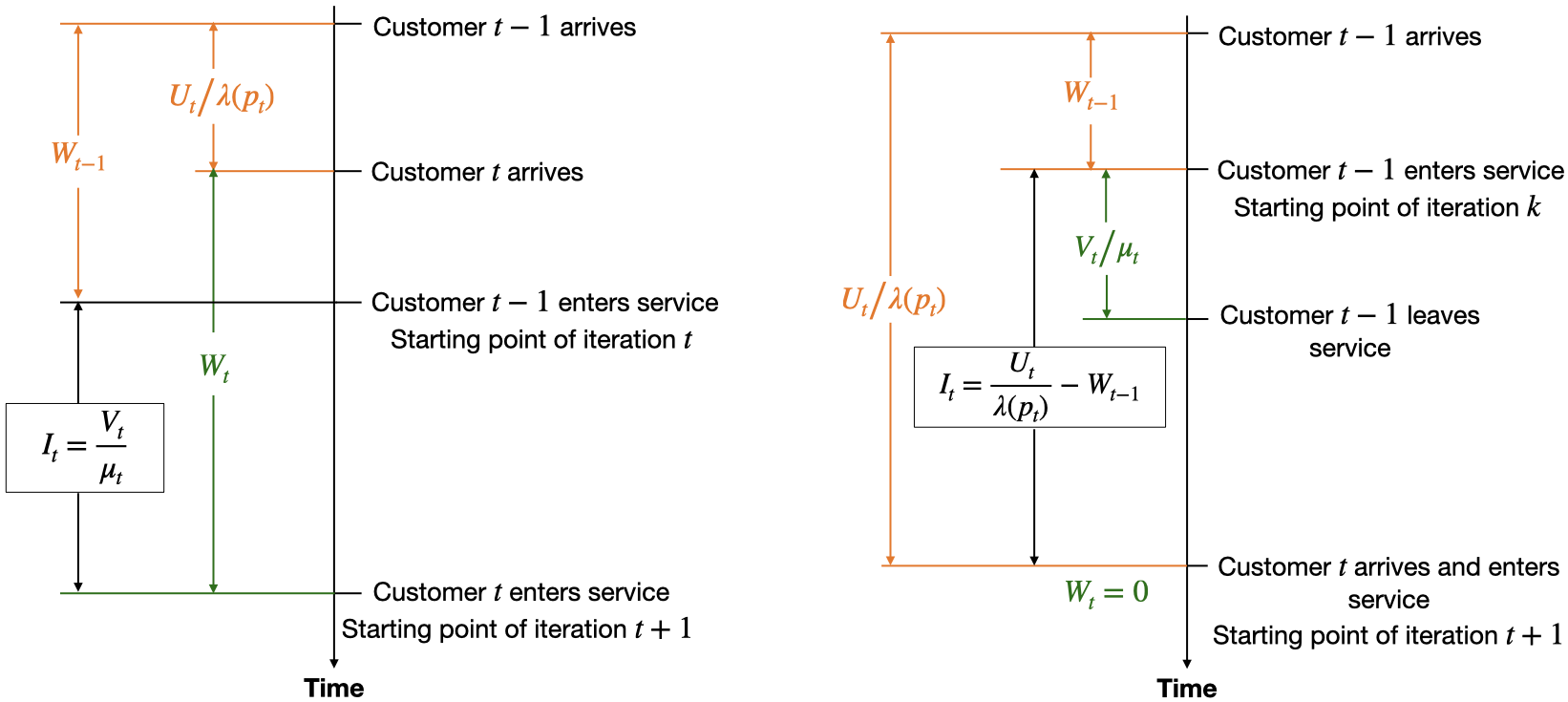
Figure 1: Real-time dynamic of the GI/GI/1 system within a single iteration under SAMCMC. The left panel shows the case where the $t$-th customer arrives before the $(t{-}1)$-th customer leaves, while the right panel shows the opposite case.

Figure 1 illustrates the dynamic of the queueing system at iteration $t$. As the waiting times and observed busy periods are realized when customers enter service, we prescribe that each iteration starts when a customer enters the service and use $I_{t}$ to denote the time interval between the enter-service times of the consequent customer $t{-}1$ and $t$. If the $t$-th customer arrives before the $(t{-}1)$-th customer leaves, then $I_{t}$ corresponds to the service time of customer $t{-}1$, which equals to $I_{t}=\frac{V_{t}}{\mu_{t}}$. If the $t$-th customer arrives after the $(t{-}1)$-th customer leaves, we then should take the idle time where no customer receives service into consideration and find that $I_{t}=\frac{U_{t}}{\lambda(p_{t})}-W_{t-1}$. In both cases, one can verify that

$$I_{t}=W_{t}+\frac{U_{t}}{\lambda(p_{t})}-W_{t-1}.$$

Then, the total time elapsed upon SAMCMC finishes $T$ iterations is $\sum_{t=1}^{T}I_{t}$ and customer $T+1$ enters service then. As a result, the cumulated regret in $T$ iterations is

$$R(T):={\mathbb{E}}\left[\sum\limits_{{t}={2}}^{T+1}(h_{0}(w_{t}+S_{t})-p_{t}+c(\mu_{t})I_{t})-f(\mu^{\star},p^{\star})\sum\limits_{{t}={2}}^{T+1}I_{t}\right],$$ (8)

where $S_{t}:=V_{t}/\mu_{t}$ is the service time of customer $t$. For each $t$, the term $(h_{0}(w_{t}+S_{t})-p_{t}+c(\mu_{t})I_{t})$ can be understood as the cost brought by customer $t$ to the system.

Similar to the regret analysis in (Chen et al., 2023), we decompose the regret $R(T)$ into regret of nonstationarity $R_{1}(T)$ and regret of suboptimality $R_{2}(T)$ as follows

$$R(T) =\underbrace{{\mathbb{E}}\sum\limits_{{t}={2}}^{T+1}\left\{[h_{0}(w_{t}{+}S_{t}){-}p_{t}{+}c(\mu_{t})I_{t}]{-}f(\mu_{t},p_{t})I_{t}\right\}}_{R_{1}(T)}{+}\underbrace{{\mathbb{E}}\sum\limits_{{t}={1}}^{T}(f(\mu_{t},p_{t}){-}f(\mu^{\star},p^{\star}))I_{t}}_{R_{2}(T)},$$

where $R_{1}(T)$ is caused by the transient behavior of the queueing dynamic while $R_{2}(T)$ is caused by the suboptimal choice of control parameters. Applying Theorem 1 that $\|\vartheta_{t}-\vartheta^{*}\|^{2}=O(\eta_{t})$ and Taylor’s expansion of $f(\vartheta_{t})$ around $\vartheta^{*}$, one can check that, if $\eta_{t}=O(t^{-1})$,

$$R_{2}(T)=O\left(\sum_{t=1}^{T}\eta_{t}\right)=O(\log T).$$

Next, we shall deal with the more challenging regret of nonstationary $R_{1}(T)$. The analysis approach for regret of nonstationary developed in Chen et al. (2023) highly depends on the batch-data structure of their algorithm. Roughly speaking, the key step in their analysis is to show that the last observed waiting time in batch $t$ is sufficiently close to $W_{\infty}(\mu_{t},p_{t})$, in expectation, when the batch size is large enough and keeps increasing. In our SAMCMC setting, the batch size is fixed to 1 and thus their analysis approach can not apply. Hopefully, similar to the proof of Lemma 2, by utilizing the continuity of the parameters with respect to the transition kernel, we are able to prove that, the mean difference between $w_{t}$ and $W_{\infty}(\mu_{t},p_{t})$ is still sufficiently small even when the batch size is 1.

Lemma 4.

Let $(\mu_{t},p_{t})$ be the parameter produced by SAMCMC algorithm at iteration $t$. Suppose Assumptions 1 – 3 hold, and the step size is $\eta_{t}=\frac{\gamma}{t}$, where $\gamma$ satisfies the condition $(a)$ as specified in Assumption 4. Then for each $t\geq 1$, it holds that

$${\mathbb{E}}w_{t}-{\mathbb{E}}W_{\infty}(\mu_{t},p_{t})={\mathcal{O}}\left(t^{-1}\right).$$

Proof of Lemma 4.

The proof of Lemma 4 is deferred to Appendix B.3.1. ∎

Remark 8.

Lemma 4 reflects a two-time-scale feature of the joint dynamics of $(\vartheta_{t},x_{t})$ under the SAMCMC algorithm. On the one hand, under Assumption 1, the queueing process $(W_{n},X_{n})$ converges exponentially fast to the stationary distribution for a fixed control parameter $(\mu,p)$ with the exponent uniformly bounded away from 0. On the other hand, the control parameter $\vartheta_{t}$ varies at a much smaller rate proportional to $\eta_{t}\to 0$. As a consequence, one could expect that $x_{t}$ approximately follows the stationary distribution corresponding to $\vartheta_{t}$ in the spirit of the multiscale approximation of stochastic processes (Kurtz, 2005).

Using Lemma 4, we can bound the regret of nonstationary $R_{1}(T)$ by a term of order $O(\log T)$ and thus obtain the total regret bound, as formally stated in Theorem 2 below. Its complete proof is given in Appendix B.3.2.

Theorem 2.

For the cumulative regret given in Eqn.(8), under the step-size choice $\eta_{t}=\frac{\gamma}{t}$ with $\gamma$ satisfying $(a)$ in Assumption 4, we have that

$${\mathbb{E}}R(T)={\mathcal{O}}(\log T).$$

5 Online Statistical Inference

Based on the finite-step convergence rate result in the previous session, we are able to prove a functional central limit theorem for the averaging trajectory of SAMCMC in Section 5.1, which lays down the theoretic foundation for our inference method. In Section 5.2, we describe how to construct confidence intervals using the FCLT result. Finally, we present an efficient computation algorithm in Section 5.3 that produces confidence intervals efficiently from SAMCMC outputs in an online fashion.

5.1 Functional Central Limit Theorem

In order to establish the more general FCLT, additional regularity assumptions are introduced.

Assumption 5.

$($More regularity conditions for FCLT$)$
We additionally assume that

1. There exists a positive definite matrix $G$ and constant $L_{G},\delta_{G}$ such that

   $$\|g(\vartheta)-G(\vartheta-{\vartheta^{\star}})\|\leq L_{G}\cdot\|\vartheta-{\vartheta^{\star}}\|^{2}~{}\text{for any}~{}\|\vartheta-{\vartheta^{\star}}\|\leq\delta_{G}.$$

2. The step size $\eta_{t}$ satisfies both Assumption 4 and the following condition

   $$\eta_{t}\downarrow 0,t\eta_{t}\uparrow\infty,\frac{\eta_{t-1}-\eta_{t}}{\eta_{t-1}}=o(\eta_{t-1}),\sum_{t=1}^{\infty}\eta_{t}=\infty,\sum_{t=1}^{\infty}\eta_{t}^{1.5}<\infty.$$ (9)

Assumption 5 introduces two additional prerequisites. Condition (a) necessitates that the non-linear function $g$ demonstrates local linearity within the vicinity of the root ${\vartheta^{\star}}$. Essentially, this implies that the target gradient $g(\vartheta)$ exhibits a linear behavior in close proximity to ${\vartheta^{\star}}$. Consequently, $g(\vartheta)$ is differentiable at ${\vartheta^{\star}}$, with its derivative represented by the matrix $G$. In other words, $G$ contains the curvature information of the target function $g$ at the root ${\vartheta^{\star}}$. Condition (b) places constraints on the decaying rate of the step size $\eta_{t}$, thereby excluding the use of linearly scaled step sizes, such as $\eta_{t}=\Theta(t^{-1})$, theoretically. In practice, a viable alternative is $\eta_{t}=\gamma\cdot t^{-\alpha}$, where $\alpha\in(2/3,1)$ and $\gamma>0$. A straightforward verification confirms that this chosen step size satisfies both Assumption 4 and the relations given in Eqn. (9).

Before delving into the establishment of the FCLT for $\vartheta_{t}$, it’s crucial to characterize another element: the limiting covariance matrix $S$. Recall that the bi-variate function $U(\vartheta,x)$ serves as the solution to the Poisson equation. To commence, we introduce a covariance matrix that employs this function, which is defined as follows:

$$\mathrm{Var}_{\vartheta}(U({\vartheta^{\star}},x))\equiv P_{\vartheta}U({\vartheta^{\star}},x)U({\vartheta^{\star}},x)^{\top}-\left(P_{\vartheta}U({\vartheta^{\star}},x)\right)\left(P_{\vartheta}U({\vartheta^{\star}},x)\right)^{\top}.$$

Evidently, $\mathrm{Var}_{\vartheta}(U({\vartheta^{\star}},x))$ constitutes the matrix conditional covariance of $U(\vartheta,x)$, with the initiation point being $x$, and a one-step transition conducted along the kernel $P_{\vartheta}$. Consequently, this matrix $\mathrm{Var}_{\vartheta_{t}}(U({\vartheta^{\star}},x_{t-1}))$ depends not only on $x_{t-1}$ but also on $\vartheta_{t}$. It encapsulates the discrepancy that the SAMCMC method may incur during the gradient estimation process $H(x_{t},\vartheta_{t})$. Based on existing assumptions, the following Proposition 3 tells us that the average of $\mathrm{Var}_{\vartheta_{t}}(U({\vartheta^{\star}},x_{t-1}))$ converges in probability towards a covariance matrix which is defined to be $S$, whose proof is deferred to Appendix C.6.

Proposition 3 (Limiting Covariance Matrix).

Under Assumption 3 and 5, and based on Propositions 1, we have that

$$\frac{1}{T}\sum_{t=1}^{T}\mathrm{Var}_{\vartheta_{t}}(U({\vartheta^{\star}},x_{t-1}))\overset{p.}{\to}S.$$

Theorem 3.

With the same condition as in Proposition 3 we have that

$${{\phi}}_{T}(r):=\frac{1}{\sqrt{T}}\sum_{t=1}^{\lfloor Tr\rfloor}(\vartheta_{t}-\vartheta^{\star})\overset{d.}{\to}\mbox{\boldmath$\psi$\unboldmath}(r):=G^{-1}S^{1/2}W(r)$$

within the topology ${\mathcal{D}}([0,1];\left\|{\cdot}\right\|_{\infty})$ which signifies the set of all càdlàg functions defined on $[0,1]$ equipped with the maximum norm $\left\|{\cdot}\right\|_{\infty}$. Here $G$ is the local linearity matrix defined in Assumption 5, $S$ is the limiting covariance matrix given in Proposition 3 and $W(\cdot)$ is a standard $d_{\vartheta}$-dimension Brownian motion.

Theorem 3 shows both the cadlag constant function ${\phi}_{t}$ weakly converges to the rescaled Brownian motion $G^{-1}S^{1/2}W$. The scale $G^{-1}S^{1/2}$ is the nuisance parameter that involves both the local linearity coefficient $G$ and the covariance matrix $S$.

Remark 9.

The proof of Theorem 3 follows the approach outlined in Li et al. (2023a). This proof method uses a so-called Martingale-residual-coboundary decomposition. By applying this approach, the centered gradient $H(x_{t},\vartheta_{t})-g(\vartheta_{t})$ is partitioned into three distinct terms: a martingale term, a residual term, and a coboundary term. Leveraging the convergence rate established in Theorem 1, we can show that both the residual and coboundary terms exhibit higher-order convergence compared to the martingale term. This property facilitates the decomposition of the partial-sum process ${{\phi}}_{T}(r)$ into two main components: a partial-sum process of martingale differences, and an additional higher-order reminder process. Classic results imply the former partial-sum process weakly converges to the scaled Brownian motion $G^{-1}S^{1/2}W(r)$. The subsequent step involves establishing the convergence of the reminder process towards a zero process within the framework of the uniform topology. The detailed proof of this theorem can be found in Appendix C.1.

By invoking the continuous mapping theorem, we are able to derive Corollary 1. This corollary helps us to restore the asymptotic normality result documented in Liang (2010) simply by selecting $h(\phi)$ as $\phi(1)$, resulting in Corollary 2.

Corollary 1.

Under the same condition in Theorem 3, for any continuous functional $h:D\to{\mathbb{R}}^{d}$, it follows that as $T\to\infty$,

$$h({{\phi}}_{T})\overset{d}{\to}h(\psi).$$

Corollary 2.

Under the same condition in Theorem 3, setting $h(\phi):\phi\mapsto\phi(1)$,

$${{\phi}}_{T}(1)\overset{d}{\to}\psi(1),~{}i.e.,~{}\frac{1}{\sqrt{T}}\sum_{t=1}^{T}(\vartheta_{t}-{\vartheta^{\star}})\overset{d}{\to}{\mathcal{N}}(0,G^{-1}SG^{-\top}).$$

5.2 Construction of Confidence Intervals

Conventional wisdom in developing online inference methods entails estimating the asymptotic variance matrix, $G^{-1}SG^{-\top}$ and plugging it into the asymptotic normality in Corollary 2 (Chen et al., 2020, 2021; Li et al., 2022). However, this endeavor is particularly formidable within our context, given its intricate connection to both the local linearity coefficient $G$ and the solution $U(\vartheta,\cdot)$ to the Poisson equation. The task of estimating this matrix remains an open challenge in the context of a SA procedure using Markovian data. On another note, even the estimation of $G$ and $S$ is attainable within our framework; the computation involving the matrix inversion $G^{-1}$ and the multiplication $G^{-1}S$, however, incurs a computational cost of up to $O(d^{3})$, with the added need for $O(d^{2})$ memory to store intermediate outcomes. This conundrum leads us to explore the existence of an efficient online inference method that bypasses the need to estimate any matrix spanning between $S$ and $G$ while maintaining a computational expense of up to $O(d)$ and a memory requirement of up to $O(d)$.

Fortunately, the FCLT offers a positive response to this query. Corollary 1 brings forth a pivotal insight: when $h$ exhibits scale-invariance - such that $h(O{\phi})=h({\phi})$ for any non-singular matrix $O\in\mathbb{R}^{d\times d}$ and any cadlag process ${\phi}$ - the outcome is that

$$h({\phi}_{T})\overset{d}{\to}h(\psi)=h(G^{-1}S^{1/2}W)=h(W).$$

This implies that the distributional convergence of $h({\phi}_{T})$ is towards a functional reliant on the standard Brownian motion, $h(W)$. Scrutinizing further, it’s apparent that $h({\phi}_{T})$ represents a pivotal entity, solely entwined with collected data and the unknown root ${\vartheta^{\star}}$. Conversely, $h(W)$ boasts a known distribution, rendering its quantiles computable through simulation. This dynamic facilitates the construction of asymptotic confidence intervals. Therefore, FCLT underpins the foundational rationale of our statistical inference approach. We make this point more precise in the following proposition.

Proposition 4.

Under the same condition in Theorem 3, given any unit vector $v\in{\mathbb{R}}^{d}$ and a continuous scale-invariant functional $h:D\to{\mathbb{R}}$, it follows that when $T\to\infty$,

$${\mathbb{P}}\left(v^{\top}{{\vartheta^{\star}}}\in{\mathcal{C}}(\alpha,h,\phi_{T})\right)\to 1-\alpha,$$

where ${\mathcal{C}}(\alpha,h,\phi_{T})$ is the $\alpha$-level confidence set defined by

$${\mathcal{C}}(\alpha,h,\phi_{T}):=\left\{v^{\top}{\vartheta^{\star}}\in{\mathbb{R}}:|h(v^{\top}{\phi}_{T})|\leq q_{\alpha,h}\right\}$$ (10)

and $q_{\alpha,h}$ is the critical value defined by

$$q_{\alpha,h}=\sup\{q:{\mathbb{P}}(|h(W)|\geq q)\leq\alpha\}.$$ (11)

The feasibility of the aforementioned construction of confidence intervals hinges on the presence of an appropriate scale-invariant functional, denoted as $h(\cdot)$. A typical choice in the literature is given in the following functional (Li et al., 2023a, b, 2022; Lee et al., 2022a, b)

$$h(\chi)=\frac{\chi(1)}{\sqrt{\int_{0}^{1}(\chi(r)-r\chi(1))^{2}dr}}.$$ (12)

One can show that this $h$, as a one-dimensional functional, is not only scale-invariant so that $h(a\chi)=a\cdot h(\chi)$ for any non-negative $a\geq 0$ but also symmetric in the sense that $h(-\chi)=-h(\chi)$ for any cadlag process $\chi$. With this specific functional $h$, this confidence interval (10) has a more concrete form as shown in the following corollary.

Corollary 3.

Under the same condition in Theorem 3, then as $T\to\infty$,

$${\mathbb{P}}\left(v^{\top}{\vartheta^{\star}}\in\left[v^{\top}\bar{\vartheta}_{T}-q_{\alpha,h}\bar{\sigma}_{T},v^{\top}\bar{\vartheta}_{T}+q_{\alpha,h}\bar{\sigma}_{T}\right]\right)\to 1-\alpha,$$ (13)

where $\bar{\vartheta}_{T}=\frac{1}{T}\sum_{i=1}^{T}\vartheta_{i}$ is the average of the first $T$ iterates and

$$\bar{\sigma}_{T}=\frac{1}{T}\sqrt{\sum_{i=1}^{T}i^{2}|v^{\top}(\bar{\vartheta}_{i}-\bar{\vartheta}_{T})|^{2}}$$

is an approximation of the denominator $\sqrt{\int_{0}^{1}(v^{\top}{\phi}_{T}(r)-rv^{\top}{\phi}_{T}(1))^{2}dr}$.

Prior research has adopted two distinct strategies to compute the critical values $q_{\alpha,h}$ for $h(W)$: stochastic simulation (Kiefer et al., 2000) and density approximation (Abadir and Paruolo, 1997). In our study, we employ the former approach and present our computed estimates in Table 1 for convenient reference.

Remark 10.

By the definition of $\bar{\vartheta}_{T}$, when $r=\frac{i}{T}$ for any $i\in[T]$, we have $v^{\top}{\phi}_{T}(r)=\frac{i}{\sqrt{T}}v^{\top}(\bar{\vartheta}_{i}-{\vartheta^{\star}})$ and then

$$v^{\top}({\phi}_{T}(r)-r{\phi}_{T}(1))=\frac{i}{\sqrt{T}}v^{\top}(\bar{\vartheta}_{i}-\bar{\vartheta}_{T}),$$

which remains independent of the unknown root ${\vartheta^{\star}}$. This observation motivates us to use the rectangle rule to compute the integral $\int_{0}^{1}({\phi}_{T}(r)-r{\phi}_{T}(1))^{2}dr$, i.e.,

$$\int_{0}^{1}(v^{\top}{\phi}_{T}(r)-rv^{\top}{\phi}_{T}(1))^{2}dr \approx\frac{1}{T}\sum_{i=1}^{T}\left(v^{\top}{\phi}_{T}\left(\frac{i}{T}\right)-\frac{i}{T}v^{\top}{\phi}_{T}\left(1\right)\right)^{2}$$

$$=\frac{1}{T^{2}}\sum_{i=1}^{T}i^{2}(v^{\top}\bar{\vartheta}_{i}-v^{\top}\bar{\vartheta}_{T})^{2}=:\bar{\sigma}_{T}^{2}.$$

Numerical evidence in (Li et al., 2023a) confirms that this approximation exhibits high accuracy in practice and adequately delivers satisfactory performance.

As illustrated by the concrete example, the scale-invariant property is closely linked to the utilization of the entire trajectory iterates $\{\vartheta_{t}\}_{t\in[T]}$. This rationale underscores the necessity for a stronger FCLT outcome beyond the asymptotic normality of trajectory averages.

$1-\alpha$	$1\%$	$2.5\%$	$5\%$	$10\%$	$50\%$	$90\%$	$95\%$	$97.5\%$	$99\%$
$q_{\alpha,h}$	-8.628	-6.758	-5.316	-3.873	0.000	3.873	5.316	6.758	8.628

Table 1: Asymptotic critic values $q_{\alpha,h}$ defined in (11). They are computed via simulations. In particular, the Brownian motion $W$ is approximated by normalized sums of i.i.d. ${\mathcal{N}}(0,1)$ pseudo-random deviates using 1,000 steps and 50,000 replications.

5.3 An Efficient Online Computation Algorithm

The remaining issue is how to compute the confidence interval (13) efficiently online. Actually, this work has already been done in previous works (Lee et al., 2022a; Li et al., 2022, 2023a). For completeness, we formally introduce this online computation algorithm, analyze its computation and memory cost, and present its extensions.

According to Corollary 3, we only need to identify an online incremental update for both $\bar{\vartheta}_{t}$ and $\bar{\sigma}_{t}$. On one hand, the moving average $\bar{\vartheta}_{t}$ can be naturally computed online due to the relation $\bar{\vartheta}_{t+1}=\frac{T}{t+1}\bar{\vartheta}_{t}+\frac{1}{t+1}\vartheta_{t+1}$. On the other hand, we note that $\sum_{i=1}^{t}i^{2}|v^{\top}(\bar{\vartheta}_{i}-\bar{\vartheta}_{t})|^{2}$, as the key component in $\bar{\sigma}_{t}^{2}$, can be decomposed into the sum of three terms as follows

$$\sum_{i=1}^{t}i^{2}|v^{\top}(\bar{\vartheta}_{i}-\bar{\vartheta}_{t})|^{2} =\sum_{i=1}^{t}i^{2}\left((v^{\top}\bar{\vartheta}_{i})^{2}-2v^{\top}\bar{\vartheta}_{i}v^{\top}\bar{\vartheta}_{t}+(v^{\top}\bar{\vartheta}_{t})^{2}\right)$$

$$=\sum_{i=1}^{t}i^{2}((v^{\top}\bar{\vartheta}_{i})^{2}-2\sum_{i=1}^{t}i^{2}v^{\top}\bar{\vartheta}_{i}v^{\top}\bar{\vartheta}_{t}+\sum_{i=1}^{t}i^{2}(v^{\top}\bar{\vartheta}_{t})^{2}$$

$$=O_{t,1}-2O_{t,2}\cdot(v^{\top}\bar{\vartheta}_{t})+O_{t,3}\cdot(v^{\top}\bar{\vartheta}_{t})^{2},$$ (14)

where we define the following notation for simplicity

$$O_{t,1}=\sum_{i=1}^{t}i^{2}((v^{\top}\bar{\vartheta}_{i})^{2},~{}O_{t,2}=\sum_{i=1}^{t}i^{2}v^{\top}\bar{\vartheta}_{i},~{}\text{and}~{}O_{t,3}=\sum_{i=1}^{t}i^{2}.$$

Once $v^{\top}\bar{\vartheta}_{t}$ is obtained, $O_{t,j}$ can be updated to $O_{t+1,j}$ using only $O(1)$ computation for any $j\in[3]$. Indeed, it directly follows from the fact that

$$O_{t+1,1} =O_{t,1}+(t+1)^{2}(v^{\top}\bar{\vartheta}_{t+1})^{2}$$ (15a)

$$O_{t+1,2} =O_{t,2}+(t+1)^{2}(v^{\top}\bar{\vartheta}_{t+1})$$ (15b)

$$O_{t+1,3} =O_{t,3}+(t+1)^{2}.$$ (15c)

As a result, updating $\bar{\sigma}_{t}$ to $\bar{\sigma}_{t+1}$ requires only $O(d)$ computations which happen in the evaluation of the inner product $v^{\top}\bar{\vartheta}_{t}$. Because we only need to maintain three one-dimensional sequences $\{O_{t,j}\}_{j\in[3]}$ and the average $\bar{\sigma}_{t}$, the memory cost is also $O(d)$, which scales linearly with the dimension $d$.

We summarize this online computation algorithm in Algorithm 2.

  Input: $\{\eta_{t}\}$, linear coefficient $v$, initial state $x_{0}$ and parameter $\vartheta_{0}$.   for Iteration $t\geq 1$ do      Sample $x_{t}$ from the transition probability distribution $P_{\vartheta_{t}}(x_{t-1},\cdot)$.      Update $\vartheta_{t+1}\leftarrow\Pi_{\Theta}(\vartheta_{t}-\eta_{k}H(\vartheta_{t},x_{t}))$, where $\Pi_{\Theta}$ is the projection operator.      Compute $\bar{\vartheta}_{t+1}=\frac{t}{t+1}\bar{\vartheta}_{t}+\frac{1}{t+1}\vartheta_{t+1}$.      Compute the value of the inner product $v^{\top}\bar{\vartheta}_{t+1}$.      Perform the updates in (15) and obtain $\{O_{t+1,j}\}_{j\in[3]}$.      Compute $\bar{\sigma}_{t+1}=\frac{1}{t+1}\sqrt{O_{t+1,1}-2O_{t+1,2}\cdot(v^{\top}\bar{\vartheta}_{t+1})+O_{t+1,3}\cdot(v^{\top}\bar{\vartheta}_{t+1})^{2}}$.      Output the current confidence interval $\left[v^{\top}\bar{\vartheta}_{t+1}-q_{\alpha,h}\bar{\sigma}_{t+1},v^{\top}\bar{\vartheta}_{t+1}+q_{\alpha,h}\bar{\sigma}_{t+1}\right]$.   end for

Algorithm 2 SAMCMC with Online Confidence Intervals

Remark 11.

In a related study, Li et al. (2023a) introduced a family of scale-invariant functionals, expressed as $h_{m}({\phi})=\frac{\chi(1)}{\sqrt[m]{\int_{0}^{1}(\chi(r)-r\chi(1))^{m}dr}}$, which encompasses the formulation in (12) as a special case. This framework provides a structured approach for different values of $m$. For even values of $m$, the denominator $\int_{0}^{1}(\chi(r)-r\chi(1))^{m}$ can be decomposed similarly to (5.3). Consequently, the computational complexity and memory requirements at each iteration remain at $O(d)$ for online statistical inference. For the sake of simplicity and illustrative purposes, we focus on the case in (12).

6 Numerical Experiments

To test the actual performance of the SAMCMC algorithm and our online inference method, we conduct a series of numerical experiments on steady-state optimization of GI/GI/1 queue. In particular, to confirm the practical effectiveness of our online learning method, we conduct numerical experiments to visualize the algorithm convergence, and benchmark the outcomes with known exact optimal solutions, estimate the true regret, and compare it to the theoretical upper bounds. We also verify the asymptotic normality of SAMCMC and test the consistency of our online inference method in Section 6.4.

6.1 Experiment Setting

We implement SAMCMC on three GI/GI/1 models with different inter-arrival and service time distributions as considered in Chen et al. (2023). In all settings , we use a logistic demand function $\lambda(\cdot)$ in the form of

$$\lambda(p)=M\cdot\frac{\exp(a-p)}{1+\exp(a-p)}.$$ (16)

where $M$ is interpreted as the market size. In the following experiments, we set $M=10$, $a=4.1$ and the coefficient of holding cost $h_{0}=1$ in the objective function (3). Below, we specify the setting details of the three queueing models one by one.

M/M/1 Queue

The first example is the fundamental M/M/1 queue with Poisson arrivals and exponential service times. Following Chen et al. (2023), we consider a quadratic cost function for service rate $\mu$

$$c(\mu)=\frac{c_{0}}{2}\cdot\mu^{2}.$$ (17)

In this case, the objective function (3) has a closed-form expression as

$$\min_{(\mu,p)\in\mathcal{B}}\left\{h_{0}\frac{\lambda(p)}{\mu-\lambda(p)}+\frac{c_{0}}{2}\mu^{2}-p\lambda(p)\right\},$$

from which the exact values of the optimal solutions $(\mu^{\star},p^{\star})$ and the corresponding objective value $f(\mu^{\star},p^{\star})$ can be obtained via numerical methods. We set $c_{0}=1$ and $\mathcal{B}=[3.5,10]\times[6.56,15]$, which results the optimal solution $(\mu^{\star},p^{\star})=(4.0234,7.103)$.

M/GI/1 Queue

The famous Pollaczek-Khinchine (PK) formula provides a closed-form expression for the steady-state average queue length the for M/GI/1 model:

$$\mathbb{E}[Q_{\infty}(\mu,p)]=\rho+\frac{\rho^{2}}{1-\rho}\frac{1+c_{s}^{2}}{2},$$ (18)

where $\rho=\frac{\lambda(p)}{\mu}$ is the traffic intensity under the parameter $(p,\mu)$ and $c_{s}^{2}=\mathrm{Var}(V)/[\mathbb{E}V]^{2}$ is the squared coefficient of variation (SCV) for the service time random variable $V$.

To introduce an additional degree of flexibility for $c_{s}$, we adopt the Erlang-$k$ distribution for the service-time distribution whose SCV equals $1/k$. In the special case when $k=1$, the Erlang-1 distribution is reduced to the Poisson distribution, and the corresponding M/GI/1 queue is reduced to an M/M/1 queue. For the M/GI/1 model, we consider a linear staffing cost function

$$c(\mu)=c_{0}\cdot\mu.$$ (19)

In our experiments, we fix $c_{0}=1$ and $\mathcal{B}=[3.5,7]\times[6.5,10]$ but vary $k$ to make $c_{s}$ range from $0.1$ to $3$ equidistantly, with a total of 200 different $c_{s}$’s. The optimal solutions $(\mu^{\star},p^{\star})$ and traffic intensity $\rho^{*}\equiv\lambda(p^{*})/\mu^{*}$ corresponding to different values of $c_{s}$, together with the last-iterate performance of the SAMCMC algorithm, are reported in Figure 2. Noting that M/M/1 corresponds to the case where $c_{s}=1$, we also examine two specific scenarios where $c_{s}\in\{0.5,1.5\}$ for further case study.

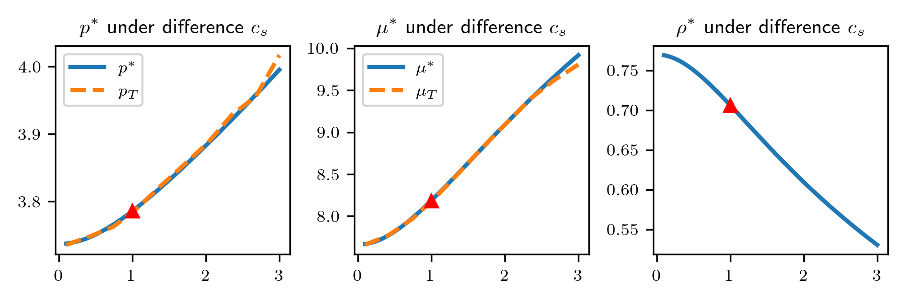
Figure 2: Optimal controls of M/GI/1 queue with different values of $c_{s}$. The true values of optimal $\mu^{\star}$, $p^{\star}$, and $\rho^{*}$ are depicted by the solid blue curves, where the $x$-axis represents the value of $c_{s}$. The dashed orange curves report the averages of the final output of SAMCMC with $T=10^{5}$ iterations in 100 repetitions. The red triangles mark the optimal values of the M/M/1 queue when $c_{s}=1$.

GI/M/1 Queue

For the queueing model with general inter-arrival time distributions, we consider an $E_{2}$/M/1 queue – a system characterized by Erlang-2 interarrival times and exponential service times. The main purpose for us to use this setting is that efficient numerical methods are available for computing the true value of the optimal $(\mu^{*},p^{*})$ and objective function, employing the matrix geometric approach.

In this experiment, we use linear staffing cost with $c_{0}=1$ and $\mathcal{B}=[3.5,7]\times[6.5,10]$, which yields the optimal decision $(\mu^{\star},p^{\star})=(3.762,7.935)$.

Benchmark algorithm

We select a simplified version of GOLiQ proposed in Chen et al. (2023) as the benchmark algorithm as it provides explicit guidance on the choice of batch size and other algorithm parameters. GOLiQ differs from SAMCMC in estimating the gradient $\nabla f(\vartheta_{t})$ using an increasing number (or batch size) of samples collected under the current policy parameterized by $\vartheta_{t}$. Following the guidance in Chen et al. (2023), we use different choices of batch size in the form of $1+b_{c}\log t$ for the $t$-th estimate of the gradient with $b_{c}\in\{1,5,10,20\}$ to test the effect of batch sizes. Our SAMCMC algorithm corresponds to the case when $b_{c}=0$.

We then implement SAMCMC and the benchmark GOLiQ on all three queuing settings and run 200 rounds of simulation. In all experiments, the initial value $(\mu_{1},p_{1})=(3.5,8)$. The step size is fixed with $\eta_{t}^{p}=\frac{1.25}{t}$ for the update of $p$ and $\eta_{t}^{\mu}=\frac{12.5}{t}$ for the update of $\mu$. Next, we compare their performance in terms of sample complexity and cumulated regret and test the robustness of SAMCMC with respect to the choice of step size $\eta_{t}$.

6.2 Convergence and Regret Results

The numerical results of SAMCMC and GOLiQ with different choices of $b_{c}$ are reported in Figures 3 to 5 corresponding to different queueing model settings. In each figure, the top two panels report the averaged trajectories of the control parameter $p_{t}$ and $\mu_{t}$, respectively, while the left-bottom panel reports the average $L_{2}$ difference between $\vartheta_{t}$ and $\vartheta^{*}$ and the right-bottom one reports the average cumulated regret. The $x$-axes denote the number of data samples, or equivalently, the number of customers served, in all panels.

Our first observation is that increasing batch size does not help either in improving the convergence rate or in reducing cumulated regret in all the queueing models. This encores our theoretic result that gradient estimation with a single data point is adequate for controlling transient bias and guaranteeing algorithm convergence. The difference between SAMCMC and GOLiQ is more significant when $b_{c}\geq 5$, which can be attributed to an overemphasis on gradient quantity at the expense of the optimization process itself, as an excessive number of samples are allocated to refining gradient estimates rather than advancing the optimization trajectory. When $b_{c}=1$, the batch size $1+b_{c}\log(t)$ is close to $1$ for small $t$, as a consequence, we see that the two curves corresponding to SAMCMC and GOLiQ with $b_{c}=1$ are similar in the early iterations but gradually deviate from each other in the later iterations.

Comparing Figures 4, 3, and 5 corresponding to $M/GI/1$ models with $c_{s}=0.5,1$ and $1.5$, respectively, we find that the improvement of SAMCMC over GOLiQ seems more significant when there is more variability in the system dynamics, i.e. with larger value of $c_{s}$. A more rigorous analysis of this phenomenon is left for future study.

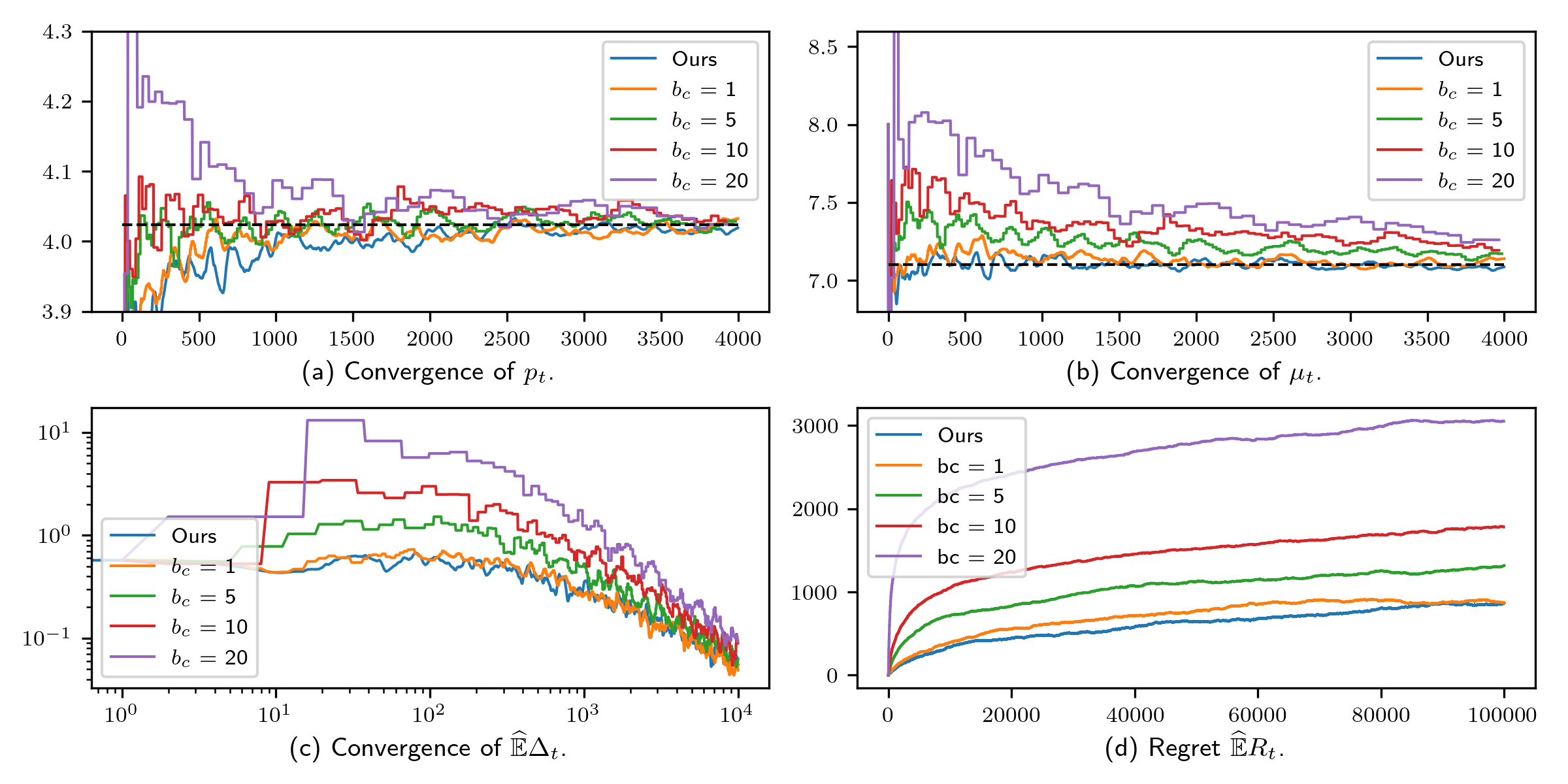
Figure 3: Convergence and regret in the M/M/1 setting over 200 repetitions.

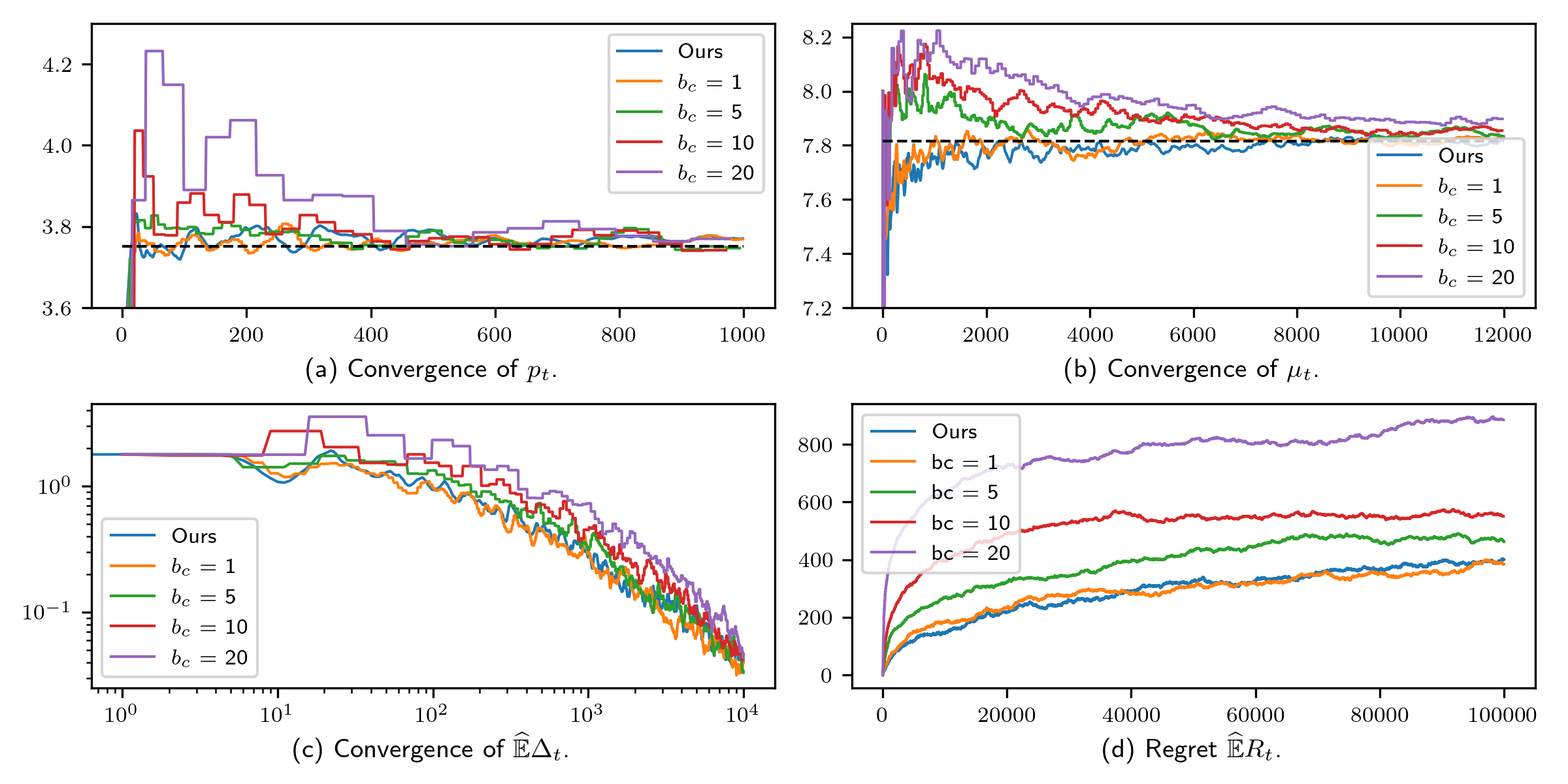
Figure 4: Convergence and regret in the M/GI/1 setting with $c_{s}=0.5$ over 200 repetitions.

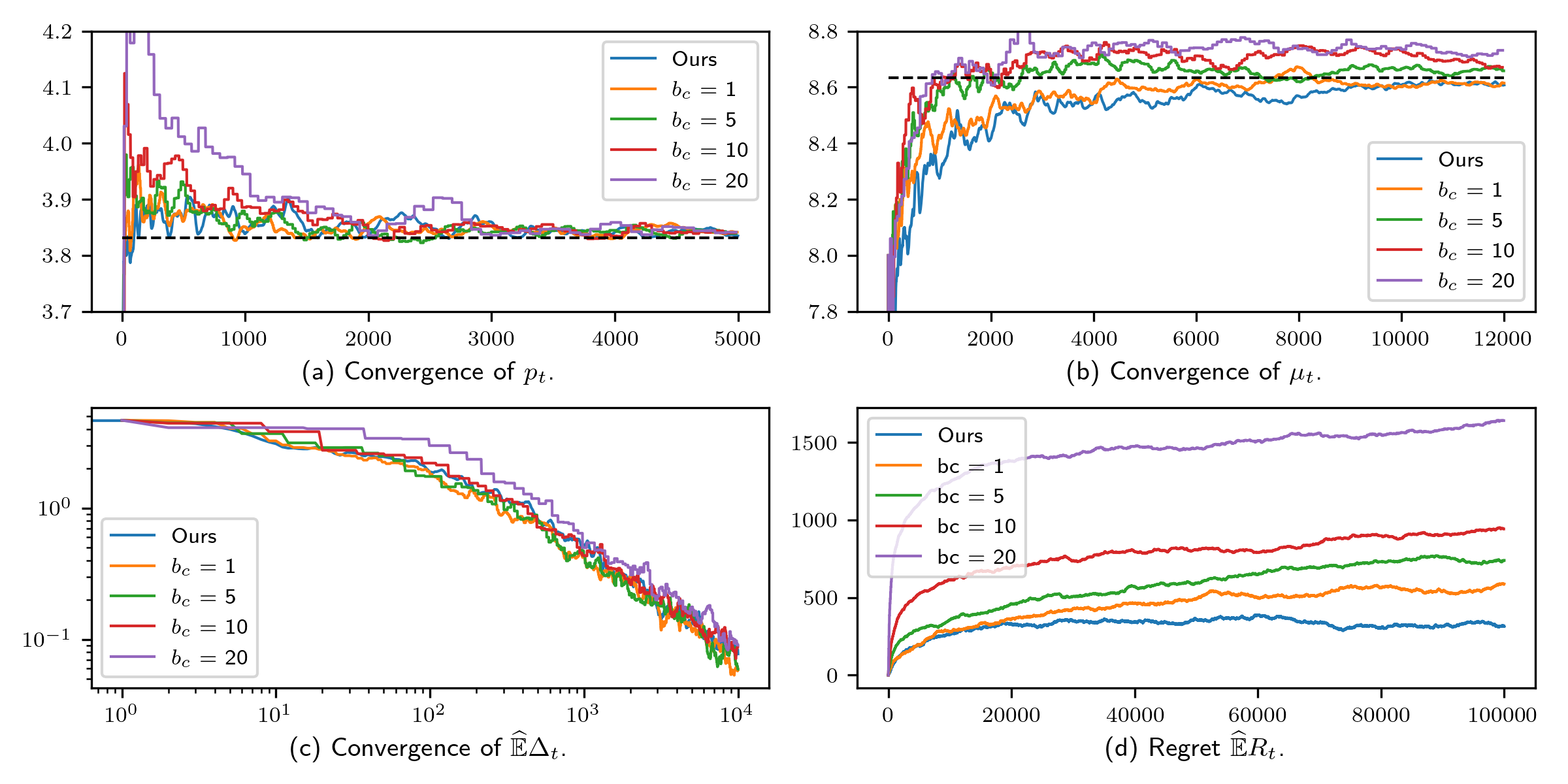
Figure 5: Convergence and regret in the M/GI/1 setting with $c_{s}=1.5$ over 200 repetitions.

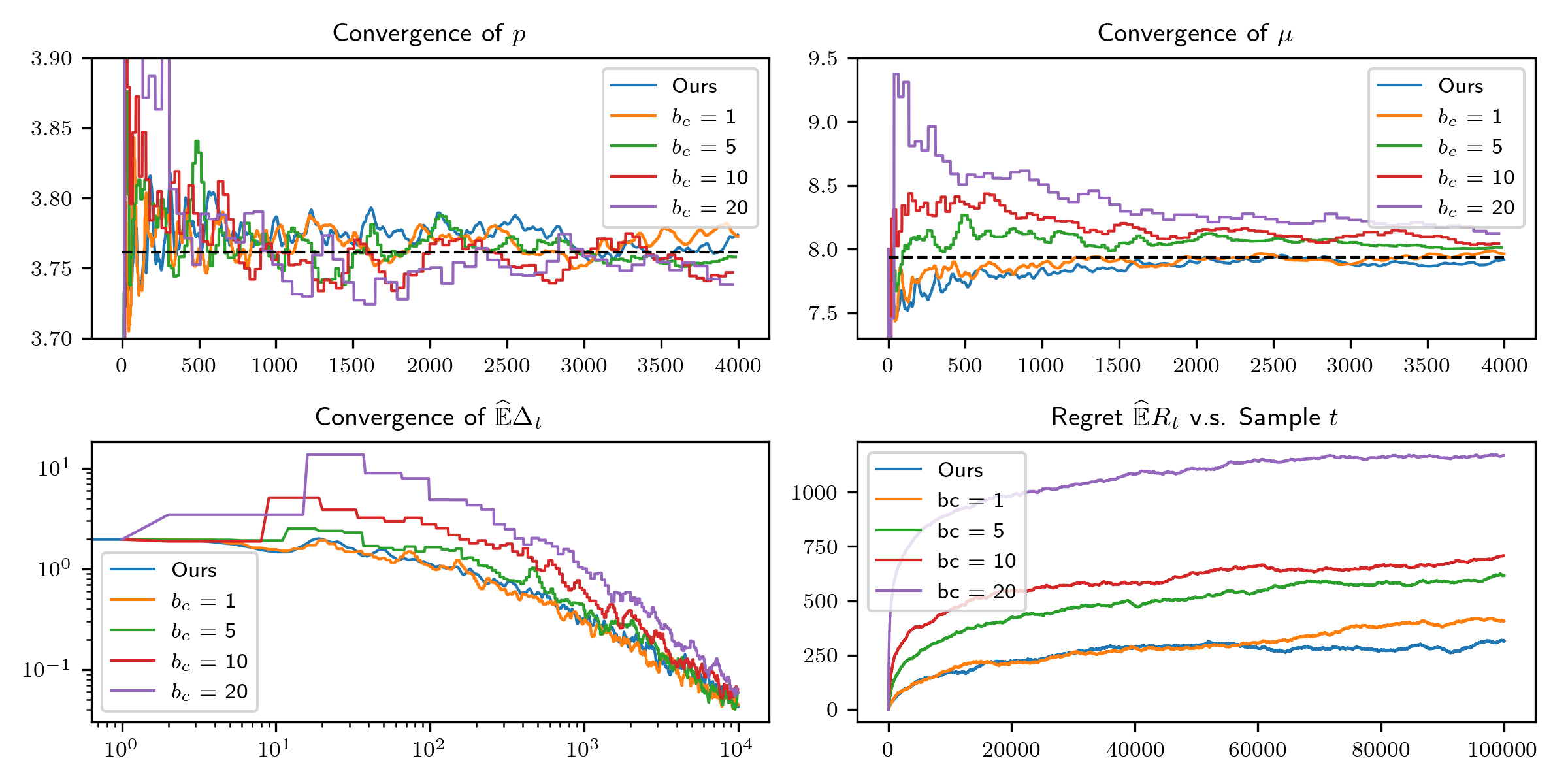
Figure 6: Convergence and regret in the GI/M/1 setting over 200 repetitions.

6.3 Robustness Check on the Step Sizes

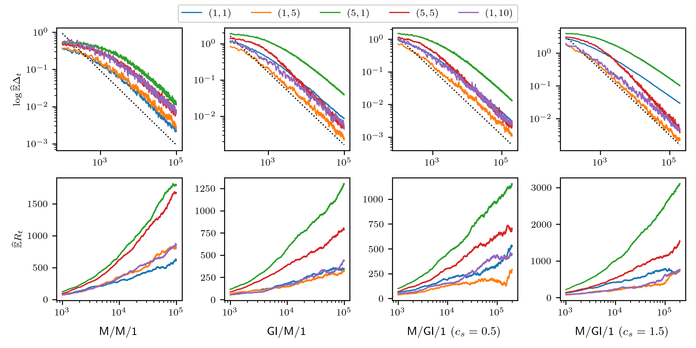
Figure 7: Convergence and regrets with different step size parameters $(c_{p},c_{\mu})$ in the four settings over 200 repetitions.

While our theory uses the same step size $\eta_{t}$, we experiment with different step sizes for different coordinates. From the theoretic aspect, this discrepancy does not pose a critical problem. An effective amendment is to substitute the standard Euclidean norm with a weighted one. Specifically, for any set of positive weights denoted as $w_{i}>0$ for $i\in[d]$, if we intend to implement a separate step size $\eta_{t,i}=w_{i}\eta_{t,0}$ to update the $i$-th coordinate, we could replace the inner product $\langle x,y\rangle=\sum_{i=1}^{d}x_{i}y_{i}$ with a weighted counterpart $\langle x,y\rangle_{w}=\sum_{i=1}^{d}x_{i}y_{i}w_{i}$ in all our theoretical assumptions. This adaptation retains its efficacy as long as all the step sizes $\{\eta_{t,i}\}_{i\in[d]}$ approach zero uniformly at the same rate. Under these new assumptions, the fundamental tenets of our theoretical framework remain preserved without changing the proof too much.

In addition to the above amendment to the convergence theory, we next test the robustness of the choice of step sizes numerically. Allowing the flexibility of employing distinct yet proportionate step sizes for different coordinates, we implement SAMCMC with a set of different step sizes in the form of $\eta_{t}^{p}=\frac{c_{p}}{1+t}$ for updating $p$ and $\eta_{t}^{\mu}=\frac{c_{\mu}}{1+t}$ for $\mu$ updates with $(c_{p},c_{\mu})\in\{(1,1),(1,5),(5,1),(5,5),(1,10)\}$.

In the top panel of Figure 7, we plot the logarithmic of the resulting $L_{2}$ difference versus the logarithmic of the number of data samples. We see that all the curves can be well fitted by some 45-degree line as depicted in the graphs, indicating that the $O(t^{-1})$ convergence rate holds in all queueing settings with different choices of step size. In the bottom panel of Figure 7, we plot the cumulated regret versus the logarithmic of the number of data samples. Consistent with the theoretic $O(log(t))$ regret bounds, in all settings, the curve of regret becomes close to a straight line, although with different slopes, in the later iterations. To this light, our numerical results illustrate the robustness of SAMCMC with respect to the choice of step sizes in both dimensions.

Another interesting observation is that step size combinations $(1,5)$ and $(1,10)$ perform slightly better than the coordinately equal step size $(1,1)$. One possible explanation is that the objective function, along the dimension of staffing level $\mu$, is flatter around the optimal solution, compared to that along the dimension of price $p$ (see figure 6 of Chen et al. (2023)). As a consequence, applying a larger step size to $\mu$ could help improve algorithm convergence.

6.4 Numerical Performance of Online Inference Method

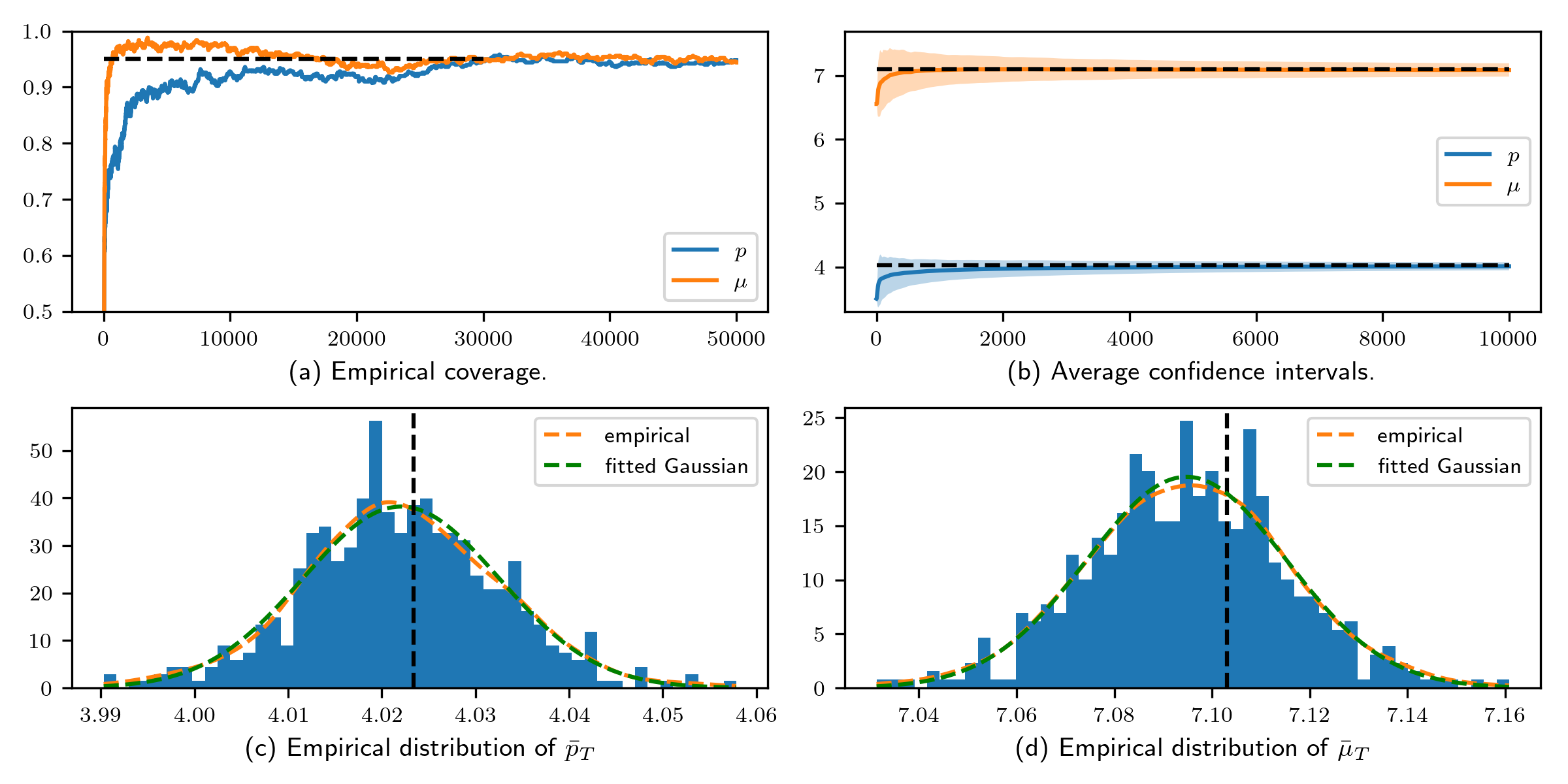
Figure 8: Online inference for M/M/1 queues over 500 repetitions with $\alpha=0.99$.

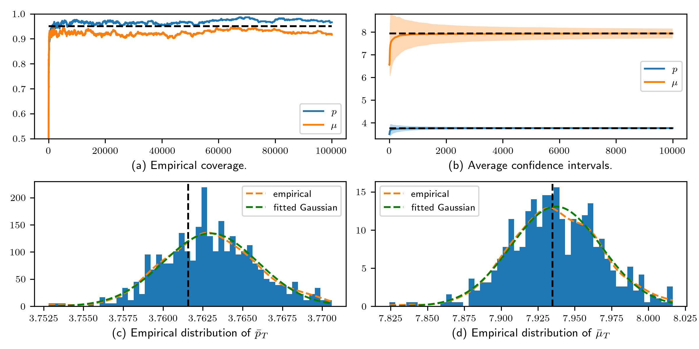
Figure 9: Online inference for GI/M/1 queues over 500 repetitions with $\alpha=0.99$.

We retain the same three experimental setups introduced in Section 6.1. To ensure consistency with our theoretical framework, we adopt polynomial step sizes across all experiments detailed in this section. Specifically, we employ $\eta_{t,p}=\frac{c_{p}}{(1+t)^{\alpha}}$ for updating the parameter $p$, and $\eta_{t,\mu}=\frac{c_{\mu}}{(1+t)^{\alpha}}$ for updating $\mu$, where we set $(c_{p},c_{\mu})=(1,20)$ and $\alpha=0.99$. To provide a comprehensive overview, we also furnish results for the same step sizes with $\alpha=1$ in the appendix. It is worth noting that similar performance trends have been observed under these conditions.

In each of Figures 8 to 11 below, we report (a) the empirical coverage rate across 500 repetitions and (b) visualization of averaged confidence intervals. To better depict the actual distribution of the averaged estimators $\bar{p}_{T}$ and $\bar{\mu}_{T}$, we report their histograms across the 500 repeated experiments along with the fitted Gaussian distributions in panels (c) and (d), respectively. We also display the distributions fitted using Gaussian kernel density methods, denoted as “empirical”, as a nonparametric alternative to illustrate the empirical distribution.

Consistent with Corollary 3, the empirical coverage rate progressively increases as the iterations advance and the volume of received samples grows, as illustrated in panels (a). In addition, the empirical coverage rates converge around the intended $95\%$ coverage rate in all settings. Furthermore, in panel (b), we see that the averaged confidence intervals showcase a consistent tendency to cover the true parameters while gradually dwindling its confidence interval lengths.

The histograms of $\bar{p}_{T}$ or $\bar{\mu}_{T}$ are well approximated by the fitted Gaussian distributions, aligning with the expectations laid out in Corollary 2. It’s important to note that the perceived deviation of the true parameter (denoted by black dotted straight lines) from the centers of both empirical and fitted Gaussian distributions is misleading, primarily due to the diminutive scale of the $x$-axis. For instance, in Figure 8, the mean of the estimated Gaussian distributions deviates from the true parameter by no more than 0.004 – an exceedingly minimal error.

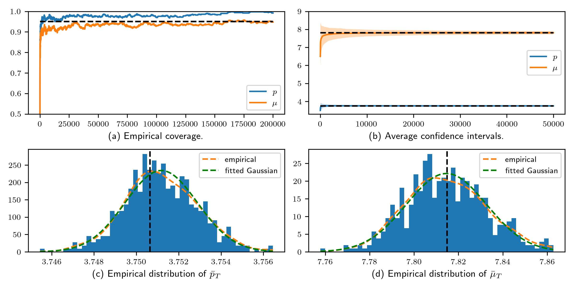
Figure 10: Online inference for M/GI/1 queues with $c_{s}=0.5$ over 500 repetitions with $\alpha=0.99$.

Figure 11: Online inference for M/GI/1 queues with $c_{s}=1.5$ over 500 repetitions with $\alpha=0.99$.

7 Concluding Remarks

In this paper, we propose a stochastic approximation MCMC (SAMCMC) algorithm for steady-state optimization of queueing systems and develop a novel online inference method to quantify the uncertainty of the SAMCMC output. For theoretic verification of the efficiency of our proposed algorithms, we establish both a non-asymptotic convergence rate and regret bound for the final output of SAMCMC and derive the functional central limit theory for the averaging trajectory of the SAMCMC output sequence, which is of independent research interest. Our theoretical results are built on Propositions 1 to 2, which are commonly made as the assumptions in the stochastic approximation literature. Thus, if similar conditions are satisfied, we could apply our convergence results and inference methods to a general SAMCMC setting beyond the current queueing system. To the best of our knowledge, we are the first to explore the SAMCMC algorithm along with the online statistical inference for the GI/GI/1 queueing optimization.

There are several venues for future research. One natural extension would be to apply and analyze SAMCMC for steady-state optimization in other operations research problems such as inventory control. Another dimension would be developing sufficient conditions that ensure convergence in more general settings beyond queueing systems but are easier to validate, especially compared to the conditions in Assumption 1 and 2 that are expressed in terms of the solutions to Poisson equations.

Appendix A Proofs for Section 3

Proof of Proposition 1.

Now we are going to verify Proposition 1. Recall that the gradient estimator has the following closed form

$$H(\vartheta,x)=\left({-}\lambda(p){-}p\lambda^{\prime}(p)+h_{0}\lambda^{\prime}(p)\left(w{+}y{+}\frac{1}{\mu}\right),c^{\prime}(\mu){-}h_{0}\frac{\lambda(p)}{\mu}\left(w{+}y{+}\frac{1}{\mu}\right)\right).$$

On the one hand, for a fixed $\vartheta$ and different $x,x^{\prime}$, the triangle inequality yields

$$\left\|{H(\vartheta,x)-H(\vartheta,x^{\prime})}\right\| \leq\left|{h_{0}\lambda^{\prime}(p)}\right|(\left|{w-w^{\prime}}\right|+\left|{y-y^{\prime}}\right|)+\left|{h_{0}\frac{\lambda(p)}{\mu}}\right|(\left|{w-w^{\prime}}\right|+\left|{y-y^{\prime}}\right|)$$

$$\leq 2h_{0}\left(\left|{\bar{\lambda^{\prime}}}\right|+\frac{\bar{\lambda}}{\underline{\mu}}\right)\left\|{x-x^{\prime}}\right\|\leq 2h_{0}(\left|{\bar{\lambda^{\prime}}}\right|+1)\left\|{x-x^{\prime}}\right\|.$$

On the other hand, for a fixed $x$ and different $\vartheta,\vartheta^{\prime}$, a similar analysis follows

$$\left\|{H(\vartheta,x)-H(\vartheta^{\prime},x)}\right\| \leq\left|{\lambda(p)-\lambda(p^{\prime})}\right|+\left|{p\lambda^{\prime}(p)-p^{\prime}\lambda^{\prime}(p^{\prime})}\right|+h_{0}\left|{\lambda^{\prime}(p)-\lambda^{\prime}(p^{\prime})}\right|(w+y)$$

$$+h_{0}\left|{\frac{\lambda^{\prime}(p)}{\mu}-\frac{\lambda^{\prime}(p^{\prime})}{\mu^{\prime}}}\right|+\left|{c^{\prime}(\mu)-c^{\prime}(\mu^{\prime})}\right|$$

$$+h_{0}(w+y)\left|{\frac{\lambda(p)}{\mu}-\frac{\lambda(p^{\prime})}{\mu^{\prime}}}\right|+h_{0}\left|{\frac{\lambda(p)}{\mu^{2}}-\frac{\lambda(p^{\prime})}{(\mu^{\prime})^{2}}}\right|.$$

Due to Assumption 1, the absolute value part in every term above can be bounded by the difference of considered two parameters, that is, by $C(\left|{p-p^{\prime}}\right|+\left|{\mu-\mu^{\prime}}\right|)\leq 2C\left\|{\vartheta-\vartheta^{\prime}}\right\|$, where $C$ is a constant depending on the smoothness of $\lambda(\cdot),~{}\lambda^{\prime}(\cdot)$ and problem-dependent constants including $h_{0},~{}\bar{p},\bar{\lambda}$ and $\underline{\mu}$. Putting everything together, we

$$\left\|{H(\vartheta,x)-H(\vartheta^{\prime},x)}\right\|\leq 10C(w+y+1)\left\|{\vartheta-\vartheta^{\prime}}\right\|\leq 20C(\left\|{x}\right\|+1)\left\|{\vartheta-\vartheta^{\prime}}\right\|.$$

Thus, Proposition 1 holds by taking $L=20C+2h_{0}(\left|{\bar{\lambda^{\prime}}}\right|+1)$. ∎

For Assumption 3, a comprehensive discussion has been provided by Chen et al. [2023] in their Section 12. It’s worth noting that our GI/GI/1 queueing system setting aligns with theirs. Therefore, we deem it unnecessary to reiterate redundant details on this subject here.

Appendix B Proofs for Section 4

B.1 Proofs for Continuity of the Poisson Equation’s Solution

Recall the definition of the waiting time sequence $W_{n}$ and the observed busy period sequence $Y_{n}$, both of which depend on the parameter $\vartheta$. In this section, our primary aim is to establish the Lipschitz continuity of $u_{W_{\vartheta}}(\vartheta,\cdot)$ and $u_{Y_{\vartheta}}(\vartheta,\cdot)$ with respect to the parameter $\vartheta$.

B.1.1 Proof of Lemma 2

Proof of Lemma 2.

There is an equivalent characterization of the Poisson equation’s solution [Glynn and Meyn, 1996], that is,

$$U_{f}(\vartheta,x) =\sum\limits_{{n}={0}}^{\infty}\{{P}^{n}_{\vartheta}f(x)-\left\langle\pi_{\vartheta},f\right\rangle\}$$

$$=(I-{P}^{n}_{\vartheta})^{-1}(f(x)-\left\langle\pi_{\vartheta},f\right\rangle),$$ (20)

where we denote $\left\langle\pi_{\vartheta},f\right\rangle:=\int_{\mathcal{X}}f(x)\pi_{\vartheta}(dx)$ for simplicity and $(I-{P}^{n}_{\vartheta})^{-1}:=\sum\limits_{{n}={0}}^{\infty}{P}^{n}_{\vartheta}$ denote an operator defined on the function space $\{f:\left\langle\pi_{\vartheta},f\right\rangle=0\}$. Lemma 2 and Lemma 6 in [Chen et al., 2023] show that this infinite summation is well-defined when $f\in{W,Y}$.

Now, we set a large number $N$ and consider a truncated version of $U_{f}(\vartheta,x)$:

$$U_{f}(\vartheta,x)\bigg{|}_{N}:=\sum\limits_{{n}={0}}^{N}\{{P}^{n}_{\vartheta}f(x)-\left\langle\pi_{\vartheta},f\right\rangle\}.$$

It can be shown that

$$U_{f}(\vartheta_{1},x)-U_{f}(\vartheta_{2},x)=\sum\limits_{{n}={0}}^{N}\{{P}^{n}_{\vartheta_{1}}f(x)-\left\langle\pi_{\vartheta_{1}},f\right\rangle\}-\sum\limits_{{n}={0}}^{N}\{{P}^{n}_{\vartheta_{2}}f(x)-\left\langle\pi_{\vartheta_{2}},f\right\rangle\}$$

$$=\sum\limits_{{n}={0}}^{N}\left\{{P}_{\vartheta_{1}}^{n}f(x)-{P}_{\vartheta_{2}}^{n}f(x)\right\}+N\left\{\left\langle\pi_{\vartheta_{2}},f\right\rangle-\left\langle\pi_{\vartheta_{1}},f\right\rangle\right\}$$

$$=\sum\limits_{{n}={0}}^{N}\left\{\sum\limits_{{m}={1}}^{n}{P}_{\vartheta_{1}}^{n-m}({P}_{\vartheta_{1}}-{P}_{\vartheta_{2}}){P}_{\vartheta_{2}}^{m-1}f(x)\right\}+(N+1)\left\{\left\langle\pi_{\vartheta_{2}},f\right\rangle-\left\langle\pi_{\vartheta_{1}},f\right\rangle\right\}$$

$$=\underbrace{\sum\limits_{{n}={0}}^{N}\left\{\sum\limits_{{m}={1}}^{n}{P}_{\vartheta_{1}}^{n-m}\left[({P}_{\vartheta_{1}}-{P}_{\vartheta_{2}}){P}_{\vartheta_{2}}^{m-1}f(x)-\left\langle\pi_{\vartheta_{1}},({P}_{\vartheta_{1}}-{P}_{\vartheta_{2}}){P}_{\vartheta_{2}}^{m-1}f(x)\right\rangle\right]\right\}}_{=:{\mathcal{T}}_{1}(f)}$$

$$+\underbrace{\sum\limits_{{n}={0}}^{N}\sum\limits_{{m}={1}}^{n}\left\langle\pi_{\vartheta_{1}},({P}_{\vartheta_{1}}-{P}_{\vartheta_{2}}){P}_{\vartheta_{2}}^{m-1}f(x)\right\rangle+(N+1)\left\langle\pi_{\vartheta_{2}}-\pi_{\vartheta_{1}},f\right\rangle}_{=:{\mathcal{T}}_{2}(f)}.$$

The remainder of the proof involves bounding ${\mathcal{T}}_{i}(f)$ for $i=1,2$ respectively. Without loss of generality, we assume that $\mu_{1}=\mu_{2}=\mu$ in the subsequent proof. Importantly, there are no technical difficulties if one wants to extend this analysis to the scenario where $\mu_{1}\neq\mu_{2}$.

Step 1: Analysis on $({P}_{\vartheta_{1}}-{P}_{\vartheta_{2}}){P}_{\vartheta_{2}}^{m}f(x)$

In the following, for simplicity, we will employ the notation $a\precsim b$ to denote that $a$ is smaller than $b$ by an absolute constant factor. According to the mechanism for generating $X_{m}^{(i)}$ and Lemma 5 and 6, we have

$$({P}_{\vartheta_{1}}-{P}_{\vartheta_{2}}){P}_{\vartheta_{2}}^{m}f(w,y)={\mathbb{E}}_{(U,V)}{P}_{\vartheta_{2}}^{m}f(w_{1},y_{1})-{\mathbb{E}}_{(U,V)}{P}_{\vartheta_{2}}^{m}f(w_{2},y_{2}),$$

where $(w_{i},y_{i})=\left((w+V/\mu-U/\lambda_{i})_{+},(y+U/\lambda_{i})\mathbbm{1}_{\{w_{i}>0\}}\right)$ for $i\in\{1,2\}$.

By Lemma 6, we have

$${P}_{\vartheta_{2}}^{m}f(w_{1},y_{1})-{P}_{\vartheta_{2}}^{m}f(w_{2},y_{2})\leq C\left\|{y_{1}-y_{2}}\right\|\exp\left\{-(\iota m-\mu\theta w_{1})_{+}\right\}$$

$$+C\mu p_{V}\left(\frac{m^{2}}{\lambda_{2}}+y_{2}\right)\left\|{w_{1}-w_{2}}\right\|\exp\left\{-(\iota m-\mu\theta w_{1})_{+}\right\}$$

$$\overset{(a)}{\leq}Ce^{-\left(\iota m-\mu\theta w-(V/\mu-U/\lambda_{1})_{+}\right)_{+}}\left\{\left\|{y_{1}-y_{2}}\right\|+\mu p_{V}\left(\frac{m^{2}}{\lambda_{2}}+y_{2}\right)\left\|{w_{1}-w_{2}}\right\|\right\},$$

where $(a)$ uses the function $(\cdot)_{+}$ is non-decrease and $w_{1}=(w+V/\mu-U/\lambda_{1})_{+}\leq(w+(V/\mu-U/\lambda_{1})_{+})_{+}$.

Next we plug the definition of $w_{i},y_{i},~{}i\in\{1,2\}$ into $\left\|{y_{1}-y_{2}}\right\|$ and $\left\|{w_{1}-w_{2}}\right\|$. We assume $\lambda_{2}<\lambda_{1}$. The other case where $\lambda_{2}\geq\lambda_{1}$ would be easier to analyze using the same argument. It then follows that

$$\left\|{w_{1}-w_{2}}\right\|\leq\left\|{\frac{1}{\lambda_{1}}-\frac{1}{\lambda_{2}}}\right\|U,$$

$$\left\|{y_{1}-y_{2}}\right\|\leq\left(y+U/\lambda_{1}\right)\mathbbm{1}_{\left\{\frac{U}{\lambda_{1}}-\frac{V}{\mu}<w\leq\frac{U}{\lambda_{2}}-\frac{V}{\mu}\right\}}+\left\|{\frac{1}{\lambda_{1}}-\frac{1}{\lambda_{2}}}\right\|U.$$

Taking these back into the bound for ${P}_{\vartheta_{2}}^{m}f(w_{1},y_{1})-{P}_{\vartheta_{2}}^{m}f(w_{2},y_{2})$, we get that

$${P}_{\vartheta_{2}}^{m}f(w_{1},y_{1})-{P}_{\vartheta_{2}}^{m}f(w_{2},y_{2})$$

$$\leq Ce^{-\left(\iota m-\mu\theta w-(V/\mu-U/\lambda_{1})_{+}\right)_{+}}(y+U/\lambda_{1})\mathbbm{1}_{\left\{\frac{U}{\lambda_{1}}-\frac{V}{\mu}<w\leq\frac{U}{\lambda_{2}}-\frac{V}{\mu}\right\}}$$

$$+C\left\|{\lambda_{1}^{-1}-\lambda_{2}^{-1}}\right\|Ue^{-\left(\iota m-\mu\theta w-(V/\mu-U/\lambda_{1})_{+}\right)_{+}}\left\{1+\mu p_{V}\left(y+\frac{m^{2}+U}{\lambda_{2}}\right)\right\}$$

$$=:{\mathcal{S}}_{1}+{\mathcal{S}}_{2}.$$

We then start to analyze both ${\mathbb{E}}{\mathcal{S}}_{1}$ and ${\mathbb{E}}{\mathcal{S}}_{2}$. One one hand,

$${\mathbb{E}}{\mathcal{S}}_{1}={\mathbb{E}}C(y+U/\lambda_{1}){\mathbb{E}}\left[e^{-(\iota m-\mu\theta w-(V/\mu-U/\lambda_{1})_{+})_{+}}\mathbbm{1}_{\left\{\frac{U}{\lambda_{1}}-w<\frac{V}{\mu}\leq\frac{U}{\lambda_{2}}-w\right\}}\bigg{|}U\right]$$

$$\overset{(a)}{\leq}{\mathbb{E}}C(y+U/\lambda_{1})e^{-(\iota m-\mu\theta w-(\lambda_{2}^{-1}-\lambda_{1}^{-1})U)_{+}}{\mathbb{E}}\left[\mathbbm{1}_{\left\{\frac{U}{\lambda_{1}}-w<\frac{V}{\mu}\leq\frac{U}{\lambda_{2}}-w\right\}}\bigg{|}U\right]$$

$$\overset{(b)}{\leq}C\mu p_{V}(\lambda_{2}^{-1}-\lambda_{1}^{-1}){\mathbb{E}}(y+U/\lambda_{1})Ue^{-(\iota m-\mu\theta w-(\lambda_{2}^{-1}-\lambda_{1}^{-1})U)_{+}}$$

$$\leq C\mu p_{V}(\lambda_{2}^{-1}-\lambda_{1}^{-1})e^{-(\iota m-\mu\theta w)_{+}}{\mathbb{E}}(y+U/\lambda_{1})Ue^{(\lambda_{2}^{-1}-\lambda_{1}^{-1})U}$$

$$\leq C^{\prime}(\lambda_{1}-\lambda_{2})(y+1)e^{-(\iota m-\mu\theta w)_{+}}.$$

For $(a)$, we leverage the condition in the indicator function $\frac{V}{\mu}-\frac{U}{\lambda_{2}}\leq w\leq 0$ to get $\left(\frac{V}{\mu}-\frac{U}{\lambda_{1}}\right)_{+}\leq\left(w+(\lambda_{2}^{-1}-\lambda_{1}^{-1})U\right)_{+}$. For $(b)$, we use ${\mathbb{E}}\left[\mathbbm{1}_{\left\{\frac{U}{\lambda_{1}}-w<\frac{V}{\mu}\leq\frac{U}{\lambda_{2}}-w\right\}}\bigg{|}U\right]\leq p_{V}\left\|{\frac{\mu U}{\lambda_{2}}-\frac{\mu U}{\lambda_{1}}}\right\|$. Here $C^{\prime}$ is a universal constant independent with $\lambda_{1}-\lambda_{2},~{}w,~{}y$ and $(\iota m-\mu\theta w)_{+}$.

On the other hand, for ${\mathbb{E}}{\mathcal{S}}_{2}$, a similar argument yields that

$${\mathbb{E}}{\mathcal{S}}_{2}\leq C^{\prime}(\lambda_{1}-\lambda_{2})U(y+m^{2}+U)e^{-(\iota m-\mu\theta w)_{+}}{\mathbb{E}}e^{V/\mu}\leq C^{\prime}(\lambda_{1}-\lambda_{2})(y+m^{2})e^{-(\iota m-\mu\theta w)_{+}}.$$

Consequently, we obtain

$$\left\|{({P}_{\vartheta_{1}}-{P}_{\vartheta_{2}}){P}_{\vartheta_{1}}^{m}f(w,y)}\right\|\leq C^{\prime}\left\|{\vartheta_{1}-\vartheta_{2}}\right\|(\left\|{x}\right\|+m^{2})e^{-(\iota m-\mu\theta w)_{+}}.$$

Step 2: Bound for ${\mathcal{T}}_{1}(f)$

For simplicity, we define an operator ${\mathcal{L}}_{m}$ by ${\mathcal{L}}_{m}\circ f(x)=({P}_{\vartheta_{1}}-{P}_{\vartheta_{2}}){P}_{\vartheta_{1}}^{m}f(x)$. The analysis in Step 1 shows

$$\left\|{{\mathcal{L}}_{m}\circ f(x)}\right\|\precsim\left\|{\vartheta_{1}-\vartheta_{2}}\right\|(\left\|{x}\right\|+m^{2})e^{-(\iota m-\mu\theta w)_{+}}.$$

We now consider every term in the double summation of ${\mathcal{T}}_{1}(f(x))$, i.e.,

$${P}_{\vartheta_{1}}^{l}\left[{\mathcal{L}}_{m}\circ f(x)-\left\langle\pi_{\vartheta_{1}},{\mathcal{L}}_{m}\circ f\right\rangle\right]~{}\text{with}~{}l+m=n,$$

we will control this term according to the relative magnitude between $n$ and $m$.

If $l<m$, because ${P}_{\vartheta_{1}}$ is non-expansive, we can get

$${P}_{\vartheta_{1}}^{l}\left[{\mathcal{L}}_{m}\circ f(x)-\left\langle\pi_{\vartheta_{1}},{\mathcal{L}}_{m}\circ f\right\rangle\right]$$

$$\precsim\left\|{\vartheta_{1}-\vartheta_{2}}\right\|\left[(\left\|{x}\right\|+m^{2})e^{-(\iota m-\mu\theta w)_{+}})+{\mathbb{E}}(\left\|{X}\right\|+m^{2})e^{-(\iota m-\mu\theta w)_{+}}\right]$$

$$\precsim\left\|{\vartheta_{1}-\vartheta_{2}}\right\|(\left\|{x}\right\|+m^{2})e^{-(\iota m-\mu\theta w)_{+}}.$$

If $l\geq m$, we apply synchronous coupling. To that end, we let $\tau(w,y)$ be the zero hitting time of $W_{t}(w,y)$, i.e., $\tau(w,y)=\mathop{\rm argmin}\limits_{t}\{w_{t}(w,y)=0\}$. Then

$${P}_{\lambda_{1}}^{l}\left[{\mathcal{L}}_{m}\circ f(w,y)-\left\langle\pi_{\lambda_{1}},{\mathcal{L}}_{m}\circ f\right\rangle\right]$$

$$\leq\int{\mathbb{E}}\left\|{{\mathcal{L}}_{t}\circ f(w_{l},y_{l})-{\mathcal{L}}_{m}\circ f(w_{l}^{\prime},y_{l}^{\prime})}\right\|d\pi_{\lambda_{1}}(w^{\prime},y^{\prime})$$

$$\leq\int{\mathbb{E}}\left\{\left\|{{\mathcal{L}}_{m}\circ f(w_{l},y_{l})-{\mathcal{L}}_{t}\circ f(w_{l}^{\prime},y_{l}^{\prime})}\right\|\mathbbm{1}_{\left\{l<\tau(w,y)\vee\tau(w^{\prime},y^{\prime})\right\}}\right\}d\pi_{\lambda_{1}}(w^{\prime},y^{\prime})$$

$$\overset{(a)}{\leq}C^{\prime}\left\|{\lambda_{1}-\lambda_{2}}\right\|\int{\mathbb{E}}\left\{\left\|{x_{l}}\right\|+\left\|{x_{l}^{\prime}}\right\|+m^{2}\right\}\times\mathbbm{1}_{\left\{l<\tau(w,y)\vee\tau(w^{\prime},y^{\prime})\right\}}d\pi_{\lambda_{1}}(w^{\prime},y^{\prime})$$

$$\leq C^{\prime}\left\|{\lambda_{1}-\lambda_{2}}\right\|\int{\mathbb{E}}\left\{y+y^{\prime}+\sum\limits_{{i}={1}}^{l}\left(\frac{U_{i}}{\lambda_{1}}+\frac{V_{i}}{\mu}\right)+l^{2}\right\}\mathbbm{1}_{\left\{l<\tau(w,y)\vee\tau(w^{\prime},y^{\prime})\right\}}d\pi_{\lambda_{1}}(w^{\prime},y^{\prime})$$

$$=C^{\prime}\left\|{\lambda_{1}-\lambda_{2}}\right\|\int(y+y^{\prime}+l^{2}){\mathbb{E}}\mathbbm{1}_{\left\{l<\tau(w,y)\vee\tau(w^{\prime},y^{\prime})\right\}}d\pi_{\lambda_{1}}(w^{\prime},y^{\prime})$$

$$+C^{\prime}\left\|{\lambda_{1}-\lambda_{2}}\right\|\int{\mathbb{E}}\left\{\sum\limits_{{i}={1}}^{l}\frac{U_{i}}{\lambda_{1}}+\frac{V_{i}}{\mu}\right\}\mathbbm{1}_{\{l<\tau(w,y)\vee\tau(w^{\prime},y^{\prime})\}}d\pi_{\lambda_{1}}(w^{\prime},y^{\prime}).$$

By truncating each $U_{i},~{}V_{i}$ based on the condition $U_{i}>l$, we can proceed with the second integration

$$\int{\mathbb{E}}\left\{\sum\limits_{{i}={1}}^{l}\frac{U_{i}}{\lambda}+\frac{V_{i}}{\mu}\right\}\mathbbm{1}_{\{l<\tau(w,y)\vee\tau(w^{\prime},y^{\prime})\}}d\pi_{\lambda_{1}}(w^{\prime},y^{\prime})$$

$$=\lambda_{1}^{-1}\int{\mathbb{E}}\left\{\sum\limits_{{i}={1}}^{l}U_{i}\mathbbm{1}_{\{U_{i}\leq l\}}+V_{i}\mathbbm{1}_{\{V_{i}\leq l\}}\right\}\mathbbm{1}_{\{l<\tau(w,y)\vee\tau(w^{\prime},y^{\prime})\}}d\pi_{\lambda_{1}}(w^{\prime},y^{\prime})$$

$$+\lambda_{1}^{-1}\int{\mathbb{E}}\left\{\sum\limits_{{i}={1}}^{l}U_{i}\mathbbm{1}_{\{U_{i}>l\}}+V_{i}\mathbbm{1}_{\{V_{i}\leq l\}}\right\}\mathbbm{1}_{\{l<\tau(w,y)\vee\tau(w^{\prime},y^{\prime})\}}d\pi_{\lambda_{1}}(w^{\prime},y^{\prime})$$

$$\leq\lambda_{1}^{-1}l^{2}\int{\mathbb{P}}(l<\tau(w,y)\vee\tau(w^{\prime},y^{\prime}))d\pi_{\lambda_{1}}(w^{\prime},y^{\prime})+\lambda_{1}^{-1}l{\mathbb{E}}[U\mathbbm{1}_{\{U>l\}}+V\mathbbm{1}_{\{V>l\}}].$$

Therefore, Bernstein’s inequality implies that

$${P}_{\lambda_{1}}^{l}[{\mathcal{L}}_{m}\circ f(w,y)-\left\langle\pi_{\lambda_{1}},{\mathcal{L}}_{m}\circ f\right\rangle]\leq C\left\|{\lambda_{1}-\lambda_{2}}\right\|l{\mathbb{E}}[U\mathbbm{1}_{\{U>l\}}+V\mathbbm{1}_{\{V>l\}}]$$

$$+C\left\|{\lambda_{1}-\lambda_{2}}\right\|\int\left(y+y^{\prime}+2(1+\lambda_{1}^{-1})l^{2}\right){\mathbb{P}}\left(\sum\limits_{{i}={1}}^{l}\frac{U_{i}}{\lambda_{1}}-\frac{V_{i}}{\mu}\leq w\vee w^{\prime}\right)d\pi_{\lambda_{1}}(w^{\prime},y^{\prime})$$

$$\leq C^{\prime}\left\|{\lambda_{1}-\lambda_{2}}\right\|\int(y+y^{\prime}+l^{2})\left\{e^{-(\iota l-\mu\theta w)_{+}}+e^{-(\iota l-\mu\theta w^{\prime})_{+}}\right\}d\pi_{\lambda_{1}}(w^{\prime},y^{\prime})$$

$$\overset{(a)}{\leq}{C^{\prime}\left\|{\lambda_{1}-\lambda_{2}}\right\|\left\{(y+l^{2})\left(e^{-(\iota l-\mu\theta w)_{+}}+e^{-\iota l}\right)\right\}}$$

$$={\mathcal{O}}\left(\left\|{\lambda_{1}-\lambda_{2}}\right\|(y+l^{2})e^{-(\iota l-\mu\theta w)_{+}}\right).$$

Here $(a)$ uses Lemma 3 when we perform the integration with respect to the measure $\pi_{\lambda_{1}}$.

Step 3: Bound for ${\mathcal{T}}_{2}(f)$

We first simplify the expression of ${\mathcal{T}}_{2}(f)$:

$$\sum\limits_{{n}={0}}^{N}\sum\limits_{{m}={1}}^{n}\left\langle\pi_{\vartheta_{1}},({P}_{\vartheta_{1}}-{P}_{\vartheta_{2}}){P}_{\vartheta_{2}}^{m-1}f\right\rangle=\sum\limits_{{n}={0}}^{N}\sum\limits_{{m}={1}}^{n}\left(\left\langle\pi_{\vartheta_{1}},{P}_{\vartheta_{2}}^{m-1}f\right\rangle-\left\langle\pi_{\vartheta_{1}},{P}_{\vartheta_{2}}^{m}f\right\rangle\right)$$

$$=\sum\limits_{{n}={0}}^{N}\left(\left\langle\pi_{\vartheta_{1}},f\right\rangle-\left\langle\pi_{\vartheta_{1}},{P}_{\vartheta_{2}}^{n}f\right\rangle\right)=(N+1)\left\langle\pi_{\vartheta_{1}},f\right\rangle-\sum\limits_{{n}={0}}^{N}\left\langle\pi_{\vartheta_{1}},{P}_{\vartheta_{2}}^{n}f\right\rangle.$$

Therefore,

$${\mathcal{T}}_{2}(f)=\sum\limits_{{n}={0}}^{N}\left\{\left\langle\pi_{\vartheta_{2}},f\right\rangle-\left\langle\pi_{\vartheta_{1}},{P}_{\vartheta_{2}}^{n}f\right\rangle\right\}.$$

Due to the uniform ergodicity of GI/GI/1 system, we replace the stationary distribution $\pi_{\vartheta_{i}}~{}(i=1,2)$ by ${P}_{\vartheta_{i}}^{K}|_{x}$ where we denote the initial state by $x$ and set $K$ sufficiently large number so that $\left|\left\langle\pi_{\vartheta_{2}}-{P}_{\vartheta_{2}}^{K}\big{|}_{\bm{0}},f\right\rangle\right|\leq\frac{\left\|{\vartheta_{1}-\vartheta_{2}}\right\|}{2N}$ and $\left|\left\langle\pi_{\vartheta_{1}}-{P}_{\vartheta_{1}}^{K}\big{|}_{\bm{0}},{P}_{\vartheta_{2}}^{n}f\right\rangle\right|\leq\frac{\left\|{\vartheta_{1}-\vartheta_{2}}\right\|}{2N}$ for all $n\in[N]$. For simplicity, we set $x=\bm{0}$ and consider

$$\tilde{{\mathcal{T}}}_{2}(f):=\sum\limits_{{n}={0}}^{N}\left\{\left\langle{P}_{\vartheta_{2}}^{K+n}\big{|}_{\bm{0}},f\right\rangle-\left\langle{P}_{\vartheta_{1}}^{K}\big{|}_{\bm{0}},{P}_{\vartheta_{2}}^{n}f\right\rangle\right\}.$$

The definition of $K$ implies that

$$\left|{\mathcal{T}}_{2}(f)-\tilde{{\mathcal{T}}}_{2}(f)\right|\leq\left\|{\vartheta_{1}-\vartheta_{2}}\right\|.$$

As for $\tilde{{\mathcal{T}}}_{2}(f)$, it follows that

$$\tilde{{\mathcal{T}}}_{2}(f) =\sum\limits_{{n}={0}}^{N}\sum\limits_{{i}={0}}^{K}\left\{{P}_{\vartheta_{1}}^{K-i}{P}_{\vartheta_{2}}^{n+i}-{P}_{\vartheta_{1}}^{K-(i+1)}{P}_{\vartheta_{2}}^{i+1+n}\right\}\circ f(\bm{0})$$ (21)

$$=\sum\limits_{{n}={0}}^{N}\sum\limits_{{i}={0}}^{K}{P}_{\vartheta_{1}}^{K-(i+1)}({P}_{\vartheta_{1}}-{P}_{\vartheta_{2}}){P}_{\vartheta_{2}}^{n+i}f(\bm{0})$$

$$\overset{(a)}{\leq}\sum\limits_{{n}={0}}^{N}\sum\limits_{{i}={0}}^{K}\int\left\|{({P}_{\vartheta_{1}}-{P}_{\vartheta_{2}}){P}_{\vartheta_{2}}^{n+i}f({x})}\right\|p_{\vartheta_{1}}^{K-(i+1)}(\bm{0};dx)$$

$$\overset{(b)}{\precsim}\sum\limits_{{n}={0}}^{N}\sum\limits_{{i}={0}}^{K}\left\|{\vartheta_{1}-\vartheta_{2}}\right\|\int(\|x\|+(n+i)^{2})e^{-(\iota(n+i)-\mu\theta w)_{+}}p_{\vartheta_{1}}^{K-(i+1)}(\bm{0};dx)$$

$$=\left\|{\vartheta_{1}-\vartheta_{2}}\right\|\sum\limits_{{n}={0}}^{N}\sum\limits_{{i}={0}}^{K}{\mathbb{E}}(\|x_{K-(i+1)}\|+(n+i)^{2})\exp\left\{-(\iota(n+i)-\mu\theta w_{K-(i+1)})_{+}\right\}.$$

Here $(a)$ holds because the Markovian operator is non-expansive, $(b)$ uses the bound of $\left\|{({P}_{\vartheta_{1}}-{P}_{\vartheta_{2}}){P}_{\vartheta_{2}}^{m}f(x)}\right\|$, which is discussed in the first step of this proof, with $m=n+i$. Next, we are going to deal with the above expectations to be summed up. In fact, we may assume $\mu\theta\leq\iota_{w}/2$ with $\iota_{w}$ defined in Lemma 3. Otherwise, by the positive homogeneity of $(\cdot)_{+}$, we have $e^{-(\iota m-\mu\theta w)_{+}}\leq e^{-\frac{{\iota_{w}}}{2\mu\theta}(\iota m-\mu\theta w)_{+}}=e^{-(\iota^{\prime}m-\frac{{\iota_{w}}}{2}w)_{+}}$ with $\iota^{\prime}=\frac{\iota{\iota_{w}}}{2\mu\theta}$. And note actually, we always have $\left\|{x}\right\|\precsim e^{\iota_{w}w/4}$. Therefore,

$${\mathbb{E}}(\left\|{x_{K-(i+1)}}\right\|{+}(n+i)^{2})e^{-(\iota(n+i)-\mu\theta w_{K-(i+1)})_{+}}\precsim\left({\mathbb{E}}e^{\frac{3\iota_{w}}{4}\|w_{K-(i+1)}\|}\right)(n+i)^{2}e^{-\iota(n+i)}.$$

Because of Lemma 3, the right hand of the inequality is upper bounded by $e^{-\iota(n+i)}$ up to some constants.

Putting all of these inequalities back to (21), we conclude the proof by noting that

$$\tilde{{\mathcal{T}}}_{2}(f)\precsim\left\|{\vartheta_{1}-\vartheta_{2}}\right\|\sum\limits_{{n}={0}}^{N}\sum\limits_{{i}={0}}^{K}e^{-\iota(n+i)}={\mathcal{O}}(\left\|{\vartheta_{1}-\vartheta_{2}}\right\|).$$

∎

For the following two lemmas, we use subscript $n$ instead of previous $t$ to emphasize that $W_{n},Y_{n}$ is generated from $P_{\vartheta}$, a transition kernel with a fixed parameter $\vartheta:=(\mu,p)$.

Lemma 5 (Lemma 2 in [Chen et al., 2023]).

Suppose two GI/GI/1 queues with parameter $(\mu,p)\in\mathcal{B}$ are synchronously coupled with initial waiting times $W_{0}^{1}$ and $W_{0}^{2}$, respectively. Then, for the two positive constants $\gamma$ and $\theta$ defined in Assumption 2 and any $\alpha\geq 1$, we can find a $\iota>0$, such that conditional on $W_{0}^{1}$ and $W_{0}^{2}$

$${\mathbb{E}}\left[\left\|{W_{n}^{1}-W_{n}^{2}}\right\|^{\alpha}\mid W_{0}^{1},W_{0}^{2}\right]\leq\left(e^{-(\gamma n-\mu\theta W_{0}^{1})_{+}}+e^{-(\gamma n-\mu\theta W_{0}^{2})_{+}}\right)\left\|{W_{0}^{1}-W_{0}^{2}}\right\|^{\alpha}.$$

Lemma 6.

Suppose two GI/GI/1 queues with parameter $(\mu,p)\in\mathcal{B}$ are synchronously coupled with initial waiting time, observed busy period pairs $(W_{0}^{1},Y_{0}^{1})$ and $(W_{0}^{2},Y_{0}^{2})$, respectively. Then under Assumption 2, for any $\alpha\geq 1$, it holds that

$${\mathbb{E}}\left[\left\|{Y_{n}^{1}-Y_{n}^{2}}\right\|^{\alpha}|\{(W_{0}^{i},Y_{0}^{i}\}_{i=1}^{2}\right]\leq 2^{\alpha}\left\|{Y_{0}^{1}-Y_{0}^{2}}\right\|^{\alpha}\exp\left\{-(2\iota n-\mu\theta\tilde{W}_{0})_{+}\right\}$$

$$+4^{\alpha}\left(\left\|{Y_{0}^{2}}\right\|^{\alpha}+\left(\frac{n^{2}}{\lambda}\right)^{\alpha}\right)\mu p_{V}\left\|{W_{0}^{1}-W_{0}^{2}}\right\|n\exp\left\{-\left({\iota}n-\mu\theta\tilde{W}_{0}\right)_{+}\right\}$$

$$+\left(\frac{4n}{\lambda}\right)^{\alpha}\frac{\mu\alpha np_{V}}{\eta}\left\|{W_{0}^{1}-W_{0}^{2}}\right\|\exp\left\{-\frac{\iota}{2}n\right\}.$$

Here $\tilde{W}_{0}$ is denoted as $\min\{W_{0}^{1},W_{0}^{2}\}$. Specifically, when $\alpha=1$, we can write the bound as follows:

$${\mathbb{E}}\left[\left\|{Y_{n}^{1}-Y_{n}^{2}}\right\||\{(W_{0}^{i},Y_{0}^{i}\}_{i=1}^{2}\right]$$

$$\leq C\left\{\left\|{Y_{0}^{1}-Y_{0}^{2}}\right\|+\mu p_{V}\left(\frac{n^{2}}{\lambda}+{Y_{0}^{2}}\right)\left\|{W_{0}^{1}-W_{0}^{2}}\right\|\right\}\exp\left\{-\left(\iota n-\mu\theta\tilde{W}_{0}\right)_{+}\right\},$$

where $C$ is an absolute constant and $\iota$ is only related to $\eta,\gamma$ and $r$.

Proof.

The proof of Lemma 6 can be found in Section D.1. ∎

B.1.2 Proof of Lemma 3

Proof of Lemma 3.

For simplicity, we assume the initial states $w=y=0$. The proof for other initial states can be imitated similarly. We then introduce several notations which are also used in the proof of Lemma 6. We define $\tau_{n}$ the hitting time of $W$ reaches zero within the iteration $n$, that is,

$$\tau_{n}=\sup\{0<\tau\leq n:~{}W_{\tau}=0\}.$$

it is obvious that $0\leq\tau_{n}\leq n$ from this definition. We define

$$R_{n} :=\frac{V_{n}}{\mu}-\frac{U_{n}}{\lambda}$$ (22a)

$$r :=-{\mathbb{E}}R_{n}=\frac{1}{\lambda}-\frac{1}{\mu}>0$$ (22b)

$$\tilde{R}_{n} :=R_{n}+r.$$ (22c)

Clearly, $\tilde{R}_{n}$ is a zero mean i.i.d random sequence. An important observation is that

$$\sum\limits_{{i}={\tau_{n}}}^{\tau}R_{i}\geq 0~{}\text{for any}~{}n>\tau\geq\tau_{n}.$$ (23)

Sub-exponential of W

We first handle the bound of the waiting time $W_{n}(0,0)=:W_{n}$. It follows that

$${\mathbb{P}}(W_{n}>a) =\sum\limits_{{\tau}={0}}^{n-1}{\mathbb{P}}(W_{n}>a,~{}\tau_{n}=\tau)\leq\sum\limits_{{\tau}={0}}^{n-1}{\mathbb{P}}\left(\sum\limits_{{i}={\tau}}^{n-1}R_{i}>a\right)$$

$$=\sum\limits_{{\tau}={0}}^{n-1}{\mathbb{P}}\left(\sum\limits_{{i}={\tau}}^{n-1}\tilde{R}_{i}>a+r(n-\tau)\right)$$

$$\overset{(a)}{\leq}\sum\limits_{{\tau}={0}}^{n-1}e^{-\iota_{w}\left(\frac{(a+r(n-\tau))^{2}}{n-\tau}\right)\wedge(a+r(n-\tau))}$$

$$\overset{(b)}{\leq}e^{-\iota_{w}(r\wedge 1)a}\sum\limits_{{\tau}={0}}^{n-1}e^{-\iota_{w}(r\wedge 1)r(n-\tau)}\leq\frac{1}{\iota_{w}(r\wedge 1)r}e^{-\iota_{w}(r\wedge 1)a}.$$

Here $(a)$ uses Bernstein’s inequality and $(b)$ holds for $\frac{(a+r(n-\tau))}{n-\tau}\geq r$.

Sub-exponential of Y

At a high level, the derivation for the bound of $Y_{n}$ is similar, i.e., to consider the latest hitting time $\tau_{n}$ where $W_{\tau_{n}}$ reaches zero before $n$. The difference is that here a more detailed analysis is required because the transition of $Y_{n}$ is much involved. Defining $\tilde{\tau}=n-\frac{\lambda a}{2}$, we then have

$${\mathbb{P}}(Y_{n}>a) =\sum\limits_{{\tau}={0}}^{n-1}{\mathbb{P}}(Y_{n}>a,\tau_{n}=\tau)$$ (24)

$$=\sum\limits_{\tau\leq\tilde{\tau}}{\mathbb{P}}(Y_{n}>a,\tau_{n}=\tau)+\sum\limits_{\tau>\tilde{\tau}}{\mathbb{P}}(Y_{n}>a,\tau_{n}=\tau).$$

When $\tau>\tilde{\tau}$, we have

$${\mathbb{P}}(Y_{n}>a,\tau_{n}=\tau) \leq{\mathbb{P}}\left(\sum\limits_{{i}={[\tau]+1}}^{t-1}U_{i}/\lambda>a\right)$$

$$={\mathbb{P}}\left(\sum\limits_{{i}={[\tau]+1}}^{n-1}\frac{U_{i}-1}{\lambda}>a-\frac{n-\tau}{\lambda}\right)$$

$$\overset{(a)}{\leq}\exp\left\{-\iota_{y}\frac{(a-(n-\tau)/\lambda)^{2}}{n-\tau}\wedge\left(a-\frac{n-\tau}{\lambda}\right)\right\}$$

$$\overset{(b)}{\leq}\exp\left\{-\frac{\iota_{y}}{\lambda\vee 1}\left(a-\frac{n-\tau}{\lambda}\right)\right\}$$

$$\overset{(c)}{\leq}\exp\left\{-\frac{\iota_{y}a}{2(\lambda\vee 1)}\right\},$$

where $(a)$ holds due to Bernstein’s inequality and $(b)-(c)$ follow from the condition $\tau>\tilde{\tau}$ which implies $n>\frac{2(a-\tau)}{\lambda}$.

When $\tau\leq\tilde{\tau}$, we have

$${\mathbb{P}}(Y_{n}>a,\tau_{n}=\tau) \leq{\mathbb{P}}\left(\sum\limits_{{i}={[\tau]+1}}^{n-1}R_{i}>0\right)={\mathbb{P}}\left(\sum\limits_{{i}={[\tau]+1}}^{n-1}\tilde{R}_{i}>r(t-\tau)\right)$$

$$\leq\exp\left\{-\iota_{y}(r\wedge 1)r(n-\tau)\right\}.$$

We redefine $\iota_{y}$ as $\min\left\{\frac{\iota_{y}}{2(\lambda\vee 1)},\iota_{y}r(r\wedge 1)\right\}$ so that we have

$${\mathbb{P}}(Y_{n}>a,\tau_{n}=\tau)\leq\begin{cases}e^{-\iota_{y}(n-\tau)}&\text{if}~{}\tau\leq\tilde{\tau};\\ e^{-\iota_{y}t}&\text{if}~{}\tau>\tilde{\tau}.\\ \end{cases}$$

Plugging the above results into (24) yields

$${\mathbb{P}}(Y_{n}>a) =\sum\limits_{\tau\leq\tilde{\tau}}{\mathbb{P}}(Y_{n}>a,\tau_{n}=\tau)+\sum\limits_{\tau>\tilde{\tau}}{\mathbb{P}}(Y_{n}>a,\tau_{n}=\tau)$$ (25)

$$\leq\sum\limits_{{\tau}={0}}^{[\tilde{\tau}]}e^{-\iota_{y}(n-\tau)}+\sum\limits_{{\tau}={[\tilde{\tau}]+1}}^{t-1}e^{-\iota_{y}t}=\sum\limits_{{i}={\lambda a/2}}^{n}e^{-\iota_{y}i}+(n-\tilde{\tau})e^{-\iota_{y}a}$$

$$\leq e^{-\frac{\iota_{y}\lambda a}{2}}\sum\limits_{{i}={0}}^{n-\lambda a/2}e^{-\iota_{y}i}+\frac{\lambda a}{2}e^{-\iota_{y}a}\leq\left(\frac{\lambda a}{2}+1\right)e^{-\left(\frac{\lambda}{2}\wedge 1\right)\iota_{y}a}\leq Ce^{-\iota_{y}^{\prime}a}.$$

The last inequality is derived by letting $C\geq\left(\frac{4}{\iota_{y}}\right)^{4}$ and $\iota_{y}^{\prime}=\frac{\iota_{y}}{4}\left(\frac{\lambda}{2}+1\right)$. Here, we assume that $\lambda a/2$ is an integer. In cases where it is not, we can simply replace it with its floor or ceiling value. Based on the preceding proof above, our result remains valid with only a minor adjustment to the constants involved. ∎

B.1.3 Proof of Proposition 2

Proof of Proposition 2.

We verify $(a),~{}(b),~{}(c)$ and $(d)$ sequentially.

For $(a)$, by leveraging Proposition 1, we have

$$\sqrt{P_{\vartheta}\left\|{H(\vartheta^{\star},x){-}H(\vartheta,x)}\right\|^{2}} \leq\sqrt{P_{\vartheta}L^{2}(\left\|{x}\right\|{+}1)^{2}\left\|{\vartheta{-}\vartheta^{\star}}\right\|}$$

$$=\sqrt{P_{\vartheta}L^{2}(\left\|{x}\right\|{+}1)^{2}}\left\|{\vartheta{-}\vartheta^{\star}}\right\|.$$

Here $L_{H}(x)$ mentioned in Proposition 2 can be taken as $L_{H}(x)\precsim\left\|{x}\right\|+1$.

For $(b)$, we first observe that both two coordinates of $H(\vartheta,x)$ have the form $r_{1}(\vartheta)(w+y)+r_{2}(\vartheta)$, where $r_{i}(\cdot)~{}(i=1,2)$ are Lipschitz continuous (which are easy to check given the explicit expression in (7)). In fact, by the linearity of the operator $(I-P_{\vartheta})^{-1}$ (defined in (B.1.1)), it follows that

$$U(\vartheta,x) =(I{-}P_{\vartheta})^{-1}\left\{H(\vartheta,x){-}\left\langle\pi_{\vartheta},H(\vartheta,\cdot)\right\rangle\right\}$$

$$=r_{1}(\vartheta)(I{-}P_{\vartheta})^{-1}\left\{(w+y){-}{\mathbb{E}}_{\pi_{\vartheta}}(W{+}Y)\right\}=r_{1}(\vartheta)U_{f_{0}}(\vartheta,x),$$

where $f_{0}(x):=\left\langle\mathbf{1},x\right\rangle=w+y,~{}\forall x=(w,y)\in{\mathcal{X}}$. It’s clear that $f_{0}$ is $\sqrt{2}$-Lipschitz continuous. Combining the Lipschitz continuity of $r_{1}(\vartheta)$ and Lemma 2 yields

$$U(\vartheta,x)-U(\vartheta^{\prime},x)\leq C(\left\|{x}\right\|+1)\left\|{\vartheta-\vartheta^{\prime}}\right\|$$

We complete the proof for $(b)$ by noting that

$$P_{\vartheta}U(\vartheta,x)=U(\vartheta,x)-H(\vartheta,x)+\left\langle\pi_{\vartheta},H(\vartheta,\cdot)\right\rangle$$

Here $L_{U}(x)$ can be defined by $L_{U}(x):=C(\left\|{x}\right\|+1)$.

For $(c)$ and $(d)$, it suffices to show

$$\sup\limits_{t\geq 1}{\mathbb{E}}\left\|{x_{t}}\right\|^{m}<\infty,~{}\forall m=1,\ldots,4,$$ (26)

according to the form of $L_{U}(x)$ and $L_{H}(x)$ obtained above and the specific expression of functions $H$ and $U$. Here, the sequence ${x_{t}}$ represents the sample sequence generated while the SAMCMC is in progress.

Unlike the case considered in Lemma 3, the parameter $\vartheta_{t}=(\lambda_{t},\mu_{t})$ is no longer fixed here; it varies as we proceed with the SAMCMC. Nevertheless, Lemma 3 could serve as a bridge and help us to get (26) still. To see this, we introduce an auxiliary sequence ${x_{t}^{\prime}}={(w_{t}^{\prime},y_{t}^{\prime})}$ that satisfies

$$w_{t+1}^{\prime}=\left(w_{t}^{\prime}+\frac{V_{t}}{\underline{\mu}}-\frac{U_{t}}{\bar{\lambda}}\right)_{+};\quad y_{t+1}^{\prime}=\left(y_{t}^{\prime}+\frac{U_{t}}{\bar{\lambda}}\right)\mathbbm{1}_{\{w_{t+1}^{\prime}>0\}}.$$

This auxiliary sequence share the same randomness $\{(U_{t},V_{t})\}_{t=0}^{\infty}$ and initial state $(w,y)$ with the actual sequence $\{(w_{t},y_{t})\}_{t=0}^{\infty}$. If we can show that

$$w_{t}\leq w_{t}^{\prime}\quad\text{and}\quad y_{t}\leq\frac{\bar{\lambda}}{\underline{\lambda}}y_{t}^{\prime}\quad\text{for all}\quad t\geq 0,$$ (27)

then the proof is completed by applying Lemma 3 directly which implies

$$\sup\limits_{t\geq 1}{\mathbb{E}}{w_{t}}^{m}\leq\sup\limits_{t\geq 1}{\mathbb{E}}{w_{t}^{\prime}}^{m}<\infty;\quad\sup\limits_{t\geq 1}{\mathbb{E}}{y_{t}}^{m}\leq\frac{\bar{\lambda}^{m}}{\underline{\lambda}^{m}}\sup\limits_{t\geq 1}{\mathbb{E}}{y_{t}^{\prime}}^{m}<\infty,~{}\forall m=1,\ldots,4.$$

In the following, we show that (27) is indeed true. We prove this by induction. When $t=0$, the inequalities hold trivially. Suppose we’ve already had $w_{t}\leq w_{t}^{\prime}$ and $y_{t}\leq\frac{\bar{\lambda}}{\underline{\lambda}}y_{t}^{\prime}$. At the $(t+1)$-iteration, noting that $\lambda_{t}\in[\underline{\lambda},\bar{\lambda}],~{}\mu_{t}\in[\underline{\mu},\bar{\mu}]$ and using the monotonicity of $(\cdot)_{+}$ and $\mathbbm{1}_{\{\cdot>0\}}$, we have

$$w_{t+1}=\left(w_{t}+\frac{V_{t}}{\mu_{t}}-\frac{U_{t}}{\lambda_{t}}\right)_{+}\leq\left(w_{t}^{\prime}+\frac{V_{t}}{\mu_{t}}-\frac{U_{t}}{\lambda_{t}}\right)_{+}\leq\left(w_{t}^{\prime}+\frac{V_{t}}{\underline{\mu}}-\frac{U_{t}}{\bar{\lambda}}\right)_{+}=w_{t+1}^{\prime};$$

$$y_{t+1}=\left(y_{t}+\frac{U_{t}}{\lambda_{t}}\right)\mathbbm{1}_{\{w_{t+1}>0\}}\leq\left(y_{t}+\frac{U_{t}}{\lambda_{t}}\right)\mathbbm{1}_{\{w_{t+1}^{\prime}>0\}}$$

$$\quad\quad\leq\left(\frac{\bar{\lambda}}{\underline{\lambda}}y_{t}^{\prime}+\frac{U_{t}}{\lambda_{t}}\right)\mathbbm{1}_{\{w_{t+1}>0\}}\leq\frac{\bar{\lambda}}{\underline{\lambda}}\left(y_{t}^{\prime}+\frac{U_{t}}{\bar{\lambda}}\right)\mathbbm{1}_{\{w_{t+1}>0\}}=\frac{\bar{\lambda}}{\underline{\lambda}}y_{t+1}^{\prime}.$$

Hence, the two inequalities (27) hold at $(t{+}1)$-iteration and thus hold at any time by induction.

∎

B.2 Proofs for Convergence Results

Proposition 2 shows that $P_{\vartheta}U(\vartheta,x)$ is $L_{U}(x)$-Lipschitz w.r.t. $\vartheta$ for any given data point $x$. Similarly, the $H(\vartheta,x)$ is average-$L_{H}(x)$-Lipschitz at the parameter ${\vartheta^{\star}}$ for any given data point $x$. Note that the Lipschitz modules $L_{H}(\cdot)$ and $L_{U}(\cdot)$ are allowed to depend on the data $x$ rather than a universal constant in previous works [Li and Wai, 2022, Li et al., 2023a]. In order to ensure stability, we require both ${\mathbb{E}}L_{H}^{2}(x_{t})$ and ${\mathbb{E}}L_{U}^{2}(x_{t})$ are uniformly bounded. As a result, we have the following result

Lemma 7.

It follows from Assumption 3 and Propositions 2 that for any $t\geq 0$,

$${\mathbb{E}}\|H(\vartheta_{t},x_{t})\|^{2} \leq 2(\sigma_{H}^{2}+4C_{\Theta}^{2}C_{H}^{2}),$$

$${\mathbb{E}}\left\|{H(\vartheta_{t},x_{t})}\right\|^{4} \leq{8(\sigma_{H}^{4}+16L^{4}C_{\Theta}^{4}C_{H}^{4})},$$

$${\mathbb{E}}\left\|P_{\vartheta_{t}}U(\vartheta_{t},x_{t})\right\|^{2} \leq 2(\sigma_{U}^{2}+4C_{\Theta}^{2}C_{U}^{2}).$$

Proof of Lemma 7.

The proof can be found in Section B.2.2. ∎

Lemma 7 implies that both the incremental update $H(\vartheta_{t},x_{t})$ and the conditional functions $P_{\vartheta_{t}}U(\vartheta_{t},x_{t})$ have uniformly bounded second moments. The analysis of Lemma 7 heavily depends on the fact that all iterates $\{\vartheta_{t}\}_{t\geq 0}$ locate in $\Theta$ that is contained in a ball with radius $C_{\Theta}$. If we allow $C_{\Theta}$ to be infinity, then we should force $L_{H}(x)$ and $L_{H}(x)$ to be constant again so as to ensure stability and convergence.

An important intermediate result is that all any polynomial functional of $x_{t}$ is bounded.

Lemma 8.

For any $\alpha\geq 1$, there exists some problem-dependent constant $C_{\alpha}$ such that

$$\sup_{t\geq 0}\max\{{\mathbb{E}}\|Y_{t}\|^{\alpha},{\mathbb{E}}\|W_{t}\|^{\alpha}\}\leq C_{\alpha}.$$

Proof of Lemma 8.

This lemma follows from Lemma 3 where we bound the tail distribution of both $Y_{t}$ and $W_{t}$, which exhibit subexponential behaviors. ∎

B.2.1 Proof of Theorem 1

In the following, we will establish Theorem 1 step by step. We first capture the one-step progress of our Markov SGD in Lemma 9.

Lemma 9.

Define $\Delta_{t}={\mathbb{E}}\|\vartheta_{t}-{\vartheta^{\star}}\|^{2}$ for simplicity. Under Assumptions 1–4, it holds

$$\begin{split}\Delta_{t+1}\leq\left(1-2\eta_{t}K_{0}\right)\Delta_{t}+2(\sigma_{H}^{2}+4C_{\Theta}^{2}C_{H}^{2})\eta_{t}^{2}-2\eta_{t}{\mathbb{E}}\langle\vartheta_{t}-{\vartheta^{\star}},H(\vartheta_{t},x_{t})-g(\vartheta_{t})\rangle.\end{split}$$ (28)

Proof of Lemma 9.

The proof can be found in Section B.2.3. ∎

Once $\eta_{t}$ is sufficiently small (e.g., $\eta_{t}\leq\frac{1}{K_{0}}$), we have $1-2\eta_{t}K_{0}\leq 1-\eta_{t}K_{0}<1$. It implies that the first term in the r.h.s. of (28) is a contraction. To simplify notations, we introduce the scalar product $G_{m:n}=\prod_{t=m}^{n}(1-2\eta_{t}K_{0})$, for $n>m\geq 1$, and $G_{m:n}=1$ if $n\leq m$. Solving the recursion in (28) yields

$$\begin{split}\Delta_{t+1}&\textstyle\leq G_{1:t}\Delta_{1}+2(\sigma_{H}^{2}+4C_{\Theta}^{2}C_{H}^{2})\sum_{s=1}^{t}G_{s+1:t}\eta_{s}^{2}\\ &\qquad+2\sum_{s=1}^{t}G_{s+1:t}\eta_{s}{\mathbb{E}}\langle{\vartheta^{\star}}-\vartheta_{s},H(\vartheta_{t},x_{t})-g(\vartheta_{t})\rangle.\end{split}$$ (29)

It can be shown that the first two terms in (60) are bounded by ${\cal O}(\eta_{k})$. Indeed, the first term would decay exponentially fast by using the numerical inequality $1-x\leq e^{-x}$. For the second term, by the following Lemma 20, we immediately know that $\ \sum_{s=1}^{t}G_{s+1:t}\eta_{s}^{2}\leq\frac{\kappa}{K_{0}}\eta_{t}$, given the step size condition in Assumption 4.

Lemma 10.

Let $a>0$ and $\{\eta_{t}\}_{t\geq 1}$ be a non-increasing sequence such that $\eta_{1}<2/a$. If $\eta_{t-1}/\eta_{t}\leq 1+(a/2)\eta_{t}$ for any $k\geq 1$, then for any $t\geq 2$,

$$\sum_{s=1}^{t}\eta_{s}^{2}\prod_{\tau=s+1}^{t}\left(1-\eta_{\tau}a\right)\leq\frac{2}{a}\eta_{t}.$$

Proof of Lemma 20.

The proof can be found in Section B.2.4. ∎

In the following, we focus on analyzing the last term in (60) which we refer to as the cross term, and present the result in Lemma 11. When the samples $\{x_{t}\}_{t\geq 1}$ are drawn according to $x_{t}\sim P_{\vartheta_{t}}(x_{t-1},\cdot)$, to bound the expectation of this cross term in Lemma 11, we make use of the Poison equation and decompose the gradient error $H(\vartheta_{s},x_{s})-g(\vartheta_{s})$ into martingale and finite difference terms. This analysis approach is inspired by Benveniste et al. [2012] and has recently been used by Atchadé et al. [2017], Karimi et al. [2019], Li and Wai [2022] for the finite-time convergence analysis of their interested algorithms.

Lemma 11.

Under Assumptions 1– 4, it holds

$$\sum_{s=1}^{t} \eta_{s}G_{s+1:t}{\mathbb{E}}\langle{\vartheta^{\star}}-\vartheta_{s},H(\vartheta_{s},x_{s})-g(\vartheta_{s})\rangle$$

$$\leq G_{2:t}C_{0}+\sum_{s=2}^{t}\eta_{s-1}\eta_{s}G_{s+1:t}\left(C_{1}\Delta_{s}+C_{2}\Delta_{s-1}\right)+\eta_{t}\left(\frac{1}{2}\Delta_{t}+C_{3}\right)$$

where we have defined the following constants for simplicity

$$\begin{split}C_{0}&=\eta_{1}\left(\frac{\Delta_{1}}{2}+\sigma_{U}^{2}+4C_{\Theta}^{2}C_{U}^{2}\right),C_{1}=\frac{L_{U}}{2},C_{2}=\frac{\varkappa+K_{0}}{2},C_{3}=C_{\star},\end{split}$$ (30)

where

$$C_{\star}:={\frac{\kappa}{K_{0}}\left(4\sigma_{U}^{4}+32\sigma_{H}^{4}+512L^{4}C_{\Theta}^{4}C_{H}^{4}\right)}+\left(1+\frac{\kappa(1+\varkappa+K_{0})}{K_{0}}\right)\left(\sigma_{U}^{2}+4C_{\Theta}^{2}C_{U}^{2}\right).$$ (31)

Proof of Lemma 11.

The proof can be found in Section B.2.5. ∎

To proceed the proof, we substitute Lemma 11 and Lemma 20 into (60) and obtain

$$\Delta_{t+1} \leq G_{1:t}\Delta_{1}+\frac{2\kappa(\sigma_{H}^{2}+4C_{\Theta}^{2}C_{H}^{2})}{K_{0}}\eta_{t}+2G_{2:t}C_{0}+2\eta_{t}\left(\frac{1}{2}\Delta_{t}+C_{3}\right)$$

$$\qquad+2\sum_{s=2}^{t}\eta_{s-1}\eta_{s}G_{s+1:t}\left(C_{1}\Delta_{s}+C_{2}\Delta_{s-1}\right)$$

$$\leq G_{1:t}(\Delta_{1}+2C_{0})+\sum_{s=2}^{t}\eta_{s-1}\eta_{s}G_{s+1:t}\left(L_{U}\Delta_{s}+2C_{2}\Delta_{s-1}\right)+\eta_{t}\left(\Delta_{t}+4C_{3}\right)$$

$$=G_{1:t}{\widetilde{C}}_{0}+\sum_{s=2}^{t}\eta_{s-1}\eta_{s}G_{s+1:t}({\widetilde{C}}_{1}\Delta_{s}+{\widetilde{C}}_{2}\Delta_{s-1})+\eta_{t}(\Delta_{t}+4C_{3}),$$ (32)

where we introduce constants $\{{\widetilde{C}}_{i}\}_{0\leq i\leq 3}$ for notation simplicity

$${\widetilde{C}}_{0}=\Delta_{1}+2C_{0},{\widetilde{C}}_{1}=L_{U},{\widetilde{C}}_{2}=2C_{2}=\varkappa+K_{0},{\widetilde{C}}_{3}=3C_{3}.$$ (33)

Lemma 12.

Suppose that $\{\Delta_{t}\}_{t\geq 1}$ satisfy (B.2.1) and the step sizes $\{\eta_{t}\}_{t\geq 1}$ satisfy Assumption 4. It holds (i)

$$\sup_{t\geq 1}\Delta_{t}\leq\overline{\Delta}:=\min\left\{6\left(\Delta_{1}+\kappa K_{0}\sum_{s=1}^{\infty}\eta_{s}^{2}\right),4C_{\Theta}^{2}\right\}$$ (34)

and (ii) the following inequality holds for any $t\geq 1$,

$$\Delta_{t+1}\leq\prod_{s=2}^{t}\left(1-K_{0}\eta_{s}\right)\Delta_{1}+\eta_{t}\left[\left(1+8\kappa\right)\overline{\Delta}+18\kappa C_{3}\right],$$ (35)

where $C_{3}$ is given in Lemma 11.

Proof of Lemma 12.

The proof can be found in Section B.2.6. ∎

Proving the above lemma requires one to establish the stability of the system (B.2.1), which demands a sufficiently small $\eta_{t}$ to control the remainder term $\eta_{t}\Delta_{t}$. Our analysis relies on the special structure of this inequality system which is also used by Li and Wai [2022]. The convergence bound (35) follows from the boundedness of $\Delta_{t}$ in (35). Applying Lemma 12 finishes the proof of Theorem 1.

B.2.2 Proof of Lemma 7

Proof of Lemma 7.

$${\mathbb{E}}\|H(\vartheta_{t},x_{t})-H({\vartheta^{\star}},x_{t})\|^{2} ={\mathbb{E}}P_{\vartheta_{t}}\|H(\vartheta_{t},x_{t-1})-H({\vartheta^{\star}},x_{t-1})\|^{2}$$

$$\leq{\mathbb{E}}\left[L_{H}(x_{t-1})^{2}\|\vartheta_{t}-{\vartheta^{\star}}\|^{2}\right]$$

$$\overset{(a)}{\leq}4C_{\Theta}^{2}\cdot{\mathbb{E}}L_{H}(x_{t-1})^{2}$$

$$\overset{(b)}{\leq}4C_{\Theta}^{2}C_{H}^{2}$$

where (a) uses $\|\vartheta_{t}-{\vartheta^{\star}}\|\leq 2C_{\Theta}$ and (b) uses Proposition 2.

Similarly, we have

$${\mathbb{E}}\left\|{H(\vartheta_{t},x_{t})-H(\vartheta^{\star},x_{t})}\right\|^{4} \leq L^{4}{\mathbb{E}}(\left\|{x_{t}}\right\|+1)^{4}\left\|{\vartheta_{t}-\vartheta^{\star}}\right\|^{4}$$

$$\leq 16L^{4}C_{\Theta}^{4}{\mathbb{E}}(\left\|{x_{t}}\right\|+1)^{4}$$

$$\leq 16L^{4}C_{\Theta}^{4}{\mathbb{E}}L_{H}(x_{t})^{4}=16L^{4}C_{\Theta}^{4}C_{H}^{4},$$

and

$${\mathbb{E}}\left\|P_{\vartheta_{t}}U(\vartheta_{t},x_{t})-P_{{\vartheta^{\star}}}U({\vartheta^{\star}},x_{t})\right\|^{2} \leq{\mathbb{E}}\left[L_{U}^{2}(x_{t})\|\vartheta_{t}-{\vartheta^{\star}}\|^{2}\right]$$

$$\leq 4C_{\Theta}^{2}\cdot{\mathbb{E}}L_{U}(x_{t})^{2}$$

$$\leq 4C_{\Theta}^{2}C_{U}^{2}.$$

By the same argument, we have ${\mathbb{E}}\left\|P_{\vartheta_{t}}U(\vartheta_{t},x_{t-1})-P_{{\vartheta^{\star}}}U({\vartheta^{\star}},x_{t-1})\right\|^{2}\leq 4C_{\Theta}^{2}C_{U}^{2}$ for any $t\geq 1$.

∎

B.2.3 Proof of Lemma 9

Proof of Lemma 9.

Let ${\mathcal{F}}_{t}=\sigma(\{x_{\tau}\}_{\tau\leq t})$ be the $\sigma$-field generated by all randomness before iteration $t$. Then $\vartheta_{t+1}\in{\mathcal{F}}_{t}$. By the non-expansiveness of projections, it follows that

$${\mathbb{E}}\left\|\vartheta_{t+1}-{\vartheta^{\star}}\right\|^{2} ={\mathbb{E}}\left\|\Pi\left(\vartheta_{t}-\eta_{t}H(\vartheta_{t},x_{t})\right)-{\vartheta^{\star}}\right\|^{2}$$

$$\leq{\mathbb{E}}\left\|\vartheta_{t}-{\vartheta^{\star}}-\eta_{t}H(\vartheta_{t},x_{t})\right\|^{2}$$

$$={\mathbb{E}}\left\|\vartheta_{t}-{\vartheta^{\star}}\right\|^{2}-\,2\eta_{t}{\mathbb{E}}\underbrace{\langle\vartheta_{t}-{\vartheta^{\star}},H(\vartheta_{t},x_{t})\rangle}_{=:B_{1}}+\eta_{t}^{2}\underbrace{{\mathbb{E}}\left\|H(\vartheta_{t},x_{t})\right\|^{2}}_{=:B_{2}}.$$

The inner product can be lower bounded as

$$\begin{aligned} B_{1}&={\mathbb{E}}\langle\vartheta_{t}-{\vartheta^{\star}},H(\vartheta_{t},z_{t})\rangle\\ &=\langle\vartheta_{t}-{\vartheta^{\star}},g(\vartheta_{t})\rangle+{\mathbb{E}}\langle\vartheta_{t}-{\vartheta^{\star}},H(\vartheta_{t},x_{t})-g(\vartheta_{t})\rangle\\ &\geq K_{0}\cdot{\mathbb{E}}\|\vartheta_{t}-{\vartheta^{\star}}\|^{2}+{\mathbb{E}}\langle\vartheta_{t}-{\vartheta^{\star}},H(\vartheta_{t},x_{t})-g(\vartheta_{t})\rangle.\end{aligned}$$ (36)

where the last inequality is due to the $\mu$-strong convexity of $g(\cdot)$.

Furthermore, by Lemma 7,

$$B_{2}={\mathbb{E}}\|H(\vartheta_{t},x_{t})\|^{2}\leq 2(\sigma_{H}^{2}+4C_{\Theta}^{2}C_{H}^{2}).$$

Combing the bounds for $B_{1}$ and $B_{2}$, we can get the desired inequality.

$$\begin{aligned} {\mathbb{E}}\left\|\vartheta_{t+1}-{\vartheta^{\star}}\right\|^{2}&\leq{\mathbb{E}}\left\|\vartheta_{t}-{\vartheta^{\star}}\right\|^{2}+2(\sigma_{H}^{2}+4C_{\Theta}^{2}C_{H}^{2})\eta_{t}^{2}\\ &\quad-2\eta_{t}\left(K_{0}\cdot{\mathbb{E}}\|\vartheta_{t}-{\vartheta^{\star}}\|^{2}+{\mathbb{E}}\langle\vartheta_{t}-{\vartheta^{\star}},H(\vartheta_{t},x_{t})-g(\vartheta_{t})\rangle\right)\\ &\leq\left(1-2\eta_{t}K_{0}\right){\mathbb{E}}\left\|\vartheta_{t}-{\vartheta^{\star}}\right\|^{2}+2(\sigma_{H}^{2}+4C_{\Theta}^{2}C_{H}^{2})\eta_{t}^{2}\\ &\qquad-2\eta_{t}{\mathbb{E}}\langle\vartheta_{t}-{\vartheta^{\star}},H(\vartheta_{t},x_{t})-g(\vartheta_{t})\rangle.\end{aligned}$$

∎

B.2.4 Proof of Lemma 20

Proof of Lemma 20.

It follows that

$$\sum_{j=1}^{t}\eta_{j}^{2}\prod_{s=j+1}^{t}\left(1-\eta_{s}a\right) =\eta_{t}\sum_{j=1}^{t}\eta_{j}\prod_{s=j+1}^{t}\frac{\eta_{s-1}}{\eta_{s}}\left(1-\eta_{s}a\right)$$

$$\leq\eta_{t}\sum_{j=1}^{t}\eta_{j}\prod_{s=j+1}^{t}(1+(a/2)\eta_{s})\left(1-\eta_{s}a\right)$$

$$\leq\eta_{t}\sum_{j=1}^{t}\eta_{j}\prod_{s=j+1}^{t}\left(1-\eta_{s}(a/2)\right)$$

$$=\frac{2\eta_{t}}{a}\sum_{j=1}^{t}\left(\prod_{s=j+1}^{t}(1-\eta_{s}a/2)-\prod_{s^{\prime}=j}^{t}(1-\eta_{s^{\prime}}a/2)\right)$$

$$=\frac{2\eta_{t}}{a}\left(1-\prod_{s^{\prime}=1}^{t}(1-\eta_{s^{\prime}}a/2)\right)\leq\frac{2\eta_{t}}{a}.$$

∎

B.2.5 Proof of Lemma 11

Proof of Lemma 11.

Note that ${\mathbb{E}}\langle\vartheta_{t}-{\vartheta^{\star}},U(\vartheta_{t},x_{t})\rangle={\mathbb{E}}\langle\vartheta_{t}-{\vartheta^{\star}},{\mathbb{E}}[U(\vartheta_{t},x_{t})|{\mathcal{F}}_{t-1}]\rangle={\mathbb{E}}\langle\vartheta_{t}-{\vartheta^{\star}},P_{\vartheta_{t}}U(\vartheta_{t},x_{t-1})\rangle$ due to $x_{t}\sim P_{\vartheta_{t}}(x_{t-1},\cdot)$. By applying the Poisson equation, we can simplify the sum of inner products into

$$\sum_{s=1}^{t}G_{s+1:t}\;\eta_{s}{\mathbb{E}}[\langle\vartheta-\vartheta_{s},H(\vartheta_{s},x_{s})-g(\vartheta_{s})\rangle]$$

$$=\sum_{s=1}^{t}G_{s+1:t}\;\eta_{s}{\mathbb{E}}[\langle{\vartheta^{\star}}-\vartheta_{s},P_{\vartheta_{s}}U(\vartheta_{s},x_{s-1})-P_{\vartheta_{s}}U(\vartheta_{s},x_{s})\rangle].$$

In the following, the key idea is to decompose

$$\sum_{s=1}^{t}G_{s+1:t}\eta_{s}{\mathbb{E}}\langle{\vartheta^{\star}}-\vartheta_{s},P_{\vartheta_{s}}U(\vartheta_{s},x_{s-1})-P_{\vartheta_{s}}U(\vartheta_{s},x_{s})\rangle]=A_{1}+A_{2}+A_{3}+A_{4}$$

into four sub-terms $\{A_{i}\}_{i\in[4]}$ which can be bounded using the smoothness assumption. In particular, we have

$$A_{1}:=-\sum_{s=2}^{t}\eta_{s}G_{s+1:t}{\mathbb{E}}\langle\vartheta_{s}-{\vartheta^{\star}},P_{\vartheta_{s}}U(\vartheta_{s},x_{s-1})-P_{\vartheta_{s-1}}U(\vartheta_{s-1},x_{s-1})\rangle,$$

$$A_{2}:=-\sum_{s=2}^{t}\eta_{s}G_{s+1:t}{\mathbb{E}}\langle\vartheta_{s}-\vartheta_{s-1},P_{\vartheta_{s-1}}U(\vartheta_{s-1},x_{s-1})\rangle,$$

$$A_{3}:=-\sum_{s=2}^{t}(\eta_{s}G_{s+1:t}-\eta_{s-1}G_{s:t}){\mathbb{E}}\langle\vartheta_{s-1}-{\vartheta^{\star}},P_{\vartheta_{s-1}}U(\vartheta_{s-1},x_{s-1})\rangle,$$

$$A_{4}:=-\eta_{1}G_{2:t}{\mathbb{E}}\langle\vartheta_{1}-{\vartheta^{\star}},P_{\vartheta_{1}}U(\vartheta_{1},x_{0})\rangle+\eta_{t}{\mathbb{E}}\langle\vartheta_{t}-{\vartheta^{\star}},P_{\vartheta_{t}}U(\vartheta_{t},x_{t})\rangle.$$

For $A_{1}$, as $\vartheta_{t+1}=\vartheta_{t}-\eta_{t}H(\vartheta_{t},x_{t})$, we get $\vartheta_{s}-\vartheta_{s-1}=-\eta_{s-1}H(\vartheta_{s-1},x_{s-1})$. Applying the smoothness condition of $P_{\vartheta}U(\vartheta,x)$ in $\vartheta$, we have that

$$A_{1} =-\sum_{s=2}^{t}\eta_{s}G_{s+1:t}{\mathbb{E}}\langle\vartheta_{s}-{\vartheta^{\star}},P_{\vartheta_{s}}U(\vartheta_{s},x_{s-1})-P_{\vartheta_{s-1}}U(\vartheta_{s-1},x_{s-1})\rangle$$

$$\leq\sum_{s=2}^{t}\eta_{s}G_{s+1:t}{\mathbb{E}}\left[\left\|\vartheta_{s}-{\vartheta^{\star}}\right\|L_{U}(x_{s-1})\left\|\vartheta_{s}-\vartheta_{s-1}\right\|\right]$$

$$=\sum_{s=2}^{t}\eta_{s-1}\eta_{s}G_{s+1:t}{\mathbb{E}}\left[\left\|\vartheta_{s}-{\vartheta^{\star}}\right\|L_{U}(x_{s-1})\left\|H(\vartheta_{s-1},x_{s-1})\right\|\right]$$

$$\overset{(a)}{\leq}\frac{1}{2}\sum_{s=2}^{t}\eta_{s-1}\eta_{s}G_{s+1:t}\left({\mathbb{E}}\|\vartheta_{s}-{\vartheta^{\star}}\|^{2}+{\mathbb{E}}\left[L_{U}(x_{s-1})^{2}\left\|H(\vartheta_{s-1},x_{s-1})\right\|^{2}\right]\right)$$

$${\leq}\frac{1}{2}\sum_{s=2}^{t}\eta_{s-1}\eta_{s}G_{s+1:t}\left(\Delta_{s}+4(\sigma_{U}^{4}+{\mathbb{E}}\left\|{H(\vartheta_{s-1},x_{s-1})}\right\|^{4}\right)$$

$$\overset{(b)}{\leq}\frac{1}{2}\sum_{s=2}^{t}\eta_{s-1}\eta_{s}G_{s+1:t}\left(\Delta_{s}+4(\sigma_{U}^{4}+8(\sigma_{H}^{4}+16L^{4}C_{\Theta}^{4}C_{H}^{4})\right).$$ (37)

where (a) uses $ab\leq\frac{1}{2}(a^{2}+b^{2})$ for any $a,b\in{\mathbb{R}}$ and (b) uses Lemma 7.

For $A_{2}$, we observe that

$$A_{2} =-\sum_{s=2}^{t}\eta_{s}G_{s+1:t}{\mathbb{E}}\langle\vartheta_{s}-\vartheta_{s-1},P_{\vartheta_{s-1}}U(\vartheta_{s-1},x_{s-1})\rangle$$

$$\leq\sum_{s=2}^{t}\eta_{s}G_{s+1:t}{\mathbb{E}}\left\|\vartheta_{s}-\vartheta_{s-1}\right\|\cdot\left\|P_{\vartheta_{s-1}}U(\vartheta_{s-1},x_{s-1})\right\|$$

$$=\sum_{s=2}^{t}\eta_{s}\eta_{s-1}G_{s+1:t}{\mathbb{E}}\left\|H(\vartheta_{s-1},x_{s-1})\right\|\cdot\left\|P_{\vartheta_{s-1}}U(\vartheta_{s-1},x_{s-1})\right\|$$

$$\leq\frac{1}{2}\sum_{s=2}^{t}\eta_{s}\eta_{s-1}G_{s+1:t}\left({\mathbb{E}}\left\|H(\vartheta_{s-1},x_{s-1})\right\|^{2}+{\mathbb{E}}\left\|P_{\vartheta_{s-1}}U(\vartheta_{s-1},x_{s-1})\right\|^{2}\right)$$

$$\overset{(a)}{\leq}\sum_{s=2}^{t}\eta_{s}\eta_{s-1}G_{s+1:t}\left(\sigma_{H}^{2}+4C_{\Theta}^{2}C_{H}^{2}+\sigma_{U}^{2}+4C_{\Theta}^{2}C_{U}^{2}\right)$$ (38)

where (a) uses Lemma 7.

For $A_{3}$, notice that $|\eta_{s}-\eta_{s-1}|\leq\eta_{s}\eta_{s-1}\varkappa$ and thus

$$|\eta_{s}G_{s+1:t}-\eta_{s-1}G_{s:t}| =|\eta_{s}-\eta_{s-1}(1-K_{0}\eta_{s})|\cdot G_{s+1:t}$$

$$\leq\left(|\eta_{s}-\eta_{s-1}|+\eta_{s-1}\eta_{s}K_{0}\right)\cdot G_{s+1:t}$$

$$\leq\left(\varkappa+K_{0}\right)\eta_{s-1}\eta_{s}G_{s+1:t}.$$

Using this inequality, we have that

$$A_{3} =-\sum_{s=2}^{t}(\eta_{s}G_{s+1:t}-\eta_{s-1}G_{s:t}){\mathbb{E}}\langle\vartheta_{s-1}-{\vartheta^{\star}},P_{\vartheta_{s-1}}U(\vartheta_{s-1},x_{s-1})\rangle$$

$$\leq\sum_{s=2}^{t}|\eta_{s}G_{s+1:t}-\eta_{s-1}G_{s:t}|\cdot\left\|\vartheta_{s-1}-{\vartheta^{\star}}\right\|\cdot\left\|P_{\vartheta_{s-1}}U(\vartheta_{s-1},x_{s-1})\right\|$$

$$\leq\left(\varkappa+K_{0}\right)\sum_{s=2}^{t}\eta_{s-1}\eta_{s}G_{s+1:t}{\mathbb{E}}\left\|\vartheta_{s-1}-{\vartheta^{\star}}\right\|\cdot\left\|P_{\vartheta_{s-1}}U(\vartheta_{s-1},x_{s-1})\right\|$$

$$\leq\left(\varkappa+K_{0}\right)\sum_{s=2}^{t}\eta_{s-1}\eta_{s}G_{s+1:t}\left(\frac{1}{2}{\mathbb{E}}\left\|\vartheta_{s-1}-{\vartheta^{\star}}\right\|^{2}+\frac{1}{2}{\mathbb{E}}\left\|P_{\vartheta_{s-1}}U(\vartheta_{s-1},x_{s-1})\right\|^{2}\right)$$

$$\leq\left(\varkappa+K_{0}\right)\sum_{s=2}^{t}\eta_{s-1}\eta_{s}G_{s+1:t}\left(\frac{1}{2}\Delta_{s-1}+\sigma_{U}^{2}+4C_{\Theta}^{2}C_{U}^{2}\right),$$ (39)

where the last inequality again uses Lemma 7.

Finally, for $A_{4}$, we have

$$A_{4} =-\eta_{1}G_{2:t}{\mathbb{E}}\langle\vartheta_{1}-{\vartheta^{\star}},P_{\vartheta_{1}}U(\vartheta_{1},x_{0})\rangle+\eta_{t}{\mathbb{E}}\langle\vartheta_{t}-{\vartheta^{\star}},P_{\vartheta_{t}}U(\vartheta_{t},x_{t})\rangle$$

$$\leq\eta_{1}G_{2:t}{\mathbb{E}}\|\vartheta_{1}-{\vartheta^{\star}}\|\|P_{\vartheta_{1}}U(\vartheta_{1},x_{0})\|+\eta_{t}{\mathbb{E}}\|\vartheta_{t}-{\vartheta^{\star}}\|\|P_{\vartheta_{t}}U(\vartheta_{t},x_{t})\|$$

$$\leq G_{2:t}\frac{\eta_{1}}{2}\left({\mathbb{E}}\|\vartheta_{1}-{\vartheta^{\star}}\|^{2}+{\mathbb{E}}\|P_{\vartheta_{1}}U(\vartheta_{1},x_{0})\|^{2}\right)$$

$$\qquad+\frac{\eta_{t}}{2}\left({\mathbb{E}}\|\vartheta_{t}-{\vartheta^{\star}}\|^{2}+{\mathbb{E}}\|P_{\vartheta_{t}}U(\vartheta_{t},x_{t})\|^{2}\right)$$

$$\leq\eta_{1}G_{2:t}\left(\frac{\Delta_{1}}{2}+\sigma_{U}^{2}+4C_{\Theta}^{2}C_{U}^{2}\right)+\eta_{t}\left(\frac{\Delta_{t}}{2}+\sigma_{U}^{2}+4C_{\Theta}^{2}C_{U}^{2}\right).$$ (40)

Summing up $A_{1}$ to $A_{4}$ yields

$$\sum_{i=1}^{4}A_{i} \leq\frac{L_{U}}{2}\sum_{s=2}^{t}\eta_{s-1}\eta_{s}G_{s+1:t}\left(\Delta_{s}+2(\sigma_{H}^{2}+4C_{\Theta}^{2}C_{H}^{2})\right)$$

$$\qquad+\sum_{s=2}^{t}\eta_{s}\eta_{s-1}G_{s+1:t}\left(\sigma_{H}^{2}+4C_{\Theta}^{2}C_{H}^{2}+\sigma_{U}^{2}+4C_{\Theta}^{2}C_{U}^{2}\right)$$

$$\qquad+\left(\varkappa+K_{0}\right)\sum_{s=2}^{t}\eta_{s-1}\eta_{s}G_{s+1:t}\left(\frac{1}{2}\Delta_{s-1}+\sigma_{U}^{2}+4C_{\Theta}^{2}C_{U}^{2}\right),$$

$$\qquad+\eta_{1}G_{2:t}\left(\frac{\Delta_{1}}{2}+\sigma_{U}^{2}+4C_{\Theta}^{2}C_{U}^{2}\right)+\eta_{t}\left(\frac{\Delta_{t}}{2}+\sigma_{U}^{2}+4C_{\Theta}^{2}C_{U}^{2}\right)$$

$$=\sum_{s=2}^{t}\eta_{s-1}\eta_{s}G_{s+1:t}\left(\frac{L_{U}}{2}\Delta_{s}+\frac{\varkappa+K_{0}}{2}\Delta_{s-1}\right)$$

$$\qquad+\sum_{s=2}^{t}\eta_{s-1}\eta_{s}G_{s+1:t}\left((L_{U}+1)(\sigma_{H}^{2}+4C_{\Theta}^{2}C_{H}^{2})+(1+\varkappa+K_{0})(\sigma_{U}^{2}+4C_{\Theta}^{2}C_{U}^{2})\right)$$

$$\qquad+\eta_{1}G_{2:t}\left(\frac{\Delta_{1}}{2}+\sigma_{U}^{2}+4C_{\Theta}^{2}C_{U}^{2}\right)+\eta_{t}\left(\frac{\Delta_{t}}{2}+\sigma_{U}^{2}+4C_{\Theta}^{2}C_{U}^{2}\right).$$ (41)

To further simplify the expression, we make use of Lemma 20, which, together with the fact that $\eta_{s-1}\leq\kappa\eta_{s}$ and $\varkappa\leq K_{0}$, imply that

$$\sum_{s=2}^{t}\eta_{s-1}\eta_{s}G_{s+1:t}\leq\kappa\sum_{s=2}^{t}\eta_{s}^{2}G_{s+1:t}\leq\kappa\sum_{s=1}^{t}\eta_{s}^{2}G_{s+1:t}\leq\frac{\kappa}{K_{0}}\eta_{t}.$$

Plugging the last inequality into (B.2.5) yields that

$$\sum_{i=1}^{4}A_{i}\leq G_{2:t}C_{0}+\sum_{s=2}^{t}\eta_{s}^{2}G_{s+1:t}\left(C_{1}\Delta_{s}+C_{2}\Delta_{s-1}\right)+\eta_{t}\left(\Delta_{t}+C_{3}\right).$$

where $\{C_{i}\}_{0\leq i\leq 3}$ are define in the lemma. ∎

B.2.6 Proof of Lemma 12

Proof of Lemma 12.

Recall that the sequence $\{\Delta_{t}\}_{t\geq 0}$ satisfies the following inequality

$$\Delta_{t+1}\leq G_{1:t}{\widetilde{C}}_{0}+\sum_{s=2}^{t}\eta_{s-1}\eta_{s}G_{s+1:t}({\widetilde{C}}_{1}\Delta_{s}+{\widetilde{C}}_{2}\Delta_{s-1})+\eta_{t}(\Delta_{t}+{\widetilde{C}}_{3}).$$ (B.2.1)

The inequality in (B.2.1) is not easy to handle. We then introduce a non-negative auxiliary sequence $\{{\rm U}_{t}\}_{t\geq 0}$ that always serves as a valid upper bound of $\Delta_{t}$. This sequence is defined by the recursion: ${\rm U}_{1}=\Delta_{1}$ and

$${\rm U}_{t+1}=G_{2:t}{\widetilde{C}}_{1}+\sum_{s=2}^{t}\eta_{s-1}\eta_{s}G_{s+1:t}({\widetilde{C}}_{1}{\rm U}_{s}+{\widetilde{C}}_{2}{\rm U}_{s-1})+\eta_{t}({\rm U}_{t}+{\widetilde{C}}_{3}).$$ (42)

By induction, it is easy to see that $\Delta_{t}\leq{\rm U}_{t}$ for any $t\geq 1$.

Note that $G_{s,t}=G_{s,t-1}(1-2\eta_{t}K_{0})$ for any $s\geq 1$. Arrangement on (42) implies that

$${\rm U}_{t+1} =(1-2\eta_{t}K_{0}){\rm U}_{t}+\eta_{t-1}\eta_{t}({\widetilde{C}}_{1}{\rm U}_{t}+{\widetilde{C}}_{2}{\rm U}_{t-1})$$

$$\qquad+(\eta_{t}{\rm U}_{t}-(1-2\eta_{t}K_{0})\eta_{t-1}{\rm U}_{t-1})+{\widetilde{C}}_{3}(\eta_{t}-(1-2\eta_{t}K_{0})\eta_{t-1})$$

$$=\left(1-2\eta_{t}K_{0}+\eta_{t-1}\eta_{t}{\widetilde{C}}_{1}\right){\rm U}_{t}+\eta_{t-1}\eta_{t}\left({\widetilde{C}}_{2}+2K_{0}\right){\rm U}_{t-1}$$

$$\qquad+(\eta_{t}{\rm U}_{t}-\eta_{t-1}{\rm U}_{t-1})+{\widetilde{C}}_{3}(\eta_{t}-(1-2\eta_{t}K_{0})\eta_{t-1})$$

$$\leq\left(1-K_{0}\eta_{t}\right){\rm U}_{t}+\eta_{t-1}\eta_{t}({\widetilde{C}}_{2}+2K_{0}){\rm U}_{t-1}+(\eta_{t}{\rm U}_{t}-\eta_{t-1}{\rm U}_{t-1})+3\eta_{t-1}\eta_{t}K_{0}{\widetilde{C}}_{3},$$

where the last inequality uses the inequalities on step sizes in Assumption 4, namely the following results

• $\eta_{t}\leq\frac{K_{0}}{{\widetilde{C}}_{1}}=\frac{2K_{0}}{L_{U}}$ for all $t\geq 1$;

• $\eta_{t}-(1-2\eta_{t}K_{0})\eta_{t-1})\leq\eta_{t}\eta_{t-1}(\varkappa+2K_{0})\leq 3\eta_{t}\eta_{t-1}K_{0}$.

Given the established inequality

$${\rm U}_{s+1}\leq\left(1-K_{0}\eta_{s}\right){\rm U}_{s}+\eta_{s-1}\eta_{s}({\widetilde{C}}_{2}+2K_{0}){\rm U}_{s-1}+(\eta_{s}{\rm U}_{s}-\eta_{s-1}{\rm U}_{s-1})+3\eta_{s-1}\eta_{s}K_{0}{\widetilde{C}}_{3},$$ (43)

we are ready to establish the lemma.

We first prove the part (i) of the lemma. Summing up the inequality (43) over $s=1$ to $s=t$ yields

$$\sum_{s=1}^{t}{\rm U}_{s+1} \leq\sum_{s=1}^{t}\left[\left(1-K_{0}\eta_{s}\right){\rm U}_{s}+3\eta_{s-1}\eta_{s}K_{0}{\widetilde{C}}_{3}\right]$$

$$\qquad+\sum_{s=1}^{t}\eta_{s-1}\eta_{s}({\widetilde{C}}_{2}+2K_{0}){\rm U}_{s-1}+\sum_{s=1}^{t}(\eta_{s}{\rm U}_{s}-\eta_{s-1}{\rm U}_{s-1}).$$

Rearranging the last inequality give

$${\rm U}_{t+1} \overset{(a)}{\leq}{\rm U}_{1}+\sum_{s=1}^{t}\left[\eta_{s-1}\eta_{s}({\widetilde{C}}_{2}+2K_{0}){\rm U}_{s-1}-K_{0}\eta_{s}{\rm U}_{s}\right]+\eta_{t}{\rm U}_{t}+3\kappa K_{0}{\widetilde{C}}_{3}\sum_{s=1}^{t}\eta_{s}^{2}$$

$$\leq{\rm U}_{1}+\sum_{s=1}^{t}\left(\eta_{s-1}\eta_{s}({\widetilde{C}}_{2}+2K_{0})-K_{0}\eta_{s-1}\right){\rm U}_{s-1}+\eta_{t}{\rm U}_{t}+3\kappa K_{0}{\widetilde{C}}_{3}\sum_{s=1}^{t}\eta_{s}^{2}$$

$$\overset{(b)}{\leq}{\rm U}_{1}+\eta_{t}{\rm U}_{t}+3\kappa K_{0}{\widetilde{C}}_{3}\sum_{s=1}^{\infty}\eta_{s}^{2}$$

$$\overset{(c)}{\leq}0.5\cdot{\rm U}_{t}+\left({\rm U}_{1}+3\kappa K_{0}{\widetilde{C}}_{3}\sum_{s=1}^{\infty}\eta_{s}^{2}\right)$$

$$\overset{(d)}{\leq}0.5^{t}\cdot{\rm U}_{1}+\sum_{\tau=0}^{t-1}0.5^{\tau}\cdot\left({\rm U}_{1}+3\kappa K_{0}{\widetilde{C}}_{3}\sum_{s=1}^{\infty}\eta_{s}^{2}\right)$$

$$\leq 6\left({\rm U}_{1}+\kappa K_{0}{\widetilde{C}}_{3}\sum_{s=1}^{\infty}\eta_{s}^{2}\right),$$

where (a) uses $\eta_{s-1}\leq\kappa\eta_{s}$, (b) uses $\eta_{t}\leq\frac{K_{0}}{{\widetilde{C}}_{2}+2K_{0})}=\frac{K_{0}}{\varkappa+3K_{0}}$, (c) uses $\eta_{t}\leq\frac{K_{0}}{{\widetilde{C}}_{2}+2K_{0}}\leq 0.5$, and (d) is due to repeatedly using (c) $t-1$ times

We now proceed to prove part (ii) of the lemma. For simplicity, we define ${\overline{G}}_{m:n}=\prod_{s=m}^{n}(1-\eta_{s}K_{0})$ for $n\geq m$ and ${\overline{G}}_{m:n}=1$ if $n<m$. We observe from (43) that

$${\rm U}_{t+1} \leq{\overline{G}}_{2:t}{\rm U}_{1}+\eta_{s-1}\eta_{s}\sum_{s=1}^{t}{\overline{G}}_{s+1:t}\left[({\widetilde{C}}_{2}+2K_{0}){\rm U}_{s-1}+3K_{0}{\widetilde{C}}_{3}\right]$$

$$\qquad+\sum_{s=1}^{t}{\overline{G}}_{s+1:t}(\eta_{s}{\rm U}_{s}-\eta_{s-1}{\rm U}_{s-1}).$$

Notice that

$$\sum_{s=2}^{t}{\overline{G}}_{s+1:t}\big{(}\eta_{s}{\rm U}_{s}-\eta_{s-1}{\rm U}_{s-1}\big{)}$$

$$=\sum_{s=2}^{t}{\overline{G}}_{s+1:t}\big{(}\eta_{s}{\rm U}_{s}+(1-\eta_{s}K_{0})(\eta_{s-1}{\rm U}_{s-1}-\eta_{s-1}{\rm U}_{s-1})-\eta_{s-1}{\rm U}_{s-1}\big{)}$$

$$=\sum_{s=2}^{t}\Big{\{}\Big{(}{\overline{G}}_{s+1:t}\eta_{s}{\rm U}_{s}-{\overline{G}}_{s:k}\eta_{s-1}{\rm U}_{s-2}\Big{)}-\eta_{s}\eta_{s-1}K_{0}{\rm U}_{s-1}\Big{\}}\leq\eta_{t}{\rm U}_{t}\leq\eta_{t}\overline{\Delta}.$$

On the other hand, Lemma 20 implies that $\sum_{s=1}^{t}{\overline{G}}_{s+1:t}\eta_{s-1}\eta_{s}\leq\kappa\sum_{s=1}^{t}{\overline{G}}_{s+1:t}\eta_{s}^{2}\leq\frac{2\kappa}{K_{0}}\eta_{t}$. Hence, the following is obtained

$${\rm U}_{t+1} \leq{\overline{G}}_{1:t}\Delta_{1}+\frac{2\kappa}{K_{0}}\left[({\widetilde{C}}_{2}+2K_{0})\overline{\Delta}+3K_{0}{\widetilde{C}}_{3}\right]\eta_{t}+\eta_{t}\overline{\Delta}$$

$$\leq\prod_{s=2}^{t}\left(1-K_{0}\eta_{s}\right)\Delta_{1}+\eta_{t}\left[\left(\frac{2\kappa{\widetilde{C}}_{2}}{K_{0}}+(4\kappa+1)\right)\overline{\Delta}+6\kappa{\widetilde{C}}_{3}\right]$$

$$\leq\prod_{s=2}^{t}\left(1-K_{0}\eta_{s}\right)\Delta_{1}+\eta_{t}\left[\left(1+8\kappa\right)\overline{\Delta}+6\kappa{\widetilde{C}}_{3}\right],$$

where the last inequality uses $\kappa{\widetilde{C}}_{2}/K_{0}=\kappa(\varkappa+K_{0})/K_{0}\leq 2\kappa$. ∎

B.3 Proofs for Regret Analysis

B.3.1 Proof of Lemma 4

Proof of Lemma 4.

For any initial state $w\geq 0$ and inital parameter $\vartheta$, we let $\{W_{n}(w,\vartheta)\}_{n\geq 0}$ be the waiting time process follows the generating rule (5). By Lemma 5, for any $j\leq i$, we have

$${\mathbb{E}}W_{j}(w,\vartheta)-{\mathbb{E}}W_{\infty}(\vartheta)\leq\int\left|{w-w^{\prime}}\right|\left\{e^{-(\gamma j-\mu\theta w)_{+}}+e^{-(\gamma j-\mu\theta w^{\prime})_{+}}dw^{\prime}.\right\}.$$

According to Lemma 3, there is an $\iota_{w}$ independent of $i,j$ and $\vartheta$ such that $w_{i-j}$ is $\iota_{w}$ sub-exponential,i.e., $\sup\limits_{k\geq 0}{\mathbb{E}}e^{\iota_{w}w_{k}}<\infty$. Without loss of generality, we may assume $\mu\theta\leq\frac{\iota_{w}}{2}$. Otherwise, by the positive homogeneity of $(\cdot)_{+}$, we have $e^{-(\gamma t-\mu\theta w)_{+}}\leq e^{-\frac{{\iota_{w}}}{2\mu\theta}(\gamma t-\mu\theta w)_{+}}=e^{-(\gamma^{\prime}t-\frac{{\iota_{w}}}{2}w)_{+}}$ with a new $\gamma^{\prime}=\frac{\gamma{\iota_{w}}}{2\mu\theta}$. Plugging $w_{i-j}$, the waiting time in $(i-j)$-th cycle in SAMCMC, into the above inequality yields

$${\mathbb{E}}W_{j}(w_{i-j},\vartheta)-{\mathbb{E}}W_{\infty}(\vartheta) \leq{\mathbb{E}}\left\{\int(w_{i-j}+w^{\prime})\left(e^{-(\gamma j-\mu\theta w_{i-j})_{+}}+e^{-(\gamma j-\mu\theta w_{i-j})_{+}}\right)dw^{\prime}\right\}$$

$$\precsim e^{-\gamma j}({\mathbb{E}}e^{\iota_{w}w_{i-j}}+{\mathbb{E}}_{\pi_{\vartheta}}e^{\iota_{w}w^{\prime}})={\mathcal{O}}(e^{-\gamma j}).$$

When setting $j=\frac{2}{\gamma}\log i$, we can get

$${\mathbb{E}}W_{j}(w_{i-j},\vartheta)-{\mathbb{E}}W_{\infty}(\vartheta)={\mathcal{O}}(i^{-2}).$$

Note that the same argument holds for any parameter $\vartheta$. Especially, we have

$${\mathbb{E}}W_{\frac{2}{\gamma}\log i}(w_{i-\frac{2}{\gamma}\log i},(\mu_{i},p_{i}))-{\mathbb{E}}W_{\infty}(\mu_{i},p_{i})={\mathcal{O}}(i^{-2}).$$

Note the fact $W_{0}(w_{i},(\mu_{i},p_{i}))=w_{i}$ and the following decomposition

$${\mathbb{E}}w_{i}-{\mathbb{E}}W_{\infty}(\mu_{i},p_{i}) ={\mathbb{E}}W_{0}(w_{i},(\mu_{i},p_{i}))-{\mathbb{E}}W_{\frac{2}{\gamma}\log i}\left(w_{i-\frac{2}{\gamma}\log i},(\mu_{i},p_{i})\right)+{\mathcal{O}}\left(\frac{1}{i^{2}}\right)$$

$$=\sum\limits_{{j}={0}}^{\frac{2}{\gamma}\log i+1}{\mathbb{E}}\left\{W_{j}(w_{i-j},(\mu_{i},p_{i}))-W_{j+1}(w_{i-j-1},(\mu_{i},p_{i}))\right\}+{\mathcal{O}}\left(\frac{1}{i^{2}}\right).$$

In the following, we are going to analyze any summand in this summation. To make use of the Lipschitz continuity of the waiting time $W_{j}$, we introduce a new random variable $\tilde{w}_{i-j}$ to denote the next state obtained by starting from $w_{i-j-1}$ and following the generation rule (5). Here we assume the generation of $\tilde{w}_{i-j}$ shares the same randomness as that we used to generate $w_{i-j}$ from $w_{i-j-1}$. As a result, it follows that

$${\mathbb{E}}\left\{W_{j}(w_{i-j},(\mu_{i},p_{i}))-W_{j+1}(w_{i-j-1},(\mu_{i},p_{i}))\right\}$$

$$={\mathbb{E}}\left\{{\mathbb{E}}\left.\left[{\mathbb{E}}[W_{j}(w_{i-j},(\mu_{i},p_{i}))-W_{j}(\tilde{w}_{i-j},(\mu_{i},p_{i}))|\vartheta_{i},\tilde{w}_{i-j}]\right|w_{i-j},w_{i-j-1}\right]\right\}$$

$$\overset{(a)}{\leq}{\mathbb{E}}\left\{{\mathbb{E}}\left.\left[{\mathbb{E}}[\left|{w_{i-j}-\tilde{w}_{i-j}}\right|\left\{e^{-(\gamma j-\frac{\iota_{w}}{2}w_{i-j})}+^{-(\gamma j-\frac{\iota_{w}}{2}\tilde{w}_{i-j})}\right\}|\vartheta_{i},\tilde{w}_{i-j}]\right|w_{i-j},w_{i-j-1}\right]\right\}.$$

Here $(a)$ holds by using Lemma 5 conditioning on the given parameter $\vartheta_{i}=(\mu_{i},p_{i})$ and two states $w_{i-j},~{}\tilde{w}_{i-j}$.

With the parameter $(\mu_{i},p_{i})$ and states $w_{i-j},~{}\tilde{w}_{i-j}$ fixed, by standard inequalities, the generation rule of $w_{i-j}\to\tilde{w}_{i-j}$ and Lemma 3, we have that

$${\mathbb{E}}\left|{w_{i-j}-\tilde{w}_{i-j}}\right|\left\{e^{-(\gamma j-\frac{\iota_{w}}{2}w_{i-j})}+^{-(\gamma j-\frac{\iota_{w}}{2}\tilde{w}_{i-j})}\right\}$$

$$\precsim e^{-\gamma j}\left({\mathbb{E}}e^{\iota_{w}w_{i-j}}+{\mathbb{E}}e^{\iota_{w}\tilde{w}_{i-j}}\right)^{\frac{1}{2}}\left({\mathbb{E}}\left|{w_{i-j}-\tilde{w}_{i-j}}\right|^{2}\right)^{\frac{1}{2}}$$

$$\overset{(a)}{\precsim}e^{-\gamma j}\left({\mathbb{E}}\left|{w_{i-j}-\tilde{w}_{i-j}}\right|^{2}\right)^{\frac{1}{2}}$$

$$=e^{-\gamma j}\left({\mathbb{E}}\left|{\left(w_{i-j-1}+\frac{V_{i-j-1}}{\mu_{i-j-1}}-\frac{U_{i-j-1}}{\lambda(p_{i-j-1})}\right)_{+}-\left(w_{i-j-1}+\frac{V_{i-j-1}}{\mu_{i}}-\frac{U_{i-j-1}}{\lambda(p_{i})}\right)_{+}}\right|^{2}\right)^{\frac{1}{2}}$$

$$\overset{(b)}{\precsim}e^{-\gamma j}\left({\mathbb{E}}\left|{\frac{V_{i-j-1}}{\underline{\mu}}}\right|^{2}\cdot\left|{\mu_{i}-\mu_{i-j-1}}\right|^{2}+{\mathbb{E}}\left|{\frac{U_{i-j-1}}{\underline{\lambda}}}\right|^{2}\cdot\left|{\lambda(p_{i})-\lambda(p_{i-j-1})}\right|^{2}\right)^{\frac{1}{2}},$$ (44)

where $(a)$ uses Lemma 3 to bound both the moment generating function ${\mathbb{E}}e^{\iota_{w}w_{i-j}}$ and ${\mathbb{E}}e^{\iota_{w}\tilde{w}_{i-j}}$ and $(b)$ uses the 1-Lipschitz continuity of $(\cdot)_{+}$.

The remaining issue is the two terms on the r.h.s. of (B.3.1). For the first term ${\mathbb{E}}\left|{\frac{V_{i-j-1}}{\underline{\mu}}}\right|^{2}\cdot\left|{\mu_{i}-\mu_{i-j-1}}\right|^{2}$, to disentangle the dependence between $\mu_{i}-\mu_{i-j-1}$ and $V_{i-j-1}$, we make use of Cauchy’s inequality. More specifically, it follows that

$${\mathbb{E}}\left|{\frac{V_{i-j-1}}{\underline{\mu}}}\right|^{2}\cdot\left|{\mu_{i}-\mu_{i-j-1}}\right|^{2} \leq\sqrt{{\mathbb{E}}\left|{\frac{V_{i-j-1}}{\underline{\mu}}}\right|^{2}}\sqrt{{\mathbb{E}}\left|{\mu_{i}-\mu_{i-j-1}}\right|^{4}}$$

$$\overset{(a)}{\precsim}\left({\mathbb{E}}\left|{\sum\limits_{{k}={i-j-1}}^{i-1}\eta_{k}H(\vartheta_{k},x_{k})}\right|^{4}\right)^{1/2}$$

$$\overset{(b)}{\precsim}\eta_{i-j-1}^{2}(j+1)^{2}\sqrt{\sup\limits_{k\geq 0}{\mathbb{E}}\left|{H(\vartheta_{k},x_{k})}\right|^{4}}$$

$$\precsim\frac{j^{2}}{i^{2}}.$$

Here $(a)$ uses that ${\mathbb{E}}|V_{i-j-1}^{2}|$ is uniformly bounded and $(b)$ uses that ${\mathbb{E}}\left|{H(\vartheta_{k},x_{k})}\right|^{4}\precsim 1$ which has been mentioned in Proposition 2 and $\eta_{i-j-1}=\tilde{O}(i^{-1})$ due to $j\leq\frac{2}{\gamma}\log i+1$.

The same argument holds for the second term:

$${\mathbb{E}}\left|{\frac{U_{i-j-1}}{\underline{\lambda}}}\right|^{2}\cdot\left|{\lambda(p_{i})-\lambda(p_{i-j-1})}\right|^{2}={\mathcal{O}}\left(\frac{j^{2}}{i^{2}}\right).$$

Plugging the two bounds back into (B.3.1), we have

$${\mathbb{E}}\left|{w_{i-j}-\tilde{w}_{i-j}}\right|\left\{e^{-(\gamma j-\frac{\iota_{w}}{2}w_{i-j})}+^{-(\gamma j-\frac{\iota_{w}}{2}\tilde{w}_{i-j})}\right\}={\mathcal{O}}\left(\frac{j}{i}e^{-\gamma j}\right),$$

which implies

$${\mathbb{E}}\left\{W_{j}(w_{i-j},(\mu_{i},p_{i}))-W_{j+1}(w_{i-j-1},(\mu_{i},p_{i}))\right\}={\mathcal{O}}\left(\frac{j}{i}e^{-\gamma j}\right).$$

With the last inequality, we complete the proof by noting

$${\mathbb{E}}w_{i}-{\mathbb{E}}W_{\infty}(\mu_{i},p_{i})\precsim\sum\limits_{{j}={0}}^{\frac{2}{\gamma}\log i+1}\frac{je^{-\gamma j}}{i}+\frac{1}{i^{2}}\precsim\frac{1}{i}.$$

∎

B.3.2 Proof of Theorem 2

Recalling the definition of the cumulated regret $R_{T}$ and the GI/GI/1 system generating mechanism, we can derive the following decomposition,

$$R(T) =\underbrace{{\mathbb{E}}\sum\limits_{{t}={{2}}}^{{T+1}}\left\{[h_{0}(w_{t}{+}S_{t}){-}p_{t}{+}c(\mu_{t})I_{t}]{-}f(\mu_{t},p_{t})I_{t}\right\}}_{R_{1}(T)}{+}\underbrace{{\mathbb{E}}\sum\limits_{{t}={2}}^{T+1}(f(\mu_{t},p_{t}){-}f(\mu^{\star},p^{\star}))I_{t}}_{R_{2}(T)},$$

$$={\mathbb{E}}\sum\limits_{{t}={2}}^{T+1}\left\{[h_{0}(w_{t}+S_{t})-p_{t}]-\left[h_{0}\left({\mathbb{E}}W_{\infty}(\mu_{t},p_{t})+\frac{1}{\mu_{t}}\right)-p_{t}\right]\right\}$$

$$\quad+{\mathbb{E}}\sum\limits_{{t}={2}}^{T+1}(1{-}\lambda(p_{t})I_{t})\left[h_{0}\left({\mathbb{E}}W_{\infty}(\mu_{t},p_{t}){+}\frac{1}{\mu_{t}}\right){-}p_{t}\right]{+}{\mathbb{E}}\sum\limits_{{t}={2}}^{T+1}(f(\mu_{t},p_{t}){-}f(\mu^{\star},p^{\star}))I_{t}$$

$$\begin{split}&=\underbrace{h_{0}\sum\limits_{{t}={2}}^{T+1}\left({\mathbb{E}}w_{t}-{\mathbb{E}}W_{\infty}(\mu_{t},p_{t})\right)}_{{\mathcal{T}}_{1}}+\underbrace{\sum\limits_{{t}={2}}^{T+1}{\mathbb{E}}(w_{t+1}-w_{t})\lambda(p_{t})\Gamma(\mu_{t},p_{t})}_{{\mathcal{T}}_{2}}\\ &\quad+\underbrace{{\mathbb{E}}\sum\limits_{{t}={2}}^{T+1}(f(\mu_{t},p_{t}){-}f(\mu^{\star},p^{\star}))I_{t}}_{{\mathcal{T}}_{3}}.\end{split}$$ (45)

The last equality holds because we plug the explicit form $S_{t}=\frac{V_{t}}{\mu_{t}}$ and $I_{t}=w_{t+1}+\frac{U_{t}}{\lambda(p_{t})}-w_{t}$ to derive $(a)$ and define $\Gamma(\mu_{t},p_{t}):=h_{0}\left({\mathbb{E}}W_{\infty}(\mu_{t},p_{t}){+}\frac{1}{\mu_{t}}\right){-}p_{t}$ for simplicity.

Here we can see three terms within the final formula, each of which must be managed separately. From an intuitive standpoint, ${\mathcal{T}}_{1}$ arises due to the non-stationary nature of the Markov chain induced by parameter updates in each iteration. ${\mathcal{T}}_{2}$ stems from the randomness of the time intervals between adjacent iterations, denoted as $I_{t}$. Lastly, ${\mathcal{T}}_{3}$ is rooted in the estimation errors associated with the parameters.

In the following, we analyze the three terms on the r.h.s. of Eqn. (B.3.2) respectively. For the first term ${\mathcal{T}}_{1}$, only an upper bound for ${\mathbb{E}}w_{t}-{\mathbb{E}}W_{\infty}(\mu_{t},p_{t})$ is needed, and this is immediately concluded by Lemma 4. Consequently, we have

$${\mathcal{T}}_{1}=h_{0}\sum\limits_{{t}={2}}^{T+1}{\mathcal{O}}\left(\frac{1}{t}\right)={\mathcal{O}}(\log T).$$

To analyze ${\mathcal{T}}_{2}$, we recall a previous theoretical result regarding the Lipschitz continuity of asymptotic waiting times and present it in Lemma 13. Actually, it is a simplified version of Lemma 4 in [Chen et al., 2023].

Lemma 13.

For any two pairs of parameters $(\mu_{i},p_{i})\in[\underline{\mu},\bar{\mu}]\times[\underline{p},\bar{p}],~{}i=1,2$, we have

$${\mathbb{E}}W_{\infty}(\mu_{1},p_{1})-{\mathbb{E}}W_{\infty}(\mu_{2},p_{2})={\mathcal{O}}(\left|{\mu_{1}-\mu_{2}}\right|+\left|{p_{1}-p_{2}}\right|).$$

When Lemma 13 is satisfied, the function $\lambda(p)\Gamma(\mu,p)$ exhibits Lipschitz continuity w.r.t. the parameters $(\mu,p)$. Consequently, ${\mathcal{T}}_{2}$ can be reformulated as follows:

$${\mathcal{T}}_{2} ={\mathbb{E}}w_{T+2}\lambda(p_{T})\Gamma(\mu_{T},p_{T})-{\mathbb{E}}w_{1}\lambda(p_{1})\Gamma(\mu_{1},p_{1})$$

$$+\sum\limits_{{t}={2}}^{T+1}\left(\lambda(p_{t-1})\Gamma(\mu_{t-1},p_{t-1})-\lambda(p_{t})\Gamma(\mu_{t},p_{t})\right)w_{t}$$

$$\precsim 2\left({\lambda(p^{\star})}\Gamma(\mu^{\star},p^{\star})+T^{-\alpha/2}\right)\sup\limits_{k\geq 1}{\mathbb{E}}w_{k}+\sum\limits_{{t}={2}}^{T+1}{\mathbb{E}}\left\|{\vartheta_{t-1}-\vartheta_{t}}\right\|w_{t}$$

$$\leq 3\lambda(p^{\star})\Gamma(\mu^{\star},p^{\star})\sup\limits_{k\geq 1}{\mathbb{E}}w_{k}+\sum\limits_{{t}={2}}^{T+1}\sqrt{{\mathbb{E}}\left\|{\vartheta_{t-1}-\vartheta_{t}}\right\|^{2}}\sqrt{{\mathbb{E}}w_{t}^{2}}$$

$$\leq 3\lambda(p^{\star})\Gamma(\mu^{\star},p^{\star})\sup\limits_{k\geq 1}{\mathbb{E}}w_{k}+\left(\sum\limits_{{t}={2}}^{T+1}\sqrt{{\mathbb{E}}\left\|{\vartheta_{t-1}-\vartheta_{t}}\right\|^{2}}\right)\sqrt{\sup\limits_{k\geq 1}{\mathbb{E}}w_{k}^{2}}$$

$$\precsim\sup\limits_{k\geq 1}{\mathbb{E}}w_{k}+\sqrt{\sup\limits_{k\geq 1}{\mathbb{E}}w_{k}^{2}}\sum\limits_{{t}={2}}^{T+1}t^{-1}={\mathcal{O}}(\log T).$$

The last inequality uses the fact $\sup_{k\geq 1}{\mathbb{E}}w_{k}^{j}<\infty,(j=1,2)$, which are direct consequences of Lemma 3.

The final component ${\mathcal{T}}_{3}$ essentially concerns the convergence rate of $(\mu_{t},p_{t})$ in terms of the function value $f(\mu,p)$.

Hence, we will draw upon the convergence analysis in Theorem 1. Additionally, we will make use of the function $f(\mu,p)$’s smooth properties and consider the optimality of $(\mu^{\star},p^{\star})$. In fact, we have

$${\mathcal{T}}_{3} =\sum\limits_{{t}={2}}^{T+1}{\mathbb{E}}(f(\mu_{t},p_{t})-f(\mu^{\star},p^{\star}))I_{t}\precsim\sum\limits_{{t}={2}}^{T+1}{\mathbb{E}}\left\|{\vartheta_{t}-{\vartheta^{\star}}}\right\|^{2}I_{t}$$

$$=\sum\limits_{{t}={2}}^{T+1}{\mathbb{E}}\left\|{\vartheta_{t}-{\vartheta^{\star}}}\right\|^{2}\left(w_{t+1}+\frac{U_{t}}{\lambda(p_{t})}-w_{t}\right)\leq\sum\limits_{{t}={2}}^{T+1}{\mathbb{E}}\left\|{\vartheta_{t}-{\vartheta^{\star}}}\right\|^{2}\left(\frac{U_{t}}{\lambda(p_{t})}+\frac{V_{t}}{\mu_{t}}\right)$$

$$\overset{(a)}{\leq}\left(\frac{1}{\underline{\lambda}}+\frac{1}{\underline{\mu}}\right)\sum\limits_{{t}={2}}^{T+1}{\mathbb{E}}\left\|{\vartheta_{t}-{\vartheta^{\star}}}\right\|^{2}={\mathcal{O}}(\log T).$$

At $(a)$ we make use of ${\mathbb{E}}U_{t}={\mathbb{E}}V_{t}=1$ and the fact that $(U_{t},V_{t})$ are independent with $\vartheta_{t}$. Combining the above bounds for ${\mathcal{T}}_{i}~{}(i=1,2,3)$ yields the Theorem 2.

Appendix C Proofs for Inference Methods

C.1 Proof of Theorem 3

In the following, we present the proof idea of Theorem 3. Recall that the update rule is $\vartheta_{t+1}=\Pi\left(\vartheta_{t}-\eta_{t}H(\vartheta_{t},x_{t})\right)$. We first provide an almost sure convergence for $\{\vartheta_{t}\}_{t\geq 0}$ which would be useful later on.

Lemma 14.

Under the conditions of Theorem 3, we have $\vartheta_{t}\overset{a.s.}{\to}{\vartheta^{\star}}$ and $\eta_{t}H(\vartheta_{t},x_{t})\overset{a.s.}{\to}0$.

Proof of Lemma 14.

The proof can be found in Section C.2 ∎

We then introduce

$${\omega}_{t}=\frac{\vartheta_{t+1}-\vartheta_{t}}{\eta_{t}}-H(\vartheta_{t},x_{t}).$$ (46)

to incorporate the truncation effect of projections on the iterate updates. As we will show in Lemma 15, Lemma 14, together with the condition that ${\vartheta^{\star}}$ is an inner point of the domain $\Theta$, implies ${\omega}_{t}$ is non zero only for a finite number of iterations. Here, we still maintain the dependence on ${\omega}_{t}$ and obtain

$$\vartheta_{t+1}=\vartheta_{t}-\eta_{t}(H(\vartheta_{t},x_{t})+{\omega}_{t}).$$

By utilizing the Possion equation, we decompose $H(\vartheta_{t},x_{t})$ into two terms:

$$H(\vartheta_{t},x_{t}) =g(\vartheta_{t})+\left[H(\vartheta_{t},x_{t})-g(\vartheta_{t})\right]$$

$$=g(\vartheta_{t})+\left[U(\vartheta_{t},x_{t})-P_{\vartheta_{t}}U(\vartheta_{t},x_{t})\right].$$

Inspired by the martingale-residual-coboundary decomposition in [Liang, 2010, Li et al., 2023a], we then further decompose $U(\vartheta_{t},x_{t})-P_{\vartheta_{t}}U(\vartheta_{t},x_{t})$ into three terms:

$$\begin{split}U(\vartheta_{t},x_{t})-P_{\vartheta_{t}}U(\vartheta_{t},x_{t})&=\underbrace{\vphantom{\left(\frac{a^{0.3}}{b}\right)}\left[U(\vartheta_{t},x_{t})-P_{\vartheta_{t}}U(\vartheta_{t},x_{t-1})\right]}_{martingale}\\ &\qquad+\underbrace{\vphantom{\left(\frac{a^{0.3}}{b}\right)}\left[\frac{\eta_{t+1}}{\eta_{t}}P_{\vartheta_{t+1}}U(\vartheta_{t+1},x_{t})-P_{\vartheta_{t}}U(\vartheta_{t},x_{t})\right]}_{residual}\\ &\qquad+\underbrace{\vphantom{\left(\frac{a^{0.3}}{b}\right)}\left[P_{\vartheta_{t}}U(\vartheta_{t},x_{t-1})-\frac{\eta_{t+1}}{\eta_{t}}P_{\vartheta_{t+1}}U(\vartheta_{t+1},x_{t})\right]}_{coboundary}.\end{split}$$ (47)

The telescoping structure in the coboundary term motivates us to introduce an auxiliary process $\{{\widetilde{\vartheta}}_{t}\}_{t\geq 0}$ to remove its effect where

$${\widetilde{\vartheta}}_{t}=\vartheta_{t}-\eta_{t}P_{\vartheta_{t}}U(\vartheta_{t},x_{t-1}).$$

As a result, we have

$${\widetilde{\vartheta}}_{t+1}={\widetilde{\vartheta}}_{t}- \eta_{t}\left(g(\vartheta_{t})+{\omega}_{t}+U(\vartheta_{t},x_{t})-P_{\vartheta_{t}}U(\vartheta_{t},x_{t-1})\right)$$

$$- \eta_{t}\left(\frac{\eta_{t+1}}{\eta_{t}}P_{\vartheta_{t+1}}U(\vartheta_{t+1},x_{t})-P_{\vartheta_{t}}U(\vartheta_{t},x_{t})\right).$$

We then focus on the convergence of $\{{\widetilde{\vartheta}}_{t}\}_{t\geq 0}$ and simplify the last equation by introducing the following shortcuts: ${\widetilde{\Delta}}_{t}={\widetilde{\vartheta}}_{t}-x^{\star}$ and

$${r}_{t} =g(\vartheta_{t})-G{\widetilde{\Delta}}_{t},$$ (48)

$${u}_{t} =U(\vartheta_{t},x_{t})-P_{\vartheta_{t}}U(\vartheta_{t},x_{t-1}),$$ (49)

$${\nu}_{t} =\frac{\eta_{t+1}}{\eta_{t}}P_{\vartheta_{t+1}}U(\vartheta_{t+1},x_{t})-P_{\vartheta_{t}}U(\vartheta_{t},x_{t}).$$ (50)

With the notation, the update rule becomes

$${\widetilde{\Delta}}_{t+1} ={\widetilde{\Delta}}_{t}-\eta_{t}\left[G{\widetilde{\Delta}}_{t}+{r}_{t}+{u}_{t}+{\nu}_{t}+{\omega}_{t}\right]$$

$$=(I-\eta_{t}G){\widetilde{\Delta}}_{t}+\eta_{t}\left[{r}_{t}+{u}_{t}+{\nu}_{t}+{\omega}_{t}\right].$$ (51)

The following lemma explains the reason why we perform the decomposition (47). It shows, while $\{H(\vartheta_{t},x_{t})-g(x_{t})\}_{t\geq 0}$ is not a martingale difference sequence, the decomposed $\{{u}_{t}\}_{t\geq 0}$ is. Furthermore, $\{{u}_{t}\}_{t\geq 0}$ admits an FCLT via a standard argument of multidimensional martingale FCLT (e.g., Theorem 2.1 in Whitt [2007]). The remaining terms namely $\{{r}_{t}\}_{t\geq 0},\{{\nu}_{t}\}_{t\geq 0}$ and $\{{\omega}_{t}\}_{t\geq 0}$ have negligible effects because they vanish asymptotically.

Lemma 15 (Properties of decomposed terms).

Under the same conditions of Theorem 3,

1. As $T\to\infty$, $\frac{1}{\sqrt{T}}\sum_{t=1}^{T}{\mathbb{E}}\|{r}_{t}\|\to 0$.

2. $\{{u}_{t}\}_{t\geq 0}$ is a martingale difference sequence satisfying $\sup_{t\geq 0}{\mathbb{E}}\|{u}_{t}\|^{p}<\infty$ with $p\in(2,4]$ Furthermore, the following FCLT holds $\frac{1}{\sqrt{T}}\sum_{t=1}^{\lfloor{Tr}\rfloor}{u}_{t}\overset{w}{\to}S^{1/2}W(r)$.

3. As $T\to\infty$, $\frac{1}{\sqrt{T}}\sum_{t=1}^{T}{\mathbb{E}}\|{\nu}_{t}\|\to 0.$

4. As $T\to\infty$, $\frac{1}{\sqrt{T}}\sum_{t=1}^{T}\|{\omega}_{t}\|\overset{a.s.}{\to}0$.

Proof of Lemma 15.

The proof can be found in Section C.3. ∎

Setting $B_{t}=I-\eta_{t}G$ and recurring (C.1) give

$${\widetilde{\Delta}}_{t+1}=\left(\prod_{j=1}^{t}B_{j}\right){\widetilde{\Delta}}_{0}+\sum_{j=1}^{t}\left(\prod_{i=j+1}^{t}B_{i}\right)\eta_{j}\left[{r}_{j}+{u}_{j}+{\nu}_{j}+{\omega}_{j}\right].$$

Here we use the convention that $\prod_{j=t+1}^{t}B_{j}=I$ for any $t\geq 0$. As a result, for any $r\in[0,1]$,

$$\widetilde{{\phi}}_{T}(r) :=\frac{1}{\sqrt{T}}\sum_{t=1}^{\lfloor Tr\rfloor}\widetilde{\Delta}_{t}$$

$$=\frac{1}{\sqrt{T}}\sum_{t=1}^{\lfloor Tr\rfloor}\left\{\left(\prod_{j=1}^{t}B_{j}\right){\widetilde{\Delta}}_{0}+\sum_{j=1}^{t}\left(\prod_{i=j+1}^{t}B_{i}\right)\eta_{j}\left[{r}_{j}+{u}_{j}+{\nu}_{j}+{\omega}_{j}\right]\right\}$$

$$=\frac{1}{\sqrt{T}}\sum_{t=1}^{\lfloor Tr\rfloor}\left(\prod_{j=1}^{t}B_{j}\right){\widetilde{\Delta}}_{0}+\frac{1}{\sqrt{T}}\sum_{j=1}^{\lfloor Tr\rfloor}\sum_{t=j}^{\lfloor Tr\rfloor}\left(\prod_{i=j+1}^{t}B_{i}\right)\eta_{j}\left[{r}_{j}+{u}_{j}+{\nu}_{j}+{\omega}_{j}\right].$$

In the following, for simplicity we define

$$A_{j}^{n}:=\sum\limits_{t=j}^{n}\left(\prod\limits_{i=j+1}^{t}B_{i}\right)\eta_{j}.$$ (52)

Using the notation in (52), we further simplify the last equation as

$$\widetilde{{\phi}}_{T}(r)=\frac{1}{\sqrt{T}\eta_{1}}A_{1}^{\lfloor Tr\rfloor}B_{1}{\widetilde{\Delta}}_{1}+\frac{1}{\sqrt{T}}\sum_{j=1}^{\lfloor Tr\rfloor}A_{j}^{\lfloor Tr\rfloor}\left[{r}_{j}+{u}_{j}+{\nu}_{j}+{\omega}_{j}\right].$$

Arrangement yields

$$\widetilde{{\phi}}_{T}(r)-\frac{1}{\sqrt{T}}\sum_{j=0}^{\lfloor Tr\rfloor}G^{-1}{u}_{t} =\frac{1}{\sqrt{T}\eta_{1}}A_{1}^{\lfloor Tr\rfloor}B_{1}{\widetilde{\Delta}}_{1}+\frac{1}{\sqrt{T}}\sum_{t=1}^{\lfloor Tr\rfloor}A_{t}^{\lfloor Tr\rfloor}({r}_{t}+{\nu}_{t}+{\omega}_{t})$$

$$\qquad+\frac{1}{\sqrt{T}}\sum_{t=1}^{\lfloor Tr\rfloor}\left(A_{t}^{T}-G^{-1}\right){u}_{t}+\frac{1}{\sqrt{T}}\sum_{t=0}^{\lfloor Tr\rfloor}\left(A_{t}^{\lfloor Tr\rfloor}-A_{t}^{T}\right){u}_{t}$$

$$:={\widetilde{\psi}}_{0}(r)+{\widetilde{\psi}}_{1}(r)+{\widetilde{\psi}}_{2}(r)+{\widetilde{\psi}}_{3}(r).$$ (53)

By (C.1), we are ready to prove Theorem 3. We introduce the uniform norm ${\left|\kern-1.07639pt\left|\kern-1.07639pt\left|\cdot\right|\kern-1.07639pt\right|\kern-1.07639pt\right|}$ for a random process $\phi$ defined in $[0,1]$

$${\left|\kern-1.07639pt\left|\kern-1.07639pt\left|\phi\right|\kern-1.07639pt\right|\kern-1.07639pt\right|}=\sup_{r\in[0,1]}\|\phi(r)\|.$$

• First, from Lemma 15, the functional weak convergence follows that $\frac{1}{\sqrt{T}}\sum_{t=1}^{\lfloor Tr\rfloor}G^{-1}{u}_{t}\overset{w}{\to}{\widetilde{\psi}}(r)=S^{1/2}G^{-1}W(r)$ uniformly over $r\in[0,1]$.

• Second, by a similar argument in Lemma 7, we can prove that ${\mathbb{E}}\left\|P_{\vartheta_{t}}U(\vartheta_{t},x_{t-1})\right\|^{2}\leq 2(\sigma_{U}^{2}+4C_{\Theta}^{2}C_{U}^{2})$ is uniformly bounded and thus

  $${\mathbb{E}}{\left|\kern-1.07639pt\left|\kern-1.07639pt\left|\widetilde{{\phi}}_{T}-{\phi}_{T}\right|\kern-1.07639pt\right|\kern-1.07639pt\right|} \leq\frac{1}{\sqrt{T}}\sum_{t=1}^{T}\eta_{t}{\mathbb{E}}\|P_{\vartheta_{t}}U(\vartheta_{t},x_{t-1})\|\to 0.$$

  It implies the random function ${\phi}_{T}$ has the same asymptotic behavior as $\widetilde{{\phi}}_{T}$, i.e., ${{\phi}}_{T}=\widetilde{{\phi}}_{T}+o_{P}(1)$.

• To complete the proof, it suffices to show that

  $${\left|\kern-1.07639pt\left|\kern-1.07639pt\left|\widetilde{{\phi}}_{T}-{\widetilde{\psi}}\right|\kern-1.07639pt\right|\kern-1.07639pt\right|}=\sup_{r\in[0,1]}\left\|\widetilde{{\phi}}_{T}(r)-{\widetilde{\psi}}(r)\right\|=o_{P}(1).$$ (54)

  In this way, one has $\widetilde{{\phi}}_{T}={\widetilde{\psi}}+o_{P}(1)$ and thus ${\phi}_{T}={\widetilde{\psi}}+o_{P}(1)$ due to Slutsky’s theorem. Lemma 16 validates (54) by showing the four separate terms $\sup_{r\in[0,1]}\|{\widetilde{\psi}}_{k}(r)\|(0\leq k\leq 3)$ respectively converge to zero in probability. We then complete the proof.

  Lemma 16.

  Under the same conditions of Lemma 15, for all $0\leq k\leq 3$, when $T\to\infty$,

  $${\left|\kern-1.07639pt\left|\kern-1.07639pt\left|{\widetilde{\psi}}_{k}\right|\kern-1.07639pt\right|\kern-1.07639pt\right|}=\sup_{r\in[0,1]}\|{\widetilde{\psi}}_{k}(r)\|=o_{P}(1).$$

  Proof of Lemma 16.

  The proof can be found in Section C.4. ∎

C.2 Proof of Lemma 14

Proof of Lemma 14.

Recall that ${\mathcal{F}}_{t}=\sigma(\{x_{\tau}\}_{\tau\leq t})$ is the $\sigma$-field generated by all randomness before iteration $t$ and $\vartheta_{t+1}\in{\mathcal{F}}_{t}$. We denote ${\mathbb{E}}_{t}[\cdot]={\mathbb{E}}[\cdot|{\mathcal{F}}_{t-1}]$. By a similar argument in Lemma 9, it follows that

$${\mathbb{E}}_{t}\left\|\vartheta_{t+1}-{\vartheta^{\star}}\right\|^{2} \leq{\mathbb{E}}_{t}\left\|\vartheta_{t}-{\vartheta^{\star}}-\eta_{t}H(\vartheta_{t},x_{t})\right\|^{2}$$

$$=\left\|\vartheta_{t}-{\vartheta^{\star}}\right\|^{2}-\,2\eta_{t}\langle\vartheta_{t}-{\vartheta^{\star}},P_{\vartheta_{t}}H(\vartheta_{t},x_{t-1})\rangle+\eta_{t}^{2}P_{\vartheta_{t}}\left\|H(\vartheta_{t},x_{t-1})\right\|^{2}$$

$$\leq\left(1-2\eta_{t}K_{0}\right)\left\|\vartheta_{t}-{\vartheta^{\star}}\right\|^{2}+2\eta_{t}^{2}P_{\vartheta_{t}}\left\|H(\vartheta_{t},x_{t-1})\right\|^{2}$$

$$\qquad+2\eta_{t}\|\vartheta_{t}-{\vartheta^{\star}}\|\|P_{\vartheta_{t}}H(\vartheta_{t},x_{t-1})-g(\vartheta_{t})\|$$

where the last inequality uses the strong convexity of $g$ and the smoothness of $H$.

Note that we have the following intermediate results.

• $\sum_{t=1}^{\infty}\eta_{t}^{2}P_{\vartheta_{t}}\left\|H(\vartheta_{t},x_{t-1})\right\|^{2}<\infty$ almost surely. This is because Lemma 7 implies that

  $${\mathbb{E}}\sum_{t=1}^{\infty}\eta_{t}^{2}P_{\vartheta_{t}}\left\|H(\vartheta_{t},x_{t-1})\right\|^{2}=\sum_{t=1}^{\infty}\eta_{t}^{2}{\mathbb{E}}\left\|H(\vartheta_{t},x_{t})\right\|^{2}\leq O(1)\cdot\sum_{t=1}^{\infty}\eta_{t}^{2}<\infty.$$

  As a byproduct, $\sum_{t=1}^{\infty}\eta_{t}^{2}\left\|H(\vartheta_{t},x_{t})\right\|^{2}<\infty$ almost surely, which implies that $\eta_{t}H(\vartheta_{t},x_{t})\overset{a.s.}{\to}0$.

• By Assumption 2,

  $$\|P_{\vartheta_{t}}H(\vartheta_{t},x_{t-1})-g(\vartheta_{t})\| \leq\|P_{\vartheta_{t}}H(\vartheta_{t},x_{t-1})\|+\|g(\vartheta_{t})\|$$

  $$\leq\|P_{\vartheta_{t}}H(\vartheta_{t},x_{t-1})\|+K_{1}\|\vartheta_{t}-{\vartheta^{\star}}\|.$$

• $\sum_{t=1}^{\infty}\eta_{t}\|\vartheta_{t}-{\vartheta^{\star}}\|\|P_{\vartheta_{t}}H(\vartheta_{t},x_{t-1})\|<\infty$ almost surely. Again this is because it has a finite expectation:

  $${\mathbb{E}}\sum_{t=1}^{\infty} \eta_{t}\|\vartheta_{t}-{\vartheta^{\star}}\|\|P_{\vartheta_{t}}H(\vartheta_{t},x_{t-1})\|$$

  $$\leq\sum_{t=1}^{\infty}\frac{\eta_{t}}{2}\left({\mathbb{E}}\frac{{\mathbb{E}}\|\vartheta_{t}-{\vartheta^{\star}}\|^{2}}{\sqrt{\eta_{t}}}+\sqrt{\eta_{t}}{\mathbb{E}}\|P_{\vartheta_{t}}H(\vartheta_{t},x_{t-1})\|^{2}\right)$$

  $$\leq O(1)\cdot\sum_{t=1}^{\infty}\eta_{t}^{1.5}<\infty,$$

  where the last inequality uses ${\mathbb{E}}\|\vartheta_{t}-{\vartheta^{\star}}\|^{2}=O(\eta_{t})$ that is inferred from Theorem 1 and ${\mathbb{E}}\|P_{\vartheta_{t}}H({\vartheta^{\star}},x_{t-1})\|^{2}=O(1)$ from Lemma 7.

• By a similar argument, we can also show $\sum_{t=1}^{\infty}\eta_{t}\|\vartheta_{t}-{\vartheta^{\star}}\|^{2}<\infty$ almost surely.

Hence, it follows that

$${\mathbb{E}}_{t}\left\|\vartheta_{t+1}-{\vartheta^{\star}}\right\|^{2}\leq(1-2\eta_{t}K_{0})\left\|\vartheta_{t}-{\vartheta^{\star}}\right\|^{2}+R_{t},$$

where $R_{t}$ is a summable non-negative random sequence defined by

$$R_{t} :=2K_{1}\eta_{t}\left\|\vartheta_{t}-{\vartheta^{\star}}\right\|^{2}+2\eta_{t}^{2}P_{\vartheta_{t}}\left\|H(\vartheta_{t},x_{t-1})\right\|^{2}+2\eta_{t}\|\vartheta_{t}-{\vartheta^{\star}}\|\|P_{\vartheta_{t}}H(\vartheta_{t},x_{t-1})\|.$$

As discussed, $\sum_{t=1}^{\infty}R_{t}$ is finite almost surely. Then by the theorem of Robbins and Siegmund [Robbins and Siegmund, 1971], the almost sure convergence of $\vartheta_{t}-{\vartheta^{\star}}$ follows. ∎

C.3 Proof of Lemma 15

Proof of Lemma 15.

In the following, we use $a\precsim b$ or $a=O(b)$ to denote $a\leq Cb$ for an unimportant positive constant $C>0$ (which doesn’t depend on $t$) for simplicity.

1. By the local linearity in Assumption 2, it follows that

   $$\|{r}_{t}\| =\|g(\vartheta_{t})-G{\widetilde{\Delta}}_{t}\|$$

   $$\leq\|g(\vartheta_{t})-G(\vartheta_{t}-{\vartheta^{\star}})\|+\eta_{t}\|G\|\cdot\|P_{\vartheta_{t}}U(\vartheta_{t},x_{t-1})\|$$

   $$\leq\left\{\begin{array}[]{ll}L_{G}\cdot\|\vartheta_{t}-{\vartheta^{\star}}\|^{2}+\eta_{t}\|G\|\cdot\|P_{\vartheta_{t}}U(\vartheta_{t},x_{t-1})\|&\text{if}\ \|\vartheta_{t}-{\vartheta^{\star}}\|\leq\delta_{G}\\ (K_{1}+\|G\|)\cdot\|\vartheta_{t}-{\vartheta^{\star}}\|+\eta_{t}\|G\|\cdot\|P_{\vartheta_{t}}U(\vartheta_{t},x_{t-1})\|&\text{if}\ \|\vartheta_{t}-{\vartheta^{\star}}\|\geq\delta_{G}\end{array}\right.$$

   $$\leq\max\left\{L_{G},\frac{K_{1}+\|G\|}{\delta_{G}}\right\}\|\vartheta_{t}-{\vartheta^{\star}}\|^{2}+\eta_{t}\|G\|\cdot\|P_{\vartheta_{t}}U(\vartheta_{t},x_{t-1})\|$$

   By Theorem 1, it follows that ${\mathbb{E}}\|\vartheta_{t}-{\vartheta^{\star}}\|^{2}=O(\eta_{t})$. By Lemma 7, we have ${\mathbb{E}}\left\|P_{\vartheta_{s-1}}U(\vartheta_{s-1},x_{s-1})\right\|=O(1)$. As a result, when $T\to\infty$,

   $$\frac{1}{\sqrt{T}}\sum_{t=1}^{T}{\mathbb{E}}\|{r}_{t}\|\precsim\frac{1}{\sqrt{T}}\sum_{t=1}^{T}{\mathbb{E}}\|\vartheta_{t}-{\vartheta^{\star}}\|^{2}+\frac{1}{\sqrt{T}}\sum_{t=1}^{T}\eta_{t}\precsim\frac{1}{\sqrt{T}}\sum_{t=1}^{T}\eta_{t}\to 0.$$

2. By the data generation mechanism, $x_{t}\sim P_{\vartheta_{t}}(x_{t-1},\cdot)$, we have that ${u}_{t}=U(\vartheta_{t},x_{t})-P_{\vartheta_{t}}U(\vartheta_{t},x_{t-1})$ is a martingale difference sequence. By using the Possion equation and Lemma 7, we know that $\sum_{t=1}^{\lfloor Tr\rfloor}{u}_{t}$ is square integrable for all $r\in[0,1]$.

   In order to figure out the asymptotic behavior of $\sum_{t=1}^{\lfloor Tr\rfloor}{u}_{t}$, we decompose ${u}_{t}$ into two parts ${u}_{t}={u}_{t,1}+{u}_{t,2}$ where

   $$\begin{split}{u}_{t,1}&=\left[U(\vartheta_{t},x_{t})-P_{\vartheta_{t}}U(\vartheta_{t},x_{t-1})\right]-\left[U({\vartheta^{\star}},x_{t})-P_{\vartheta_{t}}U({\vartheta^{\star}},x_{t-1})\right],\\ {u}_{t,2}&=\left[U({\vartheta^{\star}},x_{t})-P_{\vartheta_{t}}U({\vartheta^{\star}},x_{t-1})\right].\end{split}$$ (55)

   It’s clear that both $\{{u}_{t,1}\}_{t\geq 0}$ and $\{{u}_{t,2}\}_{t\geq 0}$ are also martingale difference sequences.

   We assert that $\frac{1}{\sqrt{T}}\sum_{t=1}^{\lfloor Tr\rfloor}{u}_{t}$ has the same asymptotic behavior as $\frac{1}{\sqrt{T}}\sum_{t=1}^{\lfloor Tr\rfloor}{u}_{t,2}$ due to

   $${\mathbb{E}}\sup_{r\in[0,1]}\left\|\frac{1}{\sqrt{T}}\sum_{t=1}^{\lfloor Tr\rfloor}{u}_{t}-\frac{1}{\sqrt{T}}\sum_{t=1}^{\lfloor Tr\rfloor}{u}_{t,2}\right\|^{2}={\mathbb{E}}\sup_{r\in[0,1]}\left\|\frac{1}{\sqrt{T}}\sum_{t=1}^{\lfloor Tr\rfloor}{u}_{t,1}\right\|^{2}=o(1).$$

   This is because Holder’s inequality implies that

   $${\mathbb{E}}\|{u}_{t,1}\|^{2} \leq{\mathbb{E}}\|U(\vartheta_{t},x_{t})-U({\vartheta^{\star}},x_{t})\|^{2}$$

   $$={\mathbb{E}}P_{\vartheta_{t}}\|U(\vartheta_{t},x_{t-1})-U({\vartheta^{\star}},x_{t-1})\|^{2}$$

   $$\leq{\mathbb{E}}\left[L(x_{t-1})^{2}\cdot\|\vartheta_{t}-{\vartheta^{\star}}\|^{2}\right]$$

   $$\leq({\mathbb{E}}L(x_{t-1})^{p})^{\frac{2}{p}}\cdot({\mathbb{E}}\|\vartheta_{t}-{\vartheta^{\star}}\|^{\frac{2p}{p-2}})^{1-\frac{2}{p}}$$

   $$\leq O(1)\cdot({\mathbb{E}}\|\vartheta_{t}-{\vartheta^{\star}}\|^{2})^{1-\frac{2}{p}}$$

   $$\leq O(1)\cdot\eta_{t}^{1-\frac{2}{p}},$$

   and Doob’s martingale inequality implies that

   $${\mathbb{E}}\sup_{r\in[0,1]}\left\|\frac{1}{\sqrt{T}}\sum_{t=1}^{\lfloor Tr\rfloor}{u}_{t,1}\right\|^{2}\leq\frac{1}{T}\sum_{t=1}^{T}{\mathbb{E}}\|{u}_{t,1}\|^{2}\precsim\frac{1}{T}\sum_{t=1}^{T}\eta_{t}^{1-\frac{2}{p}}\to 0.$$

   In the following, we then focus on the partial-sum process $\frac{1}{\sqrt{T}}\sum_{t=1}^{\lfloor Tr\rfloor}{u}_{t,2}$. We will verify the sufficient conditions for the martingale central limit theorem.

   For one thing, by Assumption 2, $\{{u}_{t,2}\}_{t\geq 0}$ has uniformly bounded $p$-th order moments. This is because of Jensen’s inequality:

   $$\sup_{t\geq 1}{\mathbb{E}}\|{u}_{t,2}\|^{p} \leq 2^{p-1}\sup_{t\geq 1}\left[{\mathbb{E}}\|U({\vartheta^{\star}},x_{t})\|^{p}+{\mathbb{E}}\|P_{\vartheta_{t}}U({\vartheta^{\star}},x_{t-1})\|^{p}\right]$$

   $$\leq 2^{p}\sup_{t\geq 1}{\mathbb{E}}\|U({\vartheta^{\star}},x_{t})\|^{p}<\infty.$$

   As a result, for any ${\varepsilon}>0$, as $T$ goes to infinity,

   $${\mathbb{E}}\left\{\sum_{t=1}^{T}{\mathbb{E}}\left[\left\|\frac{{u}_{t,2}}{\sqrt{T}}\right\|^{2}{1}_{\{\|{u}_{t,2}\|\geq\sqrt{T}{\varepsilon}\}}\bigg{|}{\mathcal{F}}_{t-1}\right]\right\} \leq\frac{1}{{\varepsilon}^{\frac{p}{2}-1}T^{\frac{p}{2}}}{\mathbb{E}}\left\{\sum_{t=0}^{T}{\mathbb{E}}\left[\left\|{u}_{t,2}\right\|^{p}\bigg{|}{\mathcal{F}}_{t-1}\right]\right\}$$

   $$\leq\frac{\sup_{t\geq 0}{\mathbb{E}}\|{u}_{t,2}\|^{p}}{{\varepsilon}^{\frac{p}{2}-1}T^{\frac{p}{2}-1}}\to 0,$$

   which implies

   $$\sum_{t=1}^{T}{\mathbb{E}}\left[\left\|\frac{{u}_{t,2}}{\sqrt{T}}\right\|^{2}{1}_{\{\|{u}_{t,2}\|\geq\sqrt{T}{\varepsilon}\}}\bigg{|}{\mathcal{F}}_{t-1}\right]\overset{p}{\to}0.$$

   For another thing, we notice that

   $${\mathbb{E}}\left[\left[U({\vartheta^{\star}},x_{t})-P_{\vartheta_{t}}U({\vartheta^{\star}},x_{t-1})\right]\left[U({\vartheta^{\star}},x_{t})-P_{\vartheta_{t}}U({\vartheta^{\star}},x_{t-1})\right]^{\top}\big{|}{\mathcal{F}}_{t-1}\right]$$

   $$= {\mathbb{E}}\left[U({\vartheta^{\star}},x_{t})U({\vartheta^{\star}},x_{t})^{\top}\big{|}{\mathcal{F}}_{t-1}\right]-P_{\vartheta_{t}}U({\vartheta^{\star}},x_{t-1})P_{\vartheta_{t}}U({\vartheta^{\star}},x_{t-1})^{\top}$$

   $$= P_{\vartheta_{t}}\left[U({\vartheta^{\star}},x_{t-1})U({\vartheta^{\star}},x_{t-1})^{\top}\right]-P_{\vartheta_{t}}U({\vartheta^{\star}},x_{t-1})P_{\vartheta_{t}}U({\vartheta^{\star}},x_{t-1})^{\top}$$

   $$= \mathrm{Var}_{\vartheta_{t}}(U({\vartheta^{\star}},x_{t-1})).$$

   Hence, we have

   $$\frac{1}{T}\sum_{t=1}^{T}{\mathbb{E}}[{u}_{t,2}{u}_{t,2}^{\top}|{\mathcal{F}}_{t-1}]=\frac{1}{T}\sum_{t=1}^{T}\mathrm{Var}_{\vartheta_{t}}(U({\vartheta^{\star}},x_{t-1}))\overset{p}{\to}S.$$ (56)

   Hereto, we have shown $\{{u}_{t,2}\}_{t\geq 0}$ satisfies the Lindeberg-Feller conditions for martingale central limit theorem. Then the martingale FCLT follows from Theorem 4.2 in Hall and Heyde [2014] (or Theorem 8.8.8 in Durrett [2013], or Theorem 2.1 in Whitt [2007]). Therefore, we have

   $$\frac{1}{\sqrt{T}}\sum_{t=1}^{\lfloor Tr\rfloor}{u}_{t,2}\overset{w}{\to}S^{1/2}W(r)\ \text{and}\ \frac{1}{\sqrt{T}}\sum_{t=1}^{\lfloor Tr\rfloor}{u}_{t}\overset{w}{\to}S^{1/2}W(r).$$

   Finally, it is easy to show ${u}_{t,1}$ also has uniformly bounded $p$-th order moment and thus $\sup_{t\geq 1}{\mathbb{E}}\|{u}_{t}\|^{p}<\infty$.

3. By the definition in (50) and Assumption 2 ,we have

   $$\|{\nu}_{t}\| =\left\|\frac{\eta_{t+1}}{\eta_{t}}P_{\vartheta_{t+1}}U(\vartheta_{t+1},x_{t})-P_{\vartheta_{t}}U(\vartheta_{t},x_{t})\right\|$$

   $$\leq\left\|P_{\vartheta_{t+1}}U(\vartheta_{t+1},x_{t})-P_{\vartheta_{t}}U(\vartheta_{t},x_{t})\right\|+\left\|\frac{\eta_{t+1}-\eta_{t}}{\eta_{t}}P_{\vartheta_{t+1}}U(\vartheta_{t+1},x_{t})\right\|$$

   $$\leq L_{U}(x_{t})\cdot\|\vartheta_{t+1}-\vartheta_{t}\|+\left|\frac{\eta_{t+1}-\eta_{t}}{\eta_{t}}\right|\cdot\left\|P_{\vartheta_{t+1}}U(\vartheta_{t+1},x_{t})\right\|$$

   $$\precsim L_{U}(x_{t})\cdot\|\vartheta_{t+1}-\vartheta_{t}\|+o(\eta_{t})\left\|P_{\vartheta_{t+1}}U(\vartheta_{t+1},x_{t})\right\|$$

   From another hand, it follows from Lemma 7 that

   $${\mathbb{E}}\left[L_{U}(x_{t})\|\vartheta_{t+1}-\vartheta_{t}\|\right] \leq\eta_{t}\cdot{\mathbb{E}}\left[L_{U}(x_{t})\|H(\vartheta_{t},x_{t})\|\right]$$

   $$\leq\eta_{t}\cdot\sqrt{{\mathbb{E}}L_{U}(x_{t})^{2}\cdot{\mathbb{E}}\|H(\vartheta_{t},x_{t})\|^{2}}$$

   $$\leq\eta_{t}\cdot O(1),$$

   and ${\mathbb{E}}\left\|P_{\vartheta_{t+1}}U(\vartheta_{t+1},x_{t})\right\|=O(1)$. Therefore, it follows that

   $${\mathbb{E}}\|{\nu}_{t}\|=O(\eta_{t}),$$

   as a result of which, as $T\to\infty$,

   $$\frac{1}{\sqrt{T}}\sum_{t=1}^{T}{\mathbb{E}}\|{\nu}_{t}\|\precsim\frac{1}{\sqrt{T}}\sum_{t=1}^{T}\eta_{t}\to 0.$$

4. By Lemma 14, we know that both $\vartheta_{t}-{\vartheta^{\star}}$ and $\eta_{t}H(\vartheta_{t},x_{t})$ converge to zero almost surely. Because ${\vartheta^{\star}}$ is an inner point of $\Theta$, there must exist a sufficiently small number $r>0$ such that the ball $\mathcal{B}({\vartheta^{\star}},r)$ that centers at ${\vartheta^{\star}}$ and has a radius $r$ is still contained in $\Theta$. Then, as long as $t$ is sufficiently large, we have $\|\vartheta_{t}-{\vartheta^{\star}}\|\leq r/2$ and $\|\eta_{t}H(\vartheta_{t},x_{t})\|\leq r/2$, which implies that $\vartheta_{t}-\eta_{t}H(\vartheta_{t},x_{t})\in\mathcal{B}({\vartheta^{\star}},r)\subset\Theta$ by the triangle inequality. As a result, $\vartheta_{t}-\eta_{t}H(\vartheta_{t},x_{t})$ will not go out of the domain $\Theta$ and the projection $\Pi(\cdot)$ seems to disappear, i.e.,

   $$\vartheta_{t+1}=\vartheta_{t}-\eta_{t}H(\vartheta_{t},x_{t}).$$

   The last equality is equivalent to ${\omega}_{t}=0$. Hence, it holds almost surely that ${\omega}_{t}$ is non-zero for only a finite number of iterations and of course $\frac{1}{\sqrt{T}}\sum_{t=1}^{T}\|{\omega}_{t}\|$ converges to zero almost surely.

∎

C.4 Proof of Lemma 16

Proof of Lemma 16.

We will analyze the four separate terms $\sup_{r\in[0,1]}\|{\widetilde{\psi}}_{k}(r)\|(0\leq k\leq 3)$ respectively.

For ${\widetilde{\psi}}_{0}$

Lemma 17 shows $A_{j}^{n}$ is uniformly bounded. As $T\to\infty$,

$$\sup_{r\in[0,1]}\|{\widetilde{\psi}}_{0}(r)\|=\frac{1}{\sqrt{T}\eta_{1}}\sup_{r\in[0,1]}\|A_{1}^{\lfloor Tr\rfloor}B_{1}{\widetilde{\Delta}}_{1}\|\leq\frac{C_{A}}{\sqrt{T}\eta_{1}}\|B_{1}{\widetilde{\Delta}}_{1}\|\to 0.$$

For ${\widetilde{\psi}}_{1}$

Recall that ${\widetilde{\psi}}_{1}(r)=\frac{1}{\sqrt{T}}\sum_{t=0}^{\lfloor Tr\rfloor}A_{t}^{\lfloor Tr\rfloor}({r}_{t}+{\nu}_{t}+{\omega}_{t})$. Since $\|A_{j}^{n}\|\leq C_{A}$ uniformly for any $n\geq j\geq 0$, it follows that as $T\to\infty$,

$$\sup_{r\in[0,1]}\|{\widetilde{\psi}}_{1}(r)\|\leq\frac{C_{A}}{\sqrt{T}}\sum_{t=0}^{T}\left(\|{r}_{t}\|+\|{\nu}_{t}\|+\|{\omega}_{t}\|\right)\overset{p}{\to}0$$

where the last inequality uses Lemma 15.

For ${\widetilde{\psi}}_{2}$

Recall that ${\widetilde{\psi}}_{2}(r)=\frac{1}{\sqrt{T}}\sum_{t=0}^{\lfloor Tr\rfloor}\left(A_{t}^{T}-G^{-1}\right){u}_{t}$ with ${u}_{t}$ a martingale difference. In the following, we set $z_{t}={\widetilde{\psi}}_{2}(t/T)$ (indexed by $t\in[T]$) for simplicity. It is clear that $\{z_{t},{\mathcal{F}}_{t}\}_{t\in[T]}$ forms a square integrable martingale difference sequence. As a result $\{\|z_{t}\|,{\mathcal{F}}_{t}\}_{t\in[T]}$ is a submartingale due to ${\mathbb{E}}[\|{u}_{t}\||{\mathcal{F}}_{t-1}]\geq\|{\mathbb{E}}[{u}_{t}|{\mathcal{F}}_{t-1}]\|=\|{u}_{t-1}\|$ from conditional Jensen’s inequality. By Doob’s maximum inequality for submartingales (which we use to derive the following $(*)$ inequality),

$${\mathbb{E}}\sup_{r\in[0,1]}\|{\widetilde{\psi}}_{2}(r)\|^{2} ={\mathbb{E}}\sup_{t\in[T]}\|z_{t}\|^{2}\overset{(*)}{\leq}4{\mathbb{E}}\|z_{T}\|^{2}$$

$$=\frac{4}{T}\sum_{t=0}^{T}{\mathbb{E}}\|\left(A_{t}^{T}-G^{-1}\right){u}_{t}\|^{2}$$

$$\leq 4\sup_{t\geq 0}{\mathbb{E}}\|{u}_{t}\|^{2}\cdot\frac{1}{T}\sum_{t=0}^{T}\|A_{t}^{T}-G^{-1}\|^{2}\to 0$$

where we use Lemma 17 and the fact that $\|A_{t}^{T}-G^{-1}\|$ is uniformly bounded by $C_{0}+\|G^{-1}\|$ to prove $\frac{1}{T}\sum_{t=0}^{T}\|A_{t}^{T}-G^{-1}\|^{2}\to 0$.

For ${\widetilde{\psi}}_{3}$

Recall that ${\widetilde{\psi}}_{3}(r)=\frac{1}{\sqrt{T}}\sum_{t=0}^{\lfloor Tr\rfloor}\left(A_{t}^{\lfloor Tr\rfloor}-A_{t}^{T}\right){u}_{t}$ with ${u}_{t}$ a martingale difference. Notice that for any $n\in[T]$

$$\sum_{t=0}^{n}(A_{t}^{T}-A_{t}^{n}){u}_{t} =\sum_{t=0}^{n}\sum_{j=n+1}^{T}\left(\prod_{i=t+1}^{j}B_{i}\right)\eta_{t}{u}_{t}=\sum_{j=n+1}^{T}\sum_{t=0}^{n}\left(\prod_{i=t+1}^{j}B_{i}\right)\eta_{t}{u}_{t}$$

$$=\sum_{j=n+1}^{T}\left(\prod_{i=n+1}^{j}B_{i}\right)\sum_{t=1}^{n}\left(\prod_{i=t+1}^{n}B_{i}\right)\eta_{t}{u}_{t}$$

$$=\frac{1}{\eta_{n+1}}A_{n+1}^{T}B_{n+1}\sum_{t=0}^{n}\left(\prod_{i=t+1}^{n}B_{i}\right)\eta_{t}{u}_{t}.$$

By Lemma 17, $\|A_{n+1}^{T}B_{n+1}\|\leq C_{A}(1+\eta_{1}\|G\|)$ for any $T\geq n\geq 0$. Hence,

$$\sup_{r\in[0,1]}\|{\widetilde{\psi}}_{3}(r)\| =\sup_{n\in[T]}\left\|\frac{1}{\sqrt{T}}\sum_{t=0}^{n}\left(A_{t}^{n}-A_{t}^{T}\right){u}_{t}\right\|$$

$$\precsim\sup_{n\in[T]}\left\|\frac{1}{\sqrt{T}}\frac{1}{\eta_{n+1}}\sum_{t=0}^{n}\left(\prod_{i=t+1}^{n}B_{i}\right)\eta_{t}{u}_{t}\right\|.$$

Lemma 18 implies that the r.h.s. of the last inequality converges to zero in probability. ∎

C.5 Other Helper Lemmas

Lemma 17.

Let $B_{i}:=I-\eta_{i}G$ and $-G$ is Hurwitz (i.e., $\mathrm{Re}\lambda_{i}(G)>0$ for all $i\in[d]$). For any $n\geq j$, define $A_{j}^{n}$ as

$$A_{j}^{n}=\sum\limits_{t=j}^{n}\left(\prod\limits_{i=j+1}^{t}B_{i}\right)\eta_{j}.$$ (52)

When $\{\eta_{t}\}_{t\geq 0}$ satisfies $\eta_{t}\downarrow 0,t\eta_{t}\uparrow\infty,\frac{\eta_{t-1}-\eta_{t}}{\eta_{t-1}}=o(\eta_{t-1})$ and $\sum_{t=1}^{\infty}\eta_{t}t^{-1/2}<\infty$, then there exist $C_{A}>0$ such that $A_{j}^{n}$ is uniformly bounded with respect to both $j$ and $n$ for $0\leq j\leq k$ (i.e., $\|A_{j}^{n}\|\leq C_{A}$ for any $n\geq j\geq 0$), and

$$\frac{1}{n}\sum_{j=0}^{n}\|A_{j}^{n}-G^{-1}\|\to 0\ \text{as}\ n\to\infty.$$

Proof of Lemma 17.

See Lemma B.7 in [Li et al., 2023a] or Lemma 1 in [Polyak and Juditsky, 1992]. ∎

Lemma 18.

Let $\{\varepsilon_{t}\}_{t\geq 0}$ be a martingale difference sequence adapting to the filtration ${\mathcal{F}}_{t}$. Define an auxiliary sequence $\{y_{t}\}_{t\geq 0}$ as follows: $y_{0}=0$ and for $t\geq 0$,

$$y_{t+1}=(I-\eta_{t}G)y_{t}+\eta_{t}\varepsilon_{t}.$$

It is easily verified that

$$y_{t+1}=\sum_{j=0}^{t}\left(\prod\limits_{i=j+1}^{t}\left(I-\eta_{i}G\right)\right)\eta_{j}\varepsilon_{j}.$$

Let $\{\eta_{t}\}_{t\geq 0}$ satisfy the conditions in Assumption 5. If $\mathrm{Re}\lambda_{i}(G)>0$ for all $i\in[d]$ and $\sup_{t\geq 0}{\mathbb{E}}\|\varepsilon_{t}\|^{p}<\infty$ for $p>2$, then we have that when $T\to\infty$,

$$\frac{1}{\sqrt{T}}\sup_{r\in[0,1]}\frac{y_{\lfloor(T+1)r\rfloor}}{\eta_{\lfloor(T+1)r\rfloor}}\overset{p}{\to}0.$$

Proof of Lemma 17.

See Lemma 3.3 in [Li et al., 2023a]. ∎

C.6 Proof of Proposition 3

In this section, we will prove Proposition 3. In fact, if all $x_{t}$ are generated from the same transition kernel, the convergence of the average of the conditional variances immediately follows by using the mixing property and Birkhoff’s ergodic theorem. However, in our case, the transition kernel that $x_{t}$ generated from changes with iteration, making $\{x_{t}\}$ no longer a time-homogeneous Markov process. Fortunately, Lemma 19 provides a simple condition that allows us to characterize the asymptotic covariance in an analytical way. One can find the proof of Lemma 19 in Appendix D.

Lemma 19.

Let $f\in\Omega\to{\mathbb{R}}$ be some Lipschitz continuous function. Suppose the class of transition kernel $\{{P}_{\vartheta}\}_{\vartheta\in\Theta}$ satisfies the following properties:

• For any two series of parameters $\{\vartheta_{t}^{(i)}\}_{t=0}^{\infty},~{}i=1,2$ with corresponding stochastic process generated by $X_{t+1}^{(i)}\sim{P}_{\vartheta_{t}^{(i)}}(\cdot|X_{t}^{(i)})$ and $X_{0}^{(i)}=x\in\Omega$ (it is possible that $\vartheta_{t+1}^{(i)}\in\sigma\left(\{X_{l}^{(i)}\}_{l=0}^{t}\right)$). Then there exists a coupling between these two stochastic processes such that

  $${\mathbb{E}}\left\|{X_{t}^{(1)}-X_{t}^{(2)}}\right\|\precsim(x^{\alpha_{1}}+1)t^{\alpha_{2}}\sum\limits_{{s}={0}}^{t-1}\left\{{\mathbb{E}}_{x}\left\|{\vartheta_{s}^{(1)}-\vartheta_{s}^{(2)}}\right\|^{2}\right\}^{\frac{1}{2}},$$

  where $\alpha_{1}$, $\alpha_{2}$ and $\delta$ are three positive definite constants.

• For any two stochastic processes $X_{t}^{(i)},~{}i=3,4$ who are both generated as $X_{t+1}^{(i)}\sim{P}_{\vartheta_{t}}(\cdot|X_{t}^{(i)})$ but with different initialization $X_{0}^{(3)}=x_{3},~{}X_{0}^{(4)}=x_{4}$. Then there exists a coupling such that

  $${\mathbb{E}}\left\|{X_{t}^{(3)}-X_{t}^{(4)}}\right\|\precsim(x_{3}^{\beta}+x_{4}^{\beta}+1)e^{-\iota t},$$

  where $\beta,~{}\iota$ are positive definite constants.

If we further assume that there is a sequence of parameters (which might depend on ${\mathcal{F}}_{t}$) $\{\vartheta_{t}\}$ and a ’ground truth’ parameter ${\vartheta^{\star}}$, such that ${\mathbb{E}}\left\|{\vartheta_{t}-{\vartheta^{\star}}}\right\|^{2}\leq t^{-\gamma}$ with $\gamma>0$. And we suppose the corresponding generated stochastic process is $\{X_{t}^{(0)}\}$ and $\{X_{t}^{*}\}$. Further, suppose that for some $\rho\geq(2\alpha_{1})\vee\beta$, it holds $\sup\limits_{t\geq 0}{\mathbb{E}}\left\|{X_{t}^{*}}\right\|^{\rho}<\infty$ and $\sup\limits_{t\geq 0}{\mathbb{E}}\left\|{X_{t}^{(0)}}\right\|^{\rho}<\infty$. Then we have

$$\frac{1}{T}\sum\limits_{{t}={1}}^{T}f(X_{t}^{(0)})\overset{{\mathcal{L}}_{1}}{\longrightarrow}\frac{1}{T}\sum\limits_{{t}={1}}^{T}f(X_{t}^{*}).$$

So far, what we only need to do is construct the corresponding coupling and show sequences $\{W_{t}\}$ and $\{Y_{t}\}$ satisfy the properties listed in Lemma 19 and the Lipschitz continuity of the function $u({\vartheta^{\star}},\cdot)$. We will show that the properties demanded in Lemma 19 will hold under synchronous coupling, i.e., using the same i.i.d. sequence $\{(U_{t},V_{t})\}_{t=0}^{\infty}$ to generate $\{X_{t}^{(i)}\}_{t=0}^{\infty}$, $i=1,2$ or $i=3,4$.

Actually, the second property can be proved by directly generalizing the proof of Lemma 5 and Lemma 6, the only thing that should be noted is $\bar{\lambda}<\underline{\mu}$, this fact can alleviate the irregularity of $\{\vartheta_{t}^{(i)}\}$.

For the first property, we validate it for $\{W_{t}\}$ and $\{Y_{t}\}$ respectively. For $\{W_{t}\}$, note that the function $(\cdot)_{+}$ is non-expansive, which means $|(x)_{+}-(y)_{+}|\leq|x-y|$. So

$${\mathbb{E}}\left\|{W_{t+1}^{(1)}-W_{t+1}^{(2)}}\right\|={\mathbb{E}}\left\|{\left(W_{t}^{(1)}+\frac{V_{t}}{\mu_{t}^{(1)}}-\frac{U_{t}}{\lambda_{t}^{(1)}}\right)_{+}-\left(W_{t}^{(2)}+\frac{V_{t}}{\mu_{t}^{(2)}}-\frac{U_{t}}{\lambda_{t}^{(2)}}\right)_{+}}\right\|$$

$$\leq{\mathbb{E}}\left\|{W_{t}^{(1)}-W_{t}^{(2)}}\right\|+{\mathbb{E}}\frac{|\mu_{t}^{(1)}-\mu_{t}^{(2)}|}{\underline{\mu}}{\mathbb{E}}[V_{t}|{\mathcal{F}}_{t}]+{\mathbb{E}}\frac{|\lambda_{t}^{(1)}-\lambda_{t}^{(2)}|}{\underline{\lambda}}{\mathbb{E}}[U_{t}|{\mathcal{F}}_{t}]$$

$$\leq{\mathbb{E}}\left\|{W_{t}^{(1)}-W_{t}^{(2)}}\right\|+{\mathbb{E}}\left\|{\vartheta_{t}^{(1)}-\vartheta_{t}^{(2)}}\right\|\precsim\cdots\precsim\sum\limits_{{s}={1}}^{t}{\mathbb{E}}\left\|{\vartheta_{s}^{(1)}-\vartheta_{s}^{(2)}}\right\|.$$

For $\{Y_{t}\}$, we will compute it recursively in a similar manner. Recall that $Y_{t+1}=(Y_{t}+U_{t}/\lambda_{t})\mathbbm{1}_{\{W_{t+1}>0\}}$. It then follows that

$${\mathbb{E}}\left\|{Y_{t+1}^{(1)}-Y_{t+1}^{(2)}}\right\| ={\mathbb{E}}\left\|{Y_{t+1}^{(1)}-Y_{t+1}^{(2)}}\right\|\mathbbm{1}_{\{W_{t+1}^{(1)}\wedge W_{t+1}^{(2)}>0\}}+{\mathbb{E}}Y_{t+1}^{(1)}\mathbbm{1}_{\{W_{t+1}^{(1)}>0;W_{t+1}^{(2)}\leq 0\}}$$

$$\quad+{\mathbb{E}}Y_{t+1}^{(2)}\mathbbm{1}_{\{W_{t+1}^{(2)}>0;W_{t+1}^{(1)}\leq 0\}}+{\mathbb{E}}0\cdot\mathbbm{1}_{\{W_{t+1}^{(1)}\vee W_{t+1}^{(2)}\leq 0\}}$$

$$\leq{\mathbb{E}}\left\|{Y_{t}^{(1)}-Y_{t}^{(2)}}\right\|+{\mathbb{E}}\frac{|\lambda_{t}^{(1)}-\lambda_{t}^{(2)}|}{\underline{\lambda}}{\mathbb{E}}[U_{t}|{\mathcal{F}}_{t}]+{\mathcal{R}}_{t}^{(1)}+{\mathcal{R}}_{t}^{(2)},$$

where we define

$${\mathcal{R}}_{t}^{(i)}:={\mathbb{E}}Y_{t+1}^{(i)}\mathbbm{1}_{\{W_{t+1}^{(i)}>0;W_{t+1}^{(3-i)}\leq 0\}},~{}i=1,2.$$

Though we will give a bound only for ${\mathcal{R}}_{t}^{(1)}$, ${\mathcal{R}}_{t}^{(2)}$ can be dealt with in a similar manner.

Rather than bound ${\mathcal{R}}_{t}^{(1)}$ directly, we consider the following event first

$${\mathcal{E}}_{t} :=\{W_{t+1}^{(1)}>0;W_{t+1}^{(2)}\leq 0\}$$

$$=\left\{W_{t}^{(1)}+\frac{V_{t}}{\mu_{t}^{(1)}}-\frac{U_{t}}{\lambda_{t}^{(1)}}>0;~{}W_{t}^{(2)}+\frac{V_{t}}{\mu_{t}^{(2)}}-\frac{U_{t}}{\lambda_{t}^{(2)}}\leq 0\right\}.$$

In other words, we have

$${\mathcal{E}}_{t}=\left\{V_{t}\in\left(\frac{\mu_{t}^{(2)}}{\lambda_{t}^{(2)}}U_{t}-\mu_{t}^{(2)}W_{t}^{(2)},~{}\frac{\mu_{t}^{(1)}}{\lambda_{t}^{(1)}}U_{t}-\mu_{t}^{(1)}W_{t}^{(1)}\right]\right\}.$$

Due to $p_{V}=\sup\limits_{v\in{\mathbb{R}}^{+}}p(V_{t}=v)<\infty$, it follows that

$${\mathbb{P}}({\mathcal{E}}_{t}|{\mathcal{F}}_{t}) \leq p_{V}{\mathbb{E}}\left.\left[\left\|{\frac{\mu_{t}^{(1)}}{\lambda_{t}^{(1)}}U_{t}-\frac{\mu_{t}^{(2)}}{\lambda_{t}^{(2)}}U_{t}}\right\|\right|{\mathcal{F}}_{t}\right]+\left\|{\mu_{t}^{(1)}W_{t}^{(1)}-\mu_{t}^{(2)}W_{t}^{(2)}}\right\|$$

$$\precsim\left\|{\vartheta_{t}^{(1)}-\vartheta_{t}^{(2)}}\right\|+\left\|{W_{t}^{(1)}-W_{t}^{(2)}}\right\|.$$

Using this result, we turn back to ${\mathcal{R}}_{t}^{(1)}$. It follows that

$${\mathbb{E}}{\mathcal{R}}_{t}^{(1)} ={\mathbb{E}}Y_{t+1}^{(1)}\mathbbm{1}_{\{W_{t+1}^{(1)}>0;W_{t+1}^{(2)}\leq 0\}}$$

$$={\mathbb{E}}\left(Y_{t}^{(1)}+\frac{U_{t}}{\lambda_{t}^{(1)}}\right)\mathbbm{1}_{\{W_{t+1}^{(1)}>0;W_{t+1}^{(2)}\leq 0\}}$$

$$\precsim{\mathbb{E}}Y_{t}^{(1)}\left(\left\|{\vartheta_{t}^{(1)}-\vartheta_{t}^{(2)}}\right\|+\left\|{W_{t}^{(1)}-W_{t}^{(2)}}\right\|\right)$$

$$\quad+{\mathbb{E}}\frac{U_{t}}{\lambda_{t}^{(1)}}\left\|{W_{t}^{(1)}-W_{t}^{(2)}}\right\|+p_{V}{\mathbb{E}}U_{t}^{2}\left\|{\frac{\mu_{t}^{(1)}}{\lambda_{t}^{(1)}}-\frac{\mu_{t}^{(2)}}{\lambda_{t}^{(2)}}}\right\|$$

$$\overset{(a)}{\precsim}\sum\limits_{{s}={0}}^{t}{\mathbb{E}}(Y_{t}^{(1)}+1)\left\|{\vartheta_{s}^{(1)}-\vartheta_{s}^{(2)}}\right\|$$

$$\precsim\left({\mathbb{E}}\left|{Y_{t}^{(1)}}\right|^{2}+1\right)^{1/2}\sum\limits_{{s}={0}}^{t}\left({\mathbb{E}}\left\|{\vartheta_{s}^{(1)}-\vartheta_{s}^{(2)}}\right\|^{2}\right)^{1/2}$$

$$\overset{(b)}{\precsim}(y^{2}+1)^{1/2}\sum\limits_{{s}={0}}^{t}\left({\mathbb{E}}\left\|{\vartheta_{s}^{(1)}-\vartheta_{s}^{(2)}}\right\|^{2}\right)^{1/2},$$

where $(a)$ holds owing to the independence of $U_{t}$ given ${\mathcal{F}}_{t}$ and $(b)$ uses the uniform boundedness of the second-moment of $Y_{t}$ (see Lemma 8).

Finally, we can take the last inequality into the recursive formation of ${\mathbb{E}}\left\|{Y_{t}^{(1)}-Y_{t}^{(2)}}\right\|$ and get the following bound

$${\mathbb{E}}\left\|{Y_{t}^{(1)}-Y_{t}^{(2)}}\right\| \precsim\sum\limits_{{s}={0}}^{t-1}{\mathbb{E}}\left\|{\vartheta_{s}^{(1)}-\vartheta_{s}^{(2)}}\right\|+t(y+t)\sum\limits_{{s}={0}}^{t-1}\sqrt{{\mathbb{E}}\left\|{\vartheta_{s}^{(1)}-\vartheta_{s}^{(2)}}\right\|^{2}}$$

$$\leq(yt+t^{2}+t(\bar{\mu}+\bar{\lambda}))\sum\limits_{{s}={0}}^{t}\sqrt{{\mathbb{E}}\left\|{\vartheta_{s}^{(1)}-\vartheta_{s}^{(2)}}\right\|^{2}}.$$

Up to now, both of the two properties mentioned in Lemma 19 have been verified. Let the Lipschitz continuous function $f$ be $P_{{\vartheta^{\star}}}U^{2}({\vartheta^{\star}},x)-(P_{{\vartheta^{\star}}}U({\vartheta^{\star}},x))^{2}$. Plugging this particular $f$ into Lemma 19, we conclude the proof of the ${\mathcal{L}}_{1}$ consistency of the averaged conditional variance.

Appendix D Proofs of Auxiliary Results

D.1 Proofs of Auxiliary Lemmas in Appendix B.1

Proof of Lemma 6.

We start the proof by considering three cases based on whether $W_{0}^{1},W_{0}^{2}$ and $Y_{0}^{1},Y_{0}^{2}$ are equal. We define the hitting times by $\tau_{i}:=\min\{t:W_{t}^{i}=0\},~{}i\in\{1,2\}$. We define several notations which we also introduced in (22)

$$R_{n}:=\frac{V_{n}}{\mu}-\frac{U_{n}}{\lambda},r:=-{\mathbb{E}}R_{n}=\frac{1}{\lambda}-\frac{1}{\mu}>0,~{}\text{and}~{}\tilde{R}_{n}:=R_{n}+r.$$

Clearly, $\tilde{R}_{n}$ is a zero mean i.i.d random sequence. These quantities are crucial for our following analysis.

Case 1: $W_{0}^{1}=W_{0}^{2}=:W_{0}$ and $Y_{0}^{1}\neq Y_{0}^{2}$

In this scenario, it is straightforward to observe that $W_{n}^{1}=W_{n}^{2}$ by utilizing the recursion (6) and the nature of synchronous coupling. This implies $\tau_{1}=\tau_{2}=:\tau$ and we denote it by $\tau$ for simplicity. Moreover, from the recursion of $Y_{n}$, we can deduce $Y_{\tau}^{1}=Y_{\tau}^{2}=0$. Consequently, for any $n\geq\tau$, it is always true that $\left\|{Y_{n}^{1}-Y_{n}^{2}}\right\|^{m}=0$. On the other hand, if $n<\tau$, a crucial observation is that $\left\|{Y_{n}^{1}-Y_{n}^{2}}\right\|$ does not increase as $n$ varies from $0$ to $\tau$ due to the synchronous coupling. Hence,

$${\mathbb{E}}\left\|{Y_{n}^{1}-Y_{n}^{2}}\right\|^{m}={\mathbb{E}}\left\|{Y_{n}^{1}-Y_{n}^{2}}\right\|^{m}\mathbbm{1}_{\{n<\tau\}}\leq\left\|{Y_{0}^{1}-Y_{0}^{2}}\right\|^{m}{\mathbb{P}}(n<\tau).$$

Note that

$${\mathbb{P}}(n<\tau)\leq{\mathbb{P}}\left(\sum\limits_{{t}={1}}^{n}R_{n}\geq-W_{0}\right)={\mathbb{P}}\left(\sum\limits_{{t}={1}}^{n}\tilde{R}_{n}\geq rn-W_{0}\right).$$

Combining Assumption 2 with Bernstein’s inequality yields ${\mathbb{P}}(n<\tau)\leq e^{-(\gamma n-\mu\theta W_{0})_{+}}$. This implies

$${\mathbb{E}}\left\|{Y_{n}^{1}-Y_{n}^{2}}\right\|^{m}\leq\left\|{Y_{0}^{1}-Y_{0}^{2}}\right\|^{m}\exp\{-(\gamma rn-\mu\theta W_{0})_{+}\}.$$

Case 2: $W_{0}^{1}\neq W_{0}^{2}$ and $Y_{0}^{1}=Y_{0}^{2}=:Y_{0}$

Without loss of generality, we assume $W_{0}^{1}<W_{0}^{2}$, which implies $\tau_{1}\leq\tau_{2}$. When $n<\tau_{1}$ or $n>\tau_{2}$, by using the synchronous coupling, we have $Y_{n}^{1}=Y_{n}^{2}$. When $n\in[\tau_{1},\tau_{2}]$, simple computation yields

$$\left\|{Y_{n}^{1}-Y_{n}^{2}}\right\|\leq\left\|{Y_{n}^{2}}\right\|=\left\|{Y_{0}+\sum\limits_{{t}={1}}^{n}\frac{U_{t}}{\lambda}}\right\|.$$

Therefore,

$${\mathbb{E}}\left\|{Y_{n}^{1}-Y_{n}^{2}}\right\|^{m}\leq{\mathbb{E}}\left\|{Y_{n}^{2}}\right\|^{m}\mathbbm{1}_{\{\tau_{1}\leq n\leq\tau_{2}\}}\leq 2^{m}{\mathbb{E}}\left(\left\|{Y_{0}}\right\|^{m}+n^{m-1}\sum\limits_{{t}={1}}^{n}\frac{\left\|{U_{t}}\right\|^{m}}{\lambda^{m}}\right)\mathbbm{1}_{\{\tau_{1}\leq n\leq\tau_{2}\}}.$$

We then deal with ${\mathbb{E}}\left\|{U_{t}}\right\|^{m}\mathbbm{1}_{\{\tau_{1}\leq n\leq\tau_{2}\}},~{}\forall t\in[n]$ respectively. In fact,

$${\mathbb{E}}\left\|{U_{t}}\right\|^{m}\mathbbm{1}_{\{\tau_{1}\leq n\leq\tau_{2}\}}=\underbrace{{\mathbb{E}}\left\|{U_{t}}\right\|^{m}\mathbbm{1}_{\{U_{t}\leq n\}}\mathbbm{1}_{\{\tau_{1}\leq n\leq\tau_{2}\}}}_{=:{\mathcal{U}}_{1}(t)}+\underbrace{{\mathbb{E}}\left\|{U_{t}}\right\|^{m}\mathbbm{1}_{\{U_{t}>n\}}\mathbbm{1}_{\{\tau_{1}\leq n\leq\tau_{2}\}}}_{=:{\mathcal{U}}_{2}(t)}.$$

For ${\mathcal{U}}_{1}(t)$, it can be bounded as ${\mathcal{U}}_{1}(t)\leq n^{m}{\mathbb{P}}(\tau_{1}\leq n\leq\tau_{2})$. For ${\mathcal{U}}_{2}(t)$, the following derivation holds,

$${\mathcal{U}}_{2}(t)={\mathbb{E}}\left\|{U_{t}}\right\|^{m}\mathbbm{1}_{\{U_{t}\leq n\}}\mathbbm{1}{\{-W_{0}^{2}\leq\inf\limits_{k}\sum\limits_{{i}={1}}^{k}R_{i}\leq-W_{0}^{1}\}}$$

$$={\mathbb{E}}\left\{\left\|{U_{t}}\right\|^{m}\mathbbm{1}_{\{\left\|{U_{t}}\right\|\geq n\}}{\mathbb{P}}\left(-W_{0}^{2}\leq\inf\limits_{k}\sum\limits_{{i}={1}}^{k}R_{i}\leq-W_{0}^{1}\bigg{|}\sigma\left(\left\{U_{i}\right\}_{i=1}^{t}\right)\right)\right\}$$

$$\overset{(a)}{\leq}{\mathbb{E}}\left\|{U_{t}}\right\|^{m}\mathbbm{1}_{\{\left\|{U_{t}}\right\|>n\}}\left\{\sum\limits_{{k}={1}}^{n}{\mathbb{P}}\left(-W_{0}^{2}\leq\sum\limits_{{i}={1}}^{k}R_{i}\leq-W_{0}^{1}\bigg{|}\sigma(\{U_{i}\}_{i=1}^{t})\right)\right\}$$

$$={\mathbb{E}}\left\|{U_{t}}\right\|^{m}\mathbbm{1}_{\{U_{t}>n\}}\left\{\sum\limits_{{k}={1}}^{n}{\mathbb{P}}\left(-W_{0}^{2}-\sum\limits_{{i}={1}}^{k-1}R_{i}+\frac{U_{k}}{\lambda}\leq\frac{V_{k}}{\mu}\leq-W_{0}^{1}-\sum\limits_{{i}={1}}^{k-1}R_{i}+\frac{U_{k}}{\mu}\bigg{|}\sigma(\{U_{i}\}_{i=1}^{t})\right)\right\}$$

$$\overset{(b)}{\leq}\mu np_{V}\left\|{W_{0}^{1}-W_{0}^{2}}\right\|\cdot{\mathbb{E}}\left\|{U_{t}}\right\|^{m}\mathbbm{1}_{\{U_{t}>n\}}=\mu mnp_{V}\left\|{W_{0}^{1}-W_{0}^{2}}\right\|\int_{n}^{\infty}x^{m-1}{\mathbb{P}}(\left\|{U_{t}}\right\|>x)dx$$

$$\overset{(c)}{\leq}\frac{\mu mnp_{V}}{\eta}\left\|{W_{0}^{1}-W_{0}^{2}}\right\|e^{-\frac{\eta}{2}n}.$$

Here $(a)$ holds for the universal bound, $(b)$ is supported by combining the assumption that $p_{V}(x)\leq p_{V}$ and the independence between $V_{k}$ and the other random variables in $\{V_{i},i\leq k-1\}\cup\{U_{i},i\leq t\}$, and $(c)$ is true owing to Assumption 2. Integrating these results, we can reformulate the bound of ${\mathbb{E}}\left\|{Y_{n}^{1}-Y_{n}^{2}}\right\|^{m}$ as follows:

$${\mathbb{E}}\left\|{Y_{n}^{1}-Y_{n}^{2}}\right\|^{m} \leq 2^{m}\left\|{Y_{0}}\right\|^{m}{\mathbb{P}}(\tau_{1}\leq n\leq\tau_{2})+\left(\frac{2n}{\lambda}\right)^{m}\cdot n^{m}{\mathbb{P}}(\tau_{1}\leq n\leq\tau_{2})$$ (57)

$$\quad+\left(\frac{2n}{\lambda}\right)^{m}\cdot\frac{\mu mnp_{V}}{\eta}\left\|{W_{0}^{1}-W_{0}^{2}}\right\|e^{-\frac{\eta}{2}n}.$$

As for ${\mathbb{P}}(\tau_{1}\leq n\leq\tau_{2})$, we assert that

$${\mathbb{P}}(\tau_{1}\leq n\leq\tau_{2})={\mathbb{P}}(-W_{0}^{2}\leq\inf\limits_{k\leq n}\sum\limits_{{i}={1}}^{k}R_{i}\leq-W_{0}^{1}).$$

In fact, we can express the event $\{\tau_{1}\leq n\leq\tau_{2}\}$ as a union set of some tractable disjoint events by discussing the index where the largest value of the partial sum sequence $\sum\limits_{{i}={1}}^{k}R_{i}$ locates. That is,

$${\mathbb{P}}(\tau_{1}\leq n\leq\tau_{2}) ={\mathbb{P}}\left(-W_{0}^{2}\leq\inf\limits_{k\leq n}\sum\limits_{{i}={1}}^{k}R_{i}\leq-W_{0}^{1}\right)$$ (58)

$$=\sum\limits_{{k}={1}}^{n}{\mathbb{P}}\left(-W_{0}^{2}\leq\sum\limits_{{i}={1}}^{k}R_{i}\leq W_{0}^{1};~{}k=\mathop{\rm argmin}\limits_{r\leq n}\sum\limits_{{i}={1}}^{r}R_{i}\right).$$

For $k\in[1,n/2]$, i.e., we know $\mathop{\rm argmin}\limits_{r\leq n}\sum\limits_{{i}={1}}^{r}R_{i}\leq\frac{n}{2}$, then it holds that $\sum\limits_{{i}={k+1}}^{r}R_{i}\geq 0$ for all $r\in[k+1,n]$. We denote the event $\left\{-W_{0}^{2}\leq\sum\limits_{{i}={1}}^{k}R_{i}\leq-W_{0}^{1}\right\}$ by ${\mathcal{A}}_{k}$. Consequently,

$${\mathbb{P}}\left({\mathcal{A}}_{k};~{}k=\mathop{\rm argmin}\limits_{r\leq n}\sum\limits_{{i}={1}}^{r}R_{i}\right) \leq{\mathbb{P}}\left({\mathcal{A}}_{k};\sum\limits_{{i}={k+1}}^{n}R_{i}\geq 0\right)$$

$$\overset{(a)}{=}{\mathbb{P}}\left({\mathcal{A}}_{k}\right){\mathbb{P}}\left(\sum\limits_{{i}={k+1}}^{n}R_{i}\geq 0\right)$$

$$\leq\mu p_{V}\left\|{W_{0}^{1}-W_{0}^{2}}\right\|{\mathbb{P}}\left(\sum\limits_{{i}={k+1}}^{n}R_{i}\geq 0\right)$$

$$\leq\mu p_{V}\left\|{W_{0}^{1}-W_{0}^{2}}\right\|{\mathbb{P}}\left(\sum\limits_{{i}={k+1}}^{n}\tilde{R}_{i}\geq r(n-k)\right)$$

$$\leq\mu p_{V}\left\|{W_{0}^{1}-W_{0}^{2}}\right\|\exp\left\{-\gamma r(n-k)\right\}$$

$$\leq\mu p_{V}\left\|{W_{0}^{1}-W_{0}^{2}}\right\|\exp\left\{-\frac{\gamma r}{2}n\right\},$$

where $(a)$ holds because $R_{i}=\frac{V_{i}}{\mu}-\frac{U_{i}}{\lambda},~{}i\in[n]$ are generated identically and independently.

For $k\in(n/2,n]$, using the definition $k=\mathop{\rm argmin}\limits_{r\leq n}\sum\limits_{{i}={1}}^{r}R_{i}$, we have $\sum\limits_{{i}={1}}^{n/2}R_{i}\geq-W_{0}^{1}$. This implies

$${\mathbb{P}}\left({\mathcal{A}}_{k};k=\mathop{\rm argmin}\limits_{r\leq n}\sum\limits_{{i}={1}}^{r}R_{i}\right)\leq{\mathbb{P}}\left({\mathcal{A}}_{k};\sum\limits_{{i}={1}}^{n/2}R_{i}\geq-W_{0}^{1}\right)$$

$$={\mathbb{P}}\left(\sum\limits_{{i}={1}}^{n/2}R_{i}\geq-W_{0}^{1}\right){\mathbb{P}}\left({\mathcal{A}}_{k}\bigg{|}\sigma\left(\left\{R_{i}\right\}_{i=1}^{n/2}\right)\right)$$

$$\leq\exp\left\{\mu\theta W_{0}^{1}-\frac{\gamma r}{2}n\right\}{\mathbb{P}}\left(-W_{0}^{2}-\sum\limits_{{i}={1}}^{k-1}R_{i}+\frac{U_{k}}{\lambda}\leq\frac{V_{k}}{\mu}\leq-W_{0}^{1}-\sum\limits_{{i}={1}}^{k-1}R_{i}+\frac{U_{k}}{\lambda}\bigg{|}\sigma\left(\left\{R_{i}\right\}_{i=1}^{n/2}\right)\right)$$

$$\leq\mu p_{V}\left\|{W_{0}^{1}-W_{0}^{2}}\right\|\exp\left\{\mu\theta W_{0}^{1}-\frac{\gamma r}{2}n\right\}.$$

So far, we have bounded every term in the equation (58). Noting that $W_{0}^{1}\geq 0$, we then conclude that

$${\mathbb{P}}(\tau_{1}\leq n\leq\tau_{2})\leq\mu p_{V}\left\|{W_{0}^{1}-W_{0}^{2}}\right\|n\exp\left\{\mu\theta W_{0}^{1}-\frac{\gamma r}{2}n\right\}.$$

Plugging this inequality into (57) implies that at the Case 2,

$${\mathbb{E}}\left\|{Y_{n}^{1}-Y_{n}^{2}}\right\|^{m} \leq\left(2^{m}\left\|{Y_{0}}\right\|^{m}+\left(\frac{2n^{2}}{\lambda}\right)^{2}\right)\mu p_{V}\left\|{W_{0}^{1}-W_{0}^{2}}\right\|n\exp\left\{\mu\theta W_{0}^{1}-\frac{\gamma r}{2}n\right\}$$

$$\quad+\left(\frac{2n}{\lambda}\right)^{m}\frac{\mu mnp_{V}}{\eta}\left\|{W_{0}^{1}-W_{0}^{2}}\right\|\exp\left\{-\frac{\eta}{2}n\right\}.$$

Case 3: $W_{0}^{1}\neq W_{0}^{2}$ and $Y_{0}^{1}\neq Y_{0}^{2}$

At this case, we note that $Y_{n}^{1}=Y_{n}^{1}(W_{0}^{1},Y_{0}^{1})$ and $Y_{n}^{2}=Y_{n}^{2}(W_{0}^{2},Y_{0}^{2})$. To reuse the existing results in Case 1 and Case 2, we introduce a surrogate sequence $Y_{n}^{3/2}$ whose initial state is $(W_{0}^{1},Y_{0}^{2})$ and let $Y_{n}^{3/2}$ evolve under the same synchronous coupling with $Y_{n}^{i},~{}i\in\{1,2\}$. Then by leveraging Jensen’s inequality,

$${\mathbb{E}}\left\|{Y_{n}^{1}-Y_{n}^{2}}\right\|^{m}\leq 2^{m-1}\left\{{\mathbb{E}}\left\|{Y_{n}^{1}-Y_{n}^{3/2}}\right\|^{m}+{\mathbb{E}}\left\|{Y_{n}^{3/2}-Y_{n}^{2}}\right\|^{m}\right\}.$$

Note that the first term has been analyzed in Case 1 and the second term has been analyzed in Case 2. We complete the proof by applying the existing bounds. ∎

D.2 Proofs of Auxiliary Lemmas in Appendix C.6

Proof of Lemma 19.

We mainly use the telescoping technique to prove this lemma, that is, to construct a series of auxiliary processes $\{X_{t}^{(l)}\}_{t=0}^{T}$ with $l=1,\cdots,T-1$ as follows,

• when $t=0,\cdots,l$, we set $X_{t}^{(l)}=X_{t}^{*}$;

• when $t=l+1,\cdots,T$, we set $X_{t+1}^{(l)}\sim{P}_{\vartheta_{t}}(\cdot|X_{t}^{(l)})$ and share the same randomness with the generated mechanism of $X_{t+1}^{(0)}\sim{P}_{\vartheta_{t}}(\cdot|X_{t}^{(0)})$.

Fix an integer $m$ whose value will be determined later on and define $k=[T/m]$. Then

$$\frac{1}{T}\sum\limits_{{t}={1}}^{T}\{f(X_{t}^{(0)})-f(X_{t}^{*})\}=\frac{1}{T}\sum\limits_{{l}={0}}^{k-1}\sum\limits_{{t}={lm+1}}^{(l+1)m}\{(f(X_{t}^{(0)})-f(X_{t}^{(lm)}))+(f(X_{t}^{(lm)})-f(X_{t}^{*}))\}$$

$$=\frac{1}{T}\sum\limits_{{l}={0}}^{k-1}\sum\limits_{{t}={lm+1}}^{(l+1)m}\{(f(X_{t}^{(0)})-f(X_{t}^{(lm)}))+(f(X_{t}^{(lm)})-f(X_{t}^{((l+1)m)}))\}.$$ (59)

To prove this lemma, we only need to show the right hand of the above equation converges to zero in absolute value.

For any given $l$ and $t\in[lm+1,(l+1)m]$, combining the specific coupling scheme with the second property of the transition kernel ${P}_{\vartheta_{i}}$ yields

$${\mathbb{E}}\left|f(X_{t}^{(0)})-f(X_{t}^{(lm)})\right| \leq L_{f}{\mathbb{E}}\left(\left\|{X_{lm}^{(0)}}\right\|^{\beta}+\left\|{X_{lm}^{*}}\right\|^{\beta}+1\right)e^{-\iota(t-lm)}$$

$$\precsim e^{-\iota(t-lm)}.$$

On the other hand, as for the second part in every term of the double summation, by noting $X_{lm}^{(lm)}=X_{lm}^{((l+1)m)}=X_{lm}^{*}$, we can use the first property of ${P}_{\vartheta_{1}}$ and get

$${\mathbb{E}}\left|f(X_{t}^{(lm)})-f(X_{t}^{((l+1)m)})\right| \precsim{\mathbb{E}}\left(\left\|{X_{lm}^{*}}\right\|^{\alpha_{1}}+1\right)(t-lm)^{\alpha_{2}}\sum\limits_{{s}={0}}^{t-lm}\left\{{\mathbb{E}}[\left\|{\vartheta_{s+lm}-{\vartheta^{\star}}}\right\|^{2}|{\mathcal{F}}_{lm}]\right\}^{1/2}$$

$$\precsim m^{\alpha_{2}}\left({\mathbb{E}}\left\|{X_{lm}^{*}}\right\|^{2\alpha_{1}}+1\right)^{1/2}\sum\limits_{{s}={0}}^{t-lm}\left({\mathbb{E}}\left\|{\vartheta_{s+lm}-{\vartheta^{\star}}}\right\|^{2}\right)^{1/2}$$

$$\precsim m^{\alpha_{2}+1/2}\sup\limits_{lm<t\leq(l+1)m}\left({\mathbb{E}}\left\|{\vartheta_{t}-{\vartheta^{\star}}}\right\|^{2}\right)^{1/2}$$

$$\leq m^{\alpha_{2}+1/2}(lm)^{-\frac{\gamma}{2}}=m^{\alpha_{2}+1/2-\gamma/2}l^{-\gamma/2}=:m^{\alpha_{3}}l^{-\gamma/2},$$

where the last inequality holds by using the convergence rate of ${\mathbb{E}}\left\|{\vartheta_{t}-{\vartheta^{\star}}}\right\|$.

Now we can analyze the right hand of (D.2). It follows that

$${\mathbb{E}}\left|\frac{1}{T}\sum\limits_{{l}={0}}^{k-1}\sum\limits_{{t}={lm+1}}^{(l+1)m}\left\{(f(X_{t}^{0})-f(X_{t}^{(lm)}))+(f(X_{t}^{(lm)})-f(X_{t}^{((l+1)m)}))\right\}\right|$$

$$\leq\frac{1}{T}\sum\limits_{{l}={0}}^{k-1}\sum\limits_{{t}={lm+1}}^{(l+1)m}[e^{-\iota(t-lm)}+m^{\alpha_{3}}l^{-\gamma/2}]\leq\frac{1}{T}\sum\limits_{{l}={0}}^{k-1}[C+m^{\alpha_{3}+1}l^{-\gamma/2}]$$

$$\precsim\frac{Ck}{T}+\frac{m^{\alpha_{3}+1}k^{1-\gamma/2}}{T}=\frac{C}{m}+m^{\alpha_{3}}k^{-\gamma/2}.$$

Without loss of generality, we suppose $\alpha_{3}+1\geq 0$ and let $m=T^{\frac{\gamma}{2\alpha_{3}+2+\gamma}}$. Then $m^{\alpha_{3}}k^{-\gamma/2}={\mathcal{O}}\left(T^{-\frac{\gamma}{2\alpha_{3}+2+\gamma}}\right)=o(1)$. ∎

Appendix E Additional Results for the Online Inference Method

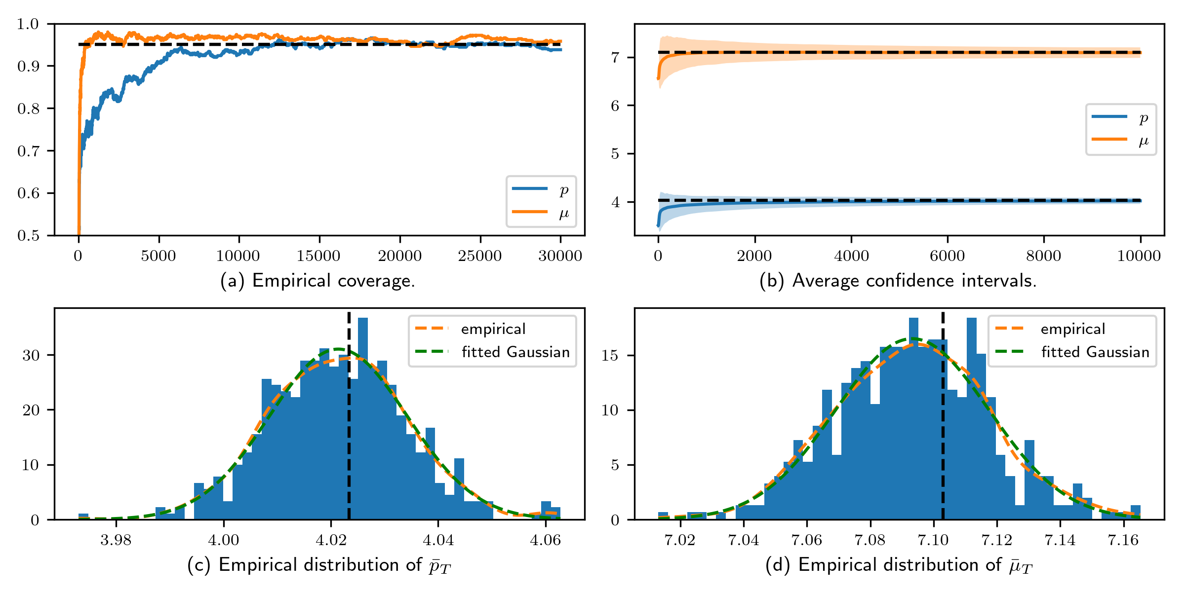
Figure 12: Online inference for M/M/1 queues over 500 repetitions with $\alpha=1$.

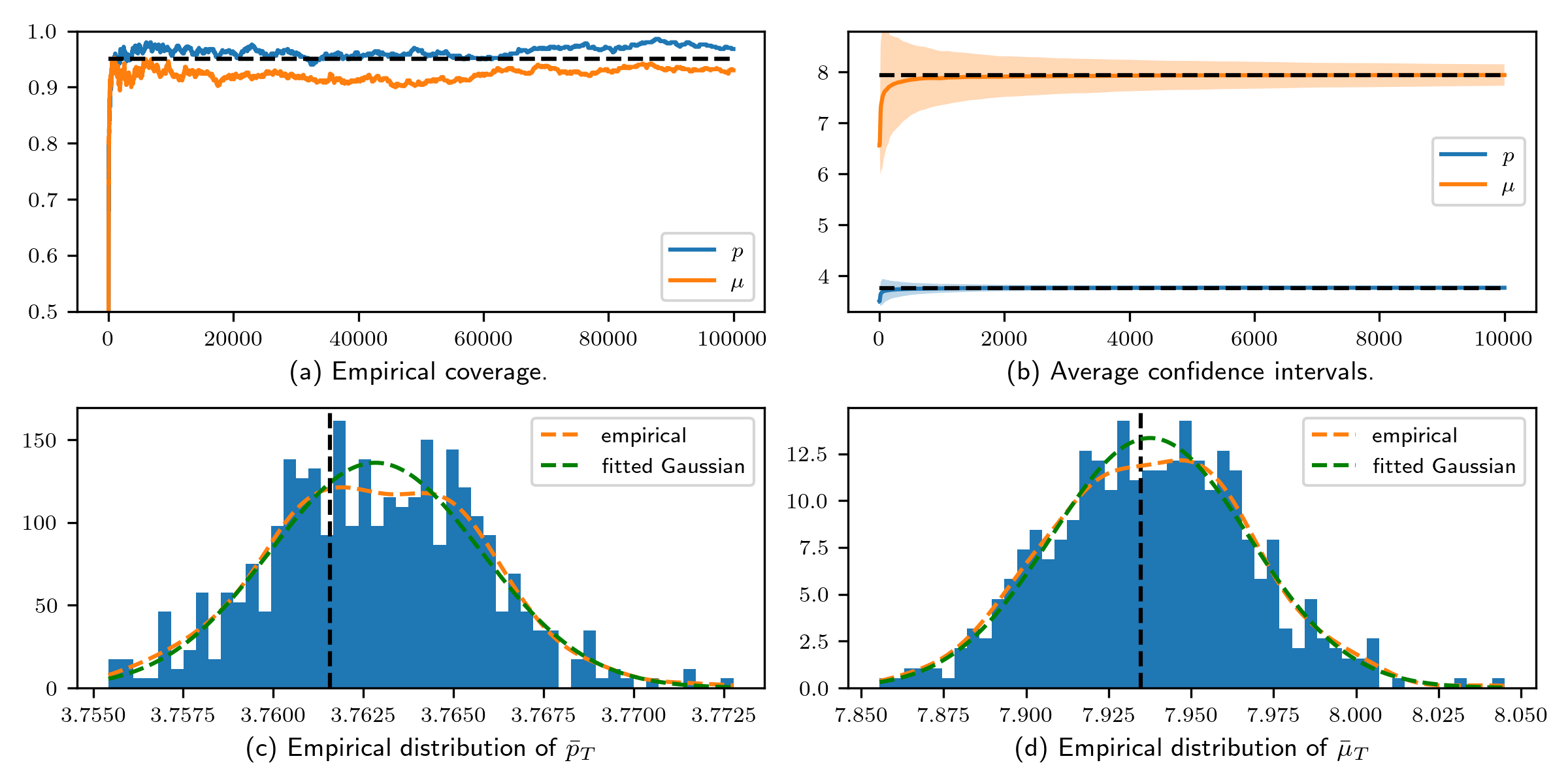
Figure 13: Online inference for GI/M/1 queues over 500 repetitions with $\alpha=1$.

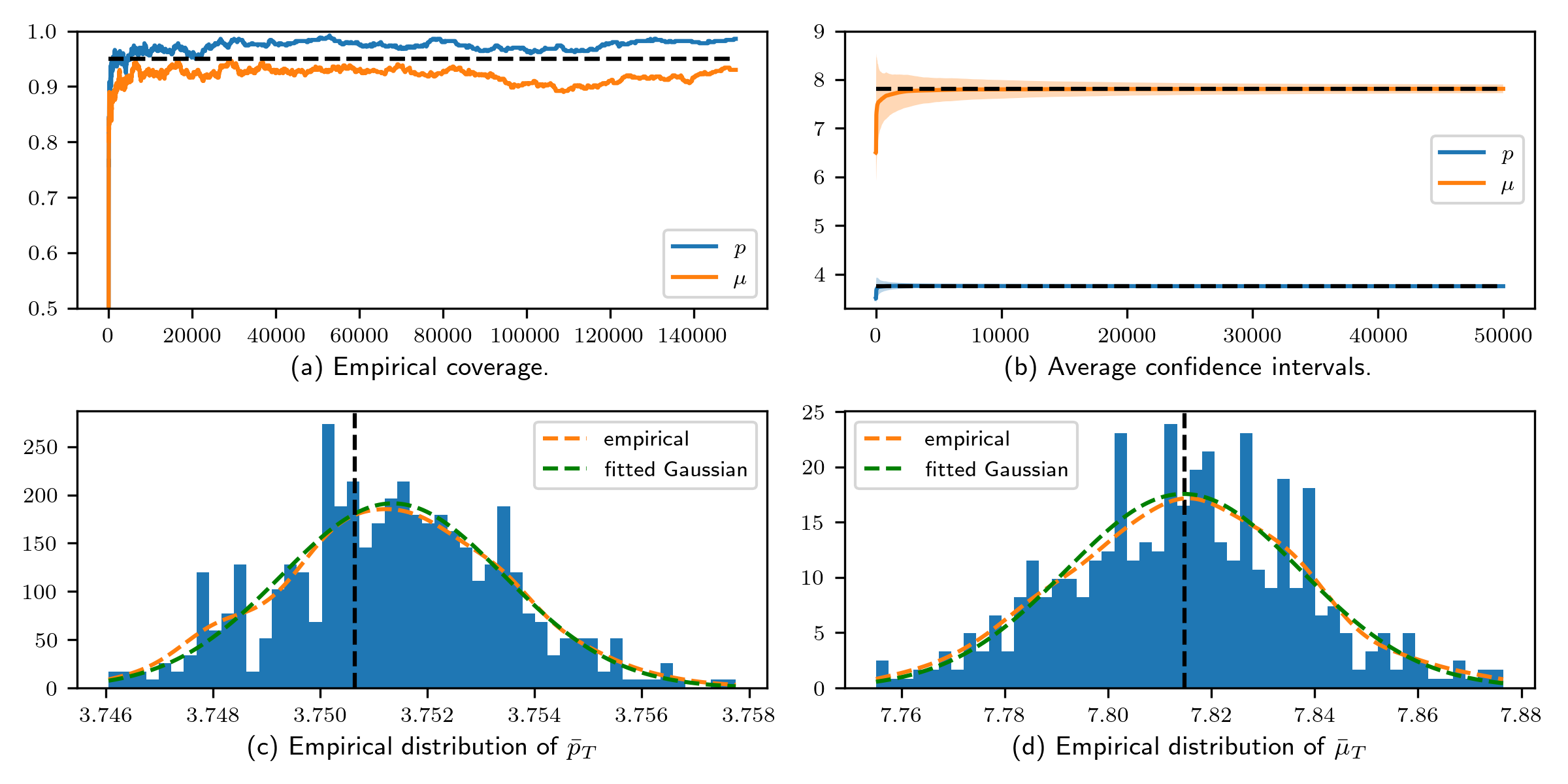
Figure 14: Online inference for M/GI/1 queues with $c_{s}=0.5$ over 500 repetitions with $\alpha=1$.

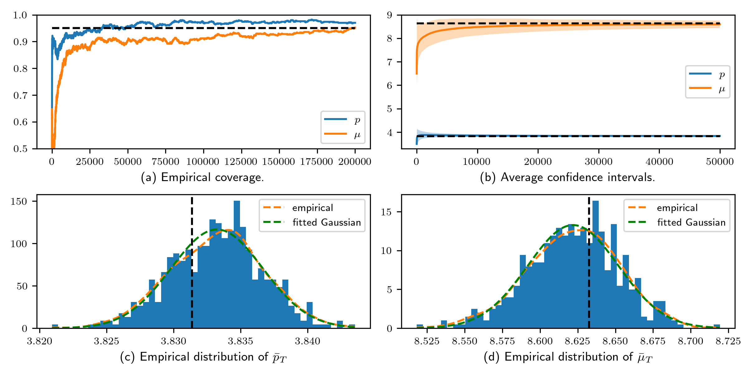
Figure 15: Online inference for M/GI/1 queues with $c_{s}=1.5$ over 500 repetitions with $\alpha=1$.

Appendix F Proof Sketch of Theorem 1

A major advancement of our work compared to GOLiQ is the improvement of efficiency on searching optimizer ${\vartheta^{\star}}$. This is primarily attributed to the convergence analysis framework we are about to introduce for SAMCMC. Our analysis on $\Delta_{t}$ starts with the recursion:

$${\mathbb{E}}\left\|\vartheta_{t+1}-{\vartheta^{\star}}\right\|^{2} ={\mathbb{E}}\left\|\Pi\left(\vartheta_{t}-\eta_{t}H(\vartheta_{t},x_{t})\right)-{\vartheta^{\star}}\right\|^{2}$$

$$\leq{\mathbb{E}}\left\|\vartheta_{t}-{\vartheta^{\star}}-\eta_{t}H(\vartheta_{t},x_{t})\right\|^{2}$$

$$={\mathbb{E}}\left\|\vartheta_{t}-{\vartheta^{\star}}\right\|^{2}-\,2\eta_{t}{\mathbb{E}}\langle\vartheta_{t}-{\vartheta^{\star}},H(\vartheta_{t},x_{t})\rangle+\eta_{t}^{2}{\mathbb{E}}\left\|H(\vartheta_{t},x_{t})\right\|^{2}$$

$$\leq\left(1-2\eta_{t}K_{0}\right){\mathbb{E}}\left\|\vartheta_{t}-{\vartheta^{\star}}\right\|^{2}+K\eta_{t}^{2}-2\eta_{t}{\mathbb{E}}\left\langle\vartheta_{t}-{\vartheta^{\star}},H(\vartheta_{t},x_{t})-g(\vartheta_{t})\right\rangle.$$

To simplify the notation, we define $G_{m:n}=\prod_{t=m}^{n}(1-2\eta_{t}K_{0})$, for $n>m\geq 1$, and $G_{m:n}=1$ if $n\leq m$. Then, we have

$$\Delta_{t+1} \textstyle\leq G_{1:t}\Delta_{1}+K\sum_{s=1}^{t}G_{s+1:t}\eta_{s}^{2}+2\sum_{s=1}^{t}G_{s+1:t}\eta_{s}{\mathbb{E}}\left\langle{\vartheta^{\star}}-\vartheta_{s},H(\vartheta_{s},x_{s})-g(\vartheta_{s})\right\rangle.$$ (60)

Our ultimate goal is to show that $\Delta_{t+1}=O(\eta_{t})$. It is then sufficient to show that each of the three terms on the right hand side of Equation 60 are of order $O(\eta_{t})$. The first term $G_{1:t}\Delta_{1}$ denotes the optimization error arising from the initialization. Under Condition $(b)$ of Assumption 4, it can be verified that $\eta_{t}\geq t^{-1}/(2K_{0})$. This leads to the inequality

$$G_{1:t}=\prod_{\tau=1}^{t}(1-2\eta_{t}K_{0})\leq\exp\left\{2K_{0}\sum_{\tau=1}^{t}\eta_{t}\right\}\leq\exp\left\{\sum_{\tau=1}^{t}t^{-1}\right\}=O(t^{-1})=O(\eta_{t}),$$

which effectively renders the optimization error manageable and controllable. The second term $K\sum_{s=1}^{t}G_{s+1:t}\eta_{s}^{2}$ accounts the variance in the random estimators $H(\vartheta_{s},x_{s+1})$ for $g(\vartheta_{s})$. Given Assumption 4, the following lemma shows that $K\sum_{s=1}^{t}G_{s+1:t}\eta_{s}^{2}=O(\eta_{t})$.

Lemma 20.

Let $a>0$ and $\{\eta_{t}\}_{t\geq 1}$ be a non-increasing sequence such that $\eta_{1}<2/a$. If $\eta_{t-1}/\eta_{t}\leq 1+(a/2)\eta_{t}$ for any $k\geq 1$, then for any $t\geq 2$,

$$\sum_{s=1}^{t}\eta_{s}^{2}\prod_{\tau=s+1}^{t}\left(1-\eta_{\tau}a\right)\leq\frac{2}{a}\eta_{t}.$$

The proof of Lemma 20 is similar to the analysis in (Polyak and Juditsky, 1992; Moulines and Bach, 2011; Chen et al., 2020; Li et al., 2023a). Actually, the first two terms also appear in finite-step analysis for standard SA algorithm with unbiased estimators for $g(\vartheta)$.
Therefore, the most challenging step in our convergence analysis lies in the cross term

$$\sum_{s=1}^{t}G_{s+1:t}\eta_{s}{\mathbb{E}}\left\langle{\vartheta^{\star}}-\vartheta_{s},H(\vartheta_{s},x_{s})-g(\vartheta_{s})\right\rangle,$$

which is unique to SAMCMC. To bound the cross terms, we make use of the Poisson equation to decompose the gradient error $H(\vartheta_{s},x_{s})-g(\vartheta_{s})$ into martingale and finite difference terms. Our analysis approach is inspired by Benveniste et al. (2012) and has recently been used by Atchadé et al. (2017); Karimi et al. (2019); Li and Wai (2022) for the finite-time convergence analysis of different algorithms. Under the ergodicity conditions in Assumption LABEL:assmpt:_uniform_ergodicity, it is known that there exists a unique bivariate function $U(\vartheta,x)$ for $\vartheta\in\Theta$ and $x\in\mathcal{X}$ solving the Poisson equation

$$H(\vartheta,x)-g(\vartheta)=U(\vartheta,x)-P_{\vartheta}U(\vartheta,x),$$

where $P_{\vartheta}U(\vartheta,x)\equiv\int_{\mathcal{X}}U(\vartheta,x^{\prime})P_{\vartheta}(x,dx^{\prime})$. Our first observation is that $U(\vartheta,x)$ is continuous in $\vartheta$ under the technical assumptions we imposed on $\{P_{\vartheta}:\vartheta\in\Theta\}$.

Proposition 5 (Continuity of $U(\vartheta,x)$).

For any $x\in\mathcal{X}$ and $\vartheta,\vartheta^{\prime}\in\Theta$, we have that

$$\|P_{\vartheta}U(\vartheta,x)-P_{\vartheta^{\prime}}U(\vartheta^{\prime},x)\|\leq L_{U}(x)\cdot\|\vartheta-\vartheta^{\prime}\|.$$

Moreover the function $L_{U}(x)$ satisfies

$$\mathbb{E}[L^{2}_{U}(x_{t})]\leq C_{U},$$

for some universal constant $C_{U}>0$. Explain the distribution of $x_{t}$ here.

In addition, we have the following uniform bound on the expectation of $P_{\vartheta_{t}}U(\vartheta_{t},x_{t})$:

Lemma 21 (Uniform Bound on $P_{\vartheta_{t}}U(\vartheta_{t},x_{t})$).

Under Assumptions LABEL:assmpt:_uniform_ergodicity and LABEL:assmpt:_uniform_bound, then for any adaptive sequence $\{\vartheta_{t}\}$,

$$\mathbb{E}[(P_{\vartheta_{t}}U(\vartheta_{t},x_{t}))^{{\color[rgb]{1,0,0}2}}]\leq K,$$

where $K>0$ is a universal constant.

For each $1\leq s\leq t$, given the solution $U(\vartheta_{s},x_{s})$, we can decompose

$$H(\vartheta_{s},x_{s})-g(\vartheta_{s})$$

$$=~{} \left[U(\vartheta_{s},x_{s})-P_{\vartheta_{s}}U(\vartheta_{s},x_{s-1})\right]+\left[P_{\vartheta_{s}}U(\vartheta_{s},x_{s-1})-P_{\vartheta_{s}}U(\vartheta_{s},x_{s})\right],$$

where $U(\vartheta_{s},x_{s})-P_{\vartheta_{s}}U(\vartheta_{s},x_{s-1})$ is a martingale difference and cancels out by taking expectation. Consequently, we can simplify the cross-term to the ‘pure’ residual term as

$$\sum_{s=1}^{t}G_{s+1:t}\eta_{s}\mathbb{E}\left[\langle\vartheta-\vartheta_{s},H(\vartheta_{s},x_{s})-g(\vartheta_{s})\rangle\right]$$

$$=\sum_{s=1}^{t}G_{s+1:t}\eta_{s}\mathbb{E}\left[\langle{\vartheta^{\star}}-\vartheta_{s},P_{\vartheta_{s}}U(\vartheta_{s},x_{s-1})-P_{\vartheta_{s}}U(\vartheta_{s},x_{s})\rangle\right].$$

To bound the ‘pure’ residual term, we shall utilize Proposition 5 and break it down into four terms $\{A_{i}\}_{i\in[4]}$ as follows

$$\sum_{s=1}^{t}G_{s+1:t}\eta_{s}{\mathbb{E}}\left\langle{\vartheta^{\star}}-\vartheta_{s},P_{\vartheta_{s}}U(\vartheta_{s},x_{s-1})-P_{\vartheta_{s}}U(\vartheta_{s},x_{s})\right\rangle]=A_{1}+A_{2}+A_{3}+A_{4},$$

where

$$A_{1}:=-\sum_{s={\color[rgb]{1,0,0}2}}^{t}\eta_{s}G_{s+1:t}{\mathbb{E}}\left\langle\vartheta_{s}-{\vartheta^{\star}},P_{\vartheta_{s}}U(\vartheta_{s},x_{s-1})-P_{\vartheta_{s-1}}U(\vartheta_{s-1},x_{s-1})\right\rangle$$

$$A_{2}:=-\sum_{s=2}^{t}\eta_{s}G_{s+1:t}{\mathbb{E}}\left\langle\vartheta_{s}-\vartheta_{s-1},P_{\vartheta_{s-1}}U(\vartheta_{s-1},x_{s-1})\right\rangle$$

$$A_{3}:=-\sum_{s=2}^{t}(\eta_{s}G_{s+1:t}-\eta_{s-1}G_{s:t}){\mathbb{E}}\left\langle\vartheta_{s-1}-{\vartheta^{\star}},P_{\vartheta_{s-1}}U(\vartheta_{s-1},x_{s-1})\right\rangle$$

$$A_{4}:=-\eta_{1}G_{2:t}{\mathbb{E}}\left\langle\vartheta_{1}-{\vartheta^{\star}},P_{\vartheta_{1}}U(\vartheta_{1},x_{0})\right\rangle+\eta_{t}{\mathbb{E}}\left\langle\vartheta_{t}-{\vartheta^{\star}},P_{\vartheta_{t}}U(\vartheta_{t},x_{t})\right\rangle.$$

We explain our main idea of treatment on $A_{1}$ to $A_{4}$:

• $A_{1}$: Based on Proposition 5 and the fact that $|\eta_{s}-\eta_{s-1}|=O(\eta_{s})$, we can conclude that $A_{1}$ has the same order as $\sum_{s=1}^{t}G_{s+1:t}\eta_{s}^{2}$ and thus should of order $O(\eta_{t})$ following Lemma 20.

• $A_{2}$: The difference $\vartheta_{s}-\vartheta_{s-1}$ introduces an extra $\eta_{s}$ term inside the summation. Given Lemma 21, the rest of analysis is similar to the treatment of $A_{1}$.

• $A_{3}$: Following Assumption 4, we obtain $|\eta_{s}G_{s+1:t}-\eta_{s-1}G_{s:t}|=???$ and therefore $???$.

• $A_{4}$: It follows immediately from the result that $G_{2:t}=O(\eta_{t})$.

Thus we can conclude that the ‘pure’ residual term is also of order $O(\eta_{t})$, which closes the proof of Theorem 1.

References

- Abadir and Paruolo [1997] Karim M Abadir and Paolo Paruolo. Two mixed normal densities from cointegration analysis. Econometrica: Journal of the Econometric Society, pages 671–680, 1997.
- Andrieu and Moulines [2006] C. Andrieu and É. Moulines. On the ergodicity property of some adaptive MCMC algorithms. The annals of Applied Probability, 16:1462–1505, 2006.
- Atchadé and Liu [2010] Yves F Atchadé and Jun S Liu. The Wang-Landau algorithm in general state spaces: Applications and convergence analysis. Statistica Sinica, pages 209–233, 2010.
- Atchadé et al. [2017] Yves F Atchadé, Gersende Fort, and Eric Moulines. On perturbed proximal gradient algorithms. The Journal of Machine Learning Research, 18(1):310–342, 2017.
- Benveniste et al. [2012] Albert Benveniste, Michel Métivier, and Pierre Priouret. Adaptive algorithms and stochastic approximations, volume 22. Springer Science & Business Media, 2012.
- Borkar [2009] Vivek S Borkar. Stochastic approximation: A dynamical systems viewpoint, volume 48. Springer, 2009.
- Chen et al. [2020] Xi Chen, Jason D Lee, Xin T Tong, and Yichen Zhang. Statistical inference for model parameters in stochastic gradient descent. The Annals of Statistics, 48(1):251–273, 2020.
- Chen et al. [2021] Xi Chen, Zehua Lai, He Li, and Yichen Zhang. Online statistical inference for stochastic optimization via Kiefer-Wolfowitz methods. arXiv e-prints, pages arXiv–2102, 2021.
- Chen et al. [2023] Xinyun Chen, Yunan Liu, and Guiyu Hong. An online learning approach to dynamic pricing and capacity sizing in service systems. Operations Research, 2023.
- Chong and Ramadge [1994] E. K. P. Chong and P. J. Ramadge. Stochastic optimization of regenerative systems using infinitesimal perturbation analysis. IEEE Transactions on Automatic Control, 39:1400–1410, 1994.
- Durrett [2013] Rick Durrett. Probability: Theory and Examples (Edition 4.1). Cambridge University Press, 2013.
- Fang et al. [2018] Yixin Fang, Jinfeng Xu, and Lei Yang. Online bootstrap confidence intervals for the stochastic gradient descent estimator. The Journal of Machine Learning Research, 19(1):3053–3073, 2018.
- Fu [1990] M. C. Fu. Convergence of a stochastic approximation algorithm for the GI/G/1 queue using infinitesimal perturbation analysis. Journal of Optimization Theory and Applications, 65:149–160, 1990.
- Glynn and Meyn [1996] Peter W Glynn and Sean P Meyn. A liapounov bound for solutions of the poisson equation. The Annals of Probability, pages 916–931, 1996.
- Gu and Kong [1998] Ming Gao Gu and Fan Hui Kong. A stochastic approximation algorithm with Markov chain Monte-Carlo method for incomplete data estimation problems. Proceedings of the National Academy of Sciences, 95(13):7270–7274, 1998.
- Gu and Zhu [2001] Ming Gao Gu and Hong-Tu Zhu. Maximum likelihood estimation for spatial models by Markov chain Monte Carlo stochastic approximation. Journal of the Royal Statistical Society Series B: Statistical Methodology, 63(2):339–355, 2001.
- Hall and Heyde [2014] Peter Hall and Christopher C Heyde. Martingale limit theory and its application. Academic press, 2014.
- Huh et al. [2009] W. T. Huh, G. Janakiraman, J. A. Muckstadt, and P. Rusmevichientong. An adaptive algorithm for finding the optimal base-stock policy in lost sales inventory system with censored demand. Mathematics of Operations Research, 34(2):397–416, 2009.
- Jia et al. [2022] Huiwen Jia, Cong Shi, and Siqian Shen. Online learning and pricing for service systems with reusable resources. Operations Research, 0(0):null, 2022.
- Karimi et al. [2019] Belhal Karimi, Blazej Miasojedow, Eric Moulines, and Hoi-To Wai. Non-asymptotic analysis of biased stochastic approximation scheme. In Conference on Learning Theory, pages 1944–1974. PMLR, 2019.
- Kiefer et al. [2000] Nicholas M Kiefer, Timothy J Vogelsang, and Helle Bunzel. Simple robust testing of regression hypotheses. Econometrica, 68(3):695–714, 2000.
- Kurtz [2005] Thomas G Kurtz. Averaging for martingale problems and stochastic approximation. In Applied Stochastic Analysis: Proceedings of a US-French Workshop, Rutgers University, New Brunswick, NJ, April 29–May 2, 1991, pages 186–209. Springer, 2005.
- Kushner and Yin [2003] Harold Kushner and G George Yin. Stochastic approximation and recursive algorithms and applications, volume 35. Springer Science & Business Media, 2003.
- L’Ecuyer and Glynn [1994] P. L’Ecuyer and P. W. Glynn. Stochastic optimization by simulation: Convergence proofs for the GI/GI/1 queue in steady state. Management Science, 40(11):1562–1578, 1994.
- L’Ecuyer et al. [1994] P. L’Ecuyer, N. Giroux, and P. W. Glynn. Stochastic optimization by simulation: Numerical experiments with the M/M/1 queue in steady-state. Management Science, 40(10):1245–1261, 1994.
- Lee et al. [2022a] Sokbae Lee, Yuan Liao, Myung Hwan Seo, and Youngki Shin. Fast and robust online inference with stochastic gradient descent via random scaling. In the AAAI Conference on Artificial Intelligence, volume 36, pages 7381–7389, 2022a.
- Lee et al. [2022b] Sokbae Lee, Yuan Liao, Myung Hwan Seo, and Youngki Shin. Fast inference for quantile regression with tens of millions of observations. Available at SSRN 4263158, 2022b.
- Li and Wai [2022] Qiang Li and Hoi-To Wai. State dependent performative prediction with stochastic approximation. In International Conference on Artificial Intelligence and Statistics, pages 3164–3186. PMLR, 2022.
- Li et al. [2018] Tianyang Li, Liu Liu, Anastasios Kyrillidis, and Constantine Caramanis. Statistical inference using SGD. In the AAAI Conference on Artificial Intelligence, volume 32, 2018.
- Li et al. [2022] Xiang Li, Jiadong Liang, Xiangyu Chang, and Zhihua Zhang. Statistical estimation and online inference via Local SGD. In Po-Ling Loh and Maxim Raginsky, editors, Conference on Learning Theory, volume 178, pages 1613–1661. PMLR, 2022.
- Li et al. [2023a] Xiang Li, Jiadong Liang, and Zhihua Zhang. Online statistical inference for nonlinear stochastic approximation with markovian data. arXiv preprint arXiv:2302.07690, 2023a.
- Li et al. [2023b] Xiang Li, Wenhao Yang, Zhihua Zhang, and Michael I Jordan. A statistical analysis of Polyak-Ruppert averaged Q-Learning. In International Conference on Artificial Intelligence and Statistics, volume 206, 2023b.
- Liang [2010] Faming Liang. Trajectory averaging for stochastic approximation MCMC algorithms. The Annals of Statistics, 38(5):2823–2856, 2010.
- Liang et al. [2007] Faming Liang, Chuanhai Liu, and Raymond J Carroll. Stochastic approximation in Monte Carlo computation. Journal of the American Statistical Association, 102(477):305–320, 2007.
- Liang and Su [2019] Tengyuan Liang and Weijie J Su. Statistical inference for the population landscape via moment-adjusted stochastic gradients. Journal of the Royal Statistical Society, 2019.
- Liu et al. [2022] Yi Liu, Ke Sun, Bei Jiang, and Linglong Kong. Identification, amplification and measurement: A bridge to gaussian differential privacy. In Advances in Neural Information Processing Systems, volume 35, pages 11410–11422, 2022.
- Ma et al. [2015] Yi-An Ma, Tianqi Chen, and Emily Fox. A complete recipe for stochastic gradient MCMC. Advances in neural information processing systems, 28, 2015.
- Moulines and Bach [2011] Eric Moulines and Francis Bach. Non-asymptotic analysis of stochastic approximation algorithms for machine learning. Advances in neural information processing systems, 24, 2011.
- Moyeed and Baddeley [1991] RA Moyeed and Adrian J Baddeley. Stochastic approximation of the MLE for a spatial point pattern. Scandinavian Journal of Statistics, pages 39–50, 1991.
- Nemeth and Fearnhead [2021] Christopher Nemeth and Paul Fearnhead. Stochastic gradient Markov chain Monte Carlo. Journal of the American Statistical Association, 116(533):433–450, 2021.
- Polyak and Juditsky [1992] Boris T Polyak and Anatoli B Juditsky. Acceleration of stochastic approximation by averaging. SIAM journal on control and optimization, 30(4):838–855, 1992.
- Ramprasad et al. [2021] Pratik Ramprasad, Yuantong Li, Zhuoran Yang, Zhaoran Wang, Will Wei Sun, and Guang Cheng. Online bootstrap inference for policy evaluation in reinforcement learning. Journal of the American Statistical Association, 2021.
- Ravner and Snitkovsky [2023] Liron Ravner and Ran I. Snitkovsky. Stochastic approximation of symmetric Nash equilibria in queueing games. Operations Research, 0(0):null, 2023.
- Robbins and Siegmund [1971] Herbert Robbins and David Siegmund. A convergence theorem for non-negative almost supermartingales and some applications. In Optimizing methods in statistics, pages 233–257. Elsevier, 1971.
- Su and Zhu [2023] Weijie J Su and Yuancheng Zhu. Higrad: Uncertainty quantification for online learning and stochastic approximation. Journal of Machine Learning Research, 24(124):1–53, 2023.
- Suri and Zazanis [1988] Rajan Suri and Michael A Zazanis. Perturbation analysis gives strongly consistent sensitivity estimates for the M/G/1 queue. Management Science, 34(1):39–64, 1988.
- Toulis and Airoldi [2017] Panos Toulis and Edoardo M Airoldi. Asymptotic and finite-sample properties of estimators based on stochastic gradients. The Annals of Statistics, 45(4):1694–1727, 2017.
- Whitt [2007] Ward Whitt. Proofs of the martingale FCLT. Probability Surveys, 4:268–302, 2007.
- Yuan et al. [2021] Hao Yuan, Qi Luo, and Cong Shi. Marrying stochastic gradient descent with bandits: Learning algorithms for inventory systems with fixed costs. Management Science, 67(10):6089–6115, 2021.
- Zhang et al. [2020] Huanan Zhang, Xiuli Chao, and Cong Shi. Closing the gap: A learning algorithm for lost-sales inventory systems with lead times. Management Science, 66(5):1962–1980, 2020.
- Zhu et al. [2021] Wanrong Zhu, Xi Chen, and Wei Biao Wu. Online covariance matrix estimation in stochastic gradient descent. Journal of the American Statistical Association, pages 1–12, 2021.