Opacities of Dense Gas Tracers In Galactic Massive Star Forming Regions

Shu Liu,¹ Junzhi Wang,² Fei Li,^3,4 Jingwen Wu,^5,1 Zhi-Yu Zhang,^3,4 Di Li,^1,6,7 Ningyu Tang,⁸ and Pei Zuo^1,9
¹National Astronomical Observatories, Chinese Academy of Sciences, Beijing 100101, People’s Republic of China
²Guangxi Key Laboratory for Relativistic Astrophysics, Department of Physics, Guangxi University, Nanning 530004, People’s Republic of China
³School of Astronomy and Space Science, Nanjing University, Nanjing 210023, People’s Republic of China
⁴Key Laboratory of Modern Astronomy and Astrophysics (Nanjing University), Ministry of Education, Nanjing 210023, People’s Republic of China
⁵University of Chinese Academy of Sciences, Beijing 100049, People’s Republic of China
⁶Key Laboratory of Radio Astronomy and Technology, Chinese Academy of Sciences, Beijing 100101, People’s Republic of China
⁷Research Center for Intelligent Computing Platforms, Zhejiang Laboratory, Hangzhou 311100, People’s Republic of China
⁸Department of Physics, Anhui Normal University, Wuhu, Anhui 241002, People’s Republic of China
⁹Kavli Institute for Astronomy and Astrophysics, Peking University, Beijing 100871, People’s Republic of China
E-mail: liushu@nao.cas.cnE-mail: junzhiwang@gxu.edu.cn

(Accepted 2023 August 08. Received 2023 July 13; in original form 2022 June 09)

Abstract

Optical depths of dense molecular gas are commonly used in Galactic and extragalactic studies to constrain the dense gas mass of the clouds or galaxies. The optical depths are often obtained based on spatially unresolved data, especially in galaxies, which may affect the reliability of such measurements. We examine such effects in spatially resolved Galactic massive star forming regions. Using the 10-m SMT telescope, we mapped HCN and H¹³CN 3-2, HCO⁺ and H¹³CO⁺ 3-2 toward 51 Galactic massive star forming regions, 30 of which resulted in robust determination of spatially-resolved optical depths. Conspicuous spatial variations of optical depths have been detected within each source. We first obtained opacities for each position and calculated an optical-thick line intensity-weighted average, then averaged all the spectra and derived a single opacity for each region. The two were found to agree extremely well, with a linear least square correlation coefficient of 0.997 for the whole sample.

keywords:

galaxies: ISM – ISM: clouds – ISM: molecules – opacity

^†^†pubyear: 2023^†^†pagerange: Opacities of Dense Gas Tracers In Galactic Massive Star Forming Regions–A

1 Introduction

Dense molecular gas is a key to understand star formation in galaxies. Observations have demonstrated that stars, especially massive stars, are essentially and exclusively formed in the dense cores of giant molecular cores (GMCs, Evans, 2008). Low- $J$ CO lines trace the total amount of molecular gas content, not sensitive to the dense cores with volume densities higher than 10⁴ cm^-3 . The transitions of molecules with large dipole moment, such as HCN, HCO⁺, HNC, and CS, which have high critical density $n_{\rm crit}>10^{4}$ cm^-3 , are tracers of dense gas. With observations of HCN 1-0 toward 65 galaxies, Gao & Solomon (2004) found a strong linear correlation between the luminosities of HCN 1-0 and Infrared emission. This correlation was found to extend to Galactic dense cores (e.g. Wu, et al., 2005), and possibly to high- $z$ galaxies and QSOs as well (e.g. Gao, et al., 2007). Further observations of CS $J$ =5-4 in 24 IR-bright galaxies show such linear correlation still valid for the gas as dense as $n_{\rm H_{2}}\sim 10^{6}$ cm^-3 (Wang, Zhang & Shi, 2011), which was supported by HCN 4-3 and CS 7-6 survey toward 20 nearby star-forming galaxies (Zhang, et al., 2014). Multiple line single pointing observations of HCN 1-0, HCO⁺ 1-0, HNC 1-0, and CS 3-2 toward a sample of 70 galaxies also showed similar linear relationships (Li et al., 2021). Spatially resolved observations for local galaxies were also performed to study dense gas fraction and related star formation, such as, HCN 1-0, HCO⁺ 1-0, CS 2-1, ¹³CO 1-0, and C¹⁸O toward inner region of four local galaxies with ALMA and IRAM 30 m (Gallagher et al., 2018), HCN 1-0, HCO⁺ 1-0, HNC 1-0, and CO isotopologues toward a number of nearby galaxies in the IRAM large program EMPIRE (Cormier et al., 2018; Jiménez-Donaire et al., 2017b, 2019), HCN 1-0 and CO 1-0 toward M51 with the 50 meter Large millimeter telescope (LMT) (Heyer et al., 2022), and CO isotopologues investigation within the CLAWS programme (den Brok et al., 2022).

However, because of the large dipole moments and high column density, such dense gas tracers are normally optically thick both in Galactic GMC cores and in galaxies. It is of any case hard to convert from luminosity of these tracers to dense gas mass, which is similar to the issue of the standard conversion factor of CO with several times or even more than 10 times uncertainty in different galaxies (e.g., Narayanan, et al., 2012; Papadopoulos, et al., 2012). Multiple transitions of molecular lines are powerful to derive the physical properties (volume density, temperature, etc.) of dense gas in galaxies, which had been made for nearby starbursts and ULIRGs (e.g., M 82, NGC 253 in Nguyen, et al. 1992, ARP 220, NGC 6240 in Greve, et al. 2009), with large uncertainties.

Optically thin dense gas tracers, such as isotopic lines, are necessary for better understanding dense gas properties and chemical evolution in the Galaxy (Langer & Penzias, 1990; Wilson & Matteucci, 1992; Wilson & Rood, 1994; Henkel et al., 1994; Milam et al., 2005). In recent years, increasing studies of CO isotopologues have been carried out in other galaxies (Martín et al., 2010; Henkel et al., 2014; Meier et al., 2015; Jiménez-Donaire et al., 2017a, b, 2019; Cormier et al., 2018; den Brok et al., 2021). Assuming a reasonable isotopic abundance ratio, one can determine the optical depths of dense gas tracers, such as HCN and CS lines, with the intensity ratio of dense gas tracers and their isotopic lines (Wang et al., 2014, 2016; Li, et al., 2020). However, despite the uncertainty of isotopic abundance in different galaxies, there are still other problems for determining the optical depths of dense gas tracers. One important effect is that we can only assume one value of optical depth in one galaxy if we do not have spatial resolution, while optical depths should vary at different regions, which had been seen in M 82 along major axis (Li et al., 2022).

Thus, the derived optical depth of one dense gas tracer in each galaxy with one pair of dense gas tracer and its isotopic line, is only an averaged value within the observed region. Since it is a non-linear relation between optical depth and line ratio, the typical optical depth in one region with internal spatial distribution of different optical depth, may not be well constrained by line ratio of spatially integrated fluxes for both dense gas tracer and its isotopic line. The best way to study this effect is mapping a sample of massive star forming regions in the Milky Way with both dense gas tracers and their isotopic lines. The detailed description for deriving optical depths with two ways will be presented in Section 3.

In this paper, the observations and data reduction are described in Section 2, while the methods of calculating optical depths in each sources are presented in Section 3. Then, the main results and discussions are given in Section4 and Section 5, and a brief summary is presented in Section 6.

2 Observations and data reduction

The sample presented in this study is a subset of massive star forming regions with parallax distances from Reid, et al. (2014) with strong ( $>$ 0.5 K) H¹³CN 2-1 emissions, which was detected by the Institut de Radioastronomie Millimétrique (IRAM) 30-m telescope in June and October 2016 (Wang et al., in preparation), for the guarantee of strong H¹³CN 3-2 emission.

The observations were carried out using the Arizona Radio Observatory (ARO) 10-m Submillimeter Telescope (SMT) on Mt. Graham, Arizona, during several observing runs in 2017 March to May, 2017 December, 2018 January, 2018 March, 2018 May and 2018 October to November. Four molecular lines were observed with 1.3 mm ALMA band 6 receiver. HCN 3-2 with rest frequency of 265.886431 GHz and HCO⁺ 3-2 with rest frequency of 267.557633 GHz were tuned in the upper sideband (USB) simultaneously. The isotopologues, H¹³CN 3-2 with rest frequency of 259.011787 GHz and H¹³CO⁺ 3-2 with rest frequency of 260.255342 GHz were observed simultaneously also in the upper sideband (USB). The Forbes Filter Banks (FFB) backend was setup with 512 -MHz bandwidth for each line and 1 MHz channel spacing, which corresponds to $\sim$ 1.15 km s^-1 at 260 GHz, with the spatial resolution of $\sim$ 27.8^′′.

For each source, the on-the-fly (OTF) mode was used to cover 2 ${}^{\prime}\times 2^{\prime}$ regions for HCN and HCO⁺ 3-2, and 1.5 ${}^{\prime}\times 1.5^{\prime}$ for H¹³CN and H¹³CO⁺ 3-2, respectively (Table 1). The telescope time on each source for the tuning of HCN and HCO⁺ 3-2 is around 40 minutes for most of the samples except for 9 sources as 80 minutes. For the isotopologues, the time on the strong ones are about 1.5 hours or 3 hours while on the other moderately weak cores are about 4.5 hours, even up to 6 hours for two cores due to the weather conditions. The off points were chosen as azimuth off 30^′ away from the mapping centers. The observation information as on-source time, system temperatures ( $T_{\rm sys}$ ) and rms of HCN and H¹³CN 3-2 for each source are shown in Table 2. The information of HCO⁺ 3-2 and H¹³CO⁺ 3-2 are not exhibited, since what are comparable to those of HCN and H¹³CN 3-2, respectively.

The OTF data of HCN and HCO⁺ 3-2 for each source were re-gridded to the final maps with the step of 15^′′. The map of H¹³CN and H¹³CO⁺ 3-2 are gridded to match the center and each position of the spatially resolved HCN and HCO⁺ 3-2 data, respectively. The antenna temperature $T_{A}^{*}$ was converted to main beam brightness temperature $T_{mb}$ using $T_{mb}=T_{A}^{*}/{\eta}_{b}$ . The main beam efficiency ${\eta}_{b}$ is 0.77. Typical noise levels were 0.09 K for HCN and HCO⁺ 3-2, as well as 0.03 K for H¹³CO⁺ 3-2 at the frequency spacing of 1 MHz in the unit of $T_{A}^{*}$ , respectively.

A total of 51 sources were mapped. However, only sources with enough spatially resolved data points to obtained reliable H¹³CN and H¹³CO⁺ 3-2 signals, are selected for final analysis. The selected 30 sources with basic parameters are listed in Table 1. All of the data were reduced with the CLASS software package in GILDAS¹¹1http://www.iram.fr/IRAMFR/GILDAS. For each line of each source, we first took a quick look at main regions with emission and obtained an averaged spectrum within this region to determine the line velocity range. Such velocity ranges were used as “mask” with “set window” in CLASS when baseline subtractions were done with first order polynomial. Then we used “print area” in CLASS to obtain the velocity integrated fluxes for each pixel, with the same value used for baseline subtraction, which was fixed the spectra within the map for each line of each source.

Table 1: Sample of high mass star forming regions.

source name	Alias	RA(J2000)	DEC(J2000)	D	D_GC	$v_{\rm LSR}$
				kpc	kpc	km s^-1
G005.88-00.39		18:00:30.31	-24:04:04.50	3.0	5.3	9.3
G009.62+00.19		18:06:14.66	-20:31:31.70	5.2	3.3	4.8
G010.47+00.02		18:08:38.23	-19:51:50.30	8.5	1.6	65.7
G010.62-00.38	W 31	18:10:28.55	-19:55:48.60	5.0	3.6	4.3
G011.49-01.48		18:16:22.13	-19:41:27.20	1.2	7.1	10.5
G011.91-00.61		18:13:58.12	-18:54:20.30	3.4	5.1	36.1
G012.80-00.20		18:14:14.23	-17:55:40.50	2.9	5.5	36.3
G014.33-00.64		18:18:54.67	-16:47:50.30	1.1	7.2	22.6
G015.03-00.67	M 17	18:20:24.81	-16:11:35.30	2.0	6.4	19.7
G016.58-00.05		18:21:09.08	-14:31:48.80	3.6	5.0	60.0
G023.00-00.41		18:34:40.20	-09:00:37.00	4.6	4.5	78.4
G027.36-00.16		18:41:51.06	-05:01:43.40	8.0	3.9	93.1
G029.95-00.01	W 43S	18:46:03.74	-02:39:22.30	5.3	4.6	98.2
G035.02+00.34		18:54:00.67	+02:01:19.20	2.3	6.5	52.9
G035.19-00.74		18:58:13.05	+01:40:35.70	2.2	6.6	34.2
G037.43+01.51		18:54:14.35	+04:41:41.70	1.9	6.9	44.3
G043.16+00.01	W 49N	19:10:13.41	+09:06:12.80	11.1	7.6	5.4
G043.79-00.12	OH 43.8 $-$ 0.1	19:11:53.99	+09:35:50.30	6.0	5.7	44.6
G049.48-00.36	W 51 IRS2	19:23:39.82	+14:31:05.00	5.1	6.3	60.7
G049.48-00.38	W 51M	19:23:43.87	+14:30:29.50	5.4	6.3	55.8
G069.54-00.97	ON 1	20:10:09.07	+31:31:36.00	2.5	7.8	12.2
G075.76+00.33		20:21:41.09	+37:25:29.30	3.5	8.2	-1.5
G078.12+03.63	IRAS 20126+4104	20:14:26.07	+41:13:32.70	1.6	8.1	-3.3
G081.87+00.78	W 75N	20:38:36.43	+42:37:34.80	1.3	8.2	9.8
G109.87+02.11	Cep A	22:56:18.10	+62:01:49.50	0.7	8.6	-9.8
G121.29+00.65	L 1287	00:36:47.35	+63:29:02.20	0.9	8.8	-17.1
G123.06-06.30	NGC 281	00:52:24.70	+56:33:50.50	2.8	10.1	-30.4
G133.94+01.06	W 3OH	02:27:03.82	+61:52:25.20	2.0	9.8	-46.8
G188.94+00.88	S 252	06:08:53.35	+21:38:28.70	2.1	10.4	3.8
G232.62+00.99		07:32:09.78	-16:58:12.80	1.7	9.4	17.3

Table 2: Observation details.

	HCN			$\textrm{H}^{13}\textrm{CN}$
Source name	On-source time	${\langle T_{\rm sys}\rangle}^{a}$	rms^b	On-source time	${\langle T_{\rm sys}\rangle}^{a}$	rms^b
	min	K	K	hr	K	K
G005.88-00.39	40	297	0.096	1.5	368	0.066
G009.62+00.19	40	312	0.069	1.5	339	0.061
G010.47+00.02	40	336	0.069	3.0	370	0.047
G010.62-00.38	40	540	0.117	4.5	308	0.025
G011.49-01.48	40	340	0.076	3.0	239	0.023
G011.91-00.61	40	453	0.103	3.0	313	0.033
G012.80-00.20	40	305	0.057	1.5	277	0.049
G014.33-00.64	80	289	0.058	1.5	305	0.047
G015.03-00.67	80	355	0.052	1.5	221	0.026
G016.58-00.05	80	309	0.052	6.0	272	0.023
G023.00-00.41	80	358	0.057	3.0	258	0.031
G027.36-00.16	40	351	0.088	4.5	266	0.020
G029.95-00.01	40	405	0.091	1.5	223	0.026
G035.02+00.34	40	348	0.077	3.0	238	0.027
G035.19-00.74	40	278	0.062	3.0	306	0.036
G037.43+01.51	80	413	0.060	1.5	236	0.030
G043.16+00.01	40	250	0.059	1.5	238	0.031
G043.79-00.12	40	283	0.070	4.5	243	0.030
G049.48-00.36	40	262	0.077	3.0	240	0.035
G049.48-00.38	40	303	0.073	3.0	270	0.040
G069.54-00.97	80	293	0.054	3.0	201	0.031
G075.76+00.33	40	293	0.074	3.0	234	0.048
G078.12+03.63	40	330	0.070	4.5	200	0.022
G081.87+00.78	40	313	0.076	3.0	206	0.033
G109.87+02.11	40	324	0.077	3.0	213	0.025
G121.29+00.65	40	307	0.091	4.5	209	0.023
G123.06-06.30	80	293	0.039	4.5	238	0.021
G133.94+01.06	80	346	0.072	6.0	204	0.024
G188.94+00.88	40	367	0.087	3.0	203	0.027
G232.62+00.99	80	307	0.064	4.5	238	0.031

Notes: $a.$ Averaged system temperature. $b.$ rms for all lines were obtained under the frequency resolution of 1 MHz.

Refer to caption — Figure 1: The data reduction results of G029.95-00.01 as an example. Top left: The velocity integrated intensity maps of HCN and H¹³CN 3-2, with the data from OTF observation in May 2018 with 10-m SMT. The mapping size of HCN 3-2 is 2 ${}^{\prime}\times 2^{\prime}$ , while it is 1.5 ${}^{\prime}\times 1.5^{\prime}$ for H¹³CN 3-2, with a beam size of $\sim$ 27.8^′′. The grey scale and the black contour with levels starting from 6 K km s^-1 in step of 5 K km s^-1 show the observed HCN 3-2. The red contour with levels starting from 0.8 K km s^-1 in step of 0.8 K km s^-1 represents H¹³CN 3-2. Top right: Grid-map of HCN 3-2 (black) with a size of 2 ${}^{\prime}\times 2^{\prime}$ , overlapped by gridded spectra of H¹³CN 3-2 (red) with a map size of 1.5 ${}^{\prime}\times 1.5^{\prime}$ . The flux intensities of H¹³CN 3-2 are multiplied by 3. 22 positions marked in light pink located near the center part are selected with 3 $\sigma$ level of H¹³CN 3-2, and spectra within where are adopted for calculating the spatially resolved $\tau$ . 27 positions marked in light blue are selected on a criteria such as H¹³CN 3-2 spectra with emission signals but not up to 3 $\sigma$ , spectra with where are used for calculating $\tau$ of the “middle” part of a source. The 32 most out part of spectra are data points of HCN 3-2 for “Averaged (outside)” $\tau$ estimation. Bottom left: The spatially resolved $\tau(\textrm{H}^{13}\textrm{CN})$ of G029.95-00.01 is demonstrated by black contour with levels starting from 0.05 in step of 0.05. Bottom right: The spectra of HCN (black) and H¹³CN 3-2 (red) at center position of G029.95-00.01.

3 The Method

3.1 General description

For the pair lines of HCN and H¹³CN, as well as HCO⁺ and H¹³CO⁺, with the assumption of same filling factors and excitation temperatures, the optical depth of each isotopologue can be estimated using

\frac{\int I^{13}}{\int I^{12}}=\frac{1-e^{-\tau^{13}}}{1-e^{-\tau^{12}}}.

(1)

where $I^{13}$ and $I^{12}$ are measured velocity integrated fluxes, while $\tau^{13}$ and $\tau^{12}$ are the optical depths for each line.

With the spatially resolved maps of HCN and HCO⁺ 3-2, and their isotopologues H¹³CN and H¹³CO⁺ 3-2, we use two methods to derive optical depths of dense gas tracers and their isotopologues to study whether they are consistent with each other. For both methods, the same assumption of abundance ratio as 40 is adopted for HCN and H¹³CN, as well as for HCO⁺ and H¹³CO⁺ lines. Even ¹²C/¹³C varies in different regions of the Milky Way (Wilson & Rood, 1994), taking the reasonable value of 40 will not affect our main results and conclusions, since we are comparing the relative optical depths with different methods instead of the absolute ones. The first method is deriving the spatially resolved optical depths for each position with H¹³CN 3-2 (or H¹³CO⁺ 3-2) above 3 $\sigma$ level, and averaging the optical depths weighted by velocity integrated HCN 3-2 (or HCO⁺ 3-2) fluxes. The second way is to average the data of HCN 3-2 (or HCO⁺ 3-2) and H¹³CN 3-2 (or H¹³CO⁺ 3-2) in the positions used in the first method, to obtain a pair of HCN/H¹³CN or HCO⁺/H¹³CO⁺ 3-2 line ratio, which will be used to derive optical depth for each source.

The detailed description of both methods is presented as following.

Method 1: Average of spatially resolved ${\tau}$

After data reduction, we get the grid-map and derive the velocity integrated fluxes of HCN and HCO⁺ 3-2, as well as H¹³CN and H¹³CO⁺ 3-2 of one source respectively, from which we can get the line ratio of H¹³CN/HCN 3-2 and H¹³CO⁺/HCO⁺ respectively for each position. The uncertainties of the velocity integrated intensities for one pair of lines are estimated with ${\sigma}_{rms}\times\sqrt{{\delta}v{\Delta}V}$ , where the ${\sigma}_{rms}$ is from the baseline fitting for the center point of the spectra for each map. Since the system temperature and weather conditions nearly do not vary during each OTF mapping, and the effective on source time at each position within the final grid-map is almost the same, the expected noise level at each position should be almost the same. We also checked the distribution of noise level from the baseline fitting for several sources, which provided promising results as expected.

We select the positions with velocity integrated intensity of H¹³CN 3-2 and H¹³CO⁺ 3-2 greater than 3 ${\sigma}$ , respectively, from the grid-map as reliable signal, count the positions and mark them as “spatially resolved”, which contain 80 $\%$ to 95 $\%$ of the total isotopologue flux for the observed core regions. Then we can obtain the spatially resolved $\tau(\textrm{H}^{13}\textrm{CN})$ and $\tau(\textrm{H}^{13}\textrm{CO}^{+})$ for the certain source.

Finally we derive the averaged $\tau(\textrm{H}^{13}\textrm{CN})$ and $\tau(\textrm{H}^{13}\textrm{CO}^{+})$ weighted by velocity integrated intensities of HCN and HCO⁺ 3-2 respectively, and take them as the typical $\tau(\textrm{H}^{13}\textrm{CN})$ and $\tau(\textrm{H}^{13}\textrm{CO}^{+})$ of this clump.

Method 2: ${\tau}$ from the averaged line ratios

By adopting the same selected positions for each source as described in Method 1, we obtain the spatially averaged spectrum for each pair of lines. Then, the obtained H¹³CN/HCN 3-2 and H¹³CO⁺/HCO⁺ 3-2 line ratios for the region can be used to derive the optical depths of H¹³CN 3-2 and H¹³CO⁺ 3-2 respectively, which is similar to that in galaxies without spatial information. The derived $\tau(\textrm{H}^{13}\textrm{CN})$ and $\tau(\textrm{H}^{13}\textrm{CO}^{+})$ , as well as $\tau(\textrm{HCN})$ and $\tau(\textrm{HCO}^{+})$ by Method 2 are marked with “Averaged (center)”.

To each source, in order to guarantee that the exact same data were used in Method 1 and 2, same velocity range and masking, which were derived by “set mode x” and “set window” in CLASS respectively, were adopted for all spectra of each source, including those in different positions for Method 1 and the averaged one for Method 2.

Since the relation between optical depth ratio and line ratio is non-linear (see Equation 1), while the spatially integrated fluxes for the line emissions are simply linear collection, optical depths calculated with the two methods using the same data do not guarantee to provide the same results.

3.2 Using one source as an example

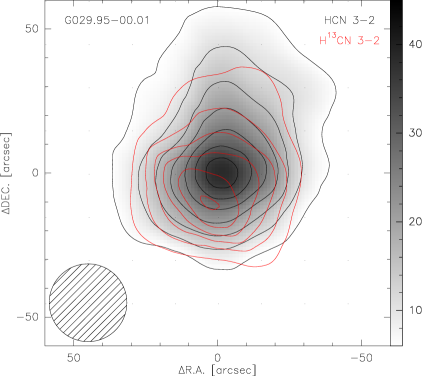
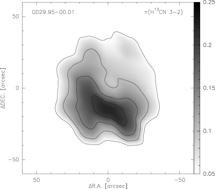
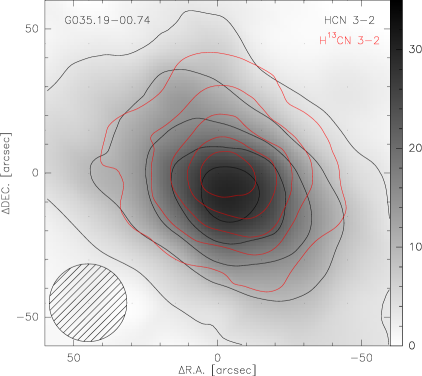
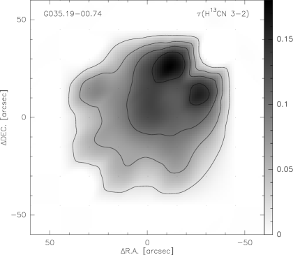
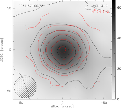
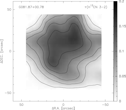
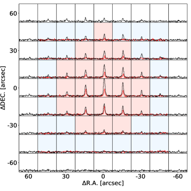
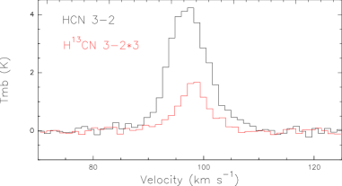
The detailed calculation of the optical depth is described with one source — G029.95-00.01 and one pair of lines — H¹³CN and HCN 3-2 as an example. The velocity integrated intensity map of H¹³CN 3-2 as red contour overlaid on that of HCN 3-2 as grayscale and black contour, is presented in the top left panel of Figure 1. Note that there is an offset of peak position between H¹³CN 3-2 and HCN 3-2. 22 positions with H¹³CN 3-2 emission above 3 $\sigma$ level were selected from this source, which were marked in light pink on the grid-maps for HCN and H¹³CN 3-2 as demonstrated in the top right panel of Figure 1. All the selected spectra of H¹³CN 3-2 were also checked by eye to confirm data quality. The spatial distribution of H¹³CN 3-2 optical depth is presented in the bottom left panel of Figure 1, with contour levels from 0.05 to 0.25. Based on examination of the spectra, the “Spatially resolved” and “Averaged” $\tau$ of H¹³CN 3-2 obtained respectively by two methods were listed in Table 3. $\tau(\textrm{H}^{13}\textrm{CN})$ derived from the spatially resolved information is 0.1158 $\pm$ 0.0002, while the “Averaged” $\tau(\textrm{H}^{13}\textrm{CN})$ is 0.1157 $\pm$ 0.0002. For the 22 positions located at “center” of the core, the intensity flux of H¹³CN is 34.99 $\pm$ 0.86 K km s^-1 and taking 86.4% of the total H¹³CN flux, while the “center” HCN only contains 64.8% flux within the 2 ${}^{\prime}\times 2^{\prime}$ region. The uncertainty of “Averaged” $\tau(\textrm{H}^{13}\textrm{CN})$ is calculated from the intensity flux error propagation, while the same value is adopted as uncertainty of the “Spatially resolved” $\tau(\textrm{H}^{13}\textrm{CN})$ . For the region with detectable emission above 3 $\sigma$ level of H¹³CN 3-2, $\tau$ derived from the two methods for G029.95-00.01 are generally agreed well with each other.

Meanwhile, we also obtained the averaged $\tau(\textrm{H}^{13}\textrm{CN})$ for the positions with H¹³CN 3-2 data included in 1.5 ${}^{\prime}\times 1.5^{\prime}$ mapping area, but the intensities of which are less than 3 ${\sigma}$ level and not used for calculation of the spatially resolved $\tau(\textrm{H}^{13}\textrm{CN})$ . Since the re-grid step is 15^′′, there are $7\times 7=49$ positions in total within1.5 ${}^{\prime}\times 1.5^{\prime}$ isotopologue mapping area. Besides the selected 22 positions out of 49 worked for $\tau$ examination by two methods, there are 27 positions left, which are marked in light blue with the same area on grid-maps of HCN 3-2 and H¹³CN 3-2 in Figure 1 and labeled as “middle” part.

Even though no significant signal of individual H¹³CN 3-2 emission in these 27 positions, the averaged or stacked spectrum of H¹³CN 3-2 do have about 5 $\sigma$ detection. We obtained $\tau$ by using Method 2 for the 27 positions without significant signal of H¹³CN 3-2 emission. The result is shown in Table 3 and marked as “Averaged (middle). The $\tau(\textrm{H}^{13}\textrm{CN})$ of the 27 positions is 0.0512 $\pm$ 0.0005, which is about half of $\tau(\textrm{H}^{13}\textrm{CN})$ derived from the area of “center part”.

The intensity flux of H¹³CN and HCN 3-2 for the 27 “middle” positions are 5.5 $\pm$ 1.1 K km s^-1 and 95.6 $\pm$ 3.8 K km s^-1 respectively, taking about 13.6% and 19.5% of the total flux in each case.

Since the HCN 3-2 mapping size is 2 ${}^{\prime}\times 2^{\prime}$ , there are $9\times 9=81$ positions with re-grid step of 15^′′. In fact, there are 32 positions have HCN 3-2 data and without H¹³CN 3-2 data, which are marked as “outside” positions. It is impossible to calculate even for the averaged optical depths of H¹³CN and HCN 3-2 there. However, since H¹³CN 3-2 emission is quickly decreasing from center to the outside and even the “middle” 27 positions only contain $\sim$ 13.6% flux within the 1.5 ${}^{\prime}\times 1.5^{\prime}$ region, we can neglect the contribution of H¹³CN 3-2 emission in “outside” positions when counting total H¹³CN 3-2 flux in this molecular core. But the HCN 3-2 emission can still be detected in such region. The stacked intensity flux of the “outside” for HCN emission is 67.2 $\pm$ 3.9 K km s^-1 and contains 13.7% of the total HCN 3-2 flux. The contribution of the outside HCN 3-2 emission is listed in Table 3 and marked as “Averaged (outside)”.

In addition, we also calculated the averaged optical depths of H¹³CN and HCN 3-2 of this molecular core, which derived from the flux ratio of total H¹³CN emission for 1.5 ${}^{\prime}\times 1.5^{\prime}$ and HCN emission for 2 ${}^{\prime}\times 2^{\prime}$ . The total flux of HCN, obtained by averaged spectrum in the 2 ${}^{\prime}\times 2^{\prime}$ regions, is 490.1 $\pm$ 6.1 K km s^-1, approximately equals to the sum of flux from “center”, “middle” and “outside” parts. Also, the total flux of H¹³CN as 40.5 $\pm$ 1.6 K km s^-1 is similar to the sum of fluxes from “center” and “middle”. By taking the H¹³CN/HCN 3-2 ratio as 0.0826 $\pm$ 0.0023 and using Method 2, we obtained the $\tau(\textrm{H}^{13}\textrm{CN})$ as 0.0832 $\pm$ 0.0003, which was moderately lower than that from the “center” part. The results are listed in Table 3 and marked as “Averaged (whole)”. For a short summary of the optical depths obtained in different regions, including “center”, “middle” and “outside” parts, the derived values are decreasing from center to the outside. The results of “middle” and “outside” parts are just for showing the optical depth distribution in individual sources itself, which will not be used for the discussions in next section.

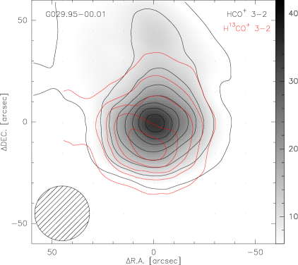
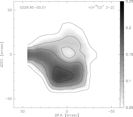
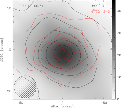
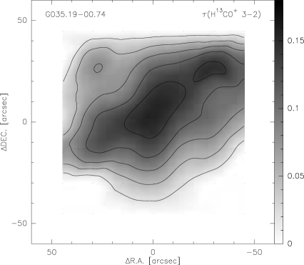
For another pair of lines — HCO $+$ and H¹³CO⁺, the same procedures are adopted for the optical depths calculation in different conditions, respectively. The results are listed in Table 4.

Table 3: Optical depth derived from HCN 3-2 of G029.95-00.01.

Range	$I(\textrm{HCN})$	$I(\textrm{H}^{13}\textrm{CN})$	$I(\textrm{H}^{13}\textrm{CN})/I(\textrm{HCN})$	$\tau(\textrm{H}^{13}\textrm{CN})$	$\tau(\textrm{HCN})$
	K km s^-1	K km s^-1
Spatially resolved (22, HCN weighted)				0.1158 $\pm$ 0.0002	4.633 $\pm$ 0.008
Averaged (center, 22)	317.4 $\pm$ 2.8	34.99 $\pm$ 0.86	0.1102 $\pm$ 0.0015	0.1157 $\pm$ 0.0002	4.628 $\pm$ 0.008
Averaged (middle, 27)	95.6 $\pm$ 3.8	5.5 $\pm$ 1.1	0.0571 $\pm$ 0.0094	0.0512 $\pm$ 0.0005	2.048 $\pm$ 0.020
Averaged (outside, 32)	67.2 $\pm$ 3.9	—	—	—	—
Averaged (whole)	490.1 $\pm$ 6.1	40.5 $\pm$ 1.6	0.0826 $\pm$ 0.0023	0.0832 $\pm$ 0.0003	3.328 $\pm$ 0.012

Table 4: Optical depth derived from HCO⁺ 3-2 of G029.95-00.01.

Range	$I(\textrm{HCO}^{+})$	$I(\textrm{H}^{13}\textrm{CO}^{+})$	$I(\textrm{H}^{13}\textrm{CO}^{+})/I(\textrm{HCO}^{+})$	$\tau(\textrm{H}^{13}\textrm{CO}^{+})$	$\tau(\textrm{HCO}^{+})$
	K km s^-1	K km s^-1
Spatially resolved (19, HCO⁺ weighted)				0.1069 $\pm$ 0.0001	4.276 $\pm$ 0.004
Averaged (center, 19)	240.3 $\pm$ 2.0	24.74 $\pm$ 0.43	0.1030 $\pm$ 0.0009	0.1073 $\pm$ 0.0001	4.292 $\pm$ 0.004
Averaged (middle, 30)	137.4 $\pm$ 2.8	6.36 $\pm$ 0.61	0.0463 $\pm$ 0.0035	0.0367 $\pm$ 0.0001	1.468 $\pm$ 0.004
Averaged (outside, 32)	98.6 $\pm$ 2.8	—	—	—	—
Averaged (whole)	476.3 $\pm$ 5.2	31.12 $\pm$ 0.68	0.0653 $\pm$ 0.0007	0.0619 $\pm$ 0.0001	2.476 $\pm$ 0.004

Table 5: Optical depths of H¹³CN 3-2 and H¹³CO⁺ 3-2 for 30 sources.

	$\tau(\textrm{H}^{13}\textrm{CN})$					$\tau(\textrm{H}^{13}\textrm{CO}^{+})$
Source name	Pts^†	Spatially resolved	Ave (center)	Ave (whole)	Ave (middle)	Pts^†	Spatially resolved	Ave (center)	Ave (whole)	Ave (middle)
G005.88-00.39	20	0.1523 $\pm$ 0.0002	0.1515 $\pm$ 0.0002	0.1187 $\pm$ 0.0005	0.0398 $\pm$ 0.0002	28	0.1062 $\pm$ 0.0001	0.1065 $\pm$ 0.0001	0.0951 $\pm$ 0.0002	0.0626 $\pm$ 0.0005
G009.62+00.19	12	0.1654 $\pm$ 0.0006	0.1652 $\pm$ 0.0005	0.1143 $\pm$ 0.0010	0.0748 $\pm$ 0.0015	15	0.1114 $\pm$ 0.0003	0.1115 $\pm$ 0.0003	0.0722 $\pm$ 0.0006	0.0492 $\pm$ 0.0002
G010.47+00.02	18	0.1663 $\pm$ 0.0005	0.1652 $\pm$ 0.0005	0.1242 $\pm$ 0.0012	0.0809 $\pm$ 0.0015	14	0.1055 $\pm$ 0.0005	0.1057 $\pm$ 0.0005	0.0771 $\pm$ 0.0006	0.0748 $\pm$ 0.0009
G010.62-00.38	31	0.1535 $\pm$ 0.0001	0.1534 $\pm$ 0.0001	0.1282 $\pm$ 0.0002	0.0714 $\pm$ 0.0004	30	0.1686 $\pm$ 0.0001	0.1679 $\pm$ 0.0001	0.1359 $\pm$ 0.0001	0.0527 $\pm$ 0.0006
G011.49-01.48	12	0.0771 $\pm$ 0.0001	0.0775 $\pm$ 0.0001	0.0336 $\pm$ 0.0002	—	22	0.0717 $\pm$ 0.0001	0.0718 $\pm$ 0.0001	0.0542 $\pm$ 0.0003	0.0398 $\pm$ 0.0004
G011.91-00.61	13	0.1139 $\pm$ 0.0003	0.1141 $\pm$ 0.0003	0.0912 $\pm$ 0.0003	0.0352 $\pm$ 0.0004	15	0.1078 $\pm$ 0.0005	0.1080 $\pm$ 0.0005	0.0920 $\pm$ 0.0004	0.0405 $\pm$ 0.0003
G012.80-00.20	46	0.1026 $\pm$ 0.0001	0.1035 $\pm$ 0.0001	0.0722 $\pm$ 0.0001	0.0478 $\pm$ 0.0006	48	0.1382 $\pm$ 0.0001	0.1380 $\pm$ 0.0001	0.1027 $\pm$ 0.0001	$<$ 0.0764
G014.33-00.64	12	0.1180 $\pm$ 0.0004	0.1179 $\pm$ 0.0004	0.0863 $\pm$ 0.0006	0.0665 $\pm$ 0.0009	25	0.1278 $\pm$ 0.0002	0.1279 $\pm$ 0.0002	0.0806 $\pm$ 0.0001	0.0455 $\pm$ 0.0003
G015.03-00.67	28	0.0733 $\pm$ 0.0001	0.0741 $\pm$ 0.0001	0.0756 $\pm$ 0.0001	0.0962 $\pm$ 0.0002	34	0.1225 $\pm$ 0.0001	0.1225 $\pm$ 0.0001	0.1221 $\pm$ 0.0001	0.1019 $\pm$ 0.0004
G016.58-00.05	11	0.1120 $\pm$ 0.0003	0.1122 $\pm$ 0.0003	0.0890 $\pm$ 0.0011	0.0825 $\pm$ 0.0016	9	0.1129 $\pm$ 0.0003	0.1128 $\pm$ 0.0003	0.0790 $\pm$ 0.0011	0.0672 $\pm$ 0.0011
G023.00-00.41	11	0.1630 $\pm$ 0.0006	0.1614 $\pm$ 0.0006	0.0939 $\pm$ 0.0009	0.0699 $\pm$ 0.0011	14	0.0905 $\pm$ 0.0002	0.0912 $\pm$ 0.0002	0.0409 $\pm$ 0.0002	0.0176 $\pm$ 0.0001
G027.36-00.16	12	0.0867 $\pm$ 0.0002	0.0870 $\pm$ 0.0002	0.0855 $\pm$ 0.0008	0.0661 $\pm$ 0.0018	21	0.1008 $\pm$ 0.0002	0.1012 $\pm$ 0.0002	0.0909 $\pm$ 0.0006	0.0600 $\pm$ 0.0013
G029.95-00.01	22	0.1158 $\pm$ 0.0002	0.1157 $\pm$ 0.0002	0.0832 $\pm$ 0.0003	0.0512 $\pm$ 0.0005	19	0.1069 $\pm$ 0.0001	0.1073 $\pm$ 0.0001	0.0619 $\pm$ 0.0001	0.0367 $\pm$ 0.0001
G035.02+00.34	10	0.1120 $\pm$ 0.0003	0.1214 $\pm$ 0.0003	0.0768 $\pm$ 0.0009	0.0348 $\pm$ 0.0006	11	0.1126 $\pm$ 0.0005	0.1237 $\pm$ 0.0005	0.1008 $\pm$ 0.0014	0.1088 $\pm$ 0.0024
G035.19-00.74	22	0.0828 $\pm$ 0.0002	0.0851 $\pm$ 0.0002	0.0638 $\pm$ 0.0003	0.0550 $\pm$ 0.0004	29	0.0975 $\pm$ 0.0002	0.0985 $\pm$ 0.0002	0.0645 $\pm$ 0.0003	0.0260 $\pm$ 0.0002
G037.43+01.51	10	0.0966 $\pm$ 0.0004	0.0970 $\pm$ 0.0004	0.0722 $\pm$ 0.0006	0.0508 $\pm$ 0.0007	20	0.0815 $\pm$ 0.0001	0.0825 $\pm$ 0.0001	0.0626 $\pm$ 0.0002	0.0298 $\pm$ 0.0004
G043.16+00.01	30	0.0979 $\pm$ 0.0001	0.0989 $\pm$ 0.0001	0.0680 $\pm$ 0.0001	0.0295 $\pm$ 0.0002	34	0.0883 $\pm$ 0.0001	0.0893 $\pm$ 0.0001	0.0645 $\pm$ 0.0001	—
G043.79-00.12	8	0.1008 $\pm$ 0.0004	0.1015 $\pm$ 0.0004	0.0939 $\pm$ 0.0011	0.0922 $\pm$ 0.0024	8	0.0820 $\pm$ 0.0002	0.0829 $\pm$ 0.0002	0.0573 $\pm$ 0.0005	0.0188 $\pm$ 0.0003
G049.48-00.36	36	0.1105 $\pm$ 0.0001	0.1107 $\pm$ 0.0001	0.0764 $\pm$ 0.0001	0.0123 $\pm$ 0.0001	41	0.1092 $\pm$ 0.0001	0.1096 $\pm$ 0.0001	0.0745 $\pm$ 0.0001	0.0321 $\pm$ 0.0003
G049.48-00.38	32	0.1573 $\pm$ 0.0002	0.1557 $\pm$ 0.0002	0.1134 $\pm$ 0.0002	0.0619 $\pm$ 0.0003	34	0.1259 $\pm$ 0.0002	0.1258 $\pm$ 0.0002	0.0897 $\pm$ 0.0002	0.0180 $\pm$ 0.0001
G069.54-00.97	19	0.1257 $\pm$ 0.0007	0.1252 $\pm$ 0.0007	0.0864 $\pm$ 0.0012	0.0199 $\pm$ 0.0005	33	0.1019 $\pm$ 0.0001	0.1035 $\pm$ 0.0001	0.0748 $\pm$ 0.0001	0.0348 $\pm$ 0.0004
G075.76+00.33	21	0.0408 $\pm$ 0.0001	0.0413 $\pm$ 0.0001	0.0214 $\pm$ 0.0001	0.0165 $\pm$ 0.0001	17	0.0387 $\pm$ 0.0001	0.0398 $\pm$ 0.0001	0.0192 $\pm$ 0.0001	0.0260 $\pm$ 0.0001
G078.12+03.63	9	0.0473 $\pm$ 0.0001	0.0478 $\pm$ 0.0001	0.0180 $\pm$ 0.0001	—	23	0.0876 $\pm$ 0.0002	0.0886 $\pm$ 0.0002	0.0748 $\pm$ 0.0003	0.0493 $\pm$ 0.0005
G081.87+00.78	34	0.0972 $\pm$ 0.0001	0.0983 $\pm$ 0.0001	0.0672 $\pm$ 0.0001	—	44	0.0884 $\pm$ 0.0001	0.0893 $\pm$ 0.0001	0.0706 $\pm$ 0.0001	0.0188 $\pm$ 0.0001
G109.87+02.11	32	0.0747 $\pm$ 0.0001	0.0764 $\pm$ 0.0001	0.0520 $\pm$ 0.0001	0.0199 $\pm$ 0.0001	47	0.1008 $\pm$ 0.0001	0.1012 $\pm$ 0.0001	0.0775 $\pm$ 0.0001	0.0535 $\pm$ 0.0011
G121.29+00.65	16	0.0735 $\pm$ 0.0002	0.0741 $\pm$ 0.0002	0.0462 $\pm$ 0.0003	0.0375 $\pm$ 0.0003	20	0.0829 $\pm$ 0.0001	0.0840 $\pm$ 0.0001	0.0504 $\pm$ 0.0002	0.0283 $\pm$ 0.0002
G123.06-06.30	9	0.1008 $\pm$ 0.0004	0.1008 $\pm$ 0.0004	0.0718 $\pm$ 0.0008	0.0451 $\pm$ 0.0007	17	0.0640 $\pm$ 0.0001	0.0645 $\pm$ 0.0001	0.0470 $\pm$ 0.0002	0.0584 $\pm$ 0.0010
G133.94+01.06	26	0.1184 $\pm$ 0.0002	0.1195 $\pm$ 0.0002	0.0909 $\pm$ 0.0002	0.0733 $\pm$ 0.0003	34	0.0845 $\pm$ 0.0001	0.0855 $\pm$ 0.0001	0.0672 $\pm$ 0.0001	0.0352 $\pm$ 0.0001
G188.94+00.88	10	0.0544 $\pm$ 0.0002	0.0550 $\pm$ 0.0002	—	—	26	0.0531 $\pm$ 0.0001	0.0542 $\pm$ 0.0001	0.0367 $\pm$ 0.0001	—
G232.62+00.99	6	0.0820 $\pm$ 0.0008	0.0825 $\pm$ 0.0008	0.0839 $\pm$ 0.0024	0.0947 $\pm$ 0.0023	17	0.0912 $\pm$ 0.0004	0.0920 $\pm$ 0.0004	0.0825 $\pm$ 0.0006	0.0733 $\pm$ 0.0007

^† Number of positions adopted for the calculation of spatially resolved optical depth.

4 Results

Following methods described in §3, the parameters of two pairs of dense gas tracers of 30 clouds are derived and listed in Table LABEL:tab:tau-all. Only optical depths of H¹³CN 3-2 and H¹³CO⁺ 3-2 are listed, while HCN 3-2 and HCO⁺ 3-2 informations are not included, since they can be simply obtained by multiplying by 40 based on the assumption. However, the abundance ratio of ¹²C/¹³C can vary from less than 40 to be even close to 100 (Wilson & Rood, 1994; Milam et al., 2005). Since HCN 3-2 and HCO⁺ 3-2 are mainly optically thick, the derived optical depths of H¹³CN 3-2 and H¹³CO⁺ 3-2 are almost not related to the assumed abundance ratio, except for some sources with line ratios of HCN/H¹³CN 3-2 or HCO⁺/H¹³CO⁺ 3-2 close to 40. In the extreme cases with the line ratios greater than 40, there will be no solution for optical depths under such assumption, which are listed as ‘ $-$ ’ for out regions of several sources in Table LABEL:tab:tau-all. Note that the “Spatially resolved” and “Averaged (center)” ones, which are used for the scientific discussions in next section, do have solution for all sources. Consequently, the derived optical depths of H¹³CN 3-2 and H¹³CO⁺ 3-2 are reliable, even if the assumption of abundance ratio is not accurate. Since the assumed abundance ratio will only strongly affect the absolute optical depths of HCN 3-2 and HCO⁺ 3-2 in each source, while we are focusing on the relative different between the optical depths of H¹³CN 3-2 and H¹³CO⁺ 3-2 derived with two methods, we do not use different assumed abundance ratio in each source.

Column 2 – 5 in Table LABEL:tab:tau-all contain information on $\tau(\textrm{H}^{13}\textrm{CN})$ , which are the numbers of positions selected for the spatially resolved $\tau(\textrm{H}^{13}\textrm{CN})$ , the $\tau(\textrm{H}^{13}\textrm{CN})$ values of “spatially resolved”, and the “Averaged (center)”, “Averaged (whole)”, “Averaged (middle)” , respectively. While the column 6 – 10 represent the the numbers of positions selected for the spatially resolved $\tau(\textrm{H}^{13}\textrm{CO}^{+})$ and the four kinds of $\tau(\textrm{H}^{13}\textrm{CO}^{+})$ . Note that “Averaged (whole)” $\tau(\textrm{H}^{13}\textrm{CN})$ in G188.94+00.88, “Averaged (middle)” $\tau(\textrm{H}^{13}\textrm{CN})$ in G011.49-01.48, G078.12+03.63, G081.87+00.78, and G188.94+00.88, and “Averaged (middle)” $\tau(\textrm{H}^{13}\textrm{CO}^{+})$ in G043.16+00.01 and G188.94+00.88, are marked as ‘ $-$ ’, with no solutions caused by high line ratio of HCN/H¹³CN 3-2 or HCO⁺/H¹³CO⁺ 3-2, which are described before. Since there is only one point left for the calculation of “Averaged (middle)” $\tau(\textrm{H}^{13}\textrm{CO}^{+})$ in G12.80-00.20, only upper limit is obtained. We checked other sources with data points used for calculating $\tau(\textrm{H}^{13}\textrm{CN})$ or $\tau(\textrm{H}^{13}\textrm{CO}^{+})$ larger than 35, which means that only several data points are used to derive “Averaged (middle)” optical depths. All sources do have H¹³CN or H¹³CO⁺ 3-2 signals after averaging the spectra. Special notes need to be mentioned for G049.48-00.36 and G049.48-00.38, which are very close to each other and contaminate the outside regions each other. Therefore, the data points used for “Averaged (middle)” are less than 49 subtracted by that used in “Averaged (middle)”. Also, the value of “Averaged (whole)” in these two sources can also be over-estimated.

With the data points located in same region, $\tau(\textrm{H}^{13}\textrm{CN})$ (or $\tau(\textrm{H}^{13}\textrm{CO}^{+})$ ) derived from the two different methods described in §3, i. e. the “Spatially resolved” and “Averaged (center)” $\tau(\textrm{H}^{13}\textrm{CN})$ (or $\tau(\textrm{H}^{13}\textrm{CO}^{+})$ ), are generally consistent with each other. Besides, both the “Averaged (whole)” $\tau(\textrm{H}^{13}\textrm{CN})$ and $\tau(\textrm{H}^{13}\textrm{CO}^{+})$ are significantly smaller than those $\tau^{13}$ of the “spatially resolved” or “Averaged (center)”. The reason is that the optical depths calculated by “Averaged (whole)” contains more outer points where have no detectable H¹³CN or H¹³CO⁺ 3-2 emission.

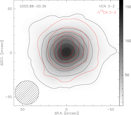
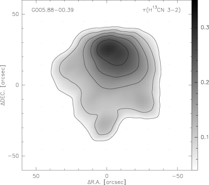
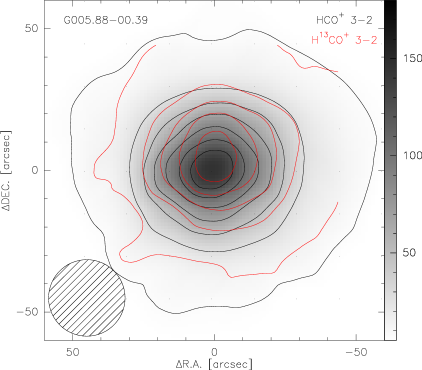
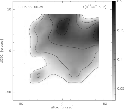
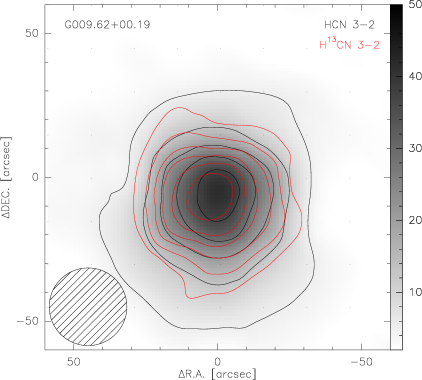
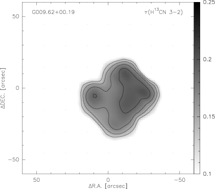
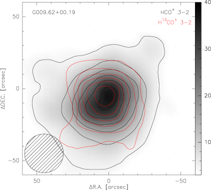
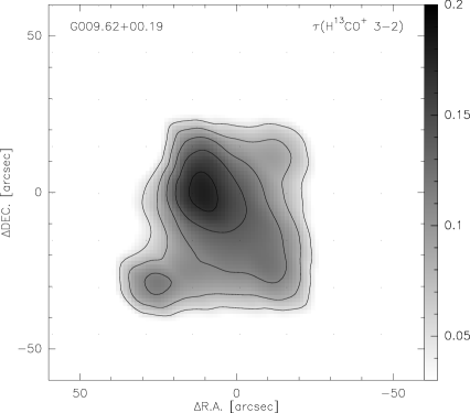
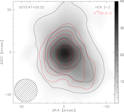
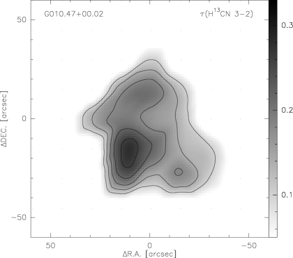
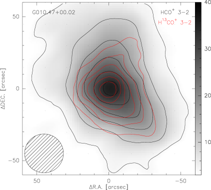
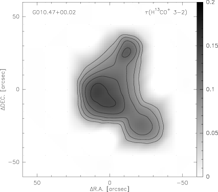
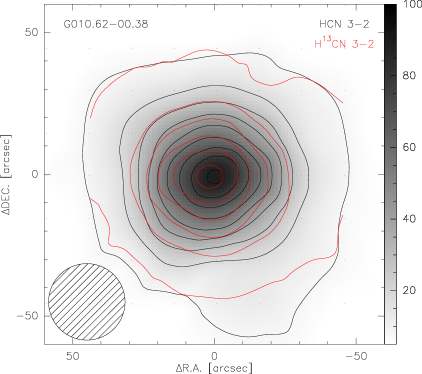
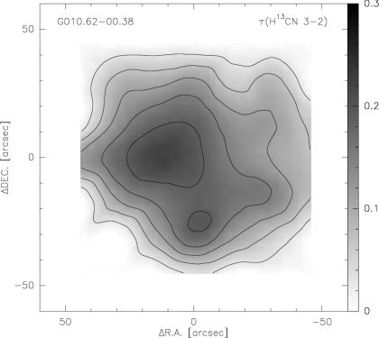
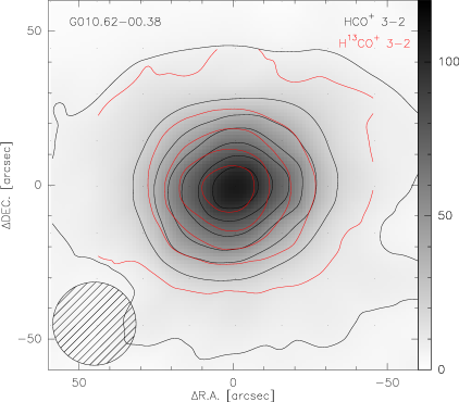
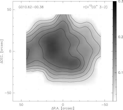
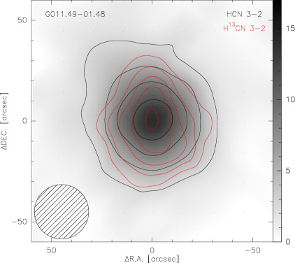
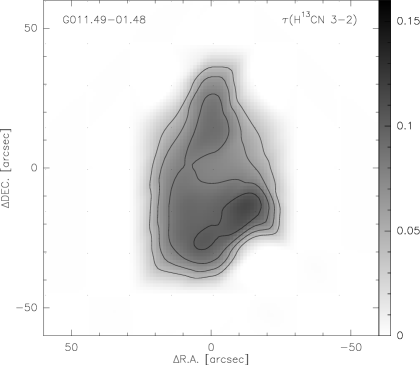
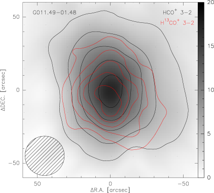
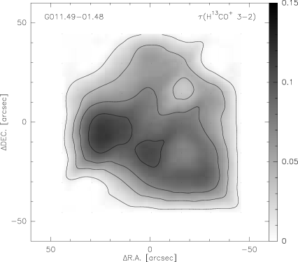
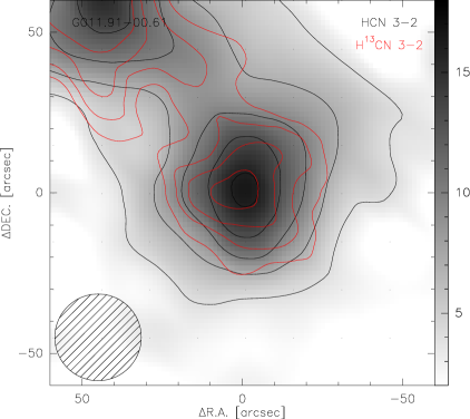
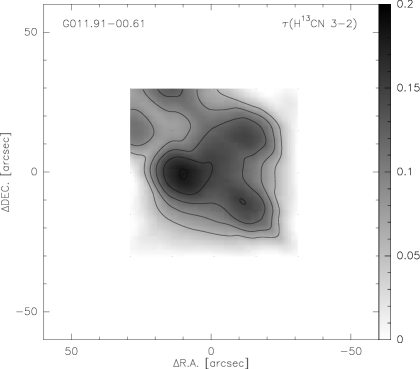
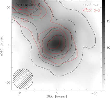
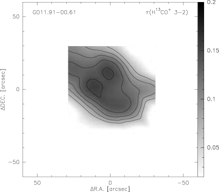
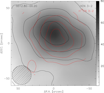
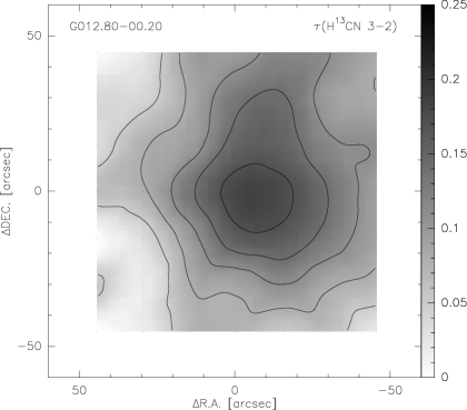
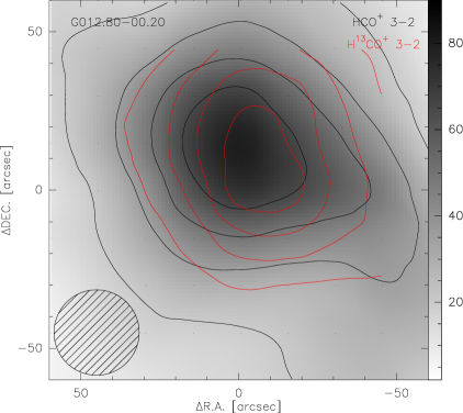
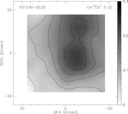
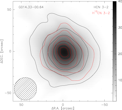
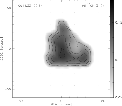
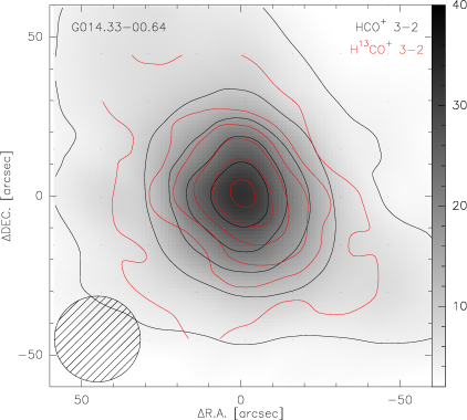
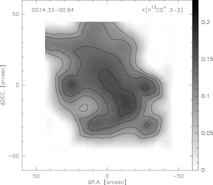
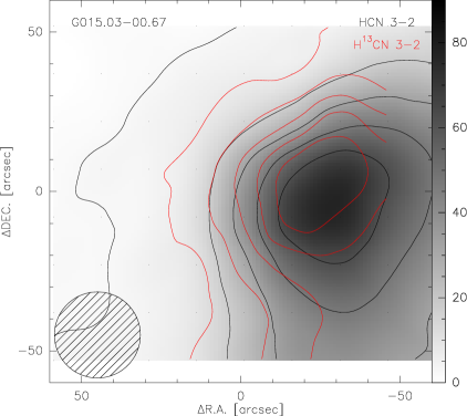
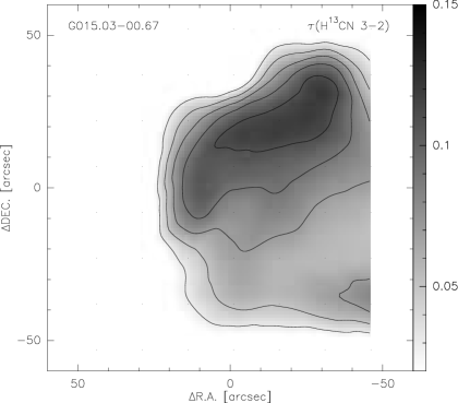
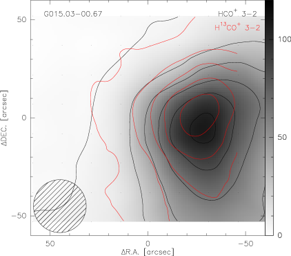
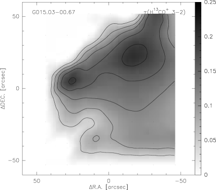
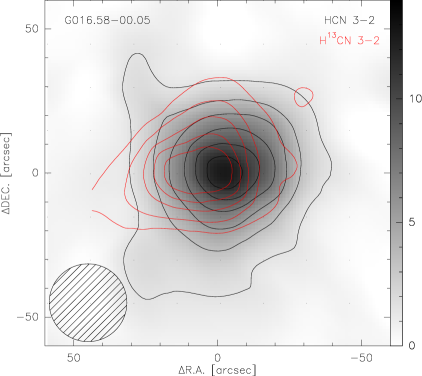
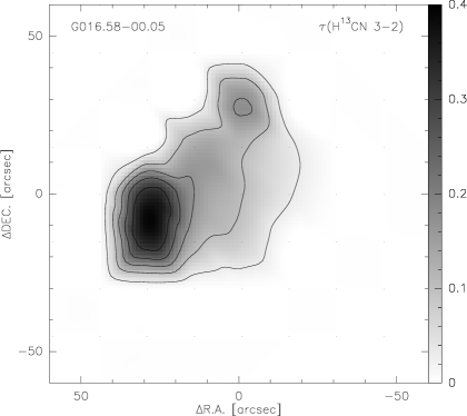
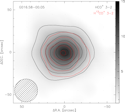
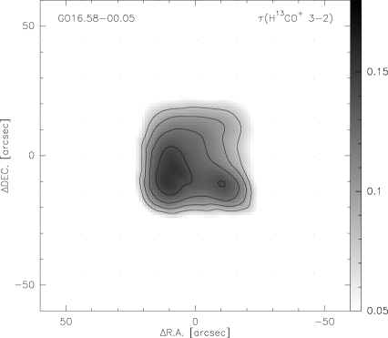
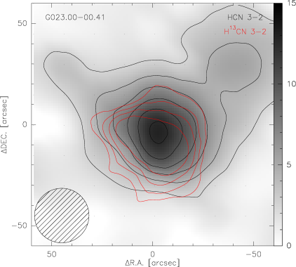
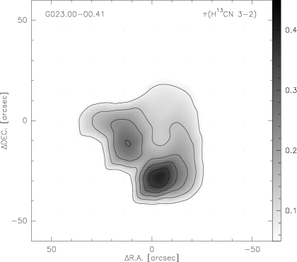
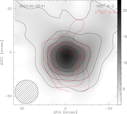
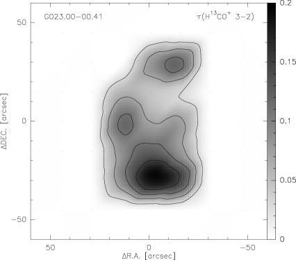
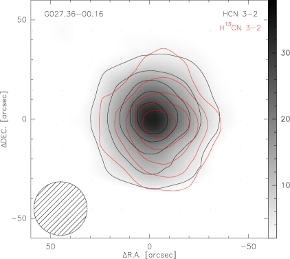
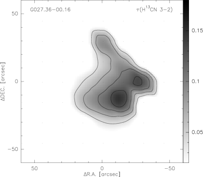
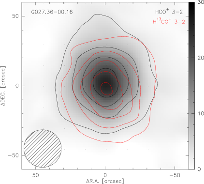
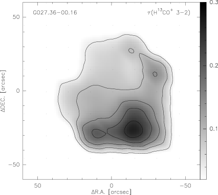
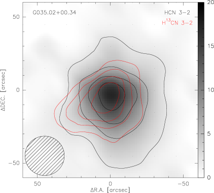
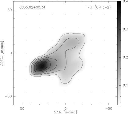
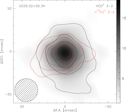
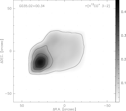
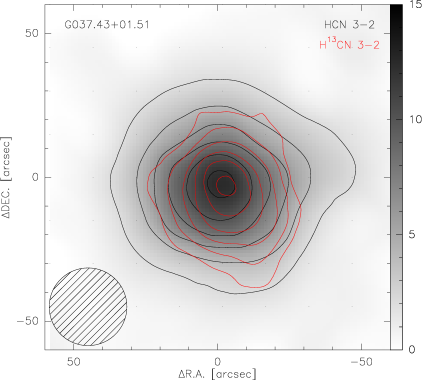
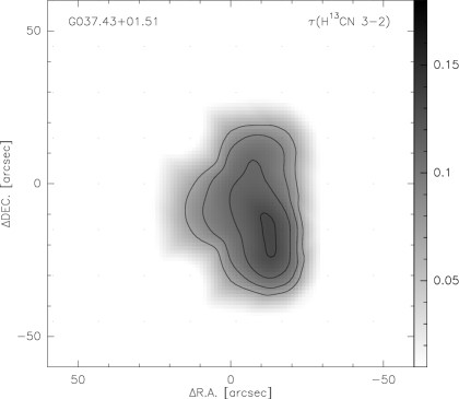
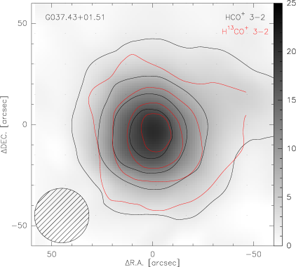
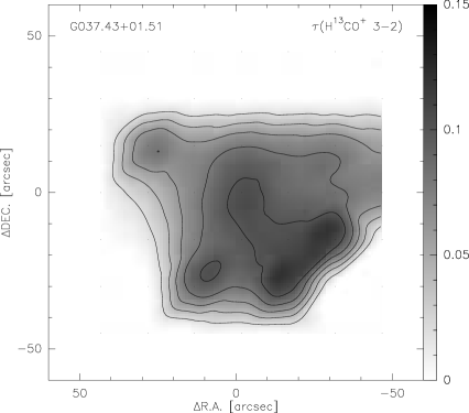
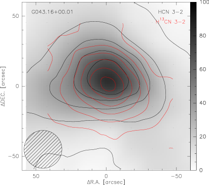
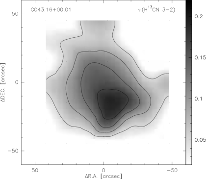
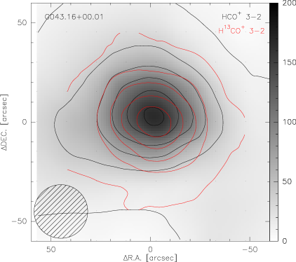
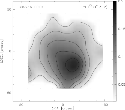
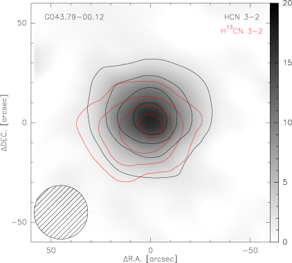
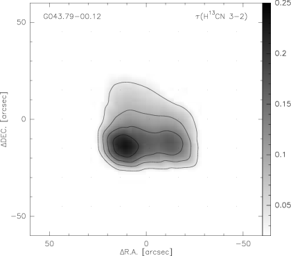
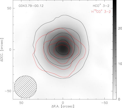
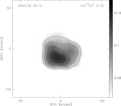
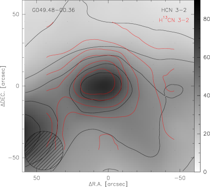
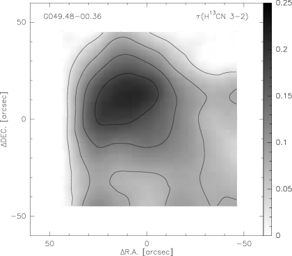
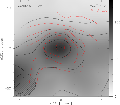
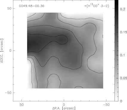
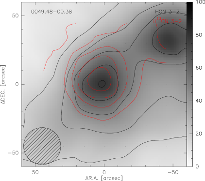
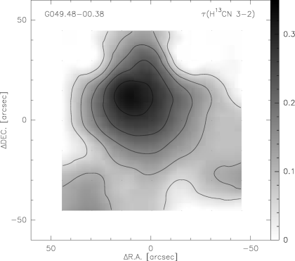
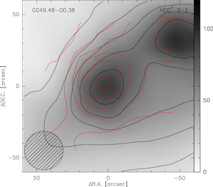
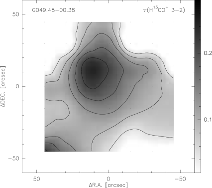
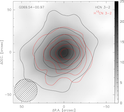
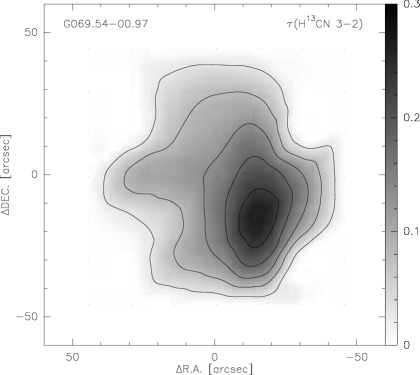
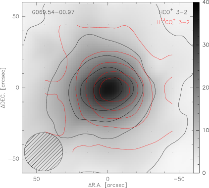
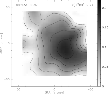
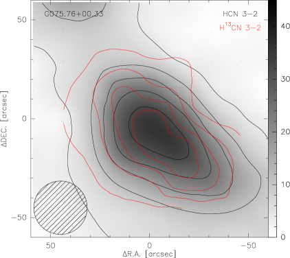
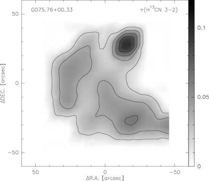
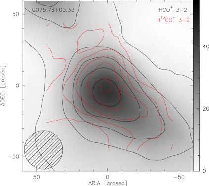
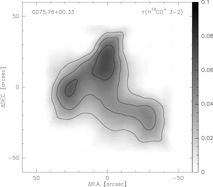
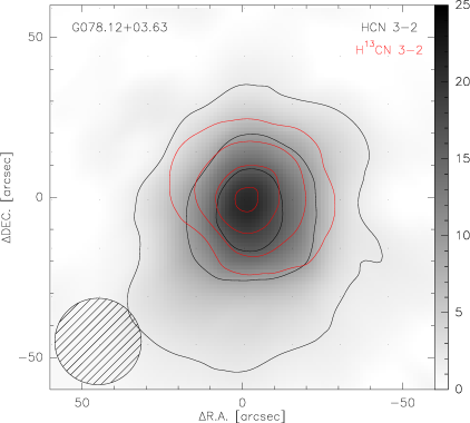
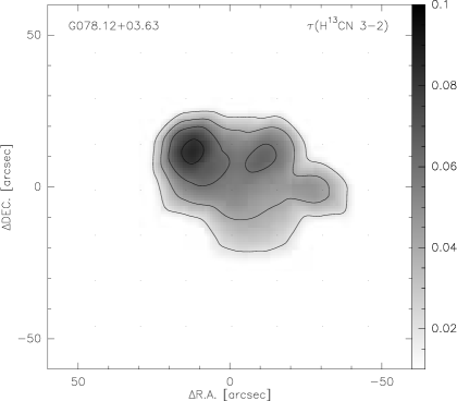
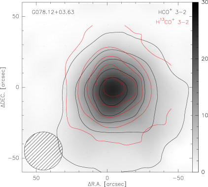
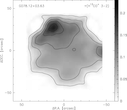
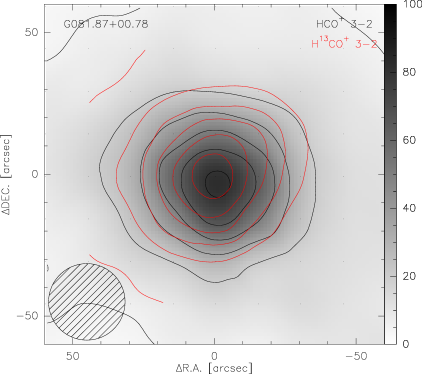
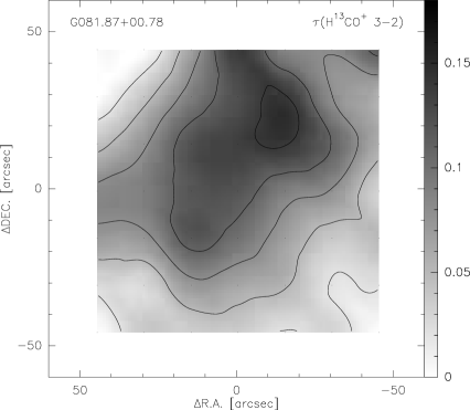
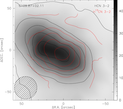
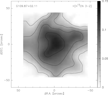
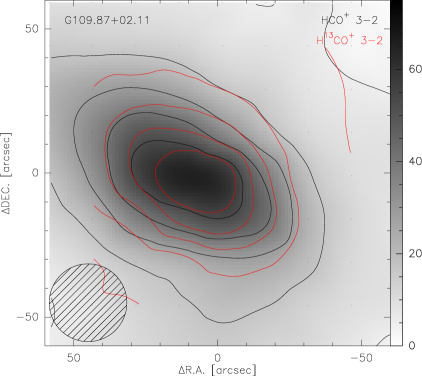
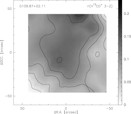
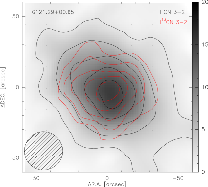
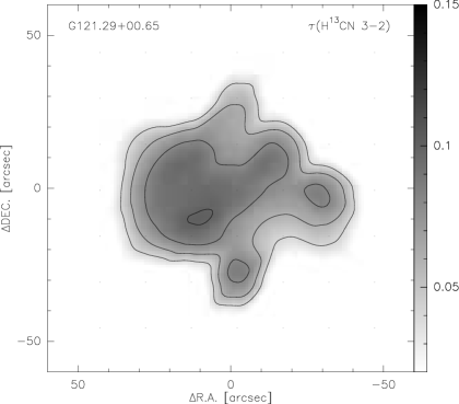
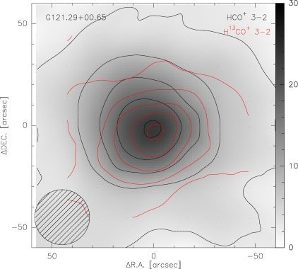
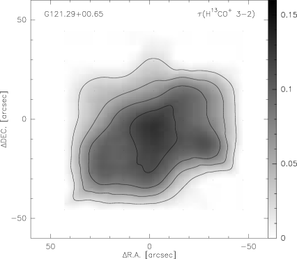
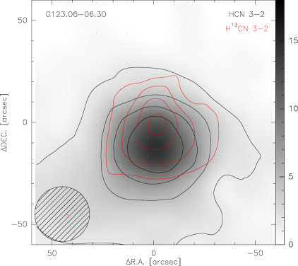
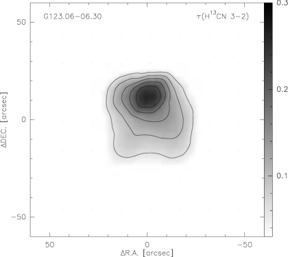
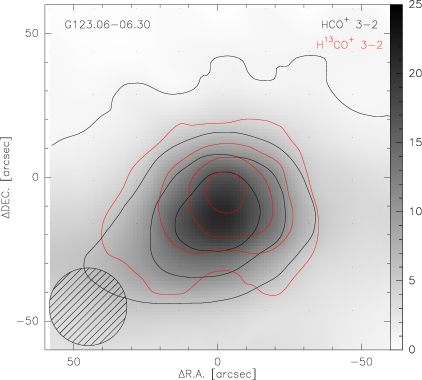
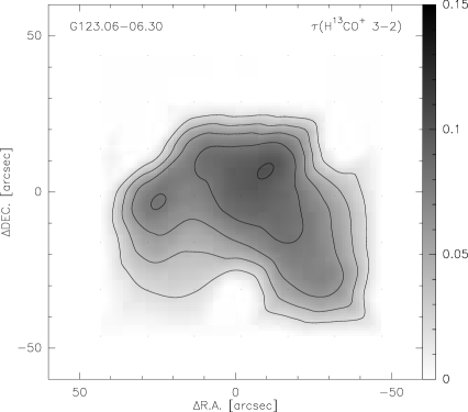
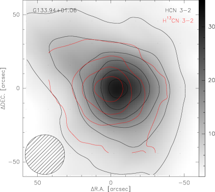
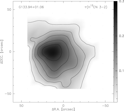
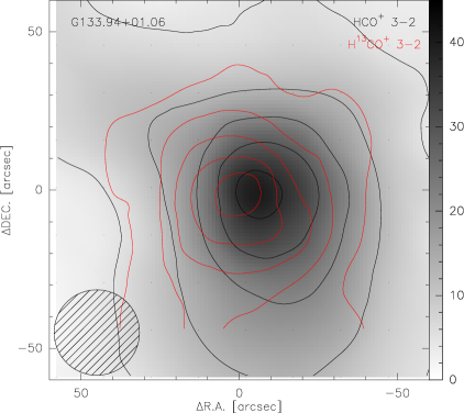
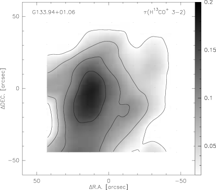
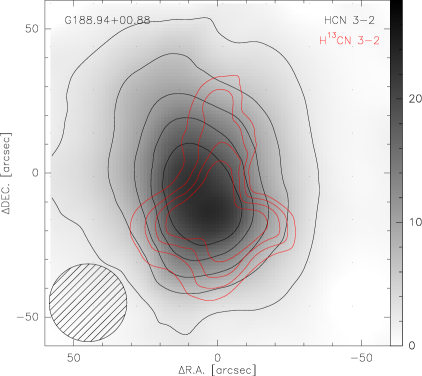
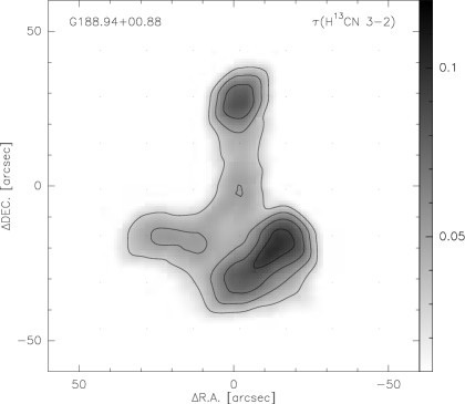
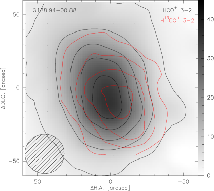
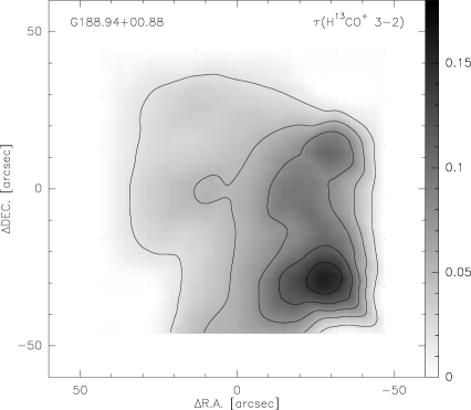
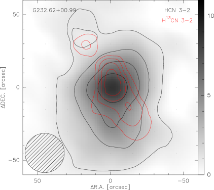
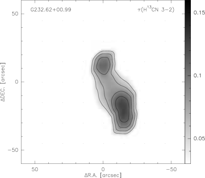
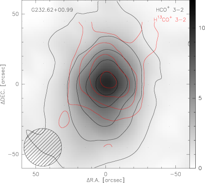
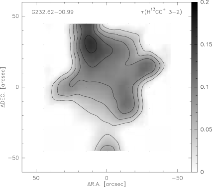
The velocity integrated intensity maps of two pairs of lines, as well as the spatially resolved $\tau$ of H¹³CN 3-2 and H¹³CO⁺ 3-2 of the 30 sources are also presented in Appendix A.

5 Discussion

5.1 The consistency of optical depths derived with two different methods

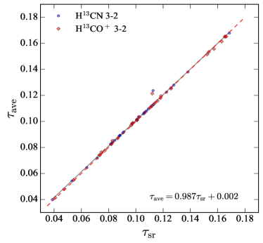
The key question for this paper is to test whether the optical depths calculated with two methods described in §3 are consistent with each other or not. With the information in Table LABEL:tab:tau-all, optical depths of H¹³CN 3-2 derived with the two different methods agree well with each other, within the range from $\sim$ 0.04 in G75.76+00.33 to $\sim$ 0.17 in G010.47+00.02 and G010.62-00.38, with dynamical range of more than 4. The results of the relation between the optical depths derived with two methods for H¹³CO⁺ 3-2 are similar to that of H¹³CN 3-2, while the optical depths of H¹³CN 3-2 and H¹³CO⁺ 3-2 in each source do not show strong correlation, with correlation coefficient of 0.549. The plot for optical depths of H¹³CN and H¹³CO⁺ 3-2 derived with these methods are presented in Figure 2, where H¹³CN and H¹³CO⁺ 3-2 in one source are considered as two independent data points. The dashed red line is a simple function of “y=x”, while the black line is the linear least-square fitting result of “y=0.987x+0.002” with correlation coefficient of 0.997, which is close to that of “y=x”. Thus, optical depths for such lines of dense cores, derived from integrated flux ratios of dense gas tracers and their isotopologues at different positions, can generally represent the typical optical depths of these sources, without necessary systematic corrections. For Galactic dense cores without spatial resolved information, typical optical depths of those core derived from line ratios of dense gas tracers and their isotopic lines are acceptable, especially for global properties of large sample surveys. Previous studies with dense gas tracers such as CO, HCN, HCO⁺ and HNC and their isotopic lines in a small number of bright galaxies (Nguyen, et al., 1992; Costagliola et al., 2011; Jiang, Wang, & Gu, 2011; Wang et al., 2014, 2016; Li, et al., 2020; Jiménez-Donaire et al., 2017a), the optical depths derived without spatially resolved data, which is similar to method 2, can be considered as a good approximation. Based on our results (see Table 3 and Table LABEL:tab:tau-all), the differences of derived optical depths with the two methods were within 3%, while the uncertainties of isotopic abundance ratio and measured line fluxes in galaxies are normally larger than 10%. Thus, the assumption of isotopic abundance ratio and the measurements of lines can cause larger uncertainties than that caused by the simple assumption of uniform optical depth in different regions.

However, even the optical depths obtained with two methods generally agree well with each other, there can be up to 8% differences to each other in a few sources, such as H¹³CN 3-2 in G035.02+00.34. So for galaxies without spatial resolved line ratio of dense gas tracers and their isotopologues, the accuracy with such simple assumption should be tested with spatially resolved observations for several local galaxies, such as Arp 220, M82, and NGC 253. CN 1-0 and ¹³CN 1-0 observations toward nuclear regions of three nearby galaxies, NGC 253, NGC 1068, and NGC 4945, with ALMA were done recently (Tang et al., 2019), which mainly focused on the ¹²C/¹³C ratio instead of optical depth distribution.

The re-grid steps of the observations are 15^′′, while the FWHM of beamsize is about 27.8^′′. On the other words, the final maps are over-sampled, which means the emission obtained in a certain position is not independent with neighboring positions. Especially, emission can be seen toward several positions even for a point source, with the same line profile. However, normally only 5 positions with offsets (-15^′′, 0^′′), (0^′′, -15^′′), (0^′′, 0^′′), (0^′′, 15^′′) and (15^′′, 0^′′), can have detectable lines. Based on the information listed in Table LABEL:tab:tau-all, no source can be treated as point source. The spatially integrated fluxes of the lines listed in Table 3 need to be corrected by the fraction of sampling size and beamsize. However, the absolute line fluxes are not used for any scientific discussion, while only line ratios are used.

5.2 Assumptions of deriving optical depths with isotopic line ratios

There are several assumptions during the calculation of line optical depths with isotopic line ratios, some of which are implicit and may not be true, such as uniform optical depth within observing beam, uniform excitation conditions within observing beam, no influence of continuum emission to the line radiative transfer, and the same value of molecular isotopic abundance ratio as that of isotopic ratio.

In fact, due to limited spatial resolution and sensitivity, the spatially resolved optical depths obtained with mapping observations of dense gas tracers and their isotoplogues, are averaged for both of the lines within the telescope beam. Thus, the optical depth distribution has already been smoothed. Sensitive high resolution observations of such line pairs are essential for deriving detailed optical depth distribution. Such methods can also be applied to CO lines and their isotopologues, in Galactic molecular clouds as well as molecular gas in galaxies.

We used the fluxes of HCN and HCO⁺ 3-2 respectively as weights when calculating the averages from spatially resolved optical depths. Since the optically thin isotopic lines can better trace gas mass than optically thick lines, isotopic lines are better choice than the optically thick lines if mass weighted optical depths of molecular gas were expected. However, as a dimensionless number, optical depth is the property of one given line at particular frequency (or velocity), instead of the property for a cloud with given mass. The main purpose of focusing on optical depths is to evaluate the self absorption of optically thick lines. The exact number itself of spatially averaged optical depth for one optically thin line is almost useless. For optically thin case, the important parameters, such as beam averaged column density and gas mass, are only related to the velocity integrated fluxes, excitation conditions (i.e., partition function), etc, while the measured velocity integrated fluxes are affected by excitation temperature, and the combination of optical depth and filling factor. Therefore, it is not necessary to discuss the spatially averaged optical depth for one particular optically thin line. Optical depths of H¹³CN and H¹³CO⁺ 3-2 discussed in this paper are worked for the information of HCN and HCO⁺ 3-2, respectively. With the assumption of HCN/H¹³CN and HCO⁺/H¹³CO⁺ abundance ratio, HCN 3-2 (or HCO⁺ 3-2) optical depths can be simply derived from optical depths of H¹³CN 3-2 (or H¹³CO⁺ 3-2). Thus, the typical optical depths of H¹³CN 3-2 (or H¹³CO⁺ 3-2) from averaging different positions are reflecting those of HCN 3-2 (or HCO⁺ 3-2). For spatially averaged optical depths of HCN 3-2 (or HCO⁺ 3-2), the derived values can be used for the self-absorption property of HCN 3-2 (or HCO⁺ 3-2). For this reason, weighting with HCN 3-2 (or HCO⁺ 3-2) fluxes is the only choice to derive typical optical depths with spatially resolved optical depths. In fact, when the line ratios of a pair of lines, such as HCN/H¹³CN 3-2, are used to derive the beam averaged optical depth, weighting with HCN 3-2 fluxes has been used as an implicit assumption.

5.3 The properties of dense gas tracers in these cores

The dynamical range of H¹³CN and H¹³CO⁺ 3-2 optical depths derived in these cores is from about 0.04 in G075.76+00.33 to about 0.17 in G010.47+00.02 (see Table LABEL:tab:tau-all and Figure 2). The main reason of lack of sources with H¹³CN and H¹³CO⁺ 3-2 optical depths higher than 0.17 is due to the properties of such Galactic massive cores. Sources with high optical depth may exist as late stage compact cores with high column and volume density. On the other hand, the limitation of low optical depth part in our sample is the observational bias, since only sources with observable H¹³CN and H¹³CO⁺ 3-2 emissions are selected. Deep mapping observations toward sources with weak H¹³CN and H¹³CO⁺ 3-2 emissions may extend the low optical depth part. The lowest optical depth of H¹³CN and H¹³CO⁺ 3-2 will be limited by the real isotopic abundance ratio, because the line ratio will be the abundance ratio when the main isotopic line, i.e., HCN and HCO⁺ 3-2, are almost optically thin.

The assumption of same excitation condition of molecules within one beam is always used when adopting line ratio of one pair of isotopic lines, such as HCN/H¹³CN 3-2. However, the gradients of excitation temperatures of molecular lines often exist in dense cores. Line profiles with self absorption features of HCN and HCO⁺ 3-2, are observed in the center of several sources, which can cause over-estimation of optical depth. Nevertheless, since we are focusing on the optical depth derived with two different methods instead of discussing gas properties in this paper, such effect can be ignored.

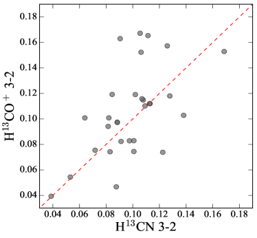
The spatially resolved optical depths of H¹³CN 3-2 and H¹³CO⁺ 3-2 in each source are presented in Figure 3, as $x$ axis and $y$ axis, respectively, with “y = x” as red dash line. With a non-linear coefficient of 0.549, no clear relation between optical depths of H¹³CN 3-2 and H¹³CO⁺ 3-2 can be found. So, even though optical depths of both H¹³CN 3-2 and H¹³CO⁺ 3-2 were used in discussing the difference between two methods, the parameters of H¹³CN 3-2 and H¹³CO⁺ 3-2 in each source are independent, which means that there are 60 data points instead of 30 in Figure 2. The large variation of optical depth ratio between H¹³CN and H¹³CO⁺ 3-2 may be caused by different critical densities as well as possible astrochemical process for HCN and HCO⁺, while ¹²C/¹³C isotopic ratio should not be the reason.

6 Summary and conclusion remarks

With the mapping results of 30 Galactic massive star forming regions for two pairs of lines as HCN and H¹³CN 3-2, as well as HCO⁺ and H¹³CO⁺ 3-2 using the 10-m SMT telescope, we derived optical depths for these sources with two methods to test if the assumption for an uniform optical depth in different positions will strongly affect the typical optical depth in spatially unresolved sources.

The main findings are summarized as follows:

1. Spatially resolved optical depths of H¹³CN and H¹³CO⁺ 3-2 are derived for all 30 sources with the line ratios of HCN/H¹³CN 3-2 and HCO⁺/H¹³CO⁺ 3-2. Significant spatial variation in all sources are found, which indicate that the assumption of uniform optical depth in different positions within one source is incorrect.

2. Based on the spatially resolved optical depths of H¹³CN and H¹³CO⁺ 3-2, we derived the optical depths of H¹³CN 3-2 and H¹³CO⁺ 3-2 for these sources by two ways, the average of spatially resolved $\tau_{sr}$ and the $\tau_{ave}$ from the averaged line ratios, while the latter is widely used in the extragalactic studies. The optical depths obtained with two methods are agree well with each other, from about 0.04 to 0.17, with fitting result of $\tau_{ave}$ =0.987 $\tau_{sr}$ +0.002 and coefficient of 0.997.

3. No clear relation is found for the optical depths of H¹³CN and H¹³CO⁺ 3-2 in the same sources, which means that HCN/HCO⁺ optical depth ratio can vary in different sources caused by chemical and/or physical conditions.

Even though the assumption for an uniform optical depth in different positions of spatially unresolved sources is incorrect, it is a good approximation to derive typical optical depth of molecular lines with isotopic line ratios. Further spatially resolved studies for pair of isotopic lines in galaxies are necessary to do such test.

Acknowledgements

We would like to acknowledge the help of the staff of the SMT 10-m telescope for assistance with the observations. We also acknowledge Li Xiao, Hui Shi and Yan Duan for assisting with the remote observations. We are grateful to the anonymous referee for the constructive report that improved this paper. This work is supported by the National Natural Science Foundation of China grant No. 11988101, 12173067, 12103024, 11725313, 12041302, 12041305, 12173016, 11903003 and the fellowship of China Postdoctoral Science Foundation 2021M691531. Z.-Y Zhang acknowledge the Program for Innovative Talents, Entrepreneur in Jiangsu, acknowledge the science research grants from the China Manned Space Project with NOs.CMS-CSST-2021-A08 and CMS-CSST-2021-A07. N.-Y. Tang is sponsored by Zhejiang Lab Open Research Project (NO. K2022PE0AB01), Cultivation Project for FAST Scientific Payoff and Research Achievement of CAMS-CAS, National key R&D program of China under grant No. 2018YFE0202900 and the University Annual Scientific Research Plan of Anhui Province (NO.2022AH010013).

Data availability

The derived optical depths of H¹³CN and H¹³CO⁺ 3-2 for 30 sources are listed in Table LABEL:tab:tau-all. The data underlying this paper will be shared on a reasonable request to the corresponding authors.

References

Cormier et al. (2018) Cormier D., Bigiel F., Jiménez-Donaire M. J., Leroy A. K., Gallagher M., Usero A., Sandstrom K., et al., 2018, MNRAS, 475, 3909. doi:10.1093/mnras/sty05
Costagliola et al. (2011) Costagliola F., Aalto S., Rodriguez M. I., Muller S., Spoon H. W. W., Martín S., Peréz-Torres M. A., et al., 2011, A&A, 528, A30. doi:10.1051/0004-6361/201015628
den Brok et al. (2022) den Brok J. S., Bigiel F., Sliwa K., Saito T., Usero A., Schinnerer E., Leroy A. K., et al., 2022, A&A, 662, A89. doi:10.1051/0004-6361/202142247
den Brok et al. (2021) den Brok J. S., Chatzigiannakis D., Bigiel F., Puschnig J., Barnes A. T., Leroy A. K., Jiménez-Donaire M. J., et al., 2021, MNRAS, 504, 3221. doi:10.1093/mnras/stab859
Evans (2008) Evans N. J., 2008, ASPC, 390, 52, ASPC..390
Gallagher et al. (2018) Gallagher M. J., Leroy A. K., Bigiel F., Cormier D., Jiménez-Donaire M. J., Ostriker E., Usero A., et al., 2018, ApJ, 858, 90. doi:10.3847/1538-4357/aabad8
Gao, et al. (2007) Gao Y., Carilli C. L., Solomon P. M., Vanden Bout P. A., 2007, ApJL, 660, L93
Gao & Solomon (2004) Gao Y., Solomon P. M., 2004, ApJS, 152, 63
Greve, et al. (2009) Greve T. R., Papadopoulos P. P., Gao Y., Radford S. J. E., 2009, ApJ, 692, 1432
Henkel et al. (2014) Henkel C., Asiri H., Ao Y., Aalto S., Danielson A. L. R., Papadopoulos P. P., García-Burillo S., et al., 2014, A&A, 565, A3. doi:10.1051/0004-6361/201322962
Henkel et al. (1994) Henkel C., Wilson T. L., Langer N., Chin Y.-N., Mauersberger R., 1994, LNP, 72. doi:10.1007/3540586210_5
Heyer et al. (2022) Heyer M., Gregg B., Calzetti D., Elmegreen B. G., Kennicutt R., Adamo A., Evans A. S., et al., 2022, ApJ, 930, 170. doi:10.3847/1538-4357/ac67ea
Jiang, Wang, & Gu (2011) Jiang X., Wang J., Gu Q., 2011, MNRAS, 418, 1753. doi:10.1111/j.1365-2966.2011.19596.x
Jiménez-Donaire et al. (2017a) Jiménez-Donaire M. J., Bigiel F., Leroy A. K., Cormier D., Gallagher M., Usero A., Bolatto A., et al., 2017, MNRAS, 466, 49. doi:10.1093/mnras/stw2996
Jiménez-Donaire et al. (2019) Jiménez-Donaire M. J., Bigiel F., Leroy A. K., Usero A., Cormier D., Puschnig J., Gallagher M., et al., 2019, ApJ, 880, 127. doi:10.3847/1538-4357/ab2b95
Jiménez-Donaire et al. (2017b) Jiménez-Donaire M. J., Cormier D., Bigiel F., Leroy A. K., Gallagher M., Krumholz M. R., Usero A., et al., 2017, ApJL, 836, L29. doi:10.3847/2041-8213/836/2/L29
Langer & Penzias (1990) Langer W. D., Penzias A. A., 1990, ApJ, 357, 477. doi:10.1086/168935
Li, et al. (2020) Li F., Wang J., Fang M., Li S., Zhang Z.-Y., Gao Y., Kong M., 2020, MNRAS, 494, 1095
Li et al. (2021) Li F., Wang J., Gao F., Liu S., Zhang Z.-Y., Li S., Gong Y., et al., 2021, MNRAS, 503, 4508. doi:10.1093/mnras/stab745
Li et al. (2022) Li F., Zhang Z.-Y., Wang J., Gao F., Li S., Zhou J., Sun Y., et al., 2022, ApJ, 933, 139. doi:10.3847/1538-4357/ac7526
Martín et al. (2010) Martín S., Aladro R., Martín-Pintado J., Mauersberger R., 2010, A&A, 522, A62. doi:10.1051/0004-6361/201014972
Meier et al. (2015) Meier D. S., Walter F., Bolatto A. D., Leroy A. K., Ott J., Rosolowsky E., Veilleux S., et al., 2015, ApJ, 801, 63. doi:10.1088/0004-637X/801/1/63
Milam et al. (2005) Milam S. N., Savage C., Brewster M. A., Ziurys L. M., Wyckoff S., 2005, ApJ, 634, 1126. doi:10.1086/497123
Narayanan, et al. (2012) Narayanan D., Krumholz M. R., Ostriker E. C., Hernquist L., 2012, MNRAS, 421, 3127
Nguyen, et al. (1992) Nguyen Q.-R., Jackson J. M., Henkel C., Truong B., Mauersberger R., 1992, ApJ, 399, 521
Papadopoulos, et al. (2012) Papadopoulos P. P., van der Werf P., Xilouris E., Isaak K. G., Gao Y., 2012, ApJ, 751, 10
Reid, et al. (2014) Reid M. J., et al., 2014, ApJ, 783, 130
Tang et al. (2019) Tang X. D., Henkel C., Menten K. M., Gong Y., Martín S., Mühle S., Aalto S., et al., 2019, A&A, 629, A6. doi:10.1051/0004-6361/201935603
Wang et al. (in preparation) Wang J., Zhang Z.-Y., Li F., Liu S., in preparation
Wang, Zhang & Shi (2011) Wang J., Zhang Z., Shi Y., 2011, MNRAS, 416, L21
Wang et al. (2014) Wang J., Zhang Z.-Y., Qiu J., Shi Y., Zhang J., Fang M., 2014, ApJ, 796, 57. doi:10.1088/0004-637X/796/1/57
Wang et al. (2016) Wang J., Zhang Z.-Y., Zhang J., Shi Y., Fang M., 2016, MNRAS, 455, 3986. doi:10.1093/mnras/stv2580
Wilson & Rood (1994) Wilson T. L., Rood R., 1994, ARA&A, 32, 191. doi:10.1146/annurev.aa.32.090194.001203
Wilson & Matteucci (1992) Wilson T. L., Matteucci F., 1992, A&ARv, 4, 1. doi:10.1007/BF00873568
Wu, et al. (2005) Wu J., Evans N. J., Gao Y., Solomon P. M., Shirley Y. L., Vanden Bout P. A., 2005, ApJL, 635, L173
Zhang, et al. (2014) Zhang Z.-Y., Gao Y., Henkel C., Zhao Y., Wang J., Menten K. M., Güsten R., 2014, ApJL, 784, L31

Appendix A Figures of the 30 dense cores

The figures presented below show the entirety data of the 30 dense cores, included the velocity integrated intensity maps of two pairs of lines, as well as the spatially resolved $\tau$ of H¹³CN 3-2 and H¹³CO⁺ 3-2.