Clock Transitions Versus Bragg Diffraction in
Atom-interferometric Dark-matter Detection
Abstract
Atom interferometers with long baselines are envisioned to complement the ongoing search for dark matter. They rely on atomic manipulation based on internal (clock) transitions or state-preserving atomic diffraction. Principally, dark matter can act on the internal as well as the external degrees of freedom to both of which atom interferometers are susceptible. We therefore study in this contribution the effects of dark matter on the internal atomic structure and the atom’s motion. In particular, we show that the atomic transition frequency depends on the mean coupling and the differential coupling of the involved states to dark matter, scaling with the unperturbed atomic transition frequency and the Compton frequency, respectively. The differential coupling is only of relevance when internal states change, which makes detectors, e. g., based on single-photon transitions sensitive to both coupling parameters. For sensors generated by state-preserving diffraction mechanisms like Bragg diffraction, the mean coupling modifies only the motion of the atom as the dominant contribution. Finally, we compare both effects observed in terrestrial dark-matter detectors.
[This article has been published as part of the Large Scale Quantum Detectors Special Issue in
AVS Quantum Science 5, 044404 (2023).]
I Introduction
Many envisioned atom-interferometric dark-matter Bertone and Hooper (2018) detectorsAbe et al. (2021); Badurina et al. (2020); Zhan et al. (2020); Arduini et al. (2023); Abend et al. (2023) rely on internal atomic transitions, even though the atom-optical interaction also manipulates the center-of-mass (COM) motion. While in principle both degrees of freedom can be affected by dark matter (DM), the details of the coupling are key to interpreting and understanding the potential signal measured by atom interferometers (AIs) Geraci and Derevianko (2016); Figueroa, Budker, and Rasel (2021); Arvanitaki et al. (2018). We identify the mean and the differential coupling of the involved atomic states as key quantities and discuss their effect on the atomic transition frequency, as well as on motional effects of terrestrial DM detectors based on atom interferometry.
Terrestrial detectors with both, Zhan et al. (2020) horizontal, Canuel et al. (2018, 2020a) or vertical Badurina et al. (2020); El-Neaj et al. (2020); Abe et al. (2021) orientations are at the planning stage or under construction, for which the site evaluation requires a thorough analysis of the noise environment. Savoie et al. (2018); Canuel et al. (2020b) Possible designs differ in their orientations, geometries, source distribution along the baseline, and techniques for atomic manipulation. Abend et al. (2023) Here, two-photon transitions Hartmann et al. (2020) can be used for inducing Bragg diffraction which preserves the internal state and for inducing Raman diffraction which additionally changes the internal state, although only at hyperfine energy scales. In contrast, single-photon transitions at optical energy scales can be used to transfer momentum Hu et al. (2017, 2019); Rudolph et al. (2020); Bott, Di Pumpo, and Giese (2023) and to simultaneously generate superpositions of two clock states. Ludlow et al. (2015) In differential setups the latter benefits from common-mode suppression of laser-phase noise. Yu and Tinto (2011); Graham et al. (2013) However, two-photon transitions are more flexible as they allow to transfer momentum corresponding to optical wavelengths with reasonable laser power without the need for narrow transition lines.
DM may affect both the internal energies of the atom as well as its COM motion. These effects can in principle be detected by AIs, since they have clock-like properties Derevianko and Pospelov (2014); Arvanitaki, Huang, and Van Tilburg (2015); Norcia, Cline, and Thompson (2017) while being used as accelerometers. Graham et al. (2016) The planned detectors will mainly rely on internal transitions, as those have been identified as the dominant contribution of an DM-induced signal. Arvanitaki et al. (2018); Badurina, Blas, and McCabe (2022) To include DM, one can introduce extensions of the Standard Model that couple to conventional matter, Damour and Polyakov (1994); Alves and Bezerra (2000); Buckley, Feld, and Gonçalves (2015); Kimball and van Bibber (2023) i. e., the constituents of the atom, as well as other elementary particles. By that, each internal energy of the involved atomic states is modified, and through energy-mass equivalence, its motion as well.
In this article we highlight the difference of the internal and external degrees of freedom with the help of two relevant coupling parameters: Describing the mean coupling of both involved internal states to DM as well as their differential coupling. Remarkably, both may contribute to the change of the atomic transition frequency and may be detected by AIs based on state-changing diffraction, e. g., using single-photon transitions. This is in contrast to most discussions which omit the differential coupling. Geraci and Derevianko (2016); Arvanitaki et al. (2018); Badurina et al. (2023); Antypas et al. (2022); Filzinger et al. (2023); Safronova et al. (2018) Moreover, the relevant energy scales are the unperturbed atomic transition frequency and the Compton frequency, respectively, and are hence of extremely different orders of magnitude.
In AIs based on single-photon transitions like in planned detectors, Abe et al. (2021); Badurina et al. (2020); Zhan et al. (2020); Abend et al. (2023) the phase from the clock contribution, i. e., originating from the change of the atomic transition frequency, is dominant. However, the signal in principle also includes motional effects of the coupling to the COM motion. In contrast, Bragg-type AIs, as implemented in MIGA, Canuel et al. (2018) are only susceptible to the latter. Furthermore, our results are also of relevance for setups that rely on Raman diffraction, Zhan et al. (2020) where the internal energy scale is in the megahertz regime and much lower than in the envisioned setups built with optical single-photon transitions. It therefore plays a role in between both limiting cases. Moreover, the mean coupling identified in our model is closely related to the parameter measured in tests of the Einstein equivalence principle Giulini (2012); Will (2014) (EP), where possible violations of the universality of free fall between different atomic species Schlippert et al. (2014); Barrett et al. (2022) or isotopes Asenbaum et al. (2020) are studied. Further, the differential-coupling parameter highlights other facets of the EP, namely violations of the universality of the gravitational redshift Di Pumpo et al. (2021) and of clock rates. Di Pumpo et al. (2023) To shine light on the influence of these coupling parameters, we furthermore discuss different orders of magnitude of various contributions.
II Coupling of Atoms to Dark Matter
We model DM and violations of the EP by introducing an extension of the Standard Model. While different approaches are possible that in turn depend on the mass range of interest, our focus lies on ultralight DM. Geraci and Derevianko (2016) For that, a classical scalar dilaton field Alves and Bezerra (2000); Damour and Donoghue (2010); Damour (2012); Damour and Polyakov (1994) is a simple generic extension. This dilaton field is linearly coupled Damour and Donoghue (2010); Di Pumpo et al. (2021) to all elementary particles and forces of the Standard Model. Consequently, masses of elementary particles and natural constants become dilaton dependent. Hence, they also introduce a dependence of composite, bound particles through their constituents. To describe the resulting effect on atoms, we rely on an effective coupling of their mass and internal states to the dilaton field.
In this article we describe an atom by a two-level system with ground state and excited state . The external degrees of freedom of the atom such as momentum and position are included since the interferometer also acts as an accelerometer. Graham et al. (2016) They obey the canonical commutation relation with the reduced Planck constant . Therefore, our starting point is the dilaton-modified Hamiltonian
| (1) |
Here the relativistic mass defect Yudin and Taichenachev (2018); Sonnleitner and Barnett (2018); Schwartz and Giulini (2019); Martínez-Lahuerta et al. (2022); Aßmann, Giese, and Di Pumpo (2023) is incorporated through state-dependent masses , which in turn depend on the dilaton field. In accordance with Einstein’s mass-energy equivalence, we find the rest energy , where is the speed of light. The mass defect already encodes the internal energy difference, which is explicitly given by . Regarding the external degrees of freedom, we consider terrestrial setups modeled by a linear gravitational field. Both the kinetic and potential energy also become dilaton-dependent. Additionally, we allow for a time-modulated gravitational acceleration Geraci and Derevianko (2016) with being the gravitational acceleration caused by a source mass and the dimensionless coupling constant of the source mass to the dilaton field. This coupling constant can be defined in principle in analogy to the atomic mass below, cf. Eq. (2). Here, is some time-dependent modulation induced by the coupling of the dilaton field to the source mass.
We assume that the change of the atomic mass due to the dilaton field is small. Consequently, a first-order expansion of the mass Di Pumpo et al. (2021) at the Standard-Model value , i. e.,
| (2) |
gives rise to the effective coupling to the dilaton field. Here we introduce the unperturbed, state-dependent mass and the dimensionless effective coupling parameter . In principle one can connect to the individual constituents and natural constants of the atom, introducing coupling parameters that are independent of the atomic species. Safronova et al. (2018) While we refrain from such approaches and focus on signatures of DM in the detector signal, we emphasize that this discussion can be helpful for the design of the sensor and the choice of the atomic source.
The (dimensionless) dilaton field Di Pumpo et al. (2022); Hees et al. (2016)
| (3) |
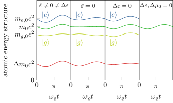
includes the dimensionless coupling constant of the source mass. The dilaton field consists of two contributions: (i) The first part introduces modifications of the gravitational potential leading to EP violations. Di Pumpo et al. (2023) For example, it implies that the gravitational acceleration may be state-dependent, providing hints to extend general relativity. (ii) The second part is an oscillating background field which can model cosmic DM. Hees et al. (2018) It behaves like a plane wave with the amplitude and wave vector at frequency . The initial phase is unknown, so that only a stochastic background of cosmic DM will be observed by the detector. Through its coupling to the energies of the individual states and by that through mass-energy equivalence to the mass of the atom, see Fig. 1, this oscillating background field directly influences both the COM motion and the atomic transition frequency. In turn, such effects induce signatures of DM in the detector’s signal.
Incorporating is not straightforward since one has to perform a non-relativistic limit of a dilaton-modified field theory to avoid operator-ordering issues. However, galactic and cosmic observations Tulin and Yu (2018); Geraci and Derevianko (2016); Arvanitaki et al. (2018) suggest small momenta compared to the rest mass of the dilaton, such that we assume in the following. Thus, the dilaton field’s frequency reduces to its Compton frequency and is solely determined by its mass . In this case, the dimensionless dilaton amplitude Hees et al. (2016); Filzinger et al. (2023) becomes
| (4) |
where the DM energy density is compared to the energy scale given by the Planck mass and a volume defined by the Planck length , with the gravitational constant .
In addition, one could model the coupling of the dilaton field to the source of the gravitational field by yet another dilaton field, possibly incoherent to the one interacting with the atoms. However, we assume that only one field is present, but allow for a phase shift compared to the oscillation of the dilaton field. Hence, we model the time-dependent modulation of the gravitational acceleration via
| (5) |
where is the phase of the dilaton field interacting with the atoms. For example, a phase shift of corresponds to an oscillation of the atoms and gravitational acceleration out of phase. We still can include incoherence between the dilaton-induced atomic properties and a gravitational modification by averaging independently over and in analogy to the treatment discussed below.
III Dark-matter-induced Perturbations on Atoms
With these insights, we expand the Hamiltonian from Eq. (1) with respect to , the unperturbed mass defect , and . As a result, in first order the state-dependent mass can be replaced by
| (6) |
including the unperturbed mean mass and different dimensionless modifications summarized in Table 1 with to denote state-dependent perturbations. We observe the following effects: The mean mass oscillates due to and thereby influencing the COM motion. The dimensionless mass defect gets further modified by , which results in the oscillation of the transition energy explained below.
| Cause | Parameter | Definition |
|---|---|---|
| mean mass | ||
| mass defect | ||
| mass defect | ||
| mean coupling | ||
| differential coupling | ||
| mean-mass osci. | ||
| state-dep. osci. | ||
| osci. of gravity | ||
| mean-mass EP viol. | ||
| state-dep. EP viol. |
Furthermore, the dilaton field effectively leads to a modification of the gravitational acceleration which becomes state dependent, i. e.,
| (7) |
where parametrizes EP violations between different atomic species depending on the mean coupling of the dilaton field to the atom. Schlippert et al. (2014); Di Pumpo et al. (2021); Barrett et al. (2022) An EP violation between different internal states Zhang et al. (2020); Di Pumpo et al. (2023) is encoded in . In addition, the gravitational acceleration changes dynamically via through the DM coupling to the source mass.
We separate the resulting Hamiltonian
| (8) |
into an unperturbed part and perturbations of the rest mass, of the kinetic energy, and of the potential energy. Besides, we generalize to to allow for time-dependent changes of the internal state. We discuss the explicit form of these four contributions in the following:
(i) The unperturbed Hamiltonian
| (9) |
describes a particle of mean mass moving in a linear gravitational potential without any state-dependent effects or internal structure.
(ii) The rest-mass perturbation
| (10) |
does not affect the motion of the atom, but changes the Compton frequency and atomic transition frequency . The phase measured by atomic clocks, Mach-Zehnder and comparable interferometers is not affected by modifications of the Compton frequency to lowest order.111 The Compton frequency is modified to . If both internal states couple identically to the dilaton field, i. e.,, , the change of the Compton frequency is directly proportional to , in contrast to the atomic transition frequency. However, they are sensitive to the atomic transition frequency between both internal states, which is modified to
| (11) |
The unperturbed atomic transition frequency is connected to the mass defect and is modulated by an oscillation with amplitude . Here, is the mean coupling of both internal states to the dilaton, whereas is the difference of their coupling constants, see Table 1. Commonly, it is assumed that is proportional to the atomic transition frequency, Arvanitaki, Huang, and Van Tilburg (2015); Arvanitaki et al. (2018); Badurina, Blas, and McCabe (2022); Hees et al. (2018); Safronova et al. (2018) i. e., the coupling of the dilaton field to both internal states is identical resulting in . Since the details of the coupling are a priori unknown, it is important to allow a different coupling of both internal states, i. e., to allow for . Generally, is a linear combination of both the Compton and the atomic transition frequency with respect to the different coupling parameters. While the coupling parameters and may be of very different orders, the Compton and atomic transition frequency also differ by multiple orders of magnitude so that in principle both contributions to have to be considered. Remarkably, the change of the atomic transition frequency depends on the Compton frequency, which could enhance the DM signature in the detector. Besides, an observable change in the atomic transition frequency present for Raman Zhan et al. (2020) or microwave transitions cannot be completely ruled out. Such transitions are relatively simple to implement and benefit from a much lower recoil velocity, suppressing the impact of gravity-gradient noise.
(iii) The kinetic-energy perturbation
| (12) |
is caused by changes in affects the COM motion. The DM-induced oscillation of the mean mass leads to a time-dependent kinetic energy. Additional state-dependent contributions arise from the mass defect , i. e., the ground state gains kinetic energy while the excited state loses kinetic energy. Further state-dependent mass oscillations arise due to the dilaton field encoded in .
(iv) The potential-energy perturbation
| (13) |
due to changes in both and also affects the COM motion, similar to . However, we notice more contributions: An additional shift of the gravitational acceleration due to the mean-mass EP violation occurs. This shift is relevant for tests of the universality of free fall between different atomic species. Similarly, differential accelerations between the atom in different internal states are encoded in , which is a different facet of possible EP violations, e. g., relevant for tests of the universality of clock rates. Further, we observe a global sign difference in and compared to the unperturbed case. Thus, it raises the expectation that some perturbations contribute twice.
As a side note we mention that both and depend on the perturbation parameters and . In principle, they include products of a dilaton coupling with , which are next order in perturbation. Therefore, they are omitted in further calculations and enclosed in Table 1 by braces.
IV Dark-matter Signal in Atom Gradiometers
Quantum sensors such as atomic clocks or atom interferometers are affected Safronova et al. (2018) by the previously derived perturbations. We focus on the signal observed by DM detectors generated from light-pulse atom interferometers. Such high-precision quantum sensors have been proposed for DM searches, Derevianko and Pospelov (2014); Arvanitaki, Huang, and Van Tilburg (2015); Geraci and Derevianko (2016); Arvanitaki et al. (2018); Badurina et al. (2023) whose signal can be enhanced by multi-diamond Graham et al. (2016); Schubert et al. (2019, 2021); Di Pumpo, Friedrich, and Giese (2023) along with large-momentum-transfer techniques. Chiow et al. (2011); Graham et al. (2013); Gebbe et al. (2021) To focus on the fundamental effects on these detectors, we study an atomic Mach-Zehnder interferometer (MZI) cf. Fig. 2 without transferring large momenta. However, the treatment introduced below can easily be generalized to different interferometer types and geometries.
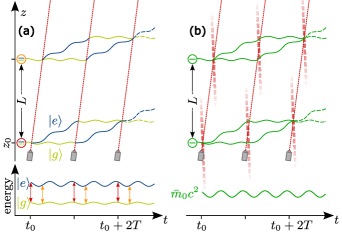
In an MZI, the wave packet is initially split by a beam-splitter pulse into two separate arms. One arm continues along the initial path, while the atoms on the other arm gain momentum due to diffraction, so that the arms become spatially separated. After an interrogation time , a mirror pulse interchanges the momenta of the two arms. At the final time of , a second beam-splitter pulse interferes both arms, resulting in two output ports. Each interaction of the atoms with light that transfers momentum might also change their internal state. Here, the specific implementation is the key for the sensitivity of a detector.
In delta-pulse approximation Schleich, Greenberger, and Rasel (2013); Funai and Martín-Martínez (2019) the effect of light-matter interaction on the atomic motion is described by an effective arm-dependent potential Ufrecht and Giese (2020)
| (14) |
with being the (effective) wave vector acting at time , transferring the momentum on arm , and denoting the Delta distribution. We assume that both arms are diffracted at the same time, neglecting the finite speed of light on the scale of the arm separation. Tan, Shao, and Hu (2017) Moreover, we do not include frequency chirps necessary in terrestrial, vertical configurations and omit the standard laser-phase contribution.
This interaction allows for different momentum-transfer mechanisms and can in principle incorporate large momentum transfer. Typically, the interaction is categorized into single-photon Bott, Di Pumpo, and Giese (2023) and (counter-propagating) two-photon Hartmann et al. (2020) transitions. In the former, simply corresponds to the laser’s wave vector, while in the latter, is the effective wave vector given by the sum of both lasers’ wave vectors. Two-photon transitions suffer from laser-phase noise in differential setups with long baselines, which is suppressed for single-photon transitions. Nevertheless, two-photon transitions are generally more flexible. They allow to only transfer momentum without changing the internal state (Bragg) and drive effectively hyperfine-structure transitions while transferring momentum that corresponds to optical wavelengths (Raman).
Assuming for all interaction times and vanishing gravity gradients leads to a closed, unperturbed MZI. Deviations are introduced by the dilaton field as discussed in Eqs. (10)–(13). In a perturbative treatment, Ufrecht and Giese (2020) we find to first order the phase
| (15) |
with the wave packet’s initial position , as well as initial momentum , depending on the time at which the interferometer is initialized. It includes the standard phase of an MZI, which is perturbed by the contributions and induced by the dilaton field, compare Table 2 in Appendix A for their explicit expressions.
Common-mode operation of two MZIs spatially separated by the distance , e. g., where the first MZI is located at and the second one at , suppresses noise and the dominant phase for vanishing gravity gradients. Graham et al. (2013) We account for the finite speed of light on the separation scale of the two interferometers, but not on the extent of the arm separation of a single one. The first MZI starts its sequence at time with an initial momentum of the wave packet, while the second interferometer starts at time with an initial momentum . Subtracting the phases of both interferometers gives rise to the differential phase, which in our approximation only depends on dilaton-introduced perturbations
| (16) |
with and the propagation delay of the light pulse.
Since the dilaton phase may vary, we can only measure this stochastic background and we therefore have to average. Thus, we assume a uniform distribution of in accordance with the principle of maximum entropy. Jaynes (1957) The signal amplitude Arvanitaki et al. (2018)
| (17) |
is the square of the phase difference averaged over . Due to the square, various correlations of the individual phases contribute.
In the following we identify dominant contributions to the signal, i. e., , for different experimental realizations, namely for single-photon-type and Bragg-type interferometers.
V Single-Photon Interferometers
Many planned DM detectors Abe et al. (2021); Badurina et al. (2020) based on atom interferometry rely on single-photon transitions, due to their intrinsic suppression of laser-phase noise. Yu and Tinto (2011); Graham et al. (2016) In this section, we consider the effects of the dilaton field on such interferometers and focus on the dominant contributions of the observed signal amplitude. Using single-photon transitions for atomic diffraction not only changes the momentum of the atom, but also its internal state. The results discussed in this section therefore also transfer to Raman transitions, also planned for some sensors, Zhan et al. (2020) where only the frequency scales have to be adjusted.
We first focus on the phase difference introduced by the modified atomic transition frequency cf. Eq. (11) which gives rise to
| (18) |
where the timescale is proportional to and is listed in Table 3 in Appendix A. Recalling from Eq. (4) shows that this contribution plays an important role in the search for ultralight DM. In particular, the change of the atomic transition frequency yields the dominant contribution
| (19) |
to the signal amplitude, with . We refer to factors like as interferometric factors that include the interrogation-mode function. Di Pumpo, Friedrich, and Giese (2023) Perturbations and scaling factors like are independent of the explicit interferometer geometry and appear in a similar form for different geometries, including those with large momentum transfer.
Equation (19) is a generalization of other treatments of atom-interferometric DM detectors Arvanitaki et al. (2018) but has a similar form. In fact, the differential coupling is usually neglected, which introduces another frequency scale. In principle, this contribution also arises for Raman-type interferometers, where the atomic energy difference is in the microwave range and much smaller than for optical transitions. However, due to the coupling to the Compton frequency that is orders of magnitude larger, one can also expect a sensitivity to the parameter for Raman setups. The same holds true for single-photon transitions between hyperfine states in the microwave range. For this type of transitions, in contrary, the momentum transfer is negligible, resulting in interferometers that are less sensitive to gravity-gradient noise.
As discussed above, generally the coupling scheme is unknown so that both and might contribute. Since their order of magnitude is unknown, we consider in the following two limiting cases: Either the coupling of both internal states is completely identical, i. e., , or exactly opposite, i. e., .
V.1 Vanishing Mean Coupling ()
For vanishing mean coupling, the change of the atomic transition frequency reduces to . Hence, the relevant scale is given by the Compton frequency and not by the atomic transition frequency. This is different to what is usually postulated in most treatments for AIs and clocks, where is assumed. Since generally applies, we expect a larger suppression of contributions which do not originate from the clock phase but keep in mind that we probe for a different coupling parameter. For example, strontium is a promising candidate Loriani et al. (2019) for future single-photon AIs Hu et al. (2017); Rudolph et al. (2020) and gives rise to .
Consequently, we neglect all for as their scale factors have to be compared to the Compton frequency, and arrive at the signal amplitude
| (20) |
We recognize the twofold effect of the Compton frequency: On the one hand it leads to the suppression of phase contributions competing with . And on the other hand, it enhances the signal. This result also persists for setups where small transition frequencies are used, e. g., hyperfine or Raman transitions. In this case, the Compton frequency clearly sets the relevant scale, even though the coupling parameter might be small.
V.2 Vanishing Differential Coupling ()
If both internal states couple identically to the dilaton field, as assumed in most previous treatments, the modulation amplitude of the atomic transition frequency takes the form . Hence, the relevant scale is now the atomic transition frequency. For single-photon transitions, the atomic transition frequency benefits from an optical regime and has a clear advantage over hyperfine or Raman transitions. Similar to the previous discussion,
| (21) |
is the dominant contribution. But, by decreasing the relevant scale by several orders of magnitude, we include as next-order contributions to the signal amplitude.
After averaging over , the surviving next-order contributions to the signal amplitude , , and (listed in this order) give rise to
| (22) |
with the recoil frequency and the initial mean momentum .
The dominant part of the signal, i. e., , has already been discussed. Arvanitaki et al. (2018) We provide the next sub-leading corrections and observe that even in spaceborne experiments provides a purely kinetic contribution. Additionally, for terrestrial setups long interrogation times increase the significance of . The contribution induced by oscillating gravity vanishes for an in-phase oscillation, i. e., , but can be enhanced by .
V.3 Influence of Both Couplings
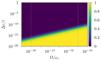
Since one usually neglects the differential coupling , we briefly discuss its influence for different values of . For that, we compare this approximation to the full expression by studying the ratio . It is plotted in Fig. 3 as a function of and . It shows a drastic change between the two regimes discussed above. However, Fig. 3 gives a hint where the general signal-amplitude contribution has to be considered in the analysis for an expected range of coupling parameters and depending on the specific atomic species and transition frequency. The figure highlights that even if the ratio is small, it can be compensated due to the different order of magnitude of the transition frequency and the Compton frequency.
VI Bragg-Type Interferometers ()
Finally, we turn to Bragg-type MZIs, where a two-photon process is used to only transfer momentum without changing the internal state. Therefore, we have , which directly implies that such interferometers are only susceptible to the mean coupling of the atom to the dilaton field. While there have been proposals for DM detectors that focus on the COM motion Geraci and Derevianko (2016) and not on the internal structure of the atom, which effectively corresponds to Bragg-based setups, differential configurations have not yet been discussed in detail. Currently, in the context of very-long-baseline atom interferometry differential setups, which can in principle be used for DM detection, are envisioned to rely on Bragg diffraction, e. g., MAGIS-100, Abe et al. (2021) MIGA, Canuel et al. (2018) or ZAIGA. Zhan et al. (2020)
For Bragg-type interferometers only a few phase contributions remain in the differential setup cf. Table 2 in Appendix A, some of which have been also calculated before. Geraci and Derevianko (2016) These terms also arise for single-photon transitions, where, as previously discussed, the clock contribution dominates. Among these remaining phase contributions, it is not straightforward to determine which one is the dominant one in the signal amplitude. We therefore list all of them in Table 5 in Appendix A. With the help of this overview one can identify three different scales in the signal amplitude, independent of the violation parameters and interferometric factors. For each experiment it has to be checked individually which scale is the dominant one. However, the limiting case , which is important for spaceborne experiments or horizontal setups like the MIGA project, simplifies the signal amplitude to
| (23) |
where the interferometric factor originates from , which is the only remaining contribution cf. Table 5. Since all other terms vanish, these types of setups are less susceptible for ultralight DM searches compared to terrestrial setups, where gravity-induced contributions are present.
In summary, we can identify different relevant scales in the various limiting cases by comparing Eqs. (20)–(23). This comparison leads to . We see that the single-photon-type interferometers benefit from the Compton and atomic transition frequency, whereas Bragg-type interferometers in zero gravity only depend on the recoil frequency.
VII Conclusions
In our article, we demonstrated that assuming a linear scaling of the dark-matter-induced change of the atomic transition frequency with the unperturbed transition frequency is only an approximation for vanishing differential coupling that is made in most discussions. Geraci and Derevianko (2016); Arvanitaki et al. (2018); Badurina et al. (2023) Atom interferometers that rely on the change of internal states, e. g., single-photon or Raman transitions, are susceptible to both types of coupling, where the signal is dominated by clock-type phases. Norcia, Cline, and Thompson (2017) In these cases, the atomic transition and Compton frequency are relevant frequency scales weighted by the mean and differential coupling of both states to dark matter, respectively. However, Bragg-type atom interferometers that preserve the internal state are less susceptible to dark matter in the sense, that they only depend on the mean coupling and the recoil frequency. Therefore, they can only measure effects on the motion like accelerometers. Graham et al. (2016); Geraci and Derevianko (2016)
Our results support the dark-matter search with single-photon atom interferometers in terrestrial setups since their signal profits from any dark-matter-related contributions. Nevertheless, a detailed noise analysis is necessary. Additionally, various mechanisms for atomic diffraction can be used to isolate different coupling parameters, e. g., the results from spaceborne Bragg-type setups can give bounds on the mean coupling. These limits can be combined with the results from other setups to give bounds to both independent coupling parameters and make connections to the tests of the Einstein equivalence principle.
In perspective, a generalization of our treatment to different geometries might be useful to boost dark-matter signatures in the signal, e. g., large-momentum-transfer techniques. In this context the effect of the modified Compton frequency can be studied in recoil measurements for dark-matter detection or Ramsey-Bordé-type interferometers. Bordé (1989) Following current developments in gravitational-wave detection, various differential schemes can be considered and atom-interferometer-based networks Badurina et al. (2020); Figueroa, Budker, and Rasel (2021) can be simultaneously used for dark-matter searches and the detection of gravitational waves. Finally, implications for quantum-clock interferometry Loriani et al. (2019); Zych et al. (2011) can be studied, i. e., propagating a superposition of internal states along each interferometer arm, to focus on the effect of the different degrees of freedom.
Acknowledgements.
We thank F. Di Pumpo, A. Friedrich, A. Geyer, C. Ufrecht, as well as the QUANTUS and INTENTAS teams for fruitful and interesting discussions. The QUANTUS and INTENTAS projects are supported by the German Space Agency at the German Aerospace Center (Deutsche Raumfahrtagentur im Deutschen Zentrum für Luft- und Raumfahrt, DLR) with funds provided by the Federal Ministry for Economic Affairs and Climate Action (Bundesministerium für Wirtschaft und Klimaschutz, BMWK) due to an enactment of the German Bundestag under Grant Nos. 50WM2250E (QUANTUS+), as well as 50WM2177 (INTENTAS). E.G. thanks the German Research Foundation (Deutsche Forschungsgemeinschaft, DFG) for a Mercator Fellowship within CRC 1227 (DQ-mat).Author Declarations
Conflict of Interest
The authors have no conflicts to disclose.
Author Contributions
Daniel Derr Conceptualization (supporting); Formal analysis (lead); Investigation (lead); Validation (equal); Visualization (lead); Writing - original draft (lead); Writing - review and editing (equal).
Enno Giese Conceptualization (lead); Formal analysis (supporting); Funding acquisition (lead); Investigation (supporting); Supervision (lead); Validation (equal); Visualization (supporting); Writing - original draft (supporting); Writing - review and editing (equal).
Data Availability
The data that support the findings of this study are available within the article.
Appendix A Definitions, Phases and Signal Contributions
In this appendix, we summarize the main results and various contributions to the interferometer phase, as well as the signal amplitude. To keep the description as simple as possible, we have collected these expressions in tables that are given here, to keep the main body of our article focused on the main results. Nevertheless, the exact equations are provided here for completeness and can be used for further studies.
The phase contributions induced by dark matter into the interference signal of Mach-Zehnder interferometers are listed in Table 2. Here, we connect the individual phase contributions to the respective perturbative potential and identify the individual cause. For a compact notation of these expressions, we introduce different time scales defined in Table 3.
These phases serve for the calculation of the signal amplitude, where the variance of the phase differences between two interferometers in a gravimeter is averaged over the phase of the dilaton field. Table 4 summarizes all non-vanishing sub-leading contributions to the signal amplitude of single-photon-like Mach-Zehnder interferometers. Besides a numerical factor, we identify the respective scale, violation parameters, as well as an interferometric factor that depends on the geometry used, the initial momenta and the interrogation-mode function Di Pumpo, Friedrich, and Giese (2023). The same analysis is performed in Table 5 for the case of Bragg-type Mach-Zehnder interferometers. Here, all possible contributions to the signal amplitude are given, as no dominant energy and frequency scale can be identified.
| Perturbative Potential | Origin | Expression | Abbreviation | Phase Contribution | |
| mean-mass oscillation | |||||
| mass defect | |||||
| oscillation of transition energy | |||||
| mean-mass oscillation | |||||
| mass defect | |||||
| oscillation of transition energy | |||||
| EP violation | |||||
| state-dependent EP violation | |||||
| oscillation of gravity | |||||
| oscillation of transition energy | |||||
| mass defect | |||||
| oscillation of transition energy | |||||
| Time Scale | Definition |
|---|---|
| Factor | Scale | Violation Parameters | Interferometric Factor | |||||
|---|---|---|---|---|---|---|---|---|
| Factor | Scale | Violation Parameters | Interferometric Factor | |||||
|---|---|---|---|---|---|---|---|---|
References
References
- Bertone and Hooper (2018) G. Bertone and D. Hooper, “History of dark matter,” Rev. Mod. Phys. 90, 045002 (2018).
- Abe et al. (2021) M. Abe, P. Adamson, M. Borcean, D. Bortoletto, K. Bridges, S. P. Carman, S. Chattopadhyay, J. Coleman, N. M. Curfman, K. DeRose, T. Deshpande, S. Dimopoulos, C. J. Foot, J. C. Frisch, B. E. Garber, S. Geer, V. Gibson, J. Glick, P. W. Graham, S. R. Hahn, R. Harnik, L. Hawkins, S. Hindley, J. M. Hogan, Y. Jiang, M. A. Kasevich, R. J. Kellett, M. Kiburg, T. Kovachy, J. D. Lykken, J. March-Russell, J. Mitchell, M. Murphy, M. Nantel, L. E. Nobrega, R. K. Plunkett, S. Rajendran, J. Rudolph, N. Sachdeva, M. Safdari, J. K. Santucci, A. G. Schwartzman, I. Shipsey, H. Swan, L. R. Valerio, A. Vasonis, Y. Wang, and T. Wilkason, “Matter-wave atomic gradiometer interferometric sensor (MAGIS-100),” Quantum Sci. Technol. 6, 044003 (2021).
- Badurina et al. (2020) L. Badurina, E. Bentine, D. Blas, K. Bongs, D. Bortoletto, T. Bowcock, K. Bridges, W. Bowden, O. Buchmueller, C. Burrage, J. Coleman, G. Elertas, J. Ellis, C. Foot, V. Gibson, M. G. Haehnelt, T. Harte, S. Hedges, R. Hobson, M. Holynski, T. Jones, M. Langlois, S. Lellouch, M. Lewicki, R. Maiolino, P. Majewski, S. Malik, J. March-Russell, C. McCabe, D. Newbold, B. Sauer, U. Schneider, I. Shipsey, Y. Singh, M. A. Uchida, T. Valenzuela, M. van der Grinten, V. Vaskonen, J. Vossebeld, D. Weatherill, and I. Wilmut, “AION: an atom interferometer observatory and network,” J. Cosmol. Astropart. Phys. 2020, 011 (2020).
- Zhan et al. (2020) M.-S. Zhan, J. Wang, W.-T. Ni, D.-F. Gao, G. Wang, L.-X. He, R.-B. Li, L. Zhou, X. Chen, J.-Q. Zhong, B. Tang, Z.-W. Yao, L. Zhu, Z.-Y. Xiong, S.-B. Lu, G.-H. Yu, Q.-F. Cheng, M. Liu, Y.-R. Liang, P. Xu, X.-D. He, M. Ke, Z. Tan, and J. Luo, “ZAIGA: Zhaoshan long-baseline atom interferometer gravitation antenna,” Int. J. Mod. Phys. D 29, 1940005 (2020).
- Arduini et al. (2023) G. Arduini, L. Badurina, K. Balazs, C. Baynham, O. Buchmueller, M. Buzio, S. Calatroni, J. P. Corso, J. Ellis, C. Gaignant, M. Guinchard, T. Hakulinen, R. Hobson, A. Infantino, D. Lafarge, R. Langlois, C. Marcel, J. Mitchell, M. Parodi, M. Pentella, D. Valuch, and H. Vincke, “A Long-Baseline Atom Interferometer at CERN: Conceptual Feasibility Study,” arXiv:2304.00614 (2023).
- Abend et al. (2023) S. Abend et al., “Terrestrial Very-Long-Baseline Atom Interferometry: Workshop Summary,” arXiv:2310.08183 (2023).
- Geraci and Derevianko (2016) A. A. Geraci and A. Derevianko, “Sensitivity of Atom Interferometry to Ultralight Scalar Field Dark Matter,” Phys. Rev. Lett. 117, 261301 (2016).
- Figueroa, Budker, and Rasel (2021) N. L. Figueroa, D. Budker, and E. M. Rasel, “Dark matter searches using accelerometer-based networks,” Quantum Sci. Technol. 6, 034004 (2021).
- Arvanitaki et al. (2018) A. Arvanitaki, P. W. Graham, J. M. Hogan, S. Rajendran, and K. Van Tilburg, “Search for light scalar dark matter with atomic gravitational wave detectors,” Phys. Rev. D 97, 075020 (2018).
- Canuel et al. (2018) B. Canuel, A. Bertoldi, L. Amand, E. Pozzo di Borgo, T. Chantrait, C. Danquigny, M. Dovale Álvarez, B. Fang, A. Freise, R. Geiger, J. Gillot, S. Henry, J. Hinderer, D. Holleville, J. Junca, G. Lefèvre, M. Merzougui, N. Mielec, T. Monfret, S. Pelisson, M. Prevedelli, S. Reynaud, I. Riou, Y. Rogister, S. Rosat, E. Cormier, A. Landragin, W. Chaibi, S. Gaffet, and P. Bouyer, “Exploring gravity with the MIGA large scale atom interferometer,” Sci. Rep. 8, 14064 (2018).
- Canuel et al. (2020a) B. Canuel, S. Abend, P. Amaro-Seoane, F. Badaracco, Q. Beaufils, A. Bertoldi, K. Bongs, P. Bouyer, C. Braxmaier, W. Chaibi, N. Christensen, F. Fitzek, G. Flouris, N. Gaaloul, S. Gaffet, C. L. Garrido Alzar, R. Geiger, S. Guellati-Khelifa, K. Hammerer, J. Harms, J. Hinderer, M. Holynski, J. Junca, S. Katsanevas, C. Klempt, C. Kozanitis, M. Krutzik, A. Landragin, I. Làzaro Roche, B. Leykauf, Y.-H. Lien, S. Loriani, S. Merlet, M. Merzougui, M. Nofrarias, P. Papadakos, F. Pereira Dos Santos, A. Peters, D. Plexousakis, M. Prevedelli, E. M. Rasel, Y. Rogister, S. Rosat, A. Roura, D. O. Sabulsky, V. Schkolnik, D. Schlippert, C. Schubert, L. Sidorenkov, J.-N. Siemß, C. F. Sopuerta, F. Sorrentino, C. Struckmann, G. M. Tino, G. Tsagkatakis, A. Viceré, W. von Klitzing, L. Wörner, and X. Zou, “ELGAR—a European Laboratory for Gravitation and Atom-interferometric Research,” Class. Quantum Grav. 37, 225017 (2020a).
- El-Neaj et al. (2020) El-Neaj et al., “AEDGE: Atomic experiment for dark matter and gravity exploration in space,” EPJ Quantum Technol. 7, 6 (2020).
- Savoie et al. (2018) D. Savoie, M. Altorio, B. Fang, L. A. Sidorenkov, R. Geiger, and A. Landragin, “Interleaved atom interferometry for high-sensitivity inertial measurements,” Sci. Adv. 4, eaau7948 (2018).
- Canuel et al. (2020b) B. Canuel, S. Abend, P. Amaro-Seoane, F. Badaracco, Q. Beaufils, A. Bertoldi, K. Bongs, P. Bouyer, C. Braxmaier, W. Chaibi, N. Christensen, F. Fitzek, G. Flouris, N. Gaaloul, S. Gaffet, C. L. G. Alzar, R. Geiger, S. Guellati-Khelifa, K. Hammerer, J. Harms, J. Hinderer, M. Holynski, J. Junca, S. Katsanevas, C. Klempt, C. Kozanitis, M. Krutzik, A. Landragin, I. L. Roche, B. Leykauf, Y. H. Lien, S. Loriani, S. Merlet, M. Merzougui, M. Nofrarias, P. Papadakos, F. P. dos Santos, A. Peters, D. Plexousakis, M. Prevedelli, E. M. Rasel, Y. Rogister, S. Rosat, A. Roura, D. O. Sabulsky, V. Schkolnik, D. Schlippert, C. Schubert, L. Sidorenkov, J. N. Siemß, C. F. Sopuerta, F. Sorrentino, C. Struckmann, G. M. Tino, G. Tsagkatakis, A. Viceré, W. von Klitzing, L. Woerner, and X. Zou, “Technologies for the ELGAR large scale atom interferometer array,” arXiv:2007.04014 (2020b).
- Hartmann et al. (2020) S. Hartmann, J. Jenewein, E. Giese, S. Abend, A. Roura, E. M. Rasel, and W. P. Schleich, “Regimes of atomic diffraction: Raman versus Bragg diffraction in retroreflective geometries,” Phys. Rev. A 101, 053610 (2020).
- Hu et al. (2017) L. Hu, N. Poli, L. Salvi, and G. M. Tino, “Atom interferometry with the Sr optical clock transition,” Phys. Rev. Lett. 119, 263601 (2017).
- Hu et al. (2019) L. Hu, E. Wang, L. Salvi, J. N. Tinsley, G. M. Tino, and N. Poli, “Sr atom interferometry with the optical clock transition as a gravimeter and a gravity gradiometer,” Class. Quantum Gravity 37, 014001 (2019).
- Rudolph et al. (2020) J. Rudolph, T. Wilkason, M. Nantel, H. Swan, C. M. Holland, Y. Jiang, B. E. Garber, S. P. Carman, and J. M. Hogan, “Large momentum transfer clock atom interferometry on the 689 nm intercombination line of strontium,” Phys. Rev. Lett. 124, 083604 (2020).
- Bott, Di Pumpo, and Giese (2023) A. Bott, F. Di Pumpo, and E. Giese, “Atomic diffraction from single-photon transitions in gravity and Standard-Model extensions,” AVS Quantum Sci. 5, 044402 (2023).
- Ludlow et al. (2015) A. D. Ludlow, M. M. Boyd, J. Ye, E. Peik, and P. O. Schmidt, “Optical atomic clocks,” Rev. Mod. Phys. 87, 637–701 (2015).
- Yu and Tinto (2011) N. Yu and M. Tinto, “Gravitational wave detection with single-laser atom interferometers,” Gen. Relativ. Gravit. 43, 1943–1952 (2011).
- Graham et al. (2013) P. W. Graham, J. M. Hogan, M. A. Kasevich, and S. Rajendran, “New method for gravitational wave detection with atomic sensors,” Phys. Rev. Lett. 110, 171102 (2013).
- Derevianko and Pospelov (2014) A. Derevianko and M. Pospelov, “Hunting for topological dark matter with atomic clocks,” Nat. Phys. 10, 933–936 (2014).
- Arvanitaki, Huang, and Van Tilburg (2015) A. Arvanitaki, J. Huang, and K. Van Tilburg, “Searching for dilaton dark matter with atomic clocks,” Phys. Rev. D 91, 015015 (2015).
- Norcia, Cline, and Thompson (2017) M. A. Norcia, J. R. K. Cline, and J. K. Thompson, “Role of atoms in atomic gravitational-wave detectors,” Phys. Rev. A 96, 042118 (2017).
- Graham et al. (2016) P. W. Graham, D. E. Kaplan, J. Mardon, S. Rajendran, and W. A. Terrano, “Dark matter direct detection with accelerometers,” Phys. Rev. D 93, 075029 (2016).
- Badurina, Blas, and McCabe (2022) L. Badurina, D. Blas, and C. McCabe, “Refined ultralight scalar dark matter searches with compact atom gradiometers,” Phys. Rev. D 105, 023006 (2022).
- Damour and Polyakov (1994) T. Damour and A. M. Polyakov, “The string dilation and a least coupling principle,” Nucl. Phys. B 423, 532–558 (1994).
- Alves and Bezerra (2000) M. Alves and V. Bezerra, “Dilaton gravity with a nonminimally coupled scalar field,” Int. J. Mod. Phys. D 09, 697–703 (2000).
- Buckley, Feld, and Gonçalves (2015) M. R. Buckley, D. Feld, and D. Gonçalves, “Scalar simplified models for dark matter,” Phys. Rev. D 91, 015017 (2015).
- Kimball and van Bibber (2023) D. F. J. Kimball and K. van Bibber, The Search for Ultralight Bosonic Dark Matter (Springer Nature, 2023).
- Badurina et al. (2023) L. Badurina, V. Gibson, C. McCabe, and J. Mitchell, “Ultralight dark matter searches at the sub-Hz frontier with atom multigradiometry,” Phys. Rev. D 107, 055002 (2023).
- Antypas et al. (2022) D. Antypas et al., “New Horizons: Scalar and Vector Ultralight Dark Matter,” arXiv:2203.14915 (2022).
- Filzinger et al. (2023) M. Filzinger, S. Dörscher, R. Lange, J. Klose, M. Steinel, E. Benkler, E. Peik, C. Lisdat, and N. Huntemann, “Improved Limits on the Coupling of Ultralight Bosonic Dark Matter to Photons from Optical Atomic Clock Comparisons,” Phys. Rev. Lett. 130, 253001 (2023).
- Safronova et al. (2018) M. S. Safronova, D. Budker, D. DeMille, D. F. J. Kimball, A. Derevianko, and C. W. Clark, “Search for new physics with atoms and molecules,” Rev. Mod. Phys. 90, 025008 (2018).
- Giulini (2012) D. Giulini, “Equivalence Principle, Quantum Mechanics, and Atom-Interferometric Tests,” in Quantum Field Theory and Gravity: Conceptual and Mathematical Advances in the Search for a Unified Framework, edited by F. Finster, O. Müller, M. Nardmann, J. Tolksdorf, and E. Zeidler (Birkhäuser, Basel, 2012) pp. 345–370.
- Will (2014) C. M. Will, “The confrontation between general relativity and experiment,” Living Rev. Relativ. 17, 4 (2014).
- Schlippert et al. (2014) D. Schlippert, J. Hartwig, H. Albers, L. L. Richardson, C. Schubert, A. Roura, W. P. Schleich, W. Ertmer, and E. M. Rasel, “Quantum test of the universality of free fall,” Phys. Rev. Lett. 112, 203002 (2014).
- Barrett et al. (2022) B. Barrett, G. Condon, L. Chichet, L. Antoni-Micollier, R. Arguel, M. Rabault, C. Pelluet, V. Jarlaud, A. Landragin, P. Bouyer, and B. Battelier, “Testing the universality of free fall using correlated – atom interferometers,” AVS Quantum Sci. 4, 014401 (2022).
- Asenbaum et al. (2020) P. Asenbaum, C. Overstreet, M. Kim, J. Curti, and M. A. Kasevich, “Atom-interferometric test of the equivalence principle at the level,” Phys. Rev. Lett. 125, 191101 (2020).
- Di Pumpo et al. (2021) F. Di Pumpo, C. Ufrecht, A. Friedrich, E. Giese, W. P. Schleich, and W. G. Unruh, “Gravitational redshift tests with atomic clocks and atom interferometers,” PRX Quantum 2, 040333 (2021).
- Di Pumpo et al. (2023) F. Di Pumpo, A. Friedrich, C. Ufrecht, and E. Giese, “Universality-of-clock-rates test using atom interferometry with scaling,” Phys. Rev. D 107, 064007 (2023).
- Damour and Donoghue (2010) T. Damour and J. F. Donoghue, “Equivalence principle violations and couplings of a light dilaton,” Phys. Rev. D 82, 084033 (2010).
- Damour (2012) T. Damour, “Theoretical aspects of the equivalence principle,” Class. Quantum Gravity 29, 184001 (2012).
- Yudin and Taichenachev (2018) V. Yudin and A. Taichenachev, “Mass defect effects in atomic clocks,” Laser Phys. Lett. 15, 035703 (2018).
- Sonnleitner and Barnett (2018) M. Sonnleitner and S. M. Barnett, “Mass-energy and anomalous friction in quantum optics,” Phys. Rev. A 98, 042106 (2018).
- Schwartz and Giulini (2019) P. K. Schwartz and D. Giulini, “Post-Newtonian Hamiltonian description of an atom in a weak gravitational field,” Phys. Rev. A 100, 052116 (2019).
- Martínez-Lahuerta et al. (2022) V. J. Martínez-Lahuerta, S. Eilers, T. E. Mehlstäubler, P. O. Schmidt, and K. Hammerer, “Ab initio quantum theory of mass defect and time dilation in trapped-ion optical clocks,” Phys. Rev. A 106, 032803 (2022).
- Aßmann, Giese, and Di Pumpo (2023) T. Aßmann, E. Giese, and F. Di Pumpo, “Quantum field theory for multipolar composite bosons with mass defect and relativistic corrections,” arXiv:2307.06110 (2023).
- Di Pumpo et al. (2022) F. Di Pumpo, A. Friedrich, A. Geyer, C. Ufrecht, and E. Giese, “Light propagation and atom interferometry in gravity and dilaton fields,” Phys. Rev. D 105, 084065 (2022).
- Hees et al. (2016) A. Hees, J. Guéna, M. Abgrall, S. Bize, and P. Wolf, “Searching for an Oscillating Massive Scalar Field as a Dark Matter Candidate Using Atomic Hyperfine Frequency Comparisons,” Phys. Rev. Lett. 117, 061301 (2016).
- Hees et al. (2018) A. Hees, O. Minazzoli, E. Savalle, Y. V. Stadnik, and P. Wolf, “Violation of the equivalence principle from light scalar dark matter,” Phys. Rev. D 98, 064051 (2018).
- Tulin and Yu (2018) S. Tulin and H.-B. Yu, “Dark matter self-interactions and small scale structure,” Phys. Rep. 730, 1–57 (2018).
- Zhang et al. (2020) K. Zhang, M.-K. Zhou, Y. Cheng, L.-L. Chen, Q. Luo, W.-J. Xu, L.-S. Cao, X.-C. Duan, and Z.-K. Hu, “Testing the Universality of Free Fall by Comparing the Atoms in Different Hyperfine States with Bragg Diffraction,” Chin. Phys. Lett. 37, 043701 (2020).
- Note (1) The Compton frequency is modified to . If both internal states couple identically to the dilaton field, i. e.,, , the change of the Compton frequency is directly proportional to , in contrast to the atomic transition frequency.
- Schubert et al. (2019) C. Schubert, D. Schlippert, S. Abend, E. Giese, A. Roura, W. P. Schleich, W. Ertmer, and E. M. Rasel, “Scalable, symmetric atom interferometer for infrasound gravitational wave detection,” arXiv:1909.01951 (2019).
- Schubert et al. (2021) C. Schubert, S. Abend, M. Gersemann, M. Gebbe, D. Schlippert, P. Berg, and E. M. Rasel, “Multi-loop atomic Sagnac interferometry,” Sci. Rep. 11, 16121 (2021).
- Di Pumpo, Friedrich, and Giese (2023) F. Di Pumpo, A. Friedrich, and E. Giese, “Optimal baseline exploitation in vertical dark-matter detectors based on atom interferometry,” arXiv:2309.04207 (2023).
- Chiow et al. (2011) S. Chiow, T. Kovachy, H. Chien, and M. A. Kasevich, “ Large Area Atom Interferometers,” Phys. Rev. Lett. 107, 130403 (2011).
- Gebbe et al. (2021) M. Gebbe, J.-N. Siemß, M. Gersemann, H. Müntinga, S. Herrmann, C. Lämmerzahl, H. Ahlers, N. Gaaloul, C. Schubert, K. Hammerer, S. Abend, and E. M. Rasel, “Twin-lattice atom interferometry,” Nat. Commun. 12, 1–7 (2021).
- Schleich, Greenberger, and Rasel (2013) W. P. Schleich, D. M. Greenberger, and E. M. Rasel, “A representation-free description of the Kasevich–Chu interferometer: a resolution of the redshift controversy,” New J. Phys. 15, 013007 (2013).
- Funai and Martín-Martínez (2019) N. Funai and E. Martín-Martínez, “Faster-than-light signaling in the rotating-wave approximation,” Phys. Rev. D 100, 065021 (2019).
- Ufrecht and Giese (2020) C. Ufrecht and E. Giese, “Perturbative operator approach to high-precision light-pulse atom interferometry,” Phys. Rev. A 101, 053615 (2020).
- Tan, Shao, and Hu (2017) Y.-J. Tan, C.-G. Shao, and Z.-K. Hu, “Time delay and the effect of the finite speed of light in atom gravimeters,” Phys. Rev. A 96, 023604 (2017).
- Jaynes (1957) E. T. Jaynes, “Information Theory and Statistical Mechanics,” Phys. Rev. 106, 620–630 (1957).
- Loriani et al. (2019) S. Loriani, D. Schlippert, C. Schubert, S. Abend, H. Ahlers, W. Ertmer, J. Rudolph, J. M. Hogan, M. A. Kasevich, E. M. Rasel, and N. Gaaloul, “Atomic source selection in space-borne gravitational wave detection,” New J. Phys. 21, 063030 (2019).
- Bordé (1989) C. J. Bordé, “Atomic interferometry with internal state labelling,” Phys. Lett. A 140, 10–12 (1989).
- Zych et al. (2011) M. Zych, F. Costa, I. Pikovski, and Č. Brukner, “Quantum interferometric visibility as a witness of general relativistic proper time,” Nat. Commun. 2, 505 (2011).