KiDS-1000 cosmology: Combined second- and third-order shear statistics

Context. This paper performs the first cosmological parameter analysis of the KiDS-1000 data with second- and third-order shear statistics. This work builds on a series of papers that describe the roadmap to third-order shear statistics.
Methods. We derive and test a combined model of the second-order shear statistic, namely the COSEBIs and the third-order aperture mass statistics ${\expectationvalue{\mathcal{M}_{\mathrm{ap}}^{3}}}$ in a tomographic set-up. We validate our pipeline with $N$-body simulations that mock the fourth Kilo Degree survey data release. To model the second- and third-order statistics, we use the latest version of HMcode2020 for the power spectrum and BiHalofit for the bispectrum. Furthermore, we use an analytic description to model intrinsic alignments and hydro-dynamical simulations to model the effect of baryonic feedback processes. Lastly, we decreased the dimension of the data vector significantly by considering for the ${\expectationvalue{\mathcal{M}_{\mathrm{ap}}^{3}}}$ part of the data vector only equal smoothing radii, making a data analysis of the fourth Kilo Degree survey data release using a combined analysis of COSEBIs third-order shear statistic possible.
Results. We first validate the accuracy of our modelling by analysing a noise-free mock data vector assuming the KiDS-1000 error budget, finding a shift in the maximum-a-posterior of the matter density parameter $\Delta\Omega_{\mathrm{m}}<0.02\,\sigma_{\Omega_{\mathrm{m}}}$ and of the structure growth parameter $\Delta S_{8}<0.05\,\sigma_{S_{8}}$. Lastly, we performed the first KiDS-1000 cosmological analysis using a combined analysis of second- and third-order shear statistics, where we constrained $\Omega_{\mathrm{m}}=0.248^{+0.062}_{-0.055}$ and $S_{8}=\sigma_{8}\sqrt{\Omega_{\mathrm{m}}/0.3}=0.772\pm 0.022$. The geometric average on the errors of $\Omega_{\mathrm{m}}$ and $S_{8}$ of the combined statistics increased compared to the second-order statistic by 2.2.

1 Introduction

Gravitational lensing describes the deflection of light by massive objects. Notably, it is sensitive to baryonic and dark matter and is, therefore, ideal for probing the total matter distribution in the Universe. Since the distribution of matter is highly sensitive to cosmological parameters, it is excellent to test and probe the standard model of cosmology, called the $\Lambda$ Cold Dark Matter model ($\Lambda$CDM). Although the $\Lambda$CDM model can describe observations of the early Universe, like the cosmic microwave background (CMB; e.g. Planck Collaboration et al. 2020), or the local Universe, like the observed large-scale structure (LSS) of matter and galaxies (Sánchez et al. 2017), with remarkable accuracy, it is being put under stress due to tension observed between early and local probes. A $\sim 2\,\sigma$ tension is in the structure growth parameter $S_{8}=\sigma_{8}\sqrt{\Omega_{\mathrm{m}}/0.3}$, where $\sigma_{8}$ is the normalisation of the power spectrum and $\Omega_{\mathrm{m}}$ is the total matter density parameter (Hildebrandt et al. 2017; Planck Collaboration et al. 2020; Joudaki et al. 2020; Heymans et al. 2021; Abbott et al. 2022; Di Valentino et al. 2021; Dalal et al. 2023), suggests that the local Universe is less clustered than what is expected from early-time measurements when extrapolated under the LCDM model. If these tensions are not due to systematics, extensions to the $\Lambda$CDM are necessary, which will be tested with the next generation of cosmic shear surveys like Euclid (Laureijs et al. 2011) or the Vera Rubin Observatory Legacy Survey of Space and Time (LSST, Ivezic et al. 2008).

Commonly two-point statistics of weak lensing and galaxy positions are used to infer cosmological parameters since they can be modelled accurately, and systematic inaccuracies are well understood (Schneider et al. 1998; Troxel et al. 2018; Hildebrandt et al. 2017; Hikage et al. 2019; Asgari et al. 2019, 2020; Hildebrandt et al. 2020). Two-point statistics are excellent for capturing the entire information content of a Gaussian random field. However, non-linear gravitational instabilities create a significant amount of non-Gaussian features during the evolution of the Universe, such that the local matter distribution departs strongly from a Gaussian field. Therefore, higher-order statistics are needed to extract all the available information in the local LSS of matter and galaxies. Furthermore, higher-order statistics usually depend differently on cosmological parameters and systematic effects like intrinsic alignment (IA), meaning that a joint investigation of second- and higher-order statistics tightens cosmological parameter constraints (see, e.g. Kilbinger & Schneider 2005; Bergé et al. 2010; Pires et al. 2012; Fu et al. 2014; Pyne & Joachimi 2021). Recently used examples of higher-order statistics are the peak count statistics (Martinet et al. 2018; Harnois-Déraps et al. 2021), persistent homology (Heydenreich et al. 2021), density split statistics (Gruen et al. 2018; Burger et al. 2023), the integrated three-point correlation function used in (Halder et al. 2021; Halder & Barreira 2022), and a second- and third-order convergence moment analysis (Gatti et al. 2022).

This work considers second- and third-order shear statistics, where the former probes the variance and the latter the skewness of the LSS at various scales. Our chosen second-order statistic constitutes the $E_{n}$-modes of the COSEBIs (Schneider et al. 2010), and the third-order statistic ${\expectationvalue{\mathcal{M}_{\mathrm{ap}}^{3}}}$ is described in Schneider et al. (2005) and recently measured in the Dark Energy Survey Year 3 Results (Secco et al. 2022). Furthermore, this work belongs to a series of papers that aim for cosmological parameter analyses using third-order shear statistics. In the first paper Heydenreich et al. (2023, hereafter H23), we validated the analytical fitting formulae for a non-tomographic analysis and the conversion from three-point correlation function (3PCF) of cosmic shear to ${\expectationvalue{\mathcal{M}_{\mathrm{ap}}^{3}}}$. We found that ${\expectationvalue{\mathcal{M}_{\mathrm{ap}}^{3}}}$, although combined from the shear 3PCF at different scales, contain a similar amount of information on $\Omega_{\mathrm{m}}$ and $S_{8}$ as the 3PCF itself. The fact that ${\expectationvalue{\mathcal{M}_{\mathrm{ap}}^{3}}}$ can be measured from 3PCF is very convenient since this allows unbiased estimates for any survey geometry. A fast computation method of the aperture mass statistics by measuring the shear 3PCF is tackled in Porth et al. (2023). Lastly, adding third-order statistics increases the dimension of the data vector significantly, and an analytical expression for the covariance is preferred, which is derived and validated for ${\expectationvalue{\mathcal{M}_{\mathrm{ap}}^{3}}}$ in a non-tomographic setup in Linke et al. (2023). However, as this analysis considers combining second-order statistics with ${\expectationvalue{\mathcal{M}_{\mathrm{ap}}^{3}}}$ in a tomographic setup, and a joint covariance matrix has not been derived yet (Wielders et al. in prep), we still rely on numerical simulations to determine the covariance matrix.

This article presents the first cosmological parameter analysis using the fourth data release of KiDS (KiDS-1000), combining second- and third-order shear statistics. Before we show the cosmological results, we validate several extensions of the analytical model to allow for a tomographic analysis and to include astrophysical effects like IA (e.g. Joachimi et al. 2015) or baryonic feedback processes (Chisari et al. 2015). We aim to find the smallest set of scales that retain most of the cosmological information.

The paper is structured as follows: In Sect. 2, we review the basics of the second- and third-order shear statistics, extend the modelling to a tomographic analysis and describe our method to model the IA analytically. In Sect. 4 we describe the KiDS-1000 data, and in Sect. 5, we introduce the simulation data used to validate our model and to correct it for baryonic feedback processes. In Sect. 6, we briefly review our method to perform cosmological parameter interference. In Sect. 7, and 8, we then validate our analysis pipeline against several systematics. The final cosmological results are presented in Sect. 9, and we conclude in Sect. 10.

2 Theoretical background

This section reviews the basics of weak gravitational lensing formalism and aperture statistics. For more detailed reviews see Bartelmann & Schneider (2001), Hoekstra & Jain (2008), Munshi et al. (2008), Bartelmann (2010), and Kilbinger (2015). In this work, we assume a spatially flat universe, such that the comoving angular-diameter distance $f_{K}[\chi(z)]=\chi(z)$, where $\chi(z)$ is the comoving distance at redshift $z$. Given the matter density $\rho(\boldsymbol{x},z)$ at comoving position $\boldsymbol{x}$ and redshift $z$, the density contrast is $\delta(\boldsymbol{x},z)=\frac{\rho(\boldsymbol{x},z)}{\bar{\rho}(z)}-1$, where $\bar{\rho}(z)$ is the average matter density at redshift $z$. The dimensionless surface mass density or convergence $\kappa$ for sources at redshift $z$ is determined by the line-of-sight integration

$$\kappa(\boldsymbol{\vartheta},z)=\frac{3\Omega_{\mathrm{m}}H_{0}^{2}}{2c^{2}}\int_{0}^{\chi(z)}\differential\chi^{\prime}{} {}\,\frac{\chi^{\prime}\,[\chi(z)-\chi^{\prime}]}{\chi(z)}\frac{\delta(\chi^{\prime}\boldsymbol{\vartheta},z)}{a(\chi^{\prime})}\;,$$ (1)

where $\boldsymbol{\vartheta}$ is the angular postion on the sky, $H_{0}$ is the Hubble constant, and $a$ the scale factor. The second argument of $\delta$ simultaneously describes the radial direction and the cosmological epoch, related through the light-cone condition $|c\differential t|=a(z)\,\differential\chi$.

2.1 Limber projections of power- and bispectrum

Given the Fourier transform $\hat{\delta}$ of the matter density contrast, the matter power spectrum $P_{\delta\delta}(k,z)$ and bispectrum $B_{\delta\delta\delta}(k_{1},k_{2},k_{3},z)$ are

$$\expectationvalue{\hat{\delta}(\boldsymbol{k}_{1},z)\hat{\delta}(\boldsymbol{k}_{2},z)}={} {}(2\pi)^{3}\,\delta_{\mathrm{D}}(\boldsymbol{k}_{1}+\boldsymbol{k}_{2})\,P_{\delta\delta}(k_{1},z)\;,$$ (2)

$$\expectationvalue{\hat{\delta}(\boldsymbol{k}_{1},z)\hat{\delta}(\boldsymbol{k}_{2},z)\hat{\delta}(\boldsymbol{k}_{3},z)}={} {}(2\pi)^{3}\,\delta_{\mathrm{D}}(\boldsymbol{k}_{1}+\boldsymbol{k}_{2}+\boldsymbol{k}_{3})$$

$${}\qquad\times B_{\delta\delta\delta}(k_{1},k_{2},k_{3},z)\;,$$ (3)

where $\delta_{\rm D}$ is the Dirac-delta distribution. The statistical isotropy of the Universe implies that the power- and bispectrum only depend on the moduli of the $k$-vectors.

The projected power- and bispectrum can then be computed using the Limber approximation (Limber 1954; Kaiser & Jaffe 1997; Bernardeau et al. 1997; Schneider et al. 1998; LoVerde & Afshordi 2008),

$$P_{\kappa\kappa}^{(ij)}(\ell)=\int_{0}^{\chi_{\mathrm{max}}}\differential\chi\;\frac{g^{(i)}(\chi)\,g^{(j)}(\chi)}{a^{2}(\chi)}\,P_{\delta\delta}\left[\frac{\ell+1/2}{\chi},z(\chi)\right]\;,\\$$ (4)

$$B_{\kappa\kappa\kappa}^{(ijk)}(\ell_{1},\ell_{2},\ell_{3})={} {}\int_{0}^{\chi_{\mathrm{max}}}\differential\chi\;\frac{g^{(i)}(\chi)\,g^{(j)}(\chi)\,g^{(k)}(\chi)}{a^{3}(\chi)\,\chi}$$

$${}\times B_{\delta\delta\delta}\left[\frac{\ell_{1}}{\chi},\frac{\ell_{2}}{\chi},\frac{\ell_{3}}{\chi},z(\chi)\right]\,,$$ (5)

where $\ell_{3}=|\boldsymbol{\ell}_{1}+\boldsymbol{\ell}_{2}|$, and $g^{(i)}(\chi)$ denotes the lensing efficiency and is defined as

$$g^{(i)}(\chi)=\frac{3\Omega_{\mathrm{m}}H_{0}^{2}}{2c^{2}}\int_{\chi}^{\chi_{\mathrm{max}}}\differential\chi^{\prime}\;n^{(i)}(\chi^{\prime})\,\frac{\chi^{\prime}-\chi}{\chi^{\prime}}\,,$$ (6)

with $n^{(i)}(\chi)$ being the redshift probability distribution of the $i$-th tomographic $z$-bin. Since the Limber approximation breaks down for small values of $\ell$ (Kilbinger et al. 2017), we consider only scales below $4^{\circ}$ for the modelling of ${\expectationvalue{\mathcal{M}_{\mathrm{ap}}^{3}}}$. In principle, we could have also used the modified Limber approximation and shift $\ell_{1,2,3}\rightarrow\ell_{1,2,3}+1/2$, but since we found a difference at maximum for the largest filter radii of $1.5\%$, we have neglected it here. To model the non-linear matter power spectrum $P_{\delta\delta}$, we use the revised HMcode2020 model of Mead et al. (2021) and for the matter bispectrum $B_{\delta\delta\delta}$ the BiHalofit of Takahashi et al. (2020).

2.2 Non-linear alignment model

The impact of galaxy IA is a known contaminating signal to the cosmic shear measurements that needs to be accounted for in all weak lensing studies. In order to model the effects of intrinsic alignment, we use the non-linear alignment (NLA) model (Bridle & King 2007), which is a one-parameter model described as

$$f_{\mathrm{IA}}=-\frac{A_{\mathrm{IA}}\bar{C_{1}}\bar{\rho}(z)}{D_{+}(z)}\,,$$ (7)

where $D_{+}$ is the linear growth factor at redshift $z$, $\bar{C_{1}}=5\times 10^{-14}M_{\odot}^{-1}h^{-2}$ Mpc³, as calibrated in Brown et al. (2002), and $A_{\mathrm{IA}}$ captures the coupling strength between the matter density and the tidal field.

By considering the tidal alignment field $\delta_{\mathrm{I}}$ as a biased tracer of the matter density contrast field $\delta$, neglecting all higher-order bias terms we get

$$\delta_{\mathrm{I}}(\boldsymbol{x},z)=f_{\mathrm{IA}}\delta(\boldsymbol{x},z)\,.$$ (8)

With this, we find that

$$P_{\delta\delta_{\mathrm{I}}}(k,z)=f_{\mathrm{IA}}\,P_{\delta\delta}(k,z)\;,$$ (9)

$$P_{\delta_{\mathrm{I}}\delta_{\mathrm{I}}}(k,z)=f_{\mathrm{IA}}^{2}\,P_{\delta\delta}(k,z)\;,$$ (10)

where $P_{\delta\delta}(k,z)$ is the non-linear matter power spectrum. The projected power spectra then follow to

$$P^{(ij)}_{\mathrm{GI}}(\ell) =\int_{0}^{\infty}\differential\chi\frac{g^{(i)}(\chi)\,n^{(j)}(\chi)}{a(\chi)\chi}\,P_{\delta\delta_{\mathrm{I}}}(\ell/\chi,\chi)\;,$$ (11)

$$P^{(ij)}_{\mathrm{II}}(\ell) =\int_{0}^{\infty}\differential\chi\frac{n^{(i)}(\chi^{\prime})\,n^{(j)}(\chi)}{\chi^{2}}\,P_{\delta_{\mathrm{I}}\delta_{\mathrm{I}}}(\ell/\chi,\chi)\;,$$ (12)

and the total projected power spectrum becomes

$$P^{(ij)}(\ell)=P^{(ij)}_{\mathrm{GG}}(\ell)+P^{(ij)}_{\mathrm{GI}}(\ell)+P^{(ji)}_{\mathrm{GI}}(\ell)+P^{(ij)}_{\mathrm{II}}(\ell)\,.$$ (13)

The term $P^{(ij)}_{\mathrm{GG}}(\ell)=P^{(ij)}_{\kappa\kappa}(\ell)$ describes the actual lensing signal, which is given in Eq. (4) with the weighting kernel in Eq. (6). The II contribution describes how two galaxies spatially close together tend to be aligned. The terms GI and IG describe the fact that high matter density regions align the lower redshift galaxies but also affect the shear of the background galaxies. While the II term is dominant if galaxies of the same tomographic bin are considered, GI and IG start to dominate if galaxies of separated tomographic bins are considered. With $z_{i}<z_{j}$, the term GI is expected to vanish if two separated tomographic bins that have no significant in redshift.

Following the ansatz for modelling IA in the power spectrum, we get

$$B_{\delta\delta\delta_{\mathrm{I}}}(k_{1},k_{2},k_{3},z) =f_{\mathrm{IA}}\,B_{\delta\delta\delta}(k_{1},k_{2},k_{3},z)\,,$$ (14)

$$B_{\delta\delta_{\mathrm{I}}\delta_{\mathrm{I}}}(k_{1},k_{2},k_{3},z) =f_{\mathrm{IA}}^{2}\,B_{\delta\delta\delta}(k_{1},k_{2},k_{3},z)\,,$$ (15)

$$B_{\delta_{\mathrm{I}}\delta_{\mathrm{I}}\delta_{\mathrm{I}}}(k_{1},k_{2},k_{3},z) =f_{\mathrm{IA}}^{3}\,B_{\delta\delta\delta}(k_{1},k_{2},k_{3},z)\,,$$ (16)

where $B_{\delta\delta\delta}$ is the non-linear matter bispectrum, which we calculated with BiHalofit. The projected bispectra are

$$B^{(ijk)}_{\mathrm{GGI}}(\ell_{1},\ell_{2},\ell_{3})=$$

$$\int_{0}^{\infty}\differential\chi\frac{g^{(i)}(\chi)\,g^{(j)}(\chi)\,n^{(k)}(\chi)}{a^{2}(\chi)\chi^{2}}\,B_{\delta\delta\delta_{\mathrm{I}}}(\ell_{1}/\chi,\ell_{2}/\chi,\ell_{3}/\chi,\chi)\,,$$ (17)

$$B^{(ijk)}_{\mathrm{GII}}(\ell_{1},\ell_{2},\ell_{3})=$$

$$\int_{0}^{\infty}\differential\chi\frac{g^{(i)}(\chi)\,n^{(j)}(\chi)\,n^{(k)}(\chi)}{a(\chi)\chi^{3}}\,B_{\delta\delta_{\mathrm{I}}\delta_{\mathrm{I}}}(\ell_{1}/\chi,\ell_{2}/\chi,\ell_{3}/\chi,\chi)\,,$$ (18)

$$B^{(ijk)}_{\mathrm{III}}(\ell_{1},\ell_{2},\ell_{3})=$$

$$\int_{0}^{\infty}\differential\chi\frac{n^{(i)}(\chi)\,n^{(j)}(\chi)\,n^{(k)}(\chi)}{\chi^{4}}\,B_{\delta_{\mathrm{I}}\delta_{\mathrm{I}}\delta_{\mathrm{I}}}(\ell_{1}/\chi,\ell_{2}/\chi,\ell_{3}/\chi,\chi)\,.$$ (19)

The total projected bispectrum is

$$B^{(ijk)}(\hat{\ell}) =B^{(ijk)}_{\mathrm{GGG}}(\hat{\ell})+B^{(ijk)}_{\mathrm{GGI}}(\hat{\ell})+B^{(kij)}_{\mathrm{GGI}}(\hat{\ell})+B^{(jki)}_{\mathrm{GGI}}(\hat{\ell})$$

$$+B^{(ijk)}_{\mathrm{GII}}(\hat{\ell})+B^{(kij)}_{\mathrm{GII}}(\hat{\ell})+B^{(jki)}_{\mathrm{GII}}(\hat{\ell})+B^{(ijk)}_{\mathrm{III}}(\hat{\ell})\,,$$ (20)

where the tuple $\hat{\ell}=(\ell_{1},\ell_{2},\ell_{3})$. The interpretation of all these terms is analogous to the ones from the power spectrum, where $B^{(ijk)}_{GGG}(\hat{\ell})=B^{(ijk)}_{\kappa\kappa\kappa}(\hat{\ell})$ is the actual pure lensing signal given by Eq. (5) with the weighting kernel in Eq. (6).

2.3 Aperture mass statistics

One of the major problems of weak lensing mass reconstruction techniques is the mass-sheet degeneracy (Falco et al. 1985; Schneider & Seitz 1995, hereafter MSD), which corresponds to adding a uniform surface mass density without affecting lensing observables like the shear. However, it is possible to define quantities invariant under the MSD, one example being the aperture mass statistics (Schneider 1996; Bartelmann & Schneider 2001). Another advantage of aperture mass statistics is that they separate the signal into so-called E- and B-modes (Schneider et al. 2002), where, to leading order, the weak gravitational lensing effect can not create B-modes. Lastly, as shown in H23, aperture statistics are an excellent strategy to compress thousands of bins of 3PCF into a few hundred ${\expectationvalue{\mathcal{M}_{\mathrm{ap}}^{3}}}$ bins.

The aperture mass $\mathcal{M}_{\mathrm{ap}}$ at position $\boldsymbol{\vartheta}$ with filter radius $\theta_{\mathrm{ap}}$ is defined through the convergence $\kappa$

$$\mathcal{M}_{\mathrm{ap}}(\boldsymbol{\vartheta};\theta_{\mathrm{ap}})=\int\differential^{2}\vartheta^{\prime}\;U_{\theta_{\mathrm{ap}}}(|\boldsymbol{\vartheta^{\prime}}|)\,\kappa(\boldsymbol{\vartheta}+\boldsymbol{\vartheta^{\prime}})\;,$$ (21)

where $U_{\theta_{\mathrm{ap}}}(\vartheta^{\prime})$ is a compensated filter such that ${\int\differential\vartheta^{\prime}\,\vartheta^{\prime}\,U_{\theta_{\mathrm{ap}}}(\vartheta^{\prime})=0}$. The tangential shear component $\gamma_{\mathrm{t}}$ of the complex shear in Cartesian coordinates $\gamma=\gamma_{1}+\mathrm{i}\gamma_{2}$, is defined as $\gamma_{\mathrm{t}}=-\mathfrak{Re}(\gamma\mathrm{e}^{-2\mathrm{i}\phi})$, where $\phi$ is the polar angle of $\boldsymbol{\vartheta^{\prime}}$. Given the tangential shear $\gamma_{\mathrm{t}}$, the aperture mass $\mathcal{M}_{\mathrm{ap}}$ can also be calculated as

$$\mathcal{M}_{\mathrm{ap}}(\boldsymbol{\vartheta};\theta_{\mathrm{ap}})=\int\differential^{2}\vartheta^{\prime}\;Q_{\theta_{\mathrm{ap}}}(|\boldsymbol{\vartheta^{\prime}}|)\,\gamma_{\mathrm{t}}(\boldsymbol{\vartheta}+\boldsymbol{\vartheta^{\prime}})\;,$$ (22)

where $Q_{\theta_{\mathrm{ap}}}$ is related to $U_{\theta_{\mathrm{ap}}}$ via

$$Q_{\theta_{\mathrm{ap}}}(\vartheta)=\frac{2}{\vartheta^{2}}\int_{0}^{\vartheta}\differential\vartheta^{\prime}\;\vartheta^{\prime}\,U_{\theta_{\mathrm{ap}}}(\vartheta^{\prime})-U_{\theta_{\mathrm{ap}}}(\vartheta)\;.$$ (23)

We define $U_{\theta_{\mathrm{ap}}}(\vartheta)=\theta_{\mathrm{ap}}^{-2}u(\vartheta/\theta_{\mathrm{ap}})$, denote by $\hat{u}(\eta)$ the Fourier transform of $u$, and use the filter function introduced in Crittenden et al. (2002),

$$u(x)={} {}\frac{1}{2\pi}\left(1-\frac{x^{2}}{2}\right)\mathrm{e}^{-x^{2}/2}\;,\quad\hat{u}(\eta)=\frac{\eta^{2}}{2}\mathrm{e}^{-\eta^{2}/2}\;,$$

$$Q_{\theta_{\mathrm{ap}}}(\vartheta)={} {}\frac{\vartheta^{2}}{4\pi\theta_{\mathrm{ap}}^{4}}\exp\left(-\frac{\vartheta^{2}}{2\theta_{\mathrm{ap}}^{2}}\right)\;.$$ (24)

2.4 Modelling aperture mass moments

The expectation value of the aperture mass $\expectationvalue{\mathcal{M}_{\mathrm{ap}}}(\theta_{\mathrm{ap}})$, which approximates the ensemble average over all positions $\boldsymbol{\vartheta}$, vanishes by construction. However, the second-order (variance) of the aperture mass is nonzero and can be calculated as

$$\expectationvalue{\mathcal{M}_{\mathrm{ap}}^{2}}^{(ij)}(\theta_{\mathrm{ap}})=\int\frac{\differential\ell\;\ell}{2\pi}\,P^{(ij)}_{\kappa\kappa}(\ell)\,\hat{u}^{2}(\theta_{\mathrm{ap}}\ell)\;.$$ (25)

Equivalently, the third-order moment of the aperture statistics ${\expectationvalue{\mathcal{M}_{\mathrm{ap}}^{3}}}$, can be computed from the convergence bispectrum via (Jarvis et al. 2004; Schneider et al. 2005)

$$\expectationvalue{\mathcal{M}_{\mathrm{ap}}^{3}}^{(ijk)}(\theta_{\mathrm{ap},1},\theta_{\mathrm{ap},2},\theta_{\mathrm{ap},3})=\int\frac{\differential^{2}\ell_{1}}{(2\pi)^{2}}\int\frac{\differential^{2}\ell_{2}}{(2\pi)^{2}}\$$

$$\quad\times B^{(ijk)}_{\kappa\kappa\kappa}(\ell_{1},\ell_{2},\ell_{3})\,\hat{u}(\theta_{\mathrm{ap},1}\ell_{1})\,\hat{u}(\theta_{\mathrm{ap},2}\ell_{2})\,\hat{u}(\theta_{\mathrm{ap},3}\ell_{3})\;,$$ (26)

where $\ell_{3}=|\boldsymbol{\ell}_{1}+\boldsymbol{\ell}_{2}|$. Later, we differentiate between equal filter radii, for which $\theta_{\mathrm{ap},1}=\theta_{\mathrm{ap},2}=\theta_{\mathrm{ap},3}$ and non-equal filter radii, where the $\theta_{\mathrm{ap},i}$ can all be different.

2.5 Modelling COSEBIs

Schneider et al. (2010) introduced the complete orthogonal sets of E/B-integrals (COSEBIs), which are defined via the two-point shear statistics $\xi_{\pm}(\theta_{\mathrm{ap}})=\expectationvalue{\gamma_{\mathrm{t}}\gamma_{\mathrm{t}}}(\theta_{\mathrm{ap}})\pm\expectationvalue{\gamma_{\mathrm{\times}}\gamma_{\mathrm{\times}}}(\theta_{\mathrm{ap}})$ on a finite angular range

$$E_{n}^{(ij)} =\frac{1}{2}\int_{\vartheta_{\mathrm{min}}}^{\vartheta_{\mathrm{max}}}\differential\vartheta\,\vartheta\left[T_{+n}(\vartheta)\xi_{+}^{(ij)}(\vartheta)+T_{-n}(\vartheta)\xi_{-}^{(ij)}(\vartheta)\right]\,,$$ (27)

$$B_{n}^{(ij)} =\frac{1}{2}\int_{\vartheta_{\mathrm{min}}}^{\vartheta_{\mathrm{max}}}\differential\vartheta\,\vartheta\left[T_{+n}(\vartheta)\xi_{+}^{(ij)}(\vartheta)-T_{-n}(\vartheta)\xi_{-}^{(ij)}(\vartheta)\right]\,,$$ (28)

where $T_{\pm n}(\vartheta)$ are filter functions with support in $[\vartheta_{\mathrm{min}},\vartheta_{\mathrm{max}}]$ (Schneider et al. 2010). If

$$\int_{\vartheta_{\mathrm{min}}}^{\vartheta_{\mathrm{max}}}\differential\vartheta\,\vartheta\,T_{+n}(\vartheta)\,J_{0}(\ell\,\vartheta) =\int_{\vartheta_{\mathrm{min}}}^{\vartheta_{\mathrm{max}}}\differential\vartheta\,\vartheta\,T_{-n}(\vartheta)\,J_{4}(\ell\,\vartheta)$$

$$:=W_{n}(\ell)\,,$$ (29)

where $J_{0,4}$ are the zeroth and fourth order Bessel function, the COSEBIs have the advantage that they cleanly separate all well-defined E- and B-modes within the range $[\vartheta_{\mathrm{min}},\vartheta_{\mathrm{max}}]$. This is not given for instance for second-order aperture mass statistics as this needs the information of $\xi_{\pm}$ over the full space. Analytically, the COSEBIs can be calculated from the E-mode power spectrum $P_{\kappa\kappa}^{(ij)}(\ell)$ defined in Eq. (4) and a B-mode angular power spectra $P_{\kappa\kappa,B}^{(ij)}(\ell)$ as

$$E_{n}^{(ij)} =\int_{0}^{\infty}\frac{\differential\ell\,\ell}{2\pi}P_{\kappa\kappa}^{(ij)}(\ell)\,W_{n}(\ell)\,,$$ (30)

$$B_{n}^{(ij)} =\int_{0}^{\infty}\frac{\differential\ell\,\ell}{2\pi}P_{\kappa\kappa,B}^{(ij)}(\ell)\,W_{n}(\ell)\,.$$ (31)

Since B-modes can not be created by gravitational lensing directly, we neglected the modelling $B_{n}$ for this work. Therefore, we focus from now only on the $E_{n}$ modes from the COSEBIs.

3 Measuring shear statistics

As discussed in H23 ${\expectationvalue{\mathcal{M}_{\mathrm{ap}}^{3}}}$ can be estimated from data in three ways, which we will review here shortly. The first uses the convergence field $\kappa$, the second uses the shear field, and the third uses correlation functions. The latter is used for the measurement of the real data and to compute the covariance matrix used for the real data analysis.

3.1 Measuring shear statistics from convergence maps

If the convergence field $\kappa$ is available (e.g. from simulations), the easiest way to measure $\mathcal{M}_{\mathrm{ap}}$ is to use Eq. (21). If the convergence field does not contain masks, this estimator is also unbiased as long as a border of the size of the filter function is removed from the aperture mass field before calculating the spatial average. However, no boundaries need to be removed for unmasked full-sky convergence fields to get an unbiased estimator. To estimate the aperture mass from (full-sky) convergence maps, the maps are smoothed with the healpy (Zonca et al. 2019) function smoothing. This function needs a beam window function created by the function beam$2$bl, which is determined from the corresponding $U_{\theta_{\mathrm{ap}}}$ filter.

In the absence of B-modes the $E_{n}$ modes can also be calculated by using convolutions as (Schneider et al. 2010)

$$E_{n}^{(ij)}=\langle\kappa^{(i)}(\boldsymbol{\vartheta})\kappa_{s}^{(j)}(\boldsymbol{\vartheta};n)\rangle\;,$$ (32)

where

$$\kappa_{s}^{(i)}(\boldsymbol{\vartheta};n)=\frac{1}{2\pi}\int\differential^{2}\theta_{\mathrm{ap}}^{\prime}\;T_{+n}(|\boldsymbol{\vartheta}-\boldsymbol{\vartheta^{\prime}}|)\,\kappa^{(i)}(\boldsymbol{\theta}_{\mathrm{ap}}^{\prime})\,$$ (33)

with $T_{+n}$ introduced in Eq. (29).

3.2 Measuring shear statistics from galaxy catalogues

In a real survey, the convergence is not observable and can be inferred only from the measured shear. However, estimating $\mathcal{M}_{\mathrm{ap}}$ from these reconstructed convergence maps is not accurate as the reconstructed convergence is necessarily smoothed and potentially also contains other systematic effects caused by masks or boundaries of the survey (Seitz & Schneider 1997).

However, motivated by Eq. (22), the aperture mass can also be estimated from an unmasked shear field (e.g. for simulations). Given a galaxy catalogue, where galaxies are only found at specific positions such that the number of galaxies within an aperture varies on the sky, Eq. (22) needs to get modified to

$${\widehat{\mathcal{M}}_{\mathrm{ap}}}^{(i)}(\boldsymbol{\vartheta};\theta_{\mathrm{ap}})=\left[\sum_{i}Q_{\theta_{\mathrm{ap}}}(|\boldsymbol{\vartheta}-\boldsymbol{\vartheta}_{i}|)\right]^{-1}\sum_{j}Q_{\theta_{\mathrm{ap}}}(|\boldsymbol{\vartheta}-\boldsymbol{\vartheta}_{j}|)\,\varepsilon_{\mathrm{t},j}^{(i)}\;,$$ (34)

where the sum over the filter functions serves as a normalisation, $\varepsilon_{\mathrm{t}}$ are the observed galaxy ellipticities converted into their tangential component, and $\boldsymbol{\vartheta}_{i}$ are their respective positions. We note that we sample the galaxies on a grid using a cloud-in-cell method, such that convolutions can determine the aperture masses. Since we used this approach solely for finite fields, we applied the same cut-off of $4\theta_{\mathrm{ap}}^{\mathrm{max}}$ to all aperture mass maps, where $\theta_{\mathrm{ap}}^{\mathrm{max}}$ is the largest filter radius. For both approaches, where the aperture mass is determined, the second- and third-order aperture statistics follow by multiplying the respective aperture mass maps pixel-wise and then taking the average of all pixel values.

3.3 Measuring shear statistics from correlation functions

The first two methods to estimate unbiased aperture statistics are not applicable to observed data with masks. Another disadvantage is the removal of the edges, which can be significant for a complex survey footprint, leading to decreased statistical certainty. The best method to estimate aperture shear statistics or the $E_{n}$ is by measuring them from two- and three-point shear correlation functions (Schneider et al. 2002; Jarvis et al. 2004; Schneider et al. 2005). The advantage of correlation functions is that they can be estimated for any survey geometry. The measurement of the two-point shear correlation functions $\xi_{\pm}(\theta_{\mathrm{ap}})$ is unbiased and easily performed by treecorr (Jarvis et al. 2004) and the conversion to COSEBIs are given in Eq. 27 and Eq. 28.

For the measurement of the aperture statistics ${\expectationvalue{\mathcal{M}_{\mathrm{ap}}^{3}}}$ we refer to our companion paper Porth et al. (2023). It describes an efficient estimation procedure of the natural components of the shear 3PCF (Schneider & Lombardi 2003), which is then transformed into aperture statistics. The corresponding equations for a tomographic set-up can be found in their section 5.2.

4 Observed data

This analysis explores the fourth data release of KiDS (Kuijken et al. 2015, 2019; de Jong et al. 2015, 2017). The weak lensing data observed with the high-quality VST-OmegaCAM camera is public. It is collectively called ‘KiDS-1000’ as it covers $\sim 1000\,\mathrm{deg}^{2}$ of images, which reduces to an effective area of $777.4\,\mathrm{deg}^{2}$ after masking. The big advantage compared to previous weak lensing surveys and data releases, is its overlap with its partner survey VIKING (VISTA Kilo-degree Infrared Galaxy survey, Edge et al. 2013), which observes galaxy images at infrared wavelength. Therefore, galaxies were observed in nine optical and near-infrared bands, $u,g,r,i,Z,Y,J,H,K_{\mathrm{s}}$, allowing for better control over redshift uncertainties (Hildebrandt et al. 2021, hereafter H21).

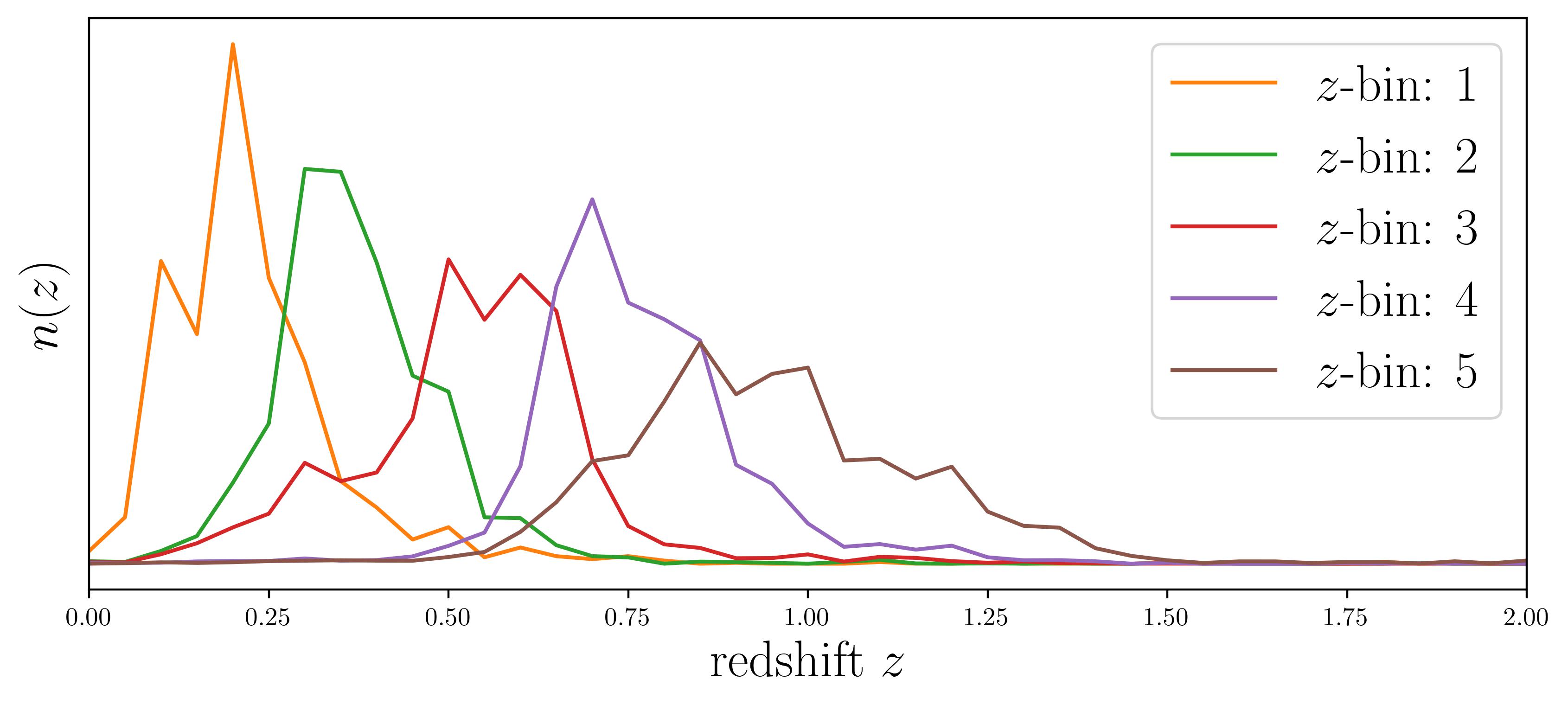
Figure 1: Redshift distribution of the five tomographic redshift bins of the KiDS-1000 data.

The KiDS-1000 cosmic shear catalogue is divided into five tomographic $z$-bins, whose redshifts are calibrated using the self-organising map (SOM) method described in Wright et al. (2020). The redshift distributions of all five tomographic bins are shown in Fig. 1, and were initially presented in H21. The residual systematic uncertainties on the redshift distributions are listed in Table 5 and are included in this work as nuisance parameters which we marginalise over. We note that they are actually correlated, which we account for by using their correlation matrix for the marginalisation. The galaxy shear ellipticities and their corresponding weights $w$ are estimated by the lensfit tool (Miller et al. 2013; Fenech Conti et al. 2017; Kannawadi et al. 2019) and are described in more detail in Giblin et al. (2021). These shear-related systematic effects shift the $S_{8}$ parameter by, at most, $0.1\sigma$ when measured by cosmic shear two-point functions. The resulting systematics are stated in Table 5, where we marginalise over the shear multiplicative $m$-bias correction in the resulting posteriors.

Table 1: Overview of the observational KiDS-1000 data.

name	$n_{\mathrm{eff}}[\mathrm{arcmin}^{-2}]$	$\delta\langle z\rangle$	$\sigma_{\epsilon}$	$m$-bias $\times 10^{3}$
$z$-bin: 1	0.62	$0.000\pm 0.0106$	0.270	$-10\pm 19$
$z$-bin: 2	1.18	$0.002\pm 0.0113$	0.258	$-9\pm 20$
$z$-bin: 3	1.85	$0.013\pm 0.0118$	0.273	$-11\pm 17$
$z$-bin: 4	1.26	$0.011\pm 0.0087$	0.254	$8\pm 12$
$z$-bin: 5	1.31	$-0.006\pm 0.0097$	0.270	$12\pm 10$

5 Simulated data

To validate our inference pipeline, study the impact of key systematic uncertainties, and forecast the expected KiDS-1000 analysis, we use several simulated data sets created to resemble the observed KiDS-1000 data.

In particular, we use the full-sky gravitational lensing simulations described in Takahashi et al. (2017, hereafter T17) to generate data vectors and numerical covariance matrices. The cosmo-SLICS+IA simulations, described in Harnois-Déraps et al. (2022), are used to test the modelling of IA; and the Magneticum lensing simulations, first introduced in Hirschmann et al. (2014), to infuse Baryon feedback on the model which strength we regulate with a free parameters in the posterior estimation.

5.1 Takahashi simulations

Since the T17 simulations are used in this series of previous works, we only repeat the essential details here. The T17 simulations follow the non-linear evolution of $2048^{3}$ particles evolved in a large series of nested cosmological volumes with side length starting at $L=450\,\mathrm{Mpc}/h$ at low redshift, and increasing at higher redshift, resulting in 108 different full-sky realisations. These were produced by the Gadget-3 $N$-body code (Springel 2005) and are publicly available. The cosmological parameters of the matter and vacuum energy density are fixed to $\Omega_{\rm m}=1-\Omega_{\Lambda}=0.279$, the baryon density parameter to $\Omega_{\rm b}=0.046$, the dimensionless Hubble constant to $h=0.7$, the normalisation of the power spectrum to $\sigma_{8}=0.82$, and the spectral index to $n_{\rm s}=0.97$. The shear information of the T17 simulations is given in terms of 108 $\gamma$ and $\kappa$ full-sky realisations, where each realisation is divided into 38 ascending redshift slices. To reproduce the KiDS-1000 data for a given tomographic $z$-bin shown in Fig. 1, we build the weighted average of the first 30 $\gamma$ and $\kappa$ redshift slices. The weight for each redshift slice is measured by integrating the $n(z)$ over the corresponding width of the redshift slice.

We decided on two approaches (convergence maps vs. galaxy ellipticity) to measure the data vectors and covariance matrices from the T17 simulations. While the first approach (Sect. 5.1.1) has the advantage that a large number of mocks is available to measure a reliable covariance matrix even for large data vectors, the second approach (Sect. 5.1.2) has the advantage that the exact galaxy positions are used, which implies that the holes (masks) match the data.

5.1.1 Convergence mocks

The first approach is to convolve the full sky convergence maps with the $T_{\mathrm{\pm,n}}(\theta_{\mathrm{ap}})$ or $U(\theta_{\mathrm{ap}})$ filters, then multiply with corresponding other smoothed maps, and then take the spatial average. For the covariance matrix, we divided the smoothed convergence maps into 48 sub-patches, where each patch has an area of $860\,\mathrm{deg}^{2}$. Since the $\kappa$ maps are first convolved with the filter functions and the sub-patches have common edges the individual patches are not fully independent from each other, which decreases the covariance matrix. However, we have tested that by selecting only 18 sub-patches, which have no common edges give almost identical results. Shape noise is added to the convergence maps by drawing random numbers from a Gaussian distribution with a vanishing mean and a standard deviation

$$\sigma=\frac{\sigma_{\epsilon}}{\sqrt{n_{\mathrm{eff}}\,A_{\mathrm{pix}}}}\;,$$ (35)

with the pixel area $A_{\mathrm{pix}}=0.74\,\mathrm{arcmin}^{2}$ $(\textsc{nside}=4096)$, $n_{\mathrm{eff}}$ the effective galaxy number density that included the lensfit weights, and $\sigma_{\epsilon}$ the shape noise contribution given in Table 5. With 48 sub-patches and 108 realisations, the covariance matrix is measured from 5184 mocks. As the actual KiDS-1000 area is roughly $777.4\,\mathrm{deg}^{2}$, we area rescaled the covariance by $860\,\mathrm{deg}^{2}/777.4\,\mathrm{deg}^{2}\approx 1.1$. The reference data vector is measured from one T17 realisation with a resolution of $A_{\mathrm{pix}}=0.18\,\mathrm{arcmin}^{2}$ $(\textsc{nside}=8192)$ without shape noise.

5.1.2 Galaxy shear catalogue mocks

For real surveys with a complex topology, the convolved maps give biased results (Seitz & Schneider 1997). We, therefore, decided on our second approach to measure our statistics from second- and third-order shear correlation functions. For this, we created galaxy shear catalogues from projected $\gamma$ and $\kappa$ fields by extracting the shear information only at the true positions of the observed galaxies in KiDS-1000. Since the correlation functions need to be measured to very small scales, we used realisations with a pixel resolution of $A_{\mathrm{pix}}=0.18\,\mathrm{arcmin}^{2}$ $(\textsc{nside}=8192)$. We have checked that this resolution is sufficient by comparing the data vectors obtained from catalogs constructed from the same initial conditions on the reference resolution $(\textsc{nside}=8192)$ and a higher resolution $(\textsc{nside}=16384)$, finding a maximum deviation of $1\%$ for an aperture filter scale of $4^{\prime}$. To increase the number of mocks, we shifted the galaxy positions 18 times by $20\mathrm{°}$ along the declination and extracted the shear information at the new positions. Afterwards, the shifted galaxy positions and the corresponding lensing information are shifted back to the original footprint. The back shifting is done only for simplicity and has no physical reason. With this procedure 1944 almost independent mocks are created, from which the covariance and the reference data vector are measured. To add shape noise, we combine the two-component reduced shear $g=\gamma/(1-\kappa)$ of each object with a shape noise contribution $\epsilon^{\mathrm{s}}$ to create observed ellipticities ${\boldsymbol{\epsilon}}^{\mathrm{obs}}$ as (Seitz & Schneider 1997)

$$\epsilon^{\mathrm{obs}}=\frac{{\epsilon}^{\mathrm{s}}+{g}}{1+{\epsilon}^{\mathrm{s}}{g}^{*}}\,.$$ (36)

The quantities here are all complex numbers, and the asterisk ‘$*$’ indicates complex conjugation. To mock the $\epsilon^{\mathrm{s}}$, we use the observed ellipticities $\epsilon_{\mathrm{KiDS}}^{\mathrm{obs}}$ of the KiDS-1000 data and randomly rotate them to erase the underlying correlated shear signal. This procedure has the advantage that the resulting distribution of $\epsilon^{\mathrm{s}}$ matches the distribution of $\epsilon_{\mathrm{KiDS}}^{\mathrm{obs}}$. The estimated mean and dispersion $\sigma_{\epsilon}$ are given in Table 5. Furthermore, when computing our statistics via correlation functions, we need to consider the corresponding weight $w$ for each shape measurement, which ensures that we use the correct effective number density. Since the lensing weights and the intrinsic ellipticities of source galaxies are correlated, adding the rotated ellipticities to the shear signal preserves this correlation.

5.1.3 Data vector measurement and modelling

We follow the analysis of Asgari et al. (2021, hereafter A21) as it is the fiducial cosmic shear analysis of the KiDS-1000. We use only the first five $E_{n}$-moments determined from two-point correlation functions, measured from $0.\mathrm{\prime }5$ to $300\mathrm{\prime }$ in 400 radial bins. The resulting $E_{n}$ are shown in Fig. 2, where we have checked that the $B_{n}$ are consistent with zero. The $E_{n}$ data vector for $\gamma$ and $g$ is the mean of all 1944 T17 mocks, and for $\kappa$ data vector we used one realisation with resolution $A_{\mathrm{pix}}=0.18\,\mathrm{arcmin}^{2}$ $(\textsc{nside}=8192)$. The analytical model is computed using CosmoSIS (Zuntz et al. 2015a).

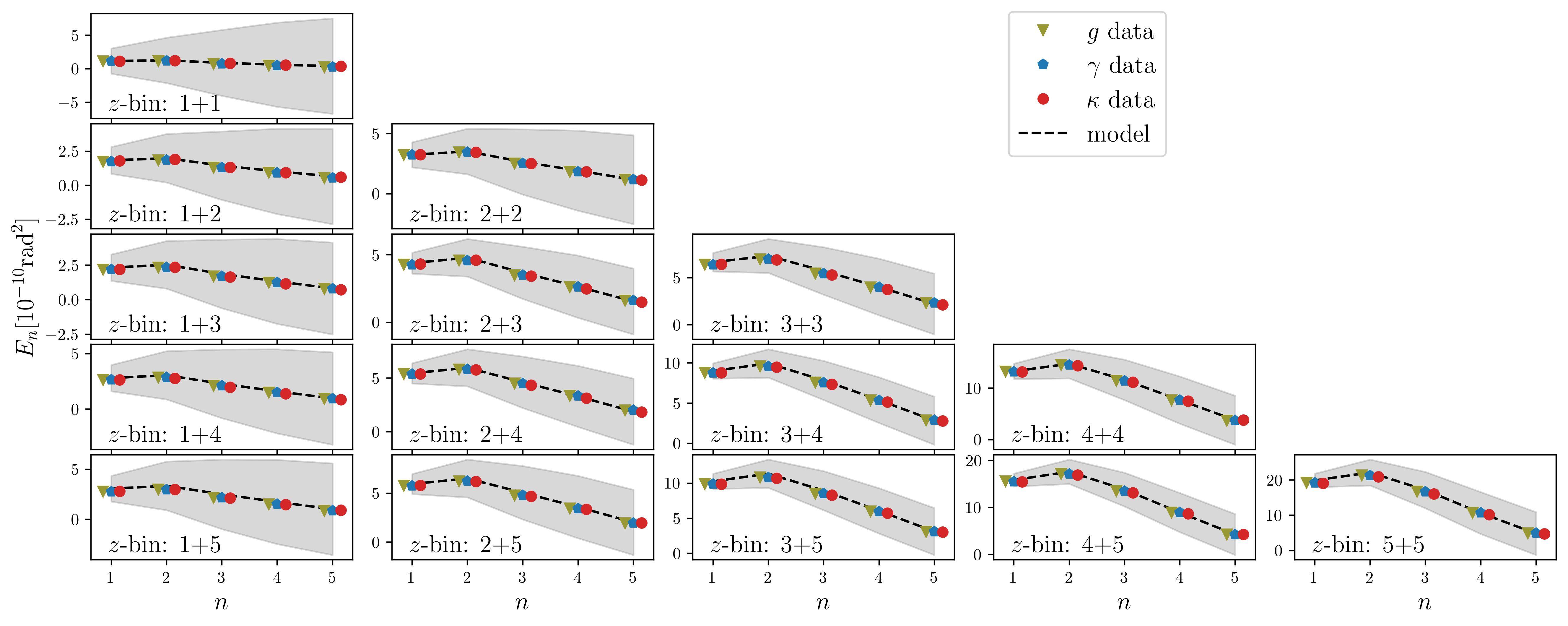
Figure 2: Measured and modelled $E_{n}$ vector for the first five moments in the T17 mocks. The green and blue dots are the mean of all 1944 KiDS-1000 mocks that are also used to compute the covariance matrix with a resolution $A_{\mathrm{pix}}=0.18\,\mathrm{arcmin}^{2}$ and shape noise. The red dots represent the data vector measured from one full-sky T17 realisation with a resolution $A_{\mathrm{pix}}=0.18\,\mathrm{arcmin}^{2}$ and no shape noise. The grey band indicates the expected uncertainty from the KiDS-1000 survey.

The ${\expectationvalue{\mathcal{M}_{\mathrm{ap}}^{3}}}$ data vectors are measured from the same mocks that are also used to compute the $E_{n}$. The analytical model pipeline is described in H23. In Fig. 3, we show ${\expectationvalue{\mathcal{M}_{\mathrm{ap}}^{3}}}$ for aperture filter radii $\theta_{\mathrm{ap}}\in\{$$,$$,$$,$$,$$,$$,$$,$$,$$,$$\}$, where we used only equal scales and show them here for some specific $z$-bin combinations. In 15, we show ${\expectationvalue{\mathcal{M}_{\mathrm{ap}}^{3}}}$ also for non-equal aperture filter radii $\theta_{\mathrm{ap}}\in\{$$,$$,$$,$$\}$.

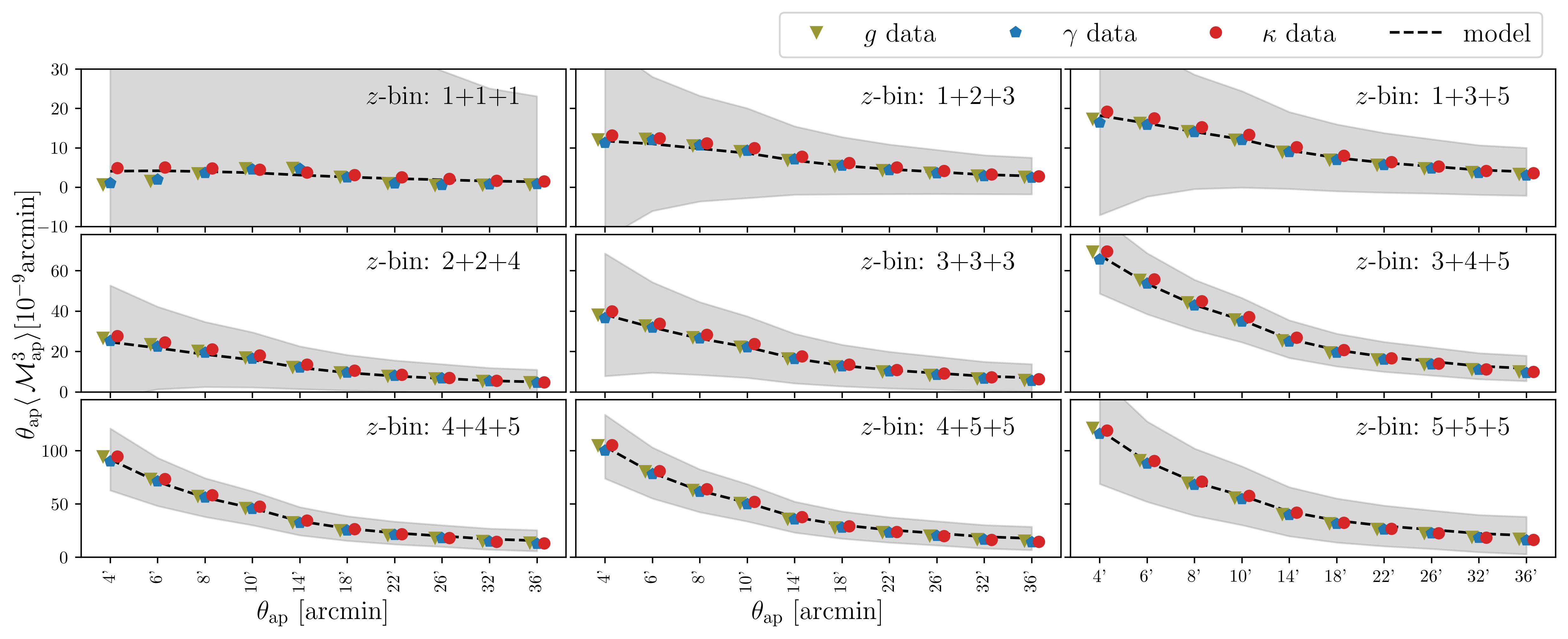
Figure 3: Same as Fig. 2, but here the measured data and model are the ${\expectationvalue{\mathcal{M}_{\mathrm{ap}}^{3}}}$ vector for equal-scale aperture filter radii $\theta_{\mathrm{ap}}\in\{$$,$$,$$,$$,$$,$$,$$,$$,$$,$$\}$ in the T17 mocks for some selected $z$-bin combinations. The full data set is shown in Fig. 14.

5.2 cosmo-SLICS+IA

The cosmo-SLICS+IA simulations are cosmic shear mock galaxy catalogues infused with the non-linear alignment model of Bridle & King (2007), which is ideally suited for testing and validating our analytical IA model. They are based on $N$-body simulations of identical box size and particle density as the SLICS (Harnois-Déraps et al. 2018), which were already used in previous works of this series; we therefore only summarise the essential details.

The cosmology corresponds to the fiducial cosmo-SLICS model presented in Harnois-Déraps et al. (2019), with $\Omega_{\mathrm{m}}=0.2905$, $\Omega_{\Lambda}=0.7095$, $\Omega_{\mathrm{b}}=0.0473$, $h=0.6898$, $\sigma_{8}=0.836$, $w_{0}=-1.0$ and $n_{\rm s}=0.969$. We use the full set of 50 simulated galaxy catalogues, each covering 100 deg² and reproducing the KiDS-1000 $n(z)$ (see Fig. 1) and galaxy number densities $n_{\mathrm{eff}}$ specified in H21. As we use these mocks only to infuse IA effects into the T17 data vector, shape noise is not included. Following the methods described in Harnois-Déraps et al. (2022), the intrinsic ellipticity components $\epsilon_{1/2}^{\rm IA}$ of these galaxies are computed as

$$\epsilon_{1}^{\mathrm{IA}}=-f_{\mathrm{IA}}(\partial_{xx}-\partial_{yy})\phi\;,\quad\epsilon_{2}^{\mathrm{IA}}=-2f_{\mathrm{IA}}\partial_{xy}\phi\,,$$ (37)

where $f_{\mathrm{IA}}$ is defined in Eq. (7), and $\phi$ is the gravitational potential. The partial derivatives of the gravitational potential describe the Cartesian components of the projected tidal field tensors. The $\epsilon_{1/2}^{\rm IA}$ terms are then combined with the noise-free cosmic shear signal using Eq. (36), resulting in an IA-contaminated weak lensing sample that is consistent with the NLA model. As these mocks cover a square patch without any masking, we use the methods described in Sect. 3.2 to estimate the aperture statistics. Furhtermore, they are only used for the validation of the IA modelling, which we perform in Appendix A.

5.3 Magneticum simulations

The feedback processes due to baryonic matter significantly affect the distribution of the LSS, such that the clustering of the matter is reduced on intra-cluster scales by up to tens of per cent (van Daalen et al. 2011). However, quantitatively this suppression is not well understood (Chisari et al. 2015). We use the Magneticum simulations (Hirschmann et al. 2014) to investigate the impact of baryonic feedback processes. Magneticum was run using Gadget3 code which is a more efficient version of Gadget 2 (Springel 2005) that includes modern smoothed particle hydrodynamics (Beck et al. 2016). The dark matter particle mass is $6.9\times 10^{8}h^{-1}M_{\odot}$ and gas particle mass $1.4\times 10^{8}h^{-1}M_{\odot}$. The underlying matter fields are constructed from the Magneticum Pathfinder simulations in the Run-2 with a comoving volume of side $352\,h^{-1}\,{\mathrm{Mpc}}$ and Run-2b with a comoving volume of side $640\,h^{-1}\,{\mathrm{Mpc}}$, and are described in Hirschmann et al. (2014) and Ragagnin et al. (2017), respectively. The Magneticum simulations account for radiative cooling, star formation, supernovae and active galactic nuclei.

The Magneticum shear maps used in this work were first presented in Castro et al. (2018). Although the underlying creation of these shear maps is similar to the production of the cosmo-SLICS, meaning that the mocks follow the same redshift distribution and number density as the KiDS-1000 data, there are three main differences. First, only ten instead of 50 pseudo-independent light cones are available. Second, the galaxies are not randomly placed but at the exact galaxy positions as in the observed data. Third, as these mocks are flat sky simulations and cover only an area of $100\,\mathrm{deg}^{2}$, the KiDS-1000 footprint is divided into 18 regions. This results in 18 catalogues for each of the ten pseudo-independent light cones. Due to the non-trivial geometry of the masks, we used correlation functions to estimate the shear statistics.

To incorporate baryonic feedback processes into our modelling pipeline using the Magneticum simulations, we calculated the data vector $\mathbf{d}^{\mathrm{DM}}$ using dark matter only and the data vector $\mathbf{d}^{\mathrm{DM+BA}}$ where dark matter and baryons are included. With them we modify the model vector $\mathbf{m}$ to

$$\mathbf{m}^{\prime}=\left[1+A_{\mathrm{ba}}\left(\frac{\mathbf{d}^{\mathrm{DM+BA}}}{\mathbf{d}^{\mathrm{DM}}}-1\right)\right]\mathbf{m}\,,$$ (38)

where we introduce the parameter $A_{\mathrm{ba}}$. A value of zero for $A_{\mathrm{ba}}$ means no baryonic feedback and a value of one is exactly the strength of baryonic feedback as in the Magneticum. Furthermore, we interpolate between zero and one and extrapolate to even five, which we arbitrarily chose. We note that the $A_{\mathrm{BA}}$ has no physical meaning and is only introduced to give the model some flexibility to account for baryonic feedback effects.

6 Cosmological parameter inference methodology

In the following sections, we will determine multiple posterior distributions using Markov chain Monte Carlo (MCMC) samplings for different model ingredients.

We vary the two cosmological parameters $\Omega_{\mathrm{m}}$ and $S_{8}$ while fixing the remaining parameters to the T17 cosmology. Additionally, we vary the intrinsic alignment amplitude, $A_{\mathrm{IA}}$, and the parameter $A_{\mathrm{ba}}$ that accounts for the strengths of the response to baryonic feedback and was described in Sect. 5.3. Lastly, we always marginalise over the shifts of the redshift distributions $\delta\langle z\rangle$ given in H21 and the $m$-bias (Giblin et al. 2021) of all five tomographic bins shown in Table 5. For these nuisance parameters, we assume Gaussian priors and account for the fact that the uncertainties of shifts of the redshift distributions are correlated using its correlation matrix. We give an overview of the priors in Table 11.

Table 2: All varied parameters and their flat prior knowledge.

parameter	validation	real
$\Omega_{\mathrm{m}}$	$[0.10,0.50]$	$[0.10,0.75]$
$S_{8}$	$[0.6,1.0]$	$[0.6,1.0]$
$A_{\mathrm{IA}}$	$[-1.8,1.8]$	$[-1.5,1.5]$
$A_{\mathrm{ba}}$	$[0.0,5.0]$	$[0.0,5.0]$

If the covariance matrix $\tilde{C}$ is measured from simulations, it is a random variable. We follow the method of Percival et al. (2022) which leads to credible intervals that can also be interpreted as confidence intervals with approximately the same coverage probability. The posterior distribution of a model vector $\mathbf{m}$ that depends on $n_{p}$ parameters $\boldsymbol{p}$ if the covariance matrix $\tilde{C}$ is measured from $n_{\mathrm{r}}$ mocks, is given by

$$\boldsymbol{P}\left[\mathbf{m}(\boldsymbol{p})|\mathbf{d},\tilde{C}\right]\propto|\tilde{C}|^{-\frac{1}{2}}\left(1+\frac{\chi^{2}}{n_{\rm r}-1}\right)^{-m/2}\,,$$ (39)

where $\mathbf{d}$ is the measured data vector and

$$\chi^{2}=\left[\mathbf{m}(\boldsymbol{p})-\mathbf{d}\right]^{\rm T}\tilde{C}^{-1}\left[\mathbf{m}(\boldsymbol{p})-\mathbf{d}\right]\,.$$ (40)

The power-law index $m$ is

$$m=n_{p}+2+\frac{n_{\mathrm{r}}-1+B(n_{\mathrm{d}}-n_{p})}{1+B(n_{\mathrm{d}}-n_{p})}\;,$$ (41)

with $n_{\rm d}$ being the number of data points and

$$B=\frac{n_{\mathrm{r}}-n_{\mathrm{d}}-2}{(n_{\mathrm{r}}-n_{\mathrm{d}}-1)(n_{\mathrm{r}}-n_{\mathrm{d}}-4)}\,.$$ (42)

To give a quantified value for the comparison of different modelling choices, we use the Figure of Merit (FoM), which we calculate as

$$\mathrm{FoM}=\frac{1}{\sqrt{\det C}}\,,$$ (43)

where $C$ is the parameter covariance matrix of the $S_{8}$-$\Omega_{\mathrm{m}}$ plane resulting from the MCMC process.

Depending on the used filter combinations, the modelling of ${\expectationvalue{\mathcal{M}_{\mathrm{ap}}^{3}}}$ takes around $10$ to $20\,\mathrm{min}$, which prevents running an MCMC using the model directly. To circumvent this issue, we use the emulation tool contained in CosmoPower (Spurio Mancini et al. 2022). We trained the emulator on 3000 model points for the analysis based on mocks in the parameter space $\{\Omega_{\rm m},S_{8},A_{\mathrm{IA}}\}$ and 5000 model points for the real data analysis in the parameter space $\{\Omega_{\rm m},S_{8},A_{\mathrm{IA}},\delta\langle z\rangle\}$, which we distributed in a Latin hypercube for the given prior range, and fixed all other parameters to the ones used in the T17 simulations. The $m$-bias and the $A_{\mathrm{ba}}$ do not need to be emulated as they follow a simple correction formalism that is applied during the MCMC sampling. The $\delta\langle z\rangle$ of each $z$-bin for the training and testing are distributed uncorrelated between $[-0.06,0.06]$. The accuracy of the emulator is tested by comparing the emulator prediction with the model at 500 independent points in the same parameter space. The fractional error of each vector element is smaller than $2\%$ for $E_{n}$ and smaller than $5\%$ for ${\expectationvalue{\mathcal{M}_{\mathrm{ap}}^{3}}}$, which is well within the accuracy of the HMcode2020 or the BiHalofit model itself. We used a Metropolis–Hastings sampler for MCMC, where we used 1000 walkers running each 20 000 steps and cut the first 2000 steps away to ensure that the posteriors are not biased by the burn-in phase.

7 Reduction of data vector combinations and filter radii

Generally, as long as the covariance is converged, the more information is used, the higher the constraining power. However, for third-order statistics with four different filter radii and five tomographic bins, the data vector contains 700 elements. To have a reliable covariance matrix, roughly $\sim 10$ times the dimension of the data vector is needed. This implies that modelling and measuring the model/data vector and covariance matrix are time-consuming and require thousands of simulations. Therefore, it is inevitable for this and for future analyses to compress the data vector without substantial information loss. We note that this section is only concerned with reducing the dimension of the data vector and is not meant as a proper forecast, which we do in the following sections. The spatial resolution of the mocks used to compute the covariance induces an error smaller than $<1\%$ in the $E_{n}$ covariance matrix. However, as we only reduce the elements of ${\expectationvalue{\mathcal{M}_{\mathrm{ap}}^{3}}}$, while using all combinations of the $E_{n}$, this is unproblematic for the purpose of this section. We note again that the data vector is measured from one realisation with a of resolution of $A_{\mathrm{pix}}=0.18\,\mathrm{arcmin}^{2}$, and that we use the $\kappa$ based covariance for this section to ensure the covariance matrix is converged even for the data vector with the largest dimension. As a first check, we show in Fig. 4 multiple element choices that discard a significant part of the ${\expectationvalue{\mathcal{M}_{\mathrm{ap}}^{3}}}$ data vector. Using only the five auto-tomographic bins is not a good choice for reduction as seen in the fact that the FoM reduced by $32\%$. However, using only equal-scale aperture radii is a better reduction, reducing the data vector to $28\%$ while reducing the FoM by only $\approx 8\%$. Using only equal-scale aperture radii also has the advantage of being modelled faster. Therefore, we continue using only the equal-scale aperture radii for the rest of this work, which reduces the dimension of the data vector from 775 to 215.

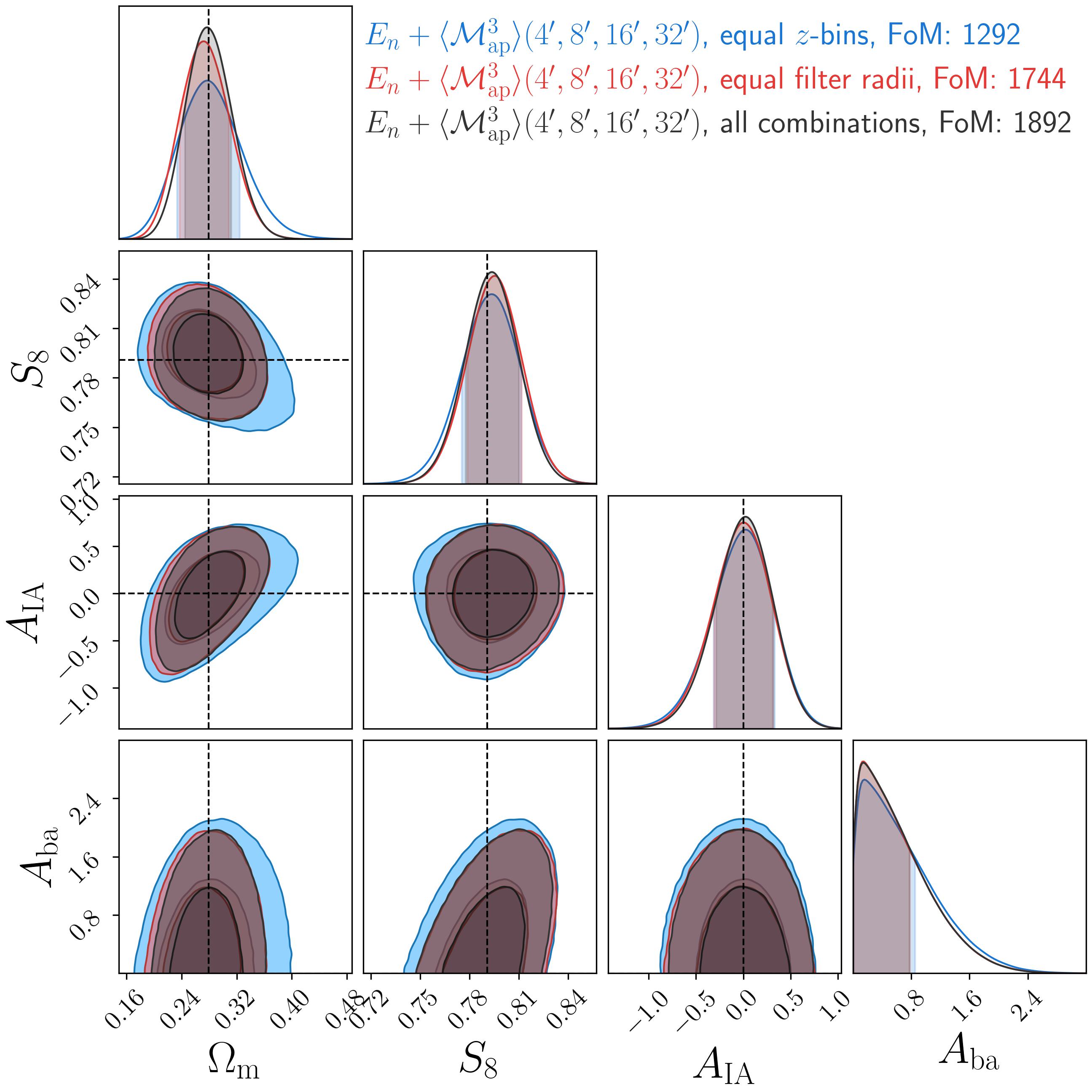
Figure 4: Posterior distribution for data vectors and covariance measured from the T17 convergence maps catalogues. Here only specific parts of the ${\expectationvalue{\mathcal{M}_{\mathrm{ap}}^{3}}}$ data vector are used. Here ‘only equal $z$-bins’ mean that only the auto tomographic bins are used. Lastly, all non-equal filter radii are discarded for ‘only equal filter radii’.

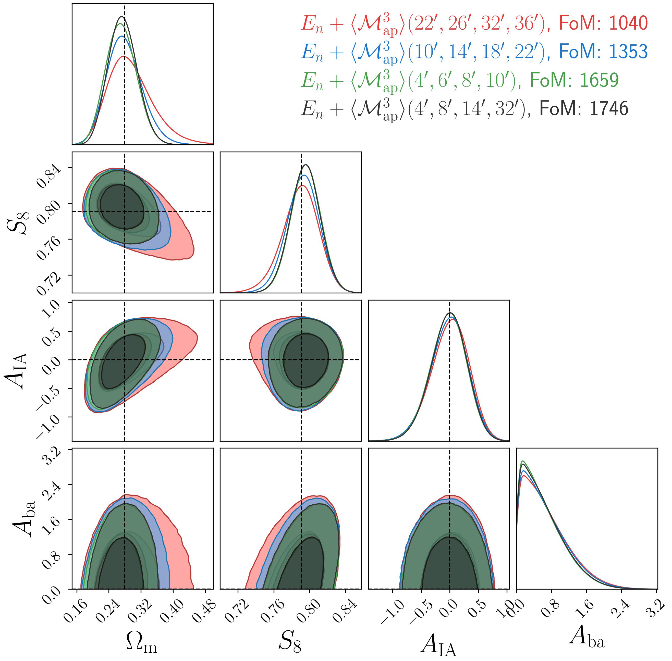
Figure 5: Posterior distribution for different filter radii combinations if the data vector and covariances are measured from the T17 convergence maps.

Next, we investigated the choice of aperture filter radii. The aperture filter radii under consideration are $\theta_{\mathrm{ap}}\in\{$$,$$,$$,$$,$$,$$,$$,$$,$$,$$\}$. The resulting posteriors are displayed in Fig. 5, which reveals that using only the large filter radii above $>$$$ have the worst constraining power. However, using only the four smallest filter radii is also not the best choice, as they are largely correlated and miss the large-scale information. The best choice of filter function is to use a filter from each range like $\theta_{\mathrm{ap}}\in\{$$,$$,$$,$$\}$.

Table 3: Overview of the ${\expectationvalue{\mathcal{M}_{\mathrm{ap}}^{3}}}$ data vector choices and their relative constraining power.

choice	Figure	rel. FoM	$n_{d}$
all combinations	4	1.00	775
only equal $z$-bins	4	0.68	175
$\theta_{\mathrm{ap}}\in\{$$,$$,$$,$$\}$	4	0.92	215
$\theta_{\mathrm{ap}}\in\{$$,$$,$$,$$\}$	5	0.92	215
$\theta_{\mathrm{ap}}\in\{$$,$$\}$	-	0.87	145
$\theta_{\mathrm{ap}}\in\{$$,$$,$$\}$	-	0.89	180
$\theta_{\mathrm{ap}}\in\{$$,$$,$$,$$\}$	5	0.88	215
$\theta_{\mathrm{ap}}\in\{$$,$$,$$,$$\}$	5	0.72	215
$\theta_{\mathrm{ap}}\in\{$$,$$,$$,$$\}$	5	0.55	215
all equal-filter radii	-	0.92	425
best 100 elements	-	0.80	100
best 215 elements	-	0.89	200

Next, we consider the full data vector meaning the ${\expectationvalue{\mathcal{M}_{\mathrm{ap}}^{3}}}$, and the $E_{n}$ for the next compression strategy. The idea is to decrease the number of elements by considering only those with the highest constraining power on $S_{8}$. We start with the element with the highest $S/N$, then consecutively add those vector elements that maximise the $S_{8}$ Fisher information content. This Fisher information is calculated as (Tegmark et al. 1997)

$$F_{S_{8}}=\left(\frac{\partial\boldsymbol{m}(S_{8})}{\partial S_{8}}\right)^{T}C^{-1}\left(\frac{\partial\boldsymbol{m}(S_{8})}{\partial S_{8}}\right)\;,$$ (44)

where the partial derivatives are computed with a five-point stencil beam (Fornberg 1988),

$$\frac{\partial\boldsymbol{m}(S_{8})}{\partial S_{8}}\approx\frac{-\boldsymbol{m}(S_{8}^{++})+8\boldsymbol{m}(S_{8}^{+})-8\boldsymbol{m}(S_{8}^{-})+\boldsymbol{m}(S_{8}^{--})}{12\Delta S_{8}}\;,$$ (45)

where $S_{8}^{\pm}=S_{8}^{\mathrm{T17}}\pm 0.02\,S_{8}^{\mathrm{T17}}$ and $S_{8}^{\pm\pm}=S_{8}^{\mathrm{T17}}\pm 0.04\,S_{8}^{\mathrm{T17}}$. For this analysis, we used only the equal-scale filter radii $\theta_{\mathrm{ap}}\in\{$$,$$,$$,$$,$$,$$,$$,$$,$$,$$\}$. The first $\sim 200$ elements are sufficient to get converged posteriors. It is also interesting to see which elements help increase the constraining power. Obviously, the first elements are all COSEBIs, but among the first 100, approximately half are ${\expectationvalue{\mathcal{M}_{\mathrm{ap}}^{3}}}$ elements. Furthermore, it is interesting to see that cross-tomographic bin elements are more likely to be selected by our method, which is expected because they have a higher $S/N$ than auto-tomographic bin elements. Nevertheless, we also observe that using equal-scale filter radii $\theta_{\mathrm{ap}}\in\{$$,$$,$$,$$\}$ results in a better FoM then using the best 215 elements. This is likely because we optimised here only the $S_{8}$ parameter while fixing all others. Therefore, we also checked for the equal scale filter case if a principal component analysis (PCA) applied to the covariance matrix performs better in compressing the data. However, it needs even more elements to get the same constraining power as our FoM maximiser. This is probably because a PCA considers only the covariance matrix and ignores the derivatives, meaning that a PCA is not necessarily sensitive to cosmology.

Finally, we give in Table 13 an overview of the FoM for the $\Omega_{\mathrm{m}}$–$S_{8}$ plane and the size of the data vector for some more element choices. As the covariance matrix is measured from 5184 mocks, we can assume that for all data vector dimensions under consideration, the covariance matrix is converged. Nevertheless, for the next sections, we use the covariance matrix measured from 1944 galaxy shear catalogues, limiting us to a maximum dimension of our data vector $\sim 200$ elements. Given the investigations in this section, we restrict the further sections, to the case where use all $E_{n}$ elements and all ${\expectationvalue{\mathcal{M}_{\mathrm{ap}}^{3}}}$ elements with the equal-scale filter radii $\theta_{\mathrm{ap}}\in\{$$,$$,$$,$$\}$, as this resulted in the best FoM for the restricted dimension of the data vector.

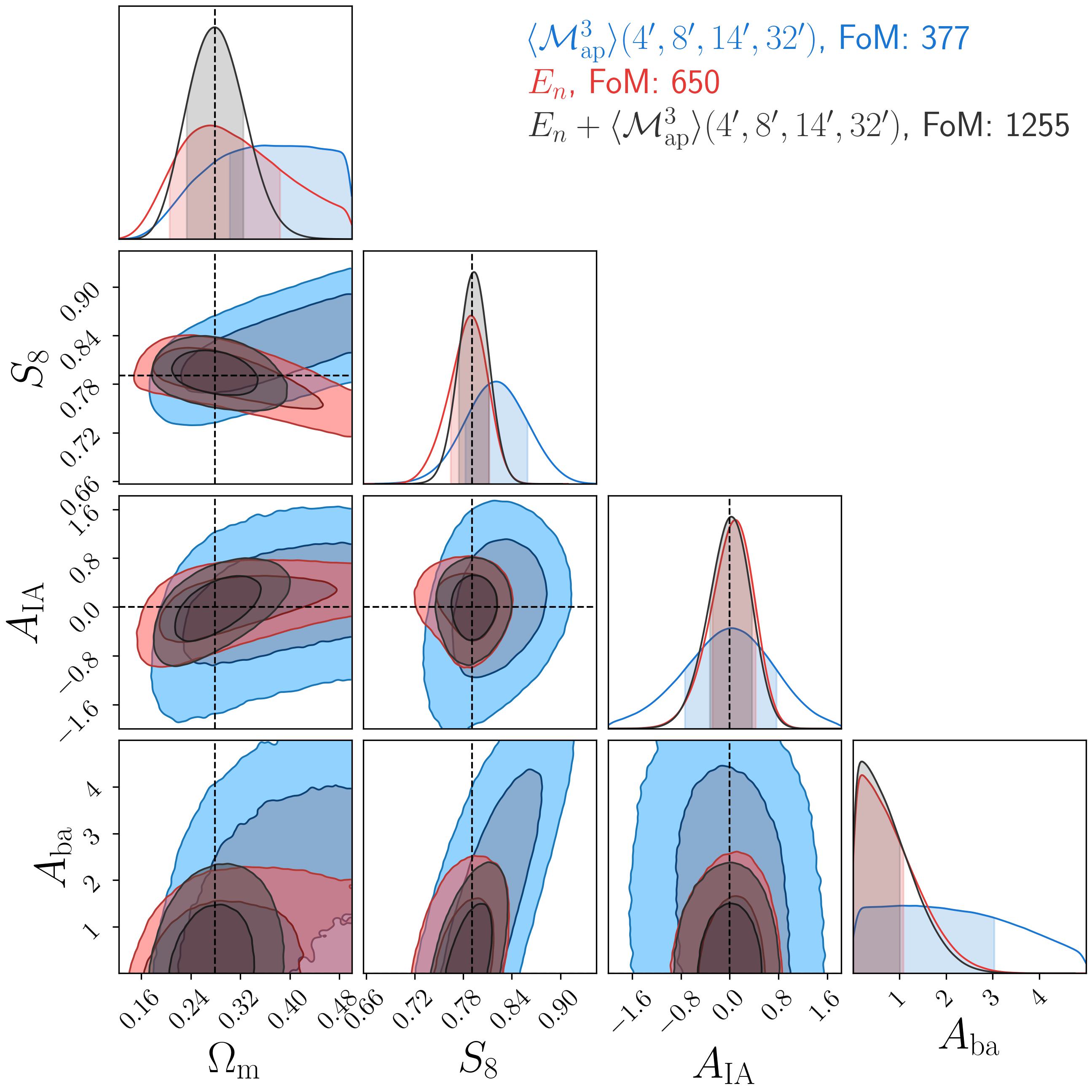
Figure 6: Posterior distribution for data vectors and covariance measured from the T17 galaxy shear catalogues. The covariance matrix and reference data vector are measured from 1944 noisy $g$ mocks.

8 Validation of data vector estimator

In a real survey analysis, two further difficulties arise. The first issue is that the lensing information is not given in terms of convergence maps but by point estimates (galaxies). The finite area where galaxies are measured implies that no lensing information is available outside that area. It is, therefore, necessary to measure the statistic from correlation functions described in Sect. 3.3. Second, these point estimates are the reduced shear $g=\gamma/(1-\kappa)$, which increases the signal and therefore needs to be accounted for. To correct these effects, we measured data vectors without shape noise and with the largest available resolution $A_{\mathrm{pix}}=0.05\,\mathrm{arcmin}^{2}$. Since these data vectors result only from one realisation without shape noise, we can expect that the ratio is a good approximation for the reduced shear effect. Although the deviations are small as seen in Fig. 12 and Fig. 13, we decided to scale the model vectors by the ratio of $g$ and $\gamma$ data vector.

The resulting posteriors are shown in Fig. 6. Our first observation is that similar to the finding of H23, combining second-order with third-order shear statistics significantly improves the constraining power on $S_{8}$ and $\Omega_{\mathrm{m}}$. Compared to the $E_{n}$-only, the $S_{8}$-$\Omega_{\mathrm{m}}$ FoM increases by $93\%$ and for the ${\expectationvalue{\mathcal{M}_{\mathrm{ap}}^{3}}}$-only by even $233\%$. For these improvements, we have not considered that the posteriors of the individual statistics are bound by the priors on $\Omega_{\mathrm{m}}$, meaning that the improvements are lower bounds. Compared to the analysis based on $\kappa$ mocks (see Fig. 5), the posteriors are broader, because the covariance based on $\kappa$ maps also uses information outside the patches since the boundaries are not removed. This decreases the variance between the patches. A further difference is that the $\kappa$ analysis is not subject to masks and uses a slightly larger effective area. Although we rescale the covariance to correct for the different effective areas, we find in Linke et al. (2023) that this rescaling is not necessarily accurate. Lastly, we notice that our modelling within the KiDS-1000 uncertainty is accurate, which we quantify by measuring the shift of the maximum-a-posterior (MAP) from the true values in the matter density parameter $\Delta\Omega_{\mathrm{m}}<0.02\,\sigma_{\Omega_{\mathrm{m}}}$ and in the clustering amplitude $\Delta S_{8}<0.05\,\sigma_{S_{8}}$ with respect to the averaged noisy mock data vector and the KiDS-1000 uncertainty. We define the MAP as the maximum of the one-dimensional marginal distributions.

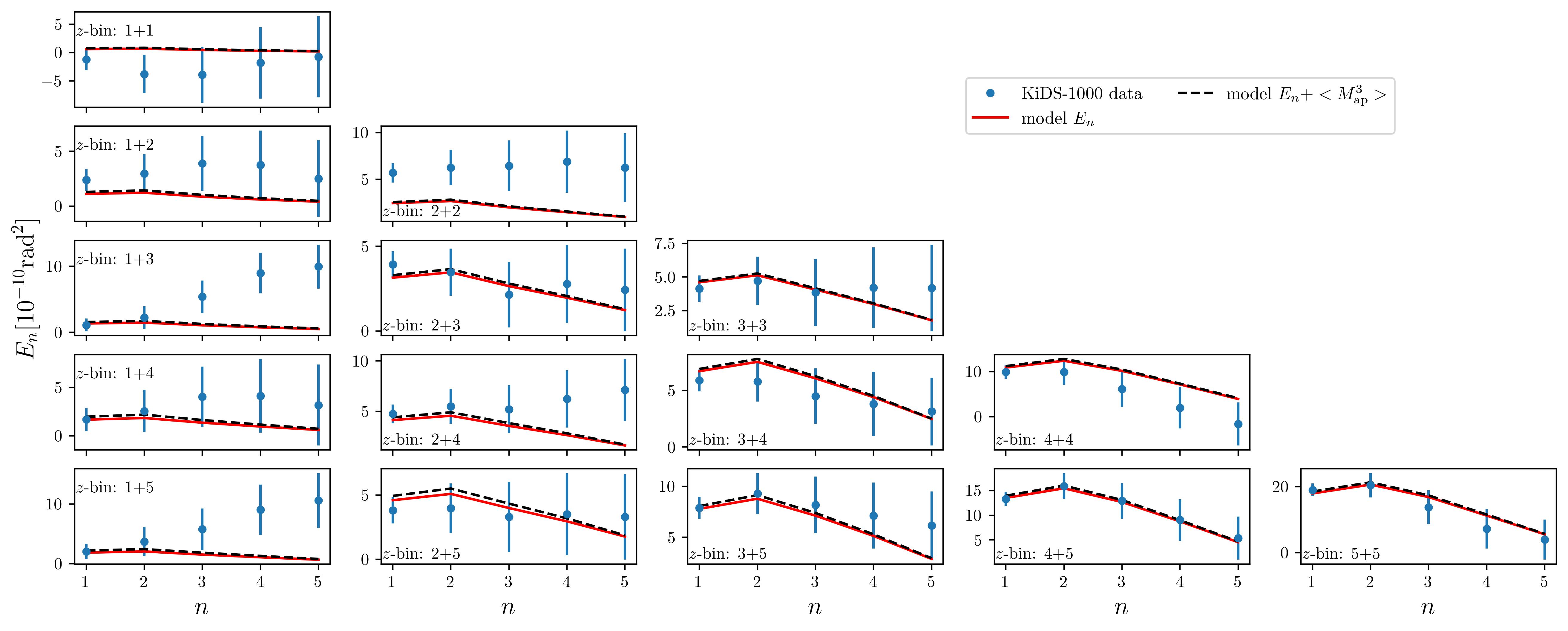
Figure 7: Measured and modelled $E_{n}$ for the first five components. The blue points show the measurements from the KiDS-1000 data A21. The blue error bars indicate the KiDS-1000 uncertainty. The different dashed lines show analytical descriptions at the MAP if the combination of $E_{n}+{\expectationvalue{\mathcal{M}_{\mathrm{ap}}^{3}}}$ or only $E_{n}$ is used.

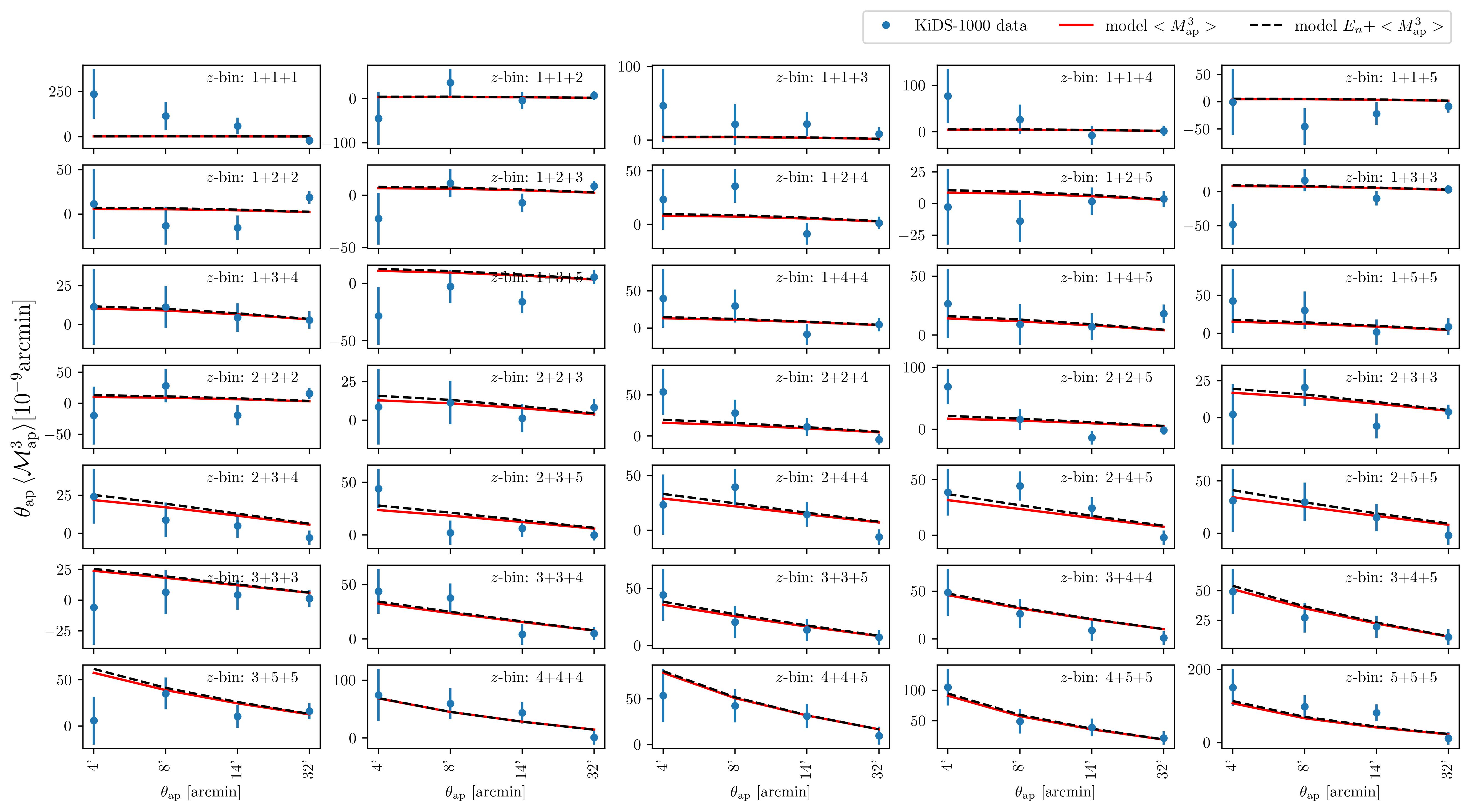
Figure 8: Measured and modelled ${\expectationvalue{\mathcal{M}_{\mathrm{ap}}^{3}}}$ with filter radii $\theta_{\mathrm{ap}}\in\{$$,$$,$$,$$\}$. The blue error bars indicate the KiDS-1000 uncertainty. The different dashed lines show analytical descriptions at the MAP if the combination of $E_{n}+{\expectationvalue{\mathcal{M}_{\mathrm{ap}}^{3}}}$ or only ${\expectationvalue{\mathcal{M}_{\mathrm{ap}}^{3}}}$ is used.

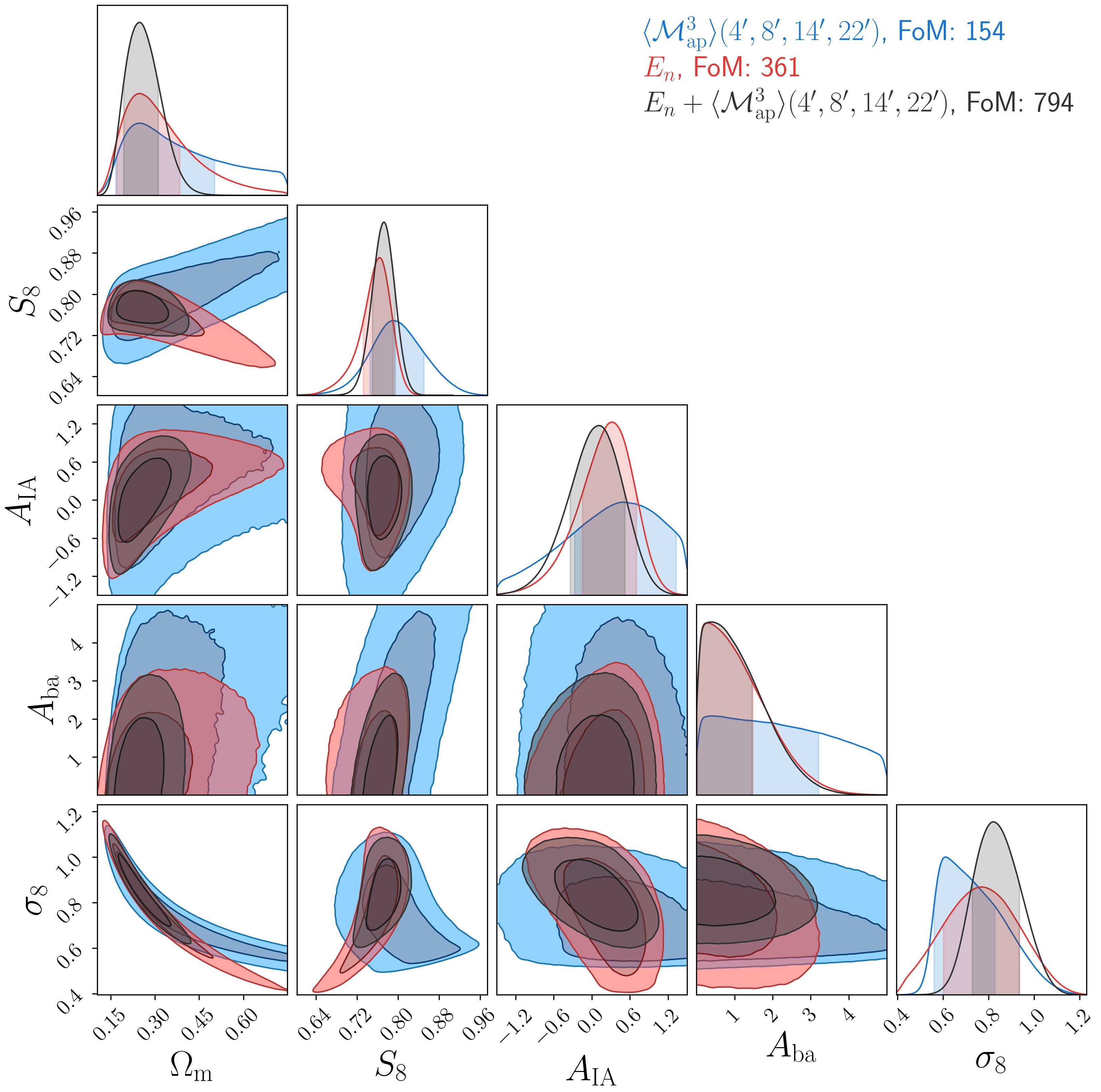
Figure 9: Posterior distribution for the real KiDS-1000 data vector while the covariance is measured from the 1944 T17 galaxy shear catalogues. Here the $E_{n}$ are compared to ${\expectationvalue{\mathcal{M}_{\mathrm{ap}}^{3}}}$ using all available combinations for the aperture filter radii $\theta_{\mathrm{ap}}\in\{$$,$$,$$,$$\}$ and redshift bin combinations. We note that the prior (see Table 11) range on $\Omega_{\mathrm{m}}$ is enlarged compared to the previous validation plots. The FoM values of the $E_{n}$-only or ${\expectationvalue{\mathcal{M}_{\mathrm{ap}}^{3}}}$-only case should not be compared to Fig. 6, as priors of $\Omega_{\mathrm{m}}$ bind their contours.

9 Cosmological results

Finally, we are ready to present the first cosmological constraints from the KiDS-1000 data using second- and third-order shear statistics, displayed in Fig. 7 and Fig. 8. The data vectors are described in more detail in A21 for the $E_{n}$, and the ${\expectationvalue{\mathcal{M}_{\mathrm{ap}}^{3}}}$ in Porth et al. (2023). Given the fact that the covariance matrix is measured only from 1944 realisations using the reduced shear $g$, we decide to build our data and model vector from all $E_{n}$ modes and ${\expectationvalue{\mathcal{M}_{\mathrm{ap}}^{3}}}$ with all equal filter radii $\theta_{\mathrm{ap}}\in\{$$,$$,$$,$$\}$. To control if the model accurately fits the data, we minimise the $\chi_{\mathrm{real}}^{2}$ from the real data and the $\chi_{\mathrm{T17}}^{2}$ from each of the 1944 T17 mocks used to compute the covariance matrix. To estimate the probability of measuring a $\chi^{2}>\chi_{\mathrm{real}}^{2}$ ($p$-value), we count the number of $\chi_{\mathrm{T17}}^{2}$ that are greater than $\chi_{\mathrm{real}}^{2}$ divided by 1944. The resulting $p$-value for the $E_{n}$-only, the ${\expectationvalue{\mathcal{M}_{\mathrm{ap}}^{3}}}$-only, and the combination are given in Table 14. For all combinations, the resulting $p$-values are better than 0.1, indicating that our covariance is well matched to the observed data and our model is accurate enough to describe the data. Our maximum posterior $\chi^{2}$ value increases to 81 if we swap our $E_{n}$ covariance matrix to the analytical expression in Joachimi et al. (2021) calculated at the MAP parameter values in A21. This is unsurprising as the numerical covariance is computed at the T17 cosmology, giving a signal larger than the signal computed at the MAP of A21. Furthermore, our covariance matrix is measured from reduced shear mocks that slightly increase the covariance matrix.

Table 4: MAP values with their marginal $68\%$ credible intervals.

	$\Omega_{\mathrm{m}}$	$S_{8}$	$\sigma_{8}$	$A_{\mathrm{IA}}$	$A_{\mathrm{ba}}$	$\chi^{2}$	$p$-value
$E_{n}$-only	$0.246^{+0.137}_{-0.076}$	$0.765^{+0.025}_{-0.032}$	$0.77^{+0.17}_{-0.16}$	$0.31^{+0.39}_{-0.46}$	$0.19^{+1.29}_{-0.18}$	$72$	$0.42$
${\expectationvalue{\mathcal{M}_{\mathrm{ap}}^{3}}}$-only	$0.248^{+0.253}_{-0.082}$	$0.791^{+0.060}_{-0.046}$	$0.61^{+0.22}_{-0.05}$	$0.49^{+0.83}_{-0.76}$	$0.39^{+2.83}_{-0.38}$	$147$	$0.25$
$E_{n}+{\expectationvalue{\mathcal{M}_{\mathrm{ap}}^{3}}}$	$0.248^{+0.062}_{-0.055}$	$0.772\pm 0.022$	$0.82^{+0.12}_{-0.09}$	$0.12^{+0.40}_{-0.46}$	$0.38^{+1.07}_{-0.37}$	$224$	$0.26$

Next, we show the resulting posteriors in Fig. 9, where we marginalise over the shift in the redshift distribution and multiplicative shear correction, both stated in Table 5. We improve the constraints on $S_{8}$ by $23\%$ and on $\Omega_{\mathrm{m}}$ by even $47\%$ compared to the $E_{n}$-only case. This shows how powerful a combined analysis of the second- and third-order shear statistics is. The constraints on $A_{\mathrm{IA}}$ and $A_{\mathrm{ba}}$ are basically untouched, showing that ${\expectationvalue{\mathcal{M}_{\mathrm{ap}}^{3}}}$ is not helpful for constraining these nuisance parameters.

Compared to the maximum of the one-dimensional marginal distributions constraints of $E_{n}$ measurements given in A21 ($S_{8}=0.758^{+0.017}_{-0.026}$ and $\Omega_{\mathrm{m}}=0.253^{+0.088}_{-0.074}$), we have slightly larger constraints when using only the $E_{n}$. This is because we use a numerical covariance which is larger than the analytical one due to the underlying cosmology and the fact that we model the reduced shear effect. Furthermore, we note that A21 varied $\Omega_{\mathrm{cdm}}h^{2}$, $\Omega_{\mathrm{b}}h^{2}$ and $h$, while we fixed $h$ and $\Omega_{\mathrm{b}}$ and varied only $\Omega_{\mathrm{m}}$. We also find that if we use the same pipeline as A21 but allow larger $\Omega_{\mathrm{cdm}}h^{2}$, the posteriors increase towards larger $\Omega_{\mathrm{m}}$ and therefore get more consistent with our results. Furthermore, we use a different sampler compared to A21 and different baryon feedback process modelling. Nevertheless, our results from the $E_{n}$ analysis are consistent with A21 within $0.03\,\sigma$ in $\Omega_{\mathrm{m}}$ and within $0.14\,\sigma$ in $S_{8}$. Similar to A21, we also perform an internal consistency check, removing one $z$-bin at a time and finding consistent results. We discuss this in more detail in Appendix A and find that, as expected, the fifth $z$-bin is most important to constrain $\Omega_{\mathrm{m}}$ and $S_{8}$. We further discuss in Appendix A modelling checks regarding the infusion of IA, baryon feedback and the reduced shear correction. We find that the baryon feedback and reduced shear corrections are always sub-dominant compared to a shift in $S_{8}$. The IA, however, is important, especially if lower $z$-bins are included, and must be accurately modelled.

Finally, we notice that all statistics are consistent with $A_{\mathrm{IA}}=0$, although both statistics alone seem to favour positive $A_{\mathrm{IA}}$. Interestingly, the joint analysis is shifted to lower $A_{\mathrm{IA}}$ and is slightly more constraining, which we do not observe in the validation in Sect. 8 where all posteriors accurately peak at the input value and all constraining power comes from the $E_{n}$. This might indicate that for real data with non-zero $A_{\mathrm{IA}}$, third-order shear statistics can contribute (at least a bit) to constraining IA, in line with predictions by, e.g. Pyne & Joachimi (2021) or Troxel & Ishak (2012). Furthermore, we see that with our statistic, the baryonic parameter can be confined to $A_{\mathrm{ba}}<1.4$ at $68\%$ confidence. Here we should note, that ${\expectationvalue{\mathcal{M}_{\mathrm{ap}}^{3}}}$ does not help in constraining $A_{\mathrm{ba}}$, which is probably due to the fact that all $A_{\mathrm{ba}}$ effects are absorbed by changes in $S_{8}$.

10 Conclusions

This work validates the combined modelling of second- and third-order shear statistics, showing that its accuracy is well-suited for a KiDS-1000 analysis. Our second-order shear statistic of choice is the $E_{n}$-modes of the COSEBIs (Schneider et al. 2010), and the third-order statistic is ${\expectationvalue{\mathcal{M}_{\mathrm{ap}}^{3}}}$ (Schneider et al. 2005). In particular, we incorporate intrinsic alignment modelling based on the non-linear alignment model of Bridle & King (2007) and validate its accuracy against simulations infused with IA effects. This test is also interesting for other simulation-based analyses for which IA can not be modelled analytically. We incorporate the impact of the baryonic feedback process by measuring a response function using the Magneticum simulations. Since the amplitude of this response function has no physical meaning, it is considered a nuisance parameter, which does not bias our cosmological parameter predictions.

We investigate which parts of the data vector can be neglected without losing too much cosmological information. This is important because the data vector for third-order shear statistics, due to its possibility of combining three different filters with three different redshift bins, inflates the data vector easily to several hundred elements. Therefore, both a numerical and an analytical covariance are difficult to compute. We find that cross-tomographic redshift bins contain a large amount of cosmological information. Using only equal-scale filter radii but all available tomographic bin combinations was the best data compression strategy, which comes with the advantage that equal-scale filters are faster to compute analytically as they require a lower integral accuracy. Next, we investigate the chosen filter radii. For this we measure and model the ${\expectationvalue{\mathcal{M}_{\mathrm{ap}}^{3}}}$ for $\theta_{\mathrm{ap}}\in\{$$,$$,$$,$$,$$,$$,$$,$$,$$,$$\}$. We find that filter radii above $30\mathrm{\prime }$ do not contribute much constraining power and that having many small filter radii is unnecessary. The best option is to use a filter radii from each range like $\theta_{\mathrm{ap}}\in\{$$,$$,$$,$$\}$. We also test if selecting elements that maximise the Fisher information matrix on $S_{8}$ is more optimal, but find no difference in selecting all equal-scale filter radii. However, this method can be used to speed up the modelling and measurement of future analyses by discarding irrelevant elements.

Next, we validate that the correlation function estimator gives accurate results. This is important as, for real data, only correlation function estimators have the potential to give unbiased results. We use realistic mock data, created from the T17 simulations. In particular, we create several galaxy catalogues where the positions of the galaxies are exactly at the KiDS-1000 galaxy positions. We have to rely on correlation functions to measure the second- and third-order statistics, which give unbiased results also if the data has a complex topology. Our first finding is that our modelling and measurement result in unbiased cosmological parameters given the KiDS-1000 uncertainty. Second, we find that using the reduced shear, or the shear itself, does not change the results and can therefore be ignored for the KiDS-1000 data analysis.

We finalise this paper by analysing the real KiDS-1000 data. Our $E_{n}$ constraints are less informative than the original KiDS-1000 analysis. This is mostly because we use a numerical covariance matrix from T17 simulations. But also, the chosen sampler, priors on the cosmological parameters, and the modelling strategy of the baryonic feedback processes impact our constraints. We find an $S_{8}=0.772\pm 0.022$ and an $\Omega_{\mathrm{m}}=0.248^{+0.062}_{-0.055}$, which are improved compared to the $E_{n}$-only case by $23\%$ and by $47\%$, respectively. With a $p$-value of 0.25 we also find a good agreement of model and data given the KiDS-1000 uncertainty. This demonstrates that combining second- and third-order statistics is powerful in constraining cosmological parameters. The gain in constraining power in $\Omega_{\mathrm{m}}$ is also interesting for combined weak lensing and galaxy clustering analysis because the constraining power in $\Omega_{\mathrm{m}}$ for clustering analysis comes with the issue of further nuisance parameters like galaxy bias. However, since second- and third-order shear statistics constrain $\Omega_{\mathrm{m}}$ quite well, combining it with clustering statistics might enable us to learn more about these nuisance parameters.

For future analysis, we leave the optimisation of the IA and baryonic feedback modelling. Especially interesting would be a more physically motivated description of the baryon feedback processes, which are identical for power and bispectrum. As all baryon feedback models rely on hydro simulations, we have to use the same simulations for power and bispectrum. Furthermore, although we found that the reduced shear and limber approximation is sufficient for a KiDS-1000 analysis we probably have to model these effects for future Stage IV surveys. Lastly, we ignore the effect of source clustering for this work. Although Gatti et al. (2023) found it to be relevant for third-order weak lensing statistics based on convergence mass maps, we expect it to be less important for our analysis, which uses shear catalogues and no mass map reconstruction. For future Stage IV surveys, this needs to be investigated.

Appendix A Consistency checks and modelling choices

As a first consistency check, we again inferred the joint analysis posteriors but removed one $z$-bin at a time. The results are shown in Fig. 10 and reveal, most importantly, that all $z$-bins are internally consistent with each other. However, we further observe that $z$-bin one and $z$-bin two are not important for inferring cosmological parameters, as expected, given their S/N as shown in Porth et al. (2023). For the $A_{\mathrm{IA}}$ parameter, in turn, $z$-bin one is very important, as the low redshift is most sensitive to IA. Next, we observe that the third $z$-bin results are basically the same as for all five $z$-bins, meaning that the third bin can eventually be discarded in future KiDS analyses if the dimension needs to be decreased further. Lastly, if either the fourth or fifth $z$-bin is removed, the constraining power on $\Omega_{\mathrm{m}}$ and $S_{8}$ drastically decreases. For the fifth $z$-bin, this also affects the constraining power on $A_{\mathrm{IA}}$.

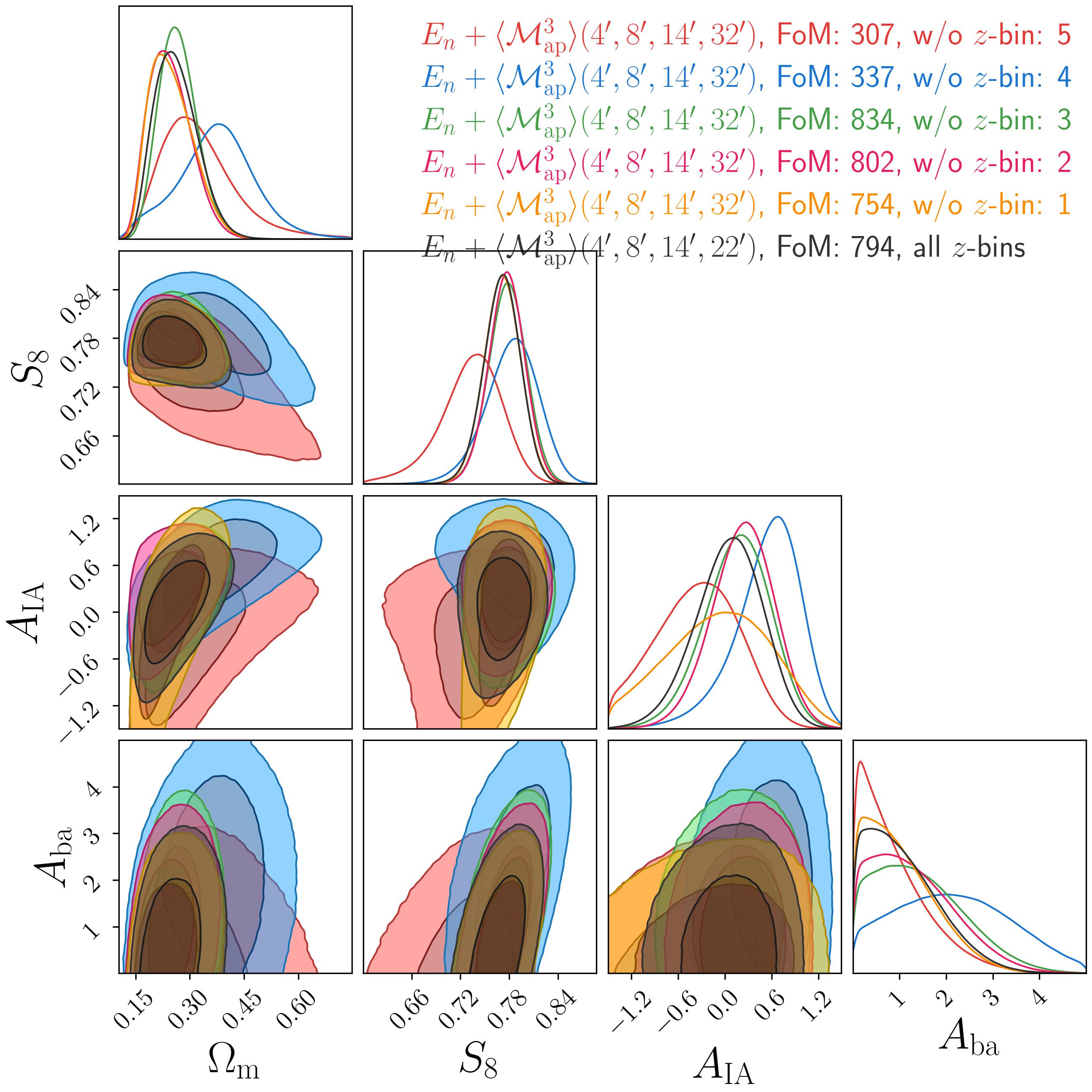
Figure 10: Same as black contours in Fig. 9 but removing one $z$-bin at a time.

Now we investigate the accuracy of the modelling strategy of IA described in Sect. 2.2. To validate our IA modelling, we measured the data vector from the cosmo-SLICS+IA for $A_{\mathrm{IA}}=\{-1,0,1\}$ and then took the ratio of the data vector at $A_{\mathrm{IA}}\in\{-1,1\}$ and divided it by the data vector at $A_{\mathrm{IA}}=0$. This ratio is multiplied with the averaged T17 $\gamma$ mock data vector to infuse IA. For this analysis, we used only equal-scale filter radii $\theta_{\mathrm{ap}}\in\{$$,$$,$$,$$\}$. As seen in Fig. 11, our model nicely recovers the input IA amplitude without shifting the other parameter posteriors. Interestingly, the larger $A_{\mathrm{IA}}$ the larger the FoM, which is due to the increased degeneracy breaking seen in the $\Omega_{\mathrm{m}}$-$A_{\mathrm{IA}}$ panel.

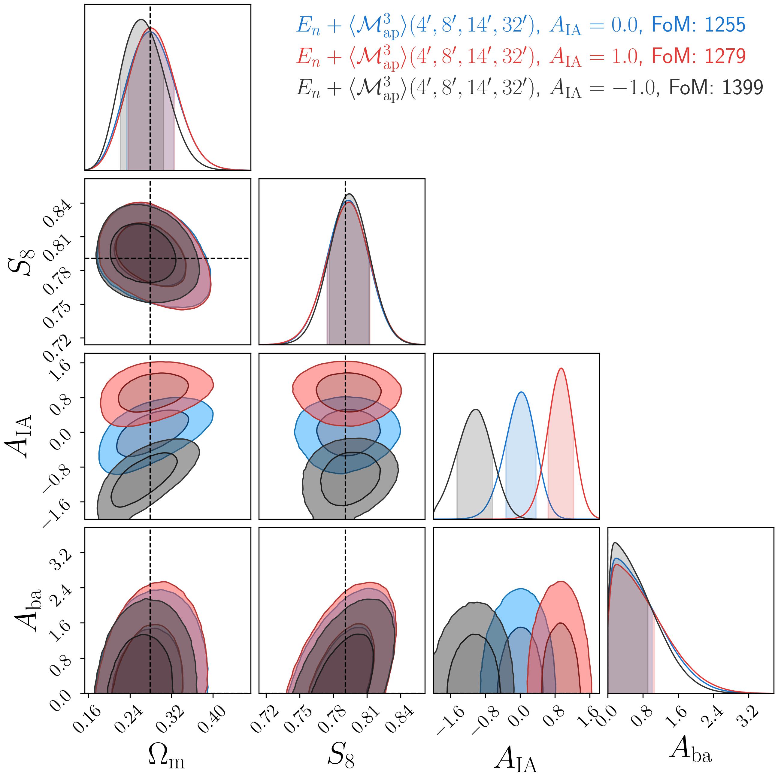
Figure 11: Posterior distribution for data vectors and covariance measured from the 1944 T17 noisy $g$ mocks. Here the T17 data vector is infused with IA measured from the cosmo-SLICS+IA. The modelling is described in Sect. 2.2.

As a further modelling check, we investigate in Fig. 12 and Fig. 13 the impact on our model vector of several ingredients, namely the reduced shear correction, the infusion of baryonic feedback processes and intrinsic alignments (IA). As a reference, we always use a model without reduced shear, $A_{\mathrm{IA}}=0$, $A_{\mathrm{ba}}=0$, $S_{8}=0.78$ and $\Omega_{\mathrm{m}}=0.25$. We then only change one of these effects, while fixing the others. We also show the impact on the model vector if we change the cosmology to $S_{8}=0.8$. The change of the model vectors is divided by the square root of the covariance diagonal, indicating the relevant importance given the KiDS-1000 uncertainty. The reduced shear and baryon feedback correction are always subdominant compared to the impact of $S_{8}$ or IA. For the higher $z$-bins, the $S_{8}$ change dominates, and the IA dominates if $z$-bin one or two are included. This result is unsurprising given that the lower $z$-bins are more affected by IA as the overall shear signal is much lower. However, we observe especially for the ${\expectationvalue{\mathcal{M}_{\mathrm{ap}}^{3}}}$ that the largest IA S/N emerge if lower $z$-bins are combined with large $z$-bins, which is due to the fact that the large $z$-bins drastically deplete the noise. The message from this investigation is that for the current KiDS-1000 analysis, our model correction for the reduced shear and baryon feedback is sufficient. The biggest impact, especially if lower $z$-bins are included, comes from IA, which is the biggest concern of current weak lensing analyses.

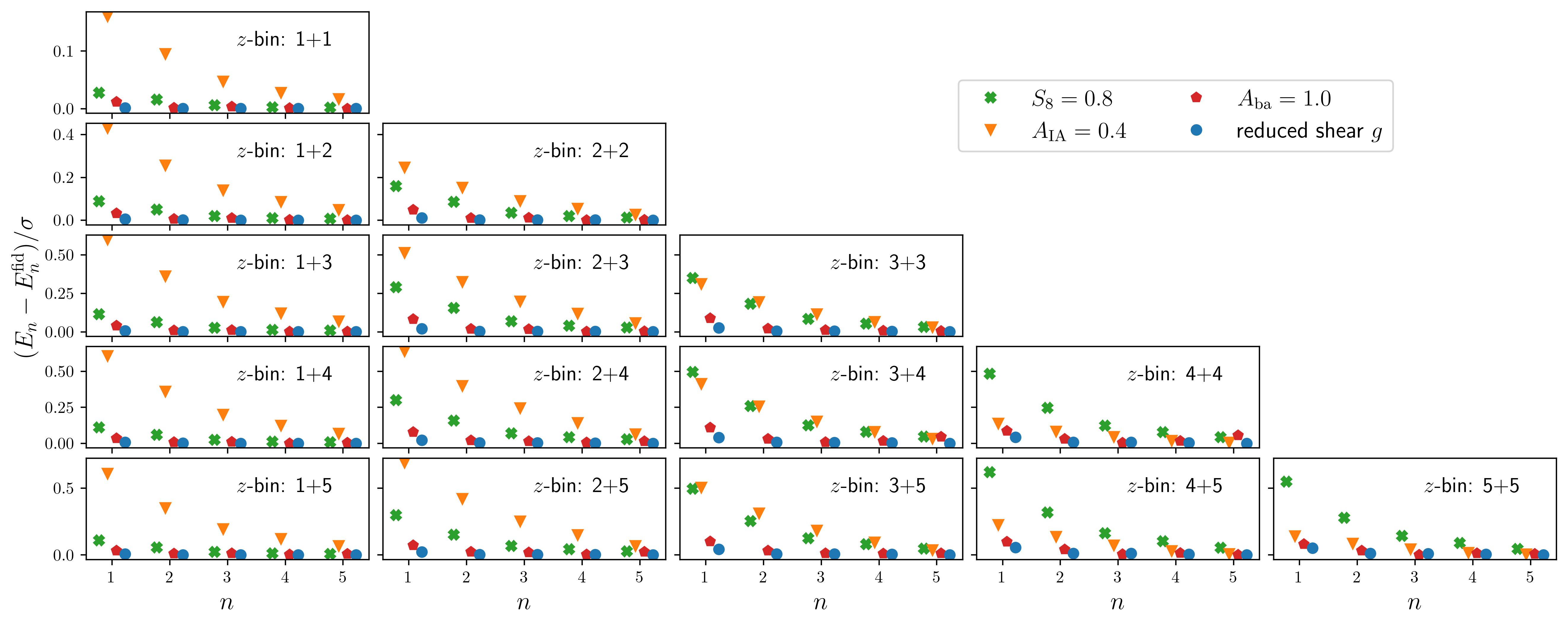
Figure 12: Illustration of several effects that change the $E_{n}$ model vector. The fiducial model $E_{n}^{\mathrm{fid}}$ is without reduced shear, $A_{\mathrm{IA}}=0$, $A_{\mathrm{ba}}=0$, $S_{8}=0.78$ and $\Omega_{\mathrm{m}}=0.25$. For the different points, one of the effects is changed. We scaled the model differences by the KiDS-1000 uncertainty, indicating the change’s relevance for this work.

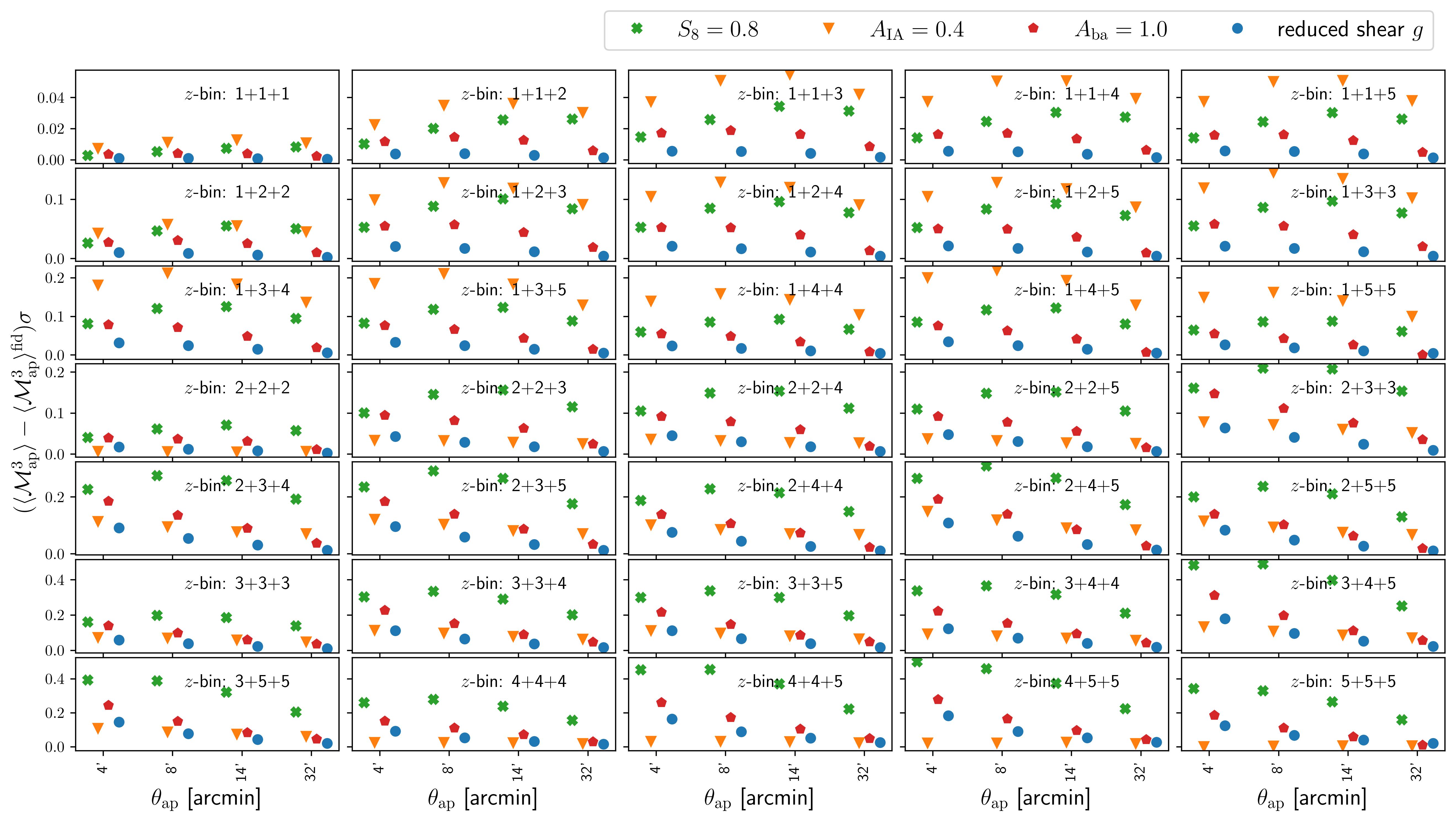
Figure 13: Same as Fig. 12 but for the ${\expectationvalue{\mathcal{M}_{\mathrm{ap}}^{3}}}$ model vector.

Appendix B Additional material

This appendix section is meant as a collection of figures to support the analysis in the main text. In Fig. 14, we show the full ${\expectationvalue{\mathcal{M}_{\mathrm{ap}}^{3}}}$ data vector for equal filter radii, from which we showed a subpart in Fig. 3. In Fig. 15, we show the ${\expectationvalue{\mathcal{M}_{\mathrm{ap}}^{3}}}$ data vector if non-equal filter radii are used and measured from the convergence T17 maps.

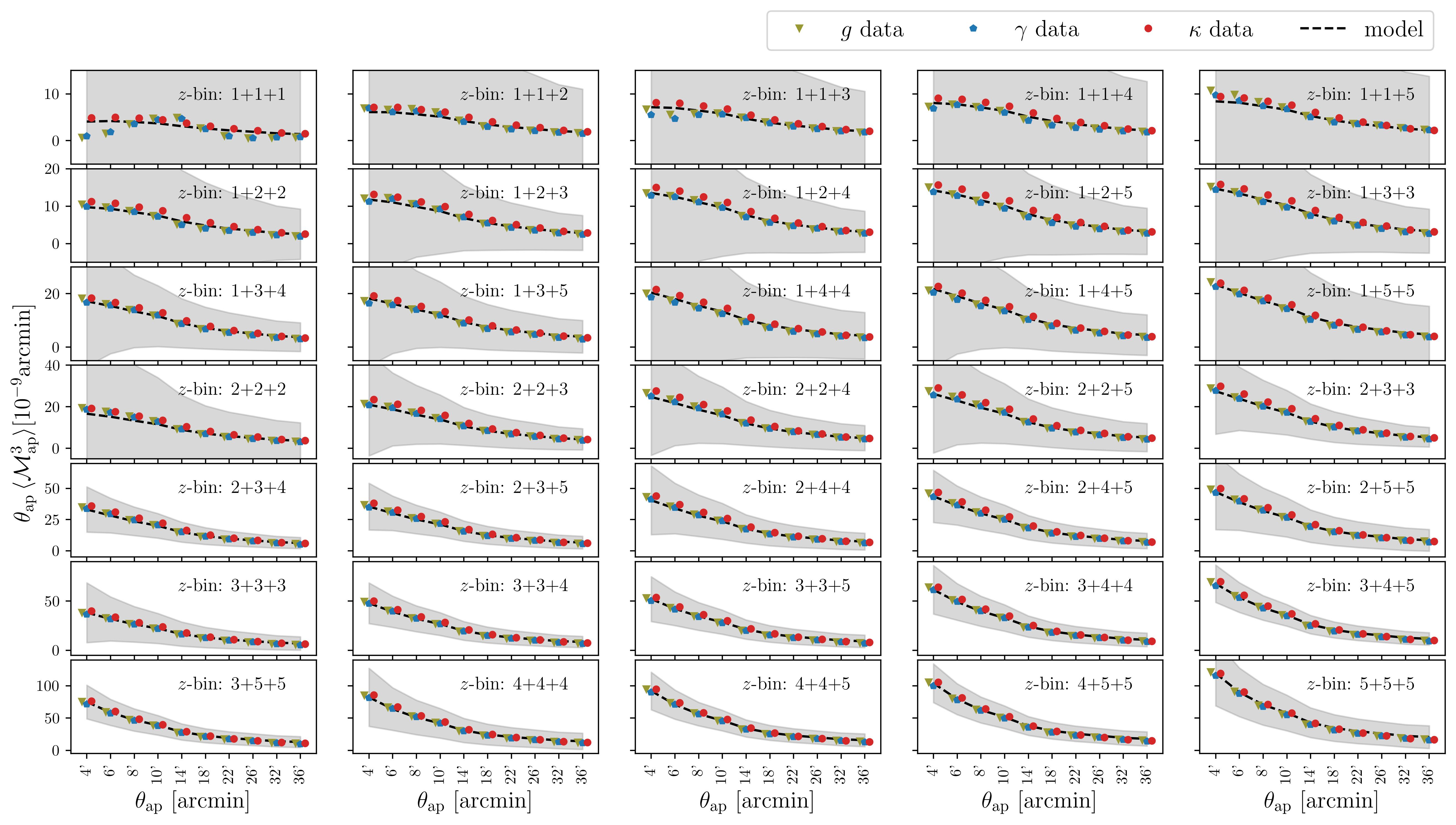
Figure 14: Same as Fig. 3, but here the measured data and model are the ${\expectationvalue{\mathcal{M}_{\mathrm{ap}}^{3}}}$ vector for equal-scale aperture filter radii $\theta_{\mathrm{ap}}\in\{$$,$$,$$,$$,$$,$$,$$,$$,$$,$$\}$ in the T17 mocks for $z$-bin combinations.

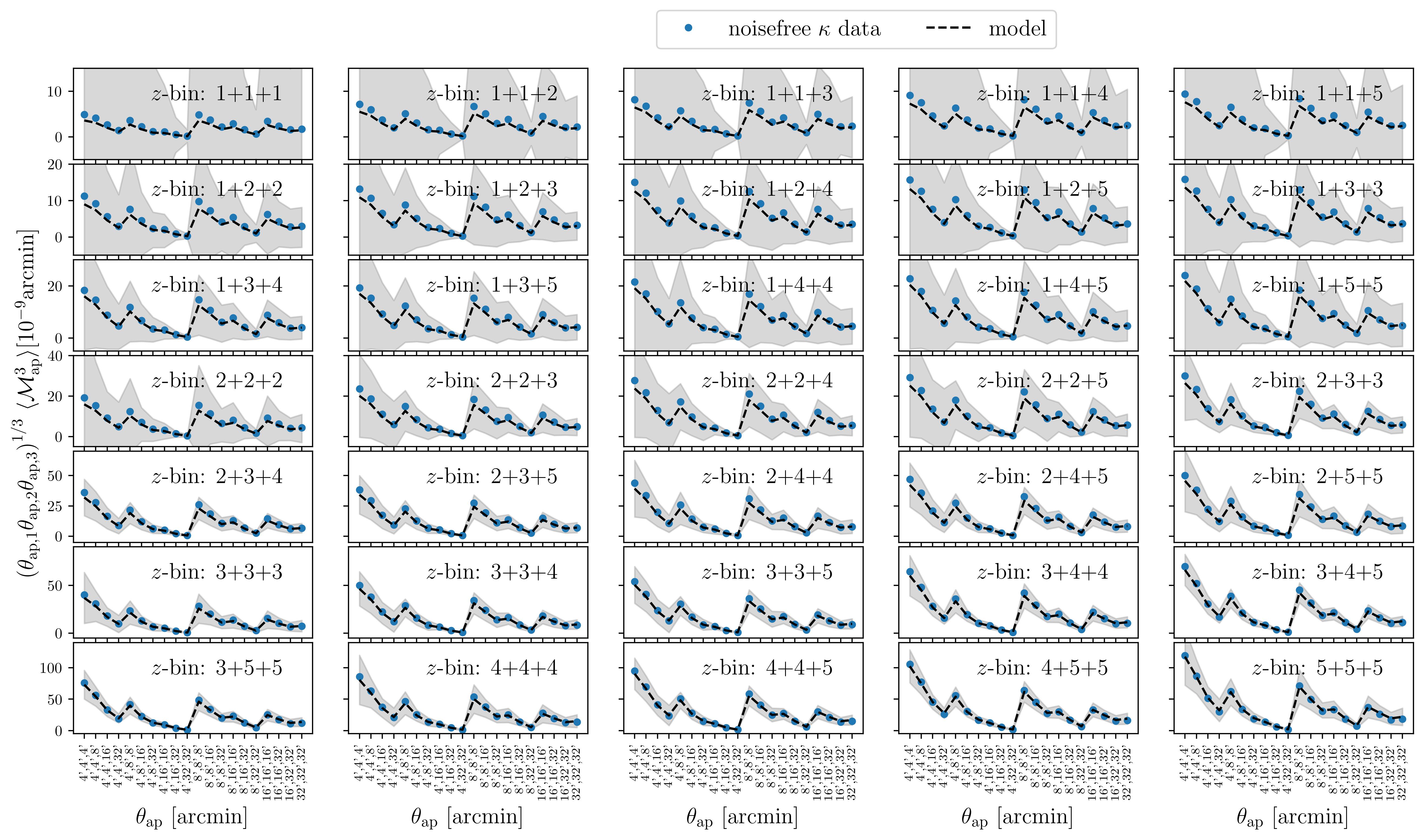
Figure 15: Measured data and model ${\expectationvalue{\mathcal{M}_{\mathrm{ap}}^{3}}}$ vector for all combinations of aperture filter radii $\theta_{\mathrm{ap}}\in\{$$,$$,$$,$$\}$. The data vector results from one full-sky convergence realisation without shape noise. The grey band shows the expected uncertainty of KiDS-1000 estimated with the convergence maps. The ${\expectationvalue{\mathcal{M}_{\mathrm{ap}}^{3}}}$ is scaled by the third root of the product of the corresponding filter radii.

References

- Abbott et al. (2022) Abbott, T. M. C., Aguena, M., Alarcon, A., et al. 2022, Phys. Rev. D, 105, 023520
- Asgari et al. (2019) Asgari, M., Heymans, C., Hildebrandt, H., et al. 2019, A&A, 624, A134
- Asgari et al. (2021) Asgari, M., Lin, C.-A., Joachimi, B., et al. 2021, A&A, 645, A104
- Asgari et al. (2020) Asgari, M., Tröster, T., Heymans, C., et al. 2020, A&A, 634, A127
- Bartelmann (2010) Bartelmann, M. 2010, Classical and Quantum Gravity, 27, 233001
- Bartelmann & Schneider (2001) Bartelmann, M. & Schneider, P. 2001, Phys. Rep, 340, 291
- Beck et al. (2016) Beck, A. M., Murante, G., Arth, A., et al. 2016, MNRAS, 455, 2110
- Bergé et al. (2010) Bergé, J., Amara, A., & Réfrégier, A. 2010, ApJ, 712, 992
- Bernardeau et al. (1997) Bernardeau, F., van Waerbeke, L., & Mellier, Y. 1997, A&A, 322, 1
- Bridle & King (2007) Bridle, S. & King, L. 2007, New Journal of Physics, 9, 444
- Brown et al. (2002) Brown, M. L., Taylor, A. N., Hambly, N. C., & Dye, S. 2002, MNRAS, 333, 501
- Burger et al. (2023) Burger, P. A., Friedrich, O., Harnois-Déraps, J., et al. 2023, A&A, 669, A69
- Castro et al. (2018) Castro, T., Quartin, M., Giocoli, C., Borgani, S., & Dolag, K. 2018, MNRAS, 478, 1305
- Chisari et al. (2015) Chisari, N., Codis, S., Laigle, C., et al. 2015, MNRAS, 454, 2736
- Crittenden et al. (2002) Crittenden, R. G., Natarajan, P., Pen, U.-L., & Theuns, T. 2002, ApJ, 568, 20
- Dalal et al. (2023) Dalal, R., Li, X., Nicola, A., et al. 2023, arXiv:2304.00701
- de Jong et al. (2015) de Jong, J. T. A., Verdoes Kleijn, G. A., Boxhoorn, D. R., et al. 2015, A&A, 582, A62
- de Jong et al. (2017) de Jong, J. T. A., Verdoes Kleijn, G. A., Erben, T., et al. 2017, A&A, 604, A134
- DES KiDS collaboration et al. (2023) DES KiDS collaboration, :, Abbott, T. M. C., et al. 2023, arXiv:2305.17173
- Di Valentino et al. (2021) Di Valentino, E., Anchordoqui, L. A., Akarsu, Ö., et al. 2021, Astroparticle Physics, 131, 102604
- Edge et al. (2013) Edge, A., Sutherland, W., Kuijken, K., et al. 2013, The Messenger, 154, 32
- Falco et al. (1985) Falco, E. E., Gorenstein, M. V., & Shapiro, I. I. 1985, ApJ, 289, L1
- Fenech Conti et al. (2017) Fenech Conti, I., Herbonnet, R., Hoekstra, H., et al. 2017, MNRAS, 467, 1627
- Fornberg (1988) Fornberg, B. 1988, Math. Comp., 184, 699–706
- Fu et al. (2014) Fu, L., Kilbinger, M., Erben, T., et al. 2014, MNRAS, 441, 2725
- Gatti et al. (2022) Gatti, M., Jain, B., Chang, C., et al. 2022, Phys. Rev. D, 106, 083509
- Gatti et al. (2023) Gatti, M., Jeffrey, N., Whiteway, L., et al. 2023, arXiv:2307.13860
- Giblin et al. (2021) Giblin, B., Heymans, C., Asgari, M., et al. 2021, A&A, 645, A105
- Górski et al. (2005) Górski, K. M., Hivon, E., Banday, A. J., et al. 2005, ApJ, 622, 759
- Gruen et al. (2018) Gruen, D., Friedrich, O., Krause, E., et al. 2018, Phys. Rev. D, 98, 023507
- Halder & Barreira (2022) Halder, A. & Barreira, A. 2022, MNRAS, 515, 4639
- Halder et al. (2021) Halder, A., Friedrich, O., Seitz, S., & Varga, T. N. 2021, MNRAS, 506, 2780
- Harnois-Déraps et al. (2018) Harnois-Déraps, J., Amon, A., Choi, A., et al. 2018, MNRAS, 481, 1337
- Harnois-Déraps et al. (2019) Harnois-Déraps, J., Giblin, B., & Joachimi, B. 2019, A&A, 631, A160
- Harnois-Déraps et al. (2021) Harnois-Déraps, J., Martinet, N., Castro, T., et al. 2021, MNRAS, 506, 1623
- Harnois-Déraps et al. (2022) Harnois-Déraps, J., Martinet, N., & Reischke, R. 2022, MNRAS, 509, 3868
- Harris et al. (2020) Harris, C. R., Millman, K. J., van der Walt, S. J., et al. 2020, Nature, 585, 357
- Heydenreich et al. (2021) Heydenreich, S., Brück, B., & Harnois-Déraps, J. 2021, A&A, 648, A74
- Heydenreich et al. (2023) Heydenreich, S., Linke, L., Burger, P., & Schneider, P. 2023, A&A, 672, A44
- Heymans et al. (2021) Heymans, C., Tröster, T., Asgari, M., et al. 2021, A&A, 646, A140
- Hikage et al. (2019) Hikage, C., Oguri, M., Hamana, T., et al. 2019, PASJ, 71, 43
- Hildebrandt et al. (2020) Hildebrandt, H., Köhlinger, F., van den Busch, J. L., et al. 2020, A&A, 633, A69
- Hildebrandt et al. (2021) Hildebrandt, H., van den Busch, J. L., Wright, A. H., et al. 2021, A&A, 647, A124
- Hildebrandt et al. (2017) Hildebrandt, H., Viola, M., Heymans, C., et al. 2017, MNRAS, 465, 1454
- Hinton (2016) Hinton, S. R. 2016, The Journal of Open Source Software, 1, 00045
- Hirschmann et al. (2014) Hirschmann, M., Dolag, K., Saro, A., et al. 2014, MNRAS, 442, 2304
- Hoekstra & Jain (2008) Hoekstra, H. & Jain, B. 2008, Annual Review of Nuclear and Particle Science, 58, 99
- Hunter (2007) Hunter, J. D. 2007, Computing in Science & Engineering, 9, 90
- Ivezic et al. (2008) Ivezic, Z., Axelrod, T., Brandt, W. N., et al. 2008, Serbian Astronomical Journal, 176, 1
- Jarvis et al. (2004) Jarvis, M., Bernstein, G., & Jain, B. 2004, MNRAS, 352, 338
- Joachimi et al. (2015) Joachimi, B., Cacciato, M., Kitching, T. D., et al. 2015, Space Sci. Rev., 193, 1
- Joachimi et al. (2021) Joachimi, B., Lin, C. A., Asgari, M., et al. 2021, A&A, 646, A129
- Jones et al. (2001) Jones, E., Oliphant, T., Peterson, P., et al. 2001, SciPy: Open source scientific tools for Python
- Joudaki et al. (2020) Joudaki, S., Hildebrandt, H., Traykova, D., et al. 2020, A&A, 638, L1
- Kaiser & Jaffe (1997) Kaiser, N. & Jaffe, A. 1997, ApJ, 484, 545
- Kannawadi et al. (2019) Kannawadi, A., Hoekstra, H., Miller, L., et al. 2019, A&A, 624, A92
- Kilbinger (2015) Kilbinger, M. 2015, Reports on Progress in Physics, 78, 086901
- Kilbinger et al. (2017) Kilbinger, M., Heymans, C., Asgari, M., et al. 2017, MNRAS, 472, 2126
- Kilbinger & Schneider (2005) Kilbinger, M. & Schneider, P. 2005, A&A, 442, 69
- Kuijken et al. (2019) Kuijken, K., Heymans, C., Dvornik, A., et al. 2019, A&A, 625
- Kuijken et al. (2015) Kuijken, K., Heymans, C., Hildebrandt, H., et al. 2015, MNRAS, 454, 3500
- Laureijs et al. (2011) Laureijs, R., Amiaux, J., Arduini, S., et al. 2011, arXiv:1110.3193
- Li et al. (2023) Li, S.-S., Hoekstra, H., Kuijken, K., et al. 2023, arXiv:2306.11124
- Limber (1954) Limber, D. N. 1954, ApJ, 119, 655
- Linke et al. (2023) Linke, L., Heydenreich, S., Burger, P. A., & Schneider, P. 2023, A&A, 672, A185
- LoVerde & Afshordi (2008) LoVerde, M. & Afshordi, N. 2008, Phys. Rev. D, 78, 123506
- Martinet et al. (2018) Martinet, N., Schneider, P., Hildebrandt, H., et al. 2018, MNRAS, 474, 712
- Mead et al. (2021) Mead, A. J., Brieden, S., Tröster, T., & Heymans, C. 2021, MNRAS, 502, 1401
- Miller et al. (2013) Miller, L., Heymans, C., Kitching, T. D., et al. 2013, MNRAS, 429, 2858
- Munshi et al. (2008) Munshi, D., Valageas, P., van Waerbeke, L., & Heavens, A. 2008, Phys. Rep, 462, 67
- Percival et al. (2022) Percival, W. J., Friedrich, O., Sellentin, E., & Heavens, A. 2022, MNRAS, 510, 3207
- Pires et al. (2012) Pires, S., Leonard, A., & Starck, J.-L. 2012, MNRAS, 423, 983
- Planck Collaboration et al. (2020) Planck Collaboration, Aghanim, N., Akrami, Y., et al. 2020, A&A, 641, A6
- Porth et al. (2023) Porth, L., Heydenreich, S., Burger, P., Linke, L., & Schneider, P. 2023, arXiv:2309.08601
- Pyne & Joachimi (2021) Pyne, S. & Joachimi, B. 2021, MNRAS, 503, 2300
- Ragagnin et al. (2017) Ragagnin, A., Dolag, K., Biffi, V., et al. 2017, Astronomy and Computing, 20, 52
- Sánchez et al. (2017) Sánchez, A. G., Scoccimarro, R., Crocce, M., et al. 2017, MNRAS, 464, 1640
- Schneider (1996) Schneider, P. 1996, MNRAS, 283, 837
- Schneider et al. (2010) Schneider, P., Eifler, T., & Krause, E. 2010, A&A, 520, A116
- Schneider et al. (2005) Schneider, P., Kilbinger, M., & Lombardi, M. 2005, A&A, 431, 9
- Schneider & Lombardi (2003) Schneider, P. & Lombardi, M. 2003, A&A, 397, 809
- Schneider & Seitz (1995) Schneider, P. & Seitz, C. 1995, A&A, 294, 411
- Schneider et al. (1998) Schneider, P., van Waerbeke, L., Jain, B., & Kruse, G. 1998, MNRAS, 296, 873
- Schneider et al. (2002) Schneider, P., van Waerbeke, L., & Mellier, Y. 2002, A&A, 389, 729
- Secco et al. (2022) Secco, L. F., Jarvis, M., Jain, B., et al. 2022, Phys. Rev. D, 105, 103537
- Seitz & Schneider (1997) Seitz, C. & Schneider, P. 1997, A&A, 318, 687
- Springel (2005) Springel, V. 2005, MNRAS, 364, 1105
- Spurio Mancini et al. (2022) Spurio Mancini, A., Piras, D., Alsing, J., Joachimi, B., & Hobson, M. P. 2022, MNRAS, 511, 1771
- Takahashi et al. (2017) Takahashi, R., Hamana, T., Shirasaki, M., et al. 2017, ApJ, 850, 24
- Takahashi et al. (2020) Takahashi, R., Nishimichi, T., Namikawa, T., et al. 2020, ApJ, 895, 113
- Tegmark et al. (1997) Tegmark, M., Taylor, A. N., & Heavens, A. F. 1997, ApJ, 480, 22
- Troxel & Ishak (2012) Troxel, M. A. & Ishak, M. 2012, MNRAS, 419, 1804
- Troxel et al. (2018) Troxel, M. A., MacCrann, N., Zuntz, J., et al. 2018, Phys. Rev. D, 98, 043528
- van Daalen et al. (2011) van Daalen, M. P., Schaye, J., Booth, C. M., & Dalla Vecchia, C. 2011, MNRAS, 415, 3649
- van den Busch et al. (2022) van den Busch, J. L., Wright, A. H., Hildebrandt, H., et al. 2022, A&A, 664, A170
- Wright et al. (2020) Wright, A. H., Hildebrandt, H., van den Busch, J. L., et al. 2020, A&A, 640, L14
- Zonca et al. (2019) Zonca, A., Singer, L., Lenz, D., et al. 2019, Journal of Open Source Software, 4, 1298
- Zuntz et al. (2015a) Zuntz, J., Paterno, M., Jennings, E., et al. 2015a, Astronomy and Computing, 12, 45
- Zuntz et al. (2015b) Zuntz, J., Paterno, M., Jennings, E., et al. 2015b, Astronomy and Computing, 12, 45