11institutetext: 1University of Bonn, Argelander-Institut für Astronomie, Auf dem Hügel 71, 53121 Bonn, Germany
2 Department of Astronomy and Astrophysics, University of California, Santa Cruz, 1156 High Street, Santa Cruz, CA 95064 USA
3 Universität Innsbruck, Institut für Astro- und Teilchenphysik, Technikerstr. 25/8, 6020 Innsbruck, Austria

A roadmap to cosmological parameter analysis with third-order shear statistics III: Efficient estimation of third-order shear correlation functions and an application to the KiDS-1000 data

Lucas Porth    1 Sven Heydenreich E-mail: lporth@astro.uni-bonn.de    1,2 Pierre Burger    1 Laila Linke    1,3 Peter Schneider1

Context. Third-order lensing statistics contain a wealth of cosmological information that is not captured by second-order statistics. However, the computational effort for estimating such statistics on forthcoming stage IV surveys is prohibitively expensive.
Aims. We derive and validate an efficient estimation procedure for the three-point correlation function (3PCF) of polar fields such as weak lensing shear. We then use our approach to measure the shear 3PCF and the third-order aperture mass statistics on the KiDS-1000 survey.
Methods. We construct an efficient estimator for third-order shear statistics which builds on the multipole decomposition of the 3PCF. We then validate our estimator on mock ellipticity catalogs obtained from N𝑁N-body simulations. Finally, we apply our estimator to the KiDS-1000 data and present a measurement of the third-order aperture statistics in a tomographic setup.
Results. Our estimator provides a speedup of a factor of 100similar-toabsent100\sim\!100 - 100010001000 compared to the state-of-the-art estimation procedures. It is also able to provide accurate measurements for squeezed and folded triangle configurations without additional computational effort. We report a significant detection of the tomographic third-order aperture mass statistics in the KiDS-1000 data (S/N=6.69)SN6.69(\mathrm{S/N}=6.69).
Conclusions. Our estimator will make it computationally feasible to measure third-order shear statistics in forthcoming stage IV surveys. Furthermore, it can be used to construct empirical covariance matrices for such statistics.

Key Words.:
gravitational lensing: weak – methods: numerical – large-scale structure of Universe

1 Introduction

The most widely used set of statistics for extracting cosmological information from galaxy or weak gravitational lensing surveys is related to N𝑁N-point correlation functions (N𝑁NPCFs). Estimating those quantities from the position or shapes of a set of observed tracers, one reveals parts of the statistical properties of the underlying cosmic large-scale structure. In particular, for weak gravitational lensing surveys the analysis of shear 222PCFs and its harmonic analog, the power spectrum, have made it possible to put tight constraints on the matter clustering parameter S8σ8Ωm/0.3subscript𝑆8subscript𝜎8subscriptΩm0.3S_{8}\equiv\sigma_{8}\sqrt{\Omega_{\mathrm{m}}/0.3}, where σ8subscript𝜎8\sigma_{8} is the normalization of the matter power spectrum and ΩmsubscriptΩm\Omega_{\mathrm{m}} is the matter density parameter (Heymans et al. 2013; Hildebrandt et al. 2017; Troxel et al. 2018; Hikage et al. 2019; Hamana et al. 2020; Asgari et al. 2021; Amon et al. 2022; Secco et al. 2022; Dalal et al. 2023; Li et al. 2023).

While most of the theoretical and observational work has been done at the second-order level, it is well known that through this choice one is sensitive only to the Gaussian information of the density field. To extract additional information including contributions from non-linear structure formation, one needs to resort to other higher-order statistics, some of which are related to higher-order moments (Jain & Seljak 1997; Schneider et al. 1998; Vicinanza et al. 2018; Gatti et al. 2020), peaks (Kruse & Schneider 1999; Hamana et al. 2004; Harnois-Déraps et al. 2021), the one-point probability distribution function (Patton et al. 2017; Barthelemy et al. 2020; Boyle et al. 2021; Giblin et al. 2023), or the topological properties (Kratochvil et al. 2012; Parroni et al. 2020; Heydenreich et al. 2022) of the density field. Besides the gain in cosmological information, it has been shown that when performing a joint analysis together with second-order statistics, higher-order statistics can also break degeneracies between parameters of cosmological, astrophysical or systematic origin and therefore have the potential to yield much tighter cosmological constraints (Kilbinger & Schneider 2005; Takada & Jain 2003; Semboloni et al. 2008; Pyne & Joachimi 2021).

Higher-order statistics from the correlation function hierarchy consist of the (N>2)𝑁2(N>2)-point correlation functions, from which the three-point correlation function (3PCF) is the most prominent example (Schneider & Lombardi 2003; Zaldarriaga & Scoccimarro 2003). Besides the challenges to accurately model the cosmological and observational effects on the shape of the 3PCF (Takada & Jain 2003; Heydenreich et al. 2023), it is also computationally much more expensive to estimate them, compared to the 2PCF. A naive estimator would require putting all triplets of tracers into a predefined set of bins describing the triplets’ configuration. The resulting computational complexity for a survey of Ngalsubscript𝑁galN_{\mathrm{gal}} tracers is 𝒪(Ngal3)𝒪superscriptsubscript𝑁gal3\mathcal{O}(N_{\mathrm{gal}}^{3}), rendering this brute-force approach computationally prohibitive. To facilitate an estimation of the 3PCF of scalar (spin-0) and polar (spin-2) observables for current surveys, k𝑘kd-tree based methods have been developed (Jarvis et al. 2004; Zhang & Pen 2005; Kilbinger et al. 2014) and applied to a wide range of data sets (Bernardeau et al. 2002; Semboloni et al. 2011; Fu et al. 2014; Secco et al. 2022). Even though the computational speedup compared to the brute-force estimator is remarkable, it is most likely still too time-consuming to apply it to stage IV cosmic shear surveys like Euclid (Laureijs et al. 2011) or the Vera Rubin Observatory Legacy Survey of Space and Time (Ivezić et al. 2019). A different class of estimators has been tailored towards the multipole components of the N𝑁NPCFs of scalar fields (Chen & Szapudi 2005; Slepian & Eisenstein 2015; Philcox et al. 2022). As the multipoles can be estimated in quadratic time complexity for a discrete galaxy catalog, or with an Npixlog(Npix)subscript𝑁pixsubscript𝑁pixN_{\mathrm{pix}}\log(N_{\mathrm{pix}}) scaling for data distributed on a grid of Npixsubscript𝑁pixN_{\mathrm{pix}} pixels, this estimation strategy makes it feasible to efficiently and accurately measure higher-order correlation functions on large data sets. For example, the first measurement of the 4PCF of the scalar galaxy position field was presented in Hou et al. (2022) and Philcox (2022).

In this work, we extend the multipole decomposition of the scalar 3PCF to the natural components of the 3PCF associated with spin-2 tracer fields, such as weak lensing shear. Additionally, we construct an efficient estimator that adaptively switches between a discrete and grid-based prescription for triangle sides of different lengths. With those modifications, we can measure the full 3PCF for any triangle configuration on a stage-III survey in a few CPU hours without significantly sacrificing accuracy compared to the brute-force estimator.

This work belongs to a series of papers that aim for a cosmological parameter analysis using third-order shear statistics. Heydenreich et al. (2023) introduces an analytical model for the third-order aperture statistics based on the Bihalofit formula (Takahashi et al. 2020) for the matter bispectrum. In Linke et al. (2023), an analytical covariance matrix for the third-order aperture statistics is derived in the presence of a finite survey extent. Burger et al. (2023) extends the analytical model to a tomographic setting, includes methods to account for the impact of intrinsic alignments and baryonic feedback, and presents a cosmological analysis using a joint data vector of the COSEBIs and the third-order aperture mass statistics measured in the KiDS-1000 data.

This paper is structured as follows. In Sect. 2, we introduce the shear 3PCF and their natural components ΓμsubscriptΓ𝜇\Gamma_{\mu}. In Sect. 3, we derive our estimator for the ΓμsubscriptΓ𝜇\Gamma_{\mu} and discuss some approximations. In Sect. 4, we validate our estimator on a large suite of N-body simulations, the SLICS ensemble, and compare it with measurements obtained with TREECORR (Jarvis et al. 2004). In Sect. 5 we introduce the third-order aperture measures, show how they can be obtained from our shear 3PCF estimator and validate our implementation. In Sect. 6, we apply our estimator to the fourth data release of the Kilo Degree Survey (Kuijken et al. 2019, hereafter KiDS-1000). After obtaining an empirical estimate of the expected correlation matrix for the KiDS-1000 data from a large suite of mock catalogs we present our measurement of the third-order aperture statistics in the KiDS-1000 data. We conclude in Sect. 7.

2 Third-order measures of cosmic shear

This section aims to introduce the main concepts related to weak gravitational lensing with an emphasis on the third-order shear correlation functions; for extensive reviews of the weak gravitational lensing see Bartelmann & Schneider (2001); Kilbinger (2015); Dodelson (2017); Mandelbaum (2018). In order to keep the notation concise, we do not consider tomographic setups in this and the following section but collect the corresponding expressions in Sect. 3.5. Furthermore, we do not consider higher-order effects like reduced shear, source redshift clustering, or astrophysical effects, such as intrinsic alignments.

2.1 Basic notions

The two fundamental quantities in weak gravitational lensing are the convergence κ𝜅\kappa and the shear γ𝛾\gamma, which describe the isotropic stretching and distortion experienced by a light bundle propagating through spacetime. The convergence κ𝜅\kappa can be written as a weighted projection of the density contrast δ𝛿\delta along the line of sight

κ(𝜽)=0χmaxdχW(χ)δ[fK(χ)𝜽;χ],𝜅𝜽superscriptsubscript0subscript𝜒maxsuperscript𝜒𝑊superscript𝜒𝛿subscript𝑓𝐾superscript𝜒𝜽superscript𝜒\displaystyle\kappa(\boldsymbol{\theta})=\int_{0}^{\chi_{\mathrm{max}}}\differential\chi^{\prime}W(\chi^{\prime})\ \delta\left[f_{K}(\chi^{\prime})\boldsymbol{\theta};\chi^{\prime}\right]\ , (1)

where the associated projection kernel W𝑊W is defined as

W(χ)3ΩmH022c2fK(χ)a(χ)z(χ)dzn(z)fK[χ(z)χ]fK[χ(z)]𝑊𝜒3subscriptΩmsuperscriptsubscript𝐻022superscript𝑐2subscript𝑓𝐾𝜒𝑎𝜒superscriptsubscript𝑧𝜒superscript𝑧𝑛superscript𝑧subscript𝑓𝐾delimited-[]𝜒superscript𝑧𝜒subscript𝑓𝐾delimited-[]𝜒superscript𝑧\displaystyle W(\chi)\equiv\frac{3\Omega_{\mathrm{m}}H_{0}^{2}}{2c^{2}}\frac{f_{K}(\chi)}{a(\chi)}\int_{z(\chi)}^{\infty}\differential z^{\prime}n(z^{\prime})\frac{f_{K}[\chi(z^{\prime})-\chi]}{f_{K}[\chi(z^{\prime})]} (2)

and fK[χ(z)]subscript𝑓𝐾delimited-[]𝜒𝑧f_{K}[\chi(z)] denotes the comoving angular diameter distance of the comoving radial distance χ𝜒\chi at redshift z𝑧z and we introduced the dimensionless matter density parameter ΩmsubscriptΩm\Omega_{\mathrm{m}} and the Hubble constant H0subscript𝐻0H_{0}, as well as the scale factor a𝑎a and the source redshift distribution n(z)𝑛𝑧n(z). For the remainder of this work, we assume a flat universe for which fK(χ)=χsubscript𝑓𝐾𝜒𝜒f_{K}(\chi)=\chi.

The components of the complex shear field γ𝛾\gamma can be characterised with respect to a Cartesian coordinate frame, γcγ1+iγ2subscript𝛾csubscript𝛾1isubscript𝛾2\gamma_{\mathrm{c}}\equiv\gamma_{1}+\mathrm{i}\gamma_{2}. To evaluate the shear at position 𝜽𝜽\boldsymbol{\theta} in a reference frame, that is rotated by an angle ζ𝜁\zeta with respect to the Cartesian basis one has

γ(𝜽;ζ)[γt(𝜽;ζ)+iγ×(𝜽;ζ)]γc(𝜽)e2iζ,𝛾𝜽𝜁delimited-[]subscript𝛾t𝜽𝜁isubscript𝛾𝜽𝜁subscript𝛾c𝜽superscripte2i𝜁\displaystyle\gamma(\boldsymbol{\theta};\zeta)\equiv-\left[\gamma_{\mathrm{t}}(\boldsymbol{\theta};\zeta)+\mathrm{i}\gamma_{\times}(\boldsymbol{\theta};\zeta)\right]\equiv-\gamma_{\mathrm{c}}(\boldsymbol{\theta})\ \mathrm{e}^{-2\mathrm{i}\zeta}\ , (3)

where we introduced the tangential (γt)subscript𝛾t(\gamma_{\mathrm{t}}) and cross-components (γ×)subscript𝛾(\gamma_{\times}) of the shear with respect to the projection direction ζ𝜁\zeta.

2.2 The shear 3PCF and its natural components

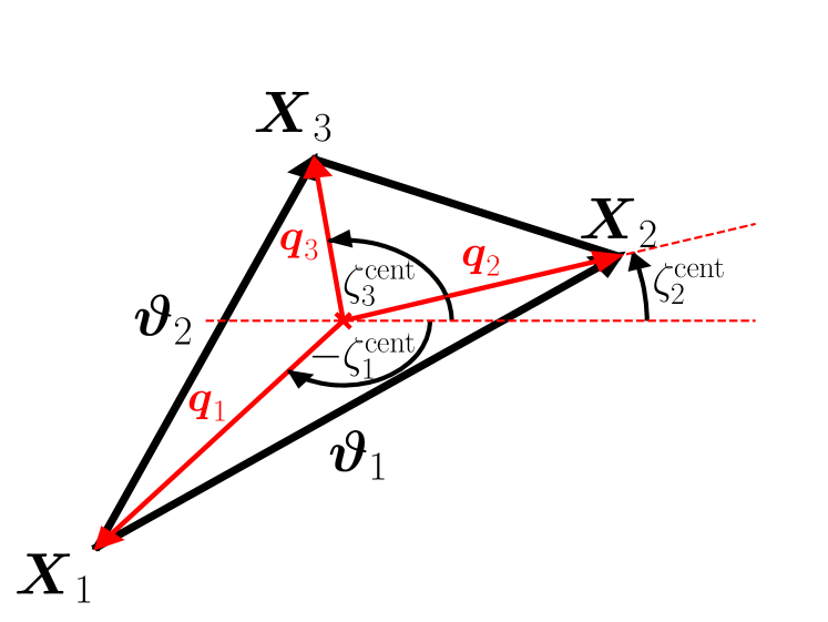
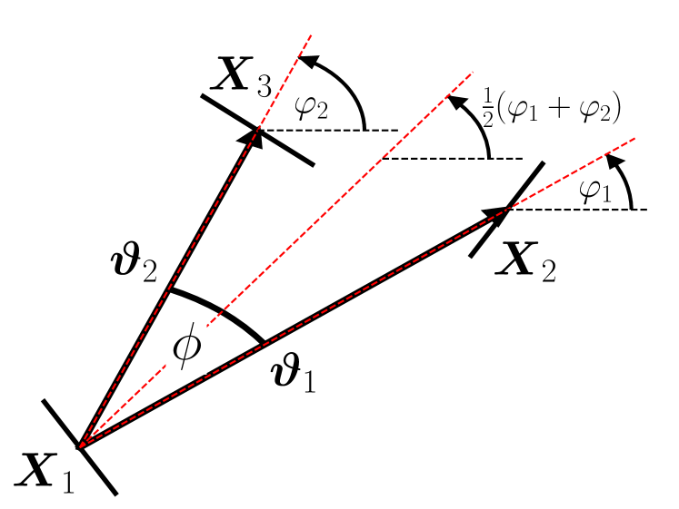
Due to the polar nature of the shear, there are 888 different real-valued components for its three-point correlator. Schneider & Lombardi (2003) regroup those components into four complex-valued natural components ΓμsubscriptΓ𝜇\Gamma_{\mu}, that do not mix and only transform by some phase factor under rotations of the corresponding triangle. Parameterizing a triangle as depicted in Fig. 1 and choosing some arbitrary projection 𝓟𝓟\boldsymbol{\mathcal{P}} in which the individual shear components are rotated by angles ζisubscript𝜁𝑖\zeta_{i}, we define the natural components of the shear 3PCF as111We note that our definition of the Γμ𝓟superscriptsubscriptΓ𝜇𝓟\Gamma_{\mu}^{\boldsymbol{\mathcal{P}}} is different from the one found in Schneider & Lombardi (2003), but instead matches the configuration of the third-order correlators introduced in Jarvis et al. (2004) and the TREECORR implementation.

Γ0𝓟(ϑ1,ϑ2,ϕ)superscriptsubscriptΓ0𝓟subscriptitalic-ϑ1subscriptitalic-ϑ2italic-ϕ\displaystyle\Gamma_{0}^{\boldsymbol{\mathcal{P}}}(\vartheta_{1},\vartheta_{2},\phi) =γ(𝐗𝟏;ζ1)γ(𝐗𝟐;ζ2)γ(𝐗𝟑;ζ3),absentdelimited-⟨⟩𝛾subscript𝐗1subscript𝜁1𝛾subscript𝐗2subscript𝜁2𝛾subscript𝐗3subscript𝜁3\displaystyle=\left\langle\ \gamma\left(\mathbf{X_{1}};\zeta_{1}\right)\ \gamma\left(\mathbf{X_{2}};\zeta_{2}\right)\ \gamma\left(\mathbf{X_{3}};\zeta_{3}\right)\ \right\rangle\ , (4)
Γ1𝓟(ϑ1,ϑ2,ϕ)superscriptsubscriptΓ1𝓟subscriptitalic-ϑ1subscriptitalic-ϑ2italic-ϕ\displaystyle\Gamma_{1}^{\boldsymbol{\mathcal{P}}}(\vartheta_{1},\vartheta_{2},\phi) =γ(𝐗𝟏;ζ1)γ(𝐗𝟐;ζ2)γ(𝐗𝟑;ζ3),absentdelimited-⟨⟩superscript𝛾subscript𝐗1subscript𝜁1𝛾subscript𝐗2subscript𝜁2𝛾subscript𝐗3subscript𝜁3\displaystyle=\left\langle\ \gamma^{*}\left(\mathbf{X_{1}};\zeta_{1}\right)\ \gamma\left(\mathbf{X_{2}};\zeta_{2}\right)\ \gamma\left(\mathbf{X_{3}};\zeta_{3}\right)\ \right\rangle\ , (5)
Γ2𝓟(ϑ1,ϑ2,ϕ)superscriptsubscriptΓ2𝓟subscriptitalic-ϑ1subscriptitalic-ϑ2italic-ϕ\displaystyle\Gamma_{2}^{\boldsymbol{\mathcal{P}}}(\vartheta_{1},\vartheta_{2},\phi) =γ(𝐗𝟏;ζ1)γ(𝐗𝟐;ζ2)γ(𝐗𝟑;ζ3),absentdelimited-⟨⟩𝛾subscript𝐗1subscript𝜁1superscript𝛾subscript𝐗2subscript𝜁2𝛾subscript𝐗3subscript𝜁3\displaystyle=\left\langle\ \gamma\left(\mathbf{X_{1}};\zeta_{1}\right)\ \gamma^{*}\left(\mathbf{X_{2}};\zeta_{2}\right)\ \gamma\left(\mathbf{X_{3}};\zeta_{3}\right)\ \right\rangle\ , (6)
Γ3𝓟(ϑ1,ϑ2,ϕ)superscriptsubscriptΓ3𝓟subscriptitalic-ϑ1subscriptitalic-ϑ2italic-ϕ\displaystyle\Gamma_{3}^{\boldsymbol{\mathcal{P}}}(\vartheta_{1},\vartheta_{2},\phi) =γ(𝐗𝟏;ζ1)γ(𝐗𝟐;ζ2)γ(𝐗𝟑;ζ3),absentdelimited-⟨⟩𝛾subscript𝐗1subscript𝜁1𝛾subscript𝐗2subscript𝜁2superscript𝛾subscript𝐗3subscript𝜁3\displaystyle=\left\langle\ \gamma\left(\mathbf{X_{1}};\zeta_{1}\right)\ \gamma\left(\mathbf{X_{2}};\zeta_{2}\right)\ \gamma^{*}\left(\mathbf{X_{3}};\zeta_{3}\right)\ \right\rangle\ , (7)

where ϑi|ϑi|subscriptitalic-ϑ𝑖subscriptbold-italic-ϑ𝑖\vartheta_{i}\equiv|\boldsymbol{\vartheta}_{i}| and we have assumed that the projection directions ζisubscript𝜁𝑖\zeta_{i} are defined in terms of the vertices of the triangle; this implies that the natural components are invariant under rotations of the triangle such that a parametrization in terms of three variables is sufficient. We note that any of the natural components can be written in terms of the elements

{γttt,γ×tt,γt×t,γtt×,γt××,γ×t×,γ××t,γ×××},subscript𝛾tttsubscript𝛾absentttsubscript𝛾ttsubscript𝛾ttsubscript𝛾tabsentsubscript𝛾absenttsubscript𝛾absenttsubscript𝛾absent\displaystyle\{\gamma_{\mathrm{t}\mathrm{t}\mathrm{t}},\gamma_{\times\mathrm{t}\mathrm{t}},\gamma_{\mathrm{t}\times\mathrm{t}},\gamma_{\mathrm{t}\mathrm{t}\times},\gamma_{\mathrm{t}\times\times},\gamma_{\times\mathrm{t}\times},\gamma_{\times\times\mathrm{t}},\gamma_{\times\times\times}\}\ , (8)

where we introduced shorthand notation like γtttγtγtγtsubscript𝛾tttdelimited-⟨⟩subscript𝛾tsubscript𝛾tsubscript𝛾t\gamma_{\mathrm{t}\mathrm{t}\mathrm{t}}\equiv\left\langle\gamma_{\mathrm{t}}\gamma_{\mathrm{t}}\gamma_{\mathrm{t}}\right\rangle for the various triple products of shears (Schneider & Lombardi 2003). Inverting the relations (4)–(7) one can relate the components in Eq. (8) to the natural components.

2.3 Choice of projections for the shear 3PCF

For this work, we employ two particular projections. The first of them, which we dub the ×\times-projection, is defined by the rotation angles

ζ1×=12(φ1+φ2),ζ2×=φ1,ζ3×=φ2\displaystyle\zeta_{1}^{\times}=\frac{1}{2}\left(\varphi_{1}+\varphi_{2}\right)\ \ \ ,\ \ \ \zeta_{2}^{\times}=\varphi_{1}\ \ \ ,\ \ \ \zeta_{3}^{\times}=\varphi_{2}\ \ (9)

and the corresponding projection axes are depicted in the upper panel of Fig. 1. As we will see later, this projection turns out to be useful for the estimator derived in Sect. 3. For the second projection shown in the lower panel of Fig. 1, we first define the centroid of the triangle as the intersection of its three medians and then project the shear at position 𝐗isubscript𝐗𝑖\mathbf{X}_{i} along the direction qisubscriptq𝑖\mathrm{\textbf{{q}}}_{i} of the median passing through 𝐗isubscript𝐗𝑖\mathbf{X}_{i}:

e2iζ1cent=q˘1q˘1,e2iζ2cent=q˘2q˘2,e2iζ3cent=q˘3q˘3,\displaystyle\mathrm{e}^{2\mathrm{i}\zeta_{1}^{\mathrm{cent}}}=\frac{\breve{\mathrm{\textbf{{q}}}}_{1}}{\breve{\mathrm{\textbf{{q}}}}_{1}^{*}}\ \ \ ,\ \ \ \mathrm{e}^{2\mathrm{i}\zeta_{2}^{\mathrm{cent}}}=\frac{\breve{\mathrm{\textbf{{q}}}}_{2}}{\breve{\mathrm{\textbf{{q}}}}_{2}^{*}}\ \ \ ,\ \ \ \mathrm{e}^{2\mathrm{i}{\zeta_{3}^{\mathrm{cent}}}}=\frac{\breve{\mathrm{\textbf{{q}}}}_{3}}{\breve{\mathrm{\textbf{{q}}}}_{3}^{*}}\ , (10)

where the qisubscriptq𝑖\mathrm{\textbf{{q}}}_{i} are given as

q1=ϑ1+ϑ23,q2=2ϑ1ϑ23,q3=2ϑ2ϑ13\displaystyle\mathrm{\textbf{{q}}}_{1}=-\frac{\boldsymbol{\vartheta}_{1}+\boldsymbol{\vartheta}_{2}}{3}\ \ \ ,\ \ \ \mathrm{\textbf{{q}}}_{2}=\frac{2\boldsymbol{\vartheta}_{1}-\boldsymbol{\vartheta}_{2}}{3}\ \ \ ,\ \ \ \mathrm{\textbf{{q}}}_{3}=\frac{2\boldsymbol{\vartheta}_{2}-\boldsymbol{\vartheta}_{1}}{3} (11)

and we defined q˘iqi,1+iqi,2subscript˘q𝑖subscript𝑞𝑖1isubscript𝑞𝑖2\breve{\mathrm{\textbf{{q}}}}_{i}\equiv q_{i,1}+\mathrm{i}q_{i,2}. The corresponding ΓμcentsuperscriptsubscriptΓ𝜇cent\Gamma_{\mu}^{\mathrm{cent}} are useful for connecting the shear 3PCF to the third-order aperture statistics and is being used by other estimators for the 3PCF such as TREECORR .

We can convert between the two projections using Eq. (3). For example, the zeroth natural component in the ×\times-projection can be written as

Γ0×(ϑ1,ϑ2,ϕ)subscriptsuperscriptΓ0subscriptitalic-ϑ1subscriptitalic-ϑ2italic-ϕ\displaystyle\Gamma^{\mathrm{\times}}_{0}(\vartheta_{1},\vartheta_{2},\phi) =γc(θ)γc(θ+ϑ1)γc(θ+ϑ2)e3i(φ1+φ2)absentdelimited-⟨⟩subscript𝛾c𝜃subscript𝛾c𝜃subscriptitalic-ϑ1subscript𝛾c𝜃subscriptitalic-ϑ2superscripte3isubscript𝜑1subscript𝜑2\displaystyle=-\langle\gamma_{\mathrm{c}}(\mathbf{\theta})\gamma_{\mathrm{c}}(\mathbf{\theta}+\mathbf{\vartheta}_{1})\gamma_{\mathrm{c}}(\mathbf{\theta}+\mathbf{\vartheta}_{2})\rangle\ \mathrm{e}^{-3\mathrm{i}(\varphi_{1}+\varphi_{2})}
=Γ0cent(ϑ1,ϑ2,ϕ)|q˘1q˘2q˘3|2(q˘1q˘2q˘3)2e3i(φ1+φ2),absentsuperscriptsubscriptΓ0centsubscriptitalic-ϑ1subscriptitalic-ϑ2italic-ϕsuperscriptsubscript˘q1subscript˘q2subscript˘q32superscriptsuperscriptsubscript˘q1superscriptsubscript˘q2superscriptsubscript˘q32superscripte3isubscript𝜑1subscript𝜑2\displaystyle=\Gamma_{0}^{\mathrm{cent}}(\vartheta_{1},\vartheta_{2},\phi)\frac{\left|\breve{\mathrm{\textbf{{q}}}}_{1}\breve{\mathrm{\textbf{{q}}}}_{2}\breve{\mathrm{\textbf{{q}}}}_{3}\right|^{2}}{\left(\breve{\mathrm{\textbf{{q}}}}_{1}^{*}\breve{\mathrm{\textbf{{q}}}}_{2}^{*}\breve{\mathrm{\textbf{{q}}}}_{3}^{*}\right)^{2}}\ \mathrm{e}^{-3\mathrm{i}(\varphi_{1}+\varphi_{2})}\ ,

from which one can immediately read off Γ0centsuperscriptsubscriptΓ0cent\Gamma_{0}^{\mathrm{cent}}. Repeating similar computations for the other components and using that φ2=φ1+ϕsubscript𝜑2subscript𝜑1italic-ϕ\varphi_{2}=\varphi_{1}+\phi, we arrive at

Γ0cent(ϑ1,ϑ2,ϕ)superscriptsubscriptΓ0centsubscriptitalic-ϑ1subscriptitalic-ϑ2italic-ϕ\displaystyle\Gamma_{0}^{\mathrm{cent}}(\vartheta_{1},\vartheta_{2},\phi) =Γ0×(ϑ1,ϑ2,ϕ)q˘1q˘1q˘2q˘2q˘3q˘3e6iφ1e3iϕ,absentsubscriptsuperscriptΓ0subscriptitalic-ϑ1subscriptitalic-ϑ2italic-ϕsuperscriptsubscript˘q1subscript˘q1superscriptsubscript˘q2subscript˘q2superscriptsubscript˘q3subscript˘q3superscripte6isubscript𝜑1superscripte3iitalic-ϕ\displaystyle=\Gamma^{\mathrm{\times}}_{0}(\vartheta_{1},\vartheta_{2},\phi)\frac{\breve{\mathrm{\textbf{{q}}}}_{1}^{*}}{\breve{\mathrm{\textbf{{q}}}}_{1}}\frac{\breve{\mathrm{\textbf{{q}}}}_{2}^{*}}{\breve{\mathrm{\textbf{{q}}}}_{2}}\frac{\breve{\mathrm{\textbf{{q}}}}_{3}^{*}}{\breve{\mathrm{\textbf{{q}}}}_{3}}\mathrm{e}^{6\mathrm{i}\varphi_{1}}\mathrm{e}^{3\mathrm{i}\phi}\ , (12)
Γ1cent(ϑ1,ϑ2,ϕ)superscriptsubscriptΓ1centsubscriptitalic-ϑ1subscriptitalic-ϑ2italic-ϕ\displaystyle\Gamma_{1}^{\mathrm{cent}}(\vartheta_{1},\vartheta_{2},\phi) =Γ1×(ϑ1,ϑ2,ϕ)q˘1q˘1q˘2q˘2q˘3q˘3e2iφ1eiϕ,absentsubscriptsuperscriptΓ1subscriptitalic-ϑ1subscriptitalic-ϑ2italic-ϕsubscript˘q1superscriptsubscript˘q1superscriptsubscript˘q2subscript˘q2superscriptsubscript˘q3subscript˘q3superscripte2isubscript𝜑1superscripteiitalic-ϕ\displaystyle=\Gamma^{\mathrm{\times}}_{1}(\vartheta_{1},\vartheta_{2},\phi)\frac{\breve{\mathrm{\textbf{{q}}}}_{1}}{\breve{\mathrm{\textbf{{q}}}}_{1}^{*}}\frac{\breve{\mathrm{\textbf{{q}}}}_{2}^{*}}{\breve{\mathrm{\textbf{{q}}}}_{2}}\frac{\breve{\mathrm{\textbf{{q}}}}_{3}^{*}}{\breve{\mathrm{\textbf{{q}}}}_{3}}\mathrm{e}^{2\mathrm{i}\varphi_{1}}\mathrm{e}^{\mathrm{i}\phi}\ , (13)
Γ2cent(ϑ1,ϑ2,ϕ)superscriptsubscriptΓ2centsubscriptitalic-ϑ1subscriptitalic-ϑ2italic-ϕ\displaystyle\Gamma_{2}^{\mathrm{cent}}(\vartheta_{1},\vartheta_{2},\phi) =Γ2×(ϑ1,ϑ2,ϕ)q˘1q˘1q˘2q˘2q˘3q˘3e2iφ1e3iϕ,absentsubscriptsuperscriptΓ2subscriptitalic-ϑ1subscriptitalic-ϑ2italic-ϕsuperscriptsubscript˘q1subscript˘q1subscript˘q2superscriptsubscript˘q2superscriptsubscript˘q3subscript˘q3superscripte2isubscript𝜑1superscripte3iitalic-ϕ\displaystyle=\Gamma^{\mathrm{\times}}_{2}(\vartheta_{1},\vartheta_{2},\phi)\frac{\breve{\mathrm{\textbf{{q}}}}_{1}^{*}}{\breve{\mathrm{\textbf{{q}}}}_{1}}\frac{\breve{\mathrm{\textbf{{q}}}}_{2}}{\breve{\mathrm{\textbf{{q}}}}_{2}^{*}}\frac{\breve{\mathrm{\textbf{{q}}}}_{3}^{*}}{\breve{\mathrm{\textbf{{q}}}}_{3}}\mathrm{e}^{2\mathrm{i}\varphi_{1}}\mathrm{e}^{3\mathrm{i}\phi}\ , (14)
Γ3cent(ϑ1,ϑ2,ϕ)superscriptsubscriptΓ3centsubscriptitalic-ϑ1subscriptitalic-ϑ2italic-ϕ\displaystyle\Gamma_{3}^{\mathrm{cent}}(\vartheta_{1},\vartheta_{2},\phi) =Γ3×(ϑ1,ϑ2,ϕ)q˘1q˘1q˘2q˘2q˘3q˘3e2iφ1eiϕ,absentsubscriptsuperscriptΓ3subscriptitalic-ϑ1subscriptitalic-ϑ2italic-ϕsuperscriptsubscript˘q1subscript˘q1superscriptsubscript˘q2subscript˘q2subscript˘q3superscriptsubscript˘q3superscripte2isubscript𝜑1superscripteiitalic-ϕ\displaystyle=\Gamma^{\mathrm{\times}}_{3}(\vartheta_{1},\vartheta_{2},\phi)\frac{\breve{\mathrm{\textbf{{q}}}}_{1}^{*}}{\breve{\mathrm{\textbf{{q}}}}_{1}}\frac{\breve{\mathrm{\textbf{{q}}}}_{2}^{*}}{\breve{\mathrm{\textbf{{q}}}}_{2}}\frac{\breve{\mathrm{\textbf{{q}}}}_{3}}{\breve{\mathrm{\textbf{{q}}}}_{3}^{*}}\mathrm{e}^{2\mathrm{i}\varphi_{1}}\mathrm{e}^{-\mathrm{i}\phi}\ , (15)

where the rotation angles can be expressed as
q˘1q˘1e2iφ1superscriptsubscript˘q1subscript˘q1superscripte2isubscript𝜑1\displaystyle\frac{\breve{\mathrm{\textbf{{q}}}}_{1}^{*}}{\breve{\mathrm{\textbf{{q}}}}_{1}}\mathrm{e}^{2\mathrm{i}\varphi_{1}} =ϑ1+ϑ2eiϕϑ1+ϑ2eiϕ,q˘2q˘2e2iφ1=ϑ2eiϕ2ϑ1ϑ2eiϕ2ϑ1,formulae-sequenceabsentsubscriptitalic-ϑ1subscriptitalic-ϑ2superscripteiitalic-ϕsubscriptitalic-ϑ1subscriptitalic-ϑ2superscripteiitalic-ϕsuperscriptsubscript˘q2subscript˘q2superscripte2isubscript𝜑1subscriptitalic-ϑ2superscripteiitalic-ϕ2subscriptitalic-ϑ1subscriptitalic-ϑ2superscripteiitalic-ϕ2subscriptitalic-ϑ1\displaystyle=\frac{\vartheta_{1}+\vartheta_{2}\mathrm{e}^{-\mathrm{i}\phi}}{\vartheta_{1}+\vartheta_{2}\mathrm{e}^{\mathrm{i}\phi}}\ ,\hskip 14.22636pt\frac{\breve{\mathrm{\textbf{{q}}}}_{2}^{*}}{\breve{\mathrm{\textbf{{q}}}}_{2}}\mathrm{e}^{2\mathrm{i}\varphi_{1}}=\frac{\vartheta_{2}\mathrm{e}^{-\mathrm{i}\phi}-2\vartheta_{1}}{\vartheta_{2}\mathrm{e}^{\mathrm{i}\phi}-2\vartheta_{1}}\ ,
q˘3q˘3e2iφ1superscriptsubscript˘q3subscript˘q3superscripte2isubscript𝜑1\displaystyle\frac{\breve{\mathrm{\textbf{{q}}}}_{3}^{*}}{\breve{\mathrm{\textbf{{q}}}}_{3}}\mathrm{e}^{2\mathrm{i}\varphi_{1}} =ϑ12ϑ2eiϕϑ12ϑ2eiϕ.absentsubscriptitalic-ϑ12subscriptitalic-ϑ2superscripteiitalic-ϕsubscriptitalic-ϑ12subscriptitalic-ϑ2superscripteiitalic-ϕ\displaystyle=\frac{\vartheta_{1}-2\vartheta_{2}\mathrm{e}^{-\mathrm{i}\phi}}{\vartheta_{1}-2\vartheta_{2}\mathrm{e}^{\mathrm{i}\phi}}\ .
Refer to caption
Refer to caption
Figure 1: Upper panel: Parametrization of a triplet of shears used in this work. For some shear at position 𝑿1subscript𝑿1\boldsymbol{X}_{1}, we denote the connecting lines to the two other shear as ϑisubscriptbold-italic-ϑ𝑖\boldsymbol{\vartheta}_{i} and the enclosing angle as ϕitalic-ϕ\phi. The red dashed lines show the directions of the ×\times projection Eq. (9) for which the three projection axes intersect in 𝑿1subscript𝑿1\boldsymbol{X}_{1}. Lower panel: Definition of the geometric quantities involved in the centroid projection Eq. (10). We see that the 𝒒𝒒\boldsymbol{q}-vectors connect the centroid of the triangle with the triangles’ vertices.

2.4 Bin-averaged shear 3PCF

When estimating the Γμ𝒫superscriptsubscriptΓ𝜇𝒫\Gamma_{\mu}^{\mathcal{P}} from a finite set of galaxy ellipticities, one does not have direct access to every possible triangle shape but instead collects the point triplets into radial and angular bins. Such a measurement then provides an estimator for the bin-averaged shear 3PCF Γ¯μ𝒫superscriptsubscript¯Γ𝜇𝒫\overline{\Gamma}_{\mu}^{\mathcal{P}}:

Γ¯μ𝒫(\displaystyle\overline{\Gamma}_{\mu}^{\mathcal{P}}( Θi,Θj,Φk)\displaystyle\Theta_{i},\Theta_{j},\Phi_{k})
ΘidϑiϑiAiΘjdϑjϑjAjΦkdϕ|ΔΦk|Γμ𝒫(ϑi,ϑj,ϕ),absentsubscriptsubscriptΘ𝑖subscriptitalic-ϑ𝑖subscriptitalic-ϑ𝑖subscript𝐴𝑖subscriptsubscriptΘ𝑗subscriptitalic-ϑ𝑗subscriptitalic-ϑ𝑗subscript𝐴𝑗subscriptsubscriptΦ𝑘italic-ϕΔsubscriptΦ𝑘superscriptsubscriptΓ𝜇𝒫subscriptitalic-ϑ𝑖subscriptitalic-ϑ𝑗italic-ϕ\displaystyle\equiv\int_{\Theta_{i}}\frac{\differential\vartheta_{i}\ \vartheta_{i}}{A_{i}}\int_{\Theta_{j}}\frac{\differential\vartheta_{j}\ \vartheta_{j}}{A_{j}}\int_{\Phi_{k}}\frac{\differential\phi}{|\Delta\Phi_{k}|}\ \Gamma_{\mu}^{\mathcal{P}}(\vartheta_{i},\vartheta_{j},\phi)\ , (16)

where for each radial bin ΘisubscriptΘ𝑖\Theta_{i} we have ϑi[Θlow,i,Θup,i]subscriptitalic-ϑ𝑖subscriptΘlow𝑖subscriptΘup𝑖\vartheta_{i}\in[\Theta_{\mathrm{low},i},\Theta_{\mathrm{up},i}] and we define Ai(Θup,i2Θlow,i2)/2subscript𝐴𝑖superscriptsubscriptΘup𝑖2superscriptsubscriptΘlow𝑖22A_{i}\equiv(\Theta_{\mathrm{up},i}^{2}-\Theta_{\mathrm{low},i}^{2})/2. Similarly, for the angular bins we have ϕ[Φlow,k,Φup,k]italic-ϕsubscriptΦlow𝑘subscriptΦup𝑘\phi\in[\Phi_{\mathrm{low},k},\Phi_{\mathrm{up},k}] and |ΔΦk|Φup,kΦlow,kΔsubscriptΦ𝑘subscriptΦup𝑘subscriptΦlow𝑘|\Delta\Phi_{k}|\equiv\Phi_{\mathrm{up},k}-\Phi_{\mathrm{low},k}.

3 An efficient estimator for the shear 3PCF

Given a weak lensing catalog consisting of Ngalsubscript𝑁galN_{\mathrm{gal}} galaxies at positions 𝜽isubscript𝜽𝑖\boldsymbol{\theta}_{i} with ellipticities222In this work, we assume that the measured ellipticity of a galaxy provides an unbiased, albeit noisy, estimate of the underlying shear field at the galaxies’ angular position. γc,isubscript𝛾c𝑖\gamma_{\mathrm{c}{,i}} and weights wisubscript𝑤𝑖w_{i}, the standard estimator for the bin-averaged natural components of the shear 3PCF consists of assigning all galaxy triplets to their corresponding triangle configuration bin and then averaging over those. In particular, the estimator for the zeroth natural component using the ×\times-projection Eq. (9) becomes

Γ¯^0×(Θ1,Θ2,Φ)Υ0×(Θ1,Θ2,Φ)𝒩(Θ1,Θ2,Φ),subscriptsuperscript^¯Γ0subscriptΘ1subscriptΘ2ΦsuperscriptsubscriptΥ0subscriptΘ1subscriptΘ2Φ𝒩subscriptΘ1subscriptΘ2Φ\displaystyle\hat{\overline{\Gamma}}^{\times}_{0}(\Theta_{1},\Theta_{2},\Phi)\equiv\frac{\Upsilon_{0}^{\times}(\Theta_{1},\Theta_{2},\Phi)}{\mathcal{N}(\Theta_{1},\Theta_{2},\Phi)}\ , (17)

where

Υ0×(Θ1,Θ2,Φ)superscriptsubscriptΥ0subscriptΘ1subscriptΘ2Φ\displaystyle\Upsilon_{0}^{\times}(\Theta_{1},\Theta_{2},\Phi) i,j,k=1Ngalwiγc,iwjγc,jwkγc,ke3i(φij+φik)absentsuperscriptsubscript𝑖𝑗𝑘1subscript𝑁galsubscript𝑤𝑖subscript𝛾c𝑖subscript𝑤𝑗subscript𝛾c𝑗subscript𝑤𝑘subscript𝛾c𝑘superscripte3isubscript𝜑𝑖𝑗subscript𝜑𝑖𝑘\displaystyle\equiv-\sum_{i,j,k=1}^{N_{\mathrm{gal}}}w_{i}\gamma_{\mathrm{c}{,i}}\ w_{j}\gamma_{\mathrm{c}{,j}}\ w_{k}\gamma_{\mathrm{c}{,k}}\ \mathrm{e}^{-3\mathrm{i}(\varphi_{ij}+\varphi_{ik})}
×(θijΘ1)(θikΘ2)(ϕijkΦ),absentsubscript𝜃𝑖𝑗subscriptΘ1subscript𝜃𝑖𝑘subscriptΘ2subscriptitalic-ϕ𝑖𝑗𝑘Φ\displaystyle\times\mathcal{B}\left(\theta_{ij}\in\Theta_{1}\right)\ \mathcal{B}\left(\theta_{ik}\in\Theta_{2}\right)\mathcal{B}\left(\phi_{ijk}\in\Phi\right)\ , (18)
𝒩(Θ1,Θ2,Φ)𝒩subscriptΘ1subscriptΘ2Φ\displaystyle\mathcal{N}(\Theta_{1},\Theta_{2},\Phi) i,j,k=1Ngalwiwjwkabsentsuperscriptsubscript𝑖𝑗𝑘1subscript𝑁galsubscript𝑤𝑖subscript𝑤𝑗subscript𝑤𝑘\displaystyle\equiv\sum_{i,j,k=1}^{N_{\mathrm{gal}}}w_{i}\ w_{j}\ w_{k}\
×(θijΘ1)(θikΘ2)(ϕijkΦ).absentsubscript𝜃𝑖𝑗subscriptΘ1subscript𝜃𝑖𝑘subscriptΘ2subscriptitalic-ϕ𝑖𝑗𝑘Φ\displaystyle\times\mathcal{B}\left(\theta_{ij}\in\Theta_{1}\right)\ \mathcal{B}\left(\theta_{ik}\in\Theta_{2}\right)\mathcal{B}\left(\phi_{ijk}\in\Phi\right)\ . (19)

In the preceding equations we defined θij|𝜽ij||𝜽j𝜽i|subscript𝜃𝑖𝑗subscript𝜽𝑖𝑗subscript𝜽𝑗subscript𝜽𝑖\theta_{ij}\equiv|\boldsymbol{\theta}_{ij}|\equiv|\boldsymbol{\theta}_{j}-\boldsymbol{\theta}_{i}| and ϕijkφikφijsubscriptitalic-ϕ𝑖𝑗𝑘subscript𝜑𝑖𝑘subscript𝜑𝑖𝑗\phi_{ijk}\equiv\varphi_{ik}-\varphi_{ij}, in with φijsubscript𝜑𝑖𝑗\varphi_{ij} denoting the polar angle of 𝜽ijsubscript𝜽𝑖𝑗\boldsymbol{\theta}_{ij}. We furthermore introduced the bin selection function (xX)𝑥𝑋\mathcal{B}(x\in X) which is unity if xX𝑥𝑋x\in X and zero otherwise; the different combinations of the bin selection functions then specify the various triangle configurations.

3.1 Multipole decomposition

Let us first consider the numerator in Eq. (17). Instead of a discrete angular binning, one can instead perform a multipole decomposition of Υ0×superscriptsubscriptΥ0\Upsilon_{0}^{\times}. For an infinitely dense angular binning, one can decompose

Υ0×(Θ1,Θ2,ϕ)12πn=Υ0,n×(Θ1,Θ2)einϕ,superscriptsubscriptΥ0subscriptΘ1subscriptΘ2italic-ϕ12𝜋superscriptsubscript𝑛superscriptsubscriptΥ0𝑛subscriptΘ1subscriptΘ2superscriptei𝑛italic-ϕ\displaystyle\Upsilon_{0}^{\times}(\Theta_{1},\Theta_{2},\phi)\equiv\frac{1}{2\pi}\sum_{n=-\infty}^{\infty}\Upsilon_{0,n}^{\times}(\Theta_{1},\Theta_{2})\ \mathrm{e}^{\mathrm{i}n\phi}\ , (20)

in which the n𝑛nth multipole can be successively manipulated to yield

Υ0,n×superscriptsubscriptΥ0𝑛\displaystyle\Upsilon_{0,n}^{\times} (Θ1,Θ2)subscriptΘ1subscriptΘ2\displaystyle(\Theta_{1},\Theta_{2})
02πdϕΥ0×(Θ1,Θ2,ϕ)einϕabsentsuperscriptsubscript02𝜋italic-ϕsuperscriptsubscriptΥ0subscriptΘ1subscriptΘ2italic-ϕsuperscriptei𝑛italic-ϕ\displaystyle\equiv\int_{0}^{2\pi}\differential\phi\ \Upsilon_{0}^{\times}(\Theta_{1},\Theta_{2},\phi)\mathrm{e}^{-\mathrm{i}n\phi}
=02πdϕi,j,k=1Ngalwiγc,iwjγc,jwkγc,ke3i(φij+φik)absentsuperscriptsubscript02𝜋italic-ϕsuperscriptsubscript𝑖𝑗𝑘1subscript𝑁galsubscript𝑤𝑖subscript𝛾c𝑖subscript𝑤𝑗subscript𝛾c𝑗subscript𝑤𝑘subscript𝛾c𝑘superscripte3isubscript𝜑𝑖𝑗subscript𝜑𝑖𝑘\displaystyle=-\int_{0}^{2\pi}\differential\phi\sum_{i,j,k=1}^{N_{\mathrm{gal}}}w_{i}\gamma_{\mathrm{c}{,i}}\ w_{j}\gamma_{\mathrm{c}{,j}}\ w_{k}\gamma_{\mathrm{c}{,k}}\ \mathrm{e}^{-3\mathrm{i}(\varphi_{ij}+\varphi_{ik})}
×(θijΘ1)(θikΘ2)(ϕijk{ϕ})einϕabsentsubscript𝜃𝑖𝑗subscriptΘ1subscript𝜃𝑖𝑘subscriptΘ2subscriptitalic-ϕ𝑖𝑗𝑘italic-ϕsuperscriptei𝑛italic-ϕ\displaystyle\hskip 28.45274pt\times\mathcal{B}\left(\theta_{ij}\in\Theta_{1}\right)\ \mathcal{B}\left(\theta_{ik}\in\Theta_{2}\right)\ \mathcal{B}\left(\phi_{ijk}\in\{\phi\}\right)\ \mathrm{e}^{-\mathrm{i}n\phi}
=i,j,k=1Ngalwiγc,iwjγc,jwkγc,ke3i(φij+φik)ein(φikφij)absentsuperscriptsubscript𝑖𝑗𝑘1subscript𝑁galsubscript𝑤𝑖subscript𝛾c𝑖subscript𝑤𝑗subscript𝛾c𝑗subscript𝑤𝑘subscript𝛾c𝑘superscripte3isubscript𝜑𝑖𝑗subscript𝜑𝑖𝑘superscriptei𝑛subscript𝜑𝑖𝑘subscript𝜑𝑖𝑗\displaystyle=-\sum_{i,j,k=1}^{N_{\mathrm{gal}}}w_{i}\gamma_{\mathrm{c}{,i}}\ w_{j}\gamma_{\mathrm{c}{,j}}\ w_{k}\gamma_{\mathrm{c}{,k}}\ \mathrm{e}^{-3\mathrm{i}(\varphi_{ij}+\varphi_{ik})}\mathrm{e}^{-\mathrm{i}n(\varphi_{ik}-\varphi_{ij})}
×(θijΘ1)(θikΘ2)absentsubscript𝜃𝑖𝑗subscriptΘ1subscript𝜃𝑖𝑘subscriptΘ2\displaystyle\hskip 28.45274pt\times\mathcal{B}\left(\theta_{ij}\in\Theta_{1}\right)\ \mathcal{B}\left(\theta_{ik}\in\Theta_{2}\right)
=i=1Ngalwiγc,ij=1Ngalwjγc,jei(n3)φij(θijΘ1)absentsuperscriptsubscript𝑖1subscript𝑁galsubscript𝑤𝑖subscript𝛾c𝑖superscriptsubscript𝑗1subscript𝑁galsubscript𝑤𝑗subscript𝛾c𝑗superscriptei𝑛3subscript𝜑𝑖𝑗subscript𝜃𝑖𝑗subscriptΘ1\displaystyle=-\sum_{i=1}^{N_{\mathrm{gal}}}w_{i}\gamma_{\mathrm{c}{,i}}\ \ \ \sum_{j=1}^{N_{\mathrm{gal}}}w_{j}\gamma_{\mathrm{c}{,j}}\ \mathrm{e}^{\mathrm{i}(n-3)\varphi_{ij}}\ \mathcal{B}\left(\theta_{ij}\in\Theta_{1}\right)
×k=1Ngalwkγc,kei(n+3)φik(θikΘ2)\displaystyle\hskip 59.75095pt\times\sum_{k=1}^{N_{\mathrm{gal}}}w_{k}\gamma_{\mathrm{c}{,k}}\ \mathrm{e}^{-\mathrm{i}(n+3)\varphi_{ik}}\ \mathcal{B}\left(\theta_{ik}\in\Theta_{2}\right)
i=1Ngalwiγc,iGn3disc(𝜽i;Θ1)Gn3disc(𝜽i;Θ2),absentsuperscriptsubscript𝑖1subscript𝑁galsubscript𝑤𝑖subscript𝛾c𝑖superscriptsubscript𝐺𝑛3discsubscript𝜽𝑖subscriptΘ1superscriptsubscript𝐺𝑛3discsubscript𝜽𝑖subscriptΘ2\displaystyle\equiv-\sum_{i=1}^{N_{\mathrm{gal}}}w_{i}\gamma_{\mathrm{c}{,i}}\ G_{n-3}^{\mathrm{disc}}(\boldsymbol{\theta}_{i};\Theta_{1})\ G_{-n-3}^{\mathrm{disc}}(\boldsymbol{\theta}_{i};\Theta_{2})\ , (21)

where in the second step we inserted Eq. (3) and in the final step defined the quantity

Gndisc(𝜽i;Θ)superscriptsubscript𝐺𝑛discsubscript𝜽𝑖Θ\displaystyle G_{n}^{\mathrm{disc}}(\boldsymbol{\theta}_{i};\Theta) =k=1Ngalwkγc,keinφik(θikΘ)absentsuperscriptsubscript𝑘1subscript𝑁galsubscript𝑤𝑘subscript𝛾c𝑘superscriptei𝑛subscript𝜑𝑖𝑘subscript𝜃𝑖𝑘Θ\displaystyle=\sum_{k=1}^{N_{\mathrm{gal}}}w_{k}\gamma_{\mathrm{c}{,k}}\ \mathrm{e}^{\mathrm{i}n\varphi_{ik}}\ \mathcal{B}\left(\theta_{ik}\in\Theta\right)
k=1Ngalwkγc,kgn;Θ(𝜽ik).absentsuperscriptsubscript𝑘1subscript𝑁galsubscript𝑤𝑘subscript𝛾c𝑘subscript𝑔𝑛Θsubscript𝜽𝑖𝑘\displaystyle\equiv\sum_{k=1}^{N_{\mathrm{gal}}}w_{k}\gamma_{\mathrm{c}{,k}}\ g_{n;\Theta}(\boldsymbol{\theta}_{ik})\ . (22)

Repeating similar calculations for the numerators of the other three natural components we find

Υ1,n×(Θ1,Θ2)superscriptsubscriptΥ1𝑛subscriptΘ1subscriptΘ2\displaystyle\Upsilon_{1,n}^{\times}(\Theta_{1},\Theta_{2}) =i=1Ngalwiγc,iGn1disc(𝜽i;Θ1)Gn1disc(𝜽i;Θ2),absentsuperscriptsubscript𝑖1subscript𝑁galsubscript𝑤𝑖superscriptsubscript𝛾c𝑖superscriptsubscript𝐺𝑛1discsubscript𝜽𝑖subscriptΘ1superscriptsubscript𝐺𝑛1discsubscript𝜽𝑖subscriptΘ2\displaystyle=-\sum_{i=1}^{N_{\mathrm{gal}}}w_{i}\gamma_{\mathrm{c}{,i}}^{*}\ G_{n-1}^{\mathrm{disc}}(\boldsymbol{\theta}_{i};\Theta_{1})\ G_{-n-1}^{\mathrm{disc}}(\boldsymbol{\theta}_{i};\Theta_{2})\ , (23)
Υ2,n×(Θ1,Θ2)superscriptsubscriptΥ2𝑛subscriptΘ1subscriptΘ2\displaystyle\Upsilon_{2,n}^{\times}(\Theta_{1},\Theta_{2}) =i=1Ngalwiγc,i(Gn1disc(𝜽i;Θ1))Gn3disc(𝜽i;Θ2),absentsuperscriptsubscript𝑖1subscript𝑁galsubscript𝑤𝑖subscript𝛾c𝑖superscriptsuperscriptsubscript𝐺𝑛1discsubscript𝜽𝑖subscriptΘ1superscriptsubscript𝐺𝑛3discsubscript𝜽𝑖subscriptΘ2\displaystyle=-\sum_{i=1}^{N_{\mathrm{gal}}}w_{i}\gamma_{\mathrm{c}{,i}}\ \left(G_{-n-1}^{\mathrm{disc}}(\boldsymbol{\theta}_{i};\Theta_{1})\right)^{*}\ G_{-n-3}^{\mathrm{disc}}(\boldsymbol{\theta}_{i};\Theta_{2})\ , (24)
Υ3,n×(Θ1,Θ2)superscriptsubscriptΥ3𝑛subscriptΘ1subscriptΘ2\displaystyle\Upsilon_{3,n}^{\times}(\Theta_{1},\Theta_{2}) =i=1Ngalwiγc,iGn3disc(𝜽i;Θ1)(Gn1disc(𝜽i;Θ2)),absentsuperscriptsubscript𝑖1subscript𝑁galsubscript𝑤𝑖subscript𝛾c𝑖superscriptsubscript𝐺𝑛3discsubscript𝜽𝑖subscriptΘ1superscriptsuperscriptsubscript𝐺𝑛1discsubscript𝜽𝑖subscriptΘ2\displaystyle=-\sum_{i=1}^{N_{\mathrm{gal}}}w_{i}\gamma_{\mathrm{c}{,i}}\ G_{n-3}^{\mathrm{disc}}(\boldsymbol{\theta}_{i};\Theta_{1})\ \left(G_{n-1}^{\mathrm{disc}}(\boldsymbol{\theta}_{i};\Theta_{2})\right)^{*}\ , (25)

where for the final two equations we used

(Gndisc(𝜽i;Θ))=k=1Ngalwkγc,kgn;Θ(𝜽ik).superscriptsuperscriptsubscript𝐺𝑛discsubscript𝜽𝑖Θsuperscriptsubscript𝑘1subscript𝑁galsubscript𝑤𝑘superscriptsubscript𝛾c𝑘subscript𝑔𝑛Θsubscript𝜽𝑖𝑘\displaystyle\left(G_{-n}^{\mathrm{disc}}(\boldsymbol{\theta}_{i};\Theta)\right)^{*}=\sum_{k=1}^{N_{\mathrm{gal}}}w_{k}\gamma_{\mathrm{c}{,k}}^{*}\ g_{n;\Theta}(\boldsymbol{\theta}_{ik})\ .

For the remainder of this work, we only write down the μ=0𝜇0\mu=0 component for any equation derived from the ΥμsubscriptΥ𝜇\Upsilon_{\mu}; the expressions for the other components can be inferred from Eqs. (23)-(25).

Now switching to the denominator Eq. (3) we can perform a derivation similar to the one leading to Eq. (3.1) to find the multipole expansion

𝒩(Θ1,Θ2,ϕ)12πn=𝒩n(Θ1,Θ2)einϕ,𝒩subscriptΘ1subscriptΘ2italic-ϕ12𝜋superscriptsubscript𝑛subscript𝒩𝑛subscriptΘ1subscriptΘ2superscriptei𝑛italic-ϕ\displaystyle\mathcal{N}(\Theta_{1},\Theta_{2},\phi)\equiv\frac{1}{2\pi}\sum_{n=-\infty}^{\infty}\mathcal{N}_{n}(\Theta_{1},\Theta_{2})\ \mathrm{e}^{\mathrm{i}n\phi}\ , (26)

with multipole components

𝒩n(Θ1,Θ2)subscript𝒩𝑛subscriptΘ1subscriptΘ2\displaystyle\mathcal{N}_{n}(\Theta_{1},\Theta_{2}) =i=1NgalwiWndisc(𝜽i;Θ1)(Wndisc(𝜽i;Θ2)),absentsuperscriptsubscript𝑖1subscript𝑁galsubscript𝑤𝑖superscriptsubscript𝑊𝑛discsubscript𝜽𝑖subscriptΘ1superscriptsuperscriptsubscript𝑊𝑛discsubscript𝜽𝑖subscriptΘ2\displaystyle=\sum_{i=1}^{N_{\mathrm{gal}}}w_{i}\ W_{n}^{\mathrm{disc}}(\boldsymbol{\theta}_{i};\Theta_{1})\ \left(W_{n}^{\mathrm{disc}}(\boldsymbol{\theta}_{i};\Theta_{2})\right)^{*}\ , (27)
Wndisc(𝜽i;Θ)superscriptsubscript𝑊𝑛discsubscript𝜽𝑖Θ\displaystyle W_{n}^{\mathrm{disc}}(\boldsymbol{\theta}_{i};\Theta) k=1Ngalwkgn;Θ(𝜽ik).absentsuperscriptsubscript𝑘1subscript𝑁galsubscript𝑤𝑘subscript𝑔𝑛Θsubscript𝜽𝑖𝑘\displaystyle\equiv\sum_{k=1}^{N_{\mathrm{gal}}}\ w_{k}\ g_{n;\Theta}(\boldsymbol{\theta}_{ik})\ . (28)

The decomposition of the denominator has already been explored in the context of galaxy clustering in which the corresponding 3PCF is a scalar (Slepian & Eisenstein 2015; Philcox et al. 2022). Here we have shown that using the ×\times-projection Eq. (9) gives structurally equivalent expressions for the multipole components of the 3PCF of polar fields.

Regarding the computational complexity, we see that each multipole in the decompositions of the Υμ×superscriptsubscriptΥ𝜇\Upsilon_{\mu}^{\times} and 𝒩𝒩\mathcal{N} involves a double sum over the whole ellipticity catalog making the estimation process of the shear 3PCF formally scale as 𝒪(Ngal2)𝒪superscriptsubscript𝑁gal2\mathcal{O}\left(N_{\mathrm{gal}}^{2}\right). In practice, the largest separation θmaxsubscript𝜃max\theta_{\mathrm{max}} for which we want to compute the 3PCF might be much smaller than the survey extent; in this case, one can employ an efficient search routine that readily finds the various galaxies located in the rings around the 𝜽isubscript𝜽𝑖\boldsymbol{\theta}_{i}. Assuming a constant runtime333In our implementation we use a spatial hashing data structure, as shown i.e. in Porth & Smith (2021) this method does indeed scale as 𝒪(1)𝒪1\mathcal{O}(1). for this search algorithm the scaling is brought down to 𝒪(Ngaln¯θmax2)𝒪subscript𝑁gal¯𝑛superscriptsubscript𝜃max2\mathcal{O}\left(N_{\mathrm{gal}}\ \overline{n}\theta_{\mathrm{max}}^{2}\right).

3.2 Grid-based approximation

Refer to caption
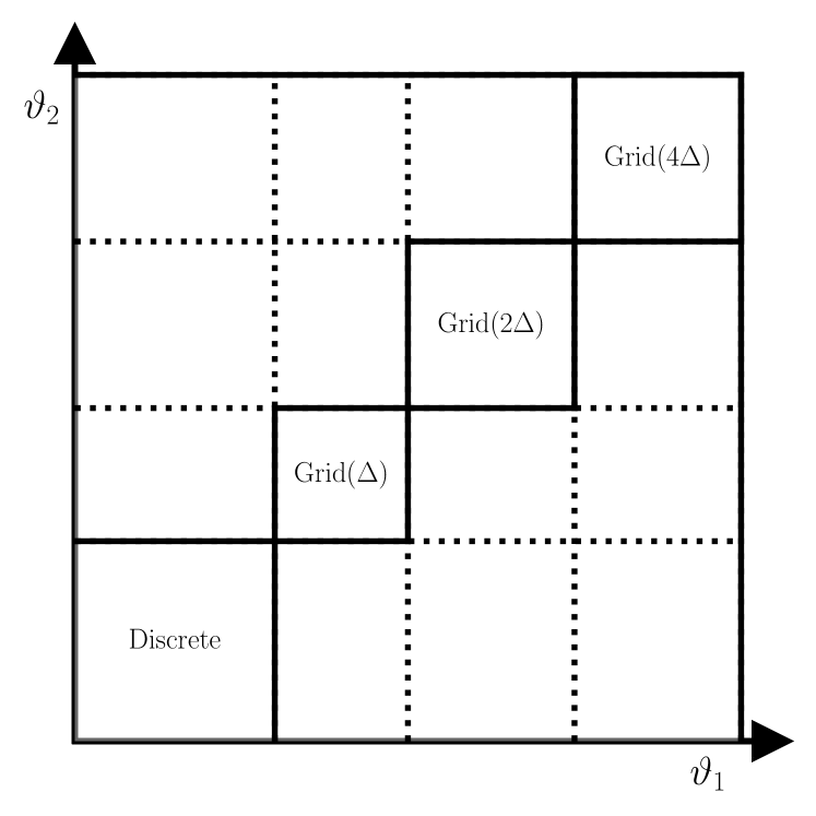
Figure 2: General strategy for computing the three-point correlators used in this work. For small angular scales, we use the prescription for discrete data to compute the Gnsubscript𝐺𝑛G_{n} and the Υi,n×subscriptsuperscriptΥ𝑖𝑛\Upsilon^{\times}_{i,n} while for larger scales, we use the grid-based approximation with varying resolution scales ΔΔ\Delta. For the off-diagonal elements, we first compute the Gnsubscript𝐺𝑛G_{n} of each radial bin using the corresponding method and then map them to the grid of the larger resolution scale from which the Υi,n×subscriptsuperscriptΥ𝑖𝑛\Upsilon^{\times}_{i,n} are obtained.

While the time complexity of the multipole estimator derived in Sect. 3.1 provides a significant speedup compared to the naive estimator and is competitive with tree-based implementations, the quadratic scaling is still prohibitive for applications in stage-IV surveys. However, we note that most of the complexity stems from the largest separations for which neighbouring galaxies make similar contributions to the Gndiscsuperscriptsubscript𝐺𝑛discG_{n}^{\mathrm{disc}} and Wndiscsuperscriptsubscript𝑊𝑛discW_{n}^{\mathrm{disc}}.444As an example, the exponential factors appearing in the Gnsubscript𝐺𝑛G_{n} and Wnsubscript𝑊𝑛W_{n} consist of 2n2𝑛2n extrema, such that for a radial bin with lower bound ΘlowsubscriptΘlow\Theta_{\mathrm{low}} galaxies separated by dΘlow/nmuch-less-than𝑑subscriptΘlow𝑛d\ll\Theta_{\mathrm{low}}/n will give similar contributions for the first n𝑛n multipoles. If one approximates the discrete ellipticity catalog by distributing the wisubscript𝑤𝑖w_{i} and the wiγc,isubscript𝑤𝑖subscript𝛾c𝑖w_{i}\gamma_{\mathrm{c}{,i}} on a regular spatial grid with pixel size ΔΔ\Delta and elements wi(Δ)subscriptsuperscript𝑤Δ𝑖w^{(\Delta)}_{i} and (wγc)i(Δ)superscriptsubscript𝑤subscript𝛾c𝑖Δ(w\gamma_{\mathrm{c}})_{i}^{(\Delta)} then for any radial bin with lower bound ΘlowΔmuch-greater-thansubscriptΘlowΔ\Theta_{\mathrm{low}}\gg\Delta this approximation will give very similar results compared to the discrete catalog. The corresponding expression for the Gnsubscript𝐺𝑛G_{n} and Wnsubscript𝑊𝑛W_{n} can now be reformulated in terms of a convolution:

GnΔ(𝜽i(Δ);Θ)superscriptsubscript𝐺𝑛Δsuperscriptsubscript𝜽𝑖ΔΘ\displaystyle G_{n}^{\Delta}\left(\boldsymbol{\theta}_{i}^{(\Delta)};\Theta\right) =k=1NpixΔ(wγc)k(Δ)einφik(Δ)(θik(Δ)Θ)absentsuperscriptsubscript𝑘1superscriptsubscript𝑁pixΔsuperscriptsubscript𝑤subscript𝛾c𝑘Δsuperscriptei𝑛superscriptsubscript𝜑𝑖𝑘Δsuperscriptsubscript𝜃𝑖𝑘ΔΘ\displaystyle=\sum_{k=1}^{N_{\mathrm{pix}}^{\Delta}}(w\gamma_{\mathrm{c}})_{k}^{(\Delta)}\ \mathrm{e}^{\mathrm{i}n\varphi_{ik}^{(\Delta)}}\ \mathcal{B}\left(\theta_{ik}^{(\Delta)}\in\Theta\right)
=[(wγc)(Δ)gn;Θ(Δ)](𝜽i(Δ)),absentdelimited-[]superscript𝑤subscript𝛾cΔsuperscriptsubscript𝑔𝑛ΘΔsuperscriptsubscript𝜽𝑖Δ\displaystyle=\left[(w\gamma_{\mathrm{c}})^{(\Delta)}\star g_{n;\Theta}^{(\Delta)}\right]\left(\boldsymbol{\theta}_{i}^{(\Delta)}\right)\ , (29)
WnΔ(𝜽i(Δ);Θ)superscriptsubscript𝑊𝑛Δsuperscriptsubscript𝜽𝑖ΔΘ\displaystyle W_{n}^{\Delta}\left(\boldsymbol{\theta}_{i}^{(\Delta)};\Theta\right) =[w(Δ)gn;Θ(Δ)](𝜽i(Δ)),absentdelimited-[]superscript𝑤Δsuperscriptsubscript𝑔𝑛ΘΔsuperscriptsubscript𝜽𝑖Δ\displaystyle=\left[w^{(\Delta)}\star g_{n;\Theta}^{(\Delta)}\right]\left(\boldsymbol{\theta}_{i}^{\left(\Delta\right)}\right)\ , (30)

where all quantities with the superscript (Δ)Δ(\Delta) are evaluated at the pixel centers and “\star” denotes the convolution operator. The transformation to multipole components Υμ,n×subscriptsuperscriptΥ𝜇𝑛\Upsilon^{\times}_{\mu,n} is equivalent to the discrete case (3.1), but the outer sum now runs over the number of pixels Npix(Δ)superscriptsubscript𝑁pixΔN_{\mathrm{pix}}^{(\Delta)} instead of the number of galaxies:

Υ0,n×(\displaystyle\Upsilon_{0,n}^{\times}( Θ1,Θ2)\displaystyle\Theta_{1},\Theta_{2})
=i=1Npix(Δ)(wγc)i(Δ)Gn3(Δ)(𝜽i(Δ);Θ1)Gn3(Δ)(𝜽i(Δ);Θ2).absentsuperscriptsubscript𝑖1superscriptsubscript𝑁pixΔsubscriptsuperscript𝑤subscript𝛾cΔ𝑖superscriptsubscript𝐺𝑛3Δsuperscriptsubscript𝜽𝑖ΔsubscriptΘ1superscriptsubscript𝐺𝑛3Δsuperscriptsubscript𝜽𝑖ΔsubscriptΘ2\displaystyle=-\sum_{i=1}^{N_{\mathrm{pix}}^{(\Delta)}}\left(w\gamma_{\mathrm{c}}\right)^{(\Delta)}_{i}\ G_{n-3}^{(\Delta)}\left(\boldsymbol{\theta}_{i}^{(\Delta)};\Theta_{1}\right)\ G_{-n-3}^{(\Delta)}\left(\boldsymbol{\theta}_{i}^{(\Delta)};\Theta_{2}\right)\ . (31)

The possibility of using FFT methods for computing the convolution gives a time complexity of the grid-based estimator of 𝒪(Npix(Δ)log(Npix(Δ)))𝒪superscriptsubscript𝑁pixΔsuperscriptsubscript𝑁pixΔ\mathcal{O}\left(N_{\mathrm{pix}}^{(\Delta)}\log\left(N_{\mathrm{pix}}^{(\Delta)}\right)\right), significantly outperforming all of the previously mentioned estimators whenever applicable.

3.3 Combined estimator

For an ellipticity catalogue from a cosmic shear survey, we can now devise an efficient estimation procedure of the shear 3PCF as depicted in Fig. 2. In the first step, we choose some scale θdiscsubscript𝜃disc\theta_{\mathrm{disc}} up until which the multipoles are computed using the discrete prescription outlined in Sect. 3.1. We then pick a base resolution scale Δ1ΔsubscriptΔ1Δ\Delta_{1}\equiv\Delta and some coarser resolutions Δd2dΔ(d=2,3,)subscriptΔ𝑑superscript2𝑑Δ𝑑23\Delta_{d}\equiv 2^{d}\Delta\ (d=2,3,...) and distribute the ellipticity catalog on the corresponding grids. For each of the scales θ>θdisc𝜃subscript𝜃disc\theta>\theta_{\mathrm{disc}} we now select some resolution Δi(θ)subscriptΔ𝑖𝜃\Delta_{i}(\theta) and compute the Gnsubscript𝐺𝑛G_{n} using the grid-based method from Sect. 3.2. To allocate the multipoles of two scales for which the Gnsubscript𝐺𝑛G_{n} were computed with different methods, the Gnsubscript𝐺𝑛G_{n} with the higher resolution need to be mapped to the coarser grid before the Υμ,n×subscriptsuperscriptΥ𝜇𝑛\Upsilon^{\times}_{\mu,n} can be updated. In particular, for the case where one of the Gnsubscript𝐺𝑛G_{n} is computed via the discrete method and the other one via the grid-based one, we first define the quantity Gn(Δ)(𝜽pi(Δ);Θ2)superscriptsubscript𝐺𝑛Δsubscriptsuperscript𝜽Δsubscript𝑝𝑖subscriptΘ2G_{n}^{\prime(\Delta)}\left(\boldsymbol{\theta}^{(\Delta)}_{p_{i}};\Theta_{2}\right) as the value of GnΔsuperscriptsubscript𝐺𝑛ΔG_{n}^{\Delta} at the pixel p𝑝p in which the i𝑖ith galaxy resides, normalized by the number of galaxies in the p𝑝pth pixel. We now have

Υ0,n×(\displaystyle\Upsilon^{\times}_{0,n}( Θ1,Θ2)\displaystyle\Theta_{1},\Theta_{2})
=i=1Ngalwiγc,iGn3disc(𝜽i;Θ1)Gn3(Δ)(𝜽pi(Δ);Θ2)absentsuperscriptsubscript𝑖1subscript𝑁galsubscript𝑤𝑖subscript𝛾c𝑖superscriptsubscript𝐺𝑛3discsubscript𝜽𝑖subscriptΘ1superscriptsubscript𝐺𝑛3Δsubscriptsuperscript𝜽Δsubscript𝑝𝑖subscriptΘ2\displaystyle=\sum_{i=1}^{N_{\mathrm{gal}}}w_{i}\gamma_{\mathrm{c},i}\ G_{n-3}^{\mathrm{disc}}(\boldsymbol{\theta}_{i};\Theta_{1})\ G_{-n-3}^{\prime(\Delta)}\left(\boldsymbol{\theta}^{(\Delta)}_{p_{i}};\Theta_{2}\right)
=p=1Npix(Δ)Gn3(Δ)(𝜽p(Δ);Θ2)i=1Ngal,p(Δ)wiγc,iGn3disc(𝜽i;Θ1)absentsuperscriptsubscript𝑝1superscriptsubscript𝑁pixΔsuperscriptsubscript𝐺𝑛3Δsubscriptsuperscript𝜽Δ𝑝subscriptΘ2superscriptsubscript𝑖1superscriptsubscript𝑁gal𝑝Δsubscript𝑤𝑖subscript𝛾c𝑖superscriptsubscript𝐺𝑛3discsubscript𝜽𝑖subscriptΘ1\displaystyle=\sum_{p=1}^{N_{\mathrm{pix}}^{(\Delta)}}G_{-n-3}^{(\Delta)}\left(\boldsymbol{\theta}^{(\Delta)}_{p};\Theta_{2}\right)\sum_{i=1}^{N_{\mathrm{gal},p}^{(\Delta)}}w_{i}\gamma_{\mathrm{c},i}\ G_{n-3}^{\mathrm{disc}}(\boldsymbol{\theta}_{i};\Theta_{1})
p=1Npix(Δ)(wγGn3disc)(Δ)(𝜽p(Δ);Θ1)Gn3(Δ)(𝜽p(Δ);Θ2),absentsuperscriptsubscript𝑝1superscriptsubscript𝑁pixΔsuperscript𝑤𝛾superscriptsubscript𝐺𝑛3discΔsubscriptsuperscript𝜽Δ𝑝subscriptΘ1superscriptsubscript𝐺𝑛3Δsubscriptsuperscript𝜽Δ𝑝subscriptΘ2\displaystyle\equiv\sum_{p=1}^{N_{\mathrm{pix}}^{(\Delta)}}\left(w\gamma G_{n-3}^{\mathrm{disc}}\right)^{(\Delta)}\left(\boldsymbol{\theta}^{(\Delta)}_{p};\Theta_{1}\right)\ G_{-n-3}^{(\Delta)}\left(\boldsymbol{\theta}^{(\Delta)}_{p};\Theta_{2}\right)\ , (32)

where the second sum in the second line runs over all Ngal,p(Δ)superscriptsubscript𝑁gal𝑝ΔN_{\mathrm{gal},p}^{(\Delta)} galaxies residing in the p𝑝pth pixel. This implies that the products wγGn3disc𝑤𝛾superscriptsubscript𝐺𝑛3discw\gamma G_{n-3}^{\mathrm{disc}} need to be evaluated at the true galaxy positions before they are mapped to the corresponding pixel. In Appendix A we give more explicit details on the time and space complexity of the combined estimator.

3.4 Edge corrections

Looking back at the general form of the estimator for the shear 3PCF (Eq. 17) we see that for a brute-force-like estimator the shear 3PCF ΓμsubscriptΓ𝜇\Gamma_{\mu} can be evaluated by a simple division of the two correlators ΥμsubscriptΥ𝜇\Upsilon_{\mu} and 𝒩𝒩\mathcal{N} for each angular- and polar bin combination. On the other hand, when working in the multipole basis we have

Γμ×(Θ1,Θ2,ϕ)=12πn=Γμ,n×(Θ1,Θ2)einϕ.subscriptsuperscriptΓ𝜇subscriptΘ1subscriptΘ2italic-ϕ12𝜋superscriptsubscript𝑛subscriptsuperscriptΓ𝜇𝑛subscriptΘ1subscriptΘ2superscriptei𝑛italic-ϕ\displaystyle\Gamma^{\times}_{\mu}(\Theta_{1},\Theta_{2},\phi)=\frac{1}{2\pi}\sum_{n=-\infty}^{\infty}\Gamma^{\times}_{\mu,n}(\Theta_{1},\Theta_{2})\ \mathrm{e}^{\mathrm{i}n\phi}\ . (33)

To work out the analog of the division in the multipole basis we first multiply Eq. (17) by 𝒩𝒩\mathcal{N} and then insert the multipole expansion of all quantities:

n,n=Γ¯μ,n×(Θ1,Θ2)superscriptsubscript𝑛superscript𝑛subscriptsuperscript¯Γ𝜇𝑛subscriptΘ1subscriptΘ2\displaystyle\sum_{n,n^{\prime}=-\infty}^{\infty}\ \overline{\Gamma}^{\times}_{\mu,n}\left({\Theta_{1},\Theta_{2}}\right)\ 𝒩n(Θ1,Θ2)ei(n+n)ϕsubscript𝒩superscript𝑛subscriptΘ1subscriptΘ2superscriptei𝑛superscript𝑛italic-ϕ\displaystyle\mathcal{N}_{n^{\prime}}(\Theta_{1},\Theta_{2})\ \mathrm{e}^{\mathrm{i}(n+n^{\prime})\phi}
=n=Υμ,n×(Θ1,Θ2)einϕ.absentsuperscriptsubscript𝑛superscriptsubscriptΥ𝜇𝑛subscriptΘ1subscriptΘ2superscriptei𝑛italic-ϕ\displaystyle=\sum_{n=-\infty}^{\infty}\Upsilon_{\mu,n}^{\times}(\Theta_{1},\Theta_{2})\ \mathrm{e}^{\mathrm{i}n\phi}\ . (34)

Multiplying Eq. (3.4) by eiϕsuperscripteiitalic-ϕ\mathrm{e}^{-\mathrm{i}\ell\phi} and integrating over ϕitalic-ϕ\phi we find:

n=𝒩n(Θ1,Θ2)Γ¯μ,n×(Θ1,Θ2)=Υμ,×(Θ1,Θ2).superscriptsubscript𝑛subscript𝒩𝑛subscriptΘ1subscriptΘ2subscriptsuperscript¯Γ𝜇𝑛subscriptΘ1subscriptΘ2superscriptsubscriptΥ𝜇subscriptΘ1subscriptΘ2\displaystyle\sum_{n=-\infty}^{\infty}\mathcal{N}_{\ell-n}(\Theta_{1},\Theta_{2})\ \overline{\Gamma}^{\times}_{\mu,n}\left({\Theta_{1},\Theta_{2}}\right)=\Upsilon_{\mu,\ell}^{\times}(\Theta_{1},\Theta_{2})\ . (35)

Thus, we see that in general there exists a coupling between different multipoles. While Eq. (35) formally describes an infinite system of equations, one expects that 𝒩nsubscript𝒩𝑛\mathcal{N}_{\ell-n} is dominated by its diagonal, such that truncating the expansion at some nmaxsubscript𝑛maxn_{\mathrm{max}} will provide a sufficient approximation.555If we assume the 3PCF to not rapidly vary over small angular scales, we expect the amplitude of the 𝒩nsubscript𝒩𝑛\mathcal{N}_{n} to approach zero for large multipoles n𝑛n. Choosing a sufficiently large nmaxsubscript𝑛maxn_{\mathrm{max}} then implies that the quantity 𝒩nsubscript𝒩𝑛\mathcal{N}_{\ell-n} will have its largest contributions for n𝑛n\approx\ell. Inverting the resulting (2nmax+1)2subscript𝑛max1(2n_{\mathrm{max}}+1) - dimensional system equips us with an expression for the edge-corrected multipoles of the shear 333PCF:

Γ¯μ,n×(Θ1,Θ2)==nmaxnmax(𝒞1)n(Θ1,Θ2)Υμ,×(Θ1,Θ2)𝒩0(Θ1,Θ2),subscriptsuperscript¯Γ𝜇𝑛subscriptΘ1subscriptΘ2superscriptsubscriptsubscript𝑛maxsubscript𝑛maxsubscriptsuperscript𝒞1𝑛subscriptΘ1subscriptΘ2subscriptsuperscriptΥ𝜇subscriptΘ1subscriptΘ2subscript𝒩0subscriptΘ1subscriptΘ2\displaystyle\overline{\Gamma}^{\times}_{\mu,n}\left({\Theta_{1},\Theta_{2}}\right)=\sum_{\ell=-n_{\mathrm{max}}}^{n_{\mathrm{max}}}{}\left(\mathcal{C}^{-1}\right)_{n\ell}(\Theta_{1},\Theta_{2})\ \frac{\Upsilon^{\times}_{\mu,\ell}(\Theta_{1},\Theta_{2})}{\mathcal{N}_{0}(\Theta_{1},\Theta_{2})}\ , (36)

where we defined the components of the mode coupling matrix 𝒞𝒞\mathcal{C} as

𝒞n(Θ1,Θ2)=𝒩n(Θ1,Θ2)𝒩0(Θ1,Θ2).subscript𝒞𝑛subscriptΘ1subscriptΘ2subscript𝒩𝑛subscriptΘ1subscriptΘ2subscript𝒩0subscriptΘ1subscriptΘ2\displaystyle\mathcal{C}_{\ell n}(\Theta_{1},\Theta_{2})=\frac{\mathcal{N}_{\ell-n}(\Theta_{1},\Theta_{2})}{\mathcal{N}_{0}(\Theta_{1},\Theta_{2})}\ . (37)

For a uniform distribution of tracers, 𝒩𝒩\mathcal{N} does not carry any angular dependence such that 𝒞𝒞\mathcal{C} becomes the identity matrix. We note that in the cosmological context, a nonuniform distribution of tracers can either be realized by a clustering of the tracers or a nontrivial survey geometry. We further note that this mode coupling effect has already been explored in Slepian & Eisenstein (2015) in the context of edge-correcting the 3PCF of scalar fields.

3.5 Including tomography

Our estimator can straightforwardly be generalized to a tomographic setting with nzsubscript𝑛𝑧n_{z} tomographic redshift bins {Zk}(k{1,,nz})subscript𝑍𝑘𝑘1subscript𝑛𝑧\{Z_{k}\}\ (k\in\{1,\cdots,n_{z}\}), where we define the galaxy at the location 𝐗isubscript𝐗𝑖\mathbf{X}_{i} in each galaxy triplet to lie in the Zisubscript𝑍𝑖Z_{i}th redshift bin. In the case of gridded data, we simply need to evaluate the GnΔsuperscriptsubscript𝐺𝑛ΔG_{n}^{\Delta} for each tomographic bin and then allocate the Υμ,n×superscriptsubscriptΥ𝜇𝑛\Upsilon_{\mu,n}^{\times} for all relevant combinations:

Υ0,n×(Θ1,Θ2;Z1,Z2,Z3)=i=1Npix(Δ)(wiγc,i)(Z1,Δ)superscriptsubscriptΥ0𝑛subscriptΘ1subscriptΘ2subscript𝑍1subscript𝑍2subscript𝑍3superscriptsubscript𝑖1superscriptsubscript𝑁pixΔsuperscriptsubscript𝑤𝑖subscript𝛾c𝑖subscript𝑍1Δ\displaystyle\Upsilon_{0,n}^{\times}(\Theta_{1},\Theta_{2};Z_{1},Z_{2},Z_{3})=-\sum_{i=1}^{N_{\mathrm{pix}}^{(\Delta)}}\left(w_{i}\gamma_{\mathrm{c},i}\right)^{(Z_{1},\Delta)}
×Gn3(Z2,Δ)(𝜽i;Θ1)Gn3(Z3,Δ)(𝜽i;Θ2),absentsuperscriptsubscript𝐺𝑛3subscript𝑍2Δsubscript𝜽𝑖subscriptΘ1superscriptsubscript𝐺𝑛3subscript𝑍3Δsubscript𝜽𝑖subscriptΘ2\displaystyle\hskip 36.98866pt\times\ G_{n-3}^{(Z_{2},\Delta)}(\boldsymbol{\theta}_{i};\Theta_{1})\ G_{-n-3}^{(Z_{3},\Delta)}(\boldsymbol{\theta}_{i};\Theta_{2})\ , (38)
Gn(Z2,Δ)(𝜽i;Θ1)=[(wγc)(Z2,Δ)gn;Θ(Δ)](𝜽i).superscriptsubscript𝐺𝑛subscript𝑍2Δsubscript𝜽𝑖subscriptΘ1delimited-[]superscript𝑤subscript𝛾csubscript𝑍2Δsuperscriptsubscript𝑔𝑛ΘΔsubscript𝜽𝑖\displaystyle G_{n}^{(Z_{2},\Delta)}(\boldsymbol{\theta}_{i};\Theta_{1})=\left[(w\gamma_{\mathrm{c}})^{(Z_{2},\Delta)}\star g_{n;\Theta}^{(\Delta)}\right](\boldsymbol{\theta}_{i})\ . (39)

For discrete data the modifications are similar, but one additionally needs to keep track of the redshift bins of both galaxies contributing to the Gnsubscript𝐺𝑛G_{n}:

Υ0,n×(Θ1,Θ2;Z1,Z2,Z3)superscriptsubscriptΥ0𝑛subscriptΘ1subscriptΘ2subscript𝑍1subscript𝑍2subscript𝑍3\displaystyle\Upsilon_{0,n}^{\times}(\Theta_{1},\Theta_{2};Z_{1},Z_{2},Z_{3}) =i=1Ngal(Z1)(wiγc,i)(Z1,Δ)absentsuperscriptsubscript𝑖1superscriptsubscript𝑁galsubscript𝑍1superscriptsubscript𝑤𝑖subscript𝛾c𝑖subscript𝑍1Δ\displaystyle=-\sum_{i=1}^{N_{\mathrm{gal}}^{(Z_{1})}}\left(w_{i}\gamma_{\mathrm{c},i}\right)^{(Z_{1},\Delta)}
×Gn3(Z2,disc)absentsuperscriptsubscript𝐺𝑛3subscript𝑍2disc\displaystyle\times\ G_{n-3}^{(Z_{2},\mathrm{disc})} (𝜽i;Θ1)Gn3(Z3,disc)(𝜽i;Θ2),subscript𝜽𝑖subscriptΘ1superscriptsubscript𝐺𝑛3subscript𝑍3discsubscript𝜽𝑖subscriptΘ2\displaystyle(\boldsymbol{\theta}_{i};\Theta_{1})\ G_{-n-3}^{(Z_{3},\mathrm{disc})}(\boldsymbol{\theta}_{i};\Theta_{2})\ , (40)
Gn(Z2,disc)(𝜽i;Θ)superscriptsubscript𝐺𝑛subscript𝑍2discsubscript𝜽𝑖Θ\displaystyle G_{n}^{(Z_{2},\mathrm{disc})}(\boldsymbol{\theta}_{i};\Theta) k=1Ngal(Z2)wkγc,kgn;Θ(𝜽ik).absentsuperscriptsubscript𝑘1superscriptsubscript𝑁galsubscript𝑍2subscript𝑤𝑘subscript𝛾c𝑘subscript𝑔𝑛Θsubscript𝜽𝑖𝑘\displaystyle\equiv\sum_{k=1}^{N_{\mathrm{gal}}^{(Z_{2})}}w_{k}\gamma_{\mathrm{c}{,k}}\ g_{n;\Theta}(\boldsymbol{\theta}_{ik})\ . (41)

The transformation to the natural components works analogously to Eq. (36).
Refer to caption
Refer to caption
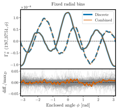
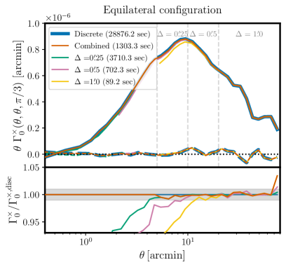
Figure 3: Performance of the combined estimator on a noiseless mock catalog with 3.1×10⁶absent3.1superscript106\approx 3.1\times 10^{6} ellipticities on a 100deg2100superscriptdegree2100\,\deg^{2} area. In the upper panels, solid lines indicate the real part of the 3PCF, while dashed lines represent the imaginary part. Left hand side: Comparison of the discrete, various grid-based, and a combined implementation of the multipole estimator for equilateral configurations of the zeroth natural component of the shear 3PCF. The timings correspond to the runtime on 888 CPU cores and the dashed vertical lines indicate the regions of constant grid resolution for the combined estimator. In the bottom panel, we show the ratios of the real parts between all approximate implementations and the discrete estimator. The grey-shaded region displays a one-per-cent interval. We note that by construction the curve corresponding to the combined estimator always lies on top of the curve corresponding to the resolution ΔdsubscriptΔ𝑑\Delta_{d} in the interval 20ΔdΘlowΘup40Δd20subscriptΔ𝑑subscriptΘlowsubscriptΘup40subscriptΔ𝑑20\Delta_{d}\leq\Theta_{\mathrm{low}}\leq\Theta_{\mathrm{up}}\leq 40\Delta_{d}. Right-hand side: Comparison of the discrete and the combined estimator for different triangle shapes. We fix two triangle sides and vary the enclosing angle ϕitalic-ϕ\phi. In the bottom panel, the thick red line shows the difference between the real part of both estimators, normalized by the largest value of the discrete estimator for the given radial bin combination maxDsubscriptmax𝐷\mathrm{max}_{D}. The grey lines display the corresponding ratios for all other radial bin combinations, where again the normalization is done with respect to the largest value of the discrete estimator for the corresponding radial bin combination.

4 Validation of the estimator

We validate our estimator on the Scinet-LIghtCone Simulations (SLICS) simulation suite (Harnois-Déraps et al. 2018). They consist of a suite of dark matter-only N-body simulations which track the evolution of 15363superscript153631536^{3} particles within a box of sidelength 505h1505superscript1505\,h^{-1}Mpc. From each simulation convergence maps are constructed up until z=3𝑧3z=3 within a field of view of 100deg2100superscriptdegree2100\,\deg^{2} on a grid of 77452superscript774527745^{2} pixels. For this work, we use the KiDS-450-like ensemble in which 819819819 fully independent ellipticity catalogs mimicking the redshift distribution and number density of the KiDS-450 data (de Jong et al. 2017) are constructed from the past light-cones. We further use a maximum multipole of nmax20subscript𝑛max20n_{\mathrm{max}}\equiv 20 for all tests presented in this and in the following section. For the remainder of this work, when transforming the shear 3PCF from its multipole basis to the real space basis, we use 100 linearly-spaced angular bins between [0,2π]02𝜋[0,2\pi], independent of the chosen value for nmaxsubscript𝑛maxn_{\mathrm{max}}.

4.1 Accuracy of the combined estimator

For testing the applicability of the grid-based approximation and the associated combined estimator we apply all of those schemes to a single noiseless mock catalog of the SLICS ensemble. In particular, we evaluate the 3PCF multipoles in 333333 log-spaced radial bins between 0.25superscriptitalic-.0250\aas@@fstack{\prime}25 and 80superscript8080^{\prime} which are then transformed to the real-space shear 3PCF. In Fig. 3 we compare the runs using the discrete estimator, the grid-based approximation for resolution scales Δ{0.25,0.5,1.0}Δsuperscriptitalic-.025superscriptitalic-.05superscriptitalic-.10\Delta\in\{0\aas@@fstack{\prime}25,0\aas@@fstack{\prime}5,1\aas@@fstack{\prime}0\}, as well as the combined estimator that uses the grid-based approximation for scales 20ΔΘlowΘup40Δ20ΔsubscriptΘlowsubscriptΘup40Δ20\Delta\leq\Theta_{\mathrm{low}}\leq\Theta_{\mathrm{up}}\leq 40\Delta and afterwards switches to the next higher resolution scale up until Δ=1Δsuperscript1\Delta=1^{\prime}.666As we define the edges of the angular bins to always contain {20Δd,40Δd}20subscriptΔ𝑑40subscriptΔ𝑑\{20\Delta_{d},40\Delta_{d}\} for all resolution scales, we do not need to consider edge cases like Θlow40ΔΘupsubscriptΘlow40ΔsubscriptΘup\Theta_{\mathrm{low}}\leq 40\Delta\Theta_{\mathrm{up}}. We note that while these bounds are not hard-coded, we will use them for the remainder of this work whenever making use of the combined estimator. For this binning scheme, the combined estimator performed 20absent20\approx 20 times faster than the discrete estimator, even outperforming the pure grid-based approximation of Δ=0.25Δsuperscriptitalic-.025\Delta=0\aas@@fstack{\prime}25. Focusing our attention on the equilateral configurations we see that the grid-based approximation is in good agreement with the discrete estimator once the separation ΘΘ\Theta is much larger than the pixelization scale ΔΔ\Delta, but it starts to bias the statistics once the separation is less than around ten times the pixelization scale. For the equilateral configurations, the combined estimator is, by construction, equal to the discrete estimator for Θ<5Θsuperscript5\Theta<5^{\prime} and then follows the measurements of the grid-based implementations. For our example shown in Fig. 3, the combined estimator is in agreement with the discrete estimator at the sub-per-cent level.

For assessing the accuracy of the blocks in the (Θ1,Θ2)subscriptΘ1subscriptΘ2(\Theta_{1},\Theta_{2})-plane shown in Fig. 2, in which the first scale is evaluated using the discrete prescription while the second scale uses the grid-based approximation, we pick one such combination of radial bins and then vary the enclosed angle ϕitalic-ϕ\phi between them. For the example shown in the right-hand panel in Fig. 3 we choose a scale for which the Gn(Δ)superscriptsubscript𝐺𝑛ΔG_{n}^{(\Delta)} are evaluated on a grid with Δ=1Δsuperscript1\Delta=1^{\prime} and we find an excellent agreement between both methods. We also show the ratios between the two schemes for all other bin combinations. Although for the majority of the curves, the ratio is very close to unity, there do appear some spikes for which the relative difference between both estimators is at the five percent level. However, those bin configurations correspond to cases in which are only a few triplets present and therefore they will not carry significant signal-to-noise in realistic data with non-vanishing shape noise.

4.2 Comparison with TREECORR
Refer to caption
Refer to caption
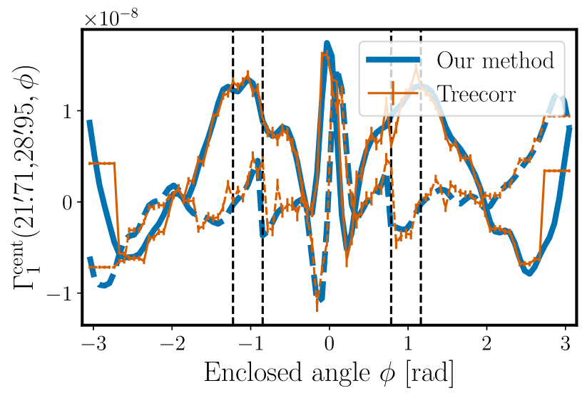
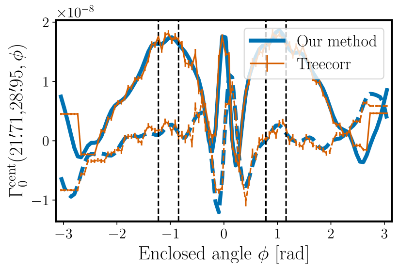
Figure 4: The first two natural components of the shear 3PCF on a catalog with 3.1×10⁵absent3.1superscript105\approx 3.1\times 10^{5} shapes on a 100deg2100superscriptdeg2100\,\mathrm{deg}^{2} area. We fix two triangle sides and vary the enclosing angle ϕitalic-ϕ\phi. Solid lines indicate the real part of the 3PCF while dashed lines stand for the imaginary part. The regions between the dashed black lines correspond to the intervals in which the ordering of the lengths of the triangle is constant. We note that due to the different binning parametrizations of TREECORR and our estimator, we do not expect perfect agreement between the curves.

The state-of-the-art method for computing shear correlation functions is based on tree codes – the most well-known implementation is the publicly available code TREECORR  (Jarvis et al. 2004)777For the tests presented in this subsection we are using version 4.2.9.. In there, the Γ¯μsubscript¯Γ𝜇\overline{\Gamma}_{\mu} are estimated by explicitly accounting for all triplets, where for an efficient evaluation, TREECORR first organizes the data in a hierarchical ball-tree structure from which the 3PCF is then computed. A further speedup can be achieved when allowing the bin edges to be fuzzy; while for reasonable values of the associated bin_slop parameter, this approximation does not bias the mean, but it increases the measurement uncertainty (Secco et al. 2022). For an efficient binning of triangle shapes TREECORR uses the quantities (r,u,v)𝑟𝑢𝑣(r,u,v) that are related to the three triangle sidelengths d1d2d3subscript𝑑1subscript𝑑2subscript𝑑3d_{1}\geq d_{2}\geq d_{3} as

r=d2;u=d3d2;v=±d1d2d3,\displaystyle r=d_{2}\ \ \ ;\ \ \ u=\frac{d_{3}}{d_{2}}\ \ \ ;\ \ \ v=\pm\frac{d_{1}-d_{2}}{d_{3}}\ , (42)

such that with u[0,1]𝑢01u\in[0,1], v[1,1]𝑣11v\in[-1,1] all triangle configurations with d1d2d3subscript𝑑1subscript𝑑2subscript𝑑3d_{1}\geq d_{2}\geq d_{3} are covered; as shown in Jarvis et al. (2004) this coverage is sufficient to obtain integrated measures of the 3PCF, such as the third-order aperture mass.

In Fig. 4 we compare the estimated components of the first two natural components Γ0,1centsubscriptsuperscriptΓcent01\Gamma^{\mathrm{cent}}_{0,1} on a single noiseless mock catalog of the SLICS ensemble. In order to facilitate an accurate matching between the two binning parametrizations one needs to use very fine bins for both estimators. For our test, we compute the 3PCF between 5superscript55^{\prime} and 50superscript5050^{\prime}, where for the multipole-based estimator we use 404040 logarithmically-spaced radial bins without making use of the grid-based approximation. For the TREECORR measurement we choose the same r𝑟r-binning and use 20(40)204020\,(40) linearly spaced bins covering the maximum range of the u(v)𝑢𝑣u\,(v) parameters. To achieve a reasonable runtime we only select every tenth galaxy, leaving a total of 3.1×10⁵absent3.1superscript105\approx 3.1\times 10^{5} ellipticities. The associated measurements were carried out on 161616 CPU cores and took 1.5absent1.5\approx 1.5 minutes for the discrete multipole-based estimator and 164absent164\approx 164 minutes for TREECORR when using a value of 0.80.80.8 for the bin_slop parameter. In Fig. 4 we find overall good agreement between both estimators across the different triangle configurations; the only significant differences are visible for strongly squeezed and folded triangles.

Besides the significantly lower computational cost compared to the tree code, the multipole-based estimator also automatically allows for a fine ϕitalic-ϕ\phi-binning of the shear 3PCF and thus provides a good approximation even for strongly degenerate triangles.888We recall that while the angular binning can be made arbitrarily small, the angular scale of the smallest features in the estimated 3PCF depends on the largest considered multipole nmaxsubscript𝑛maxn_{\mathrm{max}}. Finally, we note that the relative speedup with respect to TREECORR increases when the combined estimator is employed and when the number density of galaxies increases. For a thorough scaling analysis of the combined estimator, we again refer to Appendix A.

5 Application to third-order aperture mass measures

Due to the large size of a data vector built from an estimate of the shear 3PCF, it is unfeasible to perform a cosmological analysis using this probe. The preferred statistic is the third-order aperture mass, which provides both a compression of the data vector and a separation of the third-order shear signal in its E𝐸E- and B𝐵B-modes.

5.1 Aperture mass

The aperture mass introduced in Kaiser (1995); Schneider (1996) is a measure for the projected overdensity within a circular region of radius θ𝜃\theta around some location ϑbold-italic-ϑ\boldsymbol{\vartheta};

ap(ϑ;θ)=d2ϑUθ(|ϑ|)κ(ϑ+ϑ),subscriptapbold-italic-ϑ𝜃superscript2superscriptbold-italic-ϑsubscript𝑈𝜃superscriptbold-italic-ϑ𝜅bold-italic-ϑsuperscriptbold-italic-ϑ\displaystyle\mathcal{M}_{\mathrm{ap}}(\boldsymbol{\vartheta};\theta)=\int\differential^{2}\boldsymbol{\vartheta}^{\prime}\ U_{\theta}\left(|\boldsymbol{\vartheta}^{\prime}|\right)\ \kappa(\boldsymbol{\vartheta}+\boldsymbol{\vartheta}^{\prime})\ , (43)

where the filter function Uθsubscript𝑈𝜃U_{\theta} is compensated, meaning that aperture mass measures evade the mass-sheet degeneracy (Falco et al. 1985). Within the flat-sky approximation, the aperture mass can also be written as the real part of a complex aperture measure being defined in terms of the shear

(ϑ;θ)bold-italic-ϑ𝜃\displaystyle\mathcal{M}(\boldsymbol{\vartheta};\theta) =ap(ϑ;θ)+i×(ϑ;θ)absentsubscriptapbold-italic-ϑ𝜃isubscriptbold-italic-ϑ𝜃\displaystyle=\mathcal{M}_{\mathrm{ap}}(\boldsymbol{\vartheta};\theta)+\mathrm{i}\mathcal{M}_{\times}(\boldsymbol{\vartheta};\theta)
=d2ϑQθ(|ϑ|)γ(ϑ+ϑ;φ),absentsuperscript2superscriptbold-italic-ϑsubscript𝑄𝜃superscriptbold-italic-ϑ𝛾bold-italic-ϑsuperscriptbold-italic-ϑsuperscript𝜑\displaystyle=\int\differential^{2}\boldsymbol{\vartheta}^{\prime}\ Q_{\theta}\left(|\boldsymbol{\vartheta}^{\prime}|\right)\ \gamma(\boldsymbol{\vartheta}+\boldsymbol{\vartheta}^{\prime};\varphi^{\prime})\ , (44)

in which Qθsubscript𝑄𝜃Q_{\theta} is another filter function uniquely related to the choice of the Uθsubscript𝑈𝜃U_{\theta} filter, and φsuperscript𝜑\varphi^{\prime} denotes the polar angle of the separation vector ϑsuperscriptbold-italic-ϑ\boldsymbol{\vartheta}^{\prime}. With the aperture measure being able to separate the shear signal into its E𝐸E- and B𝐵B-modes, it can be used for both gaining cosmological information and pinning down potential systematics. For this work, we use the exponential filter introduced in Crittenden et al. (2002),

Qθ(ϑ)=ϑ24πθ4exp[(ϑ22θ2)].subscript𝑄𝜃italic-ϑsuperscriptitalic-ϑ24𝜋superscript𝜃4superscriptitalic-ϑ22superscript𝜃2\displaystyle Q_{\theta}(\vartheta)=\frac{\vartheta^{2}}{4\pi\theta^{4}}\exp[\left(-\frac{\vartheta^{2}}{2\theta^{2}}\right)]\ . (45)

5.2 Third-order aperture mass measures

The E𝐸E/B𝐵B decomposition also extends to the third-order aperture mass measures. For example, combining three aperture measures as

ap3(θ1,θ2,θ3)ap(θ1)ap(θ2)ap(θ3)delimited-⟨⟩superscriptsubscriptap3subscript𝜃1subscript𝜃2subscript𝜃3delimited-⟨⟩subscriptapsubscript𝜃1subscriptapsubscript𝜃2subscriptapsubscript𝜃3\displaystyle\left\langle\mathcal{M}_{\mathrm{ap}}^{3}\right\rangle(\theta_{1},\theta_{2},\theta_{3})\equiv\left\langle\mathcal{M}_{\mathrm{ap}}(\theta_{1})\ \mathcal{M}_{\mathrm{ap}}(\theta_{2})\ \mathcal{M}_{\mathrm{ap}}(\theta_{3})\right\rangle (46)

one can see from Eq. (43) that the resulting quantity depends on the third-order correlation function of the convergence field. By writing down the non-redundant products that appear when combining three complex measures \mathcal{M}, one obtains four real-valued quantities ap3,ap2×delimited-⟨⟩superscriptsubscriptap3delimited-⟨⟩superscriptsubscriptap2subscript\left\langle\mathcal{M}_{\mathrm{ap}}^{3}\right\rangle,\left\langle\mathcal{M}_{\mathrm{ap}}^{2}\mathcal{M}_{\times}\right\rangle, ap×2delimited-⟨⟩subscriptapsuperscriptsubscript2\left\langle\mathcal{M}_{\mathrm{ap}}\mathcal{M}_{\times}^{2}\right\rangle and ×3delimited-⟨⟩superscriptsubscript3\left\langle\mathcal{M}_{\times}^{3}\right\rangle, that are all related to a filtered version of the third-order shear correlator. Of those, only ap3delimited-⟨⟩superscriptsubscriptap3\left\langle\mathcal{M}_{\mathrm{ap}}^{3}\right\rangle carries cosmological information, while the two measures ap2×delimited-⟨⟩superscriptsubscriptap2subscript\left\langle\mathcal{M}_{\mathrm{ap}}^{2}\mathcal{M}_{\times}\right\rangle and ×3delimited-⟨⟩superscriptsubscript3\left\langle\mathcal{M}_{\times}^{3}\right\rangle vanish for parity symmetric shear fields (Schneider 2003), and a statistically significant signal of ap×2delimited-⟨⟩subscriptapsuperscriptsubscript2\left\langle\mathcal{M}_{\mathrm{ap}}\mathcal{M}_{\times}^{2}\right\rangle indicates the presence of B𝐵B-modes (Schneider et al. 2005, hereafter SKL05). Using the centroid projection Eq. (10) for the natural components SKL05 derived an explicit form of the transformation between the ΓμcensuperscriptsubscriptΓ𝜇cen\Gamma_{\mu}^{\mathrm{cen}} and the third-order aperture mass measures that are defined in terms of two third-order correlators of the complex aperture measure \mathcal{M}:

3(θ1,θ2,θ3)expectation-valuesuperscript3subscript𝜃1subscript𝜃2subscript𝜃3\displaystyle\expectationvalue{\mathcal{M}^{3}}(\theta_{1},\theta_{2},\theta_{3}) =0dϑ10dϑ202πdϕabsentsuperscriptsubscript0subscriptitalic-ϑ1superscriptsubscript0subscriptitalic-ϑ2superscriptsubscript02𝜋italic-ϕ\displaystyle=\int_{0}^{\infty}\differential\vartheta_{1}\int_{0}^{\infty}\differential\vartheta_{2}\int_{0}^{2\pi}\differential\phi
×Γ0cen(ϑ1,ϑ2,ϕ)F0(θ1,θ2,θ3;ϑ1,ϑ2,ϕ),absentsuperscriptsubscriptΓ0censubscriptitalic-ϑ1subscriptitalic-ϑ2italic-ϕsubscript𝐹0subscript𝜃1subscript𝜃2subscript𝜃3subscriptitalic-ϑ1subscriptitalic-ϑ2italic-ϕ\displaystyle\times\Gamma_{0}^{\mathrm{cen}}(\vartheta_{1},\vartheta_{2},\phi)\ F_{0}(\theta_{1},\theta_{2},\theta_{3};\vartheta_{1},\vartheta_{2},\phi)\ ,
2(θ1,θ2,θ3)expectation-valuesuperscriptsuperscript2subscript𝜃1subscript𝜃2subscript𝜃3\displaystyle\expectationvalue{\mathcal{M}^{*}\mathcal{M}^{2}}(\theta_{1},\theta_{2},\theta_{3}) =0dϑ10dϑ202πdϕabsentsuperscriptsubscript0subscriptitalic-ϑ1superscriptsubscript0subscriptitalic-ϑ2superscriptsubscript02𝜋italic-ϕ\displaystyle=\int_{0}^{\infty}\differential\vartheta_{1}\int_{0}^{\infty}\differential\vartheta_{2}\int_{0}^{2\pi}\differential\phi
×Γ1cen(ϑ1,ϑ2,ϕ)F1(θ1,θ2,θ3;ϑ1,ϑ2,ϕ),absentsuperscriptsubscriptΓ1censubscriptitalic-ϑ1subscriptitalic-ϑ2italic-ϕsubscript𝐹1subscript𝜃1subscript𝜃2subscript𝜃3subscriptitalic-ϑ1subscriptitalic-ϑ2italic-ϕ\displaystyle\times\Gamma_{1}^{\mathrm{cen}}(\vartheta_{1},\vartheta_{2},\phi)F_{1}(\theta_{1},\theta_{2},\theta_{3};\vartheta_{1},\vartheta_{2},\phi)\ , (47)

where the filter functions F0,1subscript𝐹01F_{0,1} in our convention only differ from the ones in SKL05 by cyclic permutations of the indices.999The origin of the permutation relative to the equations in SKL05 lies in the different conventions of the defining correlators of the ΓμsubscriptΓ𝜇\Gamma_{\mu} in Eq. (4). This only affects the F1subscript𝐹1F_{1} filter, as the F0subscript𝐹0F_{0} filter is symmetric under permutations of the 𝐪𝐪\mathbf{q}-vectors. We give the explicit expressions of the filters in our convention in Appendix C.

While these two correlators are sufficient for the theoretical conversion, this might not be the case when the shear 3PCF is estimated from noisy data which is distributed over several tomographic redshift bins. In this case, one needs to include two additional correlators if the full signal-to-noise should be retrieved:

(θ1,θ2,θ3)expectation-valuesuperscriptsubscript𝜃1subscript𝜃2subscript𝜃3\displaystyle\expectationvalue{\mathcal{M}\mathcal{M}^{*}\mathcal{M}}(\theta_{1},\theta_{2},\theta_{3}) =0dϑ10dϑ202πdϕabsentsuperscriptsubscript0subscriptitalic-ϑ1superscriptsubscript0subscriptitalic-ϑ2superscriptsubscript02𝜋italic-ϕ\displaystyle=\int_{0}^{\infty}\differential\vartheta_{1}\int_{0}^{\infty}\differential\vartheta_{2}\int_{0}^{2\pi}\differential\phi
×Γ2cen(ϑ1,ϑ2,ϕ)F2(θ1,θ2,θ3;ϑ1,ϑ2,ϕ),absentsuperscriptsubscriptΓ2censubscriptitalic-ϑ1subscriptitalic-ϑ2italic-ϕsubscript𝐹2subscript𝜃1subscript𝜃2subscript𝜃3subscriptitalic-ϑ1subscriptitalic-ϑ2italic-ϕ\displaystyle\times\Gamma_{2}^{\mathrm{cen}}(\vartheta_{1},\vartheta_{2},\phi)F_{2}(\theta_{1},\theta_{2},\theta_{3};\vartheta_{1},\vartheta_{2},\phi)\ ,
2(θ1,θ2,θ3)expectation-valuesuperscript2superscriptsubscript𝜃1subscript𝜃2subscript𝜃3\displaystyle\expectationvalue{\mathcal{M}^{2}\mathcal{M}^{*}}(\theta_{1},\theta_{2},\theta_{3}) =0dϑ10dϑ202πdϕabsentsuperscriptsubscript0subscriptitalic-ϑ1superscriptsubscript0subscriptitalic-ϑ2superscriptsubscript02𝜋italic-ϕ\displaystyle=\int_{0}^{\infty}\differential\vartheta_{1}\int_{0}^{\infty}\differential\vartheta_{2}\int_{0}^{2\pi}\differential\phi
×Γ3cen(ϑ1,ϑ2,ϕ)F3(θ1,θ2,θ3;ϑ1,ϑ2,ϕ).absentsuperscriptsubscriptΓ3censubscriptitalic-ϑ1subscriptitalic-ϑ2italic-ϕsubscript𝐹3subscript𝜃1subscript𝜃2subscript𝜃3subscriptitalic-ϑ1subscriptitalic-ϑ2italic-ϕ\displaystyle\times\Gamma_{3}^{\mathrm{cen}}(\vartheta_{1},\vartheta_{2},\phi)\ F_{3}(\theta_{1},\theta_{2},\theta_{3};\vartheta_{1},\vartheta_{2},\phi)\ . (48)

The individual third-order aperture mass measures then follow by a linear combination of the previous quantities; in particular, for ap3delimited-⟨⟩superscriptsubscriptap3\left\langle\mathcal{M}_{\mathrm{ap}}^{3}\right\rangle, one has:

ap3(θ1,θ2,θ3)delimited-⟨⟩superscriptsubscriptap3subscript𝜃1subscript𝜃2subscript𝜃3\displaystyle\left\langle\mathcal{M}_{\mathrm{ap}}^{3}\right\rangle(\theta_{1},\theta_{2},\theta_{3})
=Re[2(θ1,θ2,θ3)+(θ1,θ2,θ3)\displaystyle\quad\quad=\real\Large[\expectationvalue{\mathcal{M}^{2}\mathcal{M}^{*}}(\theta_{1},\theta_{2},\theta_{3})+\expectationvalue{\mathcal{M}\mathcal{M}^{*}\mathcal{M}}(\theta_{1},\theta_{2},\theta_{3})
+2(θ1,θ2,θ3)+3(θ1,θ2,θ3)]/4,\displaystyle\quad\quad\quad+\expectationvalue{\mathcal{M}^{*}\mathcal{M}^{2}}(\theta_{1},\theta_{2},\theta_{3})+\expectationvalue{\mathcal{M}^{3}}(\theta_{1},\theta_{2},\theta_{3})\Large]/4\ , (49)

and the linear combinations of the remaining aperture measures can be constructed in a similar fashion.

For a tomographic setup, the structure of the equations above remains equal, but we make the substitution

Γμcent(ϑ1,ϑ2,ϕ)Γμcent(ϑ1,ϑ2,ϕ;Z1,Z2,Z3),superscriptsubscriptΓ𝜇centsubscriptitalic-ϑ1subscriptitalic-ϑ2italic-ϕsuperscriptsubscriptΓ𝜇centsubscriptitalic-ϑ1subscriptitalic-ϑ2italic-ϕsubscript𝑍1subscript𝑍2subscript𝑍3\displaystyle\Gamma_{\mu}^{\mathrm{cent}}(\vartheta_{1},\vartheta_{2},\phi)\rightarrow\Gamma_{\mu}^{\mathrm{cent}}(\vartheta_{1},\vartheta_{2},\phi;Z_{1},Z_{2},Z_{3})\ , (50)

where the Γμcent(ϑ1,ϑ2,ϕ;Z1,Z2,Z3)superscriptsubscriptΓ𝜇centsubscriptitalic-ϑ1subscriptitalic-ϑ2italic-ϕsubscript𝑍1subscript𝑍2subscript𝑍3\Gamma_{\mu}^{\mathrm{cent}}(\vartheta_{1},\vartheta_{2},\phi;Z_{1},Z_{2},Z_{3}) are estimated as described in Sect. 3.5. This in turn means that all the other quantities, like 3expectation-valuesuperscript3\expectationvalue{\mathcal{M}^{3}} or ap3delimited-⟨⟩superscriptsubscriptap3\left\langle\mathcal{M}_{\mathrm{ap}}^{3}\right\rangle, also become functions of the tomographic redshift bin combination (Z1,Z2,Z3)subscript𝑍1subscript𝑍2subscript𝑍3(Z_{1},Z_{2},Z_{3}). We note that while the third-order aperture mass is symmetric with respect to permutations of the Zisubscript𝑍𝑖Z_{i}, this is not the case for the shear 3PCF and therefore one needs to average over all possible Zisubscript𝑍𝑖Z_{i} permutations to obtain the full signal-to-noise. We again refer to Appendix C for all explicit expressions.

5.3 Estimators of third-order aperture measures

5.3.1 Estimation via shear 3PCF

As established in the previous subsection one can estimate the third-order aperture mass measures by integrating over the 3PCF in the centroid basis. For doing this in practice we first use the multipole-based estimator (Eq. 36) introduced in Sect. 3 to obtain the shear 3PCF in the ×\times-projection, then transform them to the centroid basis via Eqs. (12-15), and finally perform the numerical integrals contained in Eq. (5.2). In Appendix E.2 we show the level of accuracy to which the 3PCF needs to be computed in order to guarantee a stable integration. As the computational bottleneck of this pipeline is the estimation of the shear 3PCF, the same computational speedup applies to the estimation of the third-order aperture measures when using the multipole-based estimator instead of traditional estimation methods of the shear 3PCF.

5.3.2 Estimation via the direct estimator

The original estimator for the third-order aperture mass statistics in simulated data on an area A𝐴A has been introduced in Schneider et al. (1998). Instead of evaluating the statistics in terms of the shear 3PCF, it directly samples third-order generalization of Eq. (5.1),

ap3(θ1,θ2,θ3)delimited-⟨⟩superscriptsubscriptap3subscript𝜃1subscript𝜃2subscript𝜃3\displaystyle\left\langle\mathcal{M}_{\mathrm{ap}}^{3}\right\rangle(\theta_{1},\theta_{2},\theta_{3}) =d2ϑAabsentsuperscript2bold-italic-ϑ𝐴\displaystyle=\int\frac{\differential^{2}\boldsymbol{\vartheta}}{A}
×i=13superscriptsubscriptproduct𝑖13\displaystyle\times\ \prod_{i=1}^{3} d2ϑiQθi(|ϑi|)γt(ϑ+ϑi;ϕi),superscript2subscriptbold-italic-ϑ𝑖subscript𝑄subscript𝜃𝑖subscriptbold-italic-ϑ𝑖subscript𝛾tbold-italic-ϑsubscriptbold-italic-ϑ𝑖subscriptitalic-ϕ𝑖\displaystyle\int\differential^{2}\boldsymbol{\vartheta}_{i}\ Q_{\theta_{i}}\left(|\boldsymbol{\vartheta}_{i}|\right)\ \gamma_{\mathrm{t}}(\boldsymbol{\vartheta}+\boldsymbol{\vartheta}_{i};\phi_{i})\ , (51)

from the ellipticities at the galaxy positions; i.e. at some angular position ϑbold-italic-ϑ\boldsymbol{\vartheta} one has

^ap3(\displaystyle\hat{\mathcal{M}}_{\mathrm{ap}}^{3}( ϑ;θ1,θ2,θ3)\displaystyle\boldsymbol{\vartheta};\theta_{1},\theta_{2},\theta_{3})
=ijkNgalwiwjwkQθ1,iQθ2,jQθ3,kγt,iγt,jγt,kijkNgalwiwjwkQθ1,iQθ2,jQθ3,k,absentsuperscriptsubscript𝑖𝑗𝑘subscript𝑁galsubscript𝑤𝑖subscript𝑤𝑗subscript𝑤𝑘subscript𝑄subscript𝜃1𝑖subscript𝑄subscript𝜃2𝑗subscript𝑄subscript𝜃3𝑘subscript𝛾t𝑖subscript𝛾t𝑗subscript𝛾t𝑘superscriptsubscript𝑖𝑗𝑘subscript𝑁galsubscript𝑤𝑖subscript𝑤𝑗subscript𝑤𝑘subscript𝑄subscript𝜃1𝑖subscript𝑄subscript𝜃2𝑗subscript𝑄subscript𝜃3𝑘\displaystyle=\frac{\sum_{i\neq j\neq k}^{N_{\mathrm{gal}}}w_{i}w_{j}w_{k}\ Q_{\theta_{1},i}Q_{\theta_{2},j}Q_{\theta_{3},k}\ \gamma_{\mathrm{t},i}\gamma_{\mathrm{t},j}\gamma_{\mathrm{t},k}}{\sum_{i\neq j\neq k}^{N_{\mathrm{gal}}}w_{i}w_{j}w_{k}\ Q_{\theta_{1},i}Q_{\theta_{2},j}Q_{\theta_{3},k}\ }\ , (52)

where we abbreviated Qθl,iQθl(|ϑiϑ|)subscript𝑄subscript𝜃𝑙𝑖subscript𝑄subscript𝜃𝑙subscriptbold-italic-ϑ𝑖bold-italic-ϑQ_{\theta_{l},i}\equiv Q_{\theta_{l}}(|\boldsymbol{\vartheta}_{i}-\boldsymbol{\vartheta}|) and γt,iγt(ϑi;ζi)subscript𝛾t𝑖subscript𝛾tsubscriptbold-italic-ϑ𝑖subscript𝜁𝑖\gamma_{\mathrm{t},i}\equiv\gamma_{\mathrm{t}}(\boldsymbol{\vartheta}_{i};\zeta_{i}) with ϑisubscriptbold-italic-ϑ𝑖\boldsymbol{\vartheta}_{i} being the angular position of the i𝑖ith galaxy and ζisubscript𝜁𝑖\zeta_{i} denoting the direction ϑiϑsubscriptbold-italic-ϑ𝑖bold-italic-ϑ\boldsymbol{\vartheta}_{i}-\boldsymbol{\vartheta}. The corresponding estimate for ap3delimited-⟨⟩superscriptsubscriptap3\left\langle\mathcal{M}_{\mathrm{ap}}^{3}\right\rangle is then obtained by covering the survey footprint with apertures and averaging over the individual estimates. As shown in Porth & Smith (2021), the nested sums appearing in Eq. (5.3.2) can be decomposed such that the estimation procedure scales linearly in the number of galaxies in the survey101010We note that, as the direct estimator assumes the apertures to be fully contained within the survey footprint, its application to a nontrivial survey geometry is not easily possible.. Although the employed Q𝑄Q-filter (45) does formally have infinite support, one can show that by only including galaxies separated by at most 4θ4𝜃4\theta from the aperture center, one recovers a practically unbiased result (Heydenreich et al. 2023). Thus, in order to avoid border effects we do not sample apertures in regions which are separated by less than 4max(θ1,θ2,θ3)4subscript𝜃1subscript𝜃2subscript𝜃34\max(\theta_{1},\theta_{2},\theta_{3}) from the fields’ boundary. We recall that while the direct estimator can be used on unmasked simulated data, like the SLICS ensemble, this is not the case for real data with a nontrivial angular survey mask.

5.4 Comparison of both estimators

We compare the results for both estimation procedures on the SLICS ensemble, using all 819 mock catalogs. We first estimate the 3PCF in the interval [0.3125,160]superscriptitalic-.03125superscript160[0\aas@@fstack{\prime}3125,160^{\prime}] using a logarithmic bin width of bΘup,i+1Θup,i=1.05𝑏subscriptΘupi1subscriptΘupi1.05b\equiv\frac{\Theta_{\mathrm{up,i+1}}}{\Theta_{\mathrm{up,i}}}=1.05. We then transform the 3PCF to the equal-scale aperture statistics, where for the aperture radii we choose 303030 logarithmically spaced values between [1,25]superscript1superscript25[1^{\prime},25^{\prime}]. Finally, we estimate ap3delimited-⟨⟩superscriptsubscriptap3\left\langle\mathcal{M}_{\mathrm{ap}}^{3}\right\rangle using the direct estimator (5.3.2) for the same set of aperture radii. In Fig. 5, we show the measurements obtained from both estimators, together with their standard deviation across the SLICS ensemble. We find a percent level agreement on aperture scales between 2superscript22^{\prime} and 10superscript1010^{\prime}; while for smaller aperture radii, the multipole-based estimator begins to yield systematically lower results, for larger aperture radii, there appears to be a scatter around the zero axis. Both of these cases are expected. On the one hand, as the shear 3PCF has not been estimated down to zero separation, the integral transformation (5.2) cannot be fully sampled for small aperture radii. Shi et al. (2014) have demonstrated that this results in a systematic underprediction of the estimated ap3delimited-⟨⟩superscriptsubscriptap3\left\langle\mathcal{M}_{\mathrm{ap}}^{3}\right\rangle for aperture radii of less than 5similar-toabsent5\sim 5 times the smallest angular separation considered in the 3PCF. For the large scales, on the other hand, one would not expect both estimators to perfectly agree with each other. Cutting off the survey boundary for the direct estimator implies that both estimators do not use the data in the same way. This can also be seen in the standard deviation of both estimators across the ensemble. While for small aperture radii, the error bars are of a similar size, the multipole-based estimator gradually extracts more signal-to-noise compared to the direct estimator for increasing aperture radii, as not all triangles can be accounted for in the latter due to the restricted sampling domain of the apertures.

6 Application to the KiDS-1000 data

6.1 The KiDS-1000 data

As a first application of our estimator to real data we use the gold sample of weak lensing and photometric redshift measurements from the fourth data release of the Kilo-Degree Survey (Kuijken et al. 2019; Wright et al. 2020; Hildebrandt et al. 2021; Giblin et al. 2021).111111The KiDS data products are public and available through https://kids.strw.leidenuniv.nl/DR4/ The gold sample consists of around 212121 million galaxies distributed over an area of 100610061006 square degrees (777777777 square degrees after masking) and is further divided into five tomographic redshift bins.

6.2 Covariance matrix
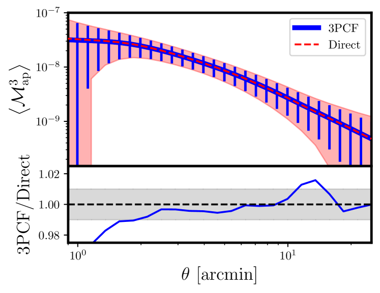
Refer to caption
Figure 5: Comparison of the third-order aperture mass statistics between the multipole-based estimator (blue line with error bars) and the direct estimator (red dashed line with error band) in the SLICS ensemble. In the lower panel, we plot the ratio between the two measurements (blue line) and show a one percent interval as the grey-shaded region.
Refer to caption
Figure 6: Correlation matrices of third-order aperture mass measures in the T17 ensemble. Shown are the results for the non-tomographic, equal-scale statistics (top left), the non-tomographic unequal-scale statistics (bottom left), as well as the tomographic equal-scale statistics (right-hand side). We order the statistics such that θiθjθksubscript𝜃𝑖subscript𝜃𝑗subscript𝜃𝑘\theta_{i}\leq\theta_{j}\leq\theta_{k} and Z1Z2Z3subscript𝑍1subscript𝑍2subscript𝑍3Z_{1}\leq Z_{2}\leq Z_{3}, meaning that each of the 352superscript35235^{2} ‘small’ squares in the covariance matrix on the right-hand side corresponds to the cross-covariance of the statistics for fixed tomographic redshift bin combinations.

We obtain an estimate for the covariance matrix by using a suite of full-sky gravitational lensing simulations introduced in Takahashi et al. (2017), hereafter the T17 ensemble. The underlying dark matter only N𝑁N-body simulations are run on a ΛΛ\LambdaCDM cosmology with Ωm=0.279subscriptΩm0.279\Omega_{\mathrm{m}}=0.279, ΩΛ=1ΩmsubscriptΩΛ1subscriptΩm\Omega_{\Lambda}=1-\Omega_{\mathrm{m}}, h=0.70.7h=0.7, σ8=0.82subscript𝜎80.82\sigma_{8}=0.82 and spectral index ns=0.97subscript𝑛s0.97n_{\mathrm{s}}=0.97. We construct 194419441944 mock ellipticity catalogs from the T17 ensemble. In particular, we match the angular positions, as well as the weights, the shape noise level per tomographic redshift bin, and the correlation between the measured ellipticities and the weights to the public KiDS-1000 ellipticity catalog (Giblin et al. 2021). We note that those specifications give rise to a different correlation structure as would be given by the SLICS ensemble, in which the galaxies are randomly placed within an unmasked area and in which each ellipticity carries an equal weight. For further details about the creation of the mocks, we refer to Burger et al. (2023).

To measure the shear 3PCF via the multipole estimator we first decompose the survey area into 161616 smaller patches. We proceed along the lines of Appendix B to measure the 3PCF multipoles in each patch and then join them after which we obtain an unbiased estimate for the third-order aperture statistics. We measure the shear 3PCF in 38 angular bins in the interval [0.75,240]superscriptitalic-.075superscript240[0\aas@@fstack{\prime}75,240^{\prime}], yielding a mean logarithmic angular bin width of b1.15𝑏1.15b\approx 1.15. The choice of the lower bound is due to the pixelization scale of underlying shear maps in the T17 ensemble, which are given in a Healpix format with nside=8192, for which the individual pixels have a side length of 0.4absentsuperscriptitalic-.04\approx 0\aas@@fstack{\prime}4. As we show in Appendix E.2, this range of angular scales yields a numerically stable transformation of the shear 3PCF to the aperture mass measures for aperture scales between 4superscript44^{\prime} and 40superscript4040^{\prime}. We do not expect that much additional information is contained in larger aperture scales, as the third-order aperture mass only filters out non-Gaussian contributions of the cosmic shear field. As we aim to obtain an accurate covariance matrix for the unequal-scale aperture statistics in the non-tomographic setup we compute the multipoles up to 303030th order in this case. For the tomographic case we only consider equal aperture scales in the measurement, for which we show in Appendix E.2 that choosing nmax=10subscript𝑛max10n_{\mathrm{max}}=10 is sufficient. Finally, we transform the shear 3PCF to the aperture statistics on two sets of radii, the ‘fine-binning set’ consisting of 303030 logarithmically-spaced radii in the interval [4,40]superscript4superscript40[4^{\prime},40^{\prime}] and the ‘coarse-binning set’ for which θ{4,6,8,10,14,18,22,26,32,36}𝜃superscript4superscript6superscript8superscript10superscript14superscript18superscript22superscript26superscript32superscript36\theta\in\{4^{\prime},6^{\prime},8^{\prime},10^{\prime},14^{\prime},18^{\prime},22^{\prime},26^{\prime},32^{\prime},36^{\prime}\}. Using these configurations the estimation of the third-order aperture measures per mock takes around 141414 hours on a single CPU for the non-tomographic case, while 4.54.54.5 hours are required on 131313 cores when including all 125125125 tomographic bin combinations for the 3PCF.

We produce mock covariance matrices for both a tomographic and a non-tomographic setup and display the resulting correlation matrices in Fig. 6. In particular, we see that the third-order aperture mass is highly correlated for radial bins of a similar angular scale. Similarly, there is a significant correlation between aperture measures being computed from different tomographic bin combinations. We will use these sample correlation matrices to assess the detection significance of the third-order aperture measures in the KiDS-1000 data.

Besides the correlation structure, we have validated that there is no significant presence of B𝐵B-modes in the mock catalogs and that the measurement of the E𝐸E-mode matches the theoretical model introduced in Heydenreich et al. (2023). We refer to Appendix D for the corresponding figure.

6.3 Measurement results

In this subsection, we present our measurement of the third-order aperture measures in the KiDS-1000 data. Throughout this subsection, we make repeated use of the ‘chi-square’

χ2=[𝐦(𝚯)𝐝]TCov1[𝐦(𝚯)𝐝],superscript𝜒2superscriptdelimited-[]𝐦𝚯𝐝𝑇superscriptCov1delimited-[]𝐦𝚯𝐝\displaystyle\chi^{2}=\left[\mathrm{\mathbf{m{(\Theta)}}-\mathbf{d}}\right]^{T}\mathrm{Cov}^{-1}\left[\mathrm{\mathbf{m{(\Theta)}}-\mathbf{d}}\right]\ , (53)

in which 𝐝𝐝\mathbf{d} denotes the data vector, CovCov\mathrm{Cov} stands for the covariance matrix of 𝐝𝐝\mathbf{d} and 𝐦(𝚯)𝐦𝚯\mathbf{m(\Theta)} is a model vector described by a set of parameters ΘΘ\Theta. As the covariance matrix is itself estimated from the T17 ensemble, we need to include the Hartlap factor (Anderson 2003; Hartlap et al. 2007) to obtain an unbiased estimate for the precision matrix Cov1superscriptCov1\mathrm{Cov}^{-1}. We quote the detection significance of 𝐝𝐝\mathbf{d} by virtue of its p𝑝p-value associated with the null hypothesis of a vanishing signal, 𝐦(𝚯)0𝐦𝚯0\mathbf{m(\Theta)}\equiv 0. Unless otherwise stated, we estimate the p𝑝p-value of some statistic measured in the KiDS-1000 data by first computing the χ2superscript𝜒2\chi^{2} for each of the 1944 mocks and then defining p𝑝p as the fraction of mocks that have a χ2superscript𝜒2\chi^{2} smaller than the χ2superscript𝜒2\chi^{2} in the real data. Finally, we introduce the signal-to-noise (S/NSN\mathrm{S/N}) of a data vector by following the definition of Secco et al. (2022):

S/N{χ2Nd.o.fifχ2>Nd.o.f+1Nullelse,SNcasessuperscript𝜒2subscript𝑁formulae-sequencedofifsuperscript𝜒2subscript𝑁formulae-sequencedof1Nullelse\displaystyle\mathrm{S/N}\equiv\begin{cases}\sqrt{\chi^{2}-N_{\mathrm{d.o.f}}}&\mathrm{if}\ \chi^{2}>N_{\mathrm{d.o.f}}+1\\ \mathrm{Null}&\mathrm{else}\end{cases}\ , (54)

where Nd.o.fsubscript𝑁formulae-sequencedofN_{\mathrm{d.o.f}} denotes the degrees-of-freedom, which for our setup is equal to the dimension of the data vector 𝐝𝐝\mathrm{\mathbf{d}}. For a thorough cosmological analysis of the measurements, we refer to Burger et al. (2023).

6.3.1 Non-tomographic measurement
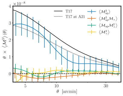
Refer to caption
Refer to caption
Figure 7: Non-tomographic third-order aperture measures in the KiDS-1000 data, using only equal aperture scales (left) or a combination of different scales (right). The error corresponds to the standard deviation in the T17 ensemble. The black solid line compares our measurement to the mean value of the T17 ensemble and the black dotted line corresponds to the result when rescaling the measurement in the T17 ensemble to a cosmology for which the values of ΩmsubscriptΩm\Omega_{\mathrm{m}} and S8subscript𝑆8S_{8} correspond to the best-fit values from A21
Refer to caption
Figure 8: Tomographic third-order aperture mass statistics in the KiDS-1000 data. In each panel, we show the measured statistics for some set of tomographic bins. The ap3superscriptsubscriptap3\mathcal{M}_{\mathrm{ap}}^{3}-signal is plotted as the blue solid line while the other solid lines indicate the remaining third-order measures. We also show the mean and the 1σ1𝜎1\sigma error interval for the third-order aperture mass within the T17 ensemble as the blue dashed line and the blue contour. The boundaries of the 1σ1𝜎1\sigma error interval for the remaining aperture measures are shown as the grey dashed and dotted curves.
Table 1: Detection significance of the third-order aperture measures for a range of setups.
Setup ndatasubscript𝑛datan_{\mathrm{data}} p𝑝p-value (no cosmic variance) p𝑝p-value S/NSN\mathrm{S/N}
ap3delimited-⟨⟩superscriptsubscriptap3\left\langle\mathcal{M}_{\mathrm{ap}}^{3}\right\rangle ap2×delimited-⟨⟩superscriptsubscriptap2subscript\left\langle\mathcal{M}_{\mathrm{ap}}^{2}\mathcal{M}_{\times}\right\rangle ap×2delimited-⟨⟩subscriptapsuperscriptsubscript2\left\langle\mathcal{M}_{\mathrm{ap}}\mathcal{M}_{\times}^{2}\right\rangle ×3delimited-⟨⟩superscriptsubscript3\left\langle\mathcal{M}_{\times}^{3}\right\rangle ap3delimited-⟨⟩superscriptsubscriptap3\left\langle\mathcal{M}_{\mathrm{ap}}^{3}\right\rangle ap3delimited-⟨⟩superscriptsubscriptap3\left\langle\mathcal{M}_{\mathrm{ap}}^{3}\right\rangle
Non-tomographic (equal θ𝜃\theta) 10 5.7×10285.7superscript10285.7\times 10^{-28} 0.90 0.09 0.26 0.05 3.19
Non-tomographic (mixed θ𝜃\theta) 20 6.5×10516.5superscript10516.5\times 10^{-51} 0.52 0.27 0.19 0.02 4.60
Tomographic (Z1=Z2=Z3subscript𝑍1subscript𝑍2subscript𝑍3Z_{1}=Z_{2}=Z_{3}) 50 4.0×1044.0superscript1044.0\times 10^{-4} 0.30 0.08 0.49 0.17 3.14
Tomographic (all) 350 9.2×10369.2superscript10369.2\times 10^{-36} 0.55 0.22 0.52 0.08 6.69
Tomographic (Zmin=2subscript𝑍min2Z_{\mathrm{min}}=2) 200 9.8×10389.8superscript10389.8\times 10^{-38} 0.38 0.87 0.50 0.11 5.32
Tomographic (Zmin=3subscript𝑍min3Z_{\mathrm{min}}=3) 100 1.6×10261.6superscript10261.6\times 10^{-26} 0.82 0.46 0.78 0.33 2.51
Tomographic (Zmin=4subscript𝑍min4Z_{\mathrm{min}}=4) 40 2.9×10212.9superscript10212.9\times 10^{-21} 0.86 0.32 0.63 0.10 3.57
Tomographic (Zmin=5subscript𝑍min5Z_{\mathrm{min}}=5) 10 1.6×1091.6superscript1091.6\times 10^{-9} 0.61 0.30 0.42 0.01 3.83
121212The second column displays the length of the data vector for each setup. The next four columns display the p𝑝p-values for the aperture measures under the assumption of no cosmological signal; in this case, the covariance for ap3delimited-⟨⟩superscriptsubscriptap3\left\langle\mathcal{M}_{\mathrm{ap}}^{3}\right\rangle does not include the cosmic variance contribution. In the final two columns, we show the p𝑝p-value and the S/NSN\mathrm{S/N} of the ap3delimited-⟨⟩superscriptsubscriptap3\left\langle\mathcal{M}_{\mathrm{ap}}^{3}\right\rangle data vector when including cosmic variance. For all but the second row only equal-scale apertures are used.

We estimate the non-tomographic third-order aperture measures in the KiDS-1000 data with the same angular binning that was used to obtain the corresponding covariance matrix in the T17 ensemble. While the figures are done using the fine-binning set, all statistical tests are performed on the coarsely binned set of aperture radii. We have further repeated the measurement using various different setups like a finer angular binning with the combined estimator, using only the discrete estimator, excluding the patch-overlap and a run using TREECORR . In all cases, we find that the measurements scatter around each other at a level of 10%similar-toabsentpercent10\sim\!10\% of the surveys’ error budget at scales 20less-than-or-similar-toabsentsuperscript20\lesssim 20^{\prime}, while for larger scales, the scatter increases a bit between the estimates utilizing the overlap between footprints and the estimators that do not. All conclusions drawn from each of the setups are the same as the ones presented below.

In Fig. 7, we show our measurement of the non-tomographic third-order aperture measures, out of which only ap3delimited-⟨⟩superscriptsubscriptap3\left\langle\mathcal{M}_{\mathrm{ap}}^{3}\right\rangle seems to be significantly different from zero. For testing the null hypothesis ‘no cosmological ap3delimited-⟨⟩superscriptsubscriptap3\left\langle\mathcal{M}_{\mathrm{ap}}^{3}\right\rangle signal’, we use the p𝑝p-value introduced above but calculate the χ2superscript𝜒2\chi^{2} using a covariance matrix that is consistent with a noise-only signal (i.e. the ×3delimited-⟨⟩superscriptsubscript3\left\langle\mathcal{M}_{\times}^{3}\right\rangle covariance matrix). In this case, we compute the p𝑝p-value using the percentile-point function of the χ2superscript𝜒2\chi^{2} distribution, which yields a value of p=5.7×1028𝑝5.7superscript1028p=5.7\times 10^{-28}, strongly rejecting the null hypothesis. Repeating this hypothesis test (but computing the p𝑝p-value as described before Eq. 54) for the remaining three modes, we find the two parity modes and the cross mode have p𝑝p-values that are consistent with a non-detection, i.e. p=0.90𝑝0.90p=0.90 for ap2×delimited-⟨⟩superscriptsubscriptap2subscript\left\langle\mathcal{M}_{\mathrm{ap}}^{2}\mathcal{M}_{\times}\right\rangle, p=0.26𝑝0.26p=0.26 for ×3delimited-⟨⟩superscriptsubscript3\left\langle\mathcal{M}_{\times}^{3}\right\rangle, and p=0.09𝑝0.09p=0.09 for ap×2delimited-⟨⟩subscriptapsuperscriptsubscript2\left\langle\mathcal{M}_{\mathrm{ap}}\mathcal{M}_{\times}^{2}\right\rangle. Besides the detection significance in the noise-only case, we can also compute the p𝑝p-value and the signal-to-noise of ap3delimited-⟨⟩superscriptsubscriptap3\left\langle\mathcal{M}_{\mathrm{ap}}^{3}\right\rangle, for which we find p=0.05𝑝0.05p=0.05 and S/N=3.19SN3.19\mathrm{S/N}=3.19. We list these values, as well as the values for all other setups described in this and the following subsection in Table 1.

When comparing the measured ap3delimited-⟨⟩superscriptsubscriptap3\left\langle\mathcal{M}_{\mathrm{ap}}^{3}\right\rangle to the mean value obtained from the T17 ensemble, we find that, while the measured ap3superscriptsubscriptap3\mathcal{M}_{\mathrm{ap}}^{3} follows a similar shape, it also has a substantially lower amplitude compared to the T17 ensemble131313We note that in the KiDS-North patch there is a relatively strong depletion of the signal on intermediate aperture scales θ[10,20,]\theta\in[10^{\prime},20,]. This also translates to the analysis of the full data set, resulting in the dip-like feature on those aperture scales visible in Fig. 7.. The majority of this discrepancy is explained by the value of σ8=0.82subscript𝜎80.82\sigma_{8}=0.82 in the T17 ensemble, which is substantially higher than the best-fit values of σ8subscript𝜎8\sigma_{8} measured in the KiDS-1000 data at the two-point level (Asgari et al. 2021, hereafter A21). Further, as the T17 ensemble was constructed from a set of discrete lens planes in the T17, the n(z)𝑛𝑧n(z) between the T17 ensemble and the KiDS-1000 data does slightly differ. To quantify the magnitude of these two effects we compute the theoretical prediction using the model of Heydenreich et al. (2023) for the T17 ensemble, as well as for a setup using the KiDS-1000 n(z)𝑛𝑧n(z) and the best-fit values for Ωm0.245subscriptΩ𝑚0.245\Omega_{m}\equiv 0.245 and S80.759subscript𝑆80.759S_{8}\equiv 0.759 from the KiDS-1000 analysis presented in A21. We then multiply the measurement in the T17 ensemble with the ratio between both theory predictions and find the resulting theoretical prediction to be in agreement with our measurement in the KiDS-1000 data (p𝑝p=0.54).

For the measurement of the unequal-scale statistics displayed in the right panel of Fig. 7, we normalize the signal by θmean(θ1θ2θ3)1/3subscript𝜃meansuperscriptsubscript𝜃1subscript𝜃2subscript𝜃313\theta_{\mathrm{mean}}\equiv\left(\theta_{1}\,\theta_{2}\,\theta_{3}\right)^{1/3} and we see similar features as in the measured equal-scale statistics, namely a slightly lower amplitude of the signal compared to the T17 ensemble. Again, we can strongly reject the null hypothesis of no cosmological ap3delimited-⟨⟩superscriptsubscriptap3\left\langle\mathcal{M}_{\mathrm{ap}}^{3}\right\rangle signal, and we also do not report a significant detection of the parity-violating modes and the cross-mode. Additionally, we see that the generalized aperture statistics has a significantly higher signal-to-noise than the equal-scale statistics (S/N=4.60)SN4.60(\mathrm{S/N}=4.60). However, we note that this does not imply much tighter cosmological constraints as the S/NSN\mathrm{S/N} measure does not take into account the dependence of the measurement on cosmological parameters. Indeed, Heydenreich et al. (2023) have demonstrated that only little cosmological information is gained by including unequal aperture scales in a non-tomographic analysis and a similar test for a tomographic setup is carried out in Burger et al. (2023), arriving at the same conclusions. Again, our measurement can be well described by the model evaluated at the A21 cosmology (p=0.48𝑝0.48p=0.48).

6.3.2 Tomographic measurement

Similar to the non-tomographic case, we present the measurement carried out using the same setup as for the covariance matrix. Again, choosing a different setup for the 3PCF computation, we draw the same conclusions. Due to computational constraints, we perform the measurement using TREECORR only on a few tomographic bin combinations, all of which yield consistent results.

Our measurement results for the 353535 non-redundant tomographic bin combinations are shown in Fig. 8. Besides the measurement, we also show the statistical uncertainty for each aperture measure, where we note that the uncertainties for ap2×delimited-⟨⟩superscriptsubscriptap2subscript\left\langle\mathcal{M}_{\mathrm{ap}}^{2}\mathcal{M}_{\times}\right\rangle and ap×2delimited-⟨⟩subscriptapsuperscriptsubscript2\left\langle\mathcal{M}_{\mathrm{ap}}\mathcal{M}_{\times}^{2}\right\rangle are equal to each other. As expected, the ap3delimited-⟨⟩superscriptsubscriptap3\left\langle\mathcal{M}_{\mathrm{ap}}^{3}\right\rangle measurements are noise-dominated for combinations of low-redshift bins, while for higher mean redshifts, the signal is significantly different from zero.

For assessing the detection significance of the aperture measures in the tomographic setup we look at the whole data vector but also perform several splits to assess potential sources of redshift-dependent systematics. In particular, we choose a data vector that only considers the auto-tomographic bin combinations, as well as a set of data vectors for which the lowest redshift bin is Zmin{2,3,4,5}subscript𝑍min2345Z_{\mathrm{min}}\ \in\{2,3,4,5\}. For all cases, we significantly rule out the null hypothesis of a non-detection of ap3delimited-⟨⟩superscriptsubscriptap3\left\langle\mathcal{M}_{\mathrm{ap}}^{3}\right\rangle, and we also do not find any significant signal for any of the remaining three measures. We refer to Table 1 for corresponding values.

6.3.3 Comparison to previous work

It is instructive to qualitatively compare our measurement to some previous results in the literature. Fu et al. (2014) have measured the non-tomographic third-order aperture statistics in the CFHTLenS data (Heymans et al. 2012) consisting of 4.24.24.2 million galaxies and a cosmological analysis has been carried out in Simon et al. (2015). Compared to our results, they do find their measured ap3delimited-⟨⟩superscriptsubscriptap3\left\langle\mathcal{M}_{\mathrm{ap}}^{3}\right\rangle signal to be in rough agreement with their mock catalogs on scales 10less-than-or-similar-toabsentsuperscript10\lesssim\!10^{\prime}. Although the error budget of the CFHTLenS survey is substantially larger than the one of KiDS-1000, they also observe a dip-like feature of the ap3delimited-⟨⟩superscriptsubscriptap3\left\langle\mathcal{M}_{\mathrm{ap}}^{3}\right\rangle signal on larger scales. They further report a significant level of ap×2delimited-⟨⟩subscriptapsuperscriptsubscript2\left\langle\mathcal{M}_{\mathrm{ap}}\mathcal{M}_{\times}^{2}\right\rangle in their measurement.

The most recent measurement of ap3delimited-⟨⟩superscriptsubscriptap3\left\langle\mathcal{M}_{\mathrm{ap}}^{3}\right\rangle has been carried out on the Y3 ellipticity catalog of the Dark Energy Survey, consisting of roughly 100100100 million galaxies (Secco et al. 2022). When comparing their non-tomographic measurement to a noiseless mock catalog constructed from one of the T17 simulations, they do not observe a dip-like feature but find a strongly depleted signal of ap3superscriptsubscriptap3\mathcal{M}_{\mathrm{ap}}^{3} relative to the mock on aperture scales of less than 10superscript1010^{\prime}. While they do not detect a significant value of ap×2delimited-⟨⟩subscriptapsuperscriptsubscript2\left\langle\mathcal{M}_{\mathrm{ap}}\mathcal{M}_{\times}^{2}\right\rangle, one can see in their Fig. 3 a similar behaviour of the ap×2delimited-⟨⟩subscriptapsuperscriptsubscript2\left\langle\mathcal{M}_{\mathrm{ap}}\mathcal{M}_{\times}^{2}\right\rangle mode on scales between 10superscript1010^{\prime} and 20superscript2020^{\prime} as in our measurement.

7 Conclusions

In this work, we presented and validated a novel estimator for the natural components of the third-order shear correlation functions and applied it to the KiDS-1000 data.

Our estimator extends the work of Slepian & Eisenstein (2015), and it builds on a multipole decomposition of the shear 3PCF for which a quadratic time complexity can be achieved when projecting the natural components of the shear 3PCF in a specific way, which we dub the ×\times-basis. We further introduced a grid-based approximation, in which the ellipticity catalog is mapped onto a regular grid, for which the 3PCF multipoles can be computed via FFT methods. We then merged both prescriptions in the ‘combined estimator’ that uses the exact computation for small angular scales, while for larger scales the grid-based approximation is employed. After including the impact of non-uniformly distributed data in the estimator, we extended the previously derived equations to a tomographic setup. We then validated our estimator and checked the applicability of the grid-based approximation on the SLICS simulation suite, for which we found that the grid-based approximation can be safely used for angular separations of at least 202020 times the pixel scale. We furthermore compared our estimator against the state-of-the-art estimation method TREECORR and found an excellent agreement between both approaches with the multipole-based approach providing a speedup of several orders of magnitude. Following a short review of how to numerically obtain the third-order aperture measures from the shear 3PCF, we validated our numerical implementation of this transformation against the direct estimator, finding a sub-percent-level agreement when using a logarithmic radial bin width b=1.05𝑏1.05b=1.05 for the 3PCF estimation.

Next, we proceeded to the measurement of the third-order aperture measures in the KiDS-1000 data. We constructed a suite of 194419441944 mock ellipticity catalogs from the T17 ray-tracing simulations from which we computed a sample covariance matrix that includes the effect of the KiDS-1000 footprint, the angular distribution of the galaxies, as well as the correlation between the galaxy weights and the measured shapes. For the non-tomographic analysis, we reported a significant detection of a cosmological ap3delimited-⟨⟩superscriptsubscriptap3\left\langle\mathcal{M}_{\mathrm{ap}}^{3}\right\rangle signal and also found that the parity-violating modes, as well as the cross mode were consistent with a non-detection. For the tomographic analysis, we again report a significant detection of the ap3delimited-⟨⟩superscriptsubscriptap3\left\langle\mathcal{M}_{\mathrm{ap}}^{3}\right\rangle signal while none of the remaining three modes had a suspiciously low p𝑝p-value. Finally, we qualitatively compared our measurement results against previous measurements in the CFHTLenS and the DES-Y3 data.

We have demonstrated that a multipole-based estimator of the shear 3PCF provides accurate results in a fraction of the time of state-of-the-art estimation procedures. This will make it feasible to utilize these methods for measuring a third-order signal in forthcoming stage-IV surveys and for constructing an accurate numerical covariance matrix taking into account all survey specifics. Extensions of these methods to higher orders are conceptually straightforward though technically cumbersome, and we leave them to future work.

Acknowledgements.
This paper went through the KiDS review process, where we want to thank the KiDS internal reviewer and Joachim Harnois-Déraps for useful comments. The figures in this work were created with matplotlib (Hunter 2007) Some of the results in this paper have been derived using the healpy and HEALPix141414currently http://healpix.sourceforge.net package (Górski et al. 2005; Zonca et al. 2019). We further make use of the numpy (Harris et al. 2020) and scipy (Virtanen et al. 2020) software packages. LP acknowledges support from the DLR grant 50QE2002. SH is supported by the U.D Department of Energy, Office of Science, Office of High Energy Physics under Award Number DE-SC0019301. LL is supported by the Austrian Science Fund (FWF) [ESP 357-N]. We acknowledge use of the lux supercomputer at UC Santa Cruz, funded by NSF MRI grant AST 1828315.
Author contributions: All authors contributed to the development and writing of this paper.
Some results in this paper are based on observations made with ESO Telescopes at the La Silla Paranal Observatory under programme IDs 177.A-3016, 177.A-3017, 177.A-3018 and 179.A-2004, and on data products produced by the KiDS consortium. The KiDS production team acknowledges support from: Deutsche Forschungsgemeinschaft, ERC, NOVA and NWO-M grants; Target; the University of Padova, and the University Federico II (Naples).

References

  • Amon et al. (2022) Amon, A., Gruen, D., Troxel, M. A., et al. 2022, Phys. Rev. D, 105, 023514
  • Anderson (2003) Anderson, T. 2003, An Introduction to Multivariate Statistical Analysis, Wiley Series in Probability and Statistics (Wiley)
  • Asgari et al. (2021) Asgari, M., Lin, C.-A., Joachimi, B., et al. 2021, A&A, 645, A104
  • Bartelmann & Schneider (2001) Bartelmann, M. & Schneider, P. 2001, Phys. Rep, 340, 291
  • Barthelemy et al. (2020) Barthelemy, A., Codis, S., Uhlemann, C., Bernardeau, F., & Gavazzi, R. 2020, MNRAS, 492, 3420
  • Bernardeau et al. (2002) Bernardeau, F., Mellier, Y., & van Waerbeke, L. 2002, A&A, 389, L28
  • Boyle et al. (2021) Boyle, A., Uhlemann, C., Friedrich, O., et al. 2021, MNRAS, 505, 2886
  • Burger et al. (2023) Burger, P., Porth, L., Schneider, P., et al. 2023, submitted to A&A, and published on arXiv
  • Chen & Szapudi (2005) Chen, G. & Szapudi, I. 2005, ApJ, 635, 743
  • Crittenden et al. (2002) Crittenden, R. G., Natarajan, P., Pen, U.-L., & Theuns, T. 2002, ApJ, 568, 20
  • Dalal et al. (2023) Dalal, R., Li, X., Nicola, A., et al. 2023, arXiv e-prints, arXiv:2304.00701
  • de Jong et al. (2017) de Jong, J. T. A., Verdoes Kleijn, G. A., Erben, T., et al. 2017, A&A, 604, A134
  • Dodelson (2017) Dodelson, S. 2017, Gravitational Lensing (Cambridge University Press)
  • Falco et al. (1985) Falco, E. E., Gorenstein, M. V., & Shapiro, I. I. 1985, ApJ, 289, L1
  • Fu et al. (2014) Fu, L., Kilbinger, M., Erben, T., et al. 2014, MNRAS, 441, 2725
  • Gatti et al. (2020) Gatti, M., Chang, C., Friedrich, O., et al. 2020, MNRAS, 498, 4060
  • Giblin et al. (2023) Giblin, B., Cai, Y.-C., & Harnois-Déraps, J. 2023, MNRAS, 520, 1721
  • Giblin et al. (2021) Giblin, B., Heymans, C., Asgari, M., et al. 2021, A&A, 645, A105
  • Górski et al. (2005) Górski, K. M., Hivon, E., Banday, A. J., et al. 2005, ApJ, 622, 759
  • Hamana et al. (2020) Hamana, T., Shirasaki, M., Miyazaki, S., et al. 2020, PASJ, 72, 16
  • Hamana et al. (2004) Hamana, T., Takada, M., & Yoshida, N. 2004, MNRAS, 350, 893
  • Harnois-Déraps et al. (2018) Harnois-Déraps, J., Amon, A., Choi, A., et al. 2018, MNRAS, 481, 1337
  • Harnois-Déraps et al. (2021) Harnois-Déraps, J., Martinet, N., Castro, T., et al. 2021, MNRAS, 506, 1623
  • Harris et al. (2020) Harris, C. R., Millman, K. J., van der Walt, S. J., et al. 2020, Nature, 585, 357
  • Hartlap et al. (2007) Hartlap, J., Simon, P., & Schneider, P. 2007, A&A, 464, 399
  • Heydenreich et al. (2022) Heydenreich, S., Brück, B., Burger, P., et al. 2022, A&A, 667, A125
  • Heydenreich et al. (2023) Heydenreich, S., Linke, L., Burger, P., & Schneider, P. 2023, A&A, 672, A44
  • Heymans et al. (2013) Heymans, C., Grocutt, E., Heavens, A., et al. 2013, MNRAS, 432, 2433
  • Heymans et al. (2012) Heymans, C., Van Waerbeke, L., Miller, L., et al. 2012, MNRAS, 427, 146
  • Hikage et al. (2019) Hikage, C., Oguri, M., Hamana, T., et al. 2019, PASJ, 71, 43
  • Hildebrandt et al. (2021) Hildebrandt, H., van den Busch, J. L., Wright, A. H., et al. 2021, A&A, 647, A124
  • Hildebrandt et al. (2017) Hildebrandt, H., Viola, M., Heymans, C., et al. 2017, MNRAS, 465, 1454
  • Hou et al. (2022) Hou, J., Slepian, Z., & Cahn, R. N. 2022, arXiv:2206.03625
  • Hunter (2007) Hunter, J. D. 2007, Computing in Science & Engineering, 9, 90
  • Ivezić et al. (2019) Ivezić, Ž., Kahn, S. M., Tyson, J. A., et al. 2019, ApJ, 873, 111
  • Jain & Seljak (1997) Jain, B. & Seljak, U. 1997, ApJ, 484, 560
  • Jarvis et al. (2004) Jarvis, M., Bernstein, G., & Jain, B. 2004, MNRAS, 352, 338
  • Kaiser (1995) Kaiser, N. 1995, ApJ, 439, L1
  • Kilbinger (2015) Kilbinger, M. 2015, Reports on Progress in Physics, 78, 086901
  • Kilbinger et al. (2014) Kilbinger, M., Bonnett, C., & Coupon, J. 2014, athena: Tree code for second-order correlation functions, Astrophysics Source Code Library, record ascl:1402.026
  • Kilbinger & Schneider (2005) Kilbinger, M. & Schneider, P. 2005, A&A, 442, 69
  • Kratochvil et al. (2012) Kratochvil, J. M., Lim, E. A., Wang, S., et al. 2012, Phys. Rev. D, 85, 103513
  • Kruse & Schneider (1999) Kruse, G. & Schneider, P. 1999, MNRAS, 302, 821
  • Kuijken et al. (2019) Kuijken, K., Heymans, C., Dvornik, A., et al. 2019, A&A, 625, A2
  • Laureijs et al. (2011) Laureijs, R., Amiaux, J., Arduini, S., et al. 2011, arXiv:1110.3193
  • Li et al. (2023) Li, X., Zhang, T., Sugiyama, S., et al. 2023, arXiv:2304.00702
  • Linke et al. (2023) Linke, L., Heydenreich, S., Burger, P. A., & Schneider, P. 2023, A&A, 672, A185
  • Mandelbaum (2018) Mandelbaum, R. 2018, ARA&A, 56, 393
  • Parroni et al. (2020) Parroni, C., Cardone, V. F., Maoli, R., & Scaramella, R. 2020, A&A, 633, A71
  • Patton et al. (2017) Patton, K., Blazek, J., Honscheid, K., et al. 2017, MNRAS, 472, 439
  • Philcox (2022) Philcox, O. H. E. 2022, Phys. Rev. D, 106, 063501
  • Philcox et al. (2022) Philcox, O. H. E., Slepian, Z., Hou, J., et al. 2022, MNRAS, 509, 2457
  • Porth & Smith (2021) Porth, L. & Smith, R. E. 2021, MNRAS, 508, 3474
  • Pyne & Joachimi (2021) Pyne, S. & Joachimi, B. 2021, MNRAS, 503, 2300
  • Schneider (1996) Schneider, P. 1996, MNRAS, 283, 837
  • Schneider (2003) Schneider, P. 2003, A&A, 408, 829
  • Schneider et al. (2005) Schneider, P., Kilbinger, M., & Lombardi, M. 2005, A&A, 431, 9
  • Schneider & Lombardi (2003) Schneider, P. & Lombardi, M. 2003, A&A, 397, 809
  • Schneider et al. (1998) Schneider, P., van Waerbeke, L., Jain, B., & Kruse, G. 1998, MNRAS, 296, 873
  • Secco et al. (2022) Secco, L. F., Jarvis, M., Jain, B., et al. 2022, Phys. Rev. D, 105, 103537
  • Semboloni et al. (2008) Semboloni, E., Heymans, C., van Waerbeke, L., & Schneider, P. 2008, MNRAS, 388, 991
  • Semboloni et al. (2011) Semboloni, E., Schrabback, T., van Waerbeke, L., et al. 2011, MNRAS, 410, 143
  • Shi et al. (2014) Shi, X., Joachimi, B., & Schneider, P. 2014, A&A, 561, A68
  • Simon et al. (2015) Simon, P., Semboloni, E., van Waerbeke, L., et al. 2015, MNRAS, 449, 1505
  • Slepian & Eisenstein (2015) Slepian, Z. & Eisenstein, D. J. 2015, MNRAS, 454, 4142
  • Takada & Jain (2003) Takada, M. & Jain, B. 2003, MNRAS, 340, 580
  • Takahashi et al. (2017) Takahashi, R., Hamana, T., Shirasaki, M., et al. 2017, ApJ, 850, 24
  • Takahashi et al. (2020) Takahashi, R., Nishimichi, T., Namikawa, T., et al. 2020, ApJ, 895, 113
  • Troxel et al. (2018) Troxel, M. A., MacCrann, N., Zuntz, J., et al. 2018, Phys. Rev. D, 98, 043528
  • Vicinanza et al. (2018) Vicinanza, M., Cardone, V. F., Maoli, R., Scaramella, R., & Er, X. 2018, Phys. Rev. D, 97, 023519
  • Virtanen et al. (2020) Virtanen, P., Gommers, R., Oliphant, T. E., et al. 2020, Nature Methods, 17, 261
  • Wright et al. (2020) Wright, A. H., Hildebrandt, H., van den Busch, J. L., & Heymans, C. 2020, A&A, 637, A100
  • Zaldarriaga & Scoccimarro (2003) Zaldarriaga, M. & Scoccimarro, R. 2003, ApJ, 584, 559
  • Zhang & Pen (2005) Zhang, L. L. & Pen, U.-L. 2005, New A, 10, 569
  • Zonca et al. (2019) Zonca, A., Singer, L., Lenz, D., et al. 2019, Journal of Open Source Software, 4, 1298

Appendix A Additional implementation specifics and scaling
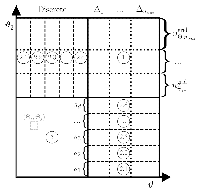
Refer to caption
Figure 9: Decomposition of the (ϑ1,ϑ2)subscriptitalic-ϑ1subscriptitalic-ϑ2(\vartheta_{1},\vartheta_{2})-plane used for our implementation of the combined estimator. The grid itself is tiled into nΘ2superscriptsubscript𝑛Θ2n_{\Theta}^{2} elements, each corresponding to a combination of angular bins (Θi,Θj)subscriptΘ𝑖subscriptΘ𝑗(\Theta_{i},\Theta_{j}) and each of those elements falls into one of the blocks 1, 2.i or 3.

A.1 Notation and high-level overview

In this appendix we look at the time- and space complexity of the combined estimator. For the remainder of this section, we assume a patch of Ngsubscript𝑁gN_{\mathrm{g}} galaxies sampled at density n¯¯𝑛\overline{n} across nzsubscript𝑛zn_{\mathrm{z}} tomographic bins and we furthermore assume that we are interested in measuring all multipole components such that we can evaluate the 3PCF (Eq. 36) between the zeroth and the nmaxsubscript𝑛maxn_{\mathrm{max}}th multipole on nΘsubscript𝑛Θn_{\Theta} radial bins. We additionally assume that we choose a strategy in which we compute the first (smallest) nΘdiscsuperscriptsubscript𝑛Θdiscn_{\Theta}^{\mathrm{disc}} radial bins using the discrete estimator while the remaining nΘgridnΘnΘdiscsuperscriptsubscript𝑛Θgridsubscript𝑛Θsuperscriptsubscript𝑛Θdiscn_{\Theta}^{\mathrm{grid}}\equiv n_{\Theta}-n_{\Theta}^{\mathrm{disc}} radial bins are computed using the grid-based estimator with nresosubscript𝑛reson_{\mathrm{reso}} resolutions Δi2i1Δ1subscriptΔ𝑖superscript2𝑖1subscriptΔ1\Delta_{i}\equiv 2^{i-1}\Delta_{1} for which the original ellipticity catalog is mapped to Npix(Δi)superscriptsubscript𝑁pixsubscriptΔ𝑖N_{\mathrm{pix}}^{(\Delta_{i})} nonempty pixels and for each resolution scale nΘ,igridsuperscriptsubscript𝑛Θ𝑖gridn_{\Theta,i}^{\mathrm{grid}} radial bins are used, such that i=1nresonΘ,igrid=nΘgridsuperscriptsubscript𝑖1subscript𝑛resosuperscriptsubscript𝑛Θ𝑖gridsuperscriptsubscript𝑛Θgrid\sum_{i=1}^{n_{\mathrm{reso}}}n_{\Theta,i}^{\mathrm{grid}}=n_{\Theta}^{\mathrm{grid}}. For later convenience, we also define a partition of the set of discrete radii into sets of (s1,sd)subscript𝑠1subscript𝑠𝑑({s}_{1},\cdots{s}_{d}) subintervals of size sisubscript𝑠𝑖{s}_{i}.

To ensure a good compromise between the time- and space complexity of the estimator, we decompose the (Θ1,Θ2)subscriptΘ1subscriptΘ2(\Theta_{1},\Theta_{2})-plane into several blocks as shown in Fig. 9 and calculate them in the following order: For the first block (gg-block) 1 we calculate the multipoles in which both ΘΘ\Theta-bins are computed using the grid-based approximation. We then compute the second blocks (gd-blocks) 2 that consist of the multipoles for which only one of the ΘΘ\Theta-bins is computed using the grid-based approximation while the other one uses the discrete method. Since in most applications, this step consumes the most memory we subdivide this block into d𝑑d sub-blocks 2.i only using sisubscript𝑠𝑖{s}_{i} elements from the discrete bins. Finally, for the third block (dd-block) 3.1 we compute the remaining multipoles using the discrete prescription and then allocate the last gd-block 2.d.

A.2 Time complexity

For step 1 the time complexity is of order151515In this subsection we only mention contributions to the time- and space complexity that can become dominant for a given survey and measurement setup.

nmaxnzi=1nresonΘ,igrid𝒪[Npix(Δi)log(Npix(Δi))]subscript𝑛maxsubscript𝑛𝑧superscriptsubscript𝑖1subscript𝑛resosuperscriptsubscript𝑛Θ𝑖grid𝒪delimited-[]superscriptsubscript𝑁pixsubscriptΔ𝑖superscriptsubscript𝑁pixsubscriptΔ𝑖\displaystyle n_{\mathrm{max}}\ \ n_{z}\ \ \sum_{i=1}^{n_{\mathrm{reso}}}n_{\Theta,i}^{\mathrm{grid}}\ \mathcal{O}\left[N_{\mathrm{pix}}^{(\Delta_{i})}\ \log\left(N_{\mathrm{pix}}^{(\Delta_{i})}\right)\right]
+nmaxnz3i=1nreso{[(nΘ,igrid)2+2(nΘ,igridj=1i1nΘ,jgrid)]𝒪(Npix(Δi))},subscript𝑛maxsuperscriptsubscript𝑛𝑧3superscriptsubscript𝑖1subscript𝑛resodelimited-[]superscriptsuperscriptsubscript𝑛Θ𝑖grid22superscriptsubscript𝑛Θ𝑖gridsuperscriptsubscript𝑗1𝑖1superscriptsubscript𝑛Θ𝑗grid𝒪superscriptsubscript𝑁pixsubscriptΔ𝑖\displaystyle+\ \ n_{\mathrm{max}}\ \ n_{z}^{3}\ \ \sum_{i=1}^{n_{\mathrm{reso}}}\left\{\left[\left(n_{\Theta,i}^{\mathrm{grid}}\right)^{2}+2\left(n_{\Theta,i}^{\mathrm{grid}}\sum_{j=1}^{i-1}n_{\Theta,j}^{\mathrm{grid}}\right)\right]\ \mathcal{O}\left(N_{\mathrm{pix}}^{(\Delta_{i})}\right)\right\}\ , (55)

where the terms in the first line correspond to the computation of the Gn(Δi)superscriptsubscript𝐺𝑛subscriptΔ𝑖G_{n}^{(\Delta_{i})} via FFTs and the second line concerns the time taken to average them to obtain the multipole components. In particular, the first term in the second line considers the blocks in which the resolution scales are equal while the second term in the second line runs over all remaining terms contained in 1. Noting that Npix(Δi+1)0.25Npix(Δi)superscriptsubscript𝑁pixsubscriptΔ𝑖10.25superscriptsubscript𝑁pixsubscriptΔ𝑖N_{\mathrm{pix}}^{(\Delta_{i+1})}\approx 0.25\,N_{\mathrm{pix}}^{(\Delta_{i})}, these expressions show the time benefit of using coarser grid resolutions for large radial separations.161616In our implementation the prefactor is slightly larger than 0.250.250.25 as for each resolution scale we filter out empty pixels, guaranteeing that Npix(Δ1)Ngalsuperscriptsubscript𝑁pixsubscriptΔ1subscript𝑁galN_{\mathrm{pix}}^{(\Delta_{1})}\leq N_{\mathrm{gal}} for any resolution scale. We note that both terms scale differently in the number of radial and tomographic bins; while for a coarse radial binning and a non-tomographic setup, the first term dominates, this is not true in general when the additional prefactors in the second term surpass the additional logarithmic contribution in the first term.

The time complexity for each of the 2.i is

nmaxn¯subscript𝑛max¯𝑛\displaystyle n_{\mathrm{max}}\ \overline{n} (Θsi,up2Θsi,low2)𝒪(Ng)+limit-fromsuperscriptsubscriptΘsubscript𝑠𝑖up2superscriptsubscriptΘsubscript𝑠𝑖low2𝒪subscript𝑁g\displaystyle\left(\Theta_{{s}_{i},\mathrm{up}}^{2}-\Theta_{{s}_{i},\mathrm{low}}^{2}\right)\ \mathcal{O}\left(N_{\mathrm{g}}\right)+
nmaxnz3sii=1nresonΘ,igrid𝒪(Npix(Δi)),subscript𝑛maxsuperscriptsubscript𝑛𝑧3subscript𝑠𝑖superscriptsubscript𝑖1subscript𝑛resosuperscriptsubscript𝑛Θ𝑖grid𝒪superscriptsubscript𝑁pixsubscriptΔ𝑖\displaystyle n_{\mathrm{max}}\ \ n_{z}^{3}\ \ {s}_{i}\ \ \sum_{i=1}^{n_{\mathrm{reso}}}n_{\Theta,i}^{\mathrm{grid}}\ \mathcal{O}\left(N_{\mathrm{pix}}^{(\Delta_{i})}\right)\ , (56)

where both lines correspond to the same operations as the ones in Eq. (A.2). We note that the nmaxsubscript𝑛maxn_{\mathrm{max}} factor in the first line is well approximated with unity as in the construction of the Gndiscsuperscriptsubscript𝐺𝑛discG_{n}^{\mathrm{disc}} in Eq. (3.1) only requires a single evaluation of the complex exponential from which all values for n𝑛n can be inferred by a few addition and multiplication operations. We further note that between two different sub-intervals sisubscript𝑠𝑖{s}_{i}, sjsubscript𝑠𝑗{s}_{j} both terms consist of fully complementary computations and that the second line effectively scales as if the ellipticities were distributed on regular grids.

For the first part of the final step 3 we have

nmax[(n¯Θsd,up2)+nz2(nΘdisc)2]𝒪(Ng)subscript𝑛max¯𝑛superscriptsubscriptΘsubscript𝑠𝑑up2superscriptsubscript𝑛𝑧2superscriptsuperscriptsubscript𝑛Θdisc2𝒪subscript𝑁g\displaystyle n_{\mathrm{max}}\ \left[\ \left(\overline{n}\ \Theta_{{s}_{d},\mathrm{up}}^{2}\right)\ \ \ +\ \ \ n_{z}^{2}\ \ \left(n_{\Theta}^{\mathrm{disc}}\right)^{2}\right]\ \mathcal{O}\left(N_{\mathrm{g}}\right) (57)

in which both terms can be interpreted similarly to the scaling of 2.i, but the second term is scaling only quadratically in terms of the number of z𝑧z-bins, as one would expect from Eq. (3.5).

The computation of the final gd-block 2.d is equal to the formal scaling of the second line in Eq. (A.2). We note that the first term in Eq. (57) is the only step in the method for which calculations are repeated, namely the allocation of the Gndiscsuperscriptsubscript𝐺𝑛discG_{n}^{\mathrm{disc}} in the interval [Θs0,low,Θsd,low]subscriptΘsubscript𝑠0lowsubscriptΘsubscript𝑠𝑑low[\Theta_{{s}_{0},\mathrm{low}},\Theta_{{s}_{d},\mathrm{low}}]. For most realistic cases Θsd,low0.5Θsd,upless-than-or-similar-tosubscriptΘsubscript𝑠𝑑low0.5subscriptΘsubscript𝑠𝑑up\Theta_{{s}_{d},\mathrm{low}}\lesssim 0.5\,\Theta_{{s}_{d},\mathrm{up}}, meaning that the repeated calculations only constitute a subdominant fraction of the time complexity.

A.3 Space complexity

From the observation that the time complexity of the computation of the Gndiscsuperscriptsubscript𝐺𝑛discG_{n}^{\mathrm{disc}} is dominated by the computation of the first value G1subscript𝐺1G_{1}, we aim to allocate the Υμ,n×subscriptsuperscriptΥ𝜇𝑛\Upsilon^{\times}_{\mu,n} for all multipole orders at once. This implies that for the allocation of the gd-blocks one needs to keep all relevant GnΔisuperscriptsubscript𝐺𝑛subscriptΔ𝑖G_{n}^{\Delta_{i}} in memory - the corresponding space complexity is of order

nmaxnzi=1nresonΘ,igrid𝒪(Npix(Δi)).subscript𝑛maxsubscript𝑛𝑧superscriptsubscript𝑖1subscript𝑛resosuperscriptsubscript𝑛Θ𝑖grid𝒪superscriptsubscript𝑁pixsubscriptΔ𝑖\displaystyle n_{\mathrm{max}}\ \ n_{z}\ \ \sum_{i=1}^{n_{\mathrm{reso}}}n_{\Theta,i}^{\mathrm{grid}}\ \mathcal{O}\left(N_{\mathrm{pix}}^{(\Delta_{i})}\right)\ . (58)

Additionally, from Eq. (3.3) follows the requirement to map the wγcGndisc𝑤subscript𝛾csuperscriptsubscript𝐺𝑛discw\gamma_{\mathrm{c}}\ G_{n}^{\mathrm{disc}} to grids of the corresponding pixel resolutions which results in a memory footprint of order

nmaxnz2nΘdisci=1nreso𝒪(Npix(Δi)).subscript𝑛maxsuperscriptsubscript𝑛𝑧2superscriptsubscript𝑛Θdiscsuperscriptsubscript𝑖1subscript𝑛reso𝒪superscriptsubscript𝑁pixsubscriptΔ𝑖\displaystyle n_{\mathrm{max}}\ n_{z}^{2}\ \ n_{\Theta}^{\mathrm{disc}}\ \ \sum_{i=1}^{n_{\mathrm{reso}}}\mathcal{O}\left(N_{\mathrm{pix}}^{(\Delta_{i})}\right)\ . (59)

In almost all cases, this term has the largest memory contribution171717For example, for nmax=30subscript𝑛max30n_{\mathrm{max}}=30, nz=5subscript𝑛𝑧5n_{z}=5, nΘdisc=20superscriptsubscript𝑛Θdisc20n_{\Theta}^{\mathrm{disc}}=20 and a cumulative sum of reduced pixels i=1dNpix(Δi)superscriptsubscript𝑖1𝑑superscriptsubscript𝑁pixsubscriptΔ𝑖\sum_{i=1}^{d}N_{\mathrm{pix}}^{(\Delta_{i})} of order 106superscript10610^{6} one finds, after restoring constant prefactors, a memory requirement of 4.7×10⁹absent4.7superscript109\approx 4.7\times 10^{9} complex-valued entries., which lead to our subdivision of this step into d𝑑d substeps only requiring 1/d1𝑑1/d-th part of the memory while leaving the time complexity nearly untouched.

Finally, the storage requirement of the computed 3PCF multipoles is 5(nmax+1)nΘ2nz35subscript𝑛max1superscriptsubscript𝑛Θ2superscriptsubscript𝑛𝑧35\,(n_{\mathrm{max}}+1)\ n_{\Theta}^{2}\ n_{z}^{3} complex-valued entries, where we made use of the symmetries

Υ0,n×(Θi,Θj;Zk,Zl,Zm)subscriptsuperscriptΥ0𝑛subscriptΘ𝑖subscriptΘ𝑗subscript𝑍𝑘subscript𝑍𝑙subscript𝑍𝑚\displaystyle\Upsilon^{\times}_{0,-n}(\Theta_{i},\Theta_{j};Z_{k},Z_{l},Z_{m}) =Υ0,n×(Θj,Θi;Zk,Zm,Zl),absentsubscriptsuperscriptΥ0𝑛subscriptΘ𝑗subscriptΘ𝑖subscript𝑍𝑘subscript𝑍𝑚subscript𝑍𝑙\displaystyle=\Upsilon^{\times}_{0,n}(\Theta_{j},\Theta_{i};Z_{k},Z_{m},Z_{l})\ ,
Υ1,n×(Θi,Θj;Zk,Zl,Zm)subscriptsuperscriptΥ1𝑛subscriptΘ𝑖subscriptΘ𝑗subscript𝑍𝑘subscript𝑍𝑙subscript𝑍𝑚\displaystyle\Upsilon^{\times}_{1,-n}(\Theta_{i},\Theta_{j};Z_{k},Z_{l},Z_{m}) =Υ1,n×(Θj,Θi;Zk,Zm,Zl),absentsubscriptsuperscriptΥ1𝑛subscriptΘ𝑗subscriptΘ𝑖subscript𝑍𝑘subscript𝑍𝑚subscript𝑍𝑙\displaystyle=\Upsilon^{\times}_{1,n}(\Theta_{j},\Theta_{i};Z_{k},Z_{m},Z_{l})\ ,
Υ2,n×(Θi,Θj;Zk,Zl,Zm)subscriptsuperscriptΥ2𝑛subscriptΘ𝑖subscriptΘ𝑗subscript𝑍𝑘subscript𝑍𝑙subscript𝑍𝑚\displaystyle\Upsilon^{\times}_{2,-n}(\Theta_{i},\Theta_{j};Z_{k},Z_{l},Z_{m}) =Υ3,n×(Θj,Θi;Zk,Zm,Zl),absentsubscriptsuperscriptΥ3𝑛subscriptΘ𝑗subscriptΘ𝑖subscript𝑍𝑘subscript𝑍𝑚subscript𝑍𝑙\displaystyle=\Upsilon^{\times}_{3,n}(\Theta_{j},\Theta_{i};Z_{k},Z_{m},Z_{l})\ , (60)
Υ3,n×(Θi,Θj;Zk,Zl,Zm)subscriptsuperscriptΥ3𝑛subscriptΘ𝑖subscriptΘ𝑗subscript𝑍𝑘subscript𝑍𝑙subscript𝑍𝑚\displaystyle\Upsilon^{\times}_{3,-n}(\Theta_{i},\Theta_{j};Z_{k},Z_{l},Z_{m}) =Υ2,n×(Θj,Θi;Zk,Zm,Zl),absentsubscriptsuperscriptΥ2𝑛subscriptΘ𝑗subscriptΘ𝑖subscript𝑍𝑘subscript𝑍𝑚subscript𝑍𝑙\displaystyle=\Upsilon^{\times}_{2,n}(\Theta_{j},\Theta_{i};Z_{k},Z_{m},Z_{l})\ ,
𝒩n(Θi,Θj;Zk,Zl,Zm)subscript𝒩𝑛subscriptΘ𝑖subscriptΘ𝑗subscript𝑍𝑘subscript𝑍𝑙subscript𝑍𝑚\displaystyle\mathcal{N}_{-n}(\Theta_{i},\Theta_{j};Z_{k},Z_{l},Z_{m}) =𝒩n(Θj,Θi;Zk,Zm,Zl),absentsubscript𝒩𝑛subscriptΘ𝑗subscriptΘ𝑖subscript𝑍𝑘subscript𝑍𝑚subscript𝑍𝑙\displaystyle=\mathcal{N}_{n}\left(\Theta_{j},\Theta_{i};Z_{k},Z_{m},Z_{l}\right)\ ,

implying that only multipoles of order n0𝑛0n\geq 0 need to be allocated. For our covariance setup in the T17 ensemble with nmax=10subscript𝑛max10n_{\mathrm{max}}=10, nΘ=38subscript𝑛Θ38n_{\Theta}=38 and nz=5subscript𝑛𝑧5n_{z}=5 this yields a file size of about 150150150\,MB.

Appendix B Estimation on the celestial sphere
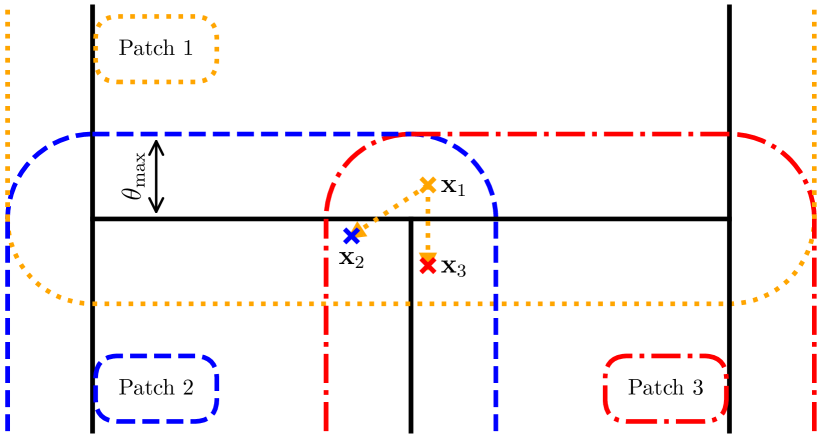
Refer to caption
Figure 10: Counting of galaxy triplets in overlapping (extended) patches. We consider a mock footprint that is split in three patches, which are extended by some scale θmaxsubscript𝜃max\theta_{\mathrm{max}} over their boundary. We also show three galaxies that each lie in a different patch but are contained in the intersection of the three extended patches. When computing the 3PCF multipoles in the first patch, the form of Eq. (B) only allows us to compute the Gnsubscript𝐺𝑛G_{n}s at position 𝐱1subscript𝐱1\mathbf{x}_{1}, meaning that only the depicted triangle is included in the 3PCF. When encountering the same three galaxies in the two other patches, a different reference will be chosen, such that each particular triangle configuration will be six-fold counted across the full footprint.

While the discussion in the main text did solely focus on the efficient estimation of the shear 3PCF on a flat geometry, an actual survey will observe galaxies on the sky and will construct its ellipticity catalog \mathcal{F} based on a spherical topology. However, by cutting out small patches of the curved-sky catalog we can use the flat-sky approximation and apply the methods introduced in Sect. 3 to compute the shear 3PCF for each patch and then average over the individual measurements to obtain an estimate for the shear 3PCF of the full data set.

In a more algorithmic fashion, for mapping a catalog on the sphere to its flat-sky analog 𝒜𝒜\mathcal{A}, one can proceed according to the following steps:

  1. 1.

    Define a domain decomposition of the curved-sky catalog \mathcal{F} into Npsubscript𝑁pN_{\mathrm{p}} smaller patches181818In order to minimize the curved-sky effects we construct the individual patches to have a rectangular shape with each side having a length of 10absentsuperscript10\leq 10^{\circ}.

  2. 2.

    Rotate each patch to the equator. In order to account for the different reference directions of the shapes we make use of the angle_ref method of the healpy.Rotator class.

  3. 3.

    Map each rotated patch onto the flat sky using a sinusoidal projection; call these patches 𝒜i:iI{1,,Np}:subscript𝒜𝑖𝑖𝐼1subscript𝑁p\mathcal{A}_{i}\ :\ i\in I\equiv\{1,\cdots,N_{\mathrm{p}}\}

  4. 4.

    Define the union of the rotated and projected patches in step 3 as the flat-sky analog of the original catalog:
    𝒜iI𝒜isimilar-to𝒜subscript𝑖𝐼subscript𝒜𝑖\mathcal{F}\sim\mathcal{A}\equiv\bigcup_{i\in I}\mathcal{A}_{i}

We are now in a position to use the methods developed in Sect. 3 to measure the correlators on the full survey footprint Υμ×𝒜superscriptsubscriptsuperscriptΥ𝜇𝒜{}^{\mathcal{A}}\Upsilon^{\times}_{\mu} up until some largest separation θmaxsubscript𝜃max\theta_{\mathrm{max}}. For this we combine the multipole components Υμ,n×𝒜isuperscriptsubscriptsuperscriptΥ𝜇𝑛subscript𝒜𝑖{}^{\mathcal{A}_{i}}\Upsilon^{\times}_{\mu,n} in the individual patches 𝒜isubscript𝒜𝑖\mathcal{A}_{i} as follows:

Υ0,n×𝒜(Θ1,Θ2)superscriptsuperscriptsubscriptΥ0𝑛𝒜subscriptΘ1subscriptΘ2\displaystyle{}^{\mathcal{A}}\Upsilon_{0,n}^{\times}(\Theta_{1},\Theta_{2})
i=1Ngalwiγc,iGn3disc(𝜽i;Θ1)Gn3disc(𝜽i;Θ2)absentsuperscriptsubscript𝑖1subscript𝑁galsubscript𝑤𝑖subscript𝛾c𝑖superscriptsubscript𝐺𝑛3discsubscript𝜽𝑖subscriptΘ1superscriptsubscript𝐺𝑛3discsubscript𝜽𝑖subscriptΘ2\displaystyle\equiv\sum_{i=1}^{N_{\mathrm{gal}}}w_{i}\gamma_{\mathrm{c}{,i}}\ G_{n-3}^{\mathrm{disc}}(\boldsymbol{\theta}_{i};\Theta_{1})\ G_{-n-3}^{\mathrm{disc}}(\boldsymbol{\theta}_{i};\Theta_{2})
=p=1Npi=1Ngal,pwiγc,iGn3disc(𝜽i;Θ1)Gn3disc(𝜽i;Θ2)absentsuperscriptsubscript𝑝1subscript𝑁psuperscriptsubscript𝑖1subscript𝑁gal𝑝subscript𝑤𝑖subscript𝛾c𝑖superscriptsubscript𝐺𝑛3discsubscript𝜽𝑖subscriptΘ1superscriptsubscript𝐺𝑛3discsubscript𝜽𝑖subscriptΘ2\displaystyle=\sum_{p=1}^{N_{\mathrm{p}}}\sum_{i=1}^{N_{\mathrm{gal},p}}w_{i}\gamma_{\mathrm{c}{,i}}\ G_{n-3}^{\mathrm{disc}}(\boldsymbol{\theta}_{i};\Theta_{1})\ G_{-n-3}^{\mathrm{disc}}(\boldsymbol{\theta}_{i};\Theta_{2})
p=1NpΥμ,n×𝒜p(Θ1,Θ2).absentsuperscriptsubscript𝑝1subscript𝑁psuperscriptsuperscriptsubscriptΥ𝜇𝑛subscript𝒜𝑝subscriptΘ1subscriptΘ2\displaystyle\equiv\sum_{p=1}^{N_{\mathrm{p}}}{}^{\mathcal{A}_{p}}\Upsilon_{\mu,n}^{\times}(\Theta_{1},\Theta_{2})\ . (61)

We note that in the second step, the inner sum only runs over the Ngal,psubscript𝑁gal𝑝N_{\mathrm{gal},p} galaxies contained in the 𝒜psubscript𝒜𝑝\mathcal{A}_{p}, but the Gndiscsuperscriptsubscript𝐺𝑛discG_{n}^{\mathrm{disc}} are able to access data from 𝒜𝒜\mathcal{A} - this implicit overlap of patches is necessary to account for triplets split between different patches. For implementing the overlap in practice, all that needs to be done is to extend the patches to also include galaxies being separated by at most θmaxsubscript𝜃max\theta_{\mathrm{max}} from the interior of each original patch, but to only consider galaxies within the original patch when evaluating the inner sum in Eq. (B); see Fig. 10 for an illustration.

Appendix C Transformation between shear 3PCF and third-order aperture measures

In this appendix we collect the main equations that are necessary for converting a the shear 3PCF to third-order aperture measures.

C.1 Filter functions

An explicit form for the filter functions F0subscript𝐹0F_{0} and F1subscript𝐹1F_{1} has been derived in SKL05. Here we add the equations for F2subscript𝐹2F_{2} and F3subscript𝐹3F_{3} and adapt all equations to our triangle convention. We begin by defining the helper quantities

Θ2superscriptΘ2\displaystyle\Theta^{2} =θ12θ22+θ12θ32+θ22θ323,absentsuperscriptsubscript𝜃12superscriptsubscript𝜃22superscriptsubscript𝜃12superscriptsubscript𝜃32superscriptsubscript𝜃22superscriptsubscript𝜃323\displaystyle=\sqrt{\frac{\theta_{1}^{2}\theta_{2}^{2}+\theta_{1}^{2}\theta_{3}^{2}+\theta_{2}^{2}\theta_{3}^{2}}{3}}\ , (62)
S𝑆\displaystyle S =θ12θ22θ32Θ6,absentsuperscriptsubscript𝜃12superscriptsubscript𝜃22superscriptsubscript𝜃32superscriptΘ6\displaystyle=\frac{\theta_{1}^{2}\,\theta_{2}^{2}\,\theta_{3}^{2}}{\Theta^{6}}\ , (63)
M𝑀\displaystyle M =Sϑ1ϑ22πΘ4,absent𝑆subscriptitalic-ϑ1subscriptitalic-ϑ22𝜋superscriptΘ4\displaystyle=S\ \frac{\vartheta_{1}\ \vartheta_{2}}{2\pi\,\Theta^{4}}\ , (64)
Z𝑍\displaystyle Z =i=13(θi2+2θi+12+2θi+22)|q𝐢˘|26Θ4,absentsuperscriptsubscript𝑖13superscriptsubscript𝜃𝑖22superscriptsubscript𝜃𝑖122superscriptsubscript𝜃𝑖22superscript˘subscriptq𝐢26superscriptΘ4\displaystyle=\frac{\sum_{i=1}^{3}(-\theta_{i}^{2}+2\theta_{i+1}^{2}+2\theta_{i+2}^{2})|\mathbf{\breve{\mathrm{\textbf{{q}}}_{i}}}|^{2}}{6\Theta^{4}}\ , (65)
fisubscript𝑓𝑖\displaystyle f_{i} =θi+12+θi+222Θ2+q˘i(q˘i+1q˘i+2)|q˘i|2θi+12θi+226Θ2,absentsuperscriptsubscript𝜃𝑖12superscriptsubscript𝜃𝑖222superscriptΘ2superscriptsubscript˘q𝑖subscript˘q𝑖1subscript˘q𝑖2superscriptsubscript˘q𝑖2superscriptsubscript𝜃𝑖12superscriptsubscript𝜃𝑖226superscriptΘ2\displaystyle=\frac{\theta_{i+1}^{2}+\theta_{i+2}^{2}}{2\Theta^{2}}+\frac{\breve{\mathrm{\textbf{{q}}}}_{i}^{*}\left(\breve{\mathrm{\textbf{{q}}}}_{i+1}-\breve{\mathrm{\textbf{{q}}}}_{i+2}\right)}{|\breve{\mathrm{\textbf{{q}}}}_{i}|^{2}}\ \frac{\theta_{i+1}^{2}-\theta_{i+2}^{2}}{6\Theta^{2}}\ , (66)
gisubscript𝑔𝑖\displaystyle g_{i} =θi+12θi+22Θ4+q˘i(q˘i+1q˘i+2)|q˘i|2θi2(θi+22θi+12)3Θ4,absentsuperscriptsubscript𝜃𝑖12superscriptsubscript𝜃𝑖22superscriptΘ4superscriptsubscript˘q𝑖subscript˘q𝑖1subscript˘q𝑖2superscriptsubscript˘q𝑖2superscriptsubscript𝜃𝑖2superscriptsubscript𝜃𝑖22superscriptsubscript𝜃𝑖123superscriptΘ4\displaystyle=\frac{\theta_{i+1}^{2}\,\theta_{i+2}^{2}}{\Theta^{4}}+\frac{\breve{\mathrm{\textbf{{q}}}}_{i}^{*}\left(\breve{\mathrm{\textbf{{q}}}}_{i+1}-\breve{\mathrm{\textbf{{q}}}}_{i+2}\right)}{|\breve{\mathrm{\textbf{{q}}}}_{i}|^{2}}\ \frac{\theta_{i}^{2}\left(\theta_{i+2}^{2}-\theta_{i+1}^{2}\right)}{3\Theta^{4}}\ , (67)

where i{1,2,3}𝑖123i\in\{1,2,3\} and all indices should be taken mod 3mod3\mathrm{mod}\,3. We then have for the filter functions Fμsubscript𝐹𝜇F_{\mu}:

F0(ϑ1,\displaystyle F_{0}(\vartheta_{1}, ϑ2,ϕ;θ1,θ2,θ3)\displaystyle\vartheta_{2},\phi;\theta_{1},\theta_{2},\theta_{3})
=M24|q˘1|2|q˘2|2|q˘3|2Θ6f1 2f2 2f3 2eZ,absent𝑀24superscriptsubscript˘q12superscriptsubscript˘q22superscriptsubscript˘q32superscriptΘ6superscriptsubscript𝑓1absent2superscriptsubscript𝑓2absent2superscriptsubscript𝑓3absent2superscripte𝑍\displaystyle=\frac{M}{24}\ \frac{|\breve{\mathrm{\textbf{{q}}}}_{1}|^{2}|\breve{\mathrm{\textbf{{q}}}}_{2}|^{2}|\breve{\mathrm{\textbf{{q}}}}_{3}|^{2}}{\Theta^{6}}\,f_{1}^{*\,2}f_{2}^{*\,2}f_{3}^{*\,2}\ \mathrm{e}^{-Z}\ , (68)
F1(ϑ1,\displaystyle F_{1}(\vartheta_{1}, ϑ2,ϕ;θ1,θ2,θ3)\displaystyle\vartheta_{2},\phi;\theta_{1},\theta_{2},\theta_{3})
=MeZ[|q˘1|2|q˘2|2|q˘3|224Θ6f3 2f1 2f22\displaystyle=M\,\mathrm{e}^{-Z}\left[\frac{|\breve{\mathrm{\textbf{{q}}}}_{1}|^{2}|\breve{\mathrm{\textbf{{q}}}}_{2}|^{2}|\breve{\mathrm{\textbf{{q}}}}_{3}|^{2}}{24\Theta^{6}}f_{3}^{*\,2}f_{1}^{*\,2}f_{2}^{2}\right.
19q˘3q˘1q˘2 2Θ4f3f1f2g219subscript˘q3subscript˘q1superscriptsubscript˘q2absent2superscriptΘ4superscriptsubscript𝑓3superscriptsubscript𝑓1subscript𝑓2superscriptsubscript𝑔2\displaystyle\hskip 34.14322pt-\frac{1}{9}\frac{\breve{\mathrm{\textbf{{q}}}}_{3}\breve{\mathrm{\textbf{{q}}}}_{1}\breve{\mathrm{\textbf{{q}}}}_{2}^{*\,2}}{\Theta^{4}}f_{3}^{*}f_{1}^{*}f_{2}\,g_{2}^{*}
+127(q˘32q˘12q˘2 4|q˘1|2|q˘2|2|q˘3|2Θ2g2 2\displaystyle\hskip 34.14322pt+\frac{1}{27}\left(\frac{\breve{\mathrm{\textbf{{q}}}}_{3}^{2}\breve{\mathrm{\textbf{{q}}}}_{1}^{2}\breve{\mathrm{\textbf{{q}}}}_{2}^{*\,4}}{|\breve{\mathrm{\textbf{{q}}}}_{1}|^{2}|\breve{\mathrm{\textbf{{q}}}}_{2}|^{2}|\breve{\mathrm{\textbf{{q}}}}_{3}|^{2}\,\Theta^{2}}\,g_{2}^{*\,2}\right.
+2θ32θ12Θ4q˘3q˘1q˘2 2|q˘2|2Θ2f3f1)],\displaystyle\hskip 56.9055pt\left.\left.+\frac{2\theta_{3}^{2}\theta_{1}^{2}}{\Theta^{4}}\ \frac{\breve{\mathrm{\textbf{{q}}}}_{3}\breve{\mathrm{\textbf{{q}}}}_{1}\breve{\mathrm{\textbf{{q}}}}_{2}^{*\,2}}{|\breve{\mathrm{\textbf{{q}}}}_{2}|^{2}\Theta^{2}}\,f_{3}^{*}f_{1}^{*}\right)\right]\ , (69)

where the q˘isubscript˘q𝑖\breve{\mathrm{\textbf{{q}}}}_{i} are given in (11). The other two components follow by cyclically permuting the indices in F1subscript𝐹1F_{1}, i.e. F2=F1(231)subscript𝐹2superscriptsubscript𝐹1231F_{2}=F_{1}^{(231)} and F3=F1(312)subscript𝐹3superscriptsubscript𝐹1312F_{3}=F_{1}^{(312)}. When comparing to the expressions in SKL05, their Fisubscript𝐹𝑖F_{i} is our Fi+2subscript𝐹𝑖2F_{i+2}.

C.2 Transformation to the aperture measures

By evaluating the expressions 3expectation-valuesuperscript3\expectationvalue{\mathcal{M}^{3}}, 2expectation-valuesuperscriptsuperscript2\expectationvalue{\mathcal{M}^{*}\mathcal{M}^{2}}, expectation-valuesuperscript\expectationvalue{\mathcal{M}\mathcal{M}^{*}\mathcal{M}} and 2expectation-valuesuperscript2superscript\expectationvalue{\mathcal{M}^{2}\mathcal{M}^{*}} of the complex aperture measures in terms of the (cross) aperture mass via =ap+i×expectation-valueexpectation-valuesubscriptapiexpectation-valuesubscript\expectationvalue{\mathcal{M}}=\expectationvalue{\mathcal{M}_{\mathrm{ap}}}+\mathrm{i}\expectationvalue{\mathcal{M}_{\times}} one can invert the corresponding linear system to obtain the transformation equations

ap3(θ1,θ2,θ3)delimited-⟨⟩superscriptsubscriptap3subscript𝜃1subscript𝜃2subscript𝜃3\displaystyle\left\langle\mathcal{M}_{\mathrm{ap}}^{3}\right\rangle(\theta_{1},\theta_{2},\theta_{3})
=Re[2(θ1,θ2,θ3)+(θ1,θ2,θ3)\displaystyle\quad\quad=\real\Large[\expectationvalue{\mathcal{M}^{2}\mathcal{M}^{*}}(\theta_{1},\theta_{2},\theta_{3})+\expectationvalue{\mathcal{M}\mathcal{M}^{*}\mathcal{M}}(\theta_{1},\theta_{2},\theta_{3})
+2(θ1,θ2,θ3)+3(θ1,θ2,θ3)]/4,\displaystyle\quad\quad\quad+\expectationvalue{\mathcal{M}^{*}\mathcal{M}^{2}}(\theta_{1},\theta_{2},\theta_{3})+\expectationvalue{\mathcal{M}^{3}}(\theta_{1},\theta_{2},\theta_{3})\Large]/4\ , (70)
×ap2(θ1,θ2,θ3)delimited-⟨⟩subscriptsuperscriptsubscriptap2subscript𝜃1subscript𝜃2subscript𝜃3\displaystyle\left\langle\mathcal{M}_{\times}\mathcal{M}_{\mathrm{ap}}^{2}\right\rangle(\theta_{1},\theta_{2},\theta_{3})
=Im[2(θ1,θ2,θ3)+(θ1,θ2,θ3)\displaystyle\quad=\imaginary\Large[\expectationvalue{\mathcal{M}^{2}\mathcal{M}^{*}}(\theta_{1},\theta_{2},\theta_{3})+\expectationvalue{\mathcal{M}\mathcal{M}^{*}\mathcal{M}}(\theta_{1},\theta_{2},\theta_{3})
2(θ1,θ2,θ3)+3(θ1,θ2,θ3)]/4,\displaystyle\quad\quad-\expectationvalue{\mathcal{M}^{*}\mathcal{M}^{2}}(\theta_{1},\theta_{2},\theta_{3})+\expectationvalue{\mathcal{M}^{3}}(\theta_{1},\theta_{2},\theta_{3})\Large]/4\ , (71)
ap×ap(θ1,θ2,θ3)delimited-⟨⟩subscriptapsubscriptsubscriptapsubscript𝜃1subscript𝜃2subscript𝜃3\displaystyle\left\langle\mathcal{M}_{\mathrm{ap}}\mathcal{M}_{\times}\mathcal{M}_{\mathrm{ap}}\right\rangle(\theta_{1},\theta_{2},\theta_{3})
=Im[2(θ1,θ2,θ3)(θ1,θ2,θ3)\displaystyle\quad=\imaginary\Large[\expectationvalue{\mathcal{M}^{2}\mathcal{M}^{*}}(\theta_{1},\theta_{2},\theta_{3})-\expectationvalue{\mathcal{M}\mathcal{M}^{*}\mathcal{M}}(\theta_{1},\theta_{2},\theta_{3})
+2(θ1,θ2,θ3)+3(θ1,θ2,θ3)]/4,\displaystyle\quad\quad+\expectationvalue{\mathcal{M}^{*}\mathcal{M}^{2}}(\theta_{1},\theta_{2},\theta_{3})+\expectationvalue{\mathcal{M}^{3}}(\theta_{1},\theta_{2},\theta_{3})\Large]/4\ , (72)
ap2×(θ1,θ2,θ3)delimited-⟨⟩superscriptsubscriptap2subscriptsubscript𝜃1subscript𝜃2subscript𝜃3\displaystyle\left\langle\mathcal{M}_{\mathrm{ap}}^{2}\mathcal{M}_{\times}\right\rangle(\theta_{1},\theta_{2},\theta_{3})
=Im[2(θ1,θ2,θ3)+(θ1,θ2,θ3)\displaystyle\quad=\imaginary\Large[-\expectationvalue{\mathcal{M}^{2}\mathcal{M}^{*}}(\theta_{1},\theta_{2},\theta_{3})+\expectationvalue{\mathcal{M}\mathcal{M}^{*}\mathcal{M}}(\theta_{1},\theta_{2},\theta_{3})
+2(θ1,θ2,θ3)+3(θ1,θ2,θ3)]/4,\displaystyle\quad\quad+\expectationvalue{\mathcal{M}^{*}\mathcal{M}^{2}}(\theta_{1},\theta_{2},\theta_{3})+\expectationvalue{\mathcal{M}^{3}}(\theta_{1},\theta_{2},\theta_{3})\Large]/4\ , (73)
ap×2(θ1,θ2,θ3)delimited-⟨⟩subscriptapsuperscriptsubscript2subscript𝜃1subscript𝜃2subscript𝜃3\displaystyle\left\langle\mathcal{M}_{\mathrm{ap}}\mathcal{M}_{\times}^{2}\right\rangle(\theta_{1},\theta_{2},\theta_{3})
=Re[2(θ1,θ2,θ3)+(θ1,θ2,θ3)\displaystyle\quad=\real\Large[\expectationvalue{\mathcal{M}^{2}\mathcal{M}^{*}}(\theta_{1},\theta_{2},\theta_{3})+\expectationvalue{\mathcal{M}\mathcal{M}^{*}\mathcal{M}}(\theta_{1},\theta_{2},\theta_{3})
2(θ1,θ2,θ3)3(θ1,θ2,θ3)]/4,\displaystyle\quad\quad-\expectationvalue{\mathcal{M}^{*}\mathcal{M}^{2}}(\theta_{1},\theta_{2},\theta_{3})-\expectationvalue{\mathcal{M}^{3}}(\theta_{1},\theta_{2},\theta_{3})\Large]/4\ , (74)
×ap×(θ1,θ2,θ3)delimited-⟨⟩subscriptsubscriptapsubscriptsubscript𝜃1subscript𝜃2subscript𝜃3\displaystyle\left\langle\mathcal{M}_{\times}\mathcal{M}_{\mathrm{ap}}\mathcal{M}_{\times}\right\rangle(\theta_{1},\theta_{2},\theta_{3})
=Re[2(θ1,θ2,θ3)(θ1,θ2,θ3)\displaystyle\quad=\real\Large[\expectationvalue{\mathcal{M}^{2}\mathcal{M}^{*}}(\theta_{1},\theta_{2},\theta_{3})-\expectationvalue{\mathcal{M}\mathcal{M}^{*}\mathcal{M}}(\theta_{1},\theta_{2},\theta_{3})
+2(θ1,θ2,θ3)3(θ1,θ2,θ3)]/4,\displaystyle\quad\quad+\expectationvalue{\mathcal{M}^{*}\mathcal{M}^{2}}(\theta_{1},\theta_{2},\theta_{3})-\expectationvalue{\mathcal{M}^{3}}(\theta_{1},\theta_{2},\theta_{3})\Large]/4\ , (75)
×2ap(θ1,θ2,θ3)delimited-⟨⟩superscriptsubscript2subscriptapsubscript𝜃1subscript𝜃2subscript𝜃3\displaystyle\left\langle\mathcal{M}_{\times}^{2}\mathcal{M}_{\mathrm{ap}}\right\rangle(\theta_{1},\theta_{2},\theta_{3})
=Re[2(θ1,θ2,θ3)+(θ1,θ2,θ3)\displaystyle\quad=\real\Large[-\expectationvalue{\mathcal{M}^{2}\mathcal{M}^{*}}(\theta_{1},\theta_{2},\theta_{3})+\expectationvalue{\mathcal{M}\mathcal{M}^{*}\mathcal{M}}(\theta_{1},\theta_{2},\theta_{3})
+2(θ1,θ2,θ3)3(θ1,θ2,θ3)]/4,\displaystyle\quad\quad+\expectationvalue{\mathcal{M}^{*}\mathcal{M}^{2}}(\theta_{1},\theta_{2},\theta_{3})-\expectationvalue{\mathcal{M}^{3}}(\theta_{1},\theta_{2},\theta_{3})\Large]/4\ , (76)
×3(θ1,θ2,θ3)delimited-⟨⟩superscriptsubscript3subscript𝜃1subscript𝜃2subscript𝜃3\displaystyle\left\langle\mathcal{M}_{\times}^{3}\right\rangle(\theta_{1},\theta_{2},\theta_{3})
=Im[2(θ1,θ2,θ3)+(θ1,θ2,θ3)\displaystyle\quad=\imaginary\Large[\expectationvalue{\mathcal{M}^{2}\mathcal{M}^{*}}(\theta_{1},\theta_{2},\theta_{3})+\expectationvalue{\mathcal{M}\mathcal{M}^{*}\mathcal{M}}(\theta_{1},\theta_{2},\theta_{3})
+2(θ1,θ2,θ3)3(θ1,θ2,θ3)]/4.\displaystyle\quad\quad+\expectationvalue{\mathcal{M}^{*}\mathcal{M}^{2}}(\theta_{1},\theta_{2},\theta_{3})-\expectationvalue{\mathcal{M}^{3}}(\theta_{1},\theta_{2},\theta_{3})\Large]/4\ . (77)

In the main text we average over the three permutations of the correlators where both, apsubscriptap\mathcal{M}_{\mathrm{ap}} and ×subscript\mathcal{M}_{\times} are present. This implies that the covariance of those components is smaller than the covariance of ×3delimited-⟨⟩superscriptsubscript3\left\langle\mathcal{M}_{\times}^{3}\right\rangle.

For a tomographic setup we need to make the adjustment that each correlator also depends on the redshift bins, i.e. we have

ap3(θ1,θ2,θ3)ap3(θ1,θ2,θ3;Z1,Z2,Z3).delimited-⟨⟩superscriptsubscriptap3subscript𝜃1subscript𝜃2subscript𝜃3delimited-⟨⟩superscriptsubscriptap3subscript𝜃1subscript𝜃2subscript𝜃3subscript𝑍1subscript𝑍2subscript𝑍3\displaystyle\left\langle\mathcal{M}_{\mathrm{ap}}^{3}\right\rangle(\theta_{1},\theta_{2},\theta_{3})\rightarrow\left\langle\mathcal{M}_{\mathrm{ap}}^{3}\right\rangle(\theta_{1},\theta_{2},\theta_{3};Z_{1},Z_{2},Z_{3})\ . (78)

We note that due to the symmetries of the form

ap3(\displaystyle\left\langle\mathcal{M}_{\mathrm{ap}}^{3}\right\rangle( θ1,θ2,θ3;Z1,Z2,Z3)\displaystyle\theta_{1},\theta_{2},\theta_{3};Z_{1},Z_{2},Z_{3})
=ap3(θ1,θ2,θ3;Zπ(1),Zπ(2),Zπ(3)),absentdelimited-⟨⟩superscriptsubscriptap3subscript𝜃1subscript𝜃2subscript𝜃3subscript𝑍𝜋1subscript𝑍𝜋2subscript𝑍𝜋3\displaystyle=\left\langle\mathcal{M}_{\mathrm{ap}}^{3}\right\rangle(\theta_{1},\theta_{2},\theta_{3};Z_{\pi(1)},Z_{\pi(2)},Z_{\pi(3)})\ , (79)
×2ap(\displaystyle\left\langle\mathcal{M}_{\times}^{2}\mathcal{M}_{\mathrm{ap}}\right\rangle( θ1,θ2,θ3;Z1,Z2,Z3)\displaystyle\theta_{1},\theta_{2},\theta_{3};Z_{1},Z_{2},Z_{3})
=ap×2(θ3,θ1,θ2;Z1,Z2,Z3),absentdelimited-⟨⟩subscriptapsuperscriptsubscript2subscript𝜃3subscript𝜃1subscript𝜃2subscript𝑍1subscript𝑍2subscript𝑍3\displaystyle=\left\langle\mathcal{M}_{\mathrm{ap}}\mathcal{M}_{\times}^{2}\right\rangle(\theta_{3},\theta_{1},\theta_{2};Z_{1},Z_{2},Z_{3})\ , (80)

for any πS3𝜋subscript𝑆3\pi\in S_{3}, the transformation equations can be reduced to the shorter expressions found i.e. in SKL05:

ap3(θ1,θ2,θ3)delimited-⟨⟩superscriptsubscriptap3subscript𝜃1subscript𝜃2subscript𝜃3\displaystyle\left\langle\mathcal{M}_{\mathrm{ap}}^{3}\right\rangle(\theta_{1},\theta_{2},\theta_{3})
=Re[2(θ1,θ2,θ3)+2(θ1,θ3,θ2)\displaystyle\quad=\real\Large[\expectationvalue{\mathcal{M}^{*}\mathcal{M}^{2}}(\theta_{1},\theta_{2},\theta_{3})+\expectationvalue{\mathcal{M}^{*}\mathcal{M}^{2}}(\theta_{1},\theta_{3},\theta_{2})
+2(θ2,θ3,θ1)+3(θ1,θ2,θ3)]/4,\displaystyle\quad\quad+\expectationvalue{\mathcal{M}^{*}\mathcal{M}^{2}}(\theta_{2},\theta_{3},\theta_{1})+\expectationvalue{\mathcal{M}^{3}}(\theta_{1},\theta_{2},\theta_{3})\Large]/4\ , (81)
ap2×(θ1,θ2,θ3)delimited-⟨⟩superscriptsubscriptap2subscriptsubscript𝜃1subscript𝜃2subscript𝜃3\displaystyle\left\langle\mathcal{M}_{\mathrm{ap}}^{2}\mathcal{M}_{\times}\right\rangle(\theta_{1},\theta_{2},\theta_{3})
=Im[2(θ1,θ2,θ3)+2(θ1,θ3,θ2)\displaystyle\quad=\imaginary\Large[-\expectationvalue{\mathcal{M}^{*}\mathcal{M}^{2}}(\theta_{1},\theta_{2},\theta_{3})+\expectationvalue{\mathcal{M}^{*}\mathcal{M}^{2}}(\theta_{1},\theta_{3},\theta_{2})
+2(θ2,θ3,θ1)+3(θ1,θ2,θ3)]/4,\displaystyle\quad\quad+\expectationvalue{\mathcal{M}^{*}\mathcal{M}^{2}}(\theta_{2},\theta_{3},\theta_{1})+\expectationvalue{\mathcal{M}^{3}}(\theta_{1},\theta_{2},\theta_{3})\Large]/4\ , (82)
ap×2(θ1,θ2,θ3)delimited-⟨⟩subscriptapsuperscriptsubscript2subscript𝜃1subscript𝜃2subscript𝜃3\displaystyle\left\langle\mathcal{M}_{\mathrm{ap}}\mathcal{M}_{\times}^{2}\right\rangle(\theta_{1},\theta_{2},\theta_{3})
=Re[2(θ1,θ2,θ3)+2(θ1,θ3,θ2)\displaystyle\quad=\real\Large[\expectationvalue{\mathcal{M}^{*}\mathcal{M}^{2}}(\theta_{1},\theta_{2},\theta_{3})+\expectationvalue{\mathcal{M}^{*}\mathcal{M}^{2}}(\theta_{1},\theta_{3},\theta_{2})
2(θ2,θ3,θ1)3(θ1,θ2,θ3)]/4,\displaystyle\quad\quad-\expectationvalue{\mathcal{M}^{*}\mathcal{M}^{2}}(\theta_{2},\theta_{3},\theta_{1})-\expectationvalue{\mathcal{M}^{3}}(\theta_{1},\theta_{2},\theta_{3})\Large]/4\ , (83)
×3(θ1,θ2,θ3)delimited-⟨⟩superscriptsubscript3subscript𝜃1subscript𝜃2subscript𝜃3\displaystyle\left\langle\mathcal{M}_{\times}^{3}\right\rangle(\theta_{1},\theta_{2},\theta_{3})
=Im[2(θ1,θ2,θ3)+2(θ1,θ3,θ2)\displaystyle\quad=\imaginary\Large[\expectationvalue{\mathcal{M}^{*}\mathcal{M}^{2}}(\theta_{1},\theta_{2},\theta_{3})+\expectationvalue{\mathcal{M}^{*}\mathcal{M}^{2}}(\theta_{1},\theta_{3},\theta_{2})
+2(θ2,θ3,θ1)3(θ1,θ2,θ3)]/4,\displaystyle\quad\quad+\expectationvalue{\mathcal{M}^{*}\mathcal{M}^{2}}(\theta_{2},\theta_{3},\theta_{1})-\expectationvalue{\mathcal{M}^{3}}(\theta_{1},\theta_{2},\theta_{3})\Large]/4\ , (84)

where we suppressed the redshift bin indices for better readability.

We note that if one is solely interested in the values of ap3delimited-⟨⟩superscriptsubscriptap3\left\langle\mathcal{M}_{\mathrm{ap}}^{3}\right\rangle and ×3delimited-⟨⟩superscriptsubscript3\left\langle\mathcal{M}_{\times}^{3}\right\rangle, as well as in the averaged quantities

ap×2av.superscriptdelimited-⟨⟩subscriptapsuperscriptsubscript2av\displaystyle\left\langle\mathcal{M}_{\mathrm{ap}}\mathcal{M}_{\times}^{2}\right\rangle^{\mathrm{av.}} (×2ap+×ap×+ap×2)3,absentdelimited-⟨⟩superscriptsubscript2subscriptapdelimited-⟨⟩subscriptsubscriptapsubscriptdelimited-⟨⟩subscriptapsuperscriptsubscript23\displaystyle\equiv\frac{\left(\left\langle\mathcal{M}_{\times}^{2}\mathcal{M}_{\mathrm{ap}}\right\rangle+\left\langle\mathcal{M}_{\times}\mathcal{M}_{\mathrm{ap}}\mathcal{M}_{\times}\right\rangle+\left\langle\mathcal{M}_{\mathrm{ap}}\mathcal{M}_{\times}^{2}\right\rangle\right)}{3}\ , (85)
ap2×av.superscriptdelimited-⟨⟩superscriptsubscriptap2subscriptav\displaystyle\left\langle\mathcal{M}_{\mathrm{ap}}^{2}\mathcal{M}_{\times}\right\rangle^{\mathrm{av.}} (ap2×+ap×ap+×ap2)3,absentdelimited-⟨⟩superscriptsubscriptap2subscriptdelimited-⟨⟩subscriptapsubscriptsubscriptapdelimited-⟨⟩subscriptsuperscriptsubscriptap23\displaystyle\equiv\frac{\left(\left\langle\mathcal{M}_{\mathrm{ap}}^{2}\mathcal{M}_{\times}\right\rangle+\left\langle\mathcal{M}_{\mathrm{ap}}\mathcal{M}_{\times}\mathcal{M}_{\mathrm{ap}}\right\rangle+\left\langle\mathcal{M}_{\times}\mathcal{M}_{\mathrm{ap}}^{2}\right\rangle\right)}{3}\ , (86)

it is sufficient to only compute the 3PCF for Z1Z2Z3subscript𝑍1subscript𝑍2subscript𝑍3Z_{1}\leq Z_{2}\leq Z_{3}, if one uses the full transformation equations (C.2-77) and additionally symmetrizes them over the three aperture radii.

Appendix D Measurements in the T17 Ensemble

Fig. 11 displays the measurement of the third-order aperture statistics in the T17 ensemble consisting of 194419441944 mock ellipticity catalogs mimicking the KiDS-1000 survey. We see that most of the cosmological signal is contained in tomographic bin combinations consisting of high–z𝑧z bins. However, for a cosmological analysis, one should also include the low–z𝑧z bins, as those will help constraining parameters related to the intrinsic alignment model. We also see that none of the three cross-aperture measures yields a significant signal, showing that neither such spurious signal is present in the mock ellipticity catalogs nor that it is created by our estimation procedure. Finally, we compare our measurement to the theoretical prediction, for which we are using the model introduced in Heydenreich et al. (2023). On small angular scales, we see that the measurement does slightly over-predict the theory, which we attribute to the reduced-shear effect that are included in the T17 ensemble, but not in the theory. On large angular scales, however, the measurement does slightly underpredict the theoretical prediction. One reason for this could lie in the lens-shell thickness in the T17 ensemble; in particular Takahashi et al. (2017) show that on the level of the shear 2PCF this effect can cause a suppression of the signal of up to 10%percent1010\% for angular separations of about 100superscript100100^{\prime}. Besides these two effects, a part of the discrepancy between the theory and the measurement could also lie in the limited accuracy of the Bihalofit model (Takahashi et al. 2020), which is at the 10%percent1010\%-level.

Refer to caption
Figure 11: Tomographic third-order aperture mass statistics in the T17 ensemble. In each panel, we show the measured statistic for one configuration of the tomographic bins. The mean ap3superscriptsubscriptap3\mathcal{M}_{\mathrm{ap}}^{3} signal and its standard deviation are plotted as the blue solid line and the blue error band. The other solid lines indicate the absolute values of the remaining third-order measures and the 1σ1𝜎1\sigma uncertainty level of those measures are indicated by the grey dashed (dotted) lines. The theoretical prediction is shown as the black dotted line.

Appendix E Accuracy requirements

Refer to caption
Figure 12: Mean signal and detectability of the higher-order multipoles Υ0,n×superscriptsubscriptΥ0𝑛\Upsilon_{0,n}^{\times} in the SLICS ensemble, after averaging over all 819 realizations. In the top row, we show the mean signal from the noiseless SLICS ensemble. To aid the visualization we normalize the multipoles by the product of the corresponding angular bins and further use a logarithmic scaling for positive and negative values in the colormap. In the second row, we show the signal-to-noise ratio of the modulus of the corresponding multipole component. The third and fourth rows display the same measurements when shape noise is included in the mocks.

E.1 Three Point Correlation Function

In Fig. 12 we show the detection significance of some multipoles Υ0,n×superscriptsubscriptΥ0𝑛\Upsilon_{0,n}^{\times} in the SLICS ensemble for noisy and noiseless data. We see that most of the signal contribution stems from the lowest-order multipoles. This is expected as the shear 3PCF does not contain high-frequency oscillations in the φ𝜑\varphi direction. We also see that shape noise strongly depletes the detection significance of the individual elements; we note that for a stage-IV survey having a significantly higher source density this effect will not be as severe. The plots for the three remaining Υμ,n×superscriptsubscriptΥ𝜇𝑛\Upsilon_{\mu,n}^{\times} all follow the same trend.

E.2 Third-order aperture mass

With the third-order aperture mass being an integrated measure of the shear 3PCF for which the time and space complexity are strongly dependent on the number of radial bins and the largest considered multipole, one should investigate the convergence of the numerical integration for various binning choices. In Fig. 13 we fix the largest multipole nmax=20subscript𝑛max20n_{\mathrm{max}}=20 and compare the numerical integration of the 3PCF for a range of logarithmic bin widths b𝑏b. For the equal-scale apertures, we find that choosing a value of b1.1𝑏1.1b\approx 1.1 yields per-cent level accuracy. This value is similar to the corresponding value found by previous studies (Fu et al. 2014; Secco et al. 2022) examining the convergence of the numerical integration using TreeCorr. We further show in Fig. 13 that our choice of b1.15𝑏1.15b\approx 1.15 for the computation of the numerical covariance from the T17 ensemble yields sufficiently accurate data vectors for aperture scales of more than 4superscript44^{\prime}.191919We note that as the ellipticity data in the T17 ensemble itself is pixelized on a grid with a sidelength of  0.4absentsuperscript0.4\approx\,0.4^{\prime}, the measurements of ap3delimited-⟨⟩superscriptsubscriptap3\left\langle\mathcal{M}_{\mathrm{ap}}^{3}\right\rangle are biased low for small aperture scales, independent of the smallest separation considered in the 3PCF. For the multiscale aperture statistics we find similar convergence properties, except for the cases when two aperture radii are considerably smaller than the third one.

In Fig. 14 we compare how limiting the number of considered multipoles impacts the expected value of ap3delimited-⟨⟩superscriptsubscriptap3\left\langle\mathcal{M}_{\mathrm{ap}}^{3}\right\rangle. We find, as before, a very fast convergence for the equal-scale aperture statistics, while for the general case, there is a strong dependence of the level of convergence on the ratio between the two smallest and the largest aperture radii. This behaviour can be understood as follows: In the case of two small and one large aperture radii the associated ap3delimited-⟨⟩superscriptsubscriptap3\left\langle\mathcal{M}_{\mathrm{ap}}^{3}\right\rangle is dominated by squeezed triangle configurations. As such configurations mainly receive contributions from the multipole components Υμ,n(Θ,Θ)subscriptΥ𝜇𝑛ΘΘ\Upsilon_{\mu,n}(\Theta,\Theta) and those are precisely the ones having a nonvanishing and detectable signal for large multipole orders (see Fig. 12), we do expect a slower convergence.
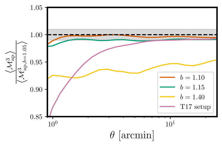
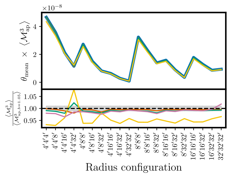
Refer to caption
Refer to caption
Figure 13: Accuracy of the numerical integration of the shear 3PCF to the third-order aperture statistics for different logarithmic spacings of radial bins, as well as for the radial binning that was used for the computation of the covariance in the T17 ensemble. All measurements are done in the SLICS ensemble. In the upper panel, we show the ratio between ap3delimited-⟨⟩superscriptsubscriptap3\left\langle\mathcal{M}_{\mathrm{ap}}^{3}\right\rangle when estimated using some logarithmic bin width b𝑏b for the shear 3PCF and the corresponding result with b1.05𝑏1.05b\equiv 1.05. In the lower panel, we show the corresponding results when allowing for unequal aperture filters.
Refer to caption
Refer to caption
Figure 14: Impact of higher-order multipoles of the shear 3PCF on the third-order aperture statistics in the SLICS ensemble. In the upper panel of the top (bottom) figure, we show the estimated signal for the equal-scale (unequal-scale) statistics, when using only the first nmaxsubscript𝑛maxn_{\mathrm{max}} multipoles. The lower panel displays the decimal logarithm of the fractional difference between the measurement using 505050 multipoles and the measurements using only multipoles up until nmaxsubscript𝑛maxn_{\mathrm{max}}.