Denoising Diffusion Probabilistic Models for Hardware-Impaired Communications

Abstract

Generative AI has received significant attention among a spectrum of diverse industrial and academic domains, thanks to the magnificent results achieved from deep generative models such as generative pre-trained transformers (GPT) and diffusion models. In this paper, we explore the applications of denoising diffusion probabilistic models (DDPMs) in wireless communication systems under practical assumptions such as hardware impairments (HWI), low-SNR regime, and quantization error. Diffusion models are a new class of state-of-the-art generative models that have already showcased notable success with some of the popular examples by OpenAI and Google Brain. The intuition behind DDPM is to decompose the data generation process over small “denoising” steps. Inspired by this, we propose using denoising diffusion model-based receiver for a practical wireless communication scheme, while providing network resilience in low-SNR regimes, non-Gaussian noise, different HWI levels, and quantization error. We evaluate the reconstruction performance of our scheme in terms of mean-squared error (MSE) metric. Our results show that more than $25$ dB improvement in MSE is achieved compared to deep neural network (DNN)-based receivers. We also highlight robust out-of-distribution performance under non-Gaussian noise.

I Introduction

The emergence of innovative approaches in generative artificial intelligence (GenAI) has lead to the development of novel ideas for AI-based systems [1]. At the same time, from data communication and networking perspective, “connected intelligence” is envisioned as the most significant driving force in the sixth generation (6G) of communications—machine learning (ML) and AI algorithms are envisioned to be widely incorporated into 6G networks, realizing “AI-native” wireless systems [3, 2]. This underscores the need for novel AI/ML-based solutions to be tailored for the emerging communication scenarios [4, 5].

Most of the research carried out so far on AI-native wireless has been focused on “discriminative models”. One can consider [6] and [7] as two seminal papers that have attracted remarkable attention in both academia and industry. From a very high-level perspective, the goal of such models is to simply learn the “boundaries” between classes or latent spaces of high-dimensional signals. On the other hand, “generative models” are aimed to learn the “representations” of signals, and generate the desired samples accordingly. In this paper, we take a radically different approach, and our aim is to unleash the power of GenAI for wireless systems.

One of the recent breakthroughs in GenAI is the evolution of diffusion models, as the new state-of-the-art family of generative models [8]. It has lead to unprecedented results in different applications such as computer vision, natural language processing (NLP), and medical imaging [9]. The key idea behind diffusion models is that if we could develop an ML model that can learn the systematic decay of information then it should be possible to “reverse” the process and recover the information back from the noisy/erroneous data. The close underlying relation between the key concepts on how diffusion models work and the problems in wireless communications has motivated us to carry out this research. Notably, the incorporation of diffusion models into wireless communication problems is still in its infancy, hoping that this paper would shed light on some of the possible directions.

Ongoing research on diffusion models encompasses both theoretical advancements and practical applications across different domains of computer science society. However, there have been only a few papers in wireless communications literature that have started looking into the potential merits of diffusion models for wireless systems [5, 13, 10, 11, 12]. The authors in [5] study a workflow for utilizing diffusion models in wireless network management. They exploit the flexibility and exploration ability of diffusion models for generating contracts using diffusion models in mobile AI-generated content services as a use-case. Diffusion models are utilized in [10] to generate synthetic channel realizations. The authors tackle the problem of differentiable channel model within the training process of end-to-end ML-based communications. The results highlight the performance of diffusion models as an alternative to generative adversarial network (GAN)-based schemes. The authors show that GANs experience unstable training and less diversity in generation performance, while diffusion models maintain a more stable training process and a better generalization in inference. Noise-conditioned neural networks are employed in [11] for channel estimation in multi-input-multi-output (MIMO) wireless communications. The authors employ RefineNet neural architecture and run posterior sampling to generate channel estimations based on the pilot signals observed at the receiver. The results in [11] highlight a competitive performance for both in- and out-of-distribution (OOD) scenarios compared to GANs. In [12], deep learning-based joint source-channel coding (Deep-JSCC) is combined with diffusion models to complement digital communication schemes with a generative component. The results indicate that the perceptual quality of reconstruction can be improved by employing diffusion models.

Despite the close relation between the “denoise-and-generate” characteristics of diffusion models and the problems in communication theory, to the best of our knowledge, there is only one preprint [13] in the literature that studies the application of denoising diffusion models in wireless to help improve the receiver’s performance in terms of noise removal. The authors utilize a diffusion model and call it channel denoising diffusion model (CDDM). However, the paper has some drawbacks, which need further considerations. Specifically, i) the authors do not evaluate the performance of their CDDM module under realistic scenarios such as hardware impairments (HWI), low-SNR regimes, and non-Gaussian noise. Rather, their goal is to simply compensate for the channel noise and equalization errors. ii) To reconstruct and generate samples, the authors implement another neural decoder block at the receiver in addition to CDDM. However, having two different ML models, each maintaining a distinct objective function can impose computational overhead to the network. iii) The proposed scheme in [13] relies on the channel state information (CSI) knowledge at the diffusion module, and the transmitter has to feed back the CSI data to the receiver, which can cause communication overhead and might not be aligned with communication standards.

Our Work

In this paper, we study the implementation of denoising diffusion probabilistic models (DDPM), proposed by Ho et al. in 2020 [8], for a practical wireless communication systems with HWIs. The key idea of DDPM is to decompose the data generation process into subsequent “denoising” steps and then gradually generating the desired samples out of noise. Inspired by the recent visions on AI-native wireless for 6G [2], our general idea in this paper is that instead of designing a communication system which avoids HWI and estimation/decoding errors, we can train the network to handle such distortions, aiming to introduce native resilience for wireless AI [2, 3, 4].

In our proposed approach, a DDPM is employed at the receiver side (without relying on any other conventional autoencoder in contrast to [13]) to enhance the resilience of the wireless system against practical non-idealities such as HWI and quantization error. Our DDPM is parameterized by a neural network (NN) comprised of conditional linear layers. Inspired by the Transformer paper (Vaswani et al., 2017 [14]), we only employ one model for the entire denoising time-steps by incorporating the time embeddings into the model. After the diffusion model is trained to generate data samples out of noise, the receiver runs the reverse diffusion process algorithm, starting from the distorted received signals, to reconstruct the transmitted data. We demonstrate the resilience of our DDPM-based approach in different scenarios, including low-SNR regimes, non-Gaussian noise, different HWI levels, and quantization error, which were not addressed in [13]. We also evaluate the mean-squared error (MSE) of our scheme, highlighting more than $25$ dB performance improvement compared to the deep neural network (DNN)-based receiver of [7] as one of the promising benchmark designs in ML-based communications systems.

In the following sections, we first introduce the concept of DDPMs together with the main formulas in Section II. Our system model is introduced in Section III, where we provide the generic formulations and the details of the neural architecture and algorithms. Then, we study numerical evaluations in Section IV, and conclude the paper in Section V.

II Preliminaries on DDPMs

Diffusion models are a new class of generative models that are inspired by non-equilibrium thermodynamics [8]. They consist of two diffusion processes, i.e., the forward and the reverse process. During the forward diffusion steps, random perturbation noise is purposefully added to the original data. Then in a reverse process, DDPMs learn to construct the desired data samples out of noise.

Let ${\bf x}_{0}$ be a data sample from some distribution ${q}({\bf x}_{0})$. For a finite number, $T$, of time-steps, the forward diffusion process $q({\bf x}_{t}|{\bf x}_{t-1})$ is defined by adding Gaussian noise at each time-step $t\in[T]$ according to a known “variance schedule” $0<\beta_{1}<\beta_{2}<\cdots<\beta_{T}<1$. This can be formulated as

$$q(\mathbf{x}_{t}|\mathbf{x}_{t-1}) \sim\mathcal{N}(\mathbf{x}_{t};\sqrt{1-\beta_{t}}\mathbf{x}_{t-1},\beta_{t}\mathbf{I}),$$ (1)

$$q(\mathbf{x}_{1:T}|\mathbf{x}_{0}) =\prod^{T}_{t=1}q(\mathbf{x}_{t}|\mathbf{x}_{t-1}).\vspace{-1mm}$$ (2)

Invoking (2), the data sample gradually loses its distinguishable features as the time-step goes on, where with $T\!\rightarrow\!\infty$, ${\bf x}_{T}$ approaches an isotropic Gaussian distribution with covariance matrix ${\bf\Sigma}\!=\!\sigma^{2}\mathbf{I}$ for some $\sigma\!>\!0$ [8]. According to (1), each new sample at time-step $t$ can be drawn from a conditional Gaussian distribution with mean vector ${\mathbf{\mu}}_{t}=\sqrt{1-\beta_{t}}\mathbf{x}_{t-1}$ and covariance matrix ${\bf\Sigma}^{2}_{t}=\beta_{t}\bf I$. Hence, the forward process is realized by sampling from a Gaussian noise $\bm{\epsilon}_{t-1}\sim{\cal N}(\bf 0,I)$ and setting

$${\bf x}_{t}=\sqrt{1-\beta_{t}} {\bf x}_{t-1}+\sqrt{\beta_{t}}{\bm{\epsilon}}_{t-1}.$$ (3)

A useful property for the forward process in (3) is that we can sample ${\bf{x}}_{t}$ at any arbitrary time step $t$ in a closed-form expression, through recursively applying the reparameterization trick from ML literature [15]. This results in

$$\mathbf{x}_{t} =\sqrt{\bar{\alpha}_{t}}\mathbf{x}_{0}+\sqrt{1-\bar{\alpha}_{t}}\bm{\epsilon}_{0},$$ (4)

$$q({\bf x}_{t}|{\bf x}_{0}) \sim\mathcal{N}\left({\bf x}_{t};\sqrt{\bar{\alpha}_{t}}{\bf x}_{0},(1-\bar{\alpha}_{t})\mathbf{I}\right),$$ (5)

where $\bar{\alpha}_{t}\!=\!\prod_{i=1}^{t}(1-\alpha_{i})$ and $\alpha_{t}=1-\beta_{t}$ [15].

Now the problem is to reverse the process in (4) and sample from $q(\mathbf{x}_{t-1}|\mathbf{x}_{t})$, so that we regenerate the true samples from $\mathbf{x}_{T}$. According to [8], for $\beta_{t}$ small enough, $q(\mathbf{x}_{t-1}|\mathbf{x}_{t})$ also follows Gaussian distribution $\forall t\in[T]$. However, we cannot estimate the distribution, since it requires knowing the distribution of all possible data samples (or equivalently exploiting the entire dataset). Hence, to approximate the conditional probabilities and run the reverse diffusion process, we need to learn a probabilistic model $p_{\bm{\theta}}(\mathbf{x}_{t-1}|\mathbf{x}_{t})$ that is parameterized by ${\bm{\theta}}$. According to the above explanations, the following expressions can be written

$$p_{\bm{\theta}}(\mathbf{x}_{t-1}|\mathbf{x}_{t}) \sim\mathcal{N}(\mathbf{x}_{t-1};\bm{\mu}_{\bm{\theta}}(\mathbf{x}_{t},t),\mathbf{\Sigma}_{\bm{\theta}}(\mathbf{x}_{t},t)),$$ (6)

$$p_{\bm{\theta}}(\mathbf{x}_{0:T}) =p(\mathbf{x}_{T})\prod^{T}_{t=1}p_{\bm{\theta}}(\mathbf{x}_{t-1}|\mathbf{x}_{t}).$$ (7)

Hence, the problem simplifies to learning the mean vector $\bm{\mu}_{\bm{\theta}}(x_{t},t)$ and the covariance matrix $\mathbf{\Sigma}_{\bm{\theta}}(x_{t},t)$ for the probabilistic model $p_{\bm{\theta}}(\cdot)$, where an NN can be trained to approximate (learn) the reverse process.

Before proceeding with the details of learning the reverse diffusion process, we note that if we condition the reverse process on ${\bf x}_{0}$, this conditional probability becomes tractable. The intuition behind this could be explained as follows. A painter (our generative model) requires a reference image ${\bf x}_{0}$ to be able to gradually draw a picture. Hence, when we have ${\bf x}_{0}$ as a reference, we can take a small step backwards from noise to generate the data samples. Then, the reverse step is formulated as $q({\bf x}_{t-1}|{\bf x}_{t},{\bf x}_{0})$. Mathematically speaking, we can derive $q({\bf x}_{t-1}|{\bf x}_{t},{\bf x}_{0})$ using Bayes rule as follows.

$$q(\mathbf{x}_{t-1}|\mathbf{x}_{t},\mathbf{x}_{0}) \sim\mathcal{N}(\mathbf{x}_{t-1};\hskip 4.2679pt{\tilde{\bm{\mu}}}(\mathbf{x}_{t},\mathbf{x}_{0},t),{\tilde{\beta}_{t}}\mathbf{I}),$$ (8)

where

$${\tilde{\bm{\mu}}}(\mathbf{x}_{t},\mathbf{x}_{0},t) =\frac{\sqrt{\alpha_{t}}(1-\bar{\alpha}_{t-1})}{1-\bar{\alpha}_{t}}{\bf x}_{t}+\frac{\sqrt{\bar{\alpha}_{t-1}}\beta_{t}}{1-\bar{\alpha}_{t}}{\bf x}_{0},\text{\hskip 5.69054ptand}$$ (9)

$${\tilde{\beta}_{t}} =\frac{1-\bar{\alpha}_{t-1}}{1-\bar{\alpha}_{t}}\beta_{t}.$$ (10)

Invoking (10), one can infer that the covariance matrix in (8) has no learnable parameter. Hence, we simply need to learn the mean vector ${\tilde{\bm{\mu}}}(\mathbf{x}_{t},\mathbf{x}_{0},t)$. To further simplify (9), we note that thanks to the reparameterization trick and with a similar approach to (4), we can express ${\bf x}_{0}$ as follows.

$$\mathbf{x}_{0}=\frac{1}{\sqrt{\bar{\alpha}_{t}}}(\mathbf{x}_{t}-\sqrt{1-\bar{\alpha}_{t}}\bm{\epsilon}_{t}).$$ (11)

Substituting ${\bf x}_{0}$ in (9) by (11) results in

$$\begin{aligned} \tilde{\bm{\mu}}(\mathbf{x}_{t},\mathbf{x}_{0},t)={\frac{1}{\sqrt{\alpha_{t}}}\Big{(}\mathbf{x}_{t}-\frac{1-\alpha_{t}}{\sqrt{1-\bar{\alpha}_{t}}}\bm{\epsilon}_{t}\Big{)}}.\end{aligned}$$ (12)

Now we can learn the conditioned probability distribution $p_{\bm{\theta}}(\mathbf{x}_{t-1}|\mathbf{x}_{t})$ of the reverse diffusion process by training a NN that approximates $\tilde{\bm{\mu}}(\mathbf{x}_{t},\mathbf{x}_{0},t)$. Therefore, we simply need to set the approximated mean vector $\bm{\mu}_{\bm{\theta}}(\mathbf{x}_{t},t)$ to have the same form as the target mean vector $\tilde{\bm{\mu}}(\mathbf{x}_{t},\mathbf{x}_{0},t)$. Since $\mathbf{x}_{t}$ is known at time-step $t$, we can reparameterize the NN to make it approximate $\bm{\epsilon}_{t}$ from the input $\mathbf{x}_{t}$. Compiling these facts results in the following expression for $\bm{\mu}_{\bm{\theta}}(\mathbf{x}_{t},t)$

$$\bm{\mu}_{\bm{\theta}}(\mathbf{x}_{t},t) ={\frac{1}{\sqrt{\alpha_{t}}}\Big{(}\mathbf{x}_{t}-\frac{1-\alpha_{t}}{\sqrt{1-\bar{\alpha}_{t}}}\bm{\epsilon}_{\bm{\theta}}(\mathbf{x}_{t},t)\Big{)}},$$ (13)

where $\bm{\epsilon}_{\bm{\theta}}(\mathbf{x}_{t},t)$ denotes our NN.

We now define the loss function $\mathcal{L}_{t}$ aiming to minimize the difference between $\bm{\mu}_{\bm{\theta}}(\mathbf{x}_{t},t)$ and $\tilde{\bm{\mu}}(\mathbf{x}_{t},\mathbf{x}_{0},t)$.

$$\mathcal{L}_{t} ={\mathbb{E}}_{\begin{subarray}{l}t\sim{\mathsf{Unif}}[T]\\ {\bf x}_{0}\sim q({\bf x}_{0})\\ \bm{\epsilon}_{0}\sim\mathcal{N}(0,\bf{I})\\ \end{subarray}}\Big{[}\|\bm{\epsilon}_{t}-\bm{\epsilon}_{\bm{\theta}}(\mathbf{x}_{t},t)\|^{2}\Big{]}$$

$$={\mathbb{E}}_{\begin{subarray}{l}t\sim{\mathsf{Unif}}[T]\\ {\bf x}_{0}\sim q({\bf x}_{0})\\ \bm{\epsilon}_{0}\sim\mathcal{N}(0,\bf{I})\\ \end{subarray}}\Big{[}\|\bm{\epsilon}_{t}-\bm{\epsilon}_{\bm{\theta}}(\sqrt{\bar{\alpha}_{t}}\mathbf{x}_{0}+\sqrt{1-\bar{\alpha}_{t}}\bm{\epsilon}_{t},t)\|^{2}\Big{]}.$$ (14)

Invoking (14), at each time-step $t$, the DDPM model takes $\mathbf{x}_{t}$ as input and returns the distortion components $\bm{\epsilon}_{\bm{\theta}}(\mathbf{x}_{t},t)$. Moreover, $\bm{\epsilon}_{t}$ denotes the diffused noise term at time step $t$.

III System Model and Proposed Scheme

III-A Problem Formulation

Consider a point-to-point communication system with non-ideal transmitter and receiver hardware. We denote by $s_{k}\in\mathbb{C}$, the $k$-th element, $k\in[K]$, in the batch (with size $K$) of unit-power data samples that are supposed to be transmitted over the air. Wireless channel between the communication entities follows block-fading model, and is represented by a complex-valued scalar $h_{k}\in\mathbb{C},\forall k\in[K]$, taking independent realizations within each coherence block. The corresponding received signal $y_{k}$ under non-linear HWIs is formulated by

$${y_{k}}={h}_{k}(\sqrt{p}{s}_{k}+{\eta}^{t}_{k})+\eta_{k}^{r}+n_{k},$$ (15)

where $p$ denotes the transmit power, $\eta_{k}^{t}\sim\mathcal{CN}({0},\kappa^{t}p)$ is the distortion noise caused by the transmitter hardware with the corresponding impairment level $\kappa^{t}$. Moreover, $\eta_{k}^{r}$ reflects the hardware distortion at the receiver with $\kappa^{r}$ showing the level of impairment at the receiver hardware. Notably, ${\eta^{r}_{k}}$ is conditionally Gaussian, given the channel realization ${h}_{k}$, and $\eta^{r}_{k}\sim\mathcal{CN}(0,\kappa^{r}p|h_{k}|^{2})$. To further explain (15), we emphasize that according to [16], the distortion noise caused at each radio frequency (RF) device is proportional to its signal power. In addition to the receiver noise $n_{k}$ that models random fluctuations in the electronic circuits of the receiver, a fixed portion of the information signal is turned into distortion noise due to inter-carrier interference induced by phase noise, leakage from the mirror subcarrier under I/Q imbalance, nonlinearities in power amplifiers, etc. [16].

Remark 1

The power of distortion noise is proportional to the signal power $p$ and the channel gain $|{h_{k}}|^{2}$. According to [16], HWI levels, $\kappa^{t}$ and $\kappa^{r}$, characterize the proportionality coefficients and are related to the error vector magnitude (EVM). Following [16], we consider $\kappa$-parameters in the range $[0,0.15^{2}]$ in our simulations, where smaller values imply less-impaired transceiver hardware.

Remark 2

The additive noise term $n_{k}\sim\mathcal{CN}(0,\delta^{2})$ in (15) could be interpreted as the aggregation of independent receiver noise and interference from simultaneous transmissions of other nodes. In this paper, for the sake of notation brevity, we have used a common notation $n_{k}$ for the aggregate effect of interference and noise. Investigation of interference signals will be addressed in our subsequent works.

Adhering to the “batch-processing” nature of AI/ML algorithms and AI/ML-based wireless communications simulators [17], we formulate data signaling expressions in matrix-based format. We define a batch of data samples by ${\bf{s}}\overset{\Delta}{=}\left[s_{1},\cdots,s_{K}\right]^{\sf T}$ with the underlying distribution $\mathbf{s}\sim q(\mathbf{s})$. We also define the corresponding channel realizations vector as ${\bf h}\overset{\Delta}{=}\left[h_{1},\ldots,h_{K}\right]^{\sf T}$. Similarly, ${\bm{\eta}}^{r}\overset{\Delta}{=}\left[\eta^{r}_{1},\ldots,\eta^{r}_{K}\right]^{\sf T}\in\mathbb{C}^{K}$, where $\bm{\eta}^{r}$ is conditionally Gaussian given the channel realizations $\{{h}_{k}\}_{k\in[K]}$, i.e., $\bm{\eta}^{r}\sim\mathcal{CN}({\bf 0}_{K},\kappa^{r}p{\mathbf{G}})$, with $\mathbf{G}=\mathsf{diag}(\mathbf{g})$, where $\mathbf{g}\overset{\Delta}{=}\left[|h_{1}|^{2},\ldots,|h_{K}|^{2}\right]^{\sf T}$. We also define ${\bm{\eta}}^{t}\overset{\Delta}{=}\left[\eta^{t}_{1},\ldots,\eta^{t}_{K}\right]^{\sf T}\in\mathbb{C}^{K}$ with ${\bm{\eta}}^{t}\sim\mathcal{CN}({{\bf{0}}_{K}},\kappa^{t}p{\bf{I}}_{K})$, and ${\mathbf{n}}\sim\mathcal{CN}({\bf 0}_{K},\sigma^{2}{\bf I}_{K})$. Then we can rewrite the batch $\mathbf{y}\in\mathbb{C}^{K}$ of received samples, which is given below.

$$\mathbf{y}=\sqrt{p}\hskip 2.84526pt\mathbf{H}\mathbf{s}+\bm{\zeta},\vspace{-2mm}$$ (16)

where $\mathbf{H}=\hskip 2.84526pt\mathsf{diag}(\bf h)$, and ${\bm{\zeta}}\overset{\Delta}{=}\mathbf{H}\bm{\eta}^{t}+\bm{\eta}^{r}+\mathbf{n}$ represents the effective Gaussian noise-plus-distortion given the channel vector ${\bf h}$ with the conditional distribution $\bm{\zeta}|{\bf h}\sim\mathcal{CN}({{\bf 0}}_{K},{\bf\Sigma})$ and the covariance matrix ${\bf\Sigma}$ given by ${\bf\Sigma}=p(\kappa^{t}+\kappa^{r})\mathbf{G}+\sigma^{2}\mathbf{I}_{K}$. Since NNs can only process real-valued inputs, we map complex-valued symbols to real-valued tensors, and rewrite the received signals in (16) by stacking the real and imaginary components. This results in the following expression.

$$\mathbf{y}_{\sf r}=\tilde{\mathbf{H}}\mathbf{x}+\bm{\nu},$$ (17)

where ${\bf y}_{\sf r}=\begin{bmatrix}\Re\{{\bf y}\}\\ \Im\{{\bf y}\}\end{bmatrix}$, ${{\bf x}}=\sqrt{p}\begin{bmatrix}\Re\{{\bf s}\}\\ \Im\{{\bf s}\}\end{bmatrix}$, ${\tilde{{\bf H}}}=\begin{bmatrix}\Re\{{\bf H}\}&-\Im\{{\bf H}\}\\ \Im\{{\bf H}\}&\Re\{{\bf H}\}\end{bmatrix}$, and ${\bm{\nu}}=\begin{bmatrix}\Re\{\bm{\zeta}\}\\ \Im\{\bm{\zeta}\}\end{bmatrix}$. For the completeness of our formulations, we note that the effective noise-plus-distortion term $\bm{\zeta}$ in (17) is conditionally circulary symmetric given the channel realizations vector. Hence, the covariance matrix of ${\bm{\nu}}$ could be written as ${\bf C}=\frac{1}{2}\begin{bmatrix}\Re\{{\bf\Sigma}\}&-\Im\{{\bf\Sigma}\}\\ \Im\{{\bf\Sigma}\}&\Re\{{\bf\Sigma}\}\end{bmatrix}\in\mathbb{R}^{2K\times 2K}$.

III-B DDPM Solution: Algorithms & Neural Architecture

In this subsection, we exploit the DDPM framework for our hardware-impaired wireless system. First, a NN is trained with the aim of learning hardware and channel distortions. Then, exploiting the so-called “denoising” capability of our DDPM helps us reconstruct samples from the original data distribution, by removing imperfections and distortions from the batch of distorted received signals, $\mathbf{y}_{\sf r}$. Hence, the combined effect of HWI and communication channel is taken into account. In brief, the idea here is to first make our system learn how to gradually remove the purposefully-injected noise from batches of noisy samples ${\mathbf{x}}_{T}$. Then in the inference (sampling) phase, we start from the batch of received signals in (17), run the DDPM framework to remove the hardware and channel distortions and reconstruct original samples $\mathbf{x}$.

III-B1 Neural Network Architecture

Generally speaking, the implemented NN is supposed to take as input the tensor of noisy signals at a particular time step, and approximate distortions-plus-noise as the output. This approximated distortion would be a tensor with the same size as the input tensor. Hence, the NN should output tensors of the same shape as its input. Accordingly, our DDPM model is parameterized by a NN, $\bm{\epsilon}_{{\bm{\theta}}}(\cdot,t)$, with $3$ conditional hidden layers (with softplus activation functions), each of which has $128$ neurons conditioned on $t$. The output layer is a simple linear layer with the same size as the input. To enable employing only one neural model for the entire denoising time-steps, the hidden layers are conditioned on $t$ by multiplying the embeddings of time-step. More specifically, inspired by the Transformer architecture (Vaswani et al., 2017 [14]), we share the parameters of the NN across time-steps via incorporating the embeddings of time-step into the model. Intuitively, this makes the neural network “know” at which particular time-step it is operating for every sample in the batch. We further emphasize that the notion of time-step equivalently corresponds to the level of residual noise-plus-distortion in the batch of received signals. This will be verified in our simulation results in Section IV (Fig. 1), where data samples with different levels of “noisiness” can be observed at different time-steps $t\in[T]$.

III-B2 Training and Sampling Algorithms

Our diffusion model is trained based on the loss function given in (14), using the MSE between the true and the predicted distortion noise. In (14), $\mathbf{x}_{0}\sim q(\mathbf{x}_{0})$ stands for data samples from a training set with unknown and possibly complex underlying distribution $q(\cdot)$, and $\bm{\epsilon}_{\bm{\theta}}(\mathbf{x}_{t},t)$ denotes the approximated noise-plus-distortion at the output of the NN. We note that $\bar{\alpha}_{t}$ in (14) is a function of the variance scheduling $\beta_{t}$ that we design. Therefore, $\bar{\alpha}_{t}$’s are known and can be calculated/designed beforehand. This leads to the fact that by properly designing the variance scheduling for our forward diffusion process, we can optimize a wide range of desired loss functions $\mathcal{L}_{t}$ during training. Hence, intuitively speaking, the NN would be able to “see” different structures of the distortion noise during its training, making it robust against a wide range of distortion levels for sampling. The training process of the proposed DDPM is summarized in Algorithm 1.

Hyper-parameters: Number of time-steps $T$, neural architecture $\bm{\epsilon}_{\bm{\theta}}(\cdot,t)$, variance schedule $\beta_{t}$, and $\bar{\alpha}_{t},\forall t\in[T]$.
  Input: Training samples $\mathbf{x}_{0}\sim q(\mathbf{x}_{0})$ from a dataset $\cal S$.
  Output: Trained neural model for DDPM.

Algorithm 1 Training algorithm of DDPM

1:  while the stopping criteria are not met do

2:     Randomly sample $\mathbf{x}_{0}$ from $\cal S$

3:     Randomly sample $t$ from $\mathsf{Unif}[T]$

4:     Randomly sample $\bm{\epsilon}$ from $\mathcal{N}(\mathbf{0}_{2K},\mathbf{I}_{2K})$

5:     Take gradient descent step on

6:     $\qquad{\nabla}_{\bm{\theta}}\left\|{\bm{\epsilon}}-{\bm{\epsilon}}_{\bm{\theta}}(\sqrt{\bar{\alpha}_{t}}\mathbf{x}_{0}+\sqrt{1-\bar{\alpha}_{t}}{\bm{\epsilon}},t)\right\|^{2}$

7:  end while

We take a random sample $\mathbf{x}_{0}$ from the training set $\cal S$; A random time-step $t\sim\mathsf{Unif}[T]$ is embedded into the conditional model; We also sample a noise vector $\bm{\epsilon}$ (with the same shape as the input) from normal distribution, and distort the input by this noise according to the desired “variance scheduling” $\beta_{t}$; The NN is trained to estimate the noise vector in the distorted data $\mathbf{x}_{t}$.

The sampling process of our scheme is summarized in Algorithm 2. We start from the received batch of distorted signals $\mathbf{y}_{\sf r}$, and then iteratively denoise it using the trained NN. More specifically, starting from $\mathbf{y}_{\sf r}$, for each time step $t\in\{T,T-1,\ldots,1\}$, the NN outputs $\bm{\epsilon_{\bm{\theta}}}(\mathbf{x}_{t},t)$ to approximate the residual noise-plus-distortion within the batch of received signals. A sampling algorithm is then run as expressed in step $4$ of algorithm 2, in order to sample $\mathbf{x}_{t-1}$. The process is executed for $T$ time-steps until $\mathbf{x}_{0}$ is reconstructed ultimately.

Algorithm 2 Sampling algorithm of DDPM

1:  $\mathbf{x}_{T}=\mathbf{y}_{\sf r}$

2:  for $t=T,...,1$ do

3:     $\mathbf{z}\sim\mathcal{N}(\mathbf{0}_{2K},\mathbf{I}_{2K})$ if $t>1$, else $\mathbf{z}=\mathbf{0}_{2K}$

4:     $\mathbf{x}_{t-1}=\frac{1}{\sqrt{\alpha_{t}}}\left(\mathbf{x}_{t}-\frac{1-\alpha_{t}}{\sqrt{1-\bar{\alpha}_{t}}}{\bm{\epsilon}}_{\bm{\theta}}(\mathbf{x}_{t},t)\right)+\sqrt{1-\alpha_{t}}\mathbf{z}$

5:  end for

6:  return $\mathbf{x}_{0}$

IV Evaluations

In this section, we provide numerical results to highlight the performance of the proposed scheme under AWGN and fading channels. We show that the DDPM method can provide resilience for the communication system under low-SNR regimes, non-Gaussian additive noise, and quantization errors. We also compare the performance of our DDPM-based scheme to the DNN-based receiver of [7] as one of the seminal benchmarks for ML-based communications systems. For training the diffusion model, we use adaptive moment estimation (Adam) optimizer with learning rate $\lambda=10^{-3}$ over $2000$ epochs, i.e., the stopping criterion in Algorithm 1 is reaching the maximum number of epochs [13, 10, 11]. Transmit SNR is defined as $\Gamma=10\log_{10}(\frac{p}{\delta^{2}})\hskip 2.84526pt\text{dB}.$ Without loss of generality, we set the average signal power to $p=1$ for all experiments, and vary the SNR by setting the standard deviation (std) of noise $\delta$ [18]. For Figs. 1 and 2, we set $\kappa^{t}=0.05$ and $\kappa^{r}=0.15$ [16]. We study the effect of different HWI levels in Fig. 3.

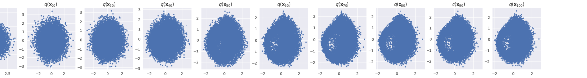
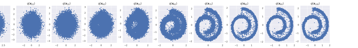
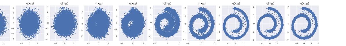
Figure 1: Data visualization for the training process. The rows correspond to epochs $400$, $1200$, and $2000$, respectively.

Fig. 1 visualizes the denoising and generative performance of the implemented diffusion model during training over swiss roll dataset with $10000$ samples. For this figure, we took “snapshots” by saving the model’s current state at specific checkpoints (every $400$ epochs) during the training process, and the corresponding output of the DDPM is plotted over time-steps $t=\{50,60,\ldots,100\}$. As can be seen from the figure, our DDPM gradually learns to denoise and generate samples out of an isotropic Gaussian distribution, where data samples with different levels of “noisiness” can be observed at different time-steps $t\in[T]$ from left to right. Moreover, as we reach the maximum number of epochs, the model can sooner (i.e., in fewer time-steps) generate samples.

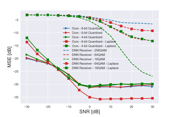
Figure 2: MSE between the original signal and the reconstructed one under AWGN channel and non-Gaussian additive noise.

We now study the performance of our system under low-SNR regimes, non-Gaussian additive noise, and quantization errors. Fig. 2 demonstrates the reconstruction performance of our DDPM-based scheme compared to the conventional DNN-based benchmark [7] over a wide range of SNR values. For this experiment, the original data samples are first qunatized into bitstreams, and then mapped to QAM symbols (as a widely-adopted constellation format in wireless networks [4, 2]) for transmission. The MSE metric (averaged over $10$ runs of sampling) between the original and the reconstructed data samples is considered for evaluation.

Since we have employed our DDPM at the receiver, we only exploit the receiver DNN of [7] and fine-tune it for benchmarking, in order to have a fair comparison. For the DNN benchmark, three linear layers with $64$ neurons at hidden layers and rectified linear unit (ReLU) activation functions are considered. For $16$- and $64$-QAM scenarios, we considered $5000$ training iterations, while for $256$-QAM, the DNN was trained for $30000$ iterations with Adam optimizer and learning rate $\lambda=0.01$. Notably, Fig. 2 highlights significant improvement in reconstruction performance among different quantization resolutions and across a wide range of SNR values, specially in low-SNR regimes. For instance, more than $25$ dB improvement is achieved at $0$ dB SNR for $64$-QAM scenario, compared to the the well-known model of [7] as one of the promising benchmarks in ML-based communications systems. Fig. 2 also highlights the resilience of our approach against non-Gaussian noise. In this experiment we consider additive Laplacian noise with the same variance as that of AWGN scenario [4]. The non-Gaussian noise can happen due to the non-Gaussian interference in multi user scenarios [4]. Remarkably, although we do not re-train our diffusion model under Laplacian noise, the performance of our approach does not change (or even becomes better) under this non-Gaussian assumption. However, we can see from the figure that the DNN benchmark can experience significant performance degradation under non-Gaussian assumption, although we have re-trained the DNN with Laplacian noise. This highlights the robust out-of-distribution performance of our proposed scheme.

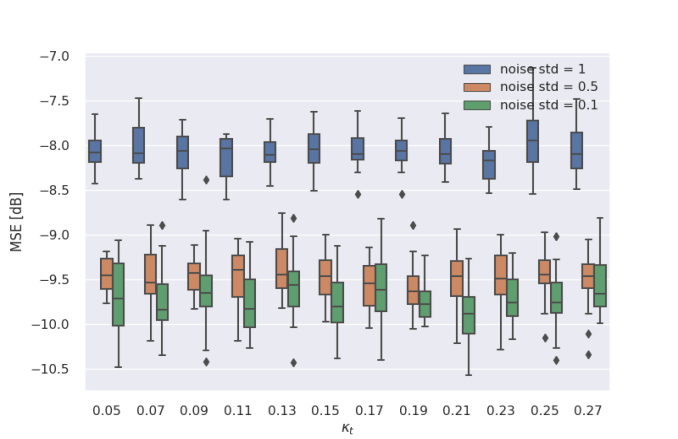
Figure 3: MSE between the original signal and the reconstructed one for different levels of hardware impairment over fading channels.

Fig. 3 studies the effect of different HWI levels on the reconstruction performance of our scheme over Rayleigh fading channels. For this figure, we set $\kappa^{t}=0.05$ and vary the impairment level of the receiver, $\kappa^{r}$, over the typical ranges specified in [16]. The reconstruction results are obtained in terms of MSE metric over $20$ realizations of the system. The figure highlights an important characteristic of our proposed scheme. Our DDPM-based communication system is resilient against hardware and channel distortions, as the reconstruction performance does not change with the increase in the impairment level. Notably, our DDPM-based scheme showcases a near-invariant reconstruction performance with respect to channel noise and impairment levels, which also highlights the generalizability of the proposed approach. This is achieved due to the carefully-designed so-called “variance scheduling” of our DDPM framework in (3), which allows the system to become robust against a wide range of distortions caused by channel and hardware impairments.

V Conclusions

In this paper, we have studied the application of DDPMs in wireless communication systems under HWIs. After introducing the DDPM framework and formulating our system model, we have evaluated the reconstruction performance of our scheme in terms of reconstruction performance. We have demonstrated the resilience of our DDPM-based approach under low-SNR regimes, non-Gaussian noise, and different HWI levels. Our results have shown that more than $25$ dB improvement in MSE is achieved compared to DNN-based receivers, as well as robust out-of-distribution performance.

References

- [1] P. Popovski. (2023, Jun. 11). “Communication engineering in the era of generative AI,” Medium, [Online]. Available: https://petarpopovski-51271.medium.com/communication-engineering-in-the-era-of-generative-ai-703f44211933
- [2] M. Merluzzi et al., “The Hexa-X project vision on artificial intelligence and machine learning-driven communication and computation co-design for 6G,” IEEE Access, vol. 11, pp. 65620–65648, Jun. 2023.
- [3] 3GPP Release 18, “Study on Artificial Intelligence (AI)/Machine Learning (ML) for NR Air Interface RAN,” Meeting #112, Athens, Greece, Tech. Rep., 27th February – 3rd March 2023.
- [4] M. Chafii, L. Bariah, S. Muhaidat, and M. Debbah, “Twelve scientific challenges for 6G: Rethinking the foundations of communications theory,” IEEE Communications Surveys & Tutorials, vol. 25, no. 2, pp. 868–904, Second quarter 2023.
- [5] Y. Liu, H. Du, D. Niyato, J. Kang, Z. Xiong, D. I. Kim, A. Jamalipour, “Deep generative model and its applications in efficient wireless network management: A tutorial and case study,” arXiv preprint arXiv: 2303.17114, Mar. 2023.
- [6] M. Honkala, D. Korpi, and J. M. J. Huttunen, “DeepRx: Fully convolutional deep learning receiver,” IEEE Transactions on Wireless Communications, vol. 20, no. 6, pp. 3925–3940, Jun. 2021.
- [7] F. A. Aoudia and J. Hoydis, “Model-free training of end-to-end communication systems,” IEEE Journal on Selected Areas in Communications, vol. 37, no. 11, pp. 2503–2516, Nov. 2019.
- [8] J. Ho, A. Jain, and P. Abbeel, “Denoising diffusion probabilistic models,” Advances in Neural Information Processing Systems, vol. 33, pp. 6840–6851, 2020.
- [9] B. Levac, A. Jalal, K. Ramchandran, and J. I. Tamir, “MRI reconstruction with side information using diffusion models,” arXiv preprint arXiv: 2303.14795, Jun. 2023.
- [10] M. Kim, R. Fritschek, and R. F. Schaefer, “Learning end-to-end channel coding with diffusion models,” 26th International ITG Workshop on Smart Antennas and 13th Conference on Systems, Communications, and Coding (WSA & SCC 2023), Braunschweig, Germany, Feb. 27 – Mar. 3, 2023, pp. 1–6.
- [11] M. Arvinte and J. I. Tamir, “MIMO channel estimation using score-based generative models,” IEEE Trans. Wireless Commun., vol. 22, no. 6, pp. 3698–3713, Jun. 2023.
- [12] X. Niu, X. Wang, D. Gündüz, B. Bai, W. Chen, and G. Zhou, “A hybrid wireless image transmission scheme with diffusion,” arXiv preprint arXiv: 2308.08244, Aug. 2023.
- [13] T. Wu, Z. Chen, D. He, L. Qian, Y. Xu, M. Tao, W. Zhang, “CDDM: Channel denoising diffusion models for wireless communications,” arXiv preprint arXiv: 2305.09161, May 2023.
- [14] A. Vaswani, et al., “Attention is all you need,” arXiv preprint arXiv: 1706.03762v7, Aug. 2023.
- [15] D. P. Kingma, T. Salimans, and M. Welling “Variational dropout and the local reparameterization trick,” Advances in Neural Information Processing Systems (NIPS 2015), vol. 28, 2015.
- [16] E. Björnson, J. Hoydis, M. Kountouris, and M. Debbah, “Massive MIMO systems with non-ideal hardware: Energy efficiency, estimation, and capacity limits,” IEEE Transactions on Information Theory, vol. 60, no. 11, pp. 7112–7139, Nov. 2014.
- [17] J. Hoydis, S. Cammerer, F. A. Aoudia, A. Vem, N. Binder, G. Marcus, and A. Keller, “Sionna: An open-source library for next-generation physical layer research,” arXiv preprint arXiv:2203.11854, Mar. 2023.
- [18] S. A. A. Kalkhoran, M. Letafati, E. Erdemir, B. H. Khalaj, H. Behroozi, and D. Gündüz, “Secure deep-JSCC against multiple eavesdroppers,” arXiv preprint arXiv: 2308.02892, Aug. 2023.