Automated dermatoscopic pattern discovery by clustering neural network output for human-computer interaction

Abstract

Background: As available medical image datasets increase in size, it becomes infeasible for clinicians to review content manually for knowledge extraction. The objective of this study was to create an automated clustering resulting in human-interpretable pattern discovery.

Methods: Images from the public HAM10000 dataset, including 7 common pigmented skin lesion diagnoses, were tiled into 29420 tiles and clustered via k-means using neural network-extracted image features. The final number of clusters per diagnosis was chosen by either the elbow method or a compactness metric balancing intra-lesion variance and cluster numbers. The amount of resulting non-informative clusters, defined as those containing less than six image tiles, was compared between the two methods.

Results: Applying k-means, the optimal elbow cutoff resulted in a mean of 24.7 (95%-CI: 16.4-33) clusters for every included diagnosis, including 14.9% (95% CI: 0.8-29.0) non-informative clusters. The optimal cutoff, as estimated by the compactness metric, resulted in significantly fewer clusters (13.4; 95%-CI 11.8-15.1; p=0.03) and less non-informative ones (7.5%; 95% CI: 0-19.5; p=0.017). The majority of clusters (93.6%) from the compactness metric could be manually mapped to previously described dermatoscopic diagnostic patterns.

Conclusions: Automatically constraining unsupervised clustering can produce an automated extraction of diagnostically relevant and human-interpretable clusters of visual patterns from a large image dataset.

Pre-peer review version

I Introduction

In dermatology, but also other visual medical fields, the recognition and description of specific samples of diseases is important for a precise diagnosis and for the formulation of differential diagnoses. Apart from clinical dermatology, there have been a plethora of pattern-descriptions of symptoms of disease in dermatoscopy in recent decades [1], especially for the diagnosis of skin tumors and inflammatory diseases [2], which are used for teaching and diagnosis in daily practice. These descriptions were mostly based on mono- or multicentric case collections that were reviewed manually by a few authors and evaluated on possible repetitions of patterns [3, 4, 5]. As clinical image data collections are increasing in size [6, 7], entirely manual review for discovering diagnostic patterns is not a realistic scenario anymore. In addition to an insurmountable workload, interrater disagreement may be a hindering factor in identifying and describing objective, valid and teachable pattern groups [1].

Increasingly, neural networks - especially convolutional neural networks (CNN) - are described as an aid for diagnostic classification of medical images. In the field of dermatology, CNNs were described to have at least an equal accuracy as dermatologists in experimental settings for classifying clinical and dermatoscopic images, and shown to improve physicians’ diagnostic accuracy when applied in diverse interactive settings [8, 9]. Such algorithms can not only classify images but also label anatomic areas [10], rate psoriasis [11], or retrieve similar images to a case, by implicitly analyzing patterns and pattern combinations after training to categorize images into distinct classes [12]. Therefore, we hypothesize that convolutional neural networks could be helpful in the extraction of diagnostically relevant patterns in medical image collections. Recent reports have shown unsupervised techniques when having limited label data [13].

The goal of this study was to create an automated workflow to extract diagnostic relevant pattern candidates for review by doctors and researchers, with dermatoscopic images of skin tumors as an example (Fig. 1). Eventually, from a big dataset with thousands of images, this should enable human-computer interaction and return an interpretable number of visually distinct patterns, by obtaining as few redundant or uninformative patterns as possible.

The approach we propose is a pipeline based on machine learning that consists of extracting deep features from CNNs, and applying an unsupervised clustering algorithm to these features. The clustering shall be constrained by a custom compactness metric that, in contrast to the well known elbow-metric, should better balance retrieval of all relevant patterns while at the same time keeping redundant information low.

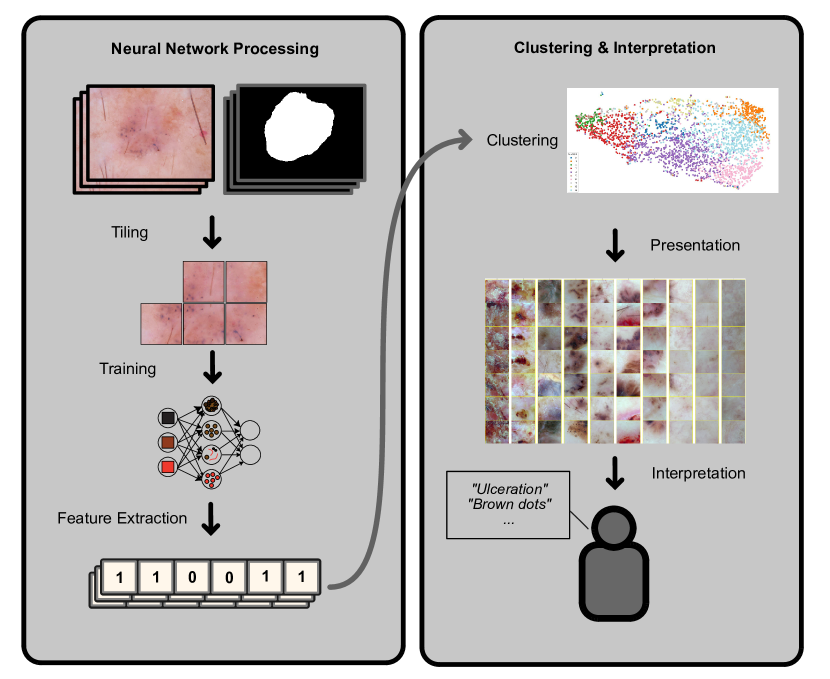
Figure 1: Processing overview - Dermatoscopic images (upper left) are used as source data, and a neural network is trained for classification on tiled lesion-area tiles. Features are extracted from lesion tiles with this trained network, on which an unsupervised k-means clustering is applied to find pattern groups. Up to the closest 7 lesion-tiles within a cluster (examples shown for clusters within the BCC class) are stored as representatives of a pattern and presented to a human reader for qualitative interpretation.

II Materials and Methods

II-A Data and processing

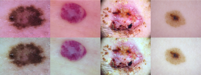
Figure S2: Top row shows original images from the HAM10000 dataset, and the bottom row results after color normalization.

This non-interventional retrospective study was conducted on public image data only, specifically the HAM10000 dataset [14]. This dataset is composed of 10015 dermatoscopic images of pigmented lesions with annotations on both the diagnosis and segmentation of the lesion area [8]. To focus on patterns rather than full images, analyses were performed on a tile-level. We extracted square subregions (tiles) of an image by a sliding window with a size of 128x128 pixels with 25% overlap, discarding tiles with $<60\%$ lesion area. In sum, 29420 tiles were extracted, Suppl. Fig. S1 shows two example cases with resulting extracted tiles, and Suppl. Table S1 the number of tiles per diagnosis. To ensure approximately equal representation of diagnoses, included nevi were limited to a random subsample of 1100 cases, and resulting tiles limited to a maximum random subsample of 850 tiles. To reduce the influence of changes in illumination color, we applied color constancy correction [15] to all tiles (Suppl. Fig. S2).

II-B Neural network and feature extraction

A VGG16 [16] architecture, pretrained on ImageNet data, was fine-tuned to classify tiles into one of seven diagnoses included in the HAM10000 dataset. Training was performed with all 29420 tiles, using 70% for training and the remaining 30% for validation during a single training run, ensuring no overlap of tiles of the same image between sets. This training run was only performed as a means to parameterize the model, thus as knowledge discovery rather than classification accuracy was the goal, the complete training dataset was also used for cluster analyses downstream. Data augmentation steps were flips in both horizontal and vertical directions, random 90º rotations, and zooms. Training was performed with a batch size of 32, using the Adam [17] optimizer, a weighted categorical cross entropy loss, with an initial learning rate of 1-e5, and an early stopping policy based on validation loss. For extracting features from image tiles by the fine-tuned model, the numerical state of the layer before the classification layer was obtained, resulting in a 1280-length vector. Neural network experiments were conducted using tensorflow [18] and python 3.8. Experiments were repeated with EfficientNet-B0 [19] and a convolutional autoencoder, with results for those two models shown in the supplementary data. For the autoencoder, we trained the model from scratch with a mean-squared error loss, and extracted the features from the flattened embedding space.

II-C Clustering

Resulting extracted features are normalized and used as input to an unsupervised clustering algorithm, specifically k-means [20] with cosine distance as a distance metric. This calculation was performed using scikit-learn v1.1.2 [21] and scipy v1.9.0 [22]. To automatically obtain the optimal number of clusters without further intervention from a user, either the elbow method (optimal value as calculated by yellowbrick v1.5 [23]) or a custom compactness metric (W) was applied. The latter method is based on the assumption that each lesion, thus also the tiles that comprise it, on average only show one or two dermatoscopic patterns. Thus, the proposed metric measures both the similarity of the clusters to which tiles of the same image have been assigned, and the number of different clusters the tiles were assigned to in respect to the total number of clusters. The metric was implemented as follows:

$$I=\left\{img_{1},...,img_{q}\right\}$$

$$T_{q}=\left\{t_{1},...,t_{j}\right\}$$

$$C_{q}=\left\{c_{1},...,c_{i}\right\}$$

$$W=\frac{1}{M}\times\sum_{q=1}^{M}\left(\frac{K}{min(n_{clst},L)}\times\sum_{L}^{j=1}cosDst\left(\frac{1}{K}\sum_{i=1}^{K}(c_{i}),t_{j}\right)\right)$$

where $M$ is the number of images $I$ in the experiment, $T_{q}$ are the $L$ tiles of an image $img_{q}$, $K$ is the number of unique clusters to which $T_{q}$ belong, $n_{clst}$ are the total number of clusters used in the experiment. Reiterating, the first half of W for an image ensures tiles are spread to as few clusters as possible, and the second half of W ensures the distance of tiles to the common center of clusters, that tiles are assigned to, is low.

II-D Classification ability

To assess classification ability of the two clustering cutoff methods, clusters were created not only for each diagnosis separately, but also for the whole dataset spanning all diagnoses. The frequency of diagnoses contained in a resulting cluster was noted as a multi-class probability for a classification task. Test images from the ISIC 2018 challenge Task 3 [24, 25] were tiled and preprocessed as above (resulting in 10254 tiles from 1304 lesions with sufficient lesion area depicted), and probabilities of the closest cluster of each tile averaged. The top-1 class of the resulting probabilities was taken as a prediction, and accuracy as well as mean recall [24] calculated.

II-E Manual pattern descriptions

Top-7 tiles of clusters, created for every diagnosis in the dataset separately with VGG16 feature vectors, k-means and the described compactness metric, were inspected by a dermatologist with substantial experience in dermatoscopy (PT). Patterns were scored for redundancy, i.e. showing the same pattern as another cluster of the diagnosis, informativeness, i.e. whether any reproducible pattern can be identified, number of patterns, and previous description, i.e. whether the pattern was already identified and described in the literature. A pattern was defined as a change in color and/or structure covering the majority of the image tile.

II-F Statistics

Differences of paired values were compared using a one-sample t-test after checking for normality assumptions. Statistical analyses were performed using R Statistics v4.1.0 [26], and plots created with ggplot2 [27]. A two sided p-value $<.05$ was regarded as statistically significant, with a Bonferroni-Holm type correction applied.

III Results

III-A Pattern interpretability

Applied on clusters of every diagnosis separately, the elbow method created a mean of 24.7 (95%-CI: 16.4-33) clusters for a diagnosis, whereas the compactness metric resulted in significantly less clusters (13.4; 95%-CI 11.8-15.1; p=0.03; Fig. 2(a)). The proportion of uninformative clusters was higher when using the elbow method (14.9%; 95% CI: 0.8-29.0) than using the compactness metric (7.5%, 95% CI: 0-19.5; p=0.017; Fig. 2(b)).

((a))

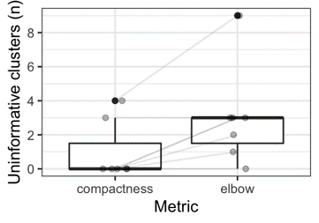
((b))

Figure 2: Number of overall (a) and uninformative (b) clusters per diagnosis when constraining cluster numbers via either the compactness or elbow method.

Qualitative interpretation of the clusters resulting from the compactness metric, for 93.6% (88 of 94) of diagnosis-specific clusters, at least one recognizable consistent pattern could be identified by a dermatologist. Identified patterns could be mapped to 53 unique known diagnostic descriptions from previous literature of at least 29 publications (Suppl. Table LABEL:supptab:qualitative_Annotation). Only 51 clusters could be described with one pattern alone, whereas 30 clusters encompassed two, and 7 clusters three recognizable patterns in combination. The proportion of redundant clusters within a diagnosis ranged from 0% (basal cell carcinoma and melanoma) to 27.3% (dermatofibroma and vascular lesions).

III-B Retained classification performance

Application of clustering on the whole dataset with all diagnoses included, using the elbow method resulted in a higher number of clusters than the compactness metric (42 vs. 7), as well as a higher mean recall (46.3 vs. 34.6) and accuracy (43.4%; 95%-CI 40.7-46.2 vs. 32.2%; 95%-CI 29.7-34.8) for predictions on the ISIC2018 test set. Clusters of the compactness metric were rarely able to predict actinic keratoses, and almost never dermatofibroma (Fig. 3).

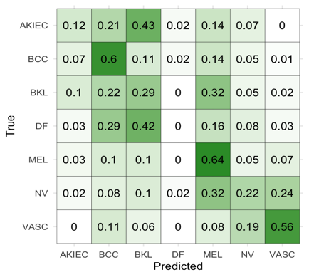
((a))

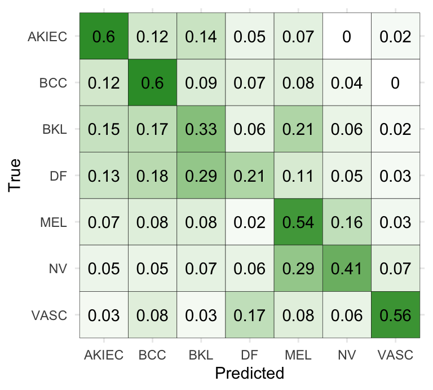
((b))

Figure 3: Confusion matrices showcasing performance of predictions via averaged nearest neighbor cluster-probabilities constrained by (a) compactness metric (7 clusters), or (b) the elbow method (42 clusters). Values within cells show proportions within one ground-truth class (=row).

IV Discussion

With ever growing image datasets, human interpretation of available data becomes increasingly difficult, and herein we present an automated analysis pipeline which via automated image processing is supposed to aid human-computer interaction for diagnostic marker discovery. Providing only information on the diagnosis and image area, we were able to showcase that the presented workflow is able to reproduce a major fraction of diagnostic patterns in dermatoscopy described in the literature.

In contrast to other publications [6, 24, 28] trying to optimize for the best diagnostic accuracy of a neural network model, herein we propose a metric to constrain k-means clustering to optimize for human interpretability in a truly interactive human-computer interaction workflow. The proposed compactness metric reduces the information to a digestible amount, shown by the significant reduction in overall clusters (Fig 2(a)), alongside a reduction of non-informative information shown by the significant reduction of noninformative clusters (Fig 2(b)). These improvements, though come at a cost, namely a reduced diagnostic accuracy when applied in an automated classification setting. This underlines that the training proposed herein could be useful for human-computer interaction and interpretability, but not for safely predicting diagnoses as a standalone application. As biases from automated predictions of image data through neural networks is a significant problem [29], datasets should be inspected for potential biases. Although not explicitly shown in this pilot experiment, the proposed workflow may enable medical personnel and researchers to identify highly prevalent biases in a qualitative manner. It is certainly not a complete solution, as based on the failure to classify rare classes (Fig 3(a)) we hypothesize that biases on rare classes will equally not be detectable.

Through qualitative analysis of resulting clusters we found that for most it is not possible to find a single pattern to describe them, but the majority needed at least a combination of two patterns (Supp. Table LABEL:supptab:qualitative_Annotation). This finding may help in designing future annotation and pattern analysis studies, and we hypothesize that studies trying to annotate and analyze for a single structure may not be representing real patterns. Interestingly, this may be a missing link between descriptive and “metaphoric” language [1], as the former is more suitable for distinct and concise descriptions, but metaphoric language inherently tries to capture structure combinations. A further interesting insight was that the frequency of redundant clusters was not equally distributed, but higher in dermatofibroma and vascular lesions. This could be sourced by the fact that these diagnoses in general show less variability in their patterns, but also that the used dataset through small sample size for these diagnoses is not covering the real visual variability. Finally, it is also interesting to note that by qualitatively comparing different network architectures (Supp. Fig. S4 - S10), one can identify different utility of them for the purpose of pattern discovery. While an Autoencoder is mainly detecting color blobs, edges, corners and curves, it is focussing less on detailed structures. The top-7 tiles from clusters created by using EfficientNetB0, as a representative of a modern architecture with higher diagnostic accuracy than VGG16 [19], were less homogeneous and thus harder to interpret. Thus, despite being not ideal for classification, we hypothesize that VGG16, through its inner architecture, is a well fit for extracting features of interpretable mid-level patterns useful for human-computer interaction. Future studies should show feasibility of implementation of this workflow not only for present dermatoscopic datasets [30], but also other imaging modalities such as dermatopathology and clinical images.

IV-A Limitations

This pilot study was supposed to showcase the general feasibility of the proposed process. Applicability to nonpigmented tumors, other localisations, inflammatory cases and darker skin types cannot be estimated as those were not included in the source datasets. The process at its core is analyzing substructures of dermatoscopic images, thus overall architecture is not integrated but could theoretically be overcome by changing the tile size and minimal lesion area. The latter is a relevant consideration when applying the workflow, as with the initially chosen tile size and lesion area constraints, some test cases with a very small lesion depicted did not produce any tile.

Data availability

Used image data are openly available at https://doi.org/10.7910/DVN/DBW86T (Harvard Dataverse). Resulting Clusters and qualitative evaluations are available in the supplementary material of this article.

Supplementary Data

Diagnosis	Nº images	Nº Tiles
AKIEC	327	2993
BCC	514	2989
BKL	1099	7992
DF	115	825
MEL	1113	8262
NV	6705	5927
VASC	142	432

Table S1: Correspondence between the number of images of the HAM10000 dataset according to diagnosis with the number of tiles extracted and used during the experimentation.

		Elbow	Compactness
Diagnosis	Feature extraction model	optimal nº of clusters	optimal nº of clusters
	EfficientNet B0	23	18
	VGG16	23	13
AKIEC	AE	38	12
	EfficientNet B0	17	14
	VGG16	24	10
BCC	AE	34	15
	EfficientNet B0	21	15
	VGG16	28	16
BKL	AE	33	18
	EfficientNet B0	17	10
	VGG16	11	14
DF	AE	24	14
	EfficientNet B0	40	16
	VGG16	25	14
MEL	AE	45	13
	EfficientNet B0	35	12
	VGG16	41	14
NV	AE	49	13
	EfficientNet B0	15	18
	VGG16	21	13
VASC	AE	24	20
	EfficientNet B0	28	10
	VGG16	42	7
All	AE	34	6

Table S2: Resulting cluster numbers by diagnosis, model and clustering cutoff method. W denotes the compactness value.

Table S3: Qualitative annotation data of clusters via top-7 tiles.

Diagnosis	Cluster num. (arbitrary)	Inconclusive	Pattern 1	Pattern 2	Pattern 3	Redundant to	Term from previous literature	Literature
	1	0	dots, grey, linear	vessels, red, linear			Dots-as-lines	[5]
	6	0	circles, white	lines, grey/brown, angulated			Angulated lines	[31]
	12	0	structureless, brown				Structureless brown	[32]
	9	0	circles, white	structureless, brown			White circles	[32]
	2	0	follicles, skin- colored, prominent	structureless, brown			Prominent follicles	[33]
	11	0	structureless, white				Structureless white	[5]
	5	0	circles, white	structureless, brown	hair, black, thick	9	White circles	[31]
	3	0	follicles, skin- colored, prominent	structureless, brown, angulated	dots, grey		Prominent follicles	[31]
AKIEC	8	0	structureless, brown	telangiectasia, red, blurry			Linear-wavy vessels	[34]
	7	0	structureless, brown	dots, brown			Brown dots and structureless	[5]
	4	0	structureless, brown, linear				-
	10	0	structureless, brown, clustered				Structureless brown, clusters	[5]
	0	0	dots, brown, linear			1	Dots-as-lines	[5]
	3	0	structures, white	telangiectasia, red, blurry			Shiny white structures	[35]
	2	0	structureless, skin-colored	telangiectasia, red, blurry			Shiny white structures	[35]
	4	0	structureless, pink	reticular lines, brown, delicate			Network-like structures	[36]
	7	0	clod, brown, radial/peripheral (?leaf like?)				Leaf-like	[37]
	6	1	lesion border
	5	0	clod, brown/blue, in another clod	structureless, white/pink, as background			Clod within a clod	[1]
	8	0	clod, brown/blue, in another clod	structureless, brown, as background			Clod within a clod	[1]
BCC	1	1	structureless, purple				Blue-gray globules	[38]
	9	0	clod, red/orange	structureless, pink	structures, white		Ulceration	[38]
	0	0	structureless, white/orange/red				Ulceration	[38]
	6	0	structureless, brown/grey, speckled				Granular pattern	[39]
	15	0	structureless, brown/grey				Blotch	[4]
	5	0	structureless, brown/red	clods, orange/skin-colored			Comedo-like openings	[4]
	8	0	structureless, brown/grey				Blotch	[4]
	10	0	structureless, brown	lesion border, sharp demarcation			Sharp demarcation	[4]
	11	0	structureless, brown, speckled	reticular lines, brown			?False? reticular lines	[40]
	1	0	dots, grey				Coarse granules	[41]
	2	0	dots, brown	structureless, brown			Coarse granules	[41]
	13	0	reticular lines, brown, thick				Thickened network	[4]
BKL	3	0	clods, purple, with central vessel				Exophytic papillary structure	[4]
	14	0	structureless, light brown				Blotch	[4]
	12	0	curved lines, brown, thick				fat fingers	[42]
	4	1	circles, brown				-
	9	0	structureless, brown	reticular lines, brown, uneven		11	?False? reticular lines	[40]
	7	0	structureless, brown	dots, brown, single			Granular pattern	[39]
	0	0	structureless, blue/grey				Blotch	[4]
	3	0	structureless, brown	structureless, white, central			Central white scarlike tile	[43]
	4	0	structureless, red, prominent skin markings				Reddish coloration	[43]
	11	0	structureless, brown, central white/red			3	Central white scarlike tile	[43]
	6	0	structureless, red/skin-colored	scaling, white, delicate			Reddish coloration	[43]
	1	0	reticular lines, brown, delicate and broken up				Pigment network	[43]
	8	1	-				-
	9	0	structureless, red	scaling, white/orange, dense/peripheral circular			Scale crusts	[43]
	13	1	-				-
	5	0	structureless, brown	structureless, white/pink, in corner		3	Central white scarlike tile	[43]
DF	10	0	structureless, brown/skin-colored				-
	7	0	clods, brown				Brown globules	[43]
	12	0	clods, brown			7	Brown globules	[43]
	2	0	structureless, white/pink, parallel linear arrangement				-
	0	1	-				-
	7	0	structureless, brown/grey				Grey structures	[31]
	1	0	structureless, brown				Light brown structureless areas	[44]
	4	0	structureless, skin-colored	telegeangiectasia, pink, blurry			Depigmentation	[45]
	9	0	reticular lines, brown	structureless, brown	lines, white		White scar-like areas	[45]
	11	0	structureless, black/grey				Blue-black pigmentation	[46]
	13	0	colors, brown/black/white				Blue-white veil	[47]
	6	0	reticular lines, brown, uneven	dots, grey	lesion border, scalloped		Regression	[47]
	12	0	structureless, brown, uneven distribution				Nonuniform pigment distribution	[44]
	10	0	structureless, blue	dots, brown, single			Streaks	[47]
	5	0	reticular lines, brown, focal hyperpigmentation				Mistletoe sign	[48]
MEL	2	0	lines, brown, angulated				Angulated lines	[49]
	8	0	lines, brown, radial/peripheral				Irregular extensions	[50]
	3	1	reticular lines, brown, thick				-
	0	0	reticular lines, brown, uneven in structure and color				Irregular pigment network	[50]
	10	0	structureless, light brown				Homogeneous pattern	[51]
	3	0	reticular lines, brown, smooth border transition	structureless, brown	follicle openings, skin colored		Typical pigment network	[52]
	1	0	reticular lines, brown, smooth border transition	structureless, brown		3	Typical pigment network	[52]
	13	0	reticular lines, brown, smooth border transition	structureless, brown		3	Typical pigment network	[52]
	11	0	reticular lines, brown	clods, brown, single			Brown globules	[52]
	2	0	reticular lines, grey, delicate	structureless, grey			-
	9	0	clods, brown/skin- colored, with central vessel	scaling, white, delicate			Globular pattern	[52]
	7	0	structureless, brown, hypopigmented areas				White scar-like areas	[45]
	12	0	reticular lines, brown/black				Superficial black network	[52]
	4	0	lesion border, brown, eccentric hyperpigmen- tation				Mistletoe sign	[48]
NV	5	1	structureless, brown, hypopigmented areas	clods, brown			-
	6	0	reticular lines, brown, uneven in structure and color	lesion border, scalloped			Irregular pigment network	[50]
	8	0	reticular lines, brown, uneven in structure			6	Irregular pigment network	[50]
	0	1	-				-
	11	0	clods, blue				Red-blue lacunae	[53]
	1	0	clods, red, clustered				Red globules	[53]
	2	0	structureless, red, skin- colored septae				White rail	[54]
	8	0	structureless, red, skin- colored septae			2	White rail	[54]
	5	0	clods, red, not in focus				Red lacunae	[53]
	12	0	clods, red, not in focus			5	Red lacunae	[53]
	10	0	structureless, red, skin- colored septae			2	White rail	[54]
	6	0	clod, red, cicular skin- colored demarcation				White collarette	[54]
	9	1	-				-
	4	1	-				-
VASC	3	0	clods, purple	scaling, white, dense	clods, black, in scaling (?blood clods?)		Hemorrhagic crusts	[55]
	7	0	structureless, blue				Red-blue lacunae	[53]
	0	0	structureless, blue, skin- colored septae				Dark lacunae & Whitish veil	[55]

Figure S1: Example of the tiles extracted (right) from the images of the HAM10000 dataset (left) following the sliding window strategy and that compose our dataset.

AKIEC		Clusters
VGG16	Elbow
	Compactness
Autoencoder	Elbow
	Compactness
EfficientNetB0	Elbow
	Compactness

Table S4: Clusters resulting from AKIEC diagnosis for each network model (VGG16, Autoencoder, EfficientNetB0) and cluster constraint (Elbow, Compactness). A maximum of 7 tiles closest to the cluster center are shown.

BCC		Clusters
VGG16	Elbow
	Compactness
Autoencoder	Elbow
	Compactness
EfficientNetB0	Elbow
	Compactness

Table S5: Clusters resulting from BCC diagnosis for each network model (VGG16, Autoencoder, EfficientNetB0) and cluster constraint (Elbow, Compactness). A maximum of 7 tiles closest to the cluster center are shown.

BKL		Clusters
VGG16	Elbow
	Compactness
Autoencoder	Elbow
	Compactness
EfficientNetB0	Elbow
	Compactness

Table S6: Clusters resulting from BKL diagnosis for each network model (VGG16, Autoencoder, EfficientNetB0) and cluster constraint (Elbow, Compactness). A maximum of 7 tiles closest to the cluster center are shown.

DF		Clusters
VGG16	Elbow
	Compactness
Autoencoder	Elbow
	Compactness
EfficientNetB0	Elbow
	Compactness

Table S7: Clusters resulting from DF diagnosis for each network model (VGG16, Autoencoder, EfficientNetB0) and cluster constraint (Elbow, Compactness). A maximum of 7 tiles closest to the cluster center are shown.

MEL		Clusters
VGG16	Elbow
	Compactness
Autoencoder	Elbow
	Compactness
EfficientNetB0	Elbow
	Compactness

Table S8: Clusters resulting from MEL diagnosis for each network model (VGG16, Autoencoder, EfficientNetB0) and cluster constraint (Elbow, Compactness). A maximum of 7 tiles closest to the cluster center are shown.

NV		Clusters
VGG16	Elbow
	Compactness
Autoencoder	Elbow
	Compactness
EfficientNetB0	Elbow
	Compactness

Table S9: Clusters resulting from NV diagnosis for each network model (VGG16, Autoencoder, EfficientNetB0) and cluster constraint (Elbow, Compactness). A maximum of 7 tiles closest to the cluster center are shown.

VASC		Clusters
VGG16	Elbow
	Compactness
Autoencoder	Elbow
	Compactness
EfficientNetB0	Elbow
	Compactness

Table S10: Clusters resulting from VASC diagnosis for each network model (VGG16, Autoencoder, EfficientNetB0) and cluster constraint (Elbow, Compactness). A maximum of 7 tiles closest to the cluster center are shown.

References

- [1] H. Kittler, A. A. Marghoob, G. Argenziano, C. Carrera, C. Curiel-Lewandrowski, R. Hofmann-Wellenhof, J. Malvehy, S. Menzies, S. Puig, H. Rabinovitz et al., “Standardization of terminology in dermoscopy/dermatoscopy: Results of the third consensus conference of the international society of dermoscopy,” Journal of the American Academy of Dermatology, vol. 74, no. 6, pp. 1093–1106, 2016.
- [2] E. Errichetti, I. Zalaudek, H. Kittler, Z. Apalla, G. Argenziano, R. Bakos, A. Blum, R. Braun, D. Ioannides, F. Lacarrubba et al., “Standardization of dermoscopic terminology and basic dermoscopic parameters to evaluate in general dermatology (non-neoplastic dermatoses): an expert consensus on behalf of the international dermoscopy society,” British Journal of Dermatology, vol. 182, no. 2, pp. 454–467, 2020.
- [3] S. W. Menzies, K. Westerhoff, H. Rabinovitz, A. W. Kopf, W. H. McCarthy, and B. Katz, “Surface microscopy of pigmented basal cell carcinoma,” Archives of dermatology, vol. 136, no. 8, pp. 1012–1016, 2000.
- [4] R. P. Braun, H. S. Rabinovitz, J. Krischer, J. Kreusch, M. Oliviero, L. Naldi, A. W. Kopf, and J. H. Saurat, “Dermoscopy of pigmented seborrheic keratosis: a morphological study,” Archives of dermatology, vol. 138, no. 12, pp. 1556–1560, 2002.
- [5] A. Cameron, C. Rosendahl, P. Tschandl, E. Riedl, and H. Kittler, “Dermatoscopy of pigmented bowen’s disease,” Journal of the American Academy of Dermatology, vol. 62, no. 4, pp. 597–604, 2010.
- [6] S. S. Han, M. S. Kim, W. Lim, G. H. Park, I. Park, and S. E. Chang, “Classification of the clinical images for benign and malignant cutaneous tumors using a deep learning algorithm,” Journal of Investigative Dermatology, vol. 138, no. 7, pp. 1529–1538, 2018.
- [7] M. Combalia, N. C. Codella, V. Rotemberg, B. Helba, V. Vilaplana, O. Reiter, C. Carrera, A. Barreiro, A. C. Halpern, S. Puig et al., “Bcn20000: Dermoscopic lesions in the wild,” arXiv preprint arXiv:1908.02288, 2019.
- [8] P. Tschandl, C. Rinner, Z. Apalla, G. Argenziano, N. Codella, A. Halpern, M. Janda, A. Lallas, C. Longo, J. Malvehy et al., “Human–computer collaboration for skin cancer recognition,” Nature Medicine, vol. 26, no. 8, pp. 1229–1234, 2020.
- [9] S. S. Han, I. Park, S. E. Chang, W. Lim, M. S. Kim, G. H. Park, J. B. Chae, C. H. Huh, and J.-I. Na, “Augmented intelligence dermatology: deep neural networks empower medical professionals in diagnosing skin cancer and predicting treatment options for 134 skin disorders,” Journal of Investigative Dermatology, vol. 140, no. 9, pp. 1753–1761, 2020.
- [10] L. Amruthalingam, P. Gottfrois, A. Gonzalez Jimenez, B. Gökduman, M. Kunz, T. Koller, D. Consortium, M. Pouly, A. Navarini, J.-T. Maul et al., “Improved diagnosis by automated macro-and micro-anatomical region mapping of skin photographs,” Journal of the European Academy of Dermatology and Venereology, vol. 36, no. 12, pp. 2525–2532, 2022.
- [11] T. Okamoto, M. Kawai, Y. Ogawa, S. Shimada, and T. Kawamura, “Artificial intelligence for the automated single-shot assessment of psoriasis severity,” Journal of the European Academy of Dermatology and Venereology, vol. 36, no. 12, pp. 2512–2515, 2022.
- [12] P. Tschandl, G. Argenziano, M. Razmara, and J. Yap, “Diagnostic accuracy of content-based dermatoscopic image retrieval with deep classification features,” British Journal of Dermatology, vol. 181, no. 1, pp. 155–165, 2019.
- [13] S. Krammer, Y. Li, N. Jakob, A. Boehm, H. Wolff, P. Tang, T. Lasser, L. French, and D. Hartmann, “Deep learning-based classification of dermatological lesions given a limited amount of labelled data,” Journal of the European Academy of Dermatology and Venereology, vol. 36, no. 12, pp. 2516–2524, 2022.
- [14] P. Tschandl, C. Rosendahl, and H. Kittler, “The ham10000 dataset, a large collection of multi-source dermatoscopic images of common pigmented skin lesions,” Scientific data, vol. 5, no. 1, pp. 1–9, 2018.
- [15] C. Barata, M. E. Celebi, and J. S. Marques, “Improving dermoscopy image classification using color constancy,” IEEE journal of biomedical and health informatics, vol. 19, no. 3, pp. 1146–1152, 2014.
- [16] K. Simonyan and A. Zisserman, “Very deep convolutional networks for large-scale image recognition,” arXiv preprint arXiv:1409.1556, 2014.
- [17] D. P. Kingma and J. Ba, “Adam: A method for stochastic optimization,” arXiv preprint arXiv:1412.6980, 2014.
- [18] M. Abadi, A. Agarwal, P. Barham, E. Brevdo, Z. Chen, C. Citro, G. S. Corrado, A. Davis, J. Dean, M. Devin et al., “Tensorflow: Large-scale machine learning on heterogeneous distributed systems,” arXiv preprint arXiv:1603.04467, 2016.
- [19] M. Tan and Q. Le, “Efficientnet: Rethinking model scaling for convolutional neural networks,” in International conference on machine learning. PMLR, 2019, pp. 6105–6114.
- [20] J. A. Hartigan and M. A. Wong, “Algorithm as 136: A k-means clustering algorithm,” Journal of the royal statistical society. series c (applied statistics), vol. 28, no. 1, pp. 100–108, 1979.
- [21] F. Pedregosa, G. Varoquaux, A. Gramfort, V. Michel, B. Thirion, O. Grisel, M. Blondel, P. Prettenhofer, R. Weiss, V. Dubourg et al., “Scikit-learn: Machine learning in python,” the Journal of machine Learning research, vol. 12, pp. 2825–2830, 2011.
- [22] P. Virtanen, R. Gommers, T. E. Oliphant, M. Haberland, T. Reddy, D. Cournapeau, E. Burovski, P. Peterson, W. Weckesser, J. Bright et al., “Scipy 1.0: fundamental algorithms for scientific computing in python,” Nature methods, vol. 17, no. 3, pp. 261–272, 2020.
- [23] B. Bengfort and R. Bilbro, “Yellowbrick: Visualizing the scikit-learn model selection process,” Journal of Open Source Software, vol. 4, no. 35, p. 1075, 2019.
- [24] P. Tschandl, N. Codella, B. N. Akay, G. Argenziano, R. P. Braun, H. Cabo, D. Gutman, A. Halpern, B. Helba, R. Hofmann-Wellenhof et al., “Comparison of the accuracy of human readers versus machine-learning algorithms for pigmented skin lesion classification: an open, web-based, international, diagnostic study,” The lancet oncology, vol. 20, no. 7, pp. 938–947, 2019.
- [25] N. Codella, V. Rotemberg, P. Tschandl, M. E. Celebi, S. Dusza, D. Gutman, B. Helba, A. Kalloo, K. Liopyris, M. Marchetti et al., “Skin lesion analysis toward melanoma detection 2018: A challenge hosted by the international skin imaging collaboration (isic),” arXiv preprint arXiv:1902.03368, 2019.
- [26] R Core Team, R: A Language and Environment for Statistical Computing, R Foundation for Statistical Computing, Vienna, Austria, 2023. [Online]. Available: https://www.R-project.org/
- [27] H. Wickham and H. Wickham, “Data analysis,” ggplot2: elegant graphics for data analysis, pp. 189–201, 2016.
- [28] H. A. Haenssle, C. Fink, F. Toberer, J. Winkler, W. Stolz, T. Deinlein, R. Hofmann-Wellenhof, A. Lallas, S. Emmert, T. Buhl et al., “Man against machine reloaded: performance of a market-approved convolutional neural network in classifying a broad spectrum of skin lesions in comparison with 96 dermatologists working under less artificial conditions,” Annals of oncology, vol. 31, no. 1, pp. 137–143, 2020.
- [29] M. Groh, C. Harris, L. Soenksen, F. Lau, R. Han, A. Kim, A. Koochek, and O. Badri, “Evaluating deep neural networks trained on clinical images in dermatology with the fitzpatrick 17k dataset,” in Proceedings of the IEEE/CVF Conference on Computer Vision and Pattern Recognition, 2021, pp. 1820–1828.
- [30] P. Zaballos, S. Puig, A. Llambrich, and J. Malvehy, “Dermoscopy of dermatofibromas: a prospective morphological study of 412 cases,” Archives of dermatology, vol. 144, no. 1, pp. 75–83, 2008.
- [31] P. Tschandl, C. Rosendahl, and H. Kittler, “Dermatoscopy of flat pigmented facial lesions,” Journal of the European Academy of Dermatology and Venereology, vol. 29, no. 1, pp. 120–127, 2015.
- [32] M. Inskip, A. Cameron, B. N. Akay, M. Gorji, S. P. Clark, N. Rosendahl, M. Coetzer-Botha, H. Kittler, and C. Rosendahl, “Dermatoscopic features of pigmented intraepidermal carcinoma on the head and neck,” JDDG: Journal der Deutschen Dermatologischen Gesellschaft, vol. 18, no. 9, pp. 969–976, 2020.
- [33] K. Peris, T. Micantonio, D. Piccolo, and M. Concetta, “Dermoscopic features of actinic keratosis,” JDDG: Journal der Deutschen Dermatologischen Gesellschaft, vol. 5, no. 11, pp. 970–975, 2007.
- [34] I. Zalaudek, J. Giacomel, G. Argenziano, R. Hofmann-Wellenhof, T. Micantonio, A. Di Stefani, M. Oliviero, H. Rabinovitz, H. Soyer, and K. Peris, “Dermoscopy of facial nonpigmented actinic keratosis,” British Journal of Dermatology, vol. 155, no. 5, pp. 951–956, 2006.
- [35] M. Scalvenzi, S. Lembo, M. G. Francia, and A. Balato, “Dermoscopic patterns of superficial basal cell carcinoma,” International journal of dermatology, vol. 47, no. 10, pp. 1015–1018, 2008.
- [36] A. Gulia, D. Altamura, S. De Trane, T. Micantonio, M. C. Fargnoli, and K. Peris, “Pigmented reticular structures in basal cell carcinoma and collision tumours,” British Journal of Dermatology, vol. 162, no. 2, pp. 442–444, 2010.
- [37] M. Püspök-Schwarz, A. Steiner, M. Binder, B. Partsch, K. Wolff, and H. Pehamberger, “Statistical evaluation of epiluminescence microscopy criteria in the differential diagnosis of malignant melanoma and pigmented basal cell carcinoma.” Melanoma research, vol. 7, no. 4, pp. 307–311, 1997.
- [38] K. Peris, E. Altobelli, A. Ferrari, M. C. Fargnoli, D. Piccolo, M. Esposito, and S. Chimenti, “Interobserver agreement on dermoscopic features of pigmented basal cell carcinoma,” Dermatologic surgery, vol. 28, no. 7, pp. 643–645, 2002.
- [39] L. Bugatti and G. Filosa, “Dermoscopy of lichen planus-like keratosis: a model of inflammatory regression,” Journal of the European Academy of Dermatology and Venereology, vol. 21, no. 10, pp. 1392–1397, 2007.
- [40] V. De Giorgi, D. Massi, M. Stante, and P. Carli, “False “melanocytic” parameters shown by pigmented seborrheic keratoses: a finding which is not uncommon in dermoscopy,” Dermatologic surgery, vol. 28, no. 8, pp. 776–779, 2002.
- [41] P. Zaballos, S. Blazquez, S. Puig, E. Salsench, J. Rodero, J. Vives, and J. Malvehy, “Dermoscopic pattern of intermediate stage in seborrhoeic keratosis regressing to lichenoid keratosis: report of 24 cases,” British Journal of Dermatology, vol. 157, no. 2, pp. 266–272, 2007.
- [42] A. W. Kopf, H. Rabinovitz, A. Marghoob, R. P. Braun, S. Wang, M. Oliviero, and D. Polsky, ““fat fingers:” a clue in the dermoscopic diagnosis of seborrheic keratoses,” Journal of the American Academy of Dermatology, vol. 55, no. 6, pp. 1089–1091, 2006.
- [43] A. Ferrari, H. P. Soyer, K. Peris, G. Argenziano, G. Mazzocchetti, D. Piccolo, V. De Giorgi, and S. Chimenti, “Central white scarlike patch: a dermatoscopic clue for the diagnosis of dermatofibroma,” Journal of the American Academy of Dermatology, vol. 43, no. 6, pp. 1123–1125, 2000.
- [44] G. Annessi, R. Bono, F. Sampogna, T. Faraggiana, and D. Abeni, “Sensitivity, specificity, and diagnostic accuracy of three dermoscopic algorithmic methods in the diagnosis of doubtful melanocytic lesions: the importance of light brown structureless areas in differentiating atypical melanocytic nevi from thin melanomas,” Journal of the American Academy of Dermatology, vol. 56, no. 5, pp. 759–767, 2007.
- [45] M. A. Pizzichetta, G. Argenziano, R. Talamini, D. Piccolo, A. Gatti, G. Trevisan, G. Sasso, A. Veronesi, A. Carbone, and H. P. Soyer, “Dermoscopic criteria for melanoma in situ are similar to those for early invasive melanoma,” Cancer, vol. 91, no. 5, pp. 992–997, 2001.
- [46] E. Rodríguez-Lomba, B. Lozano-Masdemont, L. M. Nieto-Benito, E. H. de la Torre, R. Suárez-Fernández, and J. A. Avilés-Izquierdo, “Dermoscopic predictors of tumor thickness in cutaneous melanoma: a retrospective analysis of 245 melanomas,” Dermatology Practical & Conceptual, vol. 11, no. 3, 2021.
- [47] G. Argenziano, G. Fabbrocini, P. Carli, V. De Giorgi, E. Sammarco, and M. Delfino, “Epiluminescence microscopy for the diagnosis of doubtful melanocytic skin lesions: comparison of the abcd rule of dermatoscopy and a new 7-point checklist based on pattern analysis,” Archives of dermatology, vol. 134, no. 12, pp. 1563–1570, 1998.
- [48] G. Kamińska-Winciorek, P. Właszczuk, and J. Wydmański, ““mistletoe sign”: probably a new dermoscopic descriptor for melanoma in situ and melanocytic junctional nevus in the inflammatory stage,” Advances in Dermatology and Allergology/Postkepy Dermatologii i Alergologii, vol. 30, no. 5, pp. 316–319, 2013.
- [49] N. Jaimes, A. A. Marghoob, H. Rabinovitz, R. P. Braun, A. Cameron, C. Rosendahl, G. Canning, and J. Keir, “Clinical and dermoscopic characteristics of melanomas on nonfacial chronically sun-damaged skin,” Journal of the American Academy of Dermatology, vol. 72, no. 6, pp. 1027–1035, 2015.
- [50] H. Soyer, J. Smolle, G. Leitinger, E. Rieger, and H. Kerl, “Diagnostic reliability of dermoscopic criteria for detecting malignant melanoma,” Dermatology, vol. 190, no. 1, pp. 25–30, 1995.
- [51] R. Hofmann-Wellenhof, A. Blum, I. H. Wolf, D. Piccolo, H. Kerl, C. Garbe, and H. P. Soyer, “Dermoscopic classification of atypical melanocytic nevi (clark nevi),” Archives of dermatology, vol. 137, no. 12, pp. 1575–1580, 2001.
- [52] G. Argenziano, H. P. Soyer, S. Chimenti, R. Talamini, R. Corona, F. Sera, M. Binder, L. Cerroni, G. De Rosa, G. Ferrara et al., “Dermoscopy of pigmented skin lesions: results of a consensus meeting via the internet,” Journal of the American Academy of Dermatology, vol. 48, no. 5, pp. 679–693, 2003.
- [53] J. Gao, W. Fei, C. Shen, X. Shen, M. Sun, N. Xu, Q. Li, C. Huang, T. Zhang, R. Ko et al., “Dermoscopic features summarization and comparison of four types of cutaneous vascular anomalies,” Frontiers in Medicine, vol. 8, p. 692060, 2021.
- [54] P. Zaballos, A. Llambrich, F. Cuéllar, S. Puig, and J. Malvehy, “Dermoscopic findings in pyogenic granuloma,” British Journal of Dermatology, vol. 154, no. 6, pp. 1108–1111, 2006.
- [55] P. Zaballos, C. Daufí, S. Puig, G. Argenziano, D. Moreno-Ramírez, H. Cabo, A. A. Marghoob, A. Llambrich, I. Zalaudek, and J. Malvehy, “Dermoscopy of solitary angiokeratomas: a morphological study,” Archives of dermatology, vol. 143, no. 3, pp. 318–325, 2007.