Topological Node2vec: Enhanced Graph Embedding via Persistent Homology

Abstract.

Node2vec is a graph embedding method that learns a vector representation for each node of a weighted graph while seeking to preserve relative proximity and global structure. Numerical experiments suggest Node2vec struggles to recreate the topology of the input graph. To resolve this we introduce a topological loss term to be added to the training loss of Node2vec which tries to align the persistence diagram (PD) of the resulting embedding as closely as possible to that of the input graph. Following results in computational optimal transport, we carefully adapt entropic regularization to PD metrics, allowing us to measure the discrepancy between PDs in a differentiable way. Our modified loss function can then be minimized through gradient descent to reconstruct both the geometry and the topology of the input graph. We showcase the benefits of this approach using demonstrative synthetic examples.

1. Introduction

Various data types, such as bodies of text or weighted graphs, do not come equipped with a natural linear structure, complicating or outright preventing the use of most machine learning techniques that typically require Euclidean data as input. A natural workaround for this is to find a way to represent such data as sets of points in some Euclidean space $\mathbb{R}^{m}$. Regarding bodies of text, any unique word appears throughout a text with its own frequency and propensity for having certain neighbors or forming certain grammatical structures. This information can be used to assign each word some $m$-dimensional point in a way such that relative proximities of all these points maximally respect the neighborhood and structural data of the text. This is precisely the point of the Word2vec model (Mikolov et al., 2013).

Node2vec (Grover and Leskovec, 2016) and its predecessor Deepwalk (Perozzi et al., 2014) learn representations of all the nodes in a weighted graph as Euclidean points in a fixed dimension. These are essentially Word2vec models in which each node of the input graph is given context in a ‘sentence’ by taking random walks starting from that node. This random-walk-generated training data is then handled in precisely the same way Word2vec would handle words surrounded by sentences. This construction is easy to alter and expand upon, allowing it to appear in complex projects like the one to embed new multi-contact (hypergraph) cell data, as seen in the general work (Zhang et al., 2020a) and then specialized to biological purposes in the follow-up paper (Zhang and Ma, 2020).

While representation learning models prove useful for revitalizing existing analyses and opening up new insights, it is important to understand the extent of the data loss under such a transformation. In this paper, we identify an area of stark failure on the part of Node2vec (or more generally, random-walk-based graph embeddings) to retain certain graph properties and so reintroduce the ability to resolve such features via the inclusion of a new loss function. This failure point and the loss function we introduce to compensate for it are both topological in nature.

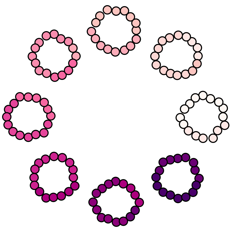
(a)

(b)

(c)

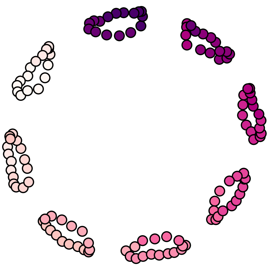
(d)

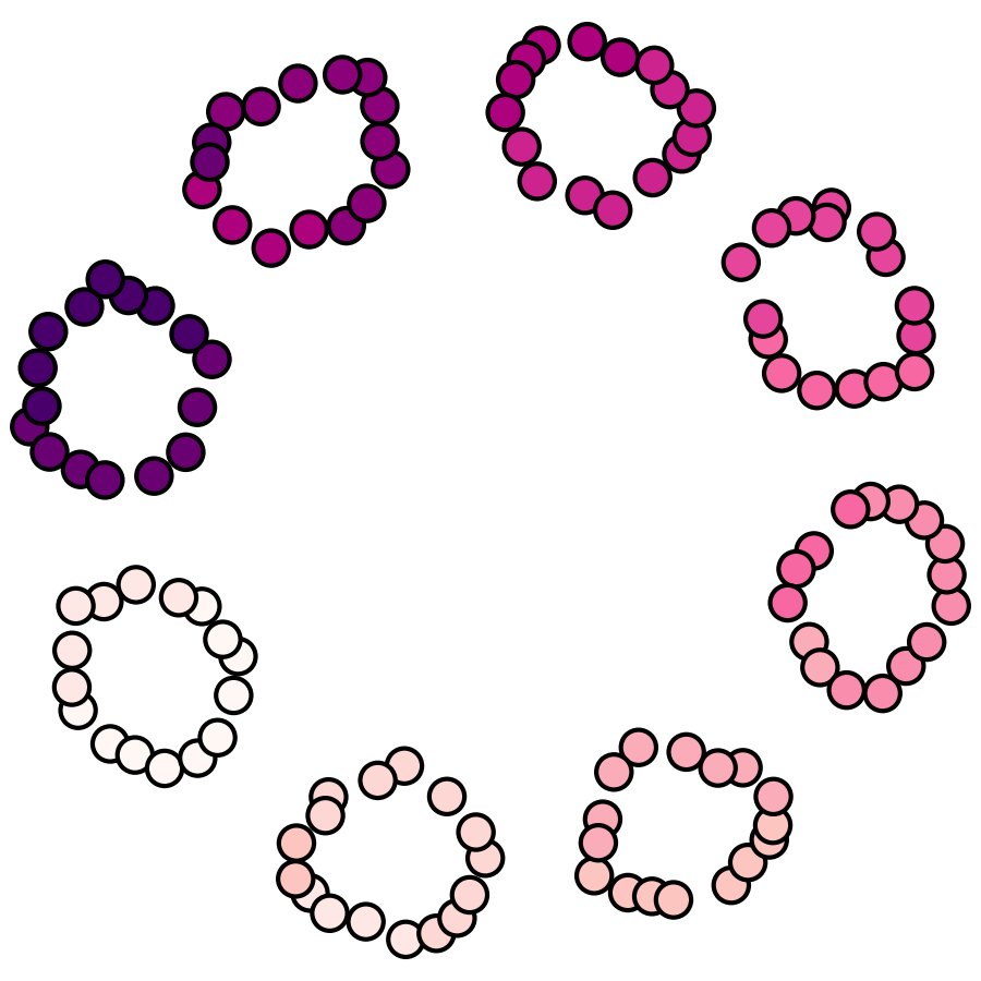
(e)

Figure 1. Illustration of Node2vec behavior with and without the incorporation of our topological loss during training. (a) An initial point cloud and (b) its corresponding pairwise distance matrix. (c) The weighted adjacency matrix obtained by inverting the pairwise distances. This is the graph used as input for Node2vec in this experiment. (d) The embedding proposed by Node2vec after training using only the standard reconstruction loss. It fails to properly retrieve the eight smaller cycles appearing in the input graph, and the emergent central cycle is far too large. (e) The embedding proposed by Node2vec after training while including our new topological loss term, in which the eight smaller cycles are recovered and the central cycle has been kept to a proper size.

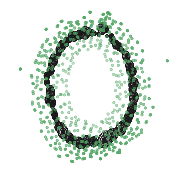
(a)

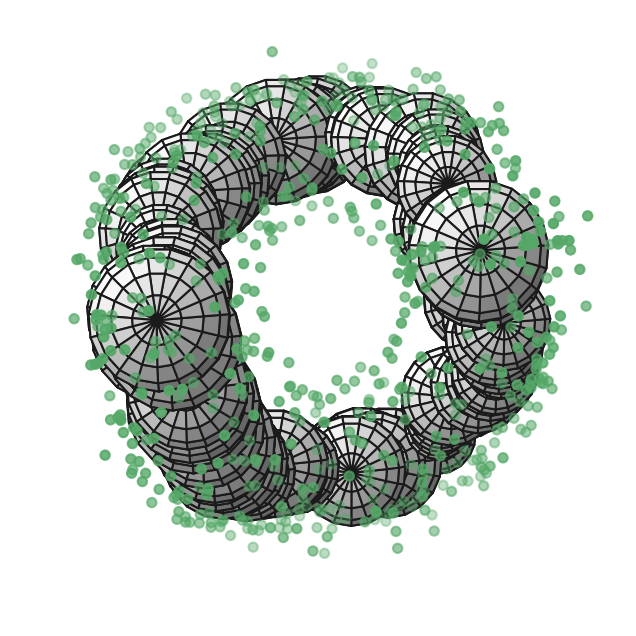
(b)

Figure 2. Illustration of Node2vec behavior on a torus with and without the incorporation of our topological loss during training. (a) View of the final embedding proposed by Node2vec using only the standard reconstruction loss, seen from ‘above’. The transparency of points represents the distance from the observer in the $z$-axis. Drawn in black are the largest inscribable spheres constructed at discretized angle increments around the center of the data set. The tubelike topology of the torus is all but erased. (b) View of the final embedding proposed by Node2vec including our new topological loss term with the largest inscribable spheres drawn inside. The tubelike topology of the torus is recovered.

1.1. Related Works

Graph embeddings. We have already mentioned the existence and value of graph-representation models which use as training data some node neighborhood information. This training data can be prescribed via random walks (Perozzi et al., 2014; Grover and Leskovec, 2016) or other criteria (Tang et al., 2015), after which it is fed into a ‘skip gram’ encoder framework as in (Mikolov et al., 2013) to learn a representation.

There are many node-to-vector representation learning models with various emphases or improvements on the general framework, for example: the work of (Bojchevski and Günnemann, 2018) which represents each node as a Gaussian distribution to capture uncertainty; MDS (Torgerson, 1952) which has existed for the better part of a century and presently refers to a category of matrix algorithms for representing an input distance matrix (reciprocal of a graph’s adjacency matrix) as a set of Euclidean points; neighborhood methods that eschew a skip-gram model for direct matrix factorization (Cao et al., 2015); and (Ou et al., 2016) leveraging data-motivated symmetries in directed graphs. We refer to (Cui et al., 2018; Xu, 2021) for comprehensive surveys of such methods.

While we focus on Node2vec as an easily implemented, flexible, and widely used baseline, our method can be applied in parallel with any graph representation method from which a persistence diagram can be computed at every epoch. This is trivially the case for any method learning an Euclidean representation, such as node-to-vector representation models.

Topological optimization. In order to incorporate topological information into the training of Node2vec, we rely on Topological Data Analysis (TDA), a branch of algebraic topology rooted in the works (Edelsbrunner et al., 2000; Zomorodian and Carlsson, 2005). Persistent homology in particular provides topological descriptors called persistence diagrams that summarize the topological information (connected components, loops, cavities, etc.) of structured objects (point clouds, graphs, etc.). These diagrams are frequently compared through partial matching metrics (Cohen-Steiner et al., 2005, 2010). The question of optimizing topology is introduced in (Gameiro et al., 2016). It has found different practical applications such as shape matching (Poulenard et al., 2018), surface reconstruction (Brüel-Gabrielsson et al., 2020), graph classification (Yim and Leygonie, 2021), and topological regularization of machine learning models (Chen et al., 2019; Hu et al., 2019; Gabrielsson et al., 2020).

While many applications see topology being applied to the abstract inner layers of machine learning frameworks for normalization or noise reduction (Hensel et al., 2021), in our application, as in the setting of (Moor et al., 2020), every step of the learning process proposes a constantly improving Euclidean data-set from which we can directly obtain (and compare) topologies via persistent homology.

Important theoretical results related to our work are (Carriere et al., 2021), which establishes the local convergence of stochastic gradient descents of loss functions that incorporate the comparison of topological descriptors, and (Leygonie et al., 2021) which provides a chain rule that enables explicit computation of gradients of topological terms.

Topological optimization is an active research area and recent variants have been proposed to mitigate some of its limitations: (Leygonie et al., 2023) shows that the non-smoothness of the persistent homology map can be alleviated by leveraging its stratified structure, and Nigmetov and Morozov (2022) propose a way to address the sparsity of topological gradients. In this work, we propose another way of improving the behavior of topological loss functions by adding a specially designed entropic regularization term, an idea inspired by advancements in computational optimal transport.

Optimal transport for TDA. Optimal transport literature can be traced back to the works of Monge (1781) and Kantorovich (1942). (We refer to the bibliography of (Villani, 2009) for a comprehensive overview of optimal transport history.) The optimal transportation problem is a linear program whose goal is to optimize matchings, thus sharing important similarities with the metrics used in TDA to compare persistence diagrams (Mileyko et al., 2011; Turner et al., 2014). This connection has been made explicit in (Divol and Lacombe, 2021a) and leveraged toward statistical applications in a series of works (Divol and Lacombe, 2021b; Cao and Monod, 2022). During the last decade, the work of Cuturi (2013) has popularized the use of an entropic regularization term (an idea that can be traced back to the work of Schrödinger (1932)) which makes the resulting optimization problem strictly convex and hence more efficient to solve, along with ensuring differentiable solutions with respect to the input objects. This opened the door to a wide range of practical applications, see for instance (Solomon et al., 2015; Benamou et al., 2015). The entropic optimal transport problem has been further refined through the introduction of so-called Sinkhorn divergences, initially utilized on a heuristic basis (Ramdas et al., 2017; Genevay et al., 2018) and then further studied in (Feydy et al., 2019; Séjourné et al., 2019). A direct use of entropic optimal transport in TDA was first investigated in (Lacombe et al., 2018). However, it has recently been observed in (Lacombe, 2023) that the problem introduced in the former work suffers from inhomogeneity. The latter, more recent work introduces a new regularized transportation problem that can be applied to TDA metrics while preserving the important properties of Sinkhorn divergences (efficient computation, differentiability) and which we further build upon in the present work.

1.2. Contributions and Outline

Section 2 discusses preliminary technicalities required to properly introduce the Node2vec model. We describe the simplest implementation of the Node2vec model and carefully derive the gradient of the training loss. Section 3 introduces the topological loss function which will be used to incorporate topological information into the Node2vec model. In particular, we apply a recently introduced entropic regularization of metrics used to compare topological descriptors based on ideas developed in the computational optimal transport community and carefully derive the corresponding gradient. To the best of our knowledge, this is the first use of entropic regularization in the context of topological optimization. Gathering these results, Section 4 presents the modified algorithm we use to train this new Topological Node2vec model. We provide numerical results in Section 5, elaborating on the results in Figures 1 and 2 to demonstrate that the addition of topological information significantly improves the quality of embeddings. Our implementation is publicly available at this repository.

2. The Node2vec Model

Node2vec is a machine learning model that learns the representation of a graph’s nodes as a set of Euclidean points in some specified dimension. We carefully explain the neighborhood generation methodology characteristic to Node2vec (based on Word2vec and Deepwalk) and the structure of Node2vec’s internal parameters, as well as derive the gradient of its loss function.

We elaborate on the details of Node2vec in this section following the structure laid out in Algorithm 1. Node2vec learns an embedding in $\mathbb{R}^{m}$ of a graph by minimizing a loss function $L_{0}$ that measures some distance between the currently proposed embedding (initially random) and training data extracted from the input graph.

Algorithm 1 Node2vec algorithm

a weighted graph $G=(V,E,w)$, learning rate $\eta>0$, embedding dimension $m$, neighborhood parameters $(l,r,p,q)$;

$\mathbb{P}\subset\mathbb{R}^{m}$ with $|\mathbb{P}|=|V|$

• initialize the parameter matrices $\Theta(0)$ (Definition 1) with values uniformly sampled from the interval $(-1,1)$; let $k=0$;

while not converged do

     • for each node $v\in V$, generate the current neighborhood vector $C_{v}$ (Definition 2) and the training neighborhood vector $T_{v}$ (Eq. (3)); let $C(k)=\{C_{v}(k)\}_{v\in V}$ and $T(k):=\{T_{v}(k)\}_{v\in V}$

     • update $\Theta(k+1)$ using the gradient result of Proposition 1:

$$\Theta(k+1):=\Theta(k)-\eta\nabla_{\Theta(k)}L_{0}(T(k),C(k))$$

     • $k\mathrel{+}=1$

end while

We consider in this work weighted, undirected graphs, referred to simply as graphs, as represented by a tuple $G=(V,E,w)$, where $V=\{v_{1},\ldots,v_{n}\}$ is a set of vertices with a total order, $E=V\times V$, and $w:E\to\mathbb{R}_{\geq 0}$ is a symmetric weight function (i.e., $w(v_{i},v_{j})=w(v_{j},v_{i})$ for all $1\leq i<j\leq n$) into the set of non-negative real numbers.

Definition 1 (Node2vec structure).

Let $G=(V,E,w)$ be a graph, $|V|=n$ denote the number of nodes, and $m\in\mathbb{N}$ be the desired embedding dimension. Define $\Theta:=\{W_{1},W_{2}\}$ where $W_{1}\in\mathcal{M}_{n\times m}(\mathbb{R})$ and $W_{2}\in\mathcal{M}_{m\times n}(\mathbb{R})$ are matrices of size $n\times m$ and $m\times n$, respectively. Let $W_{1}(i,\cdot)$ denote the $i$^th row of the matrix $W_{1}$ for $1\leq i\leq n$. The corresponding Node2vec embedding is defined as

$$\mathrm{Emb}(\Theta)=\{W_{1}(i,\cdot)\}_{1\leq i\leq n}\subset\mathbb{R}^{m}.$$

When necessary, we will write $\Theta(k),\mathrm{Emb}(\Theta(k))$ to convey dependence on the epoch $k$ during the learning process.

Definition 2 (Current neighborhood probability).

For $v=v_{i}\in V$, given some parameter matrices $\Theta$, the current predicted neighborhood probability of $v$ is the vector $C_{v}$ given by the following: Let $\bar{v}=(0,\ldots,0,1,0,\ldots,0)\in\mathbb{R}^{n}$ be the row vector where $\bar{v}(i)=1$, and for all $1\leq j\leq n$ with $j\neq i$, $\bar{v}(j)=0$. Define

(1) $$u(=u_{v}):=\bar{v}\cdot{W_{1}}\cdot{W_{2}}\in\mathbb{R}^{n}$$

and subsequently let $C_{v}$ be the softmax of $u$:

$$C_{v}=\left(\frac{e^{u(1)}}{\sum_{1\leq j\leq n}e^{u(j)}},\ldots,\frac{e^{u(n)}}{\sum_{1\leq j\leq n}e^{u(j)}}\right).$$

For a node $v\in V$, the training neighborhood probability vector $T_{v}$ is generated through the following process: Four parameters are needed to dictate how $T_{v}$ is generated:

• $r$: the number of random walks to be generated starting from the node $v$,

• $l$: the length of each walk,

• $p$: a parameter that determines how often a walk will return to the previous vertex in the walk,

• $q$: a parameter that determines how often a walk will move to a new vertex that is not a neighbor of the previous vertex.

We generate $r$ walks starting from $v$, each of length $l$, with probability transitions given the parameters $p,q$ and weight function $w:E\to\mathbb{R}_{\geq 0}$. Specifically:

• For the first step of the walk, the probability of traveling to any node $v_{\textrm{next}}$ is the normalized edge weight

  $$\frac{w(v,v_{\textrm{next}})}{\sum_{\hat{v}\in V}w(v,\hat{v})}.$$

• Suppose the previous step in the walk was $v_{\textrm{prev}}\to v_{\textrm{curr}}$. For any node $v_{\textrm{next}}\in V$, define

  $$\xi(v_{\textrm{prev}},v_{\textrm{curr}},v_{\textrm{next}})=\left\{\begin{array}[]{ll}0&\text{if }w(v_{\textrm{curr}},v_{\textrm{next}})=0\\ 1/p&\text{if }w(v_{\textrm{curr}},v_{\textrm{next}})\neq 0\text{ and }v_{\textrm{prev}}=v_{\textrm{next}}\\ 1&\text{if }w(v_{\textrm{curr}},v_{\textrm{next}})\neq 0\text{, }v_{\textrm{prev}}\neq v_{\textrm{next}}\text{, and }w(v_{\textrm{prev}},v_{\textrm{next}})>0\\ 1/q&\text{otherwise}.\end{array}\right.$$

Then, the probability of choosing any $v_{\textrm{next}}$ as the next node in the walk is

(2) $$\frac{{\xi(v_{\textrm{prev}},v_{\textrm{curr}},v_{\textrm{next}})}\cdot w(v_{\textrm{curr}},v_{\textrm{next}})}{\sum_{\hat{v}\in V}\xi(v_{\textrm{prev}},v_{\textrm{curr}},\hat{v})\cdot w(v_{\textrm{curr}},\hat{v})}.$$

Collect all the nodes traversed by the $r$ random walks starting from $v$ and save this information in a multiplicity function $t_{v}:V\to\mathbb{Z}_{\geq 0}$. That is, for any node $v_{j}\in V$, $t_{v}(v_{j})$ is equal to the number of times this node was reached across all the random walks starting from $v$.

Finally, represent the information of the multiplicity function $t$ as a probability vector indexed over all the nodes of $V$:

(3) $$T_{v}=\left(\frac{t_{v}(v_{j})}{l\cdot r}\right)_{1\leq j\leq n}.$$

When necessary, we will write this vector as $T_{v}(k)$ to convey dependence on the epoch $k$ during the learning process.

Remark 1.

It is also possible to neglect this random walk process and simply take $T_{v}$ to be the normalization of the vector $(w(v_{1},v),\ldots,w(v_{n},v)).$ This is equivalent to the parameter choice of $l=1$ and $r=\infty$. The choice of $p$ and $q$ have no impact on walks of length $l=1$. This captures immediate neighborhood information and fails to see structures such as hubs and branches. However, as showcased later in our experiments, there are situations in which this is a computationally superior option.

Node2vec is trained by minimizing the following loss $L_{0}$:

(4) $$\Theta\mapsto L_{0}(T,\Theta):=\sum_{v\in V}H(T_{v},C_{v}),$$

where $H$ denotes the cross-entropy between probability distributions, given by

$$H(A,B)=-\sum_{y\in Y}A(y)\log B(y)$$

with the convention that $0\log(0)=0$. A practical formula to express this loss is given by the following lemma:

Lemma 1 (Grover and Leskovec (2016), Equation (2)).

Let $v\in V$. Treating $C_{v}$ and $T_{v}$ as probability distributions over $V$,

$$H(T_{v},C_{v})=-\sum_{1\leq j\leq n}T_{v}(j)u_{v}(j)+\log\sum_{1\leq j\leq n}e^{u_{v}(j)},$$

where $u_{v}$ is as defined in (1).

The minimization of (4) is performed through gradient descent, for which we provide an explicit expression below. In the following proposition, we use $M(\cdot,\cdot)$ to denote matrix coordinates in order to avoid excessive subscripting. We also make use of the Kronecker delta notation where for comparable objects $a,b$, $\delta_{a,b}=1$ if $a=b$ and $0$ otherwise.

Proposition 1.

Recall that $\Theta=(W_{1},W_{2})$. Then, the gradient of $L_{0}$ with respect to $W_{1}$ is

$$\nabla_{W_{1}}L_{0}(T,\Theta)=\left[\sum_{1\leq i\leq n}\delta_{v_{i},v_{l}}\cdot\sum_{1\leq a\leq n}W_{2}(j,a)(C_{v_{i}}(a)-T_{v_{i}}(a))\right]_{\begin{subarray}{c}1\leq l\leq n\\ 1\leq j\leq m\end{subarray}}.$$

Also, the gradient of $L_{0}$ with respect to $W_{2}$ is

$$\nabla_{W_{2}}L_{0}(T,\Theta)=\left[\sum_{1\leq i\leq n}W_{1}(i,j)(C_{v_{i}}(l)-T_{v_{i}}(l))\right]_{\begin{subarray}{c}1\leq l\leq n\\ 1\leq j\leq m\end{subarray}}.$$

The proof of this result is deferred to the appendix.

3. A Topological Loss Function for Node2vec

This section presents the important background on topological data analysis required in this work, including the computation of topological descriptors called persistence diagrams (PD) and their comparison through entropy regularized metrics. Eventually, we derive an explicit gradient for these metrics that we will use when training Node2vec with a topological term in its reconstruction loss.

Essentially, we will include a topological loss term $L_{1}$ when training Node2vec (see Eq. (4)) which penalizes the difference between the PD of Node2vec’s output and the PD of the input graph.

3.1. From Point Clouds to Persistence Diagrams

Persistent homology identifies topological features in structured objects such as point clouds and encodes them as discrete measures called persistence diagrams, supported on the open half-plane $\Omega=\{(b,d)\in\mathbb{R}^{2},\ d>b\}$. Each point in these measures expresses the scales within the original point cloud at which a given topological feature was created (born) and destroyed (died). We refer to (Chazal et al., 2016; Edelsbrunner and Harer, 2022) for a general introduction. Below, we provide a concise presentation of this theory specialized to the context of our work.

Let $\mathbb{P}=\{p_{1},\ldots,p_{n}\}\subset\mathbb{R}^{m}$ be a finite point cloud. The Vietoris-Rips complex of parameter $\rho$, denoted $\mathrm{VR}_{\rho}$, is the simplicial complex over $\mathbb{P}$ given by all simplices such that the longest pairwise distance between the vertices of that simplex is at most $\rho$. Increasing $\rho$ from $0$ to the diameter of the point cloud gives us the filtration of simplicial complexes $\mathrm{VR}=\{\mathrm{VR}_{\rho}\}$. A topological feature is one that is enclosed at some $\rho_{\textrm{birth}}$ (a hollow space enclosed by edges, a hollow void enclosed by triangles, etc.) and then eventually filled in by higher dimensional simplices at some $\rho_{\textrm{death}}>\rho_{\textrm{birth}}$. We call $\rho_{\textrm{birth}}$ and $\rho_{\textrm{death}}$ the birth and death values of the topological feature, respectively.

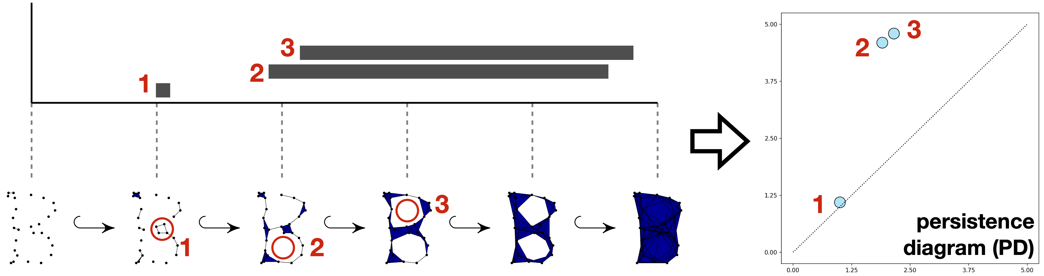
Figure 3. Vietoris-Rips construction of the filtered simplicial complex on a 2D point cloud. The persistence diagram represents topological features as points in the upper diagonal half-plane of $\mathbb{R}^{2}$. Points close to the diagonal such as point $1$ above (birth and death values are very close) are regarded as noise. Features far from the diagonal, such as points $2$ and $3$, persist across a large range of scales and are considered significant.

We say a point cloud is in Vietoris-Rips general position when all of the birth and death values of all topological features are unique. The persistence diagram of $\mathbb{P}$ is the multiset $\mathrm{PD}(\mathbb{P})=\{x_{i}=(b_{x_{i}},d_{x_{i}})\}_{1\leq i\leq N}\subset\Omega$ collecting all the birth and death values of topological features of $\mathbb{P}$ (See Figure 3). Equivalently, this information can be represented as the finite counting measure $\alpha=\sum_{i=1}^{N}\delta_{x_{i}}$, where $\delta_{x_{i}}$ denotes the Dirac mass located at $x_{i}$.

3.2. Metrics for PDs and Optimal Transport

We now elucidate the development of metrics in optimal transport (OT) regarding how they can be applied to measuring the distance between persistence diagrams (PDs). In the following, we adopt the representation of PDs as finite counting measures, a formalism initially introduced in (Chazal et al., 2016) which is vital for discussing connections to OT literature.

We denote the orthogonal projection of $x\in\Omega$ to the diagonal $\partial\Omega:=\{(b,b),\ b\in\mathbb{R}\}$ by $p_{\partial\Omega}(x)$.

Definition 3.

The space $\mathcal{D}$ of persistence diagrams is the set of finite counting measures supported on $\Omega$, that is

$$\mathcal{D}=\left\{\alpha=\sum_{i=1}^{N}\delta_{x_{i}}\ \big{|}\ x_{i}\in\Omega,N\in\mathbb{N}\right\}.$$

We equip $\mathcal{D}$ with the metric $(\alpha,\beta)\mapsto\mathrm{FG}(\alpha,\beta)^{\frac{1}{2}}$ (Cohen-Steiner et al., 2010) expressed as the square-root of

(5) $$\mathrm{FG}(\alpha,\beta)=\inf_{\zeta\in\Xi(\alpha,\beta)}\sum_{x}\|x-\zeta(x)\|^{2},$$

where $\Xi(\alpha,\beta)$ denotes the set of bijections from $\mathrm{supp}(\alpha)\cup\partial\Omega$ to $\mathrm{supp}(\beta)\cup\partial\Omega$, and $\mathrm{supp}(\mu)$ denotes the support of a counting measure $\mu$ (i.e. the set of all $x$ such that $\mu(\{x\})>0$). Such a $\zeta$ essentially bijects a subset of $\alpha$ onto a subset of $\beta$ while mapping all leftover points to the diagonal $\partial\Omega$. We call $\zeta$ a partial matching between $\alpha$ and $\beta$. Any $\zeta^{*}\in\Xi(\alpha,\beta)$ that achieves the infimum in (5) is said to be an optimal partial matching between $\alpha$ and $\beta$.

Remark 2.

In practice, persistence diagrams come with an essential component which consists of points whose death coordinate is $+\infty$. In the context of Vietoris-Rips filtrations built on top of arbitrary point clouds, there is exactly one such point in the persistence diagram of the form $(0,+\infty)$. We ignore this for the purposes of our analysis.

Remark 3.

In the TDA literature, the metric $\mathrm{FG}(\cdot,\cdot)^{\frac{1}{2}}$ is often referred to as the Wasserstein distance between persistence diagrams (see, e.g., (Cohen-Steiner et al., 2010; Turner et al., 2014)), using an analogy with the Wasserstein distance introduced in OT literature (Villani, 2009; Santambrogio, 2015; Peyré et al., 2019). A formal connection between these two concepts was established in (Divol and Lacombe, 2021a), where it was shown that the metric used in TDA is equivalent to the optimal transport problem with Dirichlet boundary condition introduced by Figalli and Gigli (2010). We use the notation $\mathrm{FG}$ to stress that this metric is not equivalent to the Wasserstein distance used in OT. Adapting tools from OT literature to PDs (entropic regularization, gradients) will require this level of technical care.

The following reformulation of $\mathrm{FG}$ will be convenient going forward:

Proposition 2 ((Divol and Lacombe, 2021a; Lacombe, 2023)).

Let $\alpha,\beta\in\mathcal{D}$ be two persistence diagrams with $\alpha=\sum_{i=1}^{N}\delta_{x_{i}}$ and $\beta=\sum_{j=1}^{M}\delta_{y_{j}}$. The (squared) distance between $\alpha$ and $\beta$ can be rephrased as the following minimization problem:

(6) $$\mathrm{FG}(\alpha,\beta)=\inf_{P\in\Pi} \bigg{[}\sum_{\begin{subarray}{c}1\leq i\leq N,\\ 1\leq j\leq M\end{subarray}}\|x_{i}-y_{j}\|^{2}P_{ij}$$

$$+\sum_{i=1}^{N}\|x_{i}-p_{\partial\Omega}(x_{i})\|^{2}\left(1-\sum_{j=1}^{M}P_{ij}\right)$$

$$+\sum_{j=1}^{M}\|y_{j}-p_{\partial\Omega}(y_{j})\|^{2}\left(1-\sum_{i=1}^{N}P_{ij}\right)\bigg{]},$$

where

(7) $$\Pi=\left\{P\in\mathbb{R}_{\geq 0}^{N\times M},\ \forall i\in\{1,\dots,N\},\forall j\in\{1,\dots,M\},\ \sum_{i^{\prime}=1}^{N}P_{i^{\prime}j}\leq 1,\sum_{j^{\prime}=1}^{M}P_{ij^{\prime}}\leq 1\right\}.$$

The main claim of Proposition 2 is that the infimum over bijections $\zeta$ in (5) can be relaxed to a minimization over matrices $P$ that satisfy sub-marginal constraints as a consequence of Birkoff’s theorem. Such a $P$ will be referred to as a partial transport plan.

3.3. Entropic Regularization for PD Metrics

While theoretically appealing, the metric $\mathrm{FG}$ has drawbacks. It is computationally expensive and, though the optimal matching $\zeta^{*}$ is generically unique, it suffers from instability: a small perturbation in $\alpha$ can significantly change $\zeta^{*}$, which is a clearly undesirable behavior when it comes to optimizing topological losses (as detailed in section 3.4).

In computational optimal transport, an alternative approach popularized by Cuturi (2013) consists of introducing a regularization term based on entropy. An illustrative translation of this idea into the context of PD metrics would be to consider the following adjusted problem from Proposition 2:

(8) $$\text{minimize }P\mapsto\bigg{[} \sum_{\begin{subarray}{c}1\leq i\leq N,\\ 1\leq j\leq M\end{subarray}}\|x_{i}-y_{j}\|^{2}P_{ij}$$

$$+\sum_{i=1}^{N}\|x_{i}-p_{\partial\Omega}(x_{i})\|^{2}\left(1-\sum_{j=1}^{M}P_{ij}\right)$$

$$+\sum_{j=1}^{M}\|y_{j}-p_{\partial\Omega}(y_{j})\|^{2}\left(1-\sum_{i=1}^{N}P_{ij}\right)$$

$$+\epsilon\mathrm{KL}(P|1_{NM})\bigg{]},$$

where $P\in\Pi$, $\epsilon>0$ is the ‘regularization parameter’, $1_{NM}$ denotes the matrix of size $N\times M$ filled with $1$s, and $\displaystyle\mathrm{KL}(A|B)=\sum_{\begin{subarray}{c}1\leq i\leq N,\\ 1\leq j\leq M\end{subarray}}A_{ij}\log\left(\frac{A_{ij}}{B_{ij}}\right)-A_{ij}+B_{ij}$ for any two matrices $A,B\in\mathbb{R}^{N\times M}$. In (Lacombe et al., 2018) it was shown that, just like its OT counterpart, (8) can be solved by the Sinkhorn algorithm (Sinkhorn, 1964), a simple iterative algorithm that is highly parallelizable and GPU-friendly.

However, an important observation made in (Lacombe, 2023) is that (8) is not $1$-homogeneous in $(\alpha,\beta)$ when $\epsilon>0$ (while the same equation with $\epsilon=0$ is). While this is of no consequence to the typical OT practitioner (see (Lacombe, 2023, Section 3)), it dramatically affects persistence diagrams, which may have highly disparate total masses. Loosely speaking, when $N,M$ are large, the entropic contribution tends to outweigh the transport cost in (8), yielding transportation plans that concentrate near the diagonal. To overcome this behavior, we propose the following version of entropic regularization for PD metrics, building on Homogeneous Unbalanced Regularized OT (HUROT) (Lacombe, 2023):

Definition 4.

Let $\alpha=\sum_{i=1}^{N}\delta_{x_{i}},\beta=\sum_{j=1}^{M}\delta_{y_{j}}\in\mathcal{D}$ and $\epsilon>0$. The HUROT problem $\mathrm{FG}_{\epsilon}$ between $\alpha$ and $\beta$ is defined as

(9) $$\mathrm{FG}_{\epsilon}(\alpha,\beta):=\inf_{P\in\Pi} \bigg{[}\sum_{\begin{subarray}{c}1\leq i\leq N,\\ 1\leq j\leq M\end{subarray}}\|x_{i}-y_{j}\|^{2}P_{ij}$$

$$+\sum_{i=1}^{N}\|x_{i}-p_{\partial\Omega}(x_{i})\|^{2}\left(1-\sum_{j=1}^{M}P_{ij}\right)$$

$$+\sum_{j=1}^{M}\|y_{j}-p_{\partial\Omega}(y_{j})\|^{2}\left(1-\sum_{i=1}^{N}P_{ij}\right)$$

$$+\epsilon R(P|\mathbf{a}\mathbf{b}^{T})\bigg{]},$$

where $\Pi$ is defined in (7) and the vectors $\mathbf{a}=(\|x_{i}-p_{\partial\Omega}(x_{i})\|^{2})_{i=1}^{N}\in\mathbb{R}^{N}$ and $\mathbf{b}=(\|y_{j}-p_{\partial\Omega}(y_{j})\|^{2})_{j=1}^{M}\in\mathbb{R}^{M}$ are both treated as column vectors, resulting in $\mathbf{a}\mathbf{b}^{T}$ being a $N\times M$ matrix. The homogeneous entropic regularization term is given by

(10) $$R(P|\mathbf{a}\mathbf{b}^{T}):=\frac{1}{2}\left(\mathrm{KL}\left(P\bigg{|}\frac{\mathbf{a}\mathbf{b}^{T}}{\mathrm{pers}(\alpha)}\right)+\mathrm{KL}\left(P\bigg{|}\frac{\mathbf{a}\mathbf{b}^{T}}{\mathrm{pers}(\beta)}\right)\right)$$

where $\displaystyle\mathrm{pers}(\alpha)=\sum_{i=1}^{N}\|x_{i}-p_{\partial\Omega}(x_{i})\|^{2}$ is called the total persistence of $\alpha$ (and similarly for $\beta$).

We additionally define the Sinkhorn divergence between persistence diagrams to be

(11) $$\mathrm{SFG}_{\epsilon}(\alpha,\beta):=\mathrm{FG}_{\epsilon}(\alpha,\beta)-\frac{1}{2}\mathrm{FG}_{\epsilon}(\alpha,\alpha)-\frac{1}{2}\mathrm{FG}_{\epsilon}(\beta,\beta).$$

The main benefit of working with $\mathrm{FG}_{\epsilon}$ instead of $\mathrm{FG}$ is that the former is defined through a strictly convex optimization problem (while being $1$-homogeneous in $(\alpha,\beta)$, a major improvement over (8) used in (Lacombe et al., 2018)). In addition to what we gain in terms of computational efficiency, we ensure that the optimal partial transport plan $P^{\epsilon}_{\alpha,\beta}$ between $\alpha$ and $\beta$ for this regularized problem is unique and smooth in $(\alpha,\beta)$.

Although $\mathrm{FG}_{\epsilon}$ approximates $\mathrm{FG}$ in a controlled way (in particular when $\epsilon\to 0$, see (Altschuler et al., 2017; Dvurechensky et al., 2018; Pham et al., 2020)), it also introduces an unavoidable bias: namely, while $\mathrm{FG}(\cdot,\cdot)^{\frac{1}{2}}$ is indeed a metric in $\mathcal{D}$, in general we have that $\mathrm{FG}_{\epsilon}(\beta,\beta)>0$. It is even the case that $\min_{\alpha}\mathrm{FG}_{\epsilon}(\alpha,\beta)<\mathrm{FG}_{\epsilon}(\beta,\beta)$ (Feydy et al., 2019), meaning that if we minimize the map $\alpha\mapsto\mathrm{FG}_{\epsilon}(\alpha,\beta)$ through a gradient-descent-like algorithm, $\alpha$ is not pushed “toward $\beta$”, but rather an inwardly shrunken version of it (see for instance (Janati et al., 2020)).

Finally, this bias is compensated for in (11) by our introduction of Sinkhorn divergence for persistence diagrams, which follows parallel ideas developed in OT (Ramdas et al., 2017; Genevay et al., 2018; Feydy et al., 2019). In the case of persistence diagrams, it was proved in (Lacombe, 2023) that under relatively mild assumptions we can guarantee $\mathrm{SFG}_{\epsilon}(\alpha,\beta)\geq 0$, with equality if and only if $\alpha=\beta$. Furthermore, $\mathrm{SFG}_{\epsilon}(\alpha_{n},\beta)\to 0\Leftrightarrow\mathrm{FG}(\alpha_{n},\beta)\to 0$ for any $\beta\in\mathcal{D}$ and any sequence of persistence diagrams $(\alpha_{n})_{n}$.

3.4. Gradient of the Vietoris-Rips Map

Recall from Section 3.1 that in the Vietoris-Rips construction of persistence diagrams any point $x=(b_{x},d_{x})\in\Omega$ in the PD of $\mathbb{P}=\{p_{1},\ldots,p_{n}\}$ represents some topological feature, where $b_{x}$ is its birth value and $d_{x}$ is its death value. These values correspond to unique (assuming Vietoris-Rips general position) simplices that cause the birth and death. Specifically, the birth value is equal to the length of the longest edge in the simplex $\sigma_{b_{x}}$ which encloses some perimeter or void, while the death value is equal to the length of the longest edge in the simplex $\sigma_{d_{x}}$ which fills in the enclosed space.

Further denote the unique longest edge of any $\sigma$ by the $1$-simplex $\bar{\sigma}$. That is, the generator $x=(b_{x},d_{x})$ has birth and death values determined by simplices $\sigma_{b_{x}},\sigma_{d_{x}}$, which have longest edges given by $\bar{\sigma}_{b_{x}}=\{p_{b_{x}}^{1},p_{b_{x}}^{2}\}\subset\mathbb{P}$ and $\bar{\sigma}_{d_{x}}=\{p_{d_{x}}^{1},p_{d_{x}}^{2}\}\subset\mathbb{P}$.

See Figure 4 for a visual explanation of the following lemma.

Lemma 2 (Lemma 3.5 in (Gameiro et al., 2016)).

Any generator $x=(b_{x},d_{x})\in\mathrm{PD}(\mathbb{P})$, seen as a map $\mathbb{R}^{n}\to\mathbb{R}^{2}$, is differentiable. Namely, for $p\in\mathbb{P}$,

$$\dfrac{\partial b_{x}}{\partial p}=\dfrac{(\delta_{p,p_{b_{x}}^{1}}-\delta_{p,p_{b_{x}}^{2}})(p_{b_{x}}^{1}-p_{b_{x}}^{2})}{\|p_{b_{x}}^{1}-p_{b_{x}}^{2}\|}\,\,\,\,\text{ and }\,\,\,\,\dfrac{\partial d_{x}}{\partial p}=\dfrac{(\delta_{p,p_{d_{x}}^{1}}-\delta_{p,p_{d_{x}}^{2}})(p_{d_{x}}^{1}-p_{d_{x}}^{2})}{\|p_{d_{x}}^{1}-p_{d_{x}}^{2}\|}.$$

The Kronecker delta difference term simply gives us that the partial derivative is zero save for when $p$ is precisely one of the two determining points of the birth (resp. death) edge.

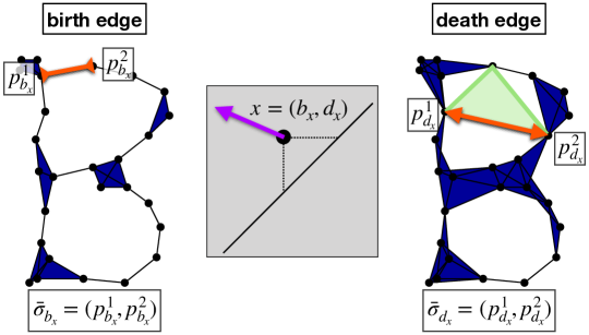
Figure 4. A visualization of how arrows (gradients) in the PD translate to arrows in the point cloud as prescribed by Lemma 2. A non-trivial generator in the PD corresponds to two edges: the one responsible for its birth (the edge that closes off some perimeter) and the one responsible for its death (the longest edge of the triangle that fills in that perimeter). Movement of the generator in the birth coordinate corresponds to extension and contraction of the birth edge, while movement in the death coordinate is the same for the death edge. By extension and contraction, we mean that the two points comprising this ‘edge’ are moved simultaneously directly toward or directly away from each other. Specifically, movement of the generator in the negative direction of one axis represents contraction, while movement in the positive direction represents extension.

3.5. Gradients for Topological Losses

We consider the gradient of the map $\alpha\mapsto d(\alpha,\beta)$ when $d$ is either the squared metric $\mathrm{FG}$ introduced in (5) or the Sinkhorn divergence for persistence diagrams $\mathrm{SFG}_{\epsilon}$ (11) based on the HUROT problem $\mathrm{FG}_{\epsilon}$ (9). When minimizing the map $\alpha\mapsto\mathrm{FG}(\alpha,\beta)$, a typical reasoning used in topological data analysis literature is the following: if we let $\zeta^{*}$ be the (generically unique) optimal partial matching between $\alpha$ and $\beta$, it is natural to define a pseudo-gradient of $\alpha\mapsto\mathrm{FG}(\alpha,\beta)$ by

(12) $$\nabla_{\alpha}\mathrm{FG}(\alpha,\beta):x\mapsto\nabla_{x}\|x-\zeta^{*}(x)\|^{2}=2(x-\zeta^{*}(x)).$$

That is, a gradient step pushes each $x$ in $\alpha$ toward its corresponding $\zeta^{*}(x)$ (whether this belongs to the support of $\beta$ or to the diagonal $\partial\Omega$). A pseudo-gradient of the map $\alpha\mapsto\mathrm{FG}(\alpha,\beta)$ defined in this way can be identified with the usual meaning of gradient for the map $(\mathbb{R}^{2})^{N}\to\mathbb{R}$ given by $(x_{1},\dots,x_{N})\mapsto\mathrm{FG}\left(\sum_{i=1}^{N}\delta_{x_{i}},\beta\right)$.

A key contribution of Leygonie et al. (2021, Section 3.2 and 3.3) was in showing that this pseudo-gradient can indeed be used in a chain rule setting with Lemma 2. Formally, gradients of maps of the form $Q\mapsto L(\mathrm{PD}(Q))$ (with $L:\mathcal{D}\to\mathbb{R}$) can be obtained as the composition of the corresponding gradient and pseudo-gradient. In particular, though the parametrization of $\alpha$ and of any gradients by the $n$-tuple $(x_{1},\dots,x_{N})$ depends on the choice of an ordering, the eventual chain rule is independent of this choice.

Building on this result, we derive the gradient of the Sinkhorn divergence for persistence diagrams that we use in our implementation. To alleviate notation, for some partial transport plan $P\in\Pi$ we will write its total mass as

$$\mathbf{M}(P)=\sum_{\begin{subarray}{c}1\leq i\leq N,\\ 1\leq j\leq M\end{subarray}}P_{ij}$$

and we let

$$\mathbf{M}_{i}(P)=\sum_{1\leq j\leq M}P_{ij}$$

(the fraction mass transported from $x_{i}$ to any of the $y_{j}$, $j=1,\dots,M$). We then introduce the barycentric map with parameter $\epsilon>0$ from $\alpha$ to $\beta$ defined on $\{x_{1},\dots,x_{N}\}$ by

$$\frac{1}{2}T^{\epsilon}_{\alpha,\beta}(x_{i})=p_{\partial\Omega}(x_{i})\left(1-\mathbf{M}_{i}(P_{\alpha,\beta}^{\epsilon})\right)+\sum_{j=1}^{M}(P^{\epsilon}_{\alpha,\beta})_{ij}\cdot y_{j},$$

where $P^{\epsilon}_{\alpha,\beta}$ is the unique optimal partial transportation plan for $\mathrm{FG}_{\epsilon}(\alpha,\beta)$. Note that the self-optimal partial transportation plan $P^{\epsilon}_{\alpha,\alpha}$ is necessarily symmetric.

Proposition 3.

Let $\alpha=\sum_{i=1}^{N}\delta_{x_{i}},\ \beta=\sum_{j=1}^{M}\delta_{y_{j}}$ be two persistence diagrams. The gradient of $\alpha\mapsto\mathrm{SFG}_{\epsilon}(\alpha,\beta)$ in the sense of (Leygonie et al., 2021) is the map defined on $\{x_{1},\dots,x_{N}\}$ by

(13) $$\nabla_{\alpha}\mathrm{SFG}_{\epsilon}(\alpha,\beta):x_{i}\mapsto T^{\epsilon}_{\alpha,\alpha}(x_{i})-T^{\epsilon}_{\alpha,\beta}(x_{i})+\epsilon K_{i}$$

with

$$K_{i}=\left[\frac{1}{2}\frac{d_{i}-b_{i}}{\mathrm{pers}(\alpha)}\left(\mathbf{M}(P^{\epsilon}_{\alpha,\beta})-\mathbf{M}(P^{\epsilon}_{\alpha,\alpha})\right)-\frac{2}{d_{i}-b_{i}}\left(\mathbf{M}_{i}(P^{\epsilon}_{\alpha,\beta})-\mathbf{M}_{i}(P^{\epsilon}_{\alpha,\alpha})\right)\right]\begin{pmatrix}-1\\ 1\end{pmatrix},$$

where $x_{i}=(b_{i},d_{i})\in\Omega$ (so that $d_{i}>b_{i}$), for $i=1,\dots,N$.

Proof.

The gradient with respect to $x_{i}$ of $\mathrm{SFG}_{\epsilon}$ is given by

$$\nabla_{x_{i}}\left[\sum_{{i^{\prime}},j}\|x_{i^{\prime}}-y_{j}\|_{2}^{2}(P^{\epsilon}_{\alpha,\beta})_{{i^{\prime}}j}+\sum_{i^{\prime}=1}^{N}\|x_{i^{\prime}}-p_{\partial\Omega}(x_{i^{\prime}})\|_{2}^{2}\left(1-\sum_{j=1}^{M}(P^{\epsilon}_{\alpha,\beta})_{{i^{\prime}}j}\right)\right]$$

$$-\frac{1}{2} \nabla_{x_{i}}\left[\sum_{{i^{\prime}}j}\|x_{i^{\prime}}-x_{j}\|_{2}^{2}(P^{\epsilon}_{\alpha,\alpha})_{i^{\prime}j}+\sum_{i^{\prime}}\|x_{i^{\prime}}-p_{\partial\Omega}(x_{i^{\prime}})\|_{2}^{2}\left(1-\sum_{j=1}^{M}(P^{\epsilon}_{\alpha,\beta})_{{i^{\prime}}j}\right)\right]$$

$$+ \epsilon\nabla_{x_{i}}\varphi(x_{1},\dots,x_{N}),$$

where

$$\varphi(x)=\frac{1}{2}\left(\mathrm{KL}\left(P^{\epsilon}_{\alpha,\beta}\bigg{|}\frac{\mathbf{a}\mathbf{b}^{T}}{\mathrm{pers}(\alpha)}\right)+\mathrm{KL}\left(P^{\epsilon}_{\alpha,\beta}\bigg{|}\frac{\mathbf{a}\mathbf{b}^{T}}{\mathrm{pers}(\beta)}\right)\right)-\frac{1}{2}\mathrm{KL}\left(P^{\epsilon}_{\alpha,\alpha}\bigg{|}\frac{\mathbf{a}\mathbf{a}^{T}}{\mathrm{pers}(\alpha)}\right)$$

accounts for the entropic regularization terms. Note that $\varphi$ depends on $x$ since the column vector $\mathbf{a}$ accounts for the squared distance between the points in $\mathrm{supp}(\alpha)$ and their projection on the diagonal $\partial\Omega$.

Computing the gradient of the first term yields

$$\nabla_{x_{i}}\left[\sum_{i^{\prime},j}\|x_{i^{\prime}}-y_{j}\|_{2}^{2}(P^{\epsilon}_{\alpha,\beta})_{{i^{\prime}}j}+\sum_{i^{\prime}=1}^{N}\|x_{i^{\prime}}-p_{\partial\Omega}(x_{i^{\prime}})\|_{2}^{2}\left(1-\sum_{j=1}^{m}(P^{\epsilon}_{\alpha,\beta})_{{i^{\prime}}j}\right)\right]$$

$$= 2\sum_{j=1}^{M}(x_{i}-y_{j})(P^{\epsilon}_{\alpha,\beta})_{ij}+2(x_{i}-p_{\partial\Omega}(x_{i}))\left(1-\sum_{j=1}^{M}(P^{\epsilon}_{\alpha,\beta})_{ij}\right)$$

$$= 2x_{i}-2\left(\sum_{j=1}^{M}y_{j}(P^{\epsilon}_{\alpha,\beta})_{ij}+p_{\partial\Omega}(x_{i})\left(1-\sum_{j=1}^{M}(P^{\epsilon}_{\alpha,\beta})_{ij}\right)\right)$$

$$= 2x_{i}-T^{\epsilon}_{\alpha,\beta}(x_{i}).$$

For the second term, using the symmetry of $P^{\epsilon}_{\alpha,\alpha}$ and the above calculation, we have

$$\frac{1}{2}\nabla_{x_{i}}\left[\sum_{i^{\prime},j}\|x_{i^{\prime}}-x_{j}\|_{2}^{2}(P^{\epsilon}_{\alpha,\alpha})_{{i^{\prime}}j}+\sum_{i^{\prime}=1}^{N}\|x_{i^{\prime}}-p_{\partial\Omega}(x_{i^{\prime}})\|_{2}^{2}\left(1-\sum_{j=1}^{M}(P^{\epsilon}_{\alpha,\alpha})_{{i^{\prime}}j}\right)\right]$$

$$= 2x_{i}-T^{\epsilon}_{\alpha,\alpha}(x_{i}).$$

The gradient of $\varphi$ is obtained by expanding the factors in the different $\mathrm{KL}$ terms and observing that $\nabla_{x_{i}}\|x_{i}-p_{\partial\Omega}(x_{i})\|^{2}=(d_{i}-b_{i})\begin{pmatrix}-1\\ 1\end{pmatrix}$, resulting in

$$\frac{1}{2}\nabla_{x_{i}}\log(\mathrm{pers}(\alpha))\sum_{i^{\prime}j}(P^{\epsilon}_{\alpha,\beta})_{i^{\prime}j}-\nabla_{x_{i}}\sum_{i^{\prime}j}(P^{\epsilon}_{\alpha,\beta})_{i^{\prime}j}\log(\|x_{j}-p_{\partial\Omega}(x_{j})\|^{2})$$

$$-\frac{1}{2}\nabla_{x_{i}}\log(\mathrm{pers}(\alpha))\sum_{jk}(P^{\epsilon}_{\alpha,\alpha})_{jk}+\nabla_{x_{i}}\sum_{jk}(P^{\epsilon}_{\alpha,\alpha})_{jk}\log(\|x_{j}-p_{\partial\Omega}(x_{j})\|^{2})$$

$$+\nabla_{x_{i}}\frac{1}{2}\mathrm{pers}(\alpha)-\nabla_{x_{i}}\frac{1}{2}\mathrm{pers}(\alpha))$$

$$= \left[\frac{1}{2}\frac{d_{i}-b_{i}}{\mathrm{pers}(\alpha)}\left(\mathbf{M}(P^{\epsilon}_{\alpha,\beta})-\mathbf{M}(P^{\epsilon}_{\alpha,\alpha})\right)-\frac{2}{d_{i}-b_{i}}\left(\mathbf{M}_{i}(P^{\epsilon}_{\alpha,\beta})-\mathbf{M}_{i}(P^{\epsilon}_{\alpha,\alpha})\right)\right]\begin{pmatrix}-1\\ 1\end{pmatrix}.$$

Putting these terms together completes the proof. ∎

Remark 4.

Interestingly, the term $T^{\epsilon}_{\alpha,\beta}-T^{\epsilon}_{\alpha,\alpha}$ appearing in our gradient can be related to (Carlier et al., 2022, Section 4.2), where it is shown that this quantity represents the tangent vector field for the gradient flow of the Sinkhorn divergence between probability measures (instead of persistence diagrams). Because of the particular role played by the diagonal in our problem, we have the additional term $\epsilon K_{i}$ which acts orthogonally to the diagonal to account for our distance-weighted entropic term. In particular, when we take the limit as $\epsilon\to 0$, since $T^{\epsilon}_{\alpha,\beta}\to P_{\alpha,\beta}$ and $T^{\epsilon}_{\alpha,\alpha}\to\mathrm{id}$, we expect to retrieve the descent direction $P_{\alpha,\beta}-\mathrm{id}$ which exactly describes the pseudo-gradient (12) and is the geodesic between $\alpha$ and $\beta$ for the usual $\mathrm{FG}(\cdot,\cdot)^{\frac{1}{2}}$ metric (Turner et al., 2014). This is analogous to the displacement interpolation proposed by McCann in OT literature (McCann, 1997).

4. Topological Node2vec

In order to utilize topological information in Node2vec, we need to be able to extract a persistence diagram from a graph. Recall from Section 3.1 that the Vietoris-Rips construction of the persistence diagram relies only on pairwise distances between points, for which we can easily make an analog involving the weights of edges in a graph $G=(V,E,w)$. Namely, the persistence diagram $\mathrm{PD}(G)$ of a graph $G$ is the one extracted from the Vietoris-Rips filtration $\{\mathrm{VR}_{\rho}\}$ where each edge $(u,v)\in V\times V$ is inserted at time

$$\frac{1}{(w(u,v)+\gamma)^{\nu}}$$

for $\nu,\gamma>0$ with $\gamma$ very small ($1/\gamma^{\nu}$ becoming the distance between points connected by zero-weight edges in the graph). This ensures that vertices $u,v$ connected by a strong (resp. weak) edge in the graph $w(u,v)$ are regarded as close (resp. far) in the view of the Vietoris-Rips filtration.

Definition 5.

For a Node2vec model with input graph $G$ and parameters $\Theta=(W_{1},W_{2})$, we define the topological loss term

(14) $$L_{1}(G,\Theta)=\mathrm{SFG}_{\epsilon}(\mathrm{PD}(\mathrm{Emb}(\Theta)),\mathrm{PD}(G)).$$

Recall from Definition 1 that $\mathrm{Emb}(\Theta)$ is the matrix $W_{1}$ with its rows viewed as Euclidean points. It follows immediately that the gradient of $L_{1}$ with respect to any coordinate of $W_{2}$ is zero.

We are now ready to state the gradient of the topological loss function $L_{1}(\Theta,G)$ with respect to $\Theta$, or, as clarified above, with respect to the points $p$ in the current embedding $\mathrm{Emb}(\Theta)$.

Theorem 1 (Gradient of Topological Loss Term).

Let $\alpha=\mathrm{PD}(\mathrm{Emb}(\Theta))$ and $\beta\subset\Omega$. Let $\zeta_{\epsilon}$ be the gradient of $\alpha\mapsto\mathrm{SFG}_{\epsilon}(\alpha,\beta)$ as provided by (13). Let $p\in\mathrm{Emb}(\Theta)$. We have

$$\frac{\partial L_{1}}{\partial p}=\sum_{x\in\mathrm{PD}(\mathrm{Emb}(\Theta))}\zeta_{\epsilon}(x)\cdot\dfrac{\partial x}{\partial p},$$

where the partial derivative $\dfrac{\partial x}{\partial p}$ is provided by Lemma 2.

Proof.

From the chain rule of (Leygonie et al., 2021) (see Section 3.5) and Equation 13 it follows that

$$\dfrac{\partial L_{1}}{\partial p} =\sum_{x\in\mathrm{PD}(\mathrm{Emb}(\Theta))}\dfrac{\partial\mathrm{SFG}_{\epsilon}}{\partial x}\cdot\dfrac{\partial x}{\partial p}$$

$$=\sum_{x\in\mathrm{PD}(\mathrm{Emb}(\Theta))}\zeta_{\epsilon}(x)\cdot\dfrac{\partial x}{\partial p}.$$

∎

We can now train Node2vec using a loss

$$L(\Theta)=\lambda_{0}L_{0}(T,\Theta)+\lambda_{1}L_{1}(G,\Theta)$$

for some parameters $\lambda_{0},\lambda_{1}\geq 0$, using a standard gradient descent framework with a learning rate $\eta>0$. Let $\Theta(k)$ denote the parameters after $k\in\mathbb{Z}_{\geq 0}$ steps of gradient descent updates. Then the next epoch’s parameters are given by

(15) $$\Theta(k+1):=\Theta(k)-\eta\left(\lambda_{0}\nabla_{\Theta(k)}L_{0}(T(k),\Theta(k))+\lambda_{1}\nabla_{\Theta(k)}L_{1}(G,\Theta(k))\right)$$

with individual gradients given by Proposition 1 and Theorem 1. We summarize this in Algorithm 2.

Algorithm 2 Topological Node2vec algorithm

a weighted graph $G=(V,E,w)$, learning rates $\eta,\lambda_{0},\lambda_{1}$, embedding dimension $m$, neighborhood parameters $(l,r,p,q)$, entropic regularization parameter $\epsilon>0$;

$\mathbb{P}\subset\mathbb{R}^{m}$ with $|\mathbb{P}|=|V|$

• initialize the parameter matrices $\Theta(0)$; let $k=0$;

• compute the persistence diagram $\mathrm{PD}(G)$

while not converged do

     • compute the persistence diagram $\mathrm{PD}(\mathrm{Emb}(\Theta(k)))$

     • for each node $v\in V$, generate the current neighborhood vector $C_{v}$ and the training neighborhood vector $T_{v}$; let $C(k)=\{C_{v}(k)\}_{v\in V}$ and $T(k):=\{T_{v}(k)\}_{v\in V}$

     • update $\Theta(k+1)$ using (15)

     • $k\mathrel{+}=1$

end while

5. Numerical Experiments

In this section, we elaborate on two synthetic experiments designed to demonstrate what we gain over the base Node2vec model by including our topological loss function (14).

Our code is publicly available at this repository. Its implementation provides both CPU and GPU backend. The CPU-backend relies on Gudhi (Maria et al., 2014), while the GPU-backend is based on a fork of Ripser++ (Bauer, 2021; Zhang et al., 2020b) where we adapted the code in order to access the correspondence between a generator $x$ in the PD and the points in the point cloud responsible for the birth edge and death edge. For an in-depth examination of all the hyperparameters of this network (both those related to original Node2vec as well as our topological additions), please see the readme file and examples notebook in the repository.

5.1. Experiment: $S^{1}$ Made of 8 Smaller $S^{1}$s

Figure 5. Euclidean data for the synthetic experiment, from which we derive a weighted adjacency matrix to input into (Topological) Node2vec. This data set demonstrates overt topological features on two scales: the eight smaller cycles and the larger emergent cycle formed by their arrangement.

We look at a dataset consisting of 8 circles each with 16 points arranged radially in a larger circle, seen in Figure 5. While the points and the sampled circles themselves are distributed uniformly, each point is wiggled by some small random noise, ensuring that the input data satisfies Vietoris-Rips general position (which is guaranteed if all pairwise distances are unique).

Node2vec neighborhood generation. We first demonstrate that, as shown in Figure 6, for this data set it is best to forego the random neighborhood generation of Node2vec and simply use as neighborhoods the columns of the adjacency matrix corresponding to each vertex. (See Remark 1.)

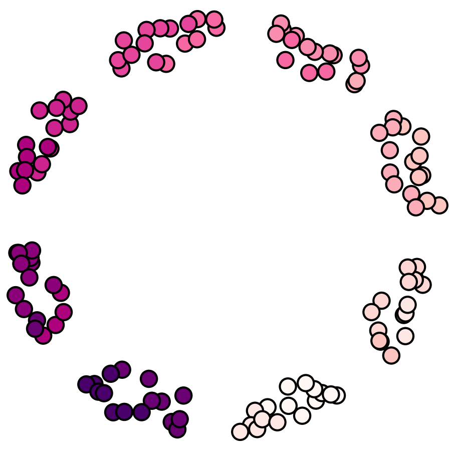
(a) $l=1,r=8$

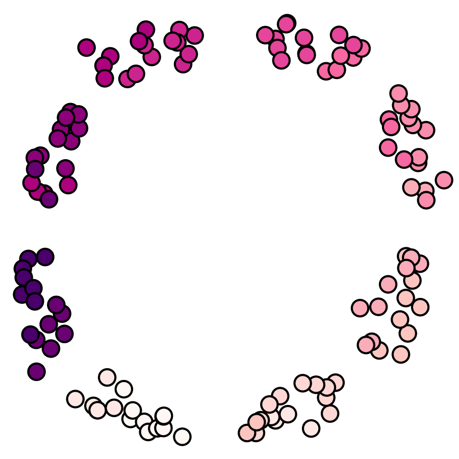
(b) $l=2,r=4$

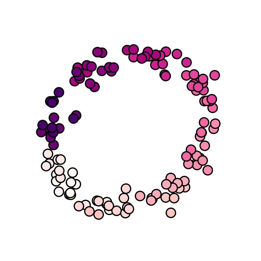
(c) linear interpolation from $l=1,r=8$ to $l=8,r=1$

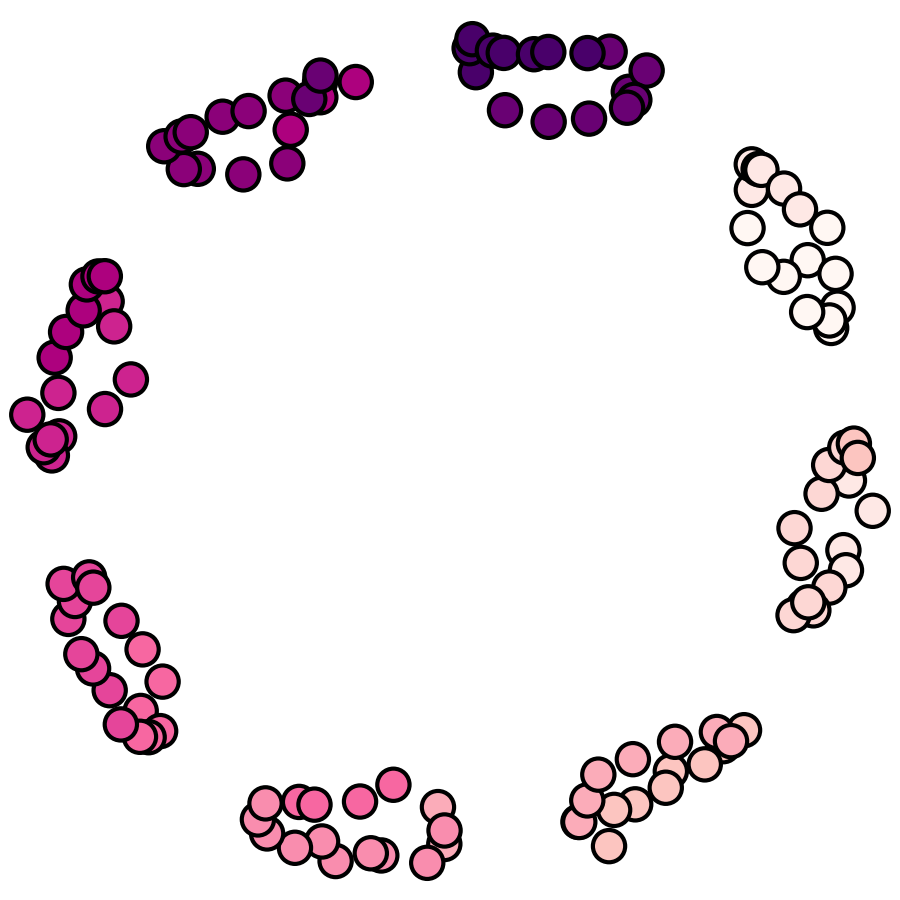
(d) $l=1,r=16$

(e) $l=1,r=\infty$, as in Remark 1

Figure 6. Various non-topological Node2vec embeddings of the point cloud in Figure 5 (specifically the reciprocal of its pairwise distance matrix) trained with different neighborhood parameters. Even in the best case, original Node2vec dramatically erases topological information. (a – d) We see that $l=1$ and $r$ large give the best results. (e) This embedding was done using full-column vectors for neighborhood information.

Minibatches are important outside of computation time. Upon introduction of the topological loss function (14), we immediately encounter a novel problem. When identifying some topological feature in the embedding and matching it to a smaller feature in the original data (something that is closer to the diagonal), the gradient update of the topological loss function (14) expands the birth edge and shrinks the death edge of the feature. (Recall Figure 4.) However, the points that dictated the birth and death values of this feature are now all but guaranteed to be the same determining points in the next step of the network, causing a repeat of the same movement on the same points, leaving the rest of the data set untouched and the embedding progressively distorted. Taking properly sized minibatches (subsampling the data at each step of the network) can completely remove this problem, as the points determining the birth or death of such a generator are likely to change from one step to the next. Figure 7 demonstrates this in detail.

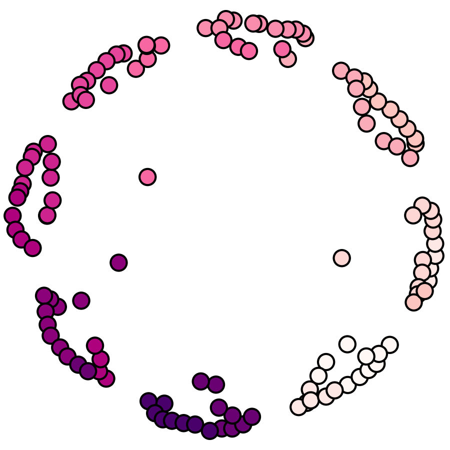
(a) No minibatching: 100% of data used at every epoch.

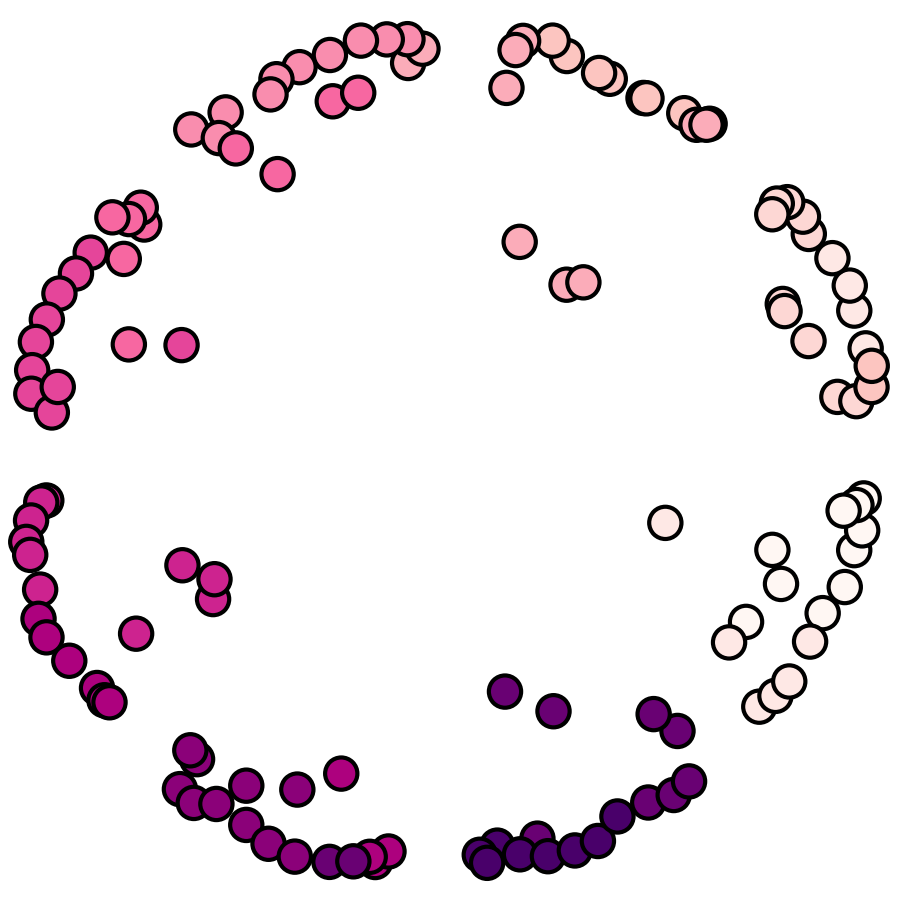
(b) Minibatches of 75% of data.

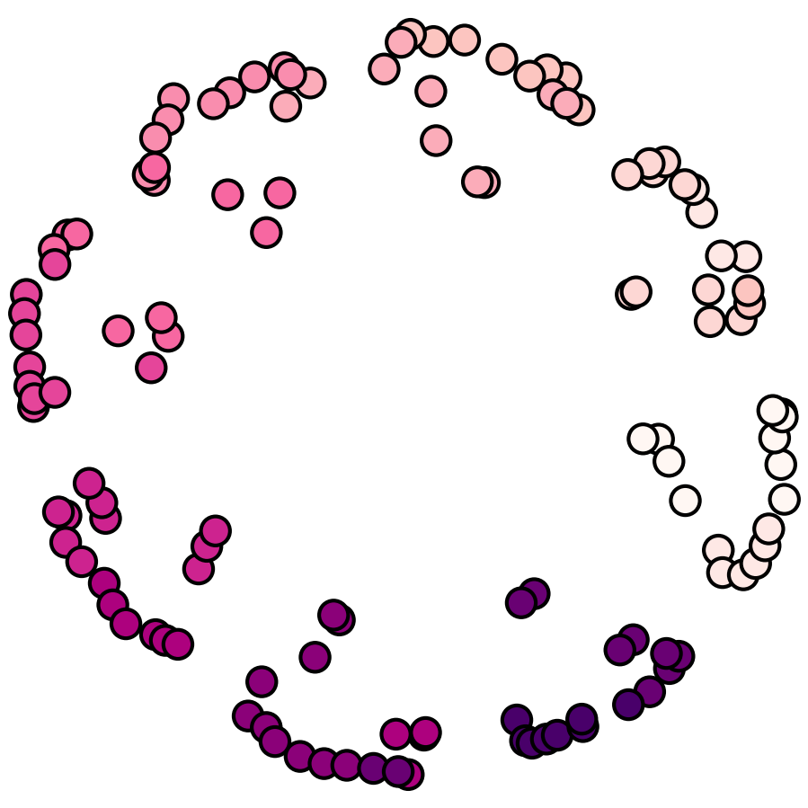
(c) Minibatches of 50% of data.

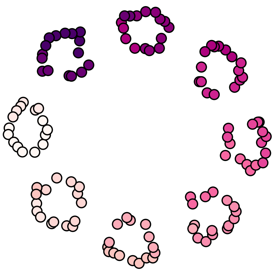
(d) Minibatches of 25% of data.

(e) Minibatches graded from 25% of data at the beginning of the embedding process to 100% at the end.

Figure 7. Topological Node2vec embeddings demonstrating the topological loss function’s interaction with minibatch size. (a – d) As minibatches decrease in size, the inward distortion of the points that provide the death value of the inner topological feature also decreases. (e) Testing for potential improvement, we performed another embedding beginning with 25% minibatches and then linearly increasing to 100 % as the model continued to train. All other parameters are fixed across these five experiments.

Results. Comparing the best results from original Node2vec in Figure 6 (e) and the best results from Topological Node2vec in Figure 7 (e), we can starkly see the information loss in base Node2vec as well as our recovery of it via the topological loss function (14).

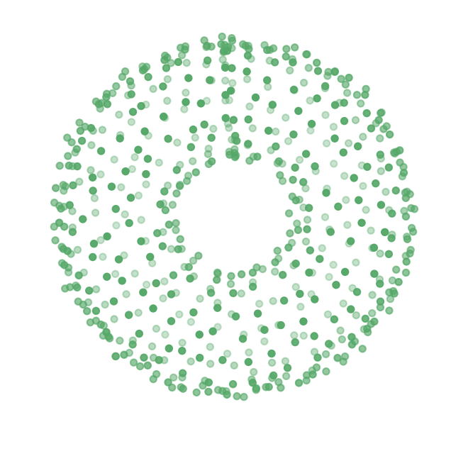
(a)

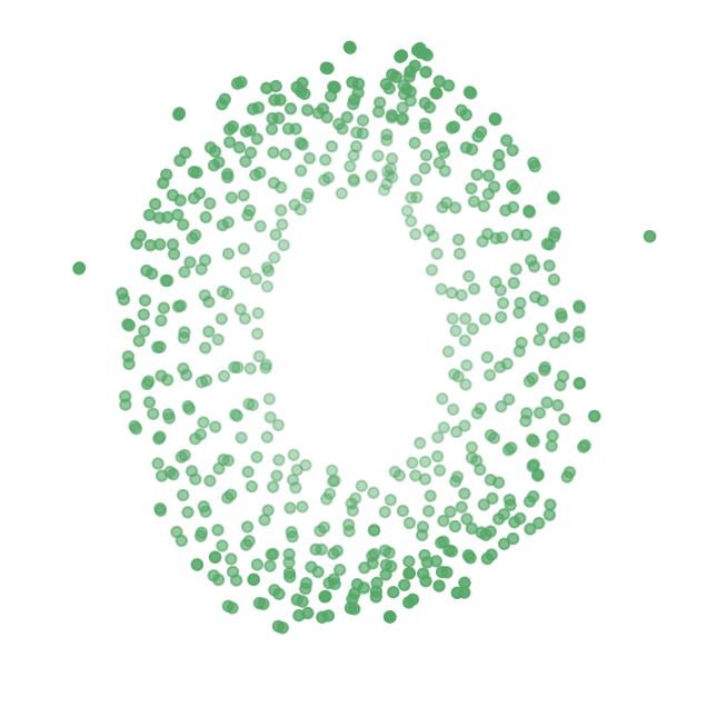
(b)

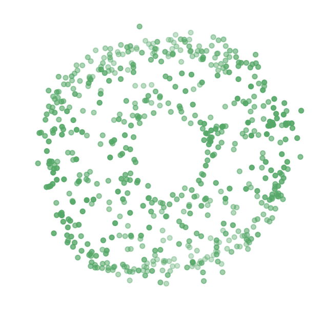
(c)

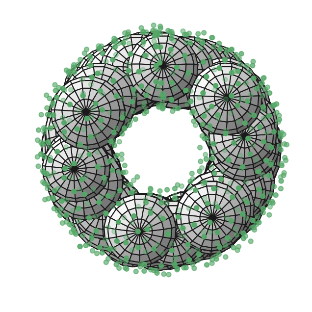
(d)

(e)

(f)

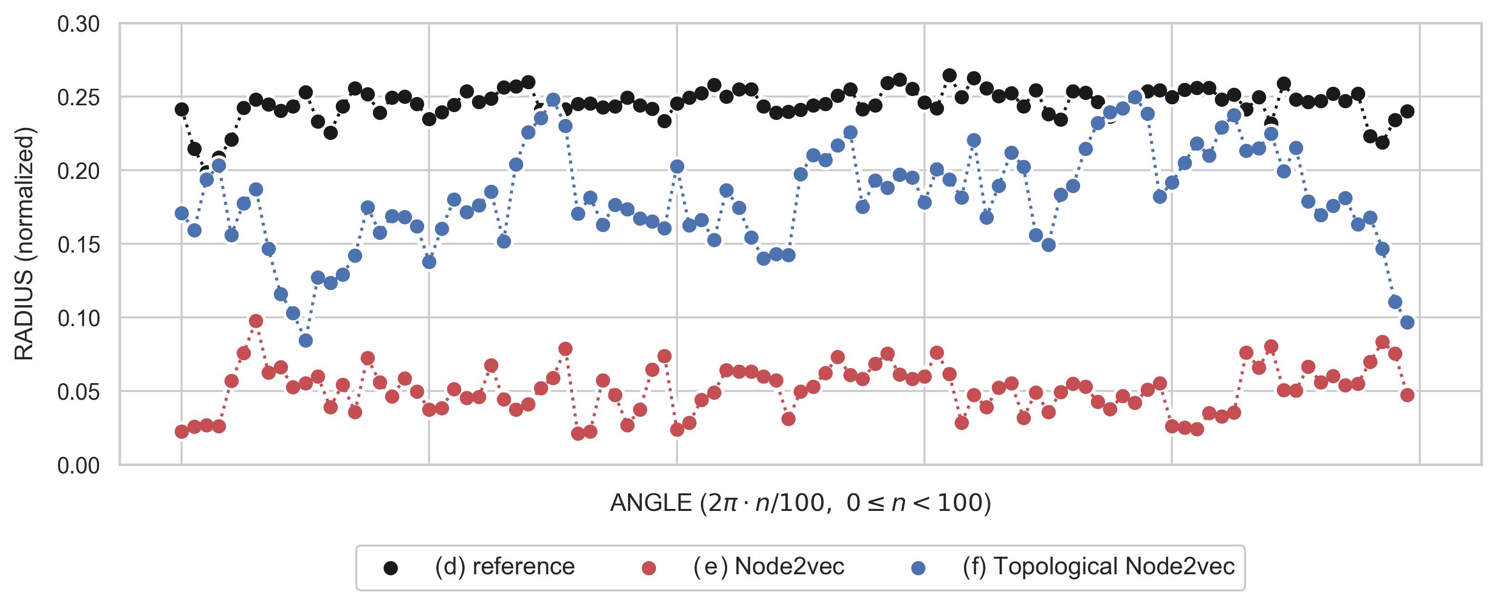
(g)

Figure 8. 3D render of various point clouds with largest inscribable spheres drawn inside. (a,d) Synthetic data created for this experiment. (b,e) Best embedding proposed by Node2vec over various hyper-parameters. (c,f) Best embedding proposed by Topological Node2vec over extensive space of hyper-parameters. (g) A plot of the radii of all largest inscribable spheres drawn inside the preceding tori. In these examples, one hundred evenly distributed angles are taken, and all radii have been normalized by the final diameter of their corresponding embedding.

5.2. Experiment: Torus

We sample a torus by arranging points uniformly over the surface. (These are not uniformly sampled from a distribution, but rather a constructed covering. See the demonstration notebook in the repository for the precise details.) Once again, in order to ensure Vietoris-Rips general position, we perturb all points by a small random vector.

The smooth torus has two independent one-dimensional topological features, representing one horizontal loop around the torus and one vertical one. The torus also has a single two-dimensional feature that represents the hollow interior. We benefit here from a very small minibatch size, eventually settling on 6.25% of the full data set, constant across all epochs.

Visualization. To visualize our embedded tori, we project the results into the first two principal components with the third principal component corresponding to distance from the viewer.

Visualizing the reconstruction of the two-dimensional topological feature (the hollow tube) is vital to judging the success of any torus embedding. To draw the ‘largest’ inscribable spheres as in Figure 8, in increments of very small angles we take rectangular slices of the torus widened from the ray that starts at the torus’ center and extends in the direction of the current angle. Averaging all points on this rectangle, we obtain a central point $c$. We then inscribe the largest possible sphere at that center.

Results. We note the dramatic loss of topology in Node2vec and equally dramatic recovery of such features with the inclusion of the topological loss function (14) demonstrated in Figure 8.

6. Discussion

The most obvious limiting factor for applying this model is the computation time of acquiring the persistence diagram of the proposed embedding at every epoch. Fortunately, in our synthetic examples, it is almost always the case that the best embeddings come out of very small minibatch sizes, which also result in dramatically reduced computation times. As PD computation becomes further optimized, the model will benefit tremendously.

Since the generating point cloud (and thus the resulting persistence diagram) is only very marginally altered from one epoch to the next, this project seems potentially suitable for application of the work in (Cohen-Steiner et al., 2006) which may dramatically reduce computation time after generating the initial persistence diagram. However, this conflicts (at least at first glance) with subsampling minibatches at every epoch, which causes us to have largely unrelated PDs from one epoch to the next.

Part of the motivation for this project is the need for improved analysis of chromatin conformation capture data obtained from methods such as Hi-C and Pore-C (Ulahannan et al., 2019). These data represent the frequency of all two-contacts (Hi-C) or multi-contacts (Pore-C) among DNA segments and can be considered as graphs (Hi-C) or hypergraphs (Pore-C). It is biologically known that chromatin conformation is dynamically deformed and forms first-order and second-order topological structures to regulate gene expression in the cell differentiation process. Reconstructing three-dimensional topological structures of DNA from these data is a crucial point of current cell research, and can be regarded as a problem of graph (or hypergraph) embeddings. Our demonstrations in this document make it clear that conventional data analysis using Node2vec-based methods are unlikely to capture chromatin conformation precisely due to the eradication of topology, and Topological Node2vec hopes to resolve this. The validation of Topological Node2vec as applied to epigenome data science is the primary concern of our future work.

Acknowledgments and Disclosure of Funding

This work was sponsored by JSPS Grant-in-Aid for Transformative Research Areas (A) (no. 22H05107 to Y. Hiraoka), JST MIRAI Program Grant (no. 22682401 to Y. Hiraoka), JST PRESTO (no. JPMJPR2021 to Y. Imoto), AAP CNRS INS2I 2022 (to T. Lacombe), and JSPS Grant-in-Aid for Early-Career Scientists (no. 21K13822, to T. Yachimura), ASHBi Fusion Research Program (to Y. Imoto and K. Meehan).

Appendix A Delayed Proofs

Proof of Proposition 1.

Let $v=v_{i}$, $1\leq j\leq m$, and $1\leq l\leq n$.

$$\phantom{=}\frac{\partial H(T_{v},C_{v})}{\partial W_{1}(l,j)}=-\frac{\partial\sum_{1\leq a\leq n}T_{v}(a)u_{v}(a)}{\partial W_{1}(l,j)}+\frac{\partial\log\sum_{1\leq a\leq n}e^{u_{v}(a)}}{\partial W_{1}(l,j)}$$

$$=-\sum_{1\leq a\leq n}T_{v}(a)\sum_{1\leq b\leq m}\dfrac{\partial W_{1}(i,b)W_{2}(b,a)}{\partial W_{1}(l,j)}+\sum_{1\leq a\leq n}e^{u_{v}(a)}\frac{\partial u_{v}(a)}{\partial W_{1}(l,j)}\cdot\dfrac{1}{\sum_{1\leq a\leq n}e^{u_{v}(a)}}$$

$$=-\delta_{il}\sum_{1\leq a\leq n}(T_{v}(a)W_{2}(j,a)+W_{2}(j,a)C_{v}(a))$$

$$=\delta_{il}\sum_{1\leq a\leq n}W_{2}(j,a)(C_{v}(a)-T_{v}(a)).$$

Next,

$$\phantom{=}\frac{\partial H(T_{v},C_{v})}{\partial W_{2}(j,l)}=\frac{\partial(-\sum_{1\leq a\leq n}T_{v}(a)u_{v}(a)+\log\sum_{1\leq a\leq n}e^{u_{v}(a)})}{\partial W_{2}(j,l)}$$

$$=-\frac{\partial\sum_{1\leq a\leq n}T_{v}(a)u_{v}(a)}{\partial W_{2}(j,l)}+\frac{\partial\log\sum_{1\leq a\leq n}e^{u_{v}(a)}}{\partial W_{2}(j,l)}$$

$$=-\sum_{1\leq a\leq n}T_{v}(a)\frac{\partial u_{v}(a)}{\partial W_{2}(j,l)}+\sum_{1\leq a\leq n}\frac{\partial e^{u_{v}(a)}}{\partial W_{2}(j,l)}\cdot\dfrac{1}{\sum_{1\leq a\leq n}e^{u_{v}(a)}}$$

$$=-\sum_{1\leq a\leq n}T_{v}(a)\sum_{1\leq b\leq m}\dfrac{\partial W_{1}(i,b)W_{2}(b,a)}{\partial W_{2}(j,l)}+\sum_{1\leq a\leq n}e^{u_{v}(a)}\frac{\partial u_{v}(a)}{\partial W_{2}(j,l)}\cdot\dfrac{1}{\sum_{1\leq a\leq n}e^{u_{v}(a)}}$$

$$=-T_{v}(l)W_{1}(i,j)+W_{1}(i,j)\cdot\dfrac{e^{u_{v}(l)}}{\sum_{1\leq a\leq n}e^{u_{v}(a)}}$$

$$=W_{1}(i,j)(C_{v}(l)-T_{v}(l)).$$

That is, the gradient of $L_{0}(T_{v},C_{v})$ with respect to $W_{1}$ is non-zero only when taking partials with respect to the $i^{\text{th}}$ row of $W_{1}$ (recall $v=v_{i}$). ∎

References

- Altschuler et al. (2017) J. Altschuler, J. Niles-Weed, and P. Rigollet. Near-linear time approximation algorithms for optimal transport via sinkhorn iteration. Advances in neural information processing systems, 30, 2017.
- Bauer (2021) U. Bauer. Ripser: efficient computation of vietoris–rips persistence barcodes. Journal of Applied and Computational Topology, 5(3):391–423, 2021.
- Benamou et al. (2015) J.-D. Benamou, G. Carlier, M. Cuturi, L. Nenna, and G. Peyré. Iterative bregman projections for regularized transportation problems. SIAM Journal on Scientific Computing, 37(2):A1111–A1138, 2015.
- Bojchevski and Günnemann (2018) A. Bojchevski and S. Günnemann. Deep gaussian embedding of graphs: Unsupervised inductive learning via ranking, 2018.
- Brüel-Gabrielsson et al. (2020) R. Brüel-Gabrielsson, V. Ganapathi-Subramanian, P. Skraba, and L. J. Guibas. Topology-aware surface reconstruction for point clouds. In Computer Graphics Forum, volume 39, pages 197–207. Wiley Online Library, 2020.
- Cao et al. (2015) S. Cao, W. Lu, and Q. Xu. Grarep: Learning graph representations with global structural information. In Proceedings of the 24th ACM International on Conference on Information and Knowledge Management, CIKM ’15, page 891–900, New York, NY, USA, 2015. Association for Computing Machinery. ISBN 9781450337946. doi: 10.1145/2806416.2806512. URL https://doi.org/10.1145/2806416.2806512.
- Cao and Monod (2022) Y. Cao and A. Monod. Approximating persistent homology for large datasets. arXiv preprint arXiv:2204.09155, 2022.
- Carlier et al. (2022) G. Carlier, L. Chizat, and M. Laborde. Lipschitz continuity of the schrödinger map in entropic optimal transport. arXiv preprint arXiv:2210.00225, 2022.
- Carriere et al. (2021) M. Carriere, F. Chazal, M. Glisse, Y. Ike, H. Kannan, and Y. Umeda. Optimizing persistent homology based functions. In M. Meila and T. Zhang, editors, Proceedings of the 38th International Conference on Machine Learning, volume 139 of Proceedings of Machine Learning Research, pages 1294–1303. PMLR, 18–24 Jul 2021. URL https://proceedings.mlr.press/v139/carriere21a.html.
- Chazal et al. (2016) F. Chazal, V. De Silva, M. Glisse, and S. Oudot. The structure and stability of persistence modules, volume 10. Springer, 2016.
- Chen et al. (2019) C. Chen, X. Ni, Q. Bai, and Y. Wang. A topological regularizer for classifiers via persistent homology. In The 22nd International Conference on Artificial Intelligence and Statistics, pages 2573–2582. PMLR, 2019.
- Cohen-Steiner et al. (2005) D. Cohen-Steiner, H. Edelsbrunner, and J. Harer. Stability of persistence diagrams. In Proceedings of the twenty-first annual symposium on Computational geometry, pages 263–271, 2005.
- Cohen-Steiner et al. (2006) D. Cohen-Steiner, H. Edelsbrunner, and D. Morozov. Vines and vineyards by updating persistence in linear time. In Proceedings of the Twenty-Second Annual Symposium on Computational Geometry, SCG ’06, page 119–126, New York, NY, USA, 2006. Association for Computing Machinery. ISBN 1595933409. doi: 10.1145/1137856.1137877. URL https://doi.org/10.1145/1137856.1137877.
- Cohen-Steiner et al. (2010) D. Cohen-Steiner, H. Edelsbrunner, J. Harer, and Y. Mileyko. Lipschitz functions have l p-stable persistence. Foundations of computational mathematics, 10(2):127–139, 2010.
- Cui et al. (2018) P. Cui, X. Wang, J. Pei, and W. Zhu. A survey on network embedding. IEEE transactions on knowledge and data engineering, 31(5):833–852, 2018.
- Cuturi (2013) M. Cuturi. Sinkhorn distances: Lightspeed computation of optimal transport. In C. Burges, L. Bottou, M. Welling, Z. Ghahramani, and K. Weinberger, editors, Advances in Neural Information Processing Systems, volume 26. Curran Associates, Inc., 2013. URL https://proceedings.neurips.cc/paper/2013/file/af21d0c97db2e27e13572cbf59eb343d-Paper.pdf.
- Divol and Lacombe (2021a) V. Divol and T. Lacombe. Understanding the topology and the geometry of the space of persistence diagrams via optimal partial transport. Journal of Applied and Computational Topology, 5, 3 2021a. ISSN 23671734. doi: 10.1007/s41468-020-00061-z.
- Divol and Lacombe (2021b) V. Divol and T. Lacombe. Estimation and quantization of expected persistence diagrams. In International Conference on Machine Learning, pages 2760–2770. PMLR, 2021b.
- Dvurechensky et al. (2018) P. Dvurechensky, A. Gasnikov, and A. Kroshnin. Computational optimal transport: Complexity by accelerated gradient descent is better than by sinkhorn’s algorithm. In International conference on machine learning, pages 1367–1376. PMLR, 2018.
- Edelsbrunner and Harer (2022) H. Edelsbrunner and J. L. Harer. Computational topology: an introduction. American Mathematical Society, 2022.
- Edelsbrunner et al. (2000) H. Edelsbrunner, D. Letscher, and A. Zomorodian. Topological persistence and simplification. In Proceedings 41st Annual Symposium on Foundations of Computer Science, pages 454–463, 2000. doi: 10.1109/SFCS.2000.892133.
- Feydy et al. (2019) J. Feydy, T. Séjourné, F.-X. Vialard, S.-i. Amari, A. Trouvé, and G. Peyré. Interpolating between optimal transport and mmd using sinkhorn divergences. In The 22nd International Conference on Artificial Intelligence and Statistics, pages 2681–2690. PMLR, 2019.
- Figalli and Gigli (2010) A. Figalli and N. Gigli. A new transportation distance between non-negative measures, with applications to gradients flows with dirichlet boundary conditions. Journal des Mathematiques Pures et Appliquees, 94:107–130, 8 2010. ISSN 00217824. doi: 10.1016/j.matpur.2009.11.005.
- Gabrielsson et al. (2020) R. B. Gabrielsson, B. J. Nelson, A. Dwaraknath, and P. Skraba. A topology layer for machine learning. In S. Chiappa and R. Calandra, editors, Proceedings of the Twenty Third International Conference on Artificial Intelligence and Statistics, volume 108 of Proceedings of Machine Learning Research, pages 1553–1563. PMLR, 26–28 Aug 2020. URL https://proceedings.mlr.press/v108/gabrielsson20a.html.
- Gameiro et al. (2016) M. Gameiro, Y. Hiraoka, and I. Obayashi. Continuation of point clouds via persistence diagrams. Physica D: Nonlinear Phenomena, 334:118–132, 2016. ISSN 0167-2789. doi: https://doi.org/10.1016/j.physd.2015.11.011. URL https://www.sciencedirect.com/science/article/pii/S0167278915002626. Topology in Dynamics, Differential Equations, and Data.
- Genevay et al. (2018) A. Genevay, G. Peyré, and M. Cuturi. Learning generative models with sinkhorn divergences. In International Conference on Artificial Intelligence and Statistics, pages 1608–1617. PMLR, 2018.
- Grover and Leskovec (2016) A. Grover and J. Leskovec. node2vec: Scalable feature learning for networks. In Proceedings of the 22nd ACM SIGKDD international conference on Knowledge discovery and data mining, pages 855–864, 2016.
- Hensel et al. (2021) F. Hensel, M. Moor, and B. Rieck. A survey of topological machine learning methods. Frontiers in Artificial Intelligence, 4, 2021. ISSN 2624-8212. doi: 10.3389/frai.2021.681108. URL https://www.frontiersin.org/article/10.3389/frai.2021.681108.
- Hu et al. (2019) X. Hu, F. Li, D. Samaras, and C. Chen. Topology-preserving deep image segmentation. Advances in neural information processing systems, 32, 2019.
- Janati et al. (2020) H. Janati, M. Cuturi, and A. Gramfort. Debiased sinkhorn barycenters. In International Conference on Machine Learning, pages 4692–4701. PMLR, 2020.
- Kantorovich (1942) L. V. Kantorovich. On the translocation of masses. Journal of mathematical sciences, 133(4):1381–1382, 1942.
- Lacombe (2023) T. Lacombe. An homogeneous unbalanced regularized optimal transport model with applications to optimal transport with boundary. In International Conference on Artificial Intelligence and Statistics, pages 7311–7330. PMLR, 2023.
- Lacombe et al. (2018) T. Lacombe, M. Cuturi, and S. Oudot. Large scale computation of means and clusters for persistence diagrams using optimal transport. In S. Bengio, H. Wallach, H. Larochelle, K. Grauman, N. Cesa-Bianchi, and R. Garnett, editors, Advances in Neural Information Processing Systems, volume 31, , 2018. Curran Associates, Inc. URL https://proceedings.neurips.cc/paper/2018/file/b58f7d184743106a8a66028b7a28937c-Paper.pdf.
- Leygonie et al. (2021) J. Leygonie, S. Oudot, and U. Tillmann. A framework for differential calculus on persistence barcodes. Foundations of Computational Mathematics, pages 1–63, 2021.
- Leygonie et al. (2023) J. Leygonie, M. Carrière, T. Lacombe, and S. Oudot. A gradient sampling algorithm for stratified maps with applications to topological data analysis. Mathematical Programming, pages 1–41, 2023.
- Maria et al. (2014) C. Maria, J.-D. Boissonnat, M. Glisse, and M. Yvinec. The gudhi library: Simplicial complexes and persistent homology. In Mathematical Software–ICMS 2014: 4th International Congress, Seoul, South Korea, August 5-9, 2014. Proceedings 4, pages 167–174. Springer, 2014.
- McCann (1997) R. J. McCann. A convexity principle for interacting gases. Advances in mathematics, 128(1):153–179, 1997.
- Mikolov et al. (2013) T. Mikolov, K. Chen, G. Corrado, and J. Dean. Efficient estimation of word representations in vector space, 2013. URL https://arxiv.org/abs/1301.3781.
- Mileyko et al. (2011) Y. Mileyko, S. Mukherjee, and J. Harer. Probability measures on the space of persistence diagrams. Inverse Problems, 27(12):124007, 2011.
- Monge (1781) G. Monge. Mémoire sur la théorie des déblais et des remblais. Mem. Math. Phys. Acad. Royale Sci., pages 666–704, 1781.
- Moor et al. (2020) M. Moor, M. Horn, B. Rieck, and K. Borgwardt. Topological autoencoders. In H. D. III and A. Singh, editors, Proceedings of the 37th International Conference on Machine Learning, volume 119 of Proceedings of Machine Learning Research, pages 7045–7054. PMLR, 13–18 Jul 2020. URL https://proceedings.mlr.press/v119/moor20a.html.
- Nigmetov and Morozov (2022) A. Nigmetov and D. Morozov. Topological optimization with big steps. arXiv preprint arXiv:2203.16748, 2022.
- Ou et al. (2016) M. Ou, P. Cui, J. Pei, Z. Zhang, and W. Zhu. Asymmetric transitivity preserving graph embedding. In Proceedings of the 22nd ACM SIGKDD International Conference on Knowledge Discovery and Data Mining, KDD ’16, page 1105–1114, New York, NY, USA, 2016. Association for Computing Machinery. ISBN 9781450342322. doi: 10.1145/2939672.2939751. URL https://doi.org/10.1145/2939672.2939751.
- Perozzi et al. (2014) B. Perozzi, R. Al-Rfou, and S. Skiena. Deepwalk: Online learning of social representations. In Proceedings of the 20th ACM SIGKDD International Conference on Knowledge Discovery and Data Mining, KDD ’14, page 701–710, New York, NY, USA, 2014. Association for Computing Machinery. ISBN 9781450329569. doi: 10.1145/2623330.2623732. URL https://doi.org/10.1145/2623330.2623732.
- Peyré et al. (2019) G. Peyré, M. Cuturi, et al. Computational optimal transport: With applications to data science. Foundations and Trends® in Machine Learning, 11(5-6):355–607, 2019.
- Pham et al. (2020) K. Pham, K. Le, N. Ho, T. Pham, and H. Bui. On unbalanced optimal transport: An analysis of sinkhorn algorithm. In International Conference on Machine Learning, pages 7673–7682. PMLR, 2020.
- Poulenard et al. (2018) A. Poulenard, P. Skraba, and M. Ovsjanikov. Topological function optimization for continuous shape matching. In Computer Graphics Forum, volume 37, pages 13–25. Wiley Online Library, 2018.
- Ramdas et al. (2017) A. Ramdas, N. Garcia Trillos, and M. Cuturi. On wasserstein two-sample testing and related families of nonparametric tests. Entropy, 19(2):47, 2017.
- Santambrogio (2015) F. Santambrogio. Optimal transport for applied mathematicians. Birkäuser, NY, 55(58-63):94, 2015.
- Schrödinger (1932) E. Schrödinger. Sur la théorie relativiste de l’électron et l’interprétation de la mécanique quantique. In Annales de l’institut Henri Poincaré, volume 2, pages 269–310, 1932.
- Sinkhorn (1964) R. Sinkhorn. A relationship between arbitrary positive matrices and doubly stochastic matrices. The annals of mathematical statistics, 35(2):876–879, 1964.
- Solomon et al. (2015) J. Solomon, F. De Goes, G. Peyré, M. Cuturi, A. Butscher, A. Nguyen, T. Du, and L. Guibas. Convolutional wasserstein distances: Efficient optimal transportation on geometric domains. ACM Transactions on Graphics (ToG), 34(4):1–11, 2015.
- Séjourné et al. (2019) T. Séjourné, J. Feydy, F.-X. Vialard, A. Trouvé, and G. Peyré. Sinkhorn divergences for unbalanced optimal transport. arXiv preprint arXiv:1910.12958, 2019.
- Tang et al. (2015) J. Tang, M. Qu, M. Wang, M. Zhang, J. Yan, and Q. Mei. LINE. In Proceedings of the 24th International Conference on World Wide Web. International World Wide Web Conferences Steering Committee, may 2015. doi: 10.1145/2736277.2741093. URL https://doi.org/10.1145%2F2736277.2741093.
- Torgerson (1952) W. S. Torgerson. Multidimensional scaling: I. theory and method. Psychometrika, 17:401–419, 1952.
- Turner et al. (2014) K. Turner, Y. Mileyko, S. Mukherjee, and J. Harer. Fréchet means for distributions of persistence diagrams. Discrete & Computational Geometry, 52:44–70, 2014.
- Ulahannan et al. (2019) N. Ulahannan, M. Pendleton, A. Deshpande, S. Schwenk, J. M. Behr, X. Dai, C. Tyer, P. Rughani, S. Kudman, E. Adney, et al. Nanopore sequencing of dna concatemers reveals higher-order features of chromatin structure. BioRxiv, page 833590, 2019.
- Villani (2009) C. Villani. Optimal transport: old and new, volume 338. Springer, 2009.
- Xu (2021) M. Xu. Understanding graph embedding methods and their applications. SIAM Review, 63(4):825–853, 2021.
- Yim and Leygonie (2021) K. M. Yim and J. Leygonie. Optimization of spectral wavelets for persistence-based graph classification. Frontiers in Applied Mathematics and Statistics, 7:651467, 2021.
- Zhang and Ma (2020) R. Zhang and J. Ma. Probing multi-way chromatin interaction with hypergraph representation learning. In R. Schwartz, editor, Research in Computational Molecular Biology, pages 276–277, Cham, 2020. Springer International Publishing. ISBN 978-3-030-45257-5.
- Zhang et al. (2020a) R. Zhang, Y. Zou, and J. Ma. Hyper-sagnn: a self-attention based graph neural network for hypergraphs. In International Conference on Learning Representations (ICLR), 2020a.
- Zhang et al. (2020b) S. Zhang, M. Xiao, and H. Wang. Gpu-accelerated computation of vietoris-rips persistence barcodes. In 36th International Symposium on Computational Geometry (SoCG 2020). Schloss Dagstuhl-Leibniz-Zentrum für Informatik, 2020b.
- Zomorodian and Carlsson (2005) A. Zomorodian and G. Carlsson. Computing persistent homology. Discrete and Computational Geometry, 33:249–274, 02 2005. doi: 10.1007/s00454-004-1146-y.