Understanding ice and water film formation on soil particles by combining DFT and Casimir-Lifshitz forces

Abstract

Thin films of ice and water on soil particles play crucial roles in environmental and technological processes. Understanding the fundamental physical mechanisms underlying their formation is essential for advancing scientific knowledge and engineering practices. Herein, we focus on the role of the Casimir-Lifshitz force, also referred to as dispersion force, in the formation and behavior of thin films of ice and water on soil particles at 273.16 K, arising from quantum fluctuations of the electromagnetic field and depending on the dielectric properties of interacting materials. We employ the first-principles density functional theory (DFT) to compute the dielectric functions for two model materials, CaCO₃ and Al₂O₃, essential constituents in various soils. These dielectric functions are used with the Kramers–Kronig relationship and different extrapolations to calculate the frequency-dependent quantities required for determining forces and free energies. Moreover, we assess the accuracy of the optical data based on the DFT to model dispersion forces effectively, such as those between soil particles. Our findings reveal that moisture can accumulate into almost micron-sized water layers on the surface of calcite (soil) particles, significantly impacting the average dielectric properties of soil particles. This research highlights the relevance of DFT-based data for understanding thin film formation in soil particles and offers valuable insights for environmental and engineering applications.

I Introduction

Ice and water, omnipresent in nature, play pivotal roles in an array of environmental and technological phenomena, as evidenced by multiple studies.Jacob et al. (2012); Lannuzel et al. (2020); Weber and Reinhardt (1997) Therefore, comprehending the primary physical principles that dictate the formation of thin ice and water films is crucial for numerous scientific pursuits and engineering applications. One specific example lies within civil engineering, where thin films of ice and water on soil particles bear significant implications.Hamada et al. (2023) They influence the construction and maintenance of critical infrastructure, including building foundations, roads, and bridges. Gaining insights into the generation and characteristics of these films enables engineers to design structures with enhanced resistance to frost heave and thaw settlement damage. Likewise, soil is a complex and dynamic system, and understanding its behavior at a fundamental level can lead to new insights and discoveries in geology, chemistry, and physics. Comprehension about the formation of thin films of ice and water on soil particles is also critical for predicting and mitigating the impact of climate change on soil ecosystems. As temperatures fluctuate, the formation and melting of ice and water films affect the availability of nutrients and water to plants, the stability of soil structure, and overall, the health of soil micro-organisms. Tiessen et al. (1994) In addition, having knowledge of the formation of thin films of ice and water on soil particles is important for advancing our understanding of basic questions such as frost heave,Rempel (2007) and, more generally, the physical and chemical properties of soil. In recent years, there has been growing interest in the role of the Casimir-Lifshitz force in the formation and behavior of thin films of ice and water in diverse (astro-)geological systems, covering ice seeding particles in clouds Luengo-Márquez and MacDowell (2021); Luengo-Marquez et al. (2022) and the potential involvement of insulating gas hydrate caps Boström et al. (2021) in facilitating the persistence of liquid water on celestial bodies like the moon Enceladus. Waite et al. (2006) This force, which arises from quantum fluctuations of the electromagnetic (EM) field, also called dispersion force, strongly depends on the dielectric properties of the interacting materials, amongst other parameters.

Motivated by the above, herein, we investigate the necessity of accurate dielectric functions derived from density functional theory (DFT), which can provide more information of the optical response of materials than the standard experimental measurements, for reliable modeling of dispersion forces between soil particles. Specifically, we present the imaginary part of the dielectric functions (related to dissipative properties of the materials) for CaCO₃ and Al₂O₃, vital components found in diverse soil compositions.Muhs (2001); Nordt and Driese (2010) These are then used with a Kramers-Kronig relationship and different extrapolations to calculate the real-valued dielectric function evaluated at imaginary frequencies,which facilitates the computation. This latter quantity is used to calculate forces and free energies. Our main objective is to determine how well-established low and medium-energy optical spectra from DFT can be combined with high-energy extrapolations, aiming to confirm the validity of previous conclusions based on the comparison between experimental optical data and theoretical forces.Parsegian and Ninham (1969) Remarkably, our findings indicate that the calculated interaction energies remain largely unaffected by the specific approach employed for the low and high-energy extrapolations in a few significant scenarios.

Our DFT-based predictions indicate a dielectric constant of 8.7 for calcite, which aligns closely with the previously measured static dielectric constant range of 8 to 9. Lebron et al. (2004) However, our current research reveals a significant phenomenon: the accumulation of moisture, in the form of water molecules, in micron-sized layers on the surface of calcite particles found in soil. This accumulation profoundly impacts the average dielectric properties of soil particles. Notably, existing models Lebron et al. (2004) utilized to estimate water content in soils rely on a mineral static dielectric constant value of 5 as an input parameter. This poses a potential problem since calcite is a primary constituent in various soils. Consequently, accurate modeling of soil dielectric properties necessitates a comprehensive understanding of these properties for constituent materials such as calcite, quartz, water, and others. Lebron et al. (2004) Given the significant impact of calcite on various soil compositions, addressing this issue becomes imperative.

II The semi-classical theory for Lifshitz interactions

II.1 Some initial considerations

The semi-classical theory of intermolecular forces follows from the realization that much of the quantum electrodynamics formalism Lifshitz (1956); Dzyaloshinskii et al. (1961) can be derived via Maxwell’s equations with boundary conditions, and the subsequent assignment to each quantized EM mode a zero point energy at zero temperature (or, at finite temperatures, the free energy). Previously, it was believed that the complex Lifshitz theoryDzyaloshinskii et al. (1961) required knowledge of the dielectric function over the entire spectrum to calculate dispersion forces in layered structures. However, van Kampen, Nijboer, and Schram,van Kampen et al. (1968) made progress in simplifying the theory by demonstrating the derivation of non-retarded interactions from a semi-classical approach. In 1969, Parsegian and Ninham,Parsegian and Ninham (1969) further advanced this work, leading to numerous Lifshitz and Casimir interaction calculations. Although outdated in light of subsequent publications, Parsegian and Ninham’s pioneering paper,Parsegian and Ninham (1969) remains significant. Their breakthrough was recognizing that only partial knowledge of the optical spectrum of different materials is sufficient to understand the van der Waals-Lifshitz interaction between planar surfaces separated by intervening material.Parsegian and Ninham (1969); Ninham et al. (1970); Richmond and Ninham (1971); Barash and Ginzburg (1975) In what follows, we will explore similar concepts to examine how approximations in DFT-based material properties present in soil particles relate to the accuracy of calculated Hamaker constants and Lifshitz interactions. Our findings confirm that different high-frequency extrapolations for evaluating DFT-derived dielectric functions are not crucial for obtaining accurate Lifshitz forces and Hamaker constants.

II.2 Optical quantities and their interrelationships

The real ($\varepsilon_{i}^{\prime}$) and imaginary ($\varepsilon_{i}^{\prime\prime}$) parts of the dielectric function (for material $i$ = 1, 2, and 3) are related via the well-known Kramers-Kronig relationships using Cauchy principal $(P)$ value integration Landau and Lifshitz (2013)

$$\varepsilon_{i}^{\prime}(\omega)=1+\frac{2}{\pi}{{P}}\int_{0}^{\infty}d\Omega\frac{\Omega\,\varepsilon_{i}^{\prime\prime}(\Omega)}{\Omega^{2}-\omega^{2}}.$$ (1)

We can also use the well-known relationship to the refractive index $n_{i}$ and the extinction coefficient $k_{i}$ Landau and Lifshitz (2013)

$$\sqrt{\varepsilon_{i}^{\prime}(\omega)+i\varepsilon_{i}^{\prime\prime}(\omega)}=n_{i}(\omega)+ik_{i}(\omega),$$ (2)

which can be rewritten as

$$\varepsilon_{i}^{\prime}(\omega)=n_{i}(\omega)^{2}-k_{i}(\omega)^{2},$$ (3)

and

$$\varepsilon_{i}^{\prime\prime}(\omega)=2n_{i}(\omega)k_{i}(\omega).$$ (4)

The Kramers-Kronig transformation requires a sufficiently wide frequency range to obtain accurate estimates for the complex-valued dielectric function. Ab initio DFT modeling of the has the advantage over utilizing experimental data by describing the response functions for much larger frequencies. Normally they are calculated from 0 to $\sim 1.5\times 10^{17}$ rad/s (i.e., $\sim 100$ eV), while the measurements are restricted to photon energies typically below some tens of eV and by using different sources for the exciting beam. Moreover, the wider frequency range is important also to accurately calculate the Casimir-Lifshitz forces.

II.3 The Ninham-Parsegian model for Lifshitz forces

We are revisiting the Ninham-ParsegianParsegian and Ninham (1969) model for Lifshitz interaction, closely following the approach outlined in some remarkably lucid papers from the 1970s. Parsegian and Ninham (1969); Ninham et al. (1970); Richmond and Ninham (1971) We aim to enhance our understanding of this model and its implications. At zero temperature, the non-retarded ($NR$) van der Waals-Casimir-Lifshitz interaction energy is simply the change in zero-point energies ($\hbar\omega_{\lambda}/2$) of the allowed quantized EM surface modes when two surfaces are at a finite distance $d$ compared to when the surfaces are infinite apart,

$$E^{NR}(d)=\frac{\hbar}{2}\sum_{\lambda}\int\frac{d^{2}q}{(2\pi)^{2}}[\omega_{\lambda}(d)-\omega_{\lambda}(\infty)],$$ (5)

where zero-point energies are summed over different allowed ($\lambda$) modes and integration is done over the different wavevectors ($q$). The EM surface modes arise from solving Maxwell’s equations with appropriate boundary conditions. The dispersion equation to be solved to obtain the surface modes is in the non-retarded regime (i.e. short separations between the plates, where one can ignore finite velocity of light),Ninham et al. (1970)

$$D(d,\omega)=1-\frac{[\varepsilon_{1}(\omega)-\varepsilon_{2}(\omega)][\varepsilon_{3}(\omega)-\varepsilon_{2}(\omega)]}{[\varepsilon_{1}(\omega)+\varepsilon_{2}(\omega)][\varepsilon_{3}(\omega)+\varepsilon_{2}(\omega)]}e^{-2qd}=0$$ (6)

with subscripts 1 and 3 representing the two interacting materials, through material 2.

Following the generalized argument theorem Ninham et al. (1970) (see the equations below), a much simplified formula for intermolecular forces between surfaces can be presented. Assuming an analytic function $\Delta$ with zeros at $\omega_{\lambda}(d)$, and that has a derivative which has singularities at $\omega_{\lambda}(\infty)$, complex analysis produces,Ninham et al. (1970)

$$\sum_{\lambda}\frac{\hbar}{2}[\omega_{\lambda}(d)-\omega_{\lambda}(\infty)]=\frac{1}{2\pi i}\oint_{C}\frac{\hbar\omega}{2}\frac{d\omega}{\Delta(d,\omega)}\frac{\partial\Delta(d,\omega)}{\partial\omega}.$$ (7)

Here, $C$ is the closed path going down the imaginary axis and closing in the right-hand plane forming a semi-circle at which all quantities vanish. Doing a partial integration, we find,Ninham et al. (1970)

$$\frac{1}{2\pi i}\oint_{C}\frac{\hbar\omega}{2}\frac{d\omega}{\Delta(d,\omega)}\frac{\partial\Delta(d,\omega)}{\partial\omega}=\frac{\hbar}{4\pi}\int_{-\infty}^{\infty}d\xi\ln[\Delta(d,i\xi)],$$ (8)

where $\xi$ is a variable of integration (which at finite temperatures it goes over to the so-called Matsubara frequencies). By substituting the above expression in Eq.(5) we get,

$$E^{NR}(d)\approx\frac{\hbar}{4\pi^{2}}\int_{0}^{\infty}dqq\int_{0}^{\infty}d\xi\ln[1-\Delta_{12}^{NR}\Delta_{32}^{NR}e^{-2qd}],$$ (9)

where the non-retarded (NR) reflection coefficients are given as

$$\Delta_{ij}^{NR}=\frac{\varepsilon_{i}(i\xi)-\varepsilon_{j}(i\xi)}{\varepsilon_{i}(i\xi)+\varepsilon_{j}(i\xi)}.$$ (10)

This can be generalized when the finite speed of light is accounted for by writing it as a sum of a transverse magnetic (TM) and a transverse electric (TE) contributions,Ninham et al. (1970)

$$E(d)\approx\frac{\hbar}{4\pi^{2}}\int_{0}^{\infty}dqq\int_{0}^{\infty}d\xi\{\ln[G^{TM}]+\ln[G^{TE}]\},$$ (11)

$$G^{TM/TE}=1-\Delta_{12}^{TM/TE}\Delta_{32}^{TM/TE}e^{-2\gamma_{2}d},$$ (12)

$$\Delta_{ij}^{TM}=\frac{\gamma_{j}\varepsilon_{i}(i\xi)-\gamma_{i}\varepsilon_{j}(i\xi)}{\gamma_{j}\varepsilon_{i}(i\xi)+\gamma_{i}\varepsilon_{j}(i\xi)},\,\,\Delta_{ij}^{TE}=\frac{\gamma_{j}-\gamma_{i}}{\gamma_{j}+\gamma_{i}},$$ (13)

where $\gamma_{i}^{2}=q^{2}+\xi^{2}\varepsilon_{i}/c^{2}$, and $c$ is the speed of light.

At finite temperature, $T$, the zero point energy of each mode should be replaced with the Helmholtz free energy,Ninham et al. (1970)

$$F(\omega,T)=k_{B}T\ln[2\sinh(\hbar\omega/[2k_{B}T])].$$ (14)

with $k_{B}$ the Boltzmann constant. A derivative of the Helmholtz free energy expression, arising from a partial integration in the same way as in Eq.( 8), provides a factor $\coth[\hbar\omega/(2k_{B}T))]$. The $\coth$ factor has an infinite number of poles on the imaginary axis. This leads to the fact that zero temperature and finite temperatures can be dealt with a simple substitution,Ninham et al. (1970)

$$\frac{\hbar}{2\pi}\int_{0}^{\infty}d\xi\rightarrow k_{B}T\sum_{m=0}^{\infty}{}^{\prime},\xi\rightarrow\xi_{m}=2\pi k_{B}Tm/\hbar,$$ (15)

where the sum was originally from minus infinity to plus infinity leading to a factor of 1/2 for the $m$=0 term. The quantity related to forces expressed in Matsubara frequencies, $\xi_{m}$, can be obtained directly from $\varepsilon_{i}^{\prime}(\omega)$ and $\varepsilon_{i}^{\prime\prime}(\omega)$, i.e. from materials optical properties, via well-known Kramers-Kronig relationships Landau and Lifshitz (2013)

$$\varepsilon_{i}(i\xi_{m})=1+\frac{2}{\pi}\int_{0}^{\infty}d\omega\frac{\omega\varepsilon_{i}^{\prime\prime}(\omega)}{\omega^{2}+\xi_{m}^{2}},$$ (16)

This quantity is real-valued and decays smoothly towards one leading to very simple calculations.

The leading non-retarded interaction energy (using Eq.( 9)) is, Parsegian and Ninham (1969)

$$E^{NR}(d)\approx\frac{-A}{12\pi d^{2}},$$ (17)

with $A$ a Hamaker constant for the system. We will use the finite temperature non-retarded expression for the Hamaker constant,

$$A=-6{k_{B}T}\sum_{m=0}^{\infty}{}^{\prime}\int_{0}^{\infty}dqq\ln[1-\Delta_{12}^{NR}\Delta_{32}^{NR}e^{-2q}].$$ (18)

The measurements by Haydon and Taylor Haydon and Taylor (1968) of the energy were in the past Parsegian and Ninham (1969) used to estimate the Hamaker constant for water surfaces separated by a biomolecular lipid film. The measured energy was $-3.94\times 10^{-6}$ J/m² for a film of estimated thickness 56 Å. To test the Lifshitz theory, one requires to model dielectric functions that are derived from optical data or, in recent years, density functional theory (DFT) has become a commonly employed method. Within the Ninham and Parsegian model Parsegian and Ninham (1969) the dielectric functions $\varepsilon(\omega)$ of water, oil (resembling the lipid membrane), and many different materials can be modeled as,

$$\varepsilon(\omega)=1+\frac{c_{rot}}{1-i\omega/\omega_{rot}}+\sum_{j}\frac{c_{j}}{1-(\omega/\omega_{j})^{2}+i\gamma_{j}\omega},$$ (19)

where $\omega_{j}$ are characteristic frequencies and $c_{j}$ are proportional to the oscillator strengths. For calculations of the Hamaker constant, one requires the dielectric functions for imaginary frequencies,

$$\varepsilon(i\xi)=1+\frac{c_{rot}}{1+\xi/\omega_{rot}}+\sum_{j}\frac{c_{j}}{1+(\xi/\omega_{j})^{2}},$$ (20)

where the damping term ($\gamma_{j}$) on the imaginary frequency axis can usually be ignored since bandwidths are generally much smaller than the absorption frequencies. The rotational relaxation ($\omega_{rot}$) occurs at very low frequencies. In the far ultraviolet, both water and the oil film behave as a simple plasma with

$$\varepsilon(i\xi)=1+\frac{\omega_{P}^{2}}{\xi^{2}},$$ (21)

being $\omega_{P}^{2}=4\pi Ne^{2}/m$ the plasma frequency with $N$, $e$, and $m$ the electron density, charge, and mass, respectively. Since water and oil have similar electron densities, Parsegian and Ninham (1969) contributions from the ultraviolet frequency region and higher were ignored. The experimental Hamaker constant for water surfaces separated by a biomolecular lipid film was (within large error estimates) equal to $A\sim 4.66\times 10^{-21}$ J.Haydon and Taylor (1968); Parsegian and Ninham (1969) Testing different parameters Parsegian and Ninham (1969) suggested that removing the ultraviolet contribution gave a Hamaker constant $A\sim 3.9\times 10^{-21}$ J, while varying the refractive index of oils lead to $A\sim 4.5-5.4\times 10^{-21}$ J.

Since the 1970s, numerous groups worldwide have conducted extensive comparisons between theory and experiments analyzing the effect of the accuracy of the optical data in the calculation of dispersion forces. Despite this, the fundamental concepts remain largely unchanged. In the following discussion, we will demonstrate that for a few selected model examples, the treatment of the extrapolated high-frequency tail in DFT-based dielectric functions for imaginary frequencies is not as critical as initially anticipated when it comes to accurately describing Hamaker constants and Lifshitz interactions.

III DFT modeling of the solids

The modeling of Al₂O₃ and CaCO₃, essential components in diverse soil compositions, are performed within the DFT and with the projector augmented wave (PAW) method for the $GW$-type core potentials, as implemented in the Vienna Ab initio Simulation Package (VASP).Kresse and Joubert (1999) The valence configurations for the atoms are chosen to C: $2s^{2}p^{2}$, O: $2s^{2}p^{4}$, Al: $2s^{2}p^{6}3s^{2}p^{1}$, and Ca: $3s^{2}p^{6}4s^{2}$. As these compounds are wide-gap insulators, we employ as default the generalized gradient approximation, revised exchange-correlation functional for solids (PBEsol), developed by Perdew, et al.;Perdew et al. (2008) the band gap energy is corrected with a hybrid functional. The unit cells are described by ten-atom trigonal lattices, and the irreducible Brillouin zones are sampled by a $6\times 6\times 6$ k-mesh. A quasi-Newton (variable metric) algorithm is utilized for the structural relaxation with a cut-off energy of 800 eV, to an accuracy of $10^{-4}$ eV/Å for the forces on all atoms, Thereafter, the charge density is generated with a 600 eV cut-off energy, using the linear tetrahedron integration, and iterated in the electronic self-consistent loop to reach an energy accuracy of $10^{-6}$ eV. The irreducible representations of the electronic eigenstates are determined by the open-source program Irvsp.Gao et al. (2021)

From the electronic structure, the imaginary part $\varepsilon^{\prime\prime}(\omega)$ of the macroscopic dielectric function is calculated. With the independent single-electron eigenfunctions, the response due to electronic transitions is described as the joint density-of-states modulated by the optical matrix elements. In the long-wavelength limit, the latter reads

$$\varepsilon^{\prime\prime\,ele}_{\alpha\alpha}(\omega)=\lim_{{\bf q}\rightarrow 0}\frac{4\pi^{2}e^{2}}{V_{\Omega}q^{2}}\sum_{v,c,{\bf k}}\delta(\epsilon_{c,{\bf k}}-\epsilon_{v,{\bf k}}-\hbar\omega)$$

$$\qquad\qquad\qquad\times\langle u_{c,{\bf k}+{\bf e}_{\alpha}q}|u_{v,{\bf k}}\rangle\langle u_{v,{\bf k}}|u_{c,{\bf k}+{\bf e}_{\alpha}q}\rangle\,,$$ (22)

in the three Cartesian directions ${\bf e}_{\alpha}$. Here, $V_{\Omega}$ is the unit-cell volume and $u_{v/c}$ is the cell periodic part of the valence ($v$) or conduction ($c$) state eigenfunction with the energy $\epsilon_{v/c,{\bf k}}$. Local field effects are neglected. As the two compounds are insulators, we perform the k-space summation by Blöchl’s linear tetrahedron method. Since the accuracy of the calculation can strongly depend on the size of the k-point grid,Crovetto et al. (2016) we use a $12\times 12\times 12$ k-mesh though the values of the low-frequency dielectric constants are sufficiently converged already for the charge density from the $6\times 6\times 6$ k-mesh.

Alumina and calcite are ionic compounds, and we, therefore, consider the local lattice dynamics. The vibrations associated with the longitudinal optical (LO) modes build up an electric field that screens the carriers. The dipole-active LO phonons and the corresponding transverse optical (TO) modes contribute to the dielectric response. In the long-wavelength limit, the phonon dispersion is approximated to be constant, and the ionic response is modeled as Lorentz oscillators.

$$\varepsilon^{\prime\prime\,ion}_{\alpha\alpha}(\omega)=\sum_{j}\frac{S_{j}\,\omega_{\rm TO}^{2}\Gamma_{j}\omega}{(\omega_{\rm TO}^{2}-\omega^{2})^{2}+\Gamma_{j}\omega^{2}}\,.$$ (23)

$\Gamma_{j}$ is the damping and $S_{j}$ is the oscillator strength of the $j$th mode in its vibration direction. We employ the density functional perturbation theory to compute the Hessian matrix of the ionic displacements, incorporating the symmetry of the crystals.

The total imaginary part of the dielectric function is the summation of the two contributions. The corresponding dielectric response function for the real part of $\varepsilon^{\prime}(\omega)$ is obtained from the Kramers–Kronig relation. For the average response functions, we take the arithmetic mean of the three Cartesian directions.

IV Results

IV.1 Crystalline structures and dielectric response functions of alumina and calcite

Both Al₂O₃ and CaCO₃ crystalize in the space group structure R$\overline{3}$c ($D_{3d}^{6}$; No. 167), based on the ditrigonal-scalenohedral point group with rhombohedral Bravais lattices. Since the accuracy of split-off energies in the electronic a structure can depend on bond lengths and bond angles,Persson and Lindefelt (1999) we relax the crystalline structures with four different exchange-correlation functionals; see Table. 1, where the two lattice constants describe hexagonal lattices.

Table 1: Lattice constants $a$ and $c$ of alumina and calcite describing the hexagonal structures. The direct band-gap energy $E_{g,\Gamma}^{dir}$ refers to the $\Gamma$-point.

	LDA	PBE	PBEsol	HSE	Expt.
Al2O3
$a$ [Å]	4.728	4.809	4.777	4.742	4.7657$\,{}^{\cite[cite]{\@@bibref{Authors Phrase1YearPhrase2}{dAmour1978}{\@@citephrase{(}}{\@@citephrase{)}}}}$
					4.761$\,{}^{\cite[cite]{\@@bibref{Authors Phrase1YearPhrase2}{Lucht2003}{\@@citephrase{(}}{\@@citephrase{)}}}}$
					4.7597$\,{}^{\cite[cite]{\@@bibref{Authors Phrase1YearPhrase2}{Oetzel1999}{\@@citephrase{(}}{\@@citephrase{)}}}}$
$c$ [Å]	12.884	13.122	13.018	12.950	13.010$\,{}^{\cite[cite]{\@@bibref{Authors Phrase1YearPhrase2}{dAmour1978}{\@@citephrase{(}}{\@@citephrase{)}}}}$
					13.011$\,{}^{\cite[cite]{\@@bibref{Authors Phrase1YearPhrase2}{Lucht2003}{\@@citephrase{(}}{\@@citephrase{)}}}}$
					12.993$\,{}^{\cite[cite]{\@@bibref{Authors Phrase1YearPhrase2}{Oetzel1999}{\@@citephrase{(}}{\@@citephrase{)}}}}$
$E_{g,\Gamma}^{dir}$ [eV]	6.45	5.85	6.02	8.7	8.8$\,{}^{\cite[cite]{\@@bibref{Authors Phrase1YearPhrase2}{French1990}{\@@citephrase{(}}{\@@citephrase{)}}}}$
					9.1$\,{}^{\cite[cite]{\@@bibref{Authors Phrase1YearPhrase2}{Bortz1989}{\@@citephrase{(}}{\@@citephrase{)}}}}$
CaCO3
$a$ [Å]	4.939	5.039	4.990	4.990	4.988$\,{}^{\cite[cite]{\@@bibref{Authors Phrase1YearPhrase2}{Maslen1995}{\@@citephrase{(}}{\@@citephrase{)}}}}$
					4.9899$\,{}^{\cite[cite]{\@@bibref{Authors Phrase1YearPhrase2}{Graf1961}{\@@citephrase{(}}{\@@citephrase{)}}}}$
					4.984$\,{}^{\cite[cite]{\@@bibref{Authors Phrase1YearPhrase2}{Karunadasa2019}{\@@citephrase{(}}{\@@citephrase{)}}}}$
$c$ [Å]	16.302	17.225	16.841	17.097	17.068$\,{}^{\cite[cite]{\@@bibref{Authors Phrase1YearPhrase2}{Maslen1995}{\@@citephrase{(}}{\@@citephrase{)}}}}$
					17.064$\,{}^{\cite[cite]{\@@bibref{Authors Phrase1YearPhrase2}{Graf1961}{\@@citephrase{(}}{\@@citephrase{)}}}}$
					17.056$\,{}^{\cite[cite]{\@@bibref{Authors Phrase1YearPhrase2}{Karunadasa2019}{\@@citephrase{(}}{\@@citephrase{)}}}}$
$E_{g,\Gamma}^{dir}$ [eV]	5.67	5.63	5.70	8.0	5.65-6.35$\,{}^{\cite[cite]{\@@bibref{Authors Phrase1YearPhrase2}{Baer1993}{\@@citephrase{(}}{\@@citephrase{)}}}}$
					6.9-7.7$\,{}^{\cite[cite]{\@@bibref{Authors Phrase1YearPhrase2}{Vos2015}{\@@citephrase{(}}{\@@citephrase{)}}}}$

As expected, the local density approximation (LDA) overbinds by about 1%, while the regular generalized gradient approximation (PBE) underbinds by about 1%. Both the revised PBE for solids (PBEsol) and the hybrid functional (HSE with 30% Hartree-Fock exchange) agree very well with the experimental data. Since we want to compute the electronic transitions on a dense k-mesh and to energetically very high states, we choose to use the PBEsol functional. Lattice parameters for the rhombohedral lattices are $a=5.137$ Å and $\gamma=55.34$ ^∘ for Al₂O₃ and $a=6.307$ Å and $\gamma=46.57$ ^∘ for CaCO₃, with the PBEsol potential. Although the two oxides crystallize in the same space group symmetry, they have rather different crystalline structures (Supplemental Material (SM)at [url will be inserted by publisher] for tables of the irreducible representations and detailed figures of the dielectric response functions. ), which mainly depends on the cation sizes and valence configurations. For alumina, each O atom binds to two Al atoms with the bond length 1.86 Å and to two other Al atoms with the bond length 1.97 Å. For calcite, each O atom has a bond to one C atom with the bond length 1.29 Å and to two Ca atoms with the bond length 2.34 Å.

The underestimated gap energy for the PBE potential is adjusted by a constant energy shift of the conduction bands so that the $\Gamma$-point gap corresponds to that of HSE. The two compounds are wide-gap insulators, and we do not expect any valence-conduction band hybridization that could otherwise affect the band dispersion,Persson and Mirbt (2006) and thereby also the transition probability. The differences in the bond character are reflected in the electronic structures. Al₂O₃ is a insulator with a direct gap at the $\Gamma$-point, and we estimate the gap energy to $E_{g}^{dir}\approx$ 8.7 eV. CaCO₃, on the other hand, has an indirect gap of $E_{g}^{ind}\approx$ 7.3 eV, located close to the k-point (½, ½, 0), for which the direct gap is $E_{g}^{dir}\approx$ 7.4 eV.

Further, both compounds have the same single-group irreducible representations at the $\Gamma$-point for the energetically lowest conduction state (a single degenerate $\Gamma_{1}^{+}$) and the topmost valence state (single degenerate $\Gamma_{2}^{-}$). However, while the second highest valence state in alumina is a double degenerate state ($\Gamma_{3}^{-}$) only $0.04$ eV below the topmost valence state, the corresponding state in calcite is single degenerate ($\Gamma_{2}^{+}$) 0.48 eV below the topmost $\Gamma$-point valence state. The irreducible representations for three symmetry points are presented in SMat [url will be inserted by publisher] for tables of the irreducible representations and detailed figures of the dielectric response functions. . Calcite has more flat conduction band dispersion, and one could expect a stronger onset to the electronic dielectric response for this compound.

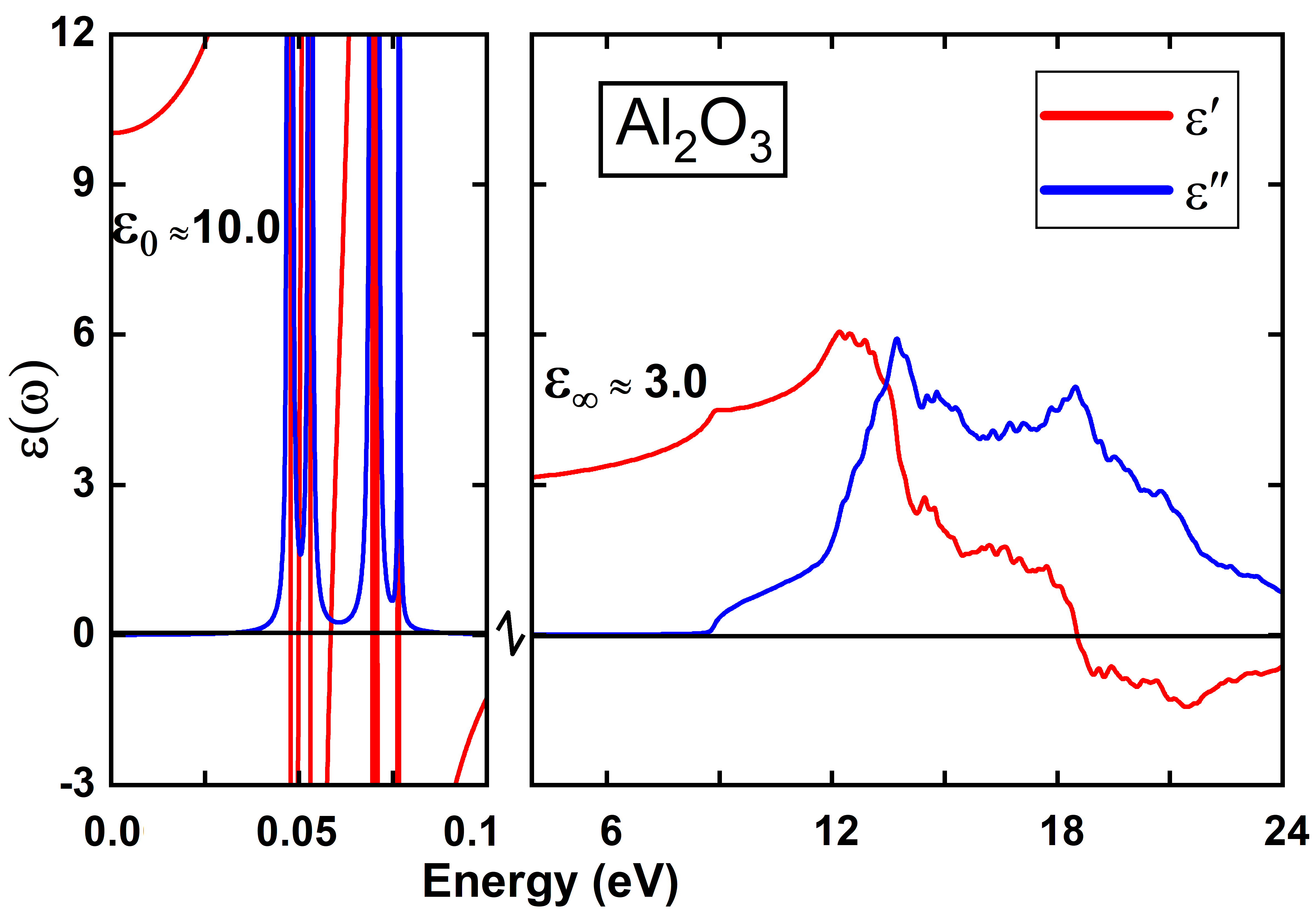
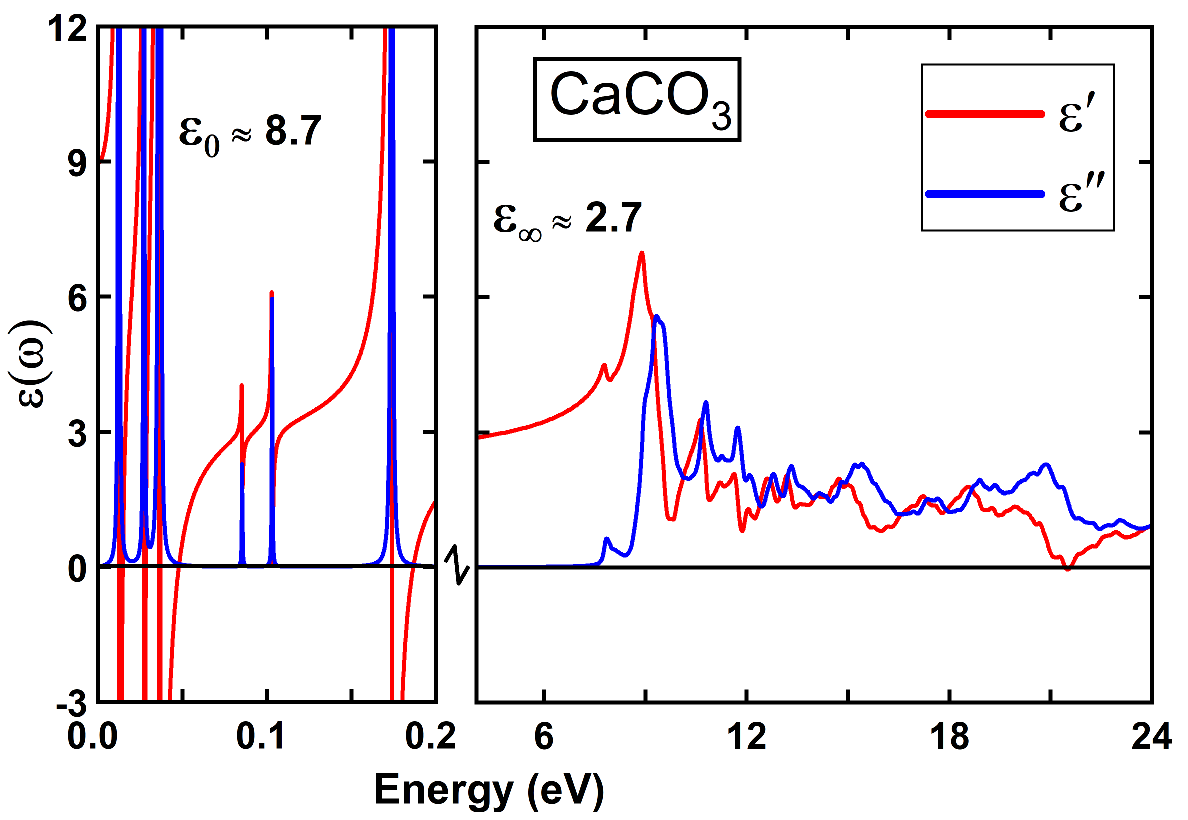
Figure 1: (Color online) Dielectric function of Al₂O₃ and CaCO₃. Left panel describes the vibrational contribution and the right panel describes the electronic transitions.

The dielectric response functions for alumina and calcite are presented in Fig. 1. The response due to electronic transitions contributes above the direct-gap energy on the eV scale, while the lattice dynamics contributes on the 0.1-eV scale; here, below 0.2 eV. We find that the PAW potential for Al with the electronic valence configuration $2s^{2}p^{6}3s^{2}p^{1}$ easily yields incorrect vibrational frequencies, and we, therefore, instead use the corresponding potential with the valence configuration $3s^{2}p^{1}$. As expected, CaCO₃ has a strong electronic response right above 9 eV, while Al₂O₃ has a smoother increase of the response up to the energy 14 eV. Since CaCO₃ constitutes both a lighter and a heavier cation, it is natural that the compound has vibrations that are both lower and higher in frequency than those of Al₂O₃. From the figure, one can observe that the two compounds have rather different dielectric functions, both in the regime of the vibrational contribution and for higher frequencies where the electronic transitions contribute. In SM,at [url will be inserted by publisher] for tables of the irreducible representations and detailed figures of the dielectric response functions. , we present the dielectric functions in more detail for both CaCO₃ and Al₂O₃, showing that there is only a moderate difference between the components in the perpendicular and the parallel directions. That is also obvious for the dielectric constants (Table 2). Both compounds have high-frequency constants from the electronic contribution that is close to 3. The optical vibration modes contribute to the static dielectric constant; this is somewhat larger for Al₂O₃ ($\sim 7.0$) compared to CaCO₃ ($\sim 6.0$). One can notice that the main difference is that Al₂O₃ has a much larger response in the parallel direction. Overall, there is a good agreement with the experimental findings, Young and Frederikse (1973) and the average static dielectric constant is calculated to be 10.0 in Al₂O₃, and 8.7 in CaCO₃.

Table 2: The static $\varepsilon_{0}$ and high-frequency $\varepsilon_{\infty}$ dielectric constants in the perpendicular, $\perp$, and parallel, $||$, ($z$-) direction. The average ($avg.$) data represents the arithmetic mean.

		DFT		Expt. Young and Frederikse (1973)
	$\perp$	$||$	$avg.$	$\perp$	$||$
Al2O3
$\varepsilon_{0}$	9.3	11.4	10.0	9.34	11.54
$\varepsilon_{\infty}$	3.0	3.0	3.0
CaCO3
$\varepsilon_{0}$	9.2	7.8	8.7	8.68, 8.5	8.31, 8.0
$\varepsilon_{\infty}$	2.9	2.3	2.7

IV.2 Sensitivity of DFT-based Hamaker constants for selected calcite systems

Before we set out to exploit the calculated dielectric functions at imaginary frequencies, we first explore how sensitive the results are to the low and high-frequency extrapolations methods.

The dielectric response for the Matsubara frequencies $\varepsilon(i\xi_{m})$ is obtained from the Kramers–Kronig relation as in Eq. 16. The calculated electronic structure from DFT implies energies up to about 250 eV, much higher than energies reached by standard experimental measurements with ellipsometers (typically, well below 10 eV). Higher energies have only small probability for excitation. However, in order to include high-energy transitions, we extrapolate the high-frequency tail of $\varepsilon(i\xi_{m})$ with a $1/\xi_{m}^{2}$ behaviour up to about 10 keV. With that extrapolation we can analyze the accuracy of the calculations of the Hamaker constants with respect to the number of Matsubara frequencies. Moreover, while the default calculations include semicore states down to 100 eV below the valence band maximum, we have also generated spectra of the dielectric functions with no semicore states for the cations Al and Ca, i.e., $3s^{2}p^{1}$ and $3p^{6}4s^{2}$ valence configurations, respectively. Those spectra are denoted by "no SC".

To analyze the importance to consider the optical phonons for small Matsubara frequencies (typically, $m<4$), we have generated diectric functions for which the vibrational contribution is completely neglected (those spectra are denoted by "no vib") but where the static dielectric constant is included for the $m=0$ term (denoted by "no vib with $\varepsilon_{0}$").

Parsegian and Ninham’s study Parsegian and Ninham (1969) in 1969 provided clear evidence that having partial knowledge of the optical spectra could sometimes be enough to make reasonable estimates of Hamaker constants and calculate the corresponding force. Assuming accurate model calculations using DFT, the extrapolation schemes mentioned earlier in this discussion yield very similar Hamaker constants for the calcite-ice-vapor system, with an accuracy of approximately 10%. According to the findings presented in Table 3, the predicted values for the calcite (1)-ice (2)-vapor (3) configuration are approximately A${}_{123}\sim-3.39\times 10^{-20}$ J and A${}_{123;0}\sim 0.26\times 10^{-20}$ J, where A_123;0 is the contribution from the zeroth Matsubara term of A₁₂₃.

Significant variations in precision are observed when calculating the Hamaker interaction for calcite-vapor-calcite at different temperatures, as indicated in Table 4. At lower temperatures, a greater number of Matsubara terms is required to cover the necessary upper-frequency range for achieving comparable accuracy. Utilizing only 500 Matsubara terms could result in a substantial 25% error in the calculated Hamaker constant. In Table 4, the "default", "noSC", and "no vib with $\varepsilon_{0}$" approximations all yield identical zero frequency Hamaker constants (as shown in the first row of Table 4). However, when vibrations are disregarded, the zero frequency Hamaker constant experiences a decrease of 0.045, 0.185, and 0.749$\times 10^{-20}$ J at temperatures of 70 K, 370 K, and 1500 K, respectively. It is crucial to highlight, however, that when considering different material combinations, such as cases where the dielectric functions of the materials intersect at certain frequencies or for the large separation behavior of gapped metals, Boström et al. the results become more reliant on the chosen approximations.

model	$m_{max}$	$A_{123}$ ($\rm 10^{-20}J$)	$A_{123;0}$ ($\rm 10^{-20}J$)
default	250	-3.088	0.260
	500	-3.332	0.260
	1000	-3.385	0.260
	1500	-3.391	0.260
	2000	-3.392	0.260
no SC	2000	-3.459	0.260
no vib	2000	-3.325	0.306
no vib with $\varepsilon_{0}$	2000	-3.371	0.260

Table 3: The Hamaker constants at 273.16 K using Eq.18, $A_{123}$ and its contributions from the zeroth Matsubara term $A_{123;0}$ for various three-layer configurations with CaCO₃ (1)-ice (2)-vapor (3) for different models CaCO₃ and using different cut-off Matsubara number ($m_{max}$).

model	$m_{max}$	70 K	370 K	1500 K
		$A_{123}$ ($\rm 10^{-20}J$)	$A_{123}$ ($\rm 10^{-20}J$)	$A_{123}$ ($\rm 10^{-20}J$)
default	0	0.0505	0.267	1.082
	500	10.441	14.316	14.970
	1000	13.051	14.430	14.972
	1500	13.802	14.442	14.972
	2000	14.078	14.445	14.972

Table 4: The Hamaker constants at different temperatures using Eq. 18, $A_{123}$ ($\rm 10^{-20}J$), in three-layer configurations with CaCO₃ (1)-vacuum (2)-CaCO₃ (3) using different cut-off Matsubara number ($m_{max}$) for the default dielectric function. The case with $m_{max}$=0 corresponds to the zero frequency Hamaker constant.

IV.3 Parameterised $\varepsilon(i\xi)$ for optimised data sets for calcite and alumina

To enable simple use of the calculated dielectric functions to study, for example, Casimir-Lifshitz interactions, we present parametrized average dielectric functions (see Table 5 for parameters) using a 14-mode oscillator model,Malyi et al. (2016) exploiting Eq. 20 but without any rotational relaxation. To be explicit we use the following model.

$$\varepsilon(i\xi)=1+\sum_{j}\frac{C_{j}}{1+(\xi/\omega_{j})^{2}}.$$ (24)

Here $\omega_{j}$ are the characteristic frequencies (given in $eV$ in the Table 5) and $C_{j}$ are proportional to the oscillator strengths. For ice and cold water ($T=273.16$ K) we use parameterised dielectric functions given in the literature.Fiedler et al. (2020); Luengo-Márquez and MacDowell (2021); Luengo-Marquez et al. (2022)

Table 5: Parametrization of the average dielectric function of continuous media, $\varepsilon(i\xi)$, at imaginary frequencies for Al₂O₃ and CaCO₃ as calculated with first-principles calculations. In this table frequencies are given in eV. The largest difference between fitted and calculated $\varepsilon(i\xi)$ is about 0.08$\%$.

$C_{j}$ and $\omega_{j}$ (in eV) for different compounds
Al2O3		CaCO3
modes ($\omega_{j}$)	coefficient ($C_{j}$)	modes ($\omega_{j}$)	coefficient ($C_{j}$)
0.0478	3.4263	0.0038	0.0879
0.0684	3.5999	0.0127	2.9661
1.1552	0.0015	0.035	2.6176
13.0704	1.0213	0.1696	0.4434
20.5561	0.8539	1.6088	0.0023
48.8508	0.0929	10.3375	0.8039
119.7988	0.0295	18.9299	0.6241
1288.9534	0.0	34.3621	0.2317
67441.835	0.0005	71.2998	0.0
102566.9502	0.0	81.1893	0.0221
407868.9726	0.0	84.7809	0.0
889915.6853	0.0	114.126	0.0
1723890.6517	0.0	124.3659	0.0
3447781.2791	0.0	241.5762	0.0005

IV.4 Casimir-Lifshitz force near alumina and calcite surfaces

The relationship between the retarded (distance-dependent) Hamaker constant and the retarded free energy, denoted as $A^{ret}(d)$ and $F(d,T)$ respectively, can be expressed as $A^{ret}(d)=-12\pi d^{2}\times F(d,T)$. This connection is illustrated in Figure 2 for various material combinations, including alumina-vacuum-alumina, calcite-vacuum-calcite, alumina-water-vapor, and calcite-water-vapor. The first two cases unequivocally confirm the well-known phenomenon where the interaction between identical surfaces is attractive and influenced by the material properties of the surfaces. Moreover, in situations involving the interface between a solid and a region with water vapor, there is a possibility of a short-range repulsion transitioning into a long-range attraction, that enables the formation of thin water films. In the latter two cases, where water serves as an intermediate layer, theoretical analysis suggests that in the presence of moisture (water vapour), a thin layer of water can indeed form on the outer surface of calcite, such as on soil particles. The corresponding free energy for these cases are presented in Figure 3. Interestingly, the systems exhibit energy minima for finite-sized water layers, further supporting the notion of water formation at these interfaces. At short separations, specifically when the finite velocity of light can be considered infinite, the product of reflection coefficients is proportional to

$$\frac{(\varepsilon_{1}-\varepsilon_{2})(\varepsilon_{3}-\varepsilon_{2})}{(\varepsilon_{1}+\varepsilon_{2})(\varepsilon_{3}+\varepsilon_{2})}.$$ (25)

This observation suggests that in cases where the dominating frequency range exhibits dielectric functions which fulfill $\varepsilon_{1}>\varepsilon_{2}>\varepsilon_{3}$, a repulsive interaction can occur. On the other hand, when the intermediate layer possesses a higher (or lower) dielectric function than both surrounding media within the dominant frequency range, an attractive force emerges. Analyzing the dielectric functions of water (which has an exceptionally high zero frequency dielectric constant) and calcite (whose dielectric function surpasses that of water at intermediate and high frequencies), we find that, through energy minimization, a Casimir-Lifshitz force can induce the formation of moisture on the surfaces of calcite (and alumina). This phenomenon, driven by Casimir-Lifshitz interactions, leads to the wetting of soil particles by water. In the subsequent subsection, we will further discuss how this Casimir-Lifshitz-induced water wetting affects the effective dielectric function of calcite soil particles.

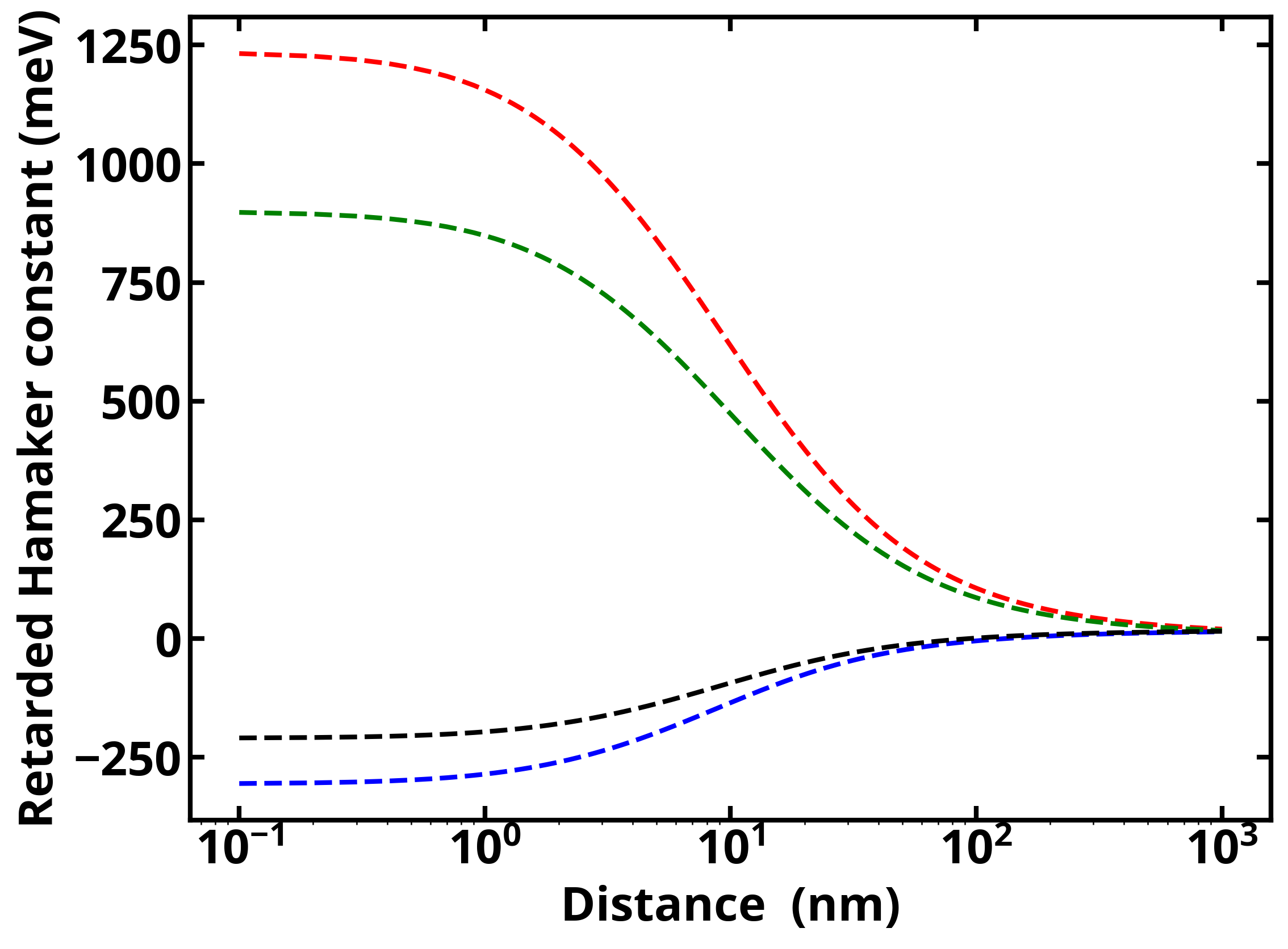
Figure 2: (Color online) The retarded Hamaker constant, $A^{ret}(d)=-F(d,T)\times 12\pi d^{2}$, for alumina-vacuum-alumina (red curve), calcite-vacuum-calcite (green curve), alumina-water-vapor (blue curve), and calcite-water-vapor (black curve). Temperature is 273.16 K, and other details are given in the text. The corresponding free energies in the region where blue and black curves cross over to positive values are studied in Fig. 3.

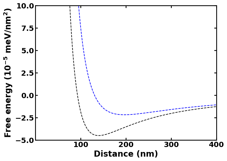
Figure 3: (Color online) The retarded free energy per unit area for two cases studied in Fig. 2 where energy minima are predicted: alumina-water-vapor (blue curve), and calcite-water-vapor (black curve). Temperature is 273.16 K, and other details are given in the text.

IV.5 Application to water and ice formation on calcite surfaces

In a pioneering paper, Elbaum and Schick Elbaum and Schick (1991) predicted that a minimum in the dispersion free energy of a thin liquid water film growing on ice would provide an explanation for observed partial melting on ice surfaces near the triple point of water. Following improvements of the modeling of water and ice dielectric functions,Fiedler et al. (2020); Luengo-Márquez and MacDowell (2021); Luengo-Marquez et al. (2022) further works explored this idea. These studies include ice melting and ice formation on ice nucleating particles in the atmosphere,Luengo-Márquez and MacDowell (2021); Luengo-Marquez et al. (2022) the modeling for anomalous stability of gas hydrates in ice cold water,Boström et al. (2021); Li et al. (2023) and ice formation/melting Fiedler et al. (2020); Esteso et al. (2020) on cold water surfaces. Some additional effects of temperature and intermolecular forces on ice adhesion have been discussed by Emelyanenko et al..Emelyanenko et al. (2022) An interesting idea to explore is the understanding of how the accumulation of ice-cold water or ice from available water vapor outside a calcite surface occurs at the triple point of water. This phenomenon is predicted to lead to the formation of either a thin water or ice film, resulting in a reduction of the overall free energy. Additionally, we identify a previously overlooked correction to the effective dielectric function of soil particles associated with this process. Addressing this aspect is crucial for the advancement of soil science models. To investigate this phenomenon, we utilize the dielectric functions for ice and cold water proposed by Luengo-Márquez and MacDowell.Luengo-Márquez and MacDowell (2021) The prediction based on Casimir-Lifshitz theory is that the growth of almost micron-sized ice or water layers is favored. For each calcite model considered in Table 3, the combination of calcite-ice-vapor results in an equilibrium ice layer with thickness d${}_{2}^{eq}$. Utilizing the retarded finite temperature Casimir-Lifshitz theory, the values for d${}_{2}^{eq}$ are found to be 0.151 $\mu$m, 0.153 $\mu$m, 0.121 $\mu$m, and 0.141 $\mu$m for the "default" calculations, "default noSC", "no vib", and "no vib with $\varepsilon_{0}$", respectively. These estimated thicknesses of approximately 0.12 $\mu$m to 0.15 $\mu$m are not significantly influenced by the number of terms included in the Matsubara summation, as long as a minimum of 500 terms is considered. Using the best available models for the dielectric functions of calcite and cold water,Luengo-Márquez and MacDowell (2021) we find that above the freezing point of water, the Lifshitz interaction promotes the existence of water vapor accumulating on the calcite surface leading to an $\sim 0.14\,\mu$m water film on the surface of soil particles. As an example, a calcite particle with a radius of $\sim 1\,\mu$m (neglecting curvature effects for demonstration purposes) could experience a volume increase of around 48% due to the presence of the wetting film. This phenomenon has implications for the effective dielectric function of soil, even in the absence of liquid water but in contact with water vapor. Notably, based on volume-averaged theory, the effective dielectric constant of a water-coated calcite particle would be approximately 34.8 for the specific example provided. Similarly, an ice coating with a thickness of approximately 0.15 $\mu$m would result in an effective dielectric constant of approximately 37.1. Figure 4 illustrates the estimated effective dielectric constants for calcite spheres coated with either ice or water as a function of the calcite particle’s radius. Above the freezing point of water, water can adsorb onto soil particles, while at the triple point of water, the growth of ice, water, or a combination thereof depends on the initial conditions. It is noteworthy that even for a calcite particle with a radius of 100 $\mu$m, the effective dielectric constant is enhanced by approximately 4% compared to the dielectric constant of pure calcite.

Figure 4: (Color online) The estimated effective dielectric constants for ice-coated calcite sphere (red dashed curve) and for water-coated calcite sphere (blue solid curve), both curves as functions of the bare calcite radius. Details are given in the text.

V Conclusions

Lebedew, in 1894, likely pioneered the connection between intermolecular forces and radiation processes.Lebedew (1894); Derjaguin et al. (2015) The theory linking optics and forces was subsequently established by Lifshitz and colleagues in their seminal papers.Lifshitz (1956); Dzyaloshinskii et al. (1961) Initially, incorporating optical data across a broad frequency range seemed challenging for achieving highly accurate force calculations. However, Parsegian and Ninham demonstrated that a few oscillator models for the dielectric function could yield reasonably good agreement between theory and experimental forces.Parsegian and Ninham (1969); Ninham et al. (1970); Richmond and Ninham (1971); Parsegian (2006); Ninham and Lo Nostro (2010) In our current study, we employed DFT to investigate the optical properties of two significant components, CaCO₃ and Al₂O₃, commonly found in diverse soil compositions. Our main objective was to investigate the influence of accurately describing the optical properties of these components on the formation of thin layers of water and ice on soil particles. This investigation carries significant scientific and engineering implications related to soil dynamics and related phenomena. Intriguingly, our findings reveal that the extrapolations made for low and high frequencies have minimal impact on the Hamaker constants and Lifshitz interactions. Importantly, all the extrapolations we investigated were reasonably accurate, as an inadequate extrapolation would lead to erroneous predictions for Casimir-Lifshitz forces and Hamaker constants, as evidenced by the divergent outcomes for the two materials. However, it is essential to acknowledge that the accuracy of these conclusions may vary for other systems, especially those characterized by crossings of different $\varepsilon(i\xi)$ functions at specific frequencies Elbaum and Schick (1991); Dou et al. (2014) or involving metallic components.Boström and Sernelius (2000); Boström et al. This work, along with prior research, establishes a direct link between optics derived from DFT and dispersion forces and their associated energies. We analyze these interactions and their impact on the formation of water and ice layers on soil particles in contact with moisture. Our findings reveal the previously unrecognized significance of this phenomenon in assessing soil water content, as highlighted by Lebron et al.. Lebron et al. (2004) Furthermore, our predictions hold substantial implications for future models concerning frost heave,Rempel (2007) as well as related effects such as cement storage and degradation in moist environments.  Weber and Reinhardt (1997)