Flexible Functional Treatment Effect Estimation

Abstract

We study treatment effect estimation with functional treatments where the average potential outcome functional is a function of functions, in contrast to continuous treatment effect estimation where the target is a function of real numbers. By considering a flexible scalar-on-function marginal structural model, a weight-modified kernel ridge regression (WMKRR) is adopted for estimation. The weights are constructed by directly minimizing the uniform balancing error resulting from a decomposition of the WMKRR estimator, instead of being estimated under a particular treatment selection model. Despite the complex structure of the uniform balancing error derived under WMKRR, finite-dimensional convex algorithms can be applied to efficiently solve for the proposed weights thanks to a representer theorem. The optimal convergence rate is shown to be attainable by the proposed WMKRR estimator without any smoothness assumption on the true weight function. Corresponding empirical performance is demonstrated by a simulation study and a real data application.

Keywords: Covariate balancing; functional data analysis; functional regression; reproducing kernel Hilbert space

1 Introduction

It is well known that for observational studies where a treatment is not randomly assigned, the estimation of average potential outcomes or contrasts (such as average treatment effects) is challenging due to possible confoundedness. This work focuses on estimating the treatment effect with a functional treatment, in contrast to the vast majority of existing work that focuses on binary and continuous treatments. For motivational purposes, we present a few examples as follows. To investigate the causal effect of temperature patterns in a year on crop yields in the following harvest season, one could use daily maximum and daily minimum temperature trajectories as functional treatments (Wong et al., 2019). To assess human visceral adipose tissue, Zhang et al. (2021) used body shape as a functional treatment and studied its causal effect on the tissue. In addition, biomedical researchers may be interested in the causal effect of the activity profile on certain health indicators, such as body mass index and waist circumference, which are potential indicators of obesity level (Neovius et al., 2005). The activity pattern of an individual can be recorded by a tracker during a certain time period, e.g., as in the Physical Activity Monitor data from the National Health and Nutrition Examination Survey (NHANES) in 2005-2006. One could transform a trajectory of activity intensity into a distribution of the intensity values (respresented by kernel mean embedding (Muandet et al., 2017)) and take it as a functional treatment. See Example 2 and Section 5.2 for more details.

There exists extensive literature on the estimation of average treatment effect (ATE) for binary treatments, which is well summarized by several review papers (e.g., Imbens, 2004; Stuart, 2010; Ding and Li, 2018; Yao et al., 2021). Extensions to multi-level categorical treatments (e.g., Yang et al., 2016; Lopez and Gutman, 2017; Li, 2019) and continuous treatments (e.g., Robins et al., 2000; Hirano and Imbens, 2004; Imai and van Dyk, 2004; Imai and Ratkovic, 2014; Galvao and Wang, 2015; Zhu et al., 2015; Kennedy et al., 2017; Fong et al., 2018; Li et al., 2020; Bahadori et al., 2022) are also abundant. Although there is practical interest in the causal effect of functional variables, existing methods that can be applied directly to functional treatments are scarce. To the best of our knowledge, only three related works (Zhao et al., 2018; Zhang et al., 2021; Tan et al., 2022) are devoted to estimating the causal effects of functional treatments using observational data, but each has limitations that we seek to address. We will contrast our proposed method with these works in detail below. We note that functional variables are sometimes treated as confounders (e.g., McKeague and Qian, 2014; Laber and Staicu, 2018; Ciarleglio et al., 2018; Miao et al., 2022) and outcomes (Zhao et al., 2018; Lin et al., 2021). Such settings are fundamentally different from ours, where the functional variables are treatments, accompanied with vector-valued covariates and a real-valued outcome.

With an unconfoundedness assumption, two modeling strategies are commonly adopted to estimate causal effects. One is the outcome regression approach, which first estimates an outcome regression model by treating both the treatments and confounders as predictors, and then averages the regression prediction on a fixed treatment value over the observed covariate distribution. The functional linear model, the most common scalar-on-function model, is often employed for this purpose (Zhao et al., 2018). However, due to the limited flexibility in characterizing the outcome given the functional treatment and multivariate covariates using the functional linear model, inconsistent estimation can arise from model misspecifications. Although some complex scalar-on-function regression models are available, model misspecification still pose a major risk for causal effect estimation. The other approach is based on estimating weights that directly address the selection bias of functional treatments. Compared to the regression approach, weighting methods try to mimic randomized experiments that theoretically balance on all pre-treatment-assignment variables, and do not involve the direct use of outcome data in constructing weights. As a result, they help to preserve the objectivity of the analysis and avoid data snooping (Rubin, 2007; Rosenbaum et al., 2010). We adopt the weighting approach in this paper.

One of the biggest challenges in weighting for causal effect estimation of functional treatments is that, unlike discrete or continuous variables, the density of functional treatment is not well established due to its intrinsically infinite dimension (Delaigle and Hall, 2010). This phenomenon also prevents a direct adaptation of existing estimators for continuous treatment effects which often requires estimating density functions. To overcome this issue, we define a weight function through reverse conditioning that is well-defined for functional treatments and properly adjusts for the selection bias. We also propose a novel estimation approach that directly computes weights via the idea of covariate balancing. Covariate balancing has recently become a popular approach in causal inference for observational studies due to its advantage of providing a stable estimation of weights. For example, covariate balancing methods have been developed for binary treatments (e.g., Hainmueller, 2012; Imai and Ratkovic, 2014; Qin and Zhang, 2007; Zubizarreta, 2015; Wong and Chan, 2018; Wang and Zubizarreta, 2020) and continuous treatments (e.g., Fong et al., 2018; Kallus and Santacatterina, 2019; Tübbicke, 2022), and for estimating conditional treatment effects (e.g., Wang et al., 2022).

Zhang et al. (2021) and Tan et al. (2022) also adopt the idea of covariate balancing to estimate the causal effect of functional treatments by weighting, but with several weaknesses. The approach by Zhang et al. (2021) relies on a finite approximation of the functional treatment by truncating the tail part of its functional principal components. The weights are estimated by balancing the correlation between the covariates and the top functional principal components, which is directly generalized from Fong et al. (2018) to handle continuous treatments. This approach has several drawbacks. First, there is likely information loss in selecting only several top functional principal components. Second, only balancing the correlation may not be enough to guarantee the consistency of the final causal effect estimator unless the true outcome regression has a certain simple parametric form in the selected top functional principal components. Furthermore, the theoretical properties of their approach are not studied. Instead of using an approximation of the functional treatment, Tan et al. (2022) construct functional stabilized weights by balancing a set of growing number of basis functions. However, they focus on a functional linear marginal structural model, which imposes additional structure to the causal effect which may well be misspecified. Compared with Zhang et al. (2021) and Tan et al. (2022), our proposed covariate balancing method is distinct in the following aspects. (1) Our proposed method does not rely on any finite approximation of the functional treatment. (2) The balancing weights are constructed to directly balance the difference between the final causal effect estimator and the true target function. (3) We do not require a linear functional marginal structural model. (4) Our estimator attains the optimal rate of convergence under mild conditions. We will further elaborate on these points as follows.

Inspired by the development in nonparametric functional regression under the framework of reproducing kernel Hilbert space (RKHS) (e.g., Kadri et al., 2010; Zhang et al., 2012; Oliva et al., 2015; Szabó et al., 2016; Kadri et al., 2016), we adopt the RKHS modeling for the functional treatment effects, which allows for a great flexibility (compared to a functional linear marginal structural model) in characterizing the effect of different functional treatments. In particular, we assume that the marginal structural model lies in an RKHS of functions with a functional input. With the help of the closed-form solution of weight-modified kernel ridge regression (WMKRR), we then propose balancing weights that are capable of controlling the balancing error between a smoothed weighted average and the population mean of functionals in a large hypothesis class (see (9) for the explicit form). We will then show that the solution to the optimization objective lies in a finite-dimensional space by a representer theorem and that the resulting optimization is convex. The theoretical analysis of the balancing error is not a trivial generalization from that for the binary treatment effects, since the balancing structure is significantly more complicated due to the interplay between weighting and smoothing in the formulation, and the balancing error is a function with a functional input instead of a scalar. Furthermore, while ignored by Zhang et al. (2021) and Tan et al. (2022), a functional treatment is often not fully observable in practice and thus requires some pre-processing steps for recovery, which creates another layer of complication in the theoretical analysis. We provide a careful and detailed theoretical analysis to deal with all these complications. Asymptotic properties of the proposed estimator are derived under the complex dependency structure of the weights and kernel ridge regression. Under appropriate technical conditions, we are able to show that the proposed causal effect estimator can achieve the optimal nonparametric convergence rate, without additional modeling assumptions on the true weight function.

The rest of the paper is organized as follows. Section 2.1 provides the basic setup of the weight-modified kernel ridge regression. Section 2.2 introduces the construction of covariate balancing weights for functional treatments. Computational details and an algorithm to construct the proposed balancing weights are presented in Section 3. Section 4 develops the asymptotic properties of the proposed weighted estimator. The numerical performance of the proposed method is demonstrated by a simulation study in Section 5.1 and an application to a physical activity tracking data set in Section 5.2.

2 Functional Treatment Effect Estimation

2.1 Background and motivation

Let $A\in\mathcal{A}$ be a functional treatment defined on $\mathcal{T}$, and $\bm{X}\in\mathcal{X}\subseteq\mathbb{R}^{p}$ be a $p$-dimensional confounder. Denote by $Y(a)\in\mathbb{R}$ the potential outcome had treatment $a$ was given, for $a\in\mathcal{A}$. Suppose that $\{(A_{i},\bm{X}_{i},Y_{i}(\cdot)):i=1,\dots,n\}$ are independent and identically distributed copies of $(A,\bm{X},Y(\cdot))$. In practice, we do not observe all the potential outcomes per subject. In fact, only one particular case is observed. The observed outcome for the $i$-th subject is $Y_{i}:=Y_{i}(A_{i})$. As such, the available data is $\{(A_{i},\bm{X}_{i},Y_{i}):i=1,\dots,n\}$. The goal is to estimate the functional treatment effect (FTE):

$$\tau(a):=\mathbb{E}\{Y(a)\},\qquad a\in\mathcal{A}.$$

Note that the domain of $\tau$ is a possibly infinite-dimensional function space $\mathcal{A}$, and therefore (non-parametric) estimations of $\tau$ are significantly harder than typical continuous treatment estimations. Throughout the paper, we impose the following two assumptions.

Assumption 1 (Weak unconfoundedness).

Let $D(a)$ be the indicator of receiving treatment $a$: $D(a)=1$ if $A=a$; $D(a)=0$ otherwise. We have

$$Y(a)\ \mbox{$\perp\!\!\!\perp$}\ D(a)\mid\bm{X},\mathrm{\ for\ any\ }a\in\mathcal{A}.$$

This assumption is the weak unconfoundedness assumption introduced in Imbens (2000), which only requires the pairwise independence of the treatment with each of the potential outcomes. It is less restrictive than the strong ignorability assumption (Rosenbaum and Rubin, 1983): $\{Y(a),a\in\mathcal{A}\}\ \mbox{$\perp\!\!\!\perp$}\ A\mid\bm{X}$.

Take $\rho_{U}$ as the marginal distribution of a random object $U$, and $\rho_{U\mid V}$ as the conditional distribution of $U$ given $V$. Define the weight function $w^{*}$ as

$$w^{*}(a,\bm{x}):=\frac{\rho_{\bm{X}}(\bm{x})}{\rho_{\bm{X}\mid A}(\bm{x}\mid a)},$$ (1)

which can be used to adjust the dependence between the treatment $A$ and the confounder $\bm{X}$. In (1), we use densities of the covariates $\bm{X}$ instead of the densities of the treatment $A$, as is commonly done in ATE methods (e.g., Wong and Chan, 2018; Kennedy et al., 2017). As such, we are able to circumvent the challenge of establishing functional densities (Delaigle and Hall, 2010). Based on the definition of $w^{*}$, one can observe that

$$\mathbb{E}\{w^{*}(A,\bm{X})Y\mid A=a\}=\mathbb{E}\left[w^{*}(a,\bm{X})\mathbb{E}(Y\mid A=a,\bm{X})\mid A=a\right]$$

$$= \mathbb{E}\left[w^{*}(a,\bm{X})\mathbb{E}(Y(a)\mid A=a,\bm{X})\mid A=a\right]=\mathbb{E}\left[w^{*}(a,\bm{X})\mathbb{E}(Y(a)\mid D(a)=1,\bm{X})\mid A=a\right]$$

$$= \mathbb{E}\left[w^{*}(a,\bm{X})\mathbb{E}(Y(a)\mid\bm{X})\mid A=a\right]=\mathbb{E}\left\{\frac{\rho_{\bm{X}}(\bm{X})}{\rho_{\bm{X}\mid A}(\bm{X}\mid a)}\mathbb{E}(Y(a)\mid\bm{X})\mid A=a\right\}$$

$$= \int_{\bm{x}}\frac{\rho_{\bm{X}}(\bm{x})}{\rho_{\bm{X}\mid A}(\bm{x}\mid a)}\mathbb{E}(Y(a)\mid\bm{X}=\bm{x})\rho_{\bm{X}\mid A}(\bm{x}\mid a)\mathrm{d}{\bm{x}}=\int_{\bm{x}}\rho_{\bm{X}}(\bm{x})\mathbb{E}(Y(a)\mid\bm{X}=\bm{x})\mathrm{d}{\bm{x}}=\mathbb{E}\{Y(a)\}.$$

Intuitively, this means that the weight function $w^{*}$ helps to adjust the conditional expectation of the observed outcome $Y$ so that the weight-modified outcome $Z:=w^{*}(A,\bm{X})Y$ is an unbiased observation of the treatment effect. This indicates that one can regress $Z$ on $A$ to recover $\tau$. In addition to Assumption 1, we also require the following overlap condition:

Assumption 2 (Overlap).

There exists a positive constant $C_{1}\ltx@label{cnt:overlapupper}$ such that $w^{*}(a,\bm{x})\leq C_{\ref*{cnt:overlapupper}}$ for all $a\in\mathcal{A},\bm{x}\in\mathcal{X}$.

This assumption plays a similar role as the standard positivity assumption of the conditional treatment density under the settings of continuous treatments (e.g., Assumption 2 in Kennedy et al., 2017). If the true weights $w^{*}_{i}:=w^{*}(A_{i},\bm{X}_{i})$, $i=1,\dots,n$, are known and the functional treatments $A_{i}$, $i=1,\dots,n$, are fully observed, we can construct the adjusted outcomes $Z_{i}=w^{*}_{i}Y_{i}$ such that $\mathbb{E}(Z_{i}\mid A_{i})=\tau(A_{i})$ for every $i$, and then perform a regression over the data $\{(A_{i},Z_{i}),i=1,\dots,n\}$ to estimate $\tau$. Here we consider a nonparametric regression model that allows for a flexible modeling for $\tau$. In particular, we assume that $\tau$ lies in an RKHS ${\mathcal{H}}_{A}$ with a reproducing kernel $K_{A}(\cdot,\cdot)$, with the corresponding inner product $\langle\cdot,\cdot\rangle_{{\mathcal{H}}_{A}}$ and norm $\|\cdot\|_{{\mathcal{H}}_{A}}$ respectively.

Remark 1.

Note that the reproducing kernel $K_{A}$ is a bivariate function with function inputs. Based on an additional assumption that $\mathcal{A}$ is a Hilbert space, we provide some concrete examples of $K_{A}$ that are easy to implement in practice. Recall that its inner product and norm are denoted by $\langle\cdot,\cdot\rangle_{\mathcal{A}}$ and $\|\cdot\|_{\mathcal{A}}$ respectively. The linear kernel $K_{A}(A_{1},A_{2})=\langle A_{1},A_{2}\rangle_{\mathcal{A}}+c$ with a constant $c$ is probably the simplest example. Its corresponding RKHS $\mathcal{H}_{A}$ contains linear functions of the form $\beta_{0}+\langle\beta_{1},\cdot\rangle_{\mathcal{A}}$, where $\beta_{0}\in\mathbb{R}$ and $\beta_{1}\in\mathcal{A}$. As for nonlinear kernels, examples include the Gaussian kernel with $K_{A}(A_{1},A_{2})=\exp\{-2\|A_{1}-A_{2}\|_{\mathcal{A}}^{2}/\theta\}$ and exponential kernel with $K_{A}(A_{1},A_{2})=\exp\{-\|A_{1}-A_{2}\|_{\mathcal{A}}/\theta\}$ respectively for some pre-specified $\theta>0$.

We consider the weight-modified kernel ridge regression (WMKRR) estimator for $\tau$:

$$\tilde{\tau}:=\operatorname*{argmin}_{\tau\in{\mathcal{H}}_{A}}\frac{1}{n}\sum_{i=1}^{n}\left(w^{*}_{i}Y_{i}-\tau(A_{i})\right)^{2}+\lambda\|\tau\|^{2}_{{\mathcal{H}}_{A}},$$ (2)

where $\lambda>0$ is a tuning parameter of the regularization. In (2), the norm $\|\cdot\|_{{\mathcal{H}}_{A}}$ in the penalty term measures the “roughness” of the underlying mapping, and therefore encourages a “smoother” solution to (2) as $\lambda$ increases.

Unfortunately, the true weights $w^{*}_{i}$, $i=1,\dots,n$, are typically unknown in observational studies. A natural solution is to first directly estimate $w^{*}_{i}$ based on its definition, and then construct the adjusted outcomes based on these estimates. This has been extensively studied in ATE estimation when the treatment $A$ is a binary random variable (e.g., Feng et al., 2012; Hirano et al., 2003). However, this approach has several drawbacks. First, from the definition of $w^{*}$ in (1), the estimation of $w^{*}$ involves estimating the densities of $\bm{X}$ and $\bm{X}\mid A$. Even if one uses a finite approximation of $A$ (see Remark 2 below), their estimations are still challenging. This is because to make Assumption 1 plausible, $\bm{X}$ should include all the confounders that affect both the treatment and outcome, so it is usually multivariate. This indicates that estimating multivariate density functions is required, which is known to be difficult: Parametric estimations of multivariate density functions have a risk of possible model misspecifications, while nonparametric estimations such as the kernel density estimation suffer from slow rates of convergence in multivariate settings. Second, the true weights are expected to achieve the balance for covariates in expectation. However, it is unclear if such balance is enough for finite samples, especially when the sample size is small and the covariates are sparse (Zubizarreta et al., 2011). Third, the inverse of the densities can result in instability, especially when the estimated densities are close to zero.

To overcome the aforementioned problems, we consider finding a stable set of weights that mimic the role of $w^{*}_{i}$, $i=1,\dots,n$, through the idea of covariate balancing. There exists extensive literature on covariate balancing techniques for ATE estimation when the treatment is binary (e.g. Hainmueller, 2012; Imai and Ratkovic, 2014; Qin and Zhang, 2007; Zubizarreta, 2015; Wong and Chan, 2018; Wang and Zubizarreta, 2020) or continuous (e.g. Fong et al., 2018; Kallus and Santacatterina, 2019; Tübbicke, 2022), while we consider covariate balancing for the challenging setup where the treatment is functional.

Remark 2.

Zhang et al. (2021) introduce functional propensity scores that are based on the functional principal components (FPCs) of $A$ and define balancing weights based on the lower-order FPCs. Then the input of the weight function becomes finite-dimensional, which resembles the setting of multivariate continuous treatments. However, this definition relies on the unsupervised dimension reduction of the process $A$ and has the risk of missing important information. For example, if the higher-order FPC scores are more correlated with the potential outcome than the lower-order ones, their proposed weight that only depends on the latter may not properly account for all confounding. In contrast, our method to be shown below does not rely on such unsupervised truncation of $A$ so it can avoid the information loss mentioned above.

Remark 3.

Tan et al. (2022) introduce a functional stabilized weight (FSW) estimator. They consider a functional linear marginal structural model $\tau(a)=\alpha+\int_{\mathcal{T}}\beta(t)a(t)\mathrm{d}t$ for some scalar $\alpha$ and function $\beta$, which is restrictive and subject to the risk of model misspecifications. Instead of directly estimating the weight function $w^{*}$, they estimate its projection $w^{*}(a,\cdot):\mathcal{X}\rightarrow\mathbb{R}$ for every fixed $a\in\mathcal{A}$ by attempting to maintain the covariate balance $\mathbb{E}\{w^{*}(a,\bm{X})b(\bm{X})\}=\mathbb{E}\{b(\bm{X})\}$ for any integrable function $b$. A Nadaraya-Watson estimator is proposed to approximate the left-hand side of the equation. To obtain the sequence of estimated weights, they have to perform the optimization $n$ times, separately for each observation. The convergence of their estimated weights depends on the smoothness of the projection $w^{*}(a,\cdot)$. In contrast, as shown below, our method does not require the restrictive linearity assumption above for the marginal structural model. Moreover, our proposed weights are calculated jointly via a single optimization, and we do not require any smoothness assumption for the function $w^{*}$. Furthermore, the final weighted causal effect estimator can achieve the optimal rate of convergence with a nonparametric modeling of $\tau$, i.e., without assuming a linear functional marginal structural model on $\tau$.

2.2 Construction of weights

To motivate our construction, first suppose we have obtained a set of adjusted weights $\bm{w}=[w_{1},\dots,w_{n}]^{\intercal}$. From (2), we form an estimator of the treatment effect:

$$\hat{\tau}_{\bm{w}}:=\operatorname*{argmin}_{\tau\in{\mathcal{H}}_{A}}\frac{1}{n}\sum_{i=1}^{n}\left(w_{i}Y_{i}-\tau(A_{i})\right)^{2}+\lambda\|\tau\|^{2}_{{\mathcal{H}}_{A}}.$$ (3)

Recall that ${\mathcal{H}}_{A}$ is the RKHS with the reproducing kernel $K_{A}$. We give the following definition which will be useful in expressing and analyzing the solution of (3).

Definition 1.

For $a\in\mathcal{A}$, $\mathcal{K}_{a}:\mathbb{R}\rightarrow{\mathcal{H}}_{A}$ is a Hilbert-Schmidt operator such that

$$f(a)=\mathcal{K}_{a}^{*}f=\langle K_{A}(a,\cdot),f\rangle_{{\mathcal{H}}_{A}},$$

where $\mathcal{K}_{a}^{*}$ is the adjoint of $\mathcal{K}_{a}$. Define the operator $\mathcal{S}_{a}:=\mathcal{K}_{a}\mathcal{K}_{a}^{*}$. Note that we have

$$\mathcal{S}_{a}:{\mathcal{H}}_{A}\rightarrow{\mathcal{H}}_{A},\qquad(\mathcal{S}_{a}f)(\cdot)=f(a)K_{A}(a,\cdot)\mathrm{\ for\ any\ }f\in{\mathcal{H}}_{A}.$$

With Definition 1, the estimator (3) can be rewritten as:

$$\hat{\tau}_{\bm{w}}=\left(\frac{1}{n}\sum_{i=1}^{n}\mathcal{S}_{A_{i}}+\lambda\mathcal{I}\right)^{-1}\left(\frac{1}{n}\sum_{i=1}^{n}\mathcal{K}_{A_{i}}w_{i}Y_{i}\right),$$ (4)

where $\mathcal{I}:{\mathcal{H}}_{A}\rightarrow{\mathcal{H}}_{A}$ is an identity operator such that $\mathcal{I}f=f$ for any $f\in{\mathcal{H}}_{A}$. See, e.g., Caponnetto and De Vito (2007) and Smale and Zhou (2007) for more details.

Define $m(a,\bm{x})=\mathbb{E}\{Y(a)\mid A=a,\bm{X}=\bm{x}\}=\mathbb{E}\{Y(a)\mid\bm{X}=\bm{x}\}$. We can then express

$$Y_{i}(a)=m(a,\bm{X}_{i})+\epsilon_{i}(a),\qquad i=1,\dots,n,$$ (5)

where $\epsilon_{i}(a)=Y_{i}(a)-m(a,\bm{X}_{i})$ satisfies $\mathbb{E}[\epsilon_{i}(a)\mid A_{i}=a,\bm{X}_{i}]=\mathbb{E}[\epsilon_{i}(a)\mid\bm{X}_{i}]=0$. This allows the error to be heteroskedastic with respect to the functional treatment and other covariates, and leads to $\tau(a)=\mathbb{E}_{X\sim\rho_{X}}\{m(a,X)\}$. We assume that $\mathbb{E}[\epsilon^{2}_{i}(a)\mid\bm{X}_{i}]\leq\sigma_{0}^{2}<\infty$ for some constant $\sigma_{0}>0$ (not depending on $\bm{X}_{i}$, $a$ and $i$). As $(Y_{i}(a),\bm{X}_{i})$, $i=1,\dots,n$, are i.i.d., so are $\epsilon_{i}(a)$, $i=1,\dots,n$. According to (5), the observed data follow

$$Y_{i}=Y_{i}(A_{i})=m(A_{i},\bm{X}_{i})+\epsilon_{i}(A_{i})=m(A_{i},\bm{X}_{i})+\epsilon_{i},\qquad i=1,\dots,n,$$ (6)

where we write $\epsilon_{i}=\epsilon(A_{i})$ for short. Clearly, $\mathbb{E}(\epsilon_{i}\mid A_{i}=a,\bm{X}_{i})=\mathbb{E}(\epsilon_{i}(a)\mid A_{i}=a,\bm{X}_{i})=\mathbb{E}(\epsilon_{i}(a)\mid\bm{X}_{i})=0$ and, similarly, $\mathbb{E}(\epsilon_{i}^{2}\mid A_{i}=a,\bm{X}_{i})\leq\sigma_{0}^{2}$. As such, $\mathbb{E}(\epsilon_{i}\mid A_{i},\bm{X}_{i})=0$, $\mathbb{E}(\epsilon_{i}^{2}\mid A_{i},\bm{X}_{i})\leq\sigma_{0}^{2}$. Following (6), we can decompose the difference between $\hat{\tau}_{\bm{w}}$ and $\tau$ as:

$$\hat{\tau}_{\bm{w}}-\tau= \left(\frac{1}{n}\sum_{i=1}^{n}\mathcal{S}_{A_{i}}+\lambda\mathcal{I}\right)^{-1}\left(\frac{1}{n}\sum_{i=1}^{n}\mathcal{K}_{A_{i}}w_{i}Y_{i}\right)-\tau=I_{1}+I_{2},$$

$$\text{where}\quad I_{1} =\left(\frac{1}{n}\sum_{i=1}^{n}\mathcal{S}_{A_{i}}+\lambda\mathcal{I}\right)^{-1}\left(\frac{1}{n}\sum_{i=1}^{n}\mathcal{K}_{A_{i}}w_{i}m(A_{i},\bm{X}_{i})\right)-\tau,$$ (7)

$$\text{and}\quad I_{2} =\left(\frac{1}{n}\sum_{i=1}^{n}\mathcal{S}_{A_{i}}+\lambda\mathcal{I}\right)^{-1}\left(\frac{1}{n}\sum_{i=1}^{n}\mathcal{K}_{A_{i}}w_{i}\epsilon_{i}\right).$$ (8)

Apparently the estimation error of $\hat{\tau}_{\bm{w}}$ can be bounded by properly controlling the magnitudes of $I_{1}$ in (7) and $I_{2}$ in (8). Roughly speaking, term (8) exhibits concentration (at zero) due to the independence among $\epsilon_{i}$’s conditional on the treatments and covariates. This will be rigorously shown in our theoretical analysis. The primary challenge lies in controlling (7) since $m$ is unknown in practice. To address this, motivated by Wong and Chan (2018), Kallus and Santacatterina (2019) and Wang et al. (2022), we assume that $m$ belongs to a certain class of functions and control (7) for every element in this class.

Explicitly, we assume that $m$ lies in a tensor-product RKHS ${\mathcal{H}}:={\mathcal{H}}_{A}\otimes{\mathcal{H}}_{X}$ of functions defined on $\mathcal{A}\times\mathcal{X}$. Here ${\mathcal{H}}_{X}$ is an RKHS of functions defined on $\mathcal{X}$, with a reproducing kernel $K_{X}$ and its corresponding inner product and norm of ${\mathcal{H}}_{X}$ are denoted by $\langle\cdot,\cdot\rangle_{{\mathcal{H}}_{X}}$ and $\|\cdot\|_{{\mathcal{H}}_{X}}$ respectively. Note that the assumption $m\in{\mathcal{H}}={\mathcal{H}}_{A}\otimes{\mathcal{H}}_{X}$ is compatible with the aforementioned assumption $\tau\in{\mathcal{H}}_{A}$ due to the following proposition.

Proposition 1.

Under Assumption 5 in Section 4, if $\sup_{u\in{\mathcal{H}}_{X}}|\mathbb{E}u(\bm{X})|\neq 0$, we have ${\mathcal{H}}_{A}=\{\mathbb{E}_{\bm{X}\sim\rho_{X}}g(\cdot,\bm{X}):g\in{\mathcal{H}}\}$.

To bound the magnitude of (7), we aim to find weights $\tilde{\bm{w}}=[\tilde{w}_{1},\dots,\tilde{w}_{n}]^{\intercal}$ such that

$$\Upsilon:=\sup_{u\in{\mathcal{H}}:\|u\|_{\mathcal{H}}\leq 1}\left\|\left(\frac{1}{n}\sum_{i=1}^{n}\mathcal{S}_{A_{i}}+\lambda\mathcal{I}\right)^{-1}\left(\frac{1}{n}\sum_{i=1}^{n}\mathcal{K}_{A_{i}}\tilde{w}_{i}u(A_{i},\bm{X}_{i})\right)-\mathbb{E}_{\bm{X}\sim\rho_{\bm{X}}}u(\cdot,\bm{X})\right\|$$ (9)

is minimized with respect to some norm $\|\cdot\|$. Note that the objective (i.e., the norm) of the supremum (9) is proportional to $\|u\|_{\mathcal{H}}$. Therefore, we limit the space to ${\mathcal{H}}(1)=\{u\in{\mathcal{H}}:\|u\|_{{\mathcal{H}}}\leq 1\}$. Since $\tau(a)=\mathbb{E}_{\bm{X}\sim\rho_{\bm{X}}}m(a,\bm{X})$ and $m\in\mathcal{H}$, we have

$$\left\|\left(\frac{1}{n}\sum_{i=1}^{n}\mathcal{S}_{A_{i}}+\lambda\mathcal{I}\right)^{-1}\left(\frac{1}{n}\sum_{i=1}^{n}\mathcal{K}_{A_{i}}\tilde{w}_{i}m(A_{i},\bm{X}_{i})\right)-\tau\right\|\leq\Upsilon\|m\|_{{\mathcal{H}}}.$$

Since $\|m\|_{\mathcal{H}}<\infty$, bounding (9) provides a good control over the discrepancy (7) even if we do not know the true outcome function $m$.

While $\bm{\tilde{w}}$ is well motivated, the criterion in (9) is not directly applicable for the following reasons. First, $\mathbb{E}_{\bm{X}\sim\rho_{\bm{X}}}u(\cdot,\bm{X})$ is usually unavailable since the distribution of $\bm{X}$ is unknown. Thus we propose to replace it with its empirical counterpart $\sum_{i=1}^{n}u(\cdot,\bm{X}_{i})/n$. Second, the norm $\|\cdot\|$ in (9) needs to be chosen. A natural choice is $\mathcal{L}_{2}(A)$-norm $\|\cdot\|_{\mathcal{L}_{2}}$ defined by $\|f\|_{\mathcal{L}_{2}}=\sqrt{\mathbb{E}\{f^{2}(A)\}}$ for a function $f:\mathcal{A}\to\mathbb{R}$. In practice, we will use the empirical norm $\|\cdot\|_{n}$, which is defined by $\|f\|_{n}:=\sqrt{\sum_{k=1}^{n}f^{2}(A_{k})/n}$. Finally, the functional treatments are often not fully observed in practice so we will need to recover $A_{i}$ by $\hat{A}_{i}$. Two examples of $\hat{A}_{i}$ will be given in Examples 1 and 2 below.

By the above discussion, we use the following criterion for controlling (7):

$$Q(\bm{w},\lambda,u):=\left\|\left(\frac{1}{n}\sum_{i=1}^{n}\mathcal{S}_{\hat{A}_{i}}+\lambda\mathcal{I}\right)^{-1}\left(\frac{1}{n}\sum_{i=1}^{n}\mathcal{K}_{\hat{A}_{i}}w_{i}u(\hat{A}_{i},\bm{X}_{i})\right)-\frac{1}{n}\sum_{j=1}^{n}u(\cdot,\bm{X}_{j})\right\|_{n}^{2}.$$ (10)

In addition, to simultaneously control the second moment of (8), we introduce the following regularization term of the weights:

$$R(\bm{w},\lambda)=\frac{1}{n^{2}}\sum_{i=1}^{n}w_{i}^{2}\left\|\left(\frac{1}{n}\sum_{j=1}^{n}\mathcal{S}_{\hat{A}_{j}}+\lambda\mathcal{I}\right)^{-1}\mathcal{K}_{\hat{A}_{i}}\right\|_{n}^{2}.$$ (11)

Combining (10) and (11), we define the proposed balancing weights as

$$\bm{\hat{w}}=[\hat{w}_{1},\dots,\hat{w}_{n}]^{\intercal}:=\operatorname*{argmin}_{0\leq w_{i}\leq L,i=1,\dots,n}\left[\sup_{u\in{\mathcal{H}}(1)}\{Q(\bm{w},\lambda,u)\}+\eta R(\bm{w},\lambda)\right],$$ (12)

where ${\mathcal{H}}(1)=\{u\in{\mathcal{H}}:\|u\|_{{\mathcal{H}}}\leq 1\}$, $\eta\geq 0$ is a tuning parameter and $L$ is an upper bound for the estimated weights and is allowed to be infinity. In sequel, we write $\hat{\tau}$ in short for $\hat{\tau}_{\hat{\bm{w}}}$ when $\hat{\bm{w}}$ is computed from (12).

Before we conclude this section, we provide some examples of $\hat{A}_{i}$ to recover $A_{i}$ in practice, $i=1,\dots,n$.

Example 1.

Densely observed trajectories. For every $A_{i}\in\mathcal{A}$, $i=1,\ldots,n$, its noisy observations $\{\gamma_{i,j}:j=1,\dots,N\}$ are measured at $\{t_{i,j}:j=1,\dots,N\}$, a dense grid of $\mathcal{T}$. More specifically, $\gamma_{i,j}=A_{i}(t_{i,j})+\varepsilon_{i,j}$, where $\mathbb{E}(\varepsilon_{i,j})=0$. Under certain assumptions on the grid points, e.g., $t_{i,j}$, $j=1,\dots,N$, are i.i.d. copies of a random variable $T$ with density $\rho_{T}$, common nonparametric regression procedures can be applied to each individual $i$ to obtain $\hat{A}_{i}$, such as penalized spline regression (e.g. Griggs, 2013) and smoothing spline regression (e.g. Rice and Rosenblatt, 1983).

Example 2.

Kernel mean embedding of distributions. If we want to use a distribution as a treatment (e.g., the activity profile as mentioned in Section 1), we can let $A$ be the kernel mean embedding of the distribution (e.g., Muandet et al., 2017). More specifically, for the $i$-th individual, the kernel mean embedding $A_{i}$, $i=1,\ldots,n$, is defined by

$$A_{i}=\int_{\mathcal{T}}K_{e}(\cdot,t)\mathrm{d}P_{i}(t),$$

where $P_{i}$ is the corresponding distribution function, and $K_{e}:\mathcal{T}\times\mathcal{T}\rightarrow\mathbb{R}$ is a reproducing kernel. Suppose that we have i.i.d. samples $t_{i,l}$, $l=,\dots,N$, drawn from $P_{i}$. Then we can take $\hat{A}_{i}$ as the empirical embedding

$$\hat{A}_{i}=\frac{1}{N}\sum_{l=1}^{N}K_{e}(\cdot,t_{i,l}).$$

3 Computational Details

In this section, we discuss the computation for (12).

3.1 Representer theorem, closed-form expression and convexity

3.1.1 Inner optimization

First, let us focus on the inner optimization of (12), i.e., $\sup_{u\in{\mathcal{H}}(1)}Q(\bm{w},\lambda,u)$. Note that it is an infinite-dimensional optimization problem when ${\mathcal{H}}$ is infinite dimensional. The practical optimization relies on the following representer theorem, which shows that the solution indeed lies in a finite-dimensional space given data.

Theorem 1 (Representer theorem).

The solution to $\sup_{u\in{\mathcal{H}}(1)}Q(\bm{w},\lambda,u)$ lies in the finite-dimensional space

$${\mathcal{H}}_{n}:=\left\{\sum_{i=1}^{n}\alpha_{i}K_{A}(\cdot,\hat{A}_{i})K_{X}(\cdot,\bm{X}_{i})+\sum_{i=1}^{n}\beta_{i}K_{A}(\cdot,\hat{A}_{i})\left(\frac{1}{n}\sum_{j=1}^{n}K_{X}(\cdot,\bm{X}_{j})\right):\alpha_{i},\beta_{i}\in\mathbb{R}\right\}.$$

With Theorem 1, we are able to take a further step and obtain a closed-form representation of $\sup_{u\in{\mathcal{H}}(1)}Q(\bm{w},\lambda,u)$. Define

$$\begin{split}\bm{G}_{A}:=[K_{A}(\hat{A}_{i},\hat{A}_{j})]_{i,j=1}^{n}\in\mathbb{R}^{n\times n};\qquad\bm{G}_{X}:=[K_{X}(\bm{X}_{i},\bm{X}_{j})]_{i,j=1}^{n}\in\mathbb{R}^{n\times n};\\ \bar{\bm{G}}_{X}:=\left[\frac{1}{n}\sum_{j=1}^{n}K_{X}(\bm{X}_{i},\bm{X}_{j})\right]_{i=1}^{n}\in\mathbb{R}^{n};\qquad\bar{g}_{X}:=\frac{1}{n^{2}}\sum_{i=1}^{n}\sum_{j=1}^{n}K_{X}(\bm{X}_{i},\bm{X}_{j}).\end{split}$$ (13)

Then, for any $u\in{\mathcal{H}}_{n}$, $Q(\bm{w},\lambda,u)$ can be written as

$$Q(\bm{w},\lambda,u)= \frac{1}{n}\big{\|}\bm{G}_{A}\left(\bm{G}_{A}+n\lambda\bm{I}\right)^{-1}\left[\bm{w}\circ\left\{\left(\bm{G}_{A}\circ\bm{G}_{X}\right)\bm{\alpha}+\left(\bm{G}_{A}\odot\bar{\bm{G}}_{X}^{\intercal}\right)^{\intercal}\bm{\beta}\right\}\right]$$

$$-\left[\left(\bm{G}_{A}\odot\bar{\bm{G}}_{X}^{\intercal}\right)\bm{\alpha}+\bar{g}_{X}\bm{G}_{A}\bm{\beta}\right]\big{\|}_{2}^{2},\quad\text{for some $\bm{\alpha}\in\mathbb{R}^{n}$ and $\bm{\beta}\in\mathbb{R}^{n}$,}$$

where $\circ$ is the element-wise product between matrices (vectors), $\odot$ is the column-wise Khatri-Rao product, and $\|\cdot\|_{2}$ is the Euclidean norm of a vector.

We next simplify the constraint $u\in{\mathcal{H}}(1)$ in maximizing $Q(\bm{w},\lambda,u)$. By Theorem 1, it suffices to only focus on the squared RKHS norm of a function $u\in{\mathcal{H}}_{n}$, which can be expressed as

$$\left\|\sum_{i=1}^{n}\alpha_{i}K_{A}(\cdot,A_{i})K_{X}(\cdot,\bm{X}_{i})+\sum_{i=1}^{n}\beta_{i}K_{A}(\cdot,A_{i})\left(\frac{1}{n}\sum_{j=1}^{n}K_{X}(\cdot,\bm{X}_{j})\right)\right\|^{2}_{\mathcal{H}}=\bm{\gamma}^{\intercal}\bm{G}_{F}\bm{\gamma},$$

where $\bm{\gamma}=[\bm{\alpha}^{\intercal},\bm{\beta}^{\intercal}]^{\intercal}\in\mathbb{R}^{2n}$ and

$$\bm{G}_{F}=\begin{bmatrix}\bm{G}_{A}\circ\bm{G}_{X}&\left(\bm{G}_{A}\odot\bar{\bm{G}}_{X}^{\intercal}\right)^{\intercal}\\ \bm{G}_{A}\odot\bar{\bm{G}}_{X}^{\intercal}&\bar{g}_{X}\bm{G}_{A}\\ \end{bmatrix}\in\mathbb{R}^{2n\times 2n}.$$

Note that we can decompose $\bm{G}_{F}$ as

$$\bm{G}_{F}=\bm{M}\bm{M}^{\intercal}=\begin{bmatrix}\bm{M}_{1}\\ \bm{M}_{2}\\ \end{bmatrix}[\bm{M}_{1}^{\intercal},\bm{M}_{2}^{\intercal}],$$

where $\bm{M}\in\mathbb{R}^{2n\times q}$, $\bm{M}_{1},\bm{M}_{2}\in\mathbb{R}^{n\times q}$, $q\leq 2n$. Thus finally, we have

$$\sup_{u\in{\mathcal{H}}(1)}Q(\bm{w},\lambda,u)= \frac{1}{n}\sup_{\bm{\gamma}^{\intercal}\bm{G}_{F}\bm{\gamma}=1}\left\|\bm{G}_{A}\left(\bm{G}_{A}+n\lambda\right)^{-1}\bm{I}\left\{\mathrm{diag}(\bm{w})\bm{M}_{1}\bm{M}^{\intercal}\bm{\gamma}\right\}-\left(\bm{M}_{2}\bm{M}^{\intercal}\right)\bm{\gamma}\right\|_{2}^{2}$$

$$= \frac{1}{n}\sup_{\|\bm{M}\bm{\gamma}\|_{2}=1}(\bm{M}^{\intercal}\bm{\gamma})^{\intercal}\left\{\bm{G}_{A}\left(\bm{G}_{A}+n\lambda\bm{I}\right)^{-1}\mathrm{diag}(\bm{w})\bm{M}_{1}-\bm{M}_{2}\right\}^{\intercal}$$

$$\qquad\left\{\bm{G}_{A}\left(\bm{G}_{A}+n\lambda\right)^{-1}\mathrm{diag}(\bm{w})\bm{M}_{1}-\bm{M}_{2}\right\}(\bm{M}^{\intercal}\bm{\gamma})$$

$$= \frac{1}{n}\left[\sigma_{\max}\left\{\bm{G}_{A}\left(\bm{G}_{A}+n\lambda\bm{I}\right)^{-1}\mathrm{diag}(\bm{w})\bm{M}_{1}-\bm{M}_{2}\right\}\right]^{2},$$ (14)

where $\sigma_{\max}(\cdot)$ returns the largest singular value of the input matrix. As such, (14) is the closed-form representation of the objective function in the inner optimization of (12).

3.1.2 Convexity with respect to weights

We next show that the objective function in (12) is convex with respect to $\bm{w}$. First, the regularization term $R(\bm{w},\lambda)$ in the outer minimization is a quadratic function of $\bm{w}$ and hence convex in $\bm{w}$. Moreover, the inner maximization has been rewritten as in (14), and its convexity in $\bm{w}$ is implied by the following lemma.

Lemma 1.

For fixed $\bm{A}\in\mathbb{R}^{n\times n}$, $\bm{B}\in\mathbb{R}^{n\times q}$ and $\bm{D}\in\mathbb{R}^{n\times q}$, the function $\varrho(\bm{w})=\left[\sigma_{\max}\left\{\bm{A}\mathrm{diag}(\bm{w})\bm{B}-\bm{D}\right\}\right]^{2}$ is a convex function.

Finally, we collect the previous results and express (12) in a practical optimization form. Notice that

$$R(\bm{w},\lambda)=\frac{1}{n^{2}}\sum_{i=1}^{n}w_{i}^{2}\left\|\left(\frac{1}{n}\sum_{i=1}^{n}\mathcal{S}_{A_{i}}+\lambda\mathcal{I}\right)^{-1}\mathcal{K}_{A_{i}}\right\|_{n}^{2}=\sum_{j=1}^{n}w_{j}^{2}\left\{\frac{1}{n}\sum_{i=1}^{n}\left\{\left[\bm{G}_{A}\left(\bm{G}_{A}+n\lambda\bm{I}\right)^{-1}\right]_{i,j}\right\}^{2}\right\},$$ (15)

where $\bm{A}_{i,j}$ indicates the $(i,j)$-th element of matrix $\bm{A}$. Therefore we can show that (12) is equivalent to

$$\begin{split}\hat{\bm{w}}=\operatorname*{argmin}_{0<w_{i}<L,i=1,\dots,n}\frac{1}{n}\left[\sigma_{\max}\left\{\bm{G}_{A}\left(\bm{G}_{A}+n\lambda\bm{I}\right)^{-1}\mathrm{diag}(\bm{w})\bm{M}_{1}-\bm{M}_{2}\right\}\right]^{2}\\ +\eta\sum_{j=1}^{n}w_{j}^{2}\left\{\frac{1}{n}\sum_{i=1}^{n}\left\{\left[\bm{G}_{A}\left(\bm{G}_{A}+n\lambda\bm{I}\right)^{-1}\right]_{i,j}\right\}^{2}\right\}.\end{split}$$ (16)

Due to the convexity of the objective function, common algorithms such L-BFGS-B can be applied to solve (16) given the smoothing parameter $\lambda$ and tuning parameter $\eta$.

3.2 Tuning parameter selection

Here we discuss how to select $\lambda$ and $\eta$. The smoothing parameter $\lambda$ needs to be provided in order to calculate the balancing error (10), and hence the weights. Recall that the weights are used to form a modified outcome for the WMKRR. Naturally, one would tune $\lambda$ based on common methods for kernel ridge regression such as cross-validation, but this becomes very difficult in our case because of the complicated dependency between the weights and $\lambda$. To address this issue, we propose a simple solution which performs reasonably well in practice. The idea is to use a simple estimator of the adjusted response to guide the selection of $\lambda$. More specifically, we first obtain the adjusted responses with the FCBPS weights described in Zhang et al. (2021), as their weights do not depend on $\lambda$ and can be computed quickly. Then we apply the leave-one-out cross-validation (LOOCV) to select $\lambda$ based on the mean square error computed in the validation set. Finally we use the selected $\lambda$ to compute the proposed weights without updating $\lambda$ further.

As for the hyper-parameter $\eta$, it is related to the magnitude of weights so as to achieve a balance between (7) and (8). Here we propose to use a fitted outcome regression to help select the best $\eta$. To be specific, we fit a KRR to get an estimate for $m$, and denote it as $\hat{m}$. Then we take $\hat{\tau}_{\texttt{REG}}=\frac{1}{n}\sum_{i=1}^{n}\hat{m}(\cdot,\bm{X}_{i})$ as the estimator for $\tau$ from the regression approach. Denote by $\hat{w}_{i}^{(\eta)}$, $i=1,\dots,n$, the weights defined in (12) for each given $\eta$. We select the best $\eta$ such that

$$V(\eta):=\left\|\left(\frac{1}{n}\sum_{i=1}^{n}\mathcal{S}_{\hat{A}_{i}}+\lambda\mathcal{I}\right)^{-1}\left(\frac{1}{n}\sum_{i=1}^{n}\mathcal{K}_{\hat{A}_{i}}\hat{w}^{(\eta)}_{i}\hat{m}(\hat{A}_{i},\bm{X}_{i})\right)-\hat{\tau}_{\texttt{REG}}\right\|_{n}^{2}\\ +\left\|\left(\frac{1}{n}\sum_{i=1}^{n}\mathcal{S}_{\hat{A}_{i}}+\lambda\mathcal{I}\right)^{-1}\left[\frac{1}{n}\sum_{i=1}^{n}\mathcal{K}_{\hat{A}_{i}}\hat{w}^{(\eta)}_{i}\left\{Y_{i}-\hat{m}(\hat{A}_{i},\bm{X}_{i})\right\}\right]\right\|_{n}^{2}$$ (17)

is the smallest. In Algorithm 1 in Section A in the supplementary material, we summarize the computation steps to obtain the proposed $\hat{\eta}$ with tuning parameter selection.

4 Theory

In this section we provide the rate of convergence for $\hat{\tau}$. We first introduce a few notations and assumptions. Given two Hilbert spaces $\mathcal{V}$ and $\mathcal{W}$, the operator norm of an operator $B\in\mathcal{L}(\mathcal{V},\mathcal{W})$ is defined as $\|B\|_{\mathcal{L}(\mathcal{V},\mathcal{W})}:=\sup_{\|v\|_{\mathcal{V}}\leq 1}\|Bv\|_{\mathcal{W}}$.

Assumption 3.

$\{(A_{i},\bm{X}_{i},\epsilon_{i}(a),a\in\mathcal{A}),i=1,\dots,n\}$ are independent. For any $a\in\mathcal{A}$, $\mathbb{E}(\epsilon_{i}(a)|A_{i},\bm{X}_{i})=0$ for $i=1,\dots,n$, and $\sup_{1\leq i\leq n}\mathbb{E}(\epsilon_{i}(a)^{2}|A_{i},\bm{X}_{i})\leq\sigma^{2}_{0}$ for some constant $\sigma_{0}>0$.

Assumption 4.

$\tau\in{\mathcal{H}}_{A}$ and $m\in{\mathcal{H}}$.

Assumption 5.

$K_{X}$ and $K_{A}$ are positive definite kernels. $K_{X}$ is continuous and the real function $(a_{1},a_{2})\mapsto\langle\mathcal{K}_{a_{1}}c_{1},\mathcal{K}_{a_{2}}c_{2}\rangle_{{\mathcal{H}}_{A}}$ is measurable for any $c_{1},c_{2}\in\mathbb{R}$. There exists a constant $C_{2}\ltx@label{cnt:kernelbound}>0$ such that $\sup_{a\in\mathcal{A}}|K_{A}(a,a)|\leq C_{2}$ and $\sup_{\bm{x}\in\mathcal{X}}|K_{X}(\bm{x},\bm{x})|\}\leq C_{\ref*{cnt:kernelbound}}$.

Assumption 6.

Either one of the following two conditions is satisfied.

1. Functional treatments $A_{i}$, $i=1,\dots,n$, are fully observed without error. In this case, we take $\hat{A}_{i}=A_{i}$. This corresponds to $\kappa=0$ in (18) below.

2. There exists a pseudometric $d:\mathcal{A}\times\mathcal{A}\to[0,\infty)$ such that:

   1. The mapping $\mathcal{K}_{(\cdot)}:\mathcal{A}\rightarrow\mathcal{L}(\mathbb{R},{\mathcal{H}}_{A})$ is Hölder continuous, i.e., there exist constants $H>0$ and $0<h\leq 1$ such that

      $$\|\mathcal{K}_{a_{1}}-\mathcal{K}_{a_{2}}\|_{\mathcal{L}(\mathbb{R},{\mathcal{H}}_{A})}\leq H[d(a_{1},a_{2})]^{h},\quad a_{1},a_{2}\in\mathcal{A}.$$

   2. All $\hat{A}_{1},\dots,\hat{A}_{n}$ are independent. Each $\hat{A}_{i}$ can estimate $A_{i}$ at a uniform rate $\kappa=\kappa(n)$ over $i=1,\dots,n$, i.e.,

      $$\max_{1\leq i\leq n}d(\hat{A}_{i},A_{i})=\mathop{}\mathopen{}\mathcal{O}\mathopen{}_{\mathrm{p}}\left(\kappa\right).$$ (18)

Assumption 3 is a standard assumption for the data, which allows for heteroscedasticity of the errors. Assumption 4 states that the function classes for the target function $\tau$ and the outcome model $m$ are well-specified. Assumption 5 is a boundedness requirement for the reproducing kernels. It is satisfied for the majority of common kernels including Gaussian and exponential kernels discussed in Remark 1. As for Assumption 6, we only need one of the two specified conditions. When all functional treatments are fully observed without error (Assumption 6(a)), there is no need to recover $A_{i}$. So we can simply take $\hat{A}_{i}=A_{i}$. Otherwise, we need to recover $A_{i}$ by $\hat{A}_{i}$. Assumption 6(b) specifies the related conditions for $\hat{A}_{i}$ in this case: the Hölder continuity of the operator $\mathcal{K}_{a}$ and rate of convergence for $\hat{A}_{i}$. For example, when we take $d$ in Assumption 6(b) as the norm $\|\cdot\|$ used in constructing the kernel in Remark 1, the Gaussian kernel and exponential kernel mentioned in Remark 1 satisfy the Hölder continuity condition with $h=1$ and $h=1/2$ respectively. See Table 1 in Szabó et al. (2016) for more examples. As for the rate of convergence $\kappa$, it can be specified given different applications. As in Example 1 in Section 2.2, if every $A_{i}$, $i=1,\ldots,n$, satisfies $\int_{\mathcal{T}}A_{i}^{2}(t)\rho_{T}(t)\mathrm{d}t<\infty$ ($\rho_{T}$ was defined as in Example 1), one can fix the norm $\|f\|=[\int_{\mathcal{T}}f^{2}(t)\rho_{T}(t)\mathrm{d}t]^{1/2}$ for each $f\in\mathcal{A}$ and obtain a nonparametric convergence rate for $\kappa$ with typical nonparametric regression approaches. For example, when $A_{i}$ is a twice-differentiable univariate function, under appropriate assumptions, the smoothing spline regression can lead to $\kappa=N^{-2/5}\log n$ (Raskutti et al., 2012), where $\log n$ is due to the union bound over $n$ functions. In Example 2 in Section 2.2, when $\hat{A}_{i}$, $i=1,\ldots,n$, are empirical kernel embeddings, one can take $\|\cdot\|=\|\cdot\|_{{\mathcal{H}}_{e}}$, the RKHS norm of the kernel embeddings associated with the reproducing kernel $K_{e}$, and let $\kappa=N^{-1/2}\log n$. See Section A.1.10 in Szabó et al. (2015) for more detailed results.

We introduce additional terms before presenting the last technical assumption. Define $\mathcal{S}_{a}=\mathcal{K}_{a}\mathcal{K}_{a}^{*}$ and let $\mathcal{S}=\mathbb{E}_{A\sim\rho_{A}}\mathcal{S}_{A}$. Define the trace norm $\mathrm{Tr}(\cdot)$ of a semi-positive-definite operator $B:\mathcal{B}\rightarrow\mathcal{B}$ as $\mathrm{Tr}(B)=\sum_{l}\langle Be^{\mathcal{B}}_{l},e^{\mathcal{B}}_{l}\rangle_{\mathcal{B}}$ with $\{e^{\mathcal{B}}_{l}\}$ an orthonormal basis of $\mathcal{B}$. Under Assumption 5, $\mathrm{Tr}(\mathcal{S})\leq\sup_{a\in\mathcal{A}}\mathrm{Tr}(\mathcal{S}_{a})\leq C_{\ref*{cnt:kernelbound}}$. Then the spectral theorem yields

$$\mathcal{S}=\sum_{l=1}^{L}t_{l}\langle\cdot,e_{l}\rangle_{{\mathcal{H}}_{A}}e_{l},$$ (19)

where $\{e_{l}\}_{l=1}^{L}\subset\mathcal{{\mathcal{H}}_{A}}$ such that $\langle e_{l},e_{l^{\prime}}\rangle_{{\mathcal{H}}_{A}}=1$ if $l=l^{\prime}$ and 0 otherwise, and $t_{1}\geq t_{2}\geq\dots\geq t_{L}>0$, with $\sum_{l=1}^{L}t_{l}=\mathrm{Tr}(\mathcal{S})\leq C_{\ref*{cnt:kernelbound}}$. Here $L$ can be $\infty$. We also define

$$\mathcal{N}(\lambda):=\mathrm{Tr}\{(\mathcal{S}+\lambda\mathcal{I})^{-1}\mathcal{S}\}=\sum_{l=1}^{\infty}\frac{t_{l}}{t_{l}+\lambda}.$$

As to be shown in the theorems below, the rate of convergence for $\hat{\tau}$ depends on the decay of the eigenvalues of $\mathcal{S}$. We also note that the theorems below hold for general choices of kernels.

Theorem 2.

Under Assumptions 1–6, if $\mathcal{N}(\lambda)(\lambda n)^{-1}=\mathop{}\mathopen{}\mathcal{O}\mathopen{}(1)$, $\lambda\leq\|\mathcal{S}\|_{\mathcal{L}({\mathcal{H}}_{A})}$, $\kappa^{2h}=\mathop{}\mathopen{}\mathcal{O}\mathopen{}(\lambda\mathcal{N}(\lambda)n^{-1})$, $\kappa^{h}=\mathop{}\mathopen{}\mathcal{O}\mathopen{}(\lambda)$ and $\sqrt{\sum_{l=1}^{\infty}\min\{t_{l},\lambda\}}(\sqrt{n}\lambda)^{-1}=\mathop{}\mathopen{}\mathcal{O}\mathopen{}(1)$, we have

$$\sup_{u\in{\mathcal{H}}(1)}Q(\hat{\bm{w}},\lambda,u)=\mathop{}\mathopen{}\mathcal{O}\mathopen{}_{\mathrm{p}}\left[(1+\eta)\frac{\mathcal{N}(\lambda)}{n}+\lambda\right],$$ (20)

$$\text{and}\quad R(\hat{\bm{w}},\lambda)=\mathop{}\mathopen{}\mathcal{O}\mathopen{}_{\mathrm{p}}\left[\frac{\mathcal{N}(\lambda)}{n}+\eta^{-1}\left(\frac{\mathcal{N}(\lambda)}{n}+\lambda\right)\right],$$ (21)

where $\hat{\bm{w}}:=(\hat{w}_{1},\dots,\hat{w}_{n})^{\intercal}$.

Theorem 2 provides the orders of the balancing error (10) and the regularization (11) with respect to $\hat{\bm{w}}$. Based on Theorem 2, we can develop the rate of convergence for the proposed weighted estimator $\hat{\tau}$. For instance, if the decay of eigenvalues of $\mathcal{S}$ follows a polynomial rate as shown in Assumption 7 below, we are able to achieve a nonparametric convergence rate for $\tau$.

Assumption 7.

There exists a constant $b>1$ such that $t_{l}\asymp l^{-b}$ for any $l\geq 1$.

This decay rate is also considered in Caponnetto and De Vito (2007) and Szabó et al. (2016).

Theorem 3.

Suppose that the conditions stated in Theorem 2 hold. Then

$$\|\hat{\tau}-\tau\|_{n}=\mathop{}\mathopen{}\mathcal{O}\mathopen{}_{\mathrm{p}}\left(\sigma_{0}\eta^{-1/2}\left(\frac{\mathcal{N}(\lambda)}{n}+\lambda\right)^{1/2}+\left(\frac{\mathcal{N}(\lambda)}{n}\right)^{1/2}\right)\|m\|_{\mathcal{H}}.$$

If we further assume Assumption 7 hold,

$\lambda\asymp n^{-b/(1+b)}$, $\|\mathcal{S}\|_{\mathcal{L}({\mathcal{H}}_{A})}\geq\lambda$, $\kappa=\mathop{}\mathopen{}\mathcal{O}\mathopen{}(n^{-b/[h(1+b)]})$ and $\eta\asymp 1$, then there exists some constant $C_{b}>0$ such that

$$\mathcal{N}(\lambda)\leq C_{b}\lambda^{-1/b}.$$

Also, we have

$$\left\|\hat{\tau}-\tau\right\|_{n}=\mathop{}\mathopen{}\mathcal{O}\mathopen{}_{\mathrm{p}}\left(n^{-\frac{b}{2(1+b)}}\right)\|m\|_{{\mathcal{H}}}.$$

Theorem 3 provides the rate of convergence for $\hat{\tau}$ under Assumption 7. According to Caponnetto and De Vito (2007), this rate is minimax in estimating the target function $\tau\in{\mathcal{H}}_{A}$ using the i.i.d data $\{A_{i},w^{*}_{i}Y_{i}\}_{i=1}^{n}$.

Remark 4.

The proposed causal effect estimator, based on $\bm{\hat{w}}$, enjoys the same minimax rate of convergence as the ordinary kernel ridge regression estimator using the modified outcome $\{w^{*}_{i}Y_{i}\}_{i=1}^{n}$ with the true but unknown weights. However, the theoretical analysis with weights obtained by (12) is significantly more complicated than the typical analysis for kernel ridge regression. One reason is that the responses in kernel ridge regression are typically assumed independent, while the adjusted responses $\hat{w}_{i}Y_{i}$ are all dependent since $\bm{\hat{w}}$ are obtained by (12). Moreover, as we do not impose any modeling assumption of $\bm{w^{*}}$, the convergence between $\bm{\hat{w}}$ and $\bm{w^{*}}$ cannot be established or used to show the convergence of WMKRR. Instead we perform a careful analysis to control the uniform error $\sup_{u\in{\mathcal{H}}(1)}Q(\bm{\hat{w}},\lambda,u)$, which leads to the convergence for $\hat{\tau}$.

5 Numerical Studies

5.1 Simulation

We first compare the finite-sample performance of different estimators via a simulation study. We have $200$ simulated datasets where $n=200$ independent subjects are generated in each simulated data. The observations $(A_{i},{\bm{X}_{i}},Y_{i})$ for the $i$-th subject, $i=1,\ldots,n$, in each simulated data are i.i.d. copies of $(A,{\bm{X}},Y)$ as below. We assume the functional variables $A_{i}$’s are fully observed. The confounders $\bm{X}=[X^{(1)},X^{(2)},X^{(3)},X^{(4)}]^{\intercal}\in\mathbb{R}^{4}$ follow the multivariate normal distribution with the zero mean vector and the identity covariance matrix. The functional treatment $A$ is generated by $A(t)=\sum_{k=1}^{4}A^{(k)}\sqrt{2}\sin(2\pi kt)$, $t\in[0,1]$, where $A^{(1)}\mid\bm{X}\sim N(4X^{(1)},1)$, $A^{(2)}\mid\bm{X}\sim N(2\sqrt{3}X^{(2)},1)$, $A^{(3)}\mid\bm{X}\sim N(2\sqrt{2}X^{(3)},1)$ and $A^{(4)}\mid\bm{X}\sim N(2X^{(4)},1)$.

The outcome $Y$ is generated by $Y\mid(A,\bm{X})\sim N(m(A,\bm{X}),1)$, where we consider three choices for $m$ as follows. Let $\Psi(\bm{x})=x^{(2)}(x^{(1)})^{2}+(x^{(4)})^{2}\sin(2x^{(3)})$ where $\bm{x}=[x^{(1)},x^{(2)},x^{(3)},x^{(4)}]^{\intercal}$ and $\mu(t)=2\sqrt{2}\sin(2\pi t)+\sqrt{2}\cos(2\pi t)+\sqrt{2}\sin(4\pi t)/2+\sqrt{2}\cos(4\pi t)/2$.

• Setting 1: We let $m(a,\bm{x})=15\Psi(\bm{x})+\int_{t=0}^{1}a(t)\mu(t)\mathrm{d}t.$ In this case, the treatment effect $\tau(a)$ is linear in $a$ in the sense

  $$\tau(a)=\int_{t=0}^{1}a(t)\mu(t)\mathrm{d}t,$$

  and $m$ is additive in $\Psi(\bm{x})$ and $a$.

• Setting 2: We let $m(a,\bm{x})=10\Psi(\bm{x})+0.5(a^{(1)})^{2}+4\sin(a^{(1)}).$ Here $m$ is additive in $\Psi(\bm{x})$ and $a$. Then the treatment effect is

  $$\tau(a)=0.5(a^{(1)})^{2}+4\sin(a^{(1)}),$$

  which is nonlinear in $a$.

• Setting 3: We let $m(a,\bm{x})=[1+2/3\Psi(\bm{x})][0.5(a^{(1)})^{2}+4\sin(a^{(1)})].$ In this case, the treatment effect $\tau(a)$ has the same form as in Setting 3, but $\Psi(\bm{x})$ interacts with $a$ in $m$.

In this simulation study, we compare the following estimators for $\tau$.

1. CFB: our proposed (KRR) estimator where weights are obtained from (12).

2. FCBPS: the weighted least squares estimator proposed in Zhang et al. (2021) where the weights are based on the parametric SFPS estimation described in Zhang et al. (2021). Here, the parametric modeling of the relevant densities is correctly specified.

3. NPFCBPS: the weighted least squares estimator proposed in Zhang et al. (2021) where the weights are obtained by using the non-parametric SFPS estimation described in Zhang et al. (2021).

4. REG: the regression estimator $\hat{\tau}_{\texttt{REG}{}}$ discussed in Section 3.2.

5. NW: the estimator without adjusting the response, i.e., $w_{i}^{*}Y_{i}$ in (2) is replaced by the original response $Y_{i}$ for $i=1,\dots,n$.

When performing the KRR for CFB, REG and NW, we take $K_{A}$ and $K_{X}$ both as Gaussian kernels. More specifically, $K_{A}(a_{1},a_{2})=(\sqrt{2\pi}\sigma_{A})^{-1}\exp\{-\int_{t=0}^{1}(a_{1}(t)-a_{2}(t))^{2}\mathrm{d}t/\sigma_{A}^{2}\}$ and $K_{X}(\bm{x}_{1},\bm{x}_{2})=(\sqrt{2\pi}\sigma_{X})^{-1}\exp\{-(\bm{x}_{1}-\bm{x}_{2})^{\intercal}(\bm{x}_{1}-\bm{x}_{2})/\sigma_{X}^{2}\}$, where $\sigma_{A}$ and $\sigma_{X}$ are selected by the median heuristic (Fukumizu et al., 2009; Garreau et al., 2017). For FCBPS and NPFCBPS, the number of FPC $L$ is chosen such that the top $L$ FPC scores explain $95\%$ percentage of the variance. Both FCBPS and NPFCBPS assume a linear model for $\tau$. Therefore only Setting 1 is correctly specified for them. For CFB, we select its tuning parameter by the procedure described in Section 3 (or Algorithm 1 in the supplementary material) For REG and NW, we use LOOCV to select the smoothing parameter $\lambda$ in KRR.

Two evaluation metrics are provided to assess the performance of these estimators. Take $\tau^{\prime}$ as a generic estimator of $\tau$.

1. Empirical MSE: the mean squared errors (MSE) on sample points: $\sum_{i=1}^{n}[\tau(A_{i})-{\tau^{\prime}}(A_{i})]^{2}/n$.

2. Out-of-Sample MSE: the mean squared errors (MSE) measured on a set of new evaluation points: $\sum_{i=1}^{n^{\prime}}[\tau(A^{\prime}_{i})-{\tau^{\prime}}(A^{\prime}_{i})]^{2}/{n^{\prime}}$, where $n^{\prime}=100$ and $A_{i}^{\prime}(t)=\sum_{k=1}^{4}A_{i}^{\prime(k)}\sqrt{2}\sin(2\pi kt)$ with $A_{i}^{\prime}$ sampled from the marginal distribution of $A_{i}$, i.e., $A_{i}^{\prime(1)}\sim N(0,17)$, $A_{i}^{\prime(2)}\sim N(0,13)$, $A_{i}^{\prime(3)}\sim N(0,9)$ and $A_{i}^{\prime(4)}\sim N(0,5)$.

Tables 1 and 2 show the empirical MSEs and Out-of-Sample MSEs for the above estimators based on 200 simulated datasets respectively. For both evaluation metrics, NW has the worst performance among all settings, as it does not adjust for selection bias. FCBPS and NPFCBPS perform worse than CFB and REG in Settings 2 and 3 as the assumption of linear model is violated in these two settings. Even though Setting 1 satisfies the linear assumption, the weights calculated from FCBPS and NPFCBPS are only able to balance the case where the outcome model $m$ is linear in both $a$ and $x$. Therefore, they do not perform as well as CFB. Overall, CFB achieves the smallest average of MSEs among all five estimators except for Setting 2 where it is outperformed only by REG. Moreover, the MSE associated with CFB has the smallest standard errors in all three settings, which demonstrates its attractive stability.

Table 1: Empirical MSEs for different estimators under three different simulation settings. Values in the parentheses are the standard errors of MSEs.

	Setting 1	Setting 2	Setting 3
NW	666.78 (21.43)	252.73 (9.17)	2687.51 (259.31)
FCBPS	92.91 (2.83)	205 (4.62)	194.57 (4.46)
NPFCBPS	105.17 (2.44)	215.78 (4.62)	228.26 (5.59)
CFB	34.82 (1.02)	133.41 (3.93)	138.15 (4.10)
REG	94.22 (4.46)	105.25 (4.26)	182.23 (8.56)

Table 2: Out-of-Sample MSEs for different estimators under three different simulation settings. Values in the parentheses are the standard errors of MSEs.

	Setting 1	Setting 2	Setting 3
NW	516.04 (17.29)	252.73 (9.17)	1287.87 (92.64)
FCBPS	91.86 (2.82)	205.00 (4.62)	198.17 (5.11)
NPFCBPS	105.39 (2.56)	215.78 (4.62)	231.27 (5.70)
CFB	34.48 (1.03)	133.41 (3.93)	137.87 (4.31)
REG	95.69 (4.80)	105.25 (4.26)	172.98 (7.60)

5.2 Real Data Application

We apply all five estimators described in Section 5.1 to a physical activity monitoring dataset. The dataset is extracted from the National Health and Nutrition Examination Survey (NHANES) 2005-2006. This dataset contains the activity intensity values measured by activity monitors. For each participant, the physical activity intensity, ranging from 0 to 32767 cpm, was recorded every minute for 7 consecutive days. See Figure 1(a) for an illustration. More details on the physical activity measurements in this dataset can be found in https://wwwn.cdc.gov/Nchs/Nhanes/2005-2006/PAXRAW_D.htm. Other variables collected in this dataset are accessible from https://wwwn.cdc.gov/Nchs/Nhanes/2005-2006/DEMO_D.htm, where we extract the covariates and outcomes. In this analysis, the covariates $\bm{X}$ include age, education level and family poverty income ratio, and the outcome $Y$ is the body mass index (BMI). We aim to study the effect of activity profiles on BMI values using this dataset.

(a) The trajectory of activity intensity values.

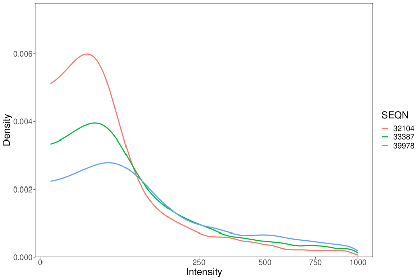
(b) Density curves.

Figure 1: Left plot: the trajectory of activity values during 7 consecutive days for a participant with subject ID 31131 in the physical monitor data. Right plot: Three medoid density curves by performing a $k$-medoid cluster algorithm with $k=3$. A square root transformation is performed on the x-axis.

In our analysis, we focus on white male subjects of age 20–50. We follow the similar pre-processing steps described in Lin et al. (2021) to deal with the observations of intensity values. First, we exclude observations whose reliability is questionable following NHANES protocol. Then for every subject, we remove the observations with intensity values higher than 1000 or equal to 0. Lastly, we remove subjects whose remaining observations with intensity values are less than 100 or missing in any covariate. The sample size is 427 after the pre-processing.

The raw activity intensity profiles across different subjects are not aligned and thus generally incomparable. To address this problem, one may use their distribution functions to represent them. But these intensity distributions lie in a manifold space. Instead, we apply the kernel mean embedding (Muandet et al., 2017) with a Gaussian kernel to generate distribution representations in Hilbert space, as discussed in Remark 1. Hence eventually, the treatments $A$ are taken as the kernel mean embeddings of the intensity distributions. We follow the same procedures in Section 5.1, including the choices of kernels and tuning parameters, to obtain all the five estimators.

To provide a clear look at how different the estimated causal effects are provided by different estimators, we present the estimated BMI values for three representative density curves chosen by performing a cluster analysis using a $k$-medoid cluster algorithm with $k=3$ on the density curves in the dataset. Figure 1(b) shows three medoid density curves while Table 3 shows the corresponding fitted BMI values produced by different estimators for these three curves. All five estimators provide the same order of BMI values for these three curves, indicating that a more active person tends to have a lower BMI. The result of NPFCBPS is rather similar to that of NW, while CFB, REG and FCBPS are more similar, and show a greater difference in BMI values between the curve with ID 33387 and 32104.

Next we study the performances of the five methods in categorizing the level of obesity in terms of the BMI value. According to the US Centers for Disease Control and Prevention, in terms of the BMI value, an adult may be categorized as: underweight (BMI $\leq 18.5$), healthy ($18.5<$ BMI $\leq 25$), overweight ($25<$ BMI $\leq 30$) and obese (BMI $>30$). We combine the underweight and healthy categories in our dataset because it only has three underweight observations. We visualize every unique activity profiles and their estimated BMI values ($\hat{\tau}(A)$) in Figure 2. For a better visualization, we stratify the collection of curves by the estimated BMI categories. NW and NPFCBPS categorize almost all the subjects as either overweight or obese. Moreover, the results of NW are counter-intuitive since there are clearly two subgroups within the designated obese group, with one subgroup of individuals whose activities are strenuous. The results of CFB are similar to those of REG and FCBPS, all indicating a steady and inverse relationship between strenuous activities and BMI.

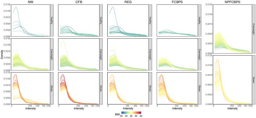
Figure 2: Density curves divided into different categories by their corresponding estimated BMI values using different estimators (NW, CFB, REG, FCBPS and NPFCBPS). A square root transformation is performed on the x-axis.

Table 3: Estimated BMI values for the three representative density curves in Figure 1(b) by different estimators. SEQN indicates the respondent sequence number, i.e., subject ID.

SEQN	CFB	FCBPS	NPFCBPS	REG	NW
33387	27.53	29.01	28.80	28.48	28.84
32104	30.72	31.62	30.28	31.37	29.30
39978	26.11	27.14	27.59	26.87	26.60

6 Discussion

In this paper, we establish a novel covariate balancing framework for FTE estimation. Our framework adopts the highly flexible weight-modified kernel ridge regression to characterize the FTE on the outcome. The proposed weights are obtained by balancing an RKHS of the functional treatment and can be computed efficiently. The proposed FTE estimator is guaranteed to achieve the optimal rate of convergence without any smoothness assumptions of the oracle weight function. Its appealing empirical performance is demonstrated in an extensive simulation study and a real data application.

In the following, we outline several directions for future work. Assumption 1 can be restrictive in practice as it requires all the covariates $\bm{X}$ that adjust the dependence between $\{Y(a),a\in\mathcal{A}\}$ and $A$ are observed. However, this is often not guaranteed in practice, which leads to the presence of unmeasured confounding. Inspired by the recent development in causal inference that tackles unmeasured confounding using instrumental or proxy variables, we will investigate FTE estimation while relaxing Assumption 1 to allow for unmeasured confounding. In addition, while Theorem 3 provides a convergence result for $\hat{\tau}$ with respect to the empirical norm, there are fundamental difficulties in calculating the $\mathcal{L}_{2}$ norm for functions with functional inputs numerically, and obtaining the $\mathcal{L}_{2}$ norm convergence rate. Obtaining such results probably requires a modification of our method to smooth the weights in order to establish the convergence of the estimated weight function.

Appendix A Algorithm

Input: Observed confounders $\bm{X}_{i}\in\mathbb{R}^{p}$ and approximated treatments $\hat{A}_{i}\in\mathcal{A}$, $i=1,\dots,n$; smoothing parameter $\lambda>0$; the fitted outcome regression model $\hat{m}$ and a sequence of tuning parameters $\eta_{k}$, $k=1,\dots,K$.

1 Calculate $\bm{G}_{A}$, $\bm{G}_{X}$, $\bar{\bm{G}}$ and $\bar{g}_{X}$ according to (13).

2 Decompose $\bm{G}_{F}$ and obtain $\bm{M}_{1}$, $\bm{M}_{2}$ and $\bm{M}$. for $k=1,\dots,K$ do

3       Optimize (16) by L-BFGS-B algorithm with $\eta=\eta_{k}$ and obtain solution $\hat{\bm{w}}^{(\eta_{k})}$.

4       Compute the value of $V(\eta_{k})$ from (17).

5 end for

6Select $\tilde{\eta}$ such that $V(\tilde{\eta})$ is the smallest among all $V(\eta_{k})$, $k=1,\dots,K$.

7Construct the adjusted response $Z_{i}=\hat{w}^{(\tilde{\eta})}_{i}Y_{i}$, $i=1,\dots,n$.

8Fix the response as $Z_{i}$, $i=1,\dots,n$ and obtain

$$\hat{\tau}=\left(\frac{1}{n}\sum_{i=1}^{n}\mathcal{S}_{\hat{A}_{i}}+\lambda\mathcal{I}\right)^{-1}\left(\frac{1}{n}\sum_{i=1}^{n}\mathcal{K}_{\hat{A}_{i}}Z_{i}\right).$$

Output: $\hat{\bm{w}}^{\tilde{\eta}}$ and $\hat{\tau}$.

9

Algorithm 1 Outlines for obtaining $\hat{\tau}$.

Appendix B Proof

Proof of Proposition 1.

Given the discussion of Assumptions in Section 4, under Assumption 5, the spectral theorem gives

$$\mathcal{S}=\sum_{l=1}^{L}t_{l}\langle\cdot,e_{l}\rangle_{{\mathcal{H}}_{A}}e_{l},$$

where $0<t_{l+1}\leq t_{l}$, $\{e_{l}\}_{l=1}^{\infty}$ is a basis of $\mathrm{Ker}\mathcal{\mathcal{S}}^{\perp}$. Define the operator $T:\mathcal{L}_{2}(\rho_{A})\rightarrow\mathcal{L}_{2}(\rho_{A})$ to be the integral operator of kernel $K_{A}$,

$$(T\rho)(a)=\mathbb{E}K_{A}(a,A)\psi(A)=\int_{\mathcal{A}}K_{A}(a,a^{\prime})\psi(a^{\prime})d\rho_{A}(a^{\prime})$$

for $\psi\in\mathcal{L}_{2}(\rho_{A})$. Based on Remark 2 in Caponnetto and De Vito (2007), it can be shown that

$$T=\sum_{l=1}^{K}\nu^{A}_{l}\langle\cdot,\phi^{A}_{l}\rangle_{\rho_{A}}\phi_{l}^{A},$$

where $\{\phi^{A}_{l}\}_{l=1}^{L}$ is basis of $\mathrm{Ker}T^{\perp}$, $T^{1/2}\phi^{A}_{l}=t_{l}^{1/2}\phi^{A}_{l}=e_{l}$ and $\lambda_{A}^{l}=t_{l}$, $l=1,\dots,L$. And we have

$$K_{A}(a_{1},a_{2})=\sum_{l=1}^{L}\nu^{A}_{l}\phi_{l}^{A}(a_{1})\phi^{A}_{l}(a_{2}).$$

As $K_{X}$ is a bounded continuous positive definite kernel, Mercer Theorem yields

$$K_{X}(\bm{x}_{1},\bm{x}_{2})=\sum_{l=1}^{L}\nu^{X}_{l}\phi^{X}_{l}(\bm{x}_{1})\phi^{X}_{l}(\bm{x}_{2}),$$

where $0<\phi_{l+1}^{X}\leq\phi^{X}_{l}$ are eigenvalues, $\{(\phi^{X}_{l}\}_{l=1}^{\infty}$ is a set of orthonormal basis in $\mathcal{L}_{2}(\rho_{X})$ and $\{(\nu^{X}_{l})^{1/2}\phi^{X}_{l}\}_{l=1}^{\infty}$ is a set of orthonormal basis in ${\mathcal{H}}_{X}$.

Next, we prove the direction that $\mathbb{E}_{\bm{X}\sim\rho_{X}}g(\cdot,\bm{X})\in{\mathcal{H}}_{A}$ for any $g\in{\mathcal{H}}$.

Given these two sets of basis, for any function $g\in{\mathcal{H}}$, it can be expressed as

$$g(a,\bm{x})=\sum_{l_{1},l_{2}}\beta_{l_{1},l_{2}}\sqrt{\nu_{l_{1}}^{A}}\sqrt{\nu_{l_{2}}^{X}}\phi^{A}_{l}(a)\phi^{X}_{l}(\bm{x}),$$

for some coefficients $\{\beta_{l_{1},l_{2}}\}_{l_{1},l_{2}=1}^{\infty}$ with

$$\|g\|^{2}_{{\mathcal{H}}}=\sum_{l_{1},l_{2}}\beta_{l_{1},l_{2}}^{2}<\infty.$$

Then we have

$$\|\mathbb{E}_{\bm{X}\sim\rho_{X}}g(\cdot,\bm{X})\|^{2}_{{\mathcal{H}}_{A}}=\sum_{l_{1}}(\beta_{l_{1},l_{2}})^{2}\left\{\mathbb{E}\left(\sum_{l_{2}}\sqrt{\nu_{l_{2}}^{X}}\phi_{l_{2}}^{X}(\bm{X})\right)\right\}^{2}\leq\sum_{l_{1}}(\beta_{l_{1},l_{2}})^{2}\mathbb{E}\left(\sum_{l_{2}}\sqrt{\nu_{l_{2}}^{X}}\phi_{l_{2}}^{X}(\bm{X})\right)^{2}$$

$$\leq\sum_{l_{1}}(\beta_{l_{1},l_{2}})^{2}\sum_{l_{2}}\nu_{l_{2}}^{X}(\beta_{l_{2}}^{X})^{2}\leq\left(\max_{l_{2}}\nu_{l_{2}}^{X}\right)\sum_{l_{1}}\sum_{l_{2}}(\beta^{A}_{l_{1},l_{2}})^{2}=\nu_{1}^{X}(\sum_{l_{1},l_{2}}\beta_{l_{1},l_{2}}^{2})=\nu_{1}^{X}\|g\|^{2}_{{\mathcal{H}}},$$

the second inequality is due to the fact that $\{\phi^{X}_{l}\}_{l=1}^{\infty}$ is orthonormal in $\mathcal{L}_{2}(\rho_{X})$. Note that $K_{X}$ is bounded, thus $\nu_{1}^{X}$ is bounded. The conclusion follows.

Now, we prove the direction that for any function $f\in{\mathcal{H}}_{A}$, there exists a function $g\in{\mathcal{H}}$, such that $\mathbb{E}_{\bm{X}\sim\rho_{X}}g(\cdot,\bm{X})\in{\mathcal{H}}$.

First, note that these exists a function $u\in{\mathcal{H}}_{X}$, such that

$$\mathbb{E}u(\bm{X})=\int_{\bm{x}}u(\bm{x})\rho_{X}(\bm{x})d\bm{x}\neq 0.$$

Take

$$g(a,\bm{x})=f(a)\frac{u(\bm{x})}{\mathbb{E}u(\bm{X})}.$$

One can verify that $\mathbb{E}_{\bm{X}\sim\rho_{X}}g(\cdot,\bm{X})=f(\cdot)$. Since ${\mathcal{H}}={\mathcal{H}}_{A}\otimes{\mathcal{H}}_{X}$, $f\in{\mathcal{H}}_{A}$ and ${u(\bm{x})}/{\mathbb{E}u(\bm{X})}\in{\mathcal{H}}_{X}$, therefore $g\in{\mathcal{H}}$. Therefore, the conclusion is verified. ∎

Proof of Theorem 1.

Take ${\mathcal{H}}_{n}^{\perp}$ as the orthogonal space of ${\mathcal{H}}_{n}$. For any function $u\in{\mathcal{H}}$, we can decompose it into two orthogonal parts $u_{1}$ and $u_{2}$ such that $u_{1}\in{\mathcal{H}}_{n}$ and $u_{2}\in{\mathcal{H}}_{n}^{\perp}$. Then for any $u\in{\mathcal{H}}$,

$$Q(\bm{w},\lambda,u)$$

$$=\frac{1}{n}\sum_{k=1}^{n}\left[\left\{\left(\frac{1}{n}\sum_{i=1}^{n}\mathcal{S}_{\hat{A}_{i}}+\lambda\mathcal{I}\right)^{-1}\left(\frac{1}{n}\sum_{i=1}^{n}\mathcal{K}_{\hat{A}_{i}}w_{i}u(\hat{A}_{i},\bm{X}_{i})\right)\right\}(A_{k})-\frac{1}{n}\sum_{j=1}^{n}u(A_{k},\bm{X}_{j})\right]^{2}$$

$$=\frac{1}{n}\sum_{k=1}^{n}\left[\left\{\left(\frac{1}{n}\sum_{i=1}^{n}\mathcal{S}_{\hat{A}_{i}}+\lambda\mathcal{I}\right)^{-1}\left(\frac{1}{n}\sum_{i=1}^{n}\mathcal{K}_{\hat{A}_{i}}w_{i}\langle K((\hat{A}_{i},\bm{X}_{i}),(\cdot,\cdot)),u\rangle\right)\right\}(A_{k})\right.$$

$$\left.-\frac{1}{n}\sum_{j=1}^{n}\langle K(\hat{A}_{k},\bm{X}_{j}),(\cdot,\cdot)),u\rangle\right]^{2}$$

$$= \frac{1}{n}\sum_{k=1}^{n}\left[\left\{\left(\frac{1}{n}\sum_{i=1}^{n}\mathcal{S}_{\hat{A}_{i}}+\lambda\mathcal{I}\right)^{-1}\left(\frac{1}{n}\sum_{i=1}^{n}\mathcal{K}_{\hat{A}_{i}}w_{i}\langle K_{A}(\cdot,\hat{A}_{i})K_{X}(\cdot,\bm{X}_{i}),(\cdot,\cdot)),u_{1}+u_{2}\rangle\right)\right\}(A_{k})\right.$$

$$\left.-\left\langle K_{A}(\cdot,\hat{A}_{k})\left\{\frac{1}{n}\sum_{j=1}^{n}K_{X}(\cdot,\bm{X}_{j})\right\},(\cdot,\cdot)),u_{1}+u_{2}\right\rangle\right]^{2}$$

$$=\frac{1}{n}\sum_{k=1}^{n}\left[\left\{\left(\frac{1}{n}\sum_{i=1}^{n}\mathcal{S}_{\hat{A}_{i}}+\lambda\mathcal{I}\right)^{-1}\left(\frac{1}{n}\sum_{i=1}^{n}\mathcal{K}_{\hat{A}_{i}}w_{i}\langle K_{A}(\cdot,\hat{A}_{i})K_{X}(\cdot,\bm{X}_{i}),(\cdot,\cdot)),u_{1}\rangle\right)\right\}(A_{k})\right.$$

$$\left.-\left\langle K_{A}(\cdot,\hat{A}_{k})\left\{\frac{1}{n}\sum_{j=1}^{n}K_{X}(\cdot,\bm{X}_{j})\right\},(\cdot,\cdot)),u_{1}\right\rangle\right]^{2}=Q(\bm{w},\lambda,u_{1}).$$

On the other hand, $\|u\|_{\mathcal{H}}=\|u_{1}\|_{\mathcal{H}}+\|u_{2}\|_{\mathcal{H}}$. For any $u$ such that $\|u\|_{\mathcal{H}}=1$ and $\|u_{1}\|_{{\mathcal{H}}}>0$, we can always find another $\tilde{u}=\frac{\|u\|_{\mathcal{H}}}{\|u_{1}\|_{\mathcal{H}}}u_{1}\in{\mathcal{H}}_{n}$. It is easy to verify that $\|\tilde{u}\|_{{\mathcal{H}}}=1$ and

$$Q(\bm{w},\lambda,\tilde{u})= Q\left(\bm{w},\lambda,\frac{\|u\|_{\mathcal{H}}}{\|u_{1}\|_{\mathcal{H}}}u_{1}\right)=\left(\frac{\|u\|_{\mathcal{H}}}{\|u_{1}\|_{\mathcal{H}}}\right)^{2}Q\left(\bm{w},\lambda,u_{1}\right)=\left(\frac{\|u\|_{\mathcal{H}}}{\|u_{1}\|_{\mathcal{H}}}\right)^{2}Q\left(\bm{w},\lambda,u\right)\geq Q\left(\bm{w},\lambda,u\right).$$

The conclusion follows. ∎

Proof of Lemma 1.

Consider any vectors $\bm{w}_{1}\in\mathbb{R}^{n}$ and $\bm{w}_{2}\in\mathbb{R}^{n}$, and $t\in[0,1]$. For $\bm{\beta}\in\mathbb{R}^{q}$, we have

$$\left\|\left[\bm{A}\mathrm{diag}\{t\bm{w}_{1}+(1-t)\bm{w}_{2}\}\bm{B}-\bm{D}\right]\bm{\beta}\right\|_{2}^{2}$$

$$= \left\|t\left[\bm{A}\mathrm{diag}(\bm{w}_{1})\bm{B}-\bm{D}\right]\bm{\beta}+(1-t)\left[\bm{A}\mathrm{diag}(\bm{w}_{2})\bm{B}-\bm{D}\right]\bm{\beta}\right\|_{2}^{2}$$

$$\leq t\left\|\left[\bm{A}\mathrm{diag}(\bm{w}_{1})\bm{B}-\bm{D}\right]\bm{\beta}\right\|_{2}^{2}+(1-t)\left\|\left[\bm{A}\mathrm{diag}(\bm{w}_{2})\bm{B}-\bm{D}\right]\bm{\beta}\right\|_{2}^{2}.$$

The inequality is due to the convexity of $\|\cdot\|_{2}^{2}$. Suppose that $\bm{\beta}$ is the right singular vector of $\bm{A}\mathrm{diag}\{t\bm{w}_{1}+(1-t)\bm{w}_{2}\}\bm{B}-\bm{D}$ that corresponds to the largest singular value. Then

$$\left[\sigma_{\max}\left\{\bm{A}\mathrm{diag}(\bm{w})\bm{B}-\bm{D}\right\}\right]^{2}$$

$$=\left\|\left[\bm{A}\mathrm{diag}\{t\bm{w}_{1}+(1-t)\bm{w}_{2}\}\bm{B}-\bm{D}\right]\bm{\beta}\right\|_{2}^{2}$$

$$\leq t\left\|\left[\bm{A}\mathrm{diag}(\bm{w}_{1})\bm{B}-\bm{D}\right]\bm{\beta}\right\|_{2}^{2}+(1-t)\left\|\left[\bm{A}\mathrm{diag}(\bm{w}_{2})\bm{B}-\bm{D}\right]\bm{\beta}\right\|_{2}^{2}$$

$$\leq t\left[\sigma_{\max}\left\{\bm{A}\mathrm{diag}(\bm{w})\bm{B}-\bm{D}\right\}\right]^{2}+(1-t)\left[\sigma_{\max}\left\{\bm{A}\mathrm{diag}(\bm{w}_{2})\bm{B}-\bm{D}\right\}\right]^{2}.$$

The second inequality is due to the definition of the largest singular value. Then conclusion follows. ∎

Proof of Theorem 2.

First, we derive the bounds for $\sup_{u\in{\mathcal{H}}(1)}Q(\bm{w^{*}},\lambda,u)$ and $R(\bm{w^{*}},\lambda)$

Take the function $z(a;u)=\mathbb{E}_{\bm{X}\sim\rho_{X}}u(a,X)$ for $u\in{\mathcal{H}}(1)$. Take $\mathcal{S}_{A}=\frac{1}{n}\sum_{i=1}^{n}\mathcal{S}_{A_{i}}$, $\mathcal{S}_{\hat{A}}=\frac{1}{n}\sum_{i=1}^{n}\mathcal{S}_{\hat{A}_{i}}$. It’s easy to see that $\sup_{u\in{\mathcal{H}}(1)}Q(w,\lambda,u)$ can be bounded by the following components:

$$\sup_{u\in{\mathcal{H}}(1)}Q(\bm{w^{*}},\lambda,u)$$

$$\lesssim\sup_{u\in{\mathcal{H}}(1)}\left\|\left(\frac{1}{n}\sum_{i=1}^{n}\mathcal{S}_{\hat{A}_{i}}+\lambda\mathcal{I}\right)^{-1}\left[\frac{1}{n}\sum_{i=1}^{n}\left(\mathcal{K}_{\hat{A}_{i}}\left\{w^{*}_{i}u(\hat{A}_{i},\bm{X}_{i})-z(\hat{A}_{i};u)\right\}\right.\right.\right.$$

$$\qquad\left.\left.\left.-\mathcal{K}_{A_{i}}\left\{w^{*}_{i}u(A_{i},\bm{X}_{i})-z(A_{i};u)\right\}\right)\right]\right\|_{n}^{2}$$ (22)

$$+\sup_{u\in{\mathcal{H}}(1)}\left\|\left(\mathcal{S}_{\hat{A}}+\lambda\mathcal{I}\right)^{-1}\left(\frac{1}{n}\sum_{i=1}^{n}\mathcal{S}_{A_{i}}-\frac{1}{n}\sum_{i=1}^{n}\mathcal{S}_{\hat{A}_{i}}\right)\left(\mathcal{S}_{A}+\lambda\mathcal{I}\right)^{-1}\right.$$

$$\qquad\left.\left[\frac{1}{n}\sum_{i=1}^{n}\mathcal{K}_{A_{i}}\left\{w^{*}_{i}u(A_{i},\bm{X}_{i})-z(A_{i};u)\right\}\right]\right\|_{n}^{2}$$ (23)

$$+\sup_{u\in{\mathcal{H}}(1)}\left\|\left(\frac{1}{n}\sum_{i=1}^{n}\mathcal{S}_{A_{i}}+\lambda\mathcal{I}\right)^{-1}\left[\frac{1}{n}\sum_{i=1}^{n}\mathcal{K}_{A_{i}}\left\{w^{*}_{i}u(A_{i},\bm{X}_{i})-z(A_{i};u)\right\}\right]\right\|_{n}^{2}$$ (24)

$$+\sup_{u\in{\mathcal{H}}(1)}\left\|\left(\frac{1}{n}\sum_{i=1}^{n}\mathcal{S}_{A_{i}}+\lambda\mathcal{I}\right)^{-1}\left[\frac{1}{n}\sum_{i=1}^{n}\mathcal{K}_{A_{i}}z(A_{i};u)\right]-z(\cdot;u)\right\|_{n}^{2}$$ (25)

$$+\sup_{u\in{\mathcal{H}}(1)}\left\|z(\cdot;u)-\frac{1}{n}\sum_{j=1}^{n}u(\cdot,\bm{X}_{j})\right\|_{n}^{2}$$ (26)

Next, we consider to bound (22), (23), (24), (25) and (26) one by one. Note that under the fully observed case (Assumption 6 1), $\hat{A}_{i}=A_{i}$ for $i=1,\dots,n$, and we only need to focus on (24) - (26).

First, follow the proof in Section A.1.11 of Szabó et al. (2015), by Assumption 6, we have

$$\left\|\left(\frac{1}{n}\sum_{i=1}^{n}\mathcal{S}_{\hat{A}_{i}}\right)-\left(\frac{1}{n}\sum_{i=1}^{n}\mathcal{S}_{A_{i}}\right)\right\|^{2}_{\mathcal{L}_{{\mathcal{H}}_{A}}}\leq\frac{1}{n}\sum_{i=1}^{n}\left\|\mathcal{S}_{\hat{A}_{i}}-\mathcal{S}_{A_{i}}\right\|^{2}_{\mathcal{L}_{{\mathcal{H}}_{A}}}=\mathop{}\mathopen{}\mathcal{O}\mathopen{}_{\mathrm{p}}\left({H^{2}C_{\ref*{cnt:kernelbound}}^{h}\kappa^{2h}}\right).$$

And note that for any function $f\in{\mathcal{H}}_{A}$,

$$\|f\|^{2}_{n}=\left\|\left(\frac{1}{n}\sum_{i=1}^{n}\mathcal{S}_{\hat{A}_{i}}\right)^{1/2}f\right\|^{2}_{{\mathcal{H}}_{A}}.$$

• For (22).

  $$\eqref{eqn:comp-1}$$

  $$\leq\left\|\left(\frac{1}{n}\sum_{i=1}^{n}\mathcal{S}_{\hat{A}_{i}}\right)^{1/2}\left(\frac{1}{n}\sum_{i=1}^{n}\mathcal{S}_{\hat{A}_{i}}+\lambda\mathcal{I}\right)^{-1}\right\|^{2}_{\mathcal{L}_{{\mathcal{H}}_{A}}}$$

  $$\qquad\times\left\|\frac{1}{n}\sum_{i=1}^{n}\left(\mathcal{K}_{\hat{A}_{i}}\left\{w^{*}_{i}u(\hat{A}_{i},\bm{X}_{i})-z(\hat{A}_{i};u)\right\}-\mathcal{K}_{A_{i}}\left\{w^{*}_{i}u(A_{i},\bm{X}_{i})-z(A_{i};u)\right\}\right)\right\|_{{\mathcal{H}}_{A}}^{2}.$$

  By the spectral theorem,

  $$\left\|\left(\frac{1}{n}\sum_{i=1}^{n}\mathcal{S}_{\hat{A}_{i}}\right)^{1/2}\left(\frac{1}{n}\sum_{i=1}^{n}\mathcal{S}_{\hat{A}_{i}}+\lambda\mathcal{I}\right)^{-1}\right\|^{2}_{\mathcal{L}_{{\mathcal{H}}_{A}}}\leq\frac{1}{\lambda}.$$

  And by Hölder continuous in Assumption 6,

  $$\left\|\frac{1}{n}\sum_{i=1}^{n}\left(\mathcal{K}_{\hat{A}_{i}}\left\{w^{*}_{i}u(\hat{A}_{i},\bm{X}_{i})-z(\hat{A}_{i};u)\right\}-\mathcal{K}_{A_{i}}\left\{w^{*}_{i}u(A_{i},\bm{X}_{i})-z(A_{i};u)\right\}\right)\right\|_{{\mathcal{H}}_{A}}^{2}$$

  $$\lesssim \frac{H^{2}}{n}\sum_{i=1}^{n}\left[d(A_{i},\hat{A}_{i})^{2h}C_{\ref*{cnt:overlapupper}}^{2}C_{\ref*{cnt:kernelbound}}^{4}\right]=\mathop{}\mathopen{}\mathcal{O}\mathopen{}_{\mathrm{p}}\left({H^{2}C_{\ref*{cnt:overlapupper}}^{2}C_{\ref*{cnt:kernelbound}}^{4}}\kappa^{2h}\right).$$

  Then

  $$\eqref{eqn:comp-1}=\mathop{}\mathopen{}\mathcal{O}\mathopen{}_{\mathrm{p}}\left(\frac{H^{2}C_{\ref*{cnt:overlapupper}}^{2}C_{\ref*{cnt:kernelbound}}^{4}\kappa^{2h}}{\lambda}\right).$$

• For (23), by similar proof, we can show that

  $$\eqref{eqn:comp0}$$

  $$\leq\left\|\left(\frac{1}{n}\sum_{i=1}^{n}\mathcal{S}_{\hat{A}_{i}}\right)^{1/2}\left(\frac{1}{n}\sum_{i=1}^{n}\mathcal{S}_{\hat{A}_{i}}+\lambda\mathcal{I}\right)^{-1}\right\|^{2}_{\mathcal{L}_{{\mathcal{H}}_{A}}}\left\|\left(\frac{1}{n}\sum_{i=1}^{n}\mathcal{S}_{A_{i}}-\frac{1}{n}\sum_{i=1}^{n}\mathcal{S}_{\hat{A}_{i}}\right)\right\|^{2}_{\mathcal{L}_{{\mathcal{H}}_{A}}}$$

  $$\qquad\times\sup_{u\in{\mathcal{H}}(1)}\left\|\left(\mathcal{S}_{A}+\lambda\mathcal{I}\right)^{-1}\left[\frac{1}{n}\sum_{i=1}^{n}\mathcal{K}_{A_{i}}\left\{w^{*}_{i}u(A_{i},\bm{X}_{i})-z(A_{i};u)\right\}\right]\right\|_{{\mathcal{H}}_{A}}^{2}$$

  $$=\mathop{}\mathopen{}\mathcal{O}\mathopen{}_{\mathrm{p}}\left(\frac{H^{2}C_{\ref*{cnt:overlapupper}}^{2}C_{\ref*{cnt:kernelbound}}^{4}C_{\ref*{cnt:kernelbound}}^{h}\kappa^{2h}}{\lambda}\right)\frac{1}{\lambda}$$

  $$\qquad\times\sup_{u\in{\mathcal{H}}(1)}\left\|\left(\mathcal{S}_{A}+\lambda\mathcal{I}\right)^{-\frac{1}{2}}\left[\frac{1}{n}\sum_{i=1}^{n}\mathcal{K}_{A_{i}}\left\{w^{*}_{i}u(A_{i},\bm{X}_{i})-z(A_{i};u)\right\}\right]\right\|_{{\mathcal{H}}_{A}}^{2}.$$

  By later argument (see the proof for bounding (24)), we can prove that

  $$\sup_{u\in{\mathcal{H}}(1)}\left\|\left(\mathcal{S}_{A}+\lambda\mathcal{I}\right)^{-\frac{1}{2}}\left[\frac{1}{n}\sum_{i=1}^{n}\mathcal{K}_{A_{i}}\left\{w^{*}_{i}u(A_{i},\bm{X}_{i})-z(A_{i};u)\right\}\right]\right\|_{{\mathcal{H}}_{A}}^{2}=\mathop{}\mathopen{}\mathcal{O}\mathopen{}_{\mathrm{p}}\left(\frac{\mathcal{N}(\lambda)}{n}\right).$$

  Then by the condition $\kappa^{2h}=\mathop{}\mathopen{}\mathcal{O}\mathopen{}(\lambda^{2})$, we have

  $$\eqref{eqn:comp0}=\mathop{}\mathopen{}\mathcal{O}\mathopen{}_{\mathrm{p}}\left(\frac{H^{2}C_{\ref*{cnt:overlapupper}}^{2}C_{\ref*{cnt:kernelbound}}^{4}C_{\ref*{cnt:kernelbound}}^{h}\kappa^{2h}}{\lambda}\frac{\mathcal{N}(\lambda)}{n\lambda}\right)=\mathop{}\mathopen{}\mathcal{O}\mathopen{}_{\mathrm{p}}\left(\frac{\mathcal{N}(\lambda)}{n}\right).$$

• Next, we focus on controlling term (24).

  We have

  $$\sup_{u\in{\mathcal{H}}(1)}\left\|\left(\frac{1}{n}\sum_{i=1}^{n}\mathcal{S}_{A_{i}}+\lambda\mathcal{I}\right)^{-1}\left[\frac{1}{n}\sum_{i=1}^{n}\mathcal{K}_{A_{i}}\left\{w^{*}_{i}u(A_{i},\bm{X}_{i})-z(A_{i};u)\right\}\right]\right\|_{n}^{2}$$

  $$=\sup_{u\in{\mathcal{H}}(1)}\left\|\left(\frac{1}{n}\sum_{i=1}^{n}\mathcal{S}_{\hat{A}_{i}}\right)^{1/2}\left(\frac{1}{n}\sum_{i=1}^{n}\mathcal{S}_{A_{i}}+\lambda\mathcal{I}\right)^{-1}\left[\frac{1}{n}\sum_{i=1}^{n}\mathcal{K}_{A_{i}}\left\{w^{*}_{i}u(A_{i},\bm{X}_{i})-z(A_{i};u)\right\}\right]\right\|^{2}_{{\mathcal{H}}_{A}}$$

  $$\leq\left\|\left(\frac{1}{n}\sum_{i=1}^{n}\mathcal{S}_{\hat{A}_{i}}\right)^{1/2}\left(\frac{1}{n}\sum_{i=1}^{n}\mathcal{S}_{A_{i}}+\lambda\mathcal{I}\right)^{-1}(\mathcal{S}+\lambda)^{\frac{1}{2}}\right\|^{2}_{\mathcal{L}({\mathcal{H}}_{A})}$$

  $$\qquad\times\sup_{u\in{\mathcal{H}}(1)}\left\|(\mathcal{S}+\lambda)^{-\frac{1}{2}}\left[\frac{1}{n}\sum_{i=1}^{n}\mathcal{K}_{A_{i}}\left\{w^{*}_{i}u(A_{i},\bm{X}_{i})-z(A_{i};u)\right\}\right]\right\|^{2}_{{\mathcal{H}}_{A}}.$$ (27)

  We start with bounding the first term:

  $$\left\|\left(\frac{1}{n}\sum_{i=1}^{n}\mathcal{S}_{\hat{A}_{i}}\right)^{\frac{1}{2}}(S_{\bm{A}}+\lambda\mathcal{I})^{-1}(S+\lambda\mathcal{I})^{\frac{1}{2}}\right\|_{\mathcal{L}({\mathcal{H}}_{A})}$$

  $$= \left\|\left(\frac{1}{n}\sum_{i=1}^{n}\mathcal{S}_{\hat{A}_{i}}\right)^{\frac{1}{2}}\left(\mathcal{S}+\lambda\mathcal{I}\right)^{-\frac{1}{2}}\left\{I-\left(\mathcal{S}+\lambda\mathcal{I}\right)^{-\frac{1}{2}}\left(\mathcal{S}-\left(\frac{1}{n}\sum_{i=1}^{n}\mathcal{S}_{A_{i}}\right)\right)\left(\mathcal{S}+\lambda\mathcal{I}\right)^{\frac{1}{2}}\right\}^{-1}\right\|_{\mathcal{L}({\mathcal{H}}_{A})}$$

  $$\leq \left\|\left(\frac{1}{n}\sum_{i=1}^{n}\mathcal{S}_{\hat{A}_{i}}\right)^{\frac{1}{2}}\left(\mathcal{S}+\lambda\mathcal{I}\right)^{-\frac{1}{2}}\right\|_{\mathcal{L}({\mathcal{H}}_{A})}$$

  $$\qquad\times\left\|\left\{I-\left(\mathcal{S}+\lambda\mathcal{I}\right)^{-\frac{1}{2}}\left(\mathcal{S}-\left(\frac{1}{n}\sum_{i=1}^{n}\mathcal{S}_{A_{i}}\right)\right)\left(\mathcal{S}+\lambda\mathcal{I}\right)^{-\frac{1}{2}}\right\}^{-1}\right\|_{\mathcal{L}({\mathcal{H}}_{A})}.$$

  From Caponnetto and De Vito (2007), we can show that if $n\geq 2C_{\eta}\kappa\mathcal{N}(\lambda)/\lambda$, where $C_{\eta}=32\log^{2}(6/\eta)$, and $\lambda\leq\|\mathcal{S}\|_{\mathcal{L}({\mathcal{H}}_{A})}$,

  $$\left\|\left(\mathcal{S}+\lambda\mathcal{I}\right)^{-\frac{1}{2}}\left(\mathcal{S}-\left(\frac{1}{n}\sum_{i=1}^{n}\mathcal{S}_{A_{i}}\right)\right)\left(\mathcal{S}+\lambda\mathcal{I}\right)^{-\frac{1}{2}}\right\|_{\mathcal{L}({\mathcal{H}}_{A})}\leq\frac{1}{2},$$ (28)

  with probability at least $1-2\eta/3$. And therefore under the same condition, we have

  $$\left\|\left\{I-\left(\mathcal{S}+\lambda\mathcal{I}\right)^{-\frac{1}{2}}\left(\mathcal{S}-\left(\frac{1}{n}\sum_{i=1}^{n}\mathcal{S}_{A_{i}}\right)\right)\left(\mathcal{S}+\lambda\mathcal{I}\right)^{-\frac{1}{2}}\right\}^{-1}\right\|_{\mathcal{L}({\mathcal{H}}_{A})}\leq 2.$$ (29)

  with probability at least $1-2\eta/3$.

  Then we bound $\|(\sum_{i=1}^{n}\mathcal{S}_{\hat{A}_{i}}/n)^{1/2}\left(\mathcal{S}+\lambda\mathcal{I}\right)^{-1/2}\|_{\mathcal{L}({\mathcal{H}}_{A})}$. Notice that

  $$\left\|\left(\frac{1}{n}\sum_{i=1}^{n}\mathcal{S}_{\hat{A}_{i}}\right)^{\frac{1}{2}}\left(\mathcal{S}+\lambda\mathcal{I}\right)^{-\frac{1}{2}}\right\|^{2}_{\mathcal{L}({\mathcal{H}}_{A})}=\left\|\left(\mathcal{S}+\lambda\mathcal{I}\right)^{-\frac{1}{2}}\left(\frac{1}{n}\sum_{i=1}^{n}\mathcal{S}_{\hat{A}_{i}}\right)\left(\mathcal{S}+\lambda\mathcal{I}\right)^{-\frac{1}{2}}\right\|_{\mathcal{L}({\mathcal{H}}_{A})}$$

  $$\leq\left\|\left(\mathcal{S}+\lambda\mathcal{I}\right)^{-\frac{1}{2}}\mathcal{S}\left(\mathcal{S}+\lambda\mathcal{I}\right)^{-\frac{1}{2}}\right\|_{\mathcal{L}({\mathcal{H}}_{A})}+\left\|\left(\mathcal{S}+\lambda\mathcal{I}\right)^{-\frac{1}{2}}\left(\mathcal{S}-\frac{1}{n}\sum_{i=1}^{n}\mathcal{S}_{\hat{A}_{i}}\right)\left(\mathcal{S}+\lambda\mathcal{I}\right)^{-\frac{1}{2}}\right\|_{\mathcal{L}({\mathcal{H}}_{A})}$$

  $$=\left\|\mathcal{S}^{\frac{1}{2}}\left(\mathcal{S}+\lambda\mathcal{I}\right)^{-\frac{1}{2}}\right\|^{2}_{\mathcal{L}({\mathcal{H}}_{A})}+\left\|\left(\mathcal{S}+\lambda\mathcal{I}\right)^{-\frac{1}{2}}\left(\mathcal{S}-\frac{1}{n}\sum_{i=1}^{n}\mathcal{S}_{\hat{A}_{i}}\right)\left(\mathcal{S}+\lambda\mathcal{I}\right)^{-\frac{1}{2}}\right\|_{\mathcal{L}({\mathcal{H}}_{A})}$$

  For the first component, it’s easy to see that

  $$\left\|\left(\mathcal{S}+\lambda\mathcal{I}\right)^{-\frac{1}{2}}\mathcal{S}\left(\mathcal{S}+\lambda\mathcal{I}\right)^{-\frac{1}{2}}\right\|_{\mathcal{L}({\mathcal{H}}_{A})}=\left\|\mathcal{S}^{\frac{1}{2}}\left(\mathcal{S}+\lambda\mathcal{I}\right)^{-\frac{1}{2}}\right\|^{2}_{\mathcal{L}({\mathcal{H}}_{A})}\leq 1$$

  because of the spectral theorem.

  And by (28), we have

  $$\left\|\left(\mathcal{S}+\lambda\mathcal{I}\right)^{-\frac{1}{2}}\left(\mathcal{S}-\frac{1}{n}\sum_{i=1}^{n}\mathcal{S}_{\hat{A}_{i}}\right)\left(\mathcal{S}+\lambda\mathcal{I}\right)^{-\frac{1}{2}}\right\|_{\mathcal{L}({\mathcal{H}}_{A})}$$

  $$\leq \left\|\left(\mathcal{S}+\lambda\mathcal{I}\right)^{-\frac{1}{2}}\left(\mathcal{S}-\frac{1}{n}\sum_{i=1}^{n}\mathcal{S}_{A_{i}}\right)\left(\mathcal{S}+\lambda\mathcal{I}\right)^{-\frac{1}{2}}\right\|_{\mathcal{L}({\mathcal{H}}_{A})}$$

  $$\qquad+\left\|\left(\mathcal{S}+\lambda\mathcal{I}\right)^{-\frac{1}{2}}\left(\frac{1}{n}\sum_{i=1}^{n}\mathcal{S}_{\hat{A}_{i}}-\frac{1}{n}\sum_{i=1}^{n}\mathcal{S}_{A_{i}}\right)\left(\mathcal{S}+\lambda\mathcal{I}\right)^{-\frac{1}{2}}\right\|_{\mathcal{L}({\mathcal{H}}_{A})}$$

  $$\leq \mathop{}\mathopen{}\mathcal{O}\mathopen{}_{\mathrm{p}}(1)+\frac{1}{\lambda}\mathop{}\mathopen{}\mathcal{O}\mathopen{}_{\mathrm{p}}\left({HC_{\ref*{cnt:kernelbound}}^{h/2}\kappa^{h}}\right)\leq\mathop{}\mathopen{}\mathcal{O}\mathopen{}_{\mathrm{p}}(1).$$

  The last inequality is due to the condition for $\kappa$ that $\kappa^{h}=\mathop{}\mathopen{}\mathcal{O}\mathopen{}(\lambda)$.

  Then we have

  $$\left\|\left(\frac{1}{n}\sum_{i=1}^{n}\mathcal{S}_{\hat{A}_{i}}\right)^{\frac{1}{2}}\left(\mathcal{S}+\lambda\mathcal{I}\right)^{-\frac{1}{2}}\right\|^{2}_{\mathcal{L}({\mathcal{H}}_{A})}=\mathop{}\mathopen{}\mathcal{O}\mathopen{}_{\mathrm{p}}\left(1\right).$$

  And overall we show that

  $$\left\|\left(\frac{1}{n}\sum_{i=1}^{n}\mathcal{S}_{\hat{A}_{i}}\right)^{\frac{1}{2}}(S_{\bm{A}}+\lambda\mathcal{I})^{-1}(S+\lambda\mathcal{I})^{\frac{1}{2}}\right\|_{\mathcal{L}({\mathcal{H}}_{A})}=\mathop{}\mathopen{}\mathcal{O}\mathopen{}_{\mathrm{p}}\left(1\right).$$ (30)

  Next, we bound the second term in (27). Take $r_{i}$ as independent Rademacher random variables. It’s easy to see that $\mathbb{E}\{w^{*}_{i}u(A_{i},X_{i})-z(A_{i};u)\}=0$ for every $i$ and $u\in{\mathcal{H}}(1)$. Due to symmetrization inequality, we have

  $$\mathbb{E}\sup_{u\in{\mathcal{H}}(1)}\left\|(\mathcal{S}+\lambda\mathcal{I})^{-1/2}\left[\frac{1}{n}\sum_{i=1}^{n}\mathcal{K}_{A_{i}}\left\{w^{*}_{i}u(A_{i},\bm{X}_{i})-z(A_{i};u)\right\}\right]\right\|^{2}_{{\mathcal{H}}_{A}}$$

  $$\leq 4\mathbb{E}\sup_{u\in{\mathcal{H}}(1)}\left\|(\mathcal{S}+\lambda\mathcal{I})^{1/2}\frac{1}{n}\sum_{i=1}^{n}K_{A_{i}}\{r_{i}w^{*}_{i}u(A_{i},\bm{X}_{i})\}\right\|^{2}_{{\mathcal{H}}_{A}}$$

  $$\qquad\qquad\qquad+4\mathbb{E}\sup_{u\in{\mathcal{H}}(1)}\left\|(\mathcal{S}+\lambda\mathcal{I})^{1/2}\frac{1}{n}\sum_{i=1}^{n}K_{A_{i}}r_{i}z(A_{i};u)\right\|^{2}_{{\mathcal{H}}_{A}}$$ (31)

  Let’s focus on the first term in (31).

  $$\mathbb{E}\sup_{u\in{\mathcal{H}}(1)}\left\|(\mathcal{S}+\lambda\mathcal{I})^{1/2}\frac{1}{n}\sum_{i=1}^{n}\mathcal{K}_{A_{i}}\{r_{i}w^{*}_{i}u(A_{i},\bm{X}_{i})\}\right\|^{2}_{{\mathcal{H}}_{A}}$$

  $$= \mathbb{E}\sup_{u\in{\mathcal{H}}(1)}\left\langle(\mathcal{S}+\lambda\mathcal{I})^{-1/2}\frac{1}{n}\sum_{i=1}^{n}\mathcal{K}_{A_{i}}\{r_{i}w^{*}_{i}u(A_{i},\bm{X}_{i})\},\right.$$

  $$\qquad\qquad\qquad\qquad\left.(\mathcal{S}+\lambda\mathcal{I})^{-1/2}\frac{1}{n}\sum_{i=1}^{n}\mathcal{K}_{A_{i}}\{r_{i}w^{*}_{i}u(A_{i},\bm{X}_{i})\}\right\rangle_{{\mathcal{H}}_{A}}$$

  $$= \mathbb{E}\sup_{u\in{\mathcal{H}}(1)}\frac{1}{n^{2}}\sum_{i=1}^{n}\sum_{j=1}^{n}r_{i}r_{j}w^{*}_{i}w^{*}_{j}u(A_{i},\bm{X}_{i})u(A_{j},\bm{X}_{j})$$

  $$\qquad\qquad\qquad\times\left\langle(\mathcal{S}+\lambda\mathcal{I})^{-1/2}\mathcal{K}_{A_{i}},(\mathcal{S}+\lambda\mathcal{I})^{-1/2}\mathcal{K}_{A_{j}}\right\rangle_{{\mathcal{H}}_{A}}$$

  $$\leq \frac{1}{n^{2}}\mathbb{E}\sup_{u\in{\mathcal{H}}(1)}\sum_{i=1}^{n}(w^{*}_{i})^{2}u^{2}(A_{i},\bm{X}_{i})\left\langle(\mathcal{S}+\lambda\mathcal{I})^{-1/2}\mathcal{K}_{A_{i}},(\mathcal{S}+\lambda\mathcal{I})^{-1/2}\mathcal{K}_{A_{i}}\right\rangle_{{\mathcal{H}}_{A}}$$

  $$+ \frac{1}{n^{2}}\mathbb{E}\sup_{u\in{\mathcal{H}}(1)}\sum_{i\neq j}r_{i}r_{j}w^{*}_{i}w^{*}_{j}u(A_{i},\bm{X}_{i})u(A_{j},\bm{X}_{j})\left\langle(\mathcal{S}+\lambda\mathcal{I})^{-1/2}\mathcal{K}_{A_{i}},(\mathcal{S}+\lambda\mathcal{I})^{-1/2}\mathcal{K}_{A_{j}}\right\rangle_{{\mathcal{H}}_{A}}$$

  $$=(i)+(ii)$$ (32)

  We first deal with the (i). For every $u\in\mathcal{H}(1)$, $\|u\|_{\infty}=\sup_{(a,\bm{x})}|\langle K((a,\bm{x}),(\cdot,\cdot)),u\rangle_{{\mathcal{H}}}|\leq\sup_{(a,x)}|K((a,\bm{x}),(a,\bm{x}))|\leq C_{\ref*{cnt:kernelbound}}\kappa$. By contraction inequality and symmetrization inequality, we have

  $$\mathbb{E}\sup_{u\in{\mathcal{H}}(1)}\sum_{i=1}^{n}(w^{*}_{i})^{2}u^{2}(A_{i},\bm{X}_{i})\left\langle(\mathcal{S}+\lambda\mathcal{I})^{-1/2}\mathcal{K}_{A_{i}},(\mathcal{S}+\lambda\mathcal{I})^{-1/2}\mathcal{K}_{A_{i}}\right\rangle_{{\mathcal{H}}_{A}}$$

  $$\leq nC_{\ref*{cnt:kernelbound}}^{2}\kappa^{2}\mathbb{E}\left\langle(\mathcal{S}+\lambda\mathcal{I})^{-1/2}K_{A_{1}},(\mathcal{S}+\lambda\mathcal{I})^{-1/2}\mathcal{K}_{A_{1}}\right\rangle_{{\mathcal{H}}_{A}}$$

  $$\leq nC_{\ref*{cnt:kernelbound}}^{2}\kappa^{2}\mathbb{E}\|\mathcal{K}_{A_{1}}^{*}(\mathcal{S}+\lambda\mathcal{I})^{-1}\mathcal{K}_{A_{1}}\|_{\mathcal{L}({\mathcal{H}}_{A})}$$

  $$\leq nC_{\ref*{cnt:kernelbound}}^{2}\kappa^{2}\mathbb{E}\{\mbox{Tr}(\mathcal{K}_{A_{1}}^{*}(\mathcal{S}+\lambda\mathcal{I})^{-1}\mathcal{K}_{A_{1}})\}$$

  $$= nC_{\ref*{cnt:kernelbound}}^{2}\kappa^{2}\mathbb{E}\{\mbox{Tr}((\mathcal{S}+\lambda\mathcal{I})^{-1}\mathcal{K}_{A_{1}}\mathcal{K}_{A_{1}}^{*})\}=nC_{\ref*{cnt:kernelbound}}^{2}\kappa^{2}\int_{a}\mbox{Tr}\left\{(\mathcal{S}+\lambda\mathcal{I})^{-1}\mathcal{S}_{a}\right\}d\rho_{A}(a)$$

  $$\leq nC_{\ref*{cnt:kernelbound}}^{2}\kappa^{2}\mbox{Tr}\left\{(\mathcal{S}+\lambda\mathcal{I})^{-1}\mathcal{S}\right\}=nC_{\ref*{cnt:kernelbound}}^{2}\kappa^{2}\mathcal{N}(\lambda).$$

  Next, we study the term (ii). Based on the proof in Proposition 1, we have $K_{A}(\cdot,\cdot)=\sum_{l_{1}=1}^{\infty}\nu_{l_{1}}^{A}\phi_{l_{1}}^{A}(\cdot)\phi_{l_{1}}^{A}(\cdot)$, where $\nu_{l_{1}}^{A}$ are eigenvalues and $\phi_{l_{1}}^{A}(\cdot)$ are eigenfunctions (orthonormal basis of $\mathcal{L}_{2}(\rho_{A})$). $K_{X}(\cdot,\cdot)=\sum_{l_{2}=1}^{\infty}\nu_{l_{2}}^{X}\phi_{l_{2}}^{X}(\cdot)\phi_{l_{2}}^{X}(\cdot)$, where $\nu_{l_{2}}^{X}$ are eigenvalues and $\phi_{l_{2}}^{X}(\cdot)$ are eigenfunctions (orthonormal basis of $\mathcal{L}_{2}(\rho_{X})$. Since the reproducing kernel for ${\mathcal{H}}$ is $K((\cdot,\star),(\cdot,\star))=K_{A}(\cdot,\cdot)K_{X}(\star,\star)$, we have $K((\cdot,\star),(\cdot,\star))=\sum_{l=1}^{\infty}\nu_{l}\phi_{l}(\cdot,\star)\phi_{l}(\cdot,\star)$, where $\nu_{l}=\nu_{l_{1}}^{A}\nu_{l_{2}}^{X}$ and $\phi_{l}(\cdot,\star)=\phi_{l_{1}}^{A}(\cdot)\phi_{l_{2}}^{X}(\star)$ for some $l_{1},l_{2}$ such that $\nu$, $l=1,\dots,\infty$ is nonincreasing. Take $\Phi(\cdot,\star)=\{\sqrt{\nu}\phi_{l}(\cdot,\star)\}_{l=1}^{\infty}$. ${\mathcal{H}}(1)=\{u(\cdot,\star)=\langle\beta,\Phi(\cdot,\star)\rangle:\sum_{l=1}^{\infty}\beta^{2}_{l}\leq 1\}$. Take $\mathcal{E}(1)=\{\beta:\sum_{l=1}^{\infty}\beta^{2}_{l}\leq 1\}$, then

  $$(ii)\leq\mathbb{E}\sup_{\beta\in\mathcal{E}(1)}\left\{\sum_{l=1}^{\infty}(\beta_{l})^{2}\sum_{l^{\prime}=1}^{\infty}(\beta_{l^{\prime}})^{2}\right\}^{\frac{1}{2}}$$

  $$\leq \left[\sum_{l=1}^{\infty}\sum_{l^{\prime}=1}^{\infty}\sum_{i\neq j}\mathbb{E}\left\langle(\mathcal{S}+\lambda\mathcal{I})^{-\frac{1}{2}}\mathcal{K}_{A_{i}},(\mathcal{S}+\lambda\mathcal{I})^{-\frac{1}{2}}\mathcal{K}_{A_{j}}\right\rangle_{{\mathcal{H}}_{A}}^{2}(w^{*}_{i})^{2}(w^{*}_{j})^{2}\nu_{l}\phi^{2}_{l}(A_{i},\bm{X}_{i})\nu_{l^{\prime}}\phi^{2}_{l^{\prime}}(A_{j},\bm{X}_{j})\right]^{\frac{1}{2}}$$

  $$\leq \left[\sum_{l=1}^{\infty}\sum_{l^{\prime}=1}^{\infty}\sum_{i\neq j}\mathbb{E}\left\{(w_{i}^{*})^{2}\left\langle(\mathcal{S}+\lambda\mathcal{I})^{-\frac{1}{2}}K_{A_{i}},(\mathcal{S}+\lambda\mathcal{I})^{-\frac{1}{2}}K_{A_{i}}\right\rangle_{{\mathcal{H}}_{A}}\nu_{l}\phi_{l}^{2}(A_{i},\bm{X}_{i})\right\}\right.$$

  $$\left.\mathbb{E}\left\{(w_{j}^{*})^{2}\left\langle(\mathcal{S}+\lambda\mathcal{I})^{-\frac{1}{2}}K_{A_{j}},(\mathcal{S}+\lambda\mathcal{I})^{-\frac{1}{2}}K_{A_{j}}\right\rangle_{{\mathcal{H}}_{A}}\nu_{l^{\prime}}\phi_{l^{\prime}}^{2}(A_{j},\bm{X}_{j})\right\}\right]^{\frac{1}{2}}$$

  $$= \left[\sum_{i\neq j}\mathbb{E}\left\{(w_{i}^{*})^{2}\left\langle(\mathcal{S}+\lambda\mathcal{I})^{-\frac{1}{2}}K_{A_{i}},(\mathcal{S}+\lambda\mathcal{I})^{-\frac{1}{2}}K_{A_{i}}\right\rangle_{{\mathcal{H}}_{A}}\left(\sum_{l=1}^{\infty}\nu_{l}\phi_{l}^{2}(A_{i},\bm{X}_{i})\right)\right\}\right.$$

  $$\left.\mathbb{E}\left\{(w_{j}^{*})^{2}\left\langle(\mathcal{S}+\lambda\mathcal{I})^{-\frac{1}{2}}K_{A_{j}},(\mathcal{S}+\lambda\mathcal{I})^{-\frac{1}{2}}K_{A_{j}}\right\rangle_{{\mathcal{H}}_{A}}\left(\sum_{l^{\prime}=1}^{\infty}\nu_{l^{\prime}}\phi_{l^{\prime}}^{2}(A_{j},\bm{X}_{j})\right)\right\}\right]^{\frac{1}{2}}.$$

  The first inequality by adopting Cauchy Schwarz inequality. The second inequality is due to that $r_{i},\ i=1,\dots,n$ are all independent Rademacher random variables. The third inequality is because that $(A_{i},X_{i}),\ i=1,\dots,n$ are independent pairs and

  $$\left\langle(\mathcal{S}+\lambda\mathcal{I})^{-1/2}\mathcal{K}_{A_{i}},(\mathcal{S}+\lambda\mathcal{I})^{-1/2}\mathcal{K}_{A_{j}}\right\rangle_{{\mathcal{H}}_{A}}^{2}$$

  $$\leq \left\langle(\mathcal{S}+\lambda\mathcal{I})^{-1/2}\mathcal{K}_{A_{i}},(\mathcal{S}+\lambda\mathcal{I})^{-1/2}\mathcal{K}_{A_{i}}\right\rangle_{{\mathcal{H}}_{A}}\left\langle(\mathcal{S}+\lambda\mathcal{I})^{-1/2}\mathcal{K}_{A_{j}},(\mathcal{S}+\lambda\mathcal{I})^{-1/2}\mathcal{K}_{A_{j}}\right\rangle_{{\mathcal{H}}_{A}}$$

  Note that

  $$\sum_{l=1}^{\infty}\nu_{l}\phi_{l}^{2}(A_{i},\bm{X}_{i})=K_{A}(A_{i},A_{i})K_{X}(\bm{X}_{i},\bm{X}_{i})\leq\kappa C_{\ref*{cnt:kernelbound}}.$$

  Then

  $$\mathbb{E}\left\{(w_{i}^{*})^{2}\left\langle(\mathcal{S}+\lambda\mathcal{I})^{-1/2}K_{A_{i}},(\mathcal{S}+\lambda\mathcal{I})^{-1/2}K_{A_{i}}\right\rangle_{{\mathcal{H}}_{A}}\left(\sum_{l=1}^{\infty}\nu_{l}\phi_{l}^{2}(A_{i},X_{i})\right)\right\}$$

  $$\leq C_{\ref*{cnt:overlapupper}}^{2}\kappa C_{\ref*{cnt:kernelbound}}\mathbb{E}\left\langle(\mathcal{S}+\lambda\mathcal{I})^{-1/2}K_{A_{i}},(\mathcal{S}+\lambda\mathcal{I})^{-1/2}K_{A_{i}}\right\rangle_{{\mathcal{H}}_{A}}$$

  $$\leq C_{\ref*{cnt:overlapupper}}^{2}\kappa C_{\ref*{cnt:kernelbound}}\mathcal{N}(\lambda)$$

  Now we prove that

  $$(ii)\leq\frac{C_{\ref*{cnt:overlapupper}}^{2}\kappa C_{\ref*{cnt:kernelbound}}}{n^{2}}\left\{\sqrt{n(n-1)}\mathcal{N}(\lambda)\right\}\leq\frac{C_{\ref*{cnt:overlapupper}}^{2}\kappa C_{\ref*{cnt:kernelbound}}}{n}\mathcal{N}(\lambda).$$

  Combine the bound of $(i)$ and $(ii)$ into (32), we have

  $$\mathbb{E}\sup_{u\in{\mathcal{H}}(1)}\left\|(\mathcal{S}+\lambda\mathcal{I})^{1/2}\frac{1}{n}\sum_{i=1}^{n}\mathcal{K}_{A_{i}}\{r_{i}w^{*}_{i}u(A_{i},\bm{X}_{i})\}\right\|^{2}_{{\mathcal{H}}_{A}}\leq\frac{C_{\ref*{cnt:kernelbound}}^{2}\kappa^{2}\mathcal{N}(\lambda)}{n}+\frac{C_{\ref*{cnt:overlapupper}}^{2}\kappa C_{\ref*{cnt:kernelbound}}}{n}\mathcal{N}(\lambda)$$ (33)

  Next we deal with the second term in (31). For $u\in{\mathcal{H}}(1)$, by previous construction of ${\mathcal{H}}(1)$, we can express $u(a,x)=\sum_{l_{1}}\sum_{l_{2}}\beta^{A}_{l_{1}}\beta^{X}_{l_{2}}\sqrt{\nu^{A}_{l_{1}}\nu^{X}_{l_{2}}}\phi_{l_{1}}^{A}(a)\phi_{l_{2}}^{X}(x)$ for some coefficients $\beta^{A}_{l_{1}}$ and $\beta^{X}_{l_{2}}$. Then

  $$\|z(\cdot;u)\|^{2}_{{\mathcal{H}}_{A}} =\sum_{l_{1}}(\beta^{A}_{l_{1}})^{2}\left\{\mathbb{E}\left(\sum_{l_{2}}\sqrt{\nu_{l_{2}}^{X}}\beta^{X}_{l_{2}}\phi_{l_{2}}^{X}(\bm{X})\right)\right\}^{2}\leq\sum_{l_{1}}(\beta^{A}_{l_{1}})^{2}\mathbb{E}\left(\sum_{l_{2}}\sqrt{\nu_{l_{2}}^{X}}\beta^{X}_{l_{2}}\phi_{l_{2}}^{X}(\bm{X})\right)^{2}$$

  $$\leq\sum_{l_{1}}(\beta^{A}_{l_{1}})^{2}\sum_{l_{2}}\nu_{l_{2}}^{X}(\beta_{l_{2}}^{X})^{2}\leq\left(\max_{l_{2}}\nu_{l_{2}}^{X}\right)\sum_{l_{1}}\sum_{l_{2}}(\beta^{A}_{l_{1}})^{2}(\beta_{l_{2}}^{X})^{2}=\nu_{1}^{X}$$

  Then $\{z(\cdot;u):\|u\|_{\mathcal{H}}\leq 1\}\subset\{z:\|z\|_{{\mathcal{H}}_{A}}\leq\nu_{1}^{X}\}$, we can follow previous strategy and prove that

  $$\mathbb{E}\sup_{u\in{\mathcal{H}}(1)}\left\|(\mathcal{S}+\lambda\mathcal{I})^{1/2}\frac{1}{n}\sum_{i=1}^{n}K_{A_{i}}r_{i}z(A_{i};u)\right\|^{2}_{{\mathcal{H}}_{A}}$$ (34)

  $$\leq(\nu_{1}^{X})^{2}\mathbb{E}\sup_{z\in\{z:\|z\|_{{\mathcal{H}}_{A}}\leq 1\}}\left\|(\mathcal{S}+\lambda\mathcal{I})^{1/2}\frac{1}{n}\sum_{i=1}^{n}K_{A_{i}}r_{i}z(A_{i})\right\|^{2}_{{\mathcal{H}}_{A}}$$

  $$\leq\frac{(\nu_{1}^{X})^{2}\kappa^{2}\mathcal{N}(\lambda)}{n}+\frac{(\nu_{1}^{X})^{2}C_{\ref*{cnt:overlapupper}}^{2}\kappa}{n}\mathcal{N}(\lambda)$$

  And overall, there exists a constant $c_{1}\ltx@label{cnt:exp_{L}2_{b}ound}>0$ depending on $\nu_{1}^{X},\kappa,C_{\ref*{cnt:overlapupper}},C_{\ref*{cnt:kernelbound}}$, such that

  $$\mathbb{E}\sup_{u\in{\mathcal{H}}(1)}\left\|(\mathcal{S}+\lambda\mathcal{I})^{-1/2}\left[\frac{1}{n}\sum_{i=1}^{n}\mathcal{K}_{A_{i}}\left\{w^{*}_{i}u(A_{i},\bm{X}_{i})-z(A_{i};u)\right\}\right]\right\|^{2}_{{\mathcal{H}}_{A}}\leq\frac{c_{\ref*{cnt:exp_L2_bound}}\mathcal{N}(\lambda)}{n}.$$

  And combine the result with (30), we have

  $$\sup_{u\in{\mathcal{H}}(1)}\left\|\left(\frac{1}{n}\sum_{i=1}^{n}\mathcal{S}_{A_{i}}+\lambda\mathcal{I}\right)^{-1}\left[\frac{1}{n}\sum_{i=1}^{n}\mathcal{K}_{A_{i}}\left\{w^{*}_{i}u(A_{i},\bm{X}_{i})-z(A_{i};u)\right\}\right]\right\|^{2}_{n}=\mathop{}\mathopen{}\mathcal{O}\mathopen{}_{\mathrm{p}}\left(\frac{\mathcal{N}(\lambda)}{n}\right).$$

• Next, we consider to bound (25). By the above arguments,

  $$\sup_{u\in{\mathcal{H}}(1)}\left\|\left(\frac{1}{n}\sum_{i=1}^{n}\mathcal{S}_{A_{i}}+\lambda\mathcal{I}\right)^{-1}\left[\frac{1}{n}\sum_{i=1}^{n}\mathcal{K}_{A_{i}}z(A_{i};u)\right]-z(\cdot;u)\right\|_{n}^{2}$$

  $$\leq \nu_{1}^{X}\sup_{z\in\{z:\|z\|_{{\mathcal{H}}_{A}}\leq 1\}}\left\|\left(\frac{1}{n}\sum_{i=1}^{n}\mathcal{S}_{A_{i}}+\lambda\mathcal{I}\right)^{-1}\left[\frac{1}{n}\sum_{i=1}^{n}\mathcal{K}_{A_{i}}z(A_{i})\right]-z\right\|_{n}^{2}$$

  Take $z^{\lambda}=(\mathcal{S}+\lambda\mathcal{I})^{-1}Sz$. We can verify that

  $$\|z^{\lambda}-z\|^{2}_{\mathcal{H}_{A}} =\left\|\left[(\mathcal{S}+\lambda\mathcal{I})^{-1}S-\mathcal{I}\right]z\right\|^{2}_{\mathcal{H}_{A}}=\sum_{l=1}^{\infty}\left[\frac{\nu_{l}^{A}}{\nu_{l}^{A}+\lambda}-1\right]^{2}\langle z,\phi_{l}^{A}\rangle_{\mathcal{H}_{A}}^{2}\leq\sum_{l=1}^{\infty}\langle z,\phi_{l}^{A}\rangle_{\mathcal{H}_{A}}^{2}=\|z\|_{\mathcal{H}_{A}}^{2}.$$

  $$\|z^{\lambda}-z\|^{2}_{\mathcal{L}_{2}({\rho_{A}})} =\left\|\sqrt{\mathcal{S}}\left[(\mathcal{S}+\lambda\mathcal{I})^{-1}S\right]z-z\right\|^{2}_{\mathcal{H}_{A}}=\sum_{l=1}^{\infty}\nu_{l}^{A}\left[\frac{\nu_{l}^{A}}{\nu_{l}^{A}+\lambda}-1\right]^{2}\langle z,\phi_{l}^{A}\rangle_{\mathcal{H}_{A}}^{2}$$

  $$=\sum_{l=1}^{\infty}\left[\frac{\lambda}{\sqrt{\nu_{l}^{A}}+\lambda/\sqrt{\nu_{l}^{A}}}\right]^{2}\langle z,\phi_{l}^{A}\rangle_{\mathcal{H}_{A}}^{2}\leq\sum_{l=1}^{\infty}\left(\frac{\lambda}{\sqrt{2\lambda}}\right)^{2}\langle z,\phi_{l}^{A}\rangle_{\mathcal{H}_{A}}^{2}=\lambda/2\|z\|_{\mathcal{H}_{A}}^{2}.$$

  Next, we derive the bound for

  $$\sup_{z\in\{z:\|z\|_{{\mathcal{H}}_{A}}\leq 1\}}\|z^{\lambda}-z\|_{n}^{2}.$$

  Take $z^{\prime}=z^{\lambda}-z$, given that $\|z^{\prime}\|_{{\mathcal{H}}_{A}}\leq\sqrt{c_{2}\ltx@label{cnt:zhnorm}}\|z\|_{{\mathcal{H}}_{A}}\leq\sqrt{c_{\ref*{cnt:zhnorm}}}$ and $\|z^{\prime}\|_{\mathcal{L}_{2}(\rho_{A})}\leq\sqrt{c_{\ref*{cnt:zl2norm}}\lambda}\|z\|_{{\mathcal{H}}_{A}}\leq\sqrt{c_{3}\ltx@label{cnt:zl2norm}\lambda}$ for some positive constants $c_{\ref*{cnt:zhnorm}}$ and $c_{\ref*{cnt:zl2norm}}$. Follow the same proof of Lemma 42 in Mendelson (2002), we can show that the Rademacher complexity

  $$\mathbb{E}\sup_{z^{\prime}\in\{z:\|z\|_{{\mathcal{H}}_{A}}\leq\sqrt{c_{\ref*{cnt:zhnorm}}},\|z\|_{\mathcal{L}_{2}(\rho_{A})}\leq\sqrt{c_{\ref*{cnt:zl2norm}}\lambda}\}}\left|\frac{1}{n}\sum_{i=1}^{n}r_{i}z^{\prime}(A_{i})\right|^{2}\leq\frac{c_{4}\ltx@label{cnt:emp_{r}ade}}{n}\left(\sum_{l=1}^{\infty}\min\{\nu^{A}_{l},\lambda\}\right)$$

  for some constant $c_{\ref*{cnt:emp_rade}}>0$ depending on $c_{\ref*{cnt:zhnorm}}$ and $c_{\ref*{cnt:zl2norm}}$. Next, we apply Corollary 2.2 in Bartlett et al. (2005), we can verify there exists a constant $b>0$ such that $\|z^{\prime}\|_{\infty}\leq b$ for any $\|z^{\prime}\|_{{\mathcal{H}}_{A}}\leq\sqrt{c_{\ref*{cnt:zhnorm}}}$. Then for any $x>0$, if $\lambda\geq 10b\{{c_{\ref*{cnt:emp_rade}}}\sum_{l=1}^{\infty}\min\{\nu^{A}_{l},\lambda\}/n\}^{1/2}+11b^{2}x/n$, we have

  $$\{z^{\prime}\in\{z:\|z\|_{{\mathcal{H}}_{A}}\leq\sqrt{c_{\ref*{cnt:zhnorm}}}\}:\|z^{\prime}\|^{2}_{\mathcal{L}_{2}(\rho_{A})}\leq c_{\ref*{cnt:zl2norm}}\lambda\}\subseteq\{z^{\prime}\in\{z:\|z\|_{{\mathcal{H}}_{A}}\leq\sqrt{c_{\ref*{cnt:zhnorm}}}\}:\|z^{\prime}\|^{2}_{n}\leq 2c_{\ref*{cnt:zl2norm}}\lambda\},$$

  with probability at least $1-\exp(-x)$. Note that $v^{A}_{l}=t_{l}$, then as long as $\sqrt{\sum_{l=1}^{\infty}\min\{t_{l},\lambda\}}/(\sqrt{n}\lambda)=\mathop{}\mathopen{}\mathcal{O}\mathopen{}_{\mathrm{p}}(1)$, we have $\|z^{\prime}\|_{n}^{2}=\mathop{}\mathopen{}\mathcal{O}\mathopen{}_{\mathrm{p}}(\lambda)$. The above inequalities also holds for $\hat{A}_{i}$, $i=1,\dots,n$ as $\hat{A}_{i}$ are independent samples from $\mathcal{A}$. Then we have the following the inequality

  $$\sup_{z\in\{z:\|z\|_{{\mathcal{H}}_{A}}\leq 1\}}\left\|\left(\frac{1}{n}\sum_{i=1}^{n}\mathcal{S}_{A_{i}}+\lambda\mathcal{I}\right)^{-1}\left[\frac{1}{n}\sum_{i=1}^{n}\mathcal{K}_{A_{i}}z(A_{i})\right]-z\right\|_{n}^{2}$$

  $$\leq 2\sup_{z\in\{z:\|z\|_{{\mathcal{H}}_{A}}\leq 1\}}\left\|\left(\frac{1}{n}\sum_{i=1}^{n}\mathcal{S}_{A_{i}}+\lambda\mathcal{I}\right)^{-1}\left(\mathcal{S}-\frac{1}{n}\sum_{i=1}^{n}\mathcal{S}_{A_{i}}\right)\left(z^{\lambda}-z\right)\right\|_{n}^{2}$$

  $$+2\sup_{z\in\{z:\|z\|_{{\mathcal{H}}_{A}}\leq 1\}}\|z^{\lambda}-z\|^{2}_{n}$$

  $$\leq \left\|\left(\frac{1}{n}\sum_{i=1}^{n}\mathcal{S}_{\hat{A}_{i}}\right)^{1/2}\left(\frac{1}{n}\sum_{i=1}^{n}\mathcal{S}_{A_{i}}+\lambda\mathcal{I}\right)^{-1}(S+\lambda\mathcal{I})^{\frac{1}{2}}\right\|^{2}_{\mathcal{L}({\mathcal{H}}_{A})}$$

  $$\qquad c_{\ref*{cnt:zhnorm}}\sup_{v\in\{z:\|z\|_{{\mathcal{H}}_{A}}\leq 1\}}\left\|\left(\mathcal{S}+\lambda\mathcal{I}\right)^{-\frac{1}{2}}\left(\mathcal{S}-\frac{1}{n}\sum_{i=1}^{n}\mathcal{S}_{A_{i}}\right)v\right\|_{{\mathcal{H}}_{A}}^{2}+c_{\ref*{cnt:zl2norm}}\lambda$$ (35)

  The operator norm in (35) can be bounded via (30). It remains to bound

  $$\sup_{v\in\{z:\|z\|_{{\mathcal{H}}_{A}}\leq 1\}}\left\|\left(\mathcal{S}+\lambda\mathcal{I}\right)^{-\frac{1}{2}}\left(\mathcal{S}-\frac{1}{n}\sum_{i=1}^{n}\mathcal{S}_{A_{i}}\right)v\right\|^{2}_{{\mathcal{H}}_{A}}.$$

  Note that $\mathbb{E}\mathcal{S}_{A_{i}}=\mathcal{S}$, then we can apply the symmetrization equality again

  $$\sup_{v\in\{z:\|z\|_{{\mathcal{H}}_{A}}\leq 1\}}\left\|\left(\mathcal{S}+\lambda\mathcal{I}\right)^{-\frac{1}{2}}\left(\mathcal{S}-\frac{1}{n}\sum_{i=1}^{n}\mathcal{S}_{A_{i}}\right)v\right\|^{2}_{{\mathcal{H}}_{A}}\leq 4\mathbb{E}\sup_{v\in\{z:\|z\|_{{\mathcal{H}}_{A}}\leq 1\}}\left\|\left(\mathcal{S}+\lambda\mathcal{I}\right)^{-\frac{1}{2}}\frac{1}{n}\sum_{i=1}^{n}\mathcal{S}_{A_{i}}r_{i}v\right\|^{2}_{{\mathcal{H}}_{A}},$$

  where $r_{i}$, $i=1,\dots,n$ are independent Rademacher random variables.

  Follow the similar proof in proving term (24), we can show that

  $$\mathbb{E}\sup_{v\in\{z:\|z\|_{{\mathcal{H}}_{A}}\leq 1\}}\left\|\left(\mathcal{S}+\lambda\mathcal{I}\right)^{-\frac{1}{2}}\frac{1}{n}\sum_{i=1}^{n}\mathcal{S}_{A_{i}}r_{i}v\right\|^{2}_{{\mathcal{H}}_{A}}\leq c_{5}\ltx@label{cnt:rade2}\frac{\mathcal{N}(\lambda)}{n}$$

  for some constant $c_{\ref*{cnt:rade2}}>0$ depending on $\kappa$. And overall, we prove that

  $$\eqref{eqn:comp2}=\mathop{}\mathopen{}\mathcal{O}\mathopen{}_{\mathrm{p}}\left(\frac{\mathcal{N}(\lambda)}{n}+\lambda\right)$$

• Last, we bound the term (26). First, fixed any $a\in\mathcal{A}$, we derive the bound for $\mathbb{E}\sup_{u\in{\mathcal{H}}(1)}[z(a;u)-\sum_{j=1}^{n}u(a,\bm{X}_{j})/n]^{2}$.

  By symmetrization inequality, we have

  $$\mathbb{E}\sup_{u\in{\mathcal{H}}(1)}\left[z(a;u)-\frac{\sum_{j=1}^{n}u(a,\bm{X}_{j})}{n}\right]^{2}\leq 4\mathbb{E}\sup_{u\in{\mathcal{H}}(1)}\left[\frac{1}{n}\sum_{j=1}^{n}r_{j}u(a,\bm{X}_{j})\right]^{2}$$

  Again by previous construction of ${\mathcal{H}}(1)$, we have ${\mathcal{H}}(1)=\{u(\cdot,\star)=\langle\beta,\Phi(\cdot,\star)\rangle:\sum_{l=1}^{\infty}\beta^{2}_{l}\leq 1\}$. Take $\mathcal{E}(1)=\{\beta:\sum_{l=1}^{\infty}\beta^{2}_{l}\leq 1\}$.

  $$\mathbb{E}\sup_{u\in{\mathcal{H}}(1)}\left[\frac{1}{n}\sum_{j=1}^{n}r_{i}u(a,\bm{X}_{j})\right]^{2}\leq\mathbb{E}\sup_{\beta\in\mathcal{E}(1)}\left[\frac{1}{n}\sum_{j=1}^{n}r_{j}\left\{\sum_{l}\beta_{l}\sqrt{\nu_{l}}\phi_{l}(a,\bm{X}_{j})\right\}\right]^{2}$$

  $$\leq \mathbb{E}\sup_{\beta\in\mathcal{E}(1)}\left(\sum_{l}\beta_{l}^{2}\right)\left[\frac{1}{n}\sum_{j=1}^{n}r_{j}\sqrt{\nu_{l}}\phi_{l}(a,\bm{X}_{j})\right]^{2}\leq\sum_{l}\nu_{l}\mathbb{E}\left[\frac{1}{n}\sum_{j=1}^{n}r_{j}\phi_{l}(a,\bm{X}_{j})\right]^{2}\leq\frac{1}{n}\sum_{l}\nu_{l}\mathbb{E}\phi_{l}^{2}(a,\bm{X}_{1})$$

  $$= \frac{1}{n}K_{A}(a,a)\mathbb{E}K_{X}(\bm{X}_{1},\bm{X}_{1})\leq\frac{1}{n}\kappa C_{\ref*{cnt:kernelbound}}K_{A}(a,a).$$

  Then we can show that

  $$\mathbb{E}\left\{\sup_{u\in{\mathcal{H}}(1)}\left\|z(\cdot;u)-\frac{1}{n}\sum_{j=1}^{n}u(\cdot,\bm{X}_{j})\right\|_{n}^{2}\right\}\leq\mathbb{E}\left(\mathbb{E}\left\{\sup_{u\in{\mathcal{H}}(1)}\left[z(A;u)-\frac{1}{n}\sum_{j=1}^{n}u(A,\bm{X}_{j})\right]^{2}\mid A\right\}\right)$$

  $$\lesssim\frac{1}{n}\kappa K_{A}(A,A)\lesssim\frac{1}{n}=\mathop{}\mathopen{}\mathcal{O}\mathopen{}_{\mathrm{p}}\left(\frac{1}{\sqrt{n}}\right).$$

  Combine the bounds derived for (24), (25) and (26), the bound for $\sup_{u\in{\mathcal{H}}(1)}Q(w^{*},\lambda,\|\cdot\|_{n},u)$ follows.

  To bound the penalty term $R(w^{*},\lambda)$, note that

  $$R(\bm{w^{*}},\lambda,)=\frac{1}{n^{2}}\sum_{i=1}^{n}(w^{*}_{i})^{2}\left\|\left(\frac{1}{n}\sum_{i=1}^{n}\mathcal{S}_{\hat{A}_{i}}+\lambda\mathcal{I}\right)^{-1}\mathcal{K}_{\hat{A}_{i}}\right\|_{n}^{2}$$

  $$\leq\frac{C_{\ref*{cnt:overlapupper}}}{n^{2}}\sum_{i=1}^{n}\left\|\left(\frac{1}{n}\sum_{i=1}^{n}\mathcal{S}_{\hat{A}_{i}}+\lambda\mathcal{I}\right)^{-1}\mathcal{K}_{\hat{A}_{i}}\right\|_{n}^{2}$$

  $$\leq\frac{C_{\ref*{cnt:overlapupper}}}{n^{2}}\sum_{i=1}^{n}\left\|\left(\frac{1}{n}\sum_{i=1}^{n}\mathcal{S}_{\hat{A}_{i}}\right)^{1/2}\left(\frac{1}{n}\sum_{i=1}^{n}\mathcal{S}_{\hat{A}_{i}}+\lambda\mathcal{I}\right)^{-1}(\mathcal{S}+\lambda\mathcal{I})^{\frac{1}{2}}\right\|^{2}_{\mathcal{L}({\mathcal{H}}_{A})}\left\|(\mathcal{S}+\lambda\mathcal{I})^{-\frac{1}{2}}\mathcal{K}_{\hat{A}_{i}}\right\|^{2}_{{\mathcal{H}}_{A}}.$$

  $$\left\|\left(\frac{1}{n}\sum_{i=1}^{n}\mathcal{S}_{\hat{A}_{i}}\right)^{1/2}\left(\frac{1}{n}\sum_{i=1}^{n}\mathcal{S}_{\hat{A}_{i}}+\lambda\mathcal{I}\right)^{-1}(\mathcal{S}+\lambda\mathcal{I})^{\frac{1}{2}}\right\|_{\mathcal{L}({\mathcal{H}}_{A})}$$

  $$\leq \Bigg{\|}\left(\frac{1}{n}\sum_{i=1}^{n}\mathcal{S}_{\hat{A}_{i}}\right)^{1/2}\left(\frac{1}{n}\sum_{i=1}^{n}\mathcal{S}_{\hat{A}_{i}}+\lambda\mathcal{I}\right)^{-1}\left(\frac{1}{n}\sum_{i=1}^{n}\mathcal{S}_{\hat{A}_{i}}-\frac{1}{n}\sum_{i=1}^{n}\mathcal{S}_{A_{i}}\right)$$

  $$\qquad\qquad\qquad\times(\mathcal{S}_{\bm{A}}+\lambda\mathcal{I})^{-1}(\mathcal{S}+\lambda\mathcal{I})^{\frac{1}{2}}\Bigg{\|}_{\mathcal{L}({\mathcal{H}}_{A})}$$

  $$+\left\|\left(\frac{1}{n}\sum_{i=1}^{n}\mathcal{S}_{\hat{A}_{i}}\right)^{1/2}\left(\frac{1}{n}\sum_{i=1}^{n}\mathcal{S}_{A_{i}}+\lambda\mathcal{I}\right)^{-1}(\mathcal{S}+\lambda\mathcal{I})^{\frac{1}{2}}\right\|_{\mathcal{L}({\mathcal{H}}_{A})}$$

  $$=\mathop{}\mathopen{}\mathcal{O}\mathopen{}_{\mathrm{p}}(\lambda^{-1}\kappa^{h})+\mathop{}\mathopen{}\mathcal{O}\mathopen{}_{\mathrm{p}}(1)=\mathop{}\mathopen{}\mathcal{O}\mathopen{}_{\mathrm{p}}(1).$$

  The last two equalities are due to (30) and the condition of $\kappa$.

  $$\left\|(\mathcal{S}+\lambda\mathcal{I})^{-\frac{1}{2}}\mathcal{K}_{\hat{A}_{i}}\right\|^{2}_{{\mathcal{H}}_{A}}=\left\|(\mathcal{S}+\lambda\mathcal{I})^{-\frac{1}{2}}\left(\mathcal{S}_{\hat{A}_{i}}-\mathcal{S}_{A_{i}}\right)(\mathcal{S}+\lambda\mathcal{I})^{-\frac{1}{2}}\right\|_{\mathcal{L}({\mathcal{H}}_{A})}$$

  $$+\left\|(\mathcal{S}+\lambda\mathcal{I})^{-\frac{1}{2}}\mathcal{S}_{A_{i}}(\mathcal{S}+\lambda\mathcal{I})^{-\frac{1}{2}}\right\|_{\mathcal{L}({\mathcal{H}}_{A})}$$

  $$\leq\left\|\left(\mathcal{S}_{\hat{A}_{i}}-\mathcal{S}_{A_{i}}\right)(\mathcal{S}+\lambda\mathcal{I})^{-1}\right\|_{\mathcal{L}({\mathcal{H}}_{A})}+\left\|\mathcal{S}_{A_{i}}(\mathcal{S}+\lambda\mathcal{I})^{-1}\right\|_{\mathcal{L}({\mathcal{H}}_{A})}$$

  $$\leq\frac{1}{\lambda}\left\|\mathcal{S}_{\hat{A}_{i}}-\mathcal{S}_{A_{i}}\right\|_{\mathcal{L}({\mathcal{H}}_{A})}+\left\|\mathcal{S}_{A_{i}}(\mathcal{S}+\lambda\mathcal{I})^{-1}\right\|_{\mathcal{L}({\mathcal{H}}_{A})}$$

  It’s easy to verify that

  $$\mathbb{E}\|\mathcal{S}_{A_{i}}(\mathcal{S}+\lambda\mathcal{I})^{-1}\|_{\mathcal{L}({\mathcal{H}}_{A})}\leq\mathbb{E}\left\{\mbox{Tr}\left((\mathcal{S}+\lambda\mathcal{I})^{-1}\mathcal{K}_{A_{i}}\mathcal{K}_{A_{i}}^{*}\right)\right\}\leq\mbox{Tr}\{(\mathcal{S}+\lambda\mathcal{I})^{-1}\mathcal{S}\}=\mathcal{N}(\lambda).$$

  Then combine with all the bounds, we obtain

  $$R(\bm{w^{*}},\lambda)=\mathop{}\mathopen{}\mathcal{O}\mathopen{}_{\mathrm{p}}\left(\frac{\mathcal{N}(\lambda)}{n}\right)+\mathop{}\mathopen{}\mathcal{O}\mathopen{}_{\mathrm{p}}\left(\frac{\kappa^{h}}{\lambda}\right)\leq\mathop{}\mathopen{}\mathcal{O}\mathopen{}_{\mathrm{p}}\left(\frac{\mathcal{N}(\lambda)}{n}\right).$$

The last inequality is due to the condition of $\kappa$.

Now we are ready to bound $\sup_{u\in{\mathcal{H}}(1)}Q(\hat{\bm{w}},\lambda,u)$ and $R(\hat{\bm{w}},\lambda)$. Since $\bm{\hat{w}}$ is the solution of (12), by the basic inequality, we have

$$\sup_{u\in{\mathcal{H}}(1)}Q(\bm{\hat{w}},\lambda,u)+\eta R(\bm{\hat{w}},\lambda)\leq\sup_{u\in{\mathcal{H}}(1)}Q(\bm{w^{*}},\lambda,u)+\eta R(\bm{w^{*}},\lambda).$$

Therefore, we have

$$\sup_{u\in{\mathcal{H}}(1)}Q(\bm{\hat{w}},\lambda,u)\leq\left\{\sup_{u\in{\mathcal{H}}(1)}Q(\bm{w^{*}},\lambda,u)+\eta R(\bm{w^{*}},\lambda)\right\}=\mathop{}\mathopen{}\mathcal{O}\mathopen{}_{\mathrm{p}}\left[(1+\eta)\frac{\mathcal{N}(\lambda)}{n}+\lambda\right],$$

$$R(\bm{\hat{w}},\lambda)\leq\eta^{-1}\left\{\sup_{u\in{\mathcal{H}}(1)}Q(\bm{w^{*}},\lambda,u)+\eta R(\bm{w^{*}},\lambda)\right\}=\mathop{}\mathopen{}\mathcal{O}\mathopen{}_{\mathrm{p}}\left[\frac{\mathcal{N}(\lambda)}{n}+\eta^{-1}\left(\lambda+\frac{\mathcal{N}(\lambda)}{n}\right)\right].$$

∎

Proof of Theorem 3.

By Theorem 2, we can derive that

$$Q(\bm{\hat{w}},\lambda,m)=\mathop{}\mathopen{}\mathcal{O}\mathopen{}_{\mathrm{p}}\left[\|m\|^{2}_{{\mathcal{H}}}\left(\frac{\mathcal{N}(\lambda)}{n}+\lambda+\eta\frac{\mathcal{N}(\lambda)}{n}\right)\right],$$

$$R(\bm{\hat{w}},\lambda,)=\mathop{}\mathopen{}\mathcal{O}\mathopen{}_{\mathrm{p}}\left[\eta^{-1}\left(\frac{\mathcal{N}(\lambda)}{n}+\lambda\right)+\frac{\mathcal{N}(\lambda)}{n}\right].$$

From the decomposition, we have

$$\|\hat{\tau}-\tau\|_{n}= \left\|\left(\frac{1}{n}\sum_{i=1}^{n}\mathcal{S}_{\hat{A}_{i}}+\lambda\mathcal{I}\right)^{-1}\left(\frac{1}{n}\sum_{i=1}^{n}\mathcal{K}_{\hat{A}_{i}}\hat{w}_{i}Y_{i}\right)-\tau\right\|_{n}$$

$$= \left\|\left(\frac{1}{n}\sum_{i=1}^{n}\mathcal{S}_{\hat{A}_{i}}+\lambda\mathcal{I}\right)^{-1}\left(\frac{1}{n}\sum_{i=1}^{n}\mathcal{K}_{\hat{A}_{i}}\hat{w}_{i}m(\hat{A}_{i},\bm{X}_{i})\right)-\frac{1}{n}\sum_{j=1}^{n}m(\cdot,\bm{X}_{j})\right\|_{n}$$ (36)

$$+\left\|\frac{1}{n}\sum_{j=1}^{n}m(\cdot,\bm{X}_{j})-\tau\right\|_{n}$$ (37)

$$+\left\|\left(\frac{1}{n}\sum_{i=1}^{n}\mathcal{S}_{\hat{A}_{i}}+\lambda\mathcal{I}\right)^{-1}\left(\frac{1}{n}\sum_{i=1}^{n}\mathcal{K}_{\hat{A}_{i}}\hat{w}_{i}\epsilon_{i}\right)\right\|_{n}$$ (38)

$$\eqref{eqn:empnorm_decomp1}=\{Q(\bm{\hat{w}},\lambda,m)\}^{1/2}=\mathop{}\mathopen{}\mathcal{O}\mathopen{}_{\mathrm{p}}\left[\|m\|_{{\mathcal{H}}}\left(\frac{\mathcal{N}(\lambda)}{n}+\lambda+\eta\frac{\mathcal{N}(\lambda)}{n}\right)^{1/2}\right].$$

From the bound of (26) in Theorem 2, we have

$$\eqref{eqn:empnorm_decomp2}=\mathop{}\mathopen{}\mathcal{O}\mathopen{}_{\mathrm{p}}\left(\frac{\|m\|_{\mathcal{H}}}{\sqrt{n}}\right).$$

Notice that under Assumption 3,

$$\mathbb{E}\left\{\left\|\left(\frac{1}{n}\sum_{i=1}^{n}\mathcal{S}_{A_{i}}+\lambda\right)^{-1}\left(\frac{1}{n}\sum_{i=1}^{n}\mathcal{K}_{A_{i}}\hat{w}_{i}\epsilon_{i}\right)\right\|^{2}_{n}\mid A_{i},i=1,\dots,n\right\}$$

$$\leq\sigma_{0}^{2}R(\bm{\hat{w}},\lambda)=\sigma_{0}^{2}\mathop{}\mathopen{}\mathcal{O}\mathopen{}_{\mathrm{p}}\left[\eta^{-1}\left(\frac{\mathcal{N}(\lambda)}{n}+\lambda\right)+\frac{\mathcal{N}(\lambda)}{n}\right].$$

Then

$$\eqref{eqn:empnorm_decomp3}=\mathop{}\mathopen{}\mathcal{O}\mathopen{}_{\mathrm{p}}\left(\sigma_{0}\eta^{-1/2}\left(\frac{\mathcal{N}(\lambda)}{n}+\lambda\right)^{1/2}+\left(\frac{\mathcal{N}(\lambda)}{n}\right)^{1/2}\right).$$

Under Assumption 7 and the conditions of $\eta$ and $\lambda$ stated in Theorem 3, we note that $\mathcal{N}(\lambda)\asymp\lambda^{-1/b}$. Follow the proof of Lemma S7 in Wang et al. (2020), to satisfy the condition $\sqrt{\sum_{l=1}^{\infty}\min\{t_{l},\lambda\}/(n\lambda^{2})}=\mathop{}\mathopen{}\mathcal{O}\mathopen{}(1)$, we need $n\lambda^{-(1+1/b)}=\mathop{}\mathopen{}\mathcal{O}\mathopen{}(1)$, which is the same condition for $\mathcal{N}(\lambda)(\lambda n)^{-1}=\mathop{}\mathopen{}\mathcal{O}\mathopen{}(1)$. Then we can see that when $\lambda\asymp n^{-b/(1+b)}$, the conditions are satisfied and $\lambda\asymp(\mathcal{N}(\lambda)/\sqrt{n}$.

The bound of $\|\hat{\tau}-\tau\|_{n}$ follows.

∎

References

- Bahadori et al. (2022) Bahadori, T., E. T. Tchetgen, and D. Heckerman (2022). End-to-end balancing for causal continuous treatment-effect estimation. In International Conference on Machine Learning, pp. 1313–1326. PMLR.
- Bartlett et al. (2005) Bartlett, P. L., O. Bousquet, and S. Mendelson (2005). Local Rademacher complexities. The Annals of Statistics 33(4), 1497–1537.
- Caponnetto and De Vito (2007) Caponnetto, A. and E. De Vito (2007). Optimal rates for the regularized least-squares algorithm. Foundations of Computational Mathematics 7(3), 331–368.
- Ciarleglio et al. (2018) Ciarleglio, A., E. Petkova, T. Ogden, and T. Tarpey (2018). Constructing treatment decision rules based on scalar and functional predictors when moderators of treatment effect are unknown. Journal of the Royal Statistical Society: Series C (Applied Statistics) 67(5), 1331–1356.
- Delaigle and Hall (2010) Delaigle, A. and P. Hall (2010). Defining probability density for a distribution of random functions. The Annals of Statistics 38(2), 1171–1193.
- Ding and Li (2018) Ding, P. and F. Li (2018). Causal inference: a missing data perspective. Statistical Science 33(2), 214–237.
- Feng et al. (2012) Feng, P., X.-H. Zhou, Q.-M. Zou, M.-Y. Fan, and X.-S. Li (2012). Generalized propensity score for estimating the average treatment effect of multiple treatments. Statistics in Medicine 31(7), 681–697.
- Fong et al. (2018) Fong, C., C. Hazlett, and K. Imai (2018). Covariate balancing propensity score for a continuous treatment: Application to the efficacy of political advertisements. The Annals of Applied Statistics 12(1), 156–177.
- Fukumizu et al. (2009) Fukumizu, K., A. Gretton, G. Lanckriet, B. Schölkopf, and B. K. Sriperumbudur (2009). Kernel choice and classifiability for RKHS embeddings of probability distributions. Advances in Neural Information Processing Systems 22.
- Galvao and Wang (2015) Galvao, A. F. and L. Wang (2015). Uniformly semiparametric efficient estimation of treatment effects with a continuous treatment. Journal of the American Statistical Association 110(512), 1528–1542.
- Garreau et al. (2017) Garreau, D., W. Jitkrittum, and M. Kanagawa (2017). Large sample analysis of the median heuristic. arXiv preprint arXiv:1707.07269.
- Griggs (2013) Griggs, W. (2013). Penalized spline regression and its applications. Whitman College Report. Available online at: https://www. whitman. edu/Documents/Academics/Mathematics/Griggs. pdf.
- Hainmueller (2012) Hainmueller, J. (2012). Entropy balancing for causal effects: a multivariate reweighting method to produce balanced samples in observational studies. Political Analysis, 25–46.
- Hirano and Imbens (2004) Hirano, K. and G. W. Imbens (2004). The propensity score with continuous treatments. Applied Bayesian Modeling and Causal Inference from Incomplete-Data Perspectives 226164, 73–84.
- Hirano et al. (2003) Hirano, K., G. W. Imbens, and G. Ridder (2003). Efficient estimation of average treatment effects using the estimated propensity score. Econometrica 71(4), 1161–1189.
- Imai and Ratkovic (2014) Imai, K. and M. Ratkovic (2014). Covariate balancing propensity score. Journal of the Royal Statistical Society: Series B (Statistical Methodology), 243–263.
- Imai and van Dyk (2004) Imai, K. and D. A. van Dyk (2004). Causal inference with general treatment regimes: generalizing the propensity score. Journal of the American Statistical Association 99(467), 854–866.
- Imbens (2000) Imbens, G. W. (2000). The role of the propensity score in estimating dose-response functions. Biometrika 87(3), 706–710.
- Imbens (2004) Imbens, G. W. (2004). Nonparametric estimation of average treatment effects under exogeneity: a review. Review of Economics and Statistics 86(1), 4–29.
- Kadri et al. (2010) Kadri, H., E. Duflos, P. Preux, S. Canu, and M. Davy (2010). Nonlinear functional regression: a functional rkhs approach. In Proceedings of the Thirteenth International Conference on Artificial Intelligence and Statistics, pp. 374–380. JMLR Workshop and Conference Proceedings.
- Kadri et al. (2016) Kadri, H., E. Duflos, P. Preux, S. Canu, A. Rakotomamonjy, and J. Audiffren (2016). Operator-valued kernels for learning from functional response data. Journal of Machine Learning Research 17(20), 1–54.
- Kallus and Santacatterina (2019) Kallus, N. and M. Santacatterina (2019). Kernel optimal orthogonality weighting: A balancing approach to estimating effects of continuous treatments. arXiv preprint arXiv:1910.11972.
- Kennedy et al. (2017) Kennedy, E. H., Z. Ma, M. D. McHugh, and D. S. Small (2017). Non-parametric methods for doubly robust estimation of continuous treatment effects. Journal of the Royal Statistical Society: Series B (Statistical Methodology) 79(4), 1229–1245.
- Laber and Staicu (2018) Laber, E. B. and A.-M. Staicu (2018). Functional feature construction for individualized treatment regimes. Journal of the American Statistical Association 113(523), 1219–1227.
- Li (2019) Li, F. (2019). Propensity score weighting for causal inference with multiple treatments. The Annals of Applied Statistics 13(4), 2389–2415.
- Li et al. (2020) Li, Y., K. Kuang, B. Li, P. Cui, J. Tao, H. Yang, and F. Wu (2020). Continuous treatment effect estimation via generative adversarial de-confounding. In Proceedings of the 2020 KDD Workshop on Causal Discovery, pp. 4–22. PMLR.
- Lin et al. (2021) Lin, Z., D. Kong, and L. Wang (2021). Causal inference on distribution functions. arXiv preprint arXiv:2101.01599.
- Lopez and Gutman (2017) Lopez, M. J. and R. Gutman (2017). Estimation of causal effects with multiple treatments: a review and new ideas. Statistical Science, 432–454.
- McKeague and Qian (2014) McKeague, I. W. and M. Qian (2014). Estimation of treatment policies based on functional predictors. Statistica Sinica 24(3), 1461.
- Mendelson (2002) Mendelson, S. (2002). Geometric parameters of kernel machines. In International Conference on Computational Learning Theory, pp. 29–43. Springer.
- Miao et al. (2022) Miao, R., W. Xue, and X. Zhang (2022). Average treatment effect estimation in observational studies with functional covariates. Statistics and Its Interface 15(2), 237–246.
- Muandet et al. (2017) Muandet, K., K. Fukumizu, B. Sriperumbudur, and B. Schölkopf (2017). Kernel mean embedding of distributions: a review and beyond. Foundations and Trends® in Machine Learning 10(1-2), 1–141.
- Neovius et al. (2005) Neovius, M., Y. Linne, and S. Rossner (2005). BMI, waist-circumference and waist-hip-ratio as diagnostic tests for fatness in adolescents. International Journal of Obesity 29(2), 163–169.
- Oliva et al. (2015) Oliva, J., W. Neiswanger, B. Póczos, E. Xing, H. Trac, S. Ho, and J. Schneider (2015). Fast function to function regression. In Artificial Intelligence and Statistics, pp. 717–725. PMLR.
- Qin and Zhang (2007) Qin, J. and B. Zhang (2007). Empirical-likelihood-based inference in missing response problems and its application in observational studies. Journal of the Royal Statistical Society: Series B (Statistical Methodology) 69(1), 101–122.
- Raskutti et al. (2012) Raskutti, G., M. J Wainwright, and B. Yu (2012). Minimax-optimal rates for sparse additive models over kernel classes via convex programming. Journal of Machine Learning Research 13(2).
- Rice and Rosenblatt (1983) Rice, J. and M. Rosenblatt (1983). Smoothing splines: regression, derivatives and deconvolution. The Annals of Statistics, 141–156.
- Robins et al. (2000) Robins, J. M., M. A. Hernan, and B. Brumback (2000). Marginal structural models and causal inference in epidemiology. Epidemiology 11(5), 550–560.
- Rosenbaum et al. (2010) Rosenbaum, P. R., P. Rosenbaum, and Briskman (2010). Design of Observational Studies, Volume 10. Springer.
- Rosenbaum and Rubin (1983) Rosenbaum, P. R. and D. B. Rubin (1983). The central role of the propensity score in observational studies for causal effects. Biometrika 70(1), 41–55.
- Rubin (2007) Rubin, D. B. (2007). The design versus the analysis of observational studies for causal effects: parallels with the design of randomized trials. Statistics in Medicine 26(1), 20–36.
- Smale and Zhou (2007) Smale, S. and D.-X. Zhou (2007). Learning theory estimates via integral operators and their approximations. Constructive Approximation 26(2), 153–172.
- Stuart (2010) Stuart, E. A. (2010). Matching methods for causal inference: A review and a look forward. Statistical Science 25(1), 1–21.
- Szabó et al. (2015) Szabó, Z., A. Gretton, B. Póczos, and B. Sriperumbudur (2015). Two-stage sampled learning theory on distributions. In Artificial Intelligence and Statistics, pp. 948–957. PMLR.
- Szabó et al. (2016) Szabó, Z., B. K. Sriperumbudur, B. Póczos, and A. Gretton (2016). Learning theory for distribution regression. Journal of Machine Learning Research 17(1), 5272–5311.
- Tan et al. (2022) Tan, R., W. Huang, Z. Zhang, and G. Yin (2022). Causal effect of functional treatment. arXiv preprint arXiv:2210.00242.
- Tübbicke (2022) Tübbicke, S. (2022). Entropy balancing for continuous treatments. Journal of Econometric Methods 11(1), 71–89.
- Wang et al. (2022) Wang, J., R. K. Wong, S. Yang, and K. C. G. Chan (2022). Estimation of partially conditional average treatment effect by double kernel-covariate balancing. Electronic Journal of Statistics 16(2), 4332–4378.
- Wang et al. (2020) Wang, J., R. K. W. Wong, and X. Zhang (2020). Low-rank covariance function estimation for multidimensional functional data. Journal of the American Statistical Association, 1–14.
- Wang and Zubizarreta (2020) Wang, Y. and J. R. Zubizarreta (2020). Minimal dispersion approximately balancing weights: asymptotic properties and practical considerations. Biometrika 107(1), 93–105.
- Wong and Chan (2018) Wong, R. K. W. and K. C. G. Chan (2018). Kernel-based covariate functional balancing for observational studies. Biometrika 105(1), 199–213.
- Wong et al. (2019) Wong, R. K. W., Y. Li, and Z. Zhu (2019). Partially linear functional additive models for multivariate functional data. Journal of the American Statistical Association 114(525), 406–418.
- Yang et al. (2016) Yang, S., G. W. Imbens, Z. Cui, D. E. Faries, and Z. Kadziola (2016). Propensity score matching and subclassification in observational studies with multi-level treatments. Biometrics 72(4), 1055–1065.
- Yao et al. (2021) Yao, L., Z. Chu, S. Li, Y. Li, J. Gao, and A. Zhang (2021). A survey on causal inference. ACM Transactions on Knowledge Discovery from Data (TKDD) 15(5), 1–46.
- Zhang et al. (2012) Zhang, H., Y. Xu, and Q. Zhang (2012). Refinement of operator-valued reproducing kernels. Journal of Machine Learning Research 13(4), 91–136.
- Zhang et al. (2021) Zhang, X., W. Xue, and Q. Wang (2021). Covariate balancing functional propensity score for functional treatments in cross-sectional observational studies. Computational Statistics & Data Analysis 163, 107303.
- Zhao et al. (2018) Zhao, Y., X. Luo, M. Lindquist, and B. Caffo (2018). Functional mediation analysis with an application to functional magnetic resonance imaging data. arXiv preprint arXiv:1805.06923.
- Zhu et al. (2015) Zhu, Y., D. L. Coffman, and D. Ghosh (2015). A boosting algorithm for estimating generalized propensity scores with continuous treatments. Journal of Causal Inference 3(1), 25–40.
- Zubizarreta (2015) Zubizarreta, J. R. (2015). Stable weights that balance covariates for estimation with incomplete outcome data. Journal of the American Statistical Association 110(511), 910–922.
- Zubizarreta et al. (2011) Zubizarreta, J. R., C. E. Reinke, R. R. Kelz, J. H. Silber, and P. R. Rosenbaum (2011). Matching for several sparse nominal variables in a case-control study of readmission following surgery. The American Statistician 65(4), 229–238.