Efficient Rotating Synthetic Aperture Radar Imaging via Robust Sparse Array Synthesis
Abstract
Rotating Synthetic Aperture Radar (ROSAR) can generate a 360° image of its surrounding environment using the collected data from a single moving track. Due to its non-linear track, the Back-Projection Algorithm (BPA) is commonly used to generate SAR images in ROSAR. Despite its superior imaging performance, BPA suffers from high computation complexity, restricting its application in real-time systems. In this paper, we propose an efficient imaging method based on robust sparse array synthesis. It first conducts range-dimension matched filtering, followed by azimuth-dimension matched filtering using a selected sparse aperture and filtering weights. The aperture and weights are computed offline in advance to ensure robustness to array manifold errors induced by the imperfect radar rotation. We introduce robust constraints on the main-lobe and sidelobe levels of filter design. The resultant robust sparse array synthesis problem is a non-convex optimization problem with quadratic constraints. An algorithm based on feasible point pursuit and successive convex approximation is devised to solve the optimization problem. Extensive simulation study and experimental evaluations using a real-world hardware platform demonstrate that the proposed algorithm can achieve image quality comparable to that of BPA, but with a substantial reduction in computational time up to 90%.
Index Terms:
Rotating SAR, sparse array, robust design, successive convex approximationI Introduction
Synthetic Aperture Radar (SAR) has been widely used in military reconnaissance and remote sensing, because of its all-weather all-day acquisition capabilities [1]. Conventional SAR working modes include “stripmap”, “spotlight” and “scan”[2]. In these modes, high range resolutions are achieved by transmitting large bandwidth signals, while the high resolution in the cross-range dimension is achieved by utilizing the Doppler effect induced by the relative motion between the radar platform and the target. However, the imaging swaths of these SAR modes are relatively small due to the limited beam footprint and the restricted moving track. Different from the aforementioned imaging schemes, Rotating SAR (ROSAR) systems mount antennas on the edge of rotation platforms with a certain radius[3]. Through platform rotating, ROSAR systems are able to scan the surrounding environment continuously and generate a 360° image using the collected data from a single moving track[4]. ROSAR can overcome limited (angular) field-of-view of radar boards and allow imaging without translational movements of the platform making it a promising low-cost solution in helicopter-borne SAR imaging[5, 6, 7], indoor imaging[8] and so on. In indoor environments, ROSAR can be used for mapping and localization in case of fire emergencies or situations where other sensors fail due to high heat and low visibility.
Due to the highly non-linear moving track of ROSAR, Back-Projection Algorithm (BPA)[9, 10] is typically employed, where its basic idea is to perform range-azimuth matched filtering with the prior knowledge of the distance between the target and each phase center. Although the conventional BPA can produce high-quality images without any limitation on the array geometry, it suffers extremely high computation complexity making it inadequate for real-time high-resolution imaging systems. The computational complexity of BPA is proportional to the number of pixels, the number of fast-time samples per pulse and the number of pulses needed to generate one image. In a practical system, all three parameters can be very large: the number of pixels depends on the image resolution; a high pulse repetition frequency (PRF) and consequently dense virtual array elements are required to avoid aliasing[11]; and a large signal bandwidth, which results in a large number of fast-time samples, is needed to ensure the high range-resolution. However, due to the unique array geometry of ROSAR, frequency domain processing algorithms such as Chirp Scaling Algorithm[12] and Omega-K[13] that assume linear motions of the radar platform relative to the scene are not applicable. In the past decades, much effort has been made in improving the efficiency of BPA and many algorithms have been proposed. For example, fast factorized Back-Projection (FFBP)[14, 15], Cartesian factorized BPA[16] and its variant[17]. The core idea of these algorithms is sub-aperture fusion. In sub-aperture fusion, the entire aperture is split into many small apertures and BPA is applied to each sub-aperture to obtain coarse images. A high-quality image can then be obtained by fusing these coarse-grained images together. However, all of them assume a linear aperture too and cannot be applied to circular aperture directly. In addition, sparse array synthesis is also a technique with low complexity. Conventional ways to select sparse elements, e.g., randomly or uniformly, are not optimal under every condition. Compressive sensing-based algorithms [18, 19] still suffer from high complexity, the requirement of sparse environment and sensitivity to array manifold error.
In this work, we propose a new sparse array synthesis technique to reduce the computation complexity of BPA[20]. A key novelty of our design lies in the consideration of array geometry mismatch. Mismatch is prevalent in practical ROSAR systems due to imperfect rotational control or measurements. To solve for sparse complex weights of the virtual array elements, we formulate a robust constrained optimization problem and devise an algorithm based on feasible point pursuit (FPP) [21] and successive convex approximation (SCA) [22]. Compared with conventional aforementioned method, the proposed method is optimal subject to sidelobe constraints and robust to a certain level of array manifold error. Besides, thanks to the symmetry of the circular array, the algorithm only needs to be executed in an offline manner for one azimuth direction per range bin in the radar coverage area, and the results can be used for range bins in any direction. The resulting sparse weights effectively reduce the number of pulses needed in BPA. To further reduce the complexity of the proposed algorithm, we perform range-dimension matched filtering by employing Fast Fourier Transform (FFT). For a specific target in space, only the signals from the appropriate range bins at each phase center is selected. The sparse array design constitutes an important step toward realizing ROSAR on mobile devices with limited in space, battery power and computation capacity.
We have implemented the proposed algorithms in MATLAB. Extensive numerical simulations are conducted to evaluate the impact of the parameter settings on the sparsity of the design and array patterns. Additionally, we simulate radar transmission and receiving signals using the MATLAB Phased Array Toolbox and collect real-world data from indoor environments from a rotational hardware platform. The evaluation study shows that in both simulations and real experiments the proposed algorithm can reduce the total computation time by more than 90% while generating SAR images with comparable quality as BPA.
The rest of the paper is organized as follows. Section II gives the system model of ROSAR and formulates the sparse array synthesis problem for ROSAR. Problem transformation and the solution approach are proposed in Section III. Section III-D introduces range-dimension filtering using range-FFT to further reduce computation complexity. We validate our approach in Section IV by numerical evaluation and simulation study as well as experiments in real environment in Section IV-F. Section V concludes the paper.
II System Model and Problem Formulation
In this section, we introduce the ROSAR system geometry, signal model, preprocessing steps and give the formal problem formulation of spare array design at the end. Frequently used symbols are summarized in Table I.
| # of virtual phase centers per circle | |
|---|---|
| Index of phase centers | |
| Bore-sight direction of the -th phase center | |
| , | The direction and range of target |
| The angle such that if , the target is visible to the -th phase center | |
| , | The distance and direction observed from the -th phase center to the target |
| Antenna radiation pattern | |
| Transmitted chirp signal | |
| Received signal at the -th phase center | |
| IF signal at the -th phase center | |
| Sampled IF signal at the -th phase center | |
| The data in the -th range bin at the -th phase center | |
| Data vector after applying range-FFT at the -th phase center | |
| , | Valid data matrix for SAR |
| Steering vector | |
| Array pattern | |
| Weight vector | |
| Array error vector | |
| Matrix transpose | |
| Matrix conjugate-transpose |
II-A Radar Geometry
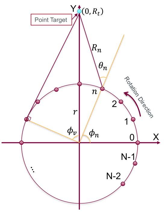
Consider a stationary ROSAR system in Fig. 1. The radar is moving along the edge of a circle centered at the origin with radius . The bore-sight of the antenna always faces outwards along the radial directions. The antenna radiation pattern in azimuth is assumed to be cosine-shape and non-zero within . The radar transmits chirp signals at a constant rate, e.g., times per circle. Due to the symmetry, without loss of generality, we define a 2D coordinate frame such that a point target distance away from the circle center locates at and the first (indexed by 0) phase center (with respect to the -axis counter-clock wise) is at . Then, the bore-sight direction of the antenna at the -th radar position (phase center) is
| (1) |
where . Let and be the distance and the direction from the -th phase center to the target with respect to its bore-sight direction, respectively. Due to the cosine antenna beam pattern, the target is in the field of view (FoV) of only a subset of antenna positions. Denote by the angle such that if , the target is visible to the -th phase center. , and can be derived from trigonometry relationships, i.e.,
| (2) | |||||
| (3) | |||||
| (4) |
The indices of the phase centers where the target is in their FOV are given by
| (5) |
where , and . To generate the image of the target, only signals received by those phase centers are used.
II-B Signal Model and Preprocessing
Let the chirp signal transmitted by the radar be
| (6) |
where is the carrier frequency, is the chirp slope and is the fast time. The received signal at the -th phase center is
| (7) |
where combines the complex reflection coefficient of the target, the antenna radiation pattern and channel fading, is the round-trip time delay, is the speed of the light, is the Gaussian white noise at the receiver side. Specifically, the antenna radiation pattern is represented as
| (8) |
After down-converting and deramping, the resulting intermediate frequency (IF) signal is
| (9) |
where . The residual video phase (RVP) term is negligible compared with other phase terms. Let the sampling frequency, the total number of samples, sampling interval, sampling start time in one chirp be , , (), , respectively. The sampled IF signal is
| (10) |
where is the sampling index, . Combining all the samples, we get the following vector representation
| (11) |
where . Let . Substituting the ’s in each entry by and rearranging items in (11), we have
| (12) |
Now, the data matrix from the effective phase centers used for SAR is
| (13) |
The conventional BPA images a point with parameter by computing the Hadamard product of and a matrix of size , where the element locating at the -th row and -th column is
Then, the intensity of the point is
| (14) |
where is the symbol of Hadamard product. If the target indeed locates at in polar coordinates, all the phases of the sampled data are perfectly compensated, and (14) achieves its maximum. However, the computation complexity of imaging a rectangular area using conventional BPA is , where and is the number of grids along and direction of the area. Clearly, the complexity grows linearly with , and area size. From the complexity analysis, it can be deduced that two possible ways to lower the complexity of BPA are, (1) reducing the number of phase centers to be used, i.e., reducing , and (2) apply range-dimension matched filtering and select the appropriate range bin instead of using all data samples in each pulse.
In the subsequent sections, we first develop a Sparse Array Synthesis (SAS) method that selects a subset of the phase centers and assigns appropriate complex weights. Then, we investigate the use of range-dimension matched filter (or more commonly known as range FFT) to further reduce computation complexity. The two approached are abbreviated to “SAS” and “FFT+SAS” respectively for simplicity.
II-C Problem Formulation for Robust Sparse Array Synthesis
For simplicity, we assume that the reflection coefficient is always 1. Due to complex multipath reflection, wall penetration in indoor environments and the small diameter of the rotation platform relative to the dimension of the environment, the channel fading factor can be approximated to be a constant for the same range bin in all directions and thus we omit it in the formulation. Thus,
| (15) |
BPA can be viewed as a form of range-azimuth two-dimension filtering. To generalize it to sparsely-selected phase centers, we first apply a compensation matrix to to remove the phase items related to fast-time sampling, i.e.,
where the -th row and -th column element of is . The steering vector of the ROSAR array to a near-field target located at range can be represented as
| (16) |
where , and the array pattern can also be calculated as
| (17) |
where is a sparse complex weight vector to be designed and some of its elements can be equal or be close to zero. Note that, is also a function of , but we omit the subscript for simplicity. To focus a point target locating at , we need to compute
where is the Khatri-Rao product.
Due to the vibration of the rotation platform, odometry errors and antenna pattern mismatch (e.g., cosine pattern), there exist array manifold errors, which may lead to blurred images. To obtain an SAR image with good quality in this situation, the sparse weight vector must be carefully designed with consideration of robustness to array errors.
We formulate the way to obtain the desirable as to solve an optimization problem. In the optimization, the first constraint is that the power of the main-lobe peak, locating at , should be larger than or equal to a threshold , i.e.,
| (18) |
where is the array error vector caused by measurement and imperfect radar rotations, and we assume that is bounded by a ball with radius (). Second, to restrict the main-lobe width and the sidelobe level, we put limitations on the received power at some uniformly spaced discrete directions except for the desired main lobe area, i.e.,
| (19) |
where is the error vector for sidelobe area with the same properties as , is the number of uniformly spaced discrete directions, , is the half of the desirable main-lobe width, is the pre-set power ratio of the main-lobe to the sidelobe. Third, to avoid amplifying the noise level, we impose a constraint on the gain of noise power:
| (20) |
Lastly, to guarantee a sufficient gain on the target, we set another constraint .
The objective is to minimize the number of virtual phase centers given by . To this end, we formulate the sparse array synthesis problem as
| (21) |
Problem (21) is a non-convex optimization problem since both the objective function and constraints C1 and C3 are non-convex. Because of the consideration of robustness to array errors, the problem formulation is markedly different from those in conventional sparse array synthesis[23, 24, 25, 26, 27, 28], rendering existing techniques inapplicable. In the next section, we develop a customized algorithm based on FPP and SCA to solve (21).
III Solution Approach for Robust Sparse Array Synthesis (SAS)
III-A Problem Transformation
Directly solving (21) is hard, since -norm minimization problem requires intractable combinatorial search. To reduce the complexity, we replace the -norm objective function with -norm, i.e., as suggested by [29, 30].
C1 and C2 contain additional control variables and to express robustness constraints. They can be simplified by considering the worst case scenarios. Specifically, by using the Cauchy-Schwarz inequality and the triangle inequality, we can find the minimum of main-lobe response and the maximum of sidelobe response respectively as follows
| (26) |
| (31) |
The equalities hold when (). Substituting (26) and (31) into C1 and C2, we obtain the worst-case constraints as
| (32) | |||||
| (33) |
Taking the square root of both sides of (32) and (33), and re-arranging items in the inequalities, we have
| (34) |
| (35) |
where . in (21) can be replaced by two inequality constraints as
| (36) |
| (37) |
and is replaced by
| (38) |
where . The optimization problem is thus transformed to
| (39) |
III-B FPP-SCA-based Algorithm
The reformulated problem (39) is still non-convex which is hard to be solved directly, and it is also tricky to find feasible initial solutions, but it is now amenable to the convex approximation technique. Inspired by the idea of FPP [21], we introduce three slack variables , , () for C1–C4, and we construct the following slacked surrogate problem of (39)
| (40) |
where () is a pre-set coefficient to penalize constraint violations.
To handle the non-convex terms in above constraints, i.e., in , in and in , we next apply SCA [22]. SCA is an iterative method and its core idea is to replace non-convex terms with convex approximations (usually upper bounds of these non-convex terms) in each iteration. In our case, given after the -th iteration, the convex upper bounds of the three non-convex terms are derived by applying their respective first-order Taylor expansions as
| (41) |
| (42) |
| (45) |
Replacing the non-convex terms in C1, C2 and C4 with the convex upper bounds in (41)–(45), we finally transform (21) to a convex sub-problem in (46). {strip}
| (46) |
Repeatedly solving (46) with the values from the previous iteration until the number of iterations reaches a pre-set value . Let be the value of the objective function after the -th iteration, be a vector of target range bins of concern, be a vector of the maximum -norm of for all range bins. Algorithm 1 and 2 summarize the proposed approaches to determine the sparse weight vector for each range bin and to apply the resulting weight vector for SAR imaging, respectively.
III-C Initial values and parameter settings for Algorithms 1 and 2
III-C1 Initial Value Settings
The proposed approach is able to work with any initial values of the control variables since the constraints are always feasible due to the introduced slack variables. In our implementation, the initial value of is chosen as and .
III-C2 Parameter Settings
To ensure convergence, and can be set to around and , respectively. and are design parameters of the sparse array. We found that any value lower than both and makes the SCA diverge. should be chosen by considering practical limitations of target platforms. For example, in Section IV-A, the simulation setup and experiments take the unstable rotation speed of a ROSAR platform into account. The direction of each phase center under unstable rotations is modeled as a Gaussian distribution
| (47) |
where the is the standard deviation of the direction. The error vector is computed from , where is determined by substituting with . Let . By repeatedly sampling from (47), we can obtain the cumulative distribution function (CDF) of , and choose the corresponding to 99% of the cumulative probability as . The testbed evaluations in Section IV-F show that this model is reasonable in realistic settings. Note since the phase error differs among range bins, one specific must be pre-computed for each range bin.
To ensure accurate results, the angle interval should be less than or equal to the angular resolution of ROSAR. However, reducing the angle interval increases the number of grid points and leads to higher computation costs. Since there is no closed-form solution to the angular resolution of a circular array, we use the results of a linear array as a reference. The determination of is based on the expected image quality in target applications. It should be large enough to guarantee a sufficient gain for all range bins. Otherwise, there could be light and dark strips on the generated SAR image.
Increasing improves the sparsity of but when is too large, (36) is no longer feasible. As a general rule of thumb, should be several times larger than the maximum of to ensure that the slack variables converge to zero. Since the -norm differs -norm and cannot enforce sparsity in itself, we must manually set any term in lower than a pre-defined threshold to 0. Thus, in Algorithm 2, only the nonzero entries in are included in computing . Moreover, a final step must be taken to verify the solution. This can be accomplished by checking if the slack variables are sufficiently small, i.e., and is set to in the experiments.
III-D Complexity Reduction for Real-implementation
Since applying range compression along fast time samples[31] (denoted as “FFT+BPA”) can reduce the processing time of conventional BPA, we borrow its idea to further reduce the complexity of the proposed SAS approach (denoted as “FFT+SAS”). Ignoring the noise term in (10) and applying range-FFT to , we have
| (48) | |||||
where and is the number of range bins. Let . We have
| (49) |
and reaches the maximum for
| (50) |
which is the range bin where the target is located. The data vector at the -th phase center now becomes
| (51) |
The data matrix from effective phase centers used for SAR is given by
| (52) |
To focus a point locating at in polar coordinates, we need to compute
| (53) |
where and represents the -th entry of the vector . in (53) can be the sparse weight vector of the corresponding range bin determined by Algorithm 2, or the weight vector of BPA with the -th entry being .
Remark 1
The steering vector may differ from the origin one in (16) after applying range-FFT, since substituting (50) into (49) cannot fully cancel the phase summation term in some cases (e.g., when is not multiple of the length of range bin). In our implementation, is still obtained from the original steering vector. Thus, the array pattern could deviate from the desired one. However, doing so can lead to computation reduction.
Remark 2
The computation complexity of SAS is , where is number of phased centers corresponding to non-zero weights. is typically less than a half of . As for FFT+SAS, the computation complexity is given by . When , the second term dominates. Thus, the overall reduction in complexity by combining FFT and SAS is substantial compared with that of the conventional BPA algorithm. Since the proposed algorithms conduct filtering pixel-by-pixel independently, they can be further accelerated by separating these pixels into multiple groups and processing them in a parallel manner.
IV Performance
In this section, we conduct experimental study to evaluate the effectiveness of the proposed ROSAR imaging algorithms.
IV-A Hardware and Software Implementation
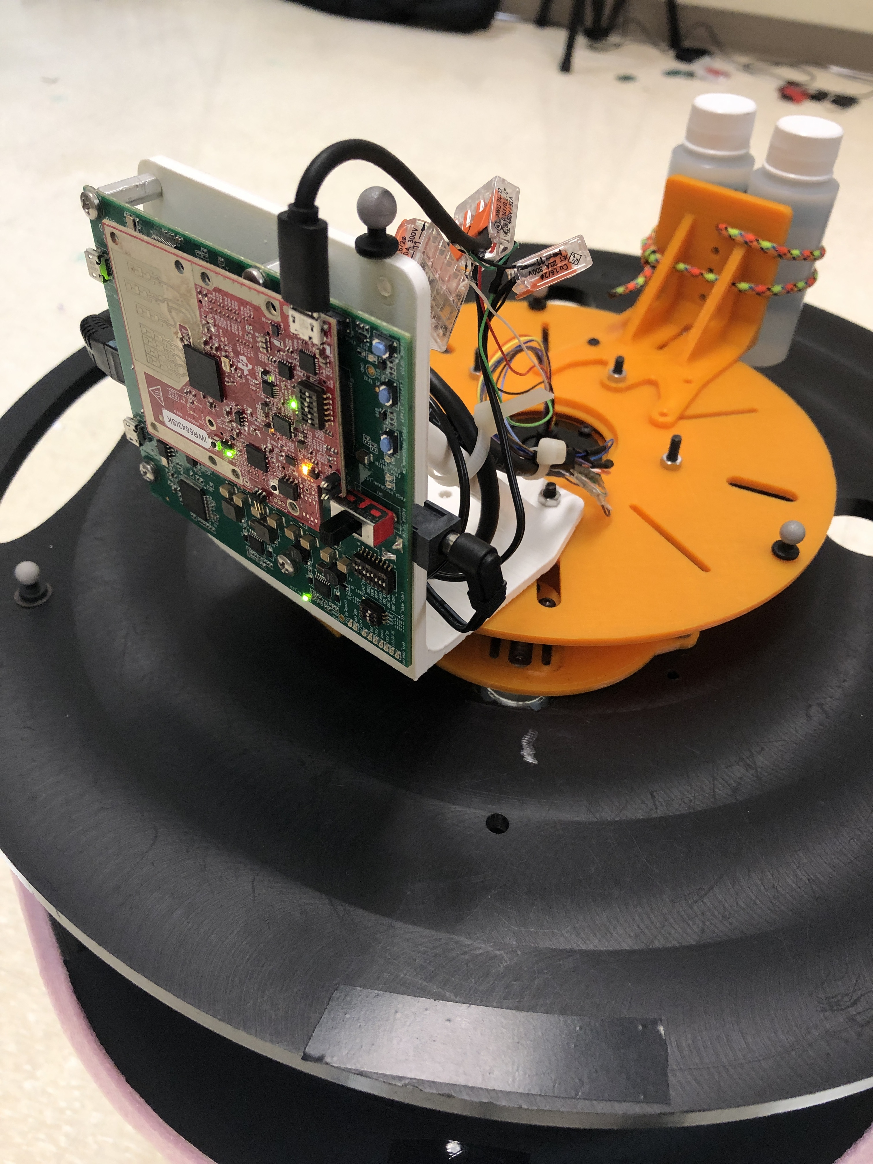
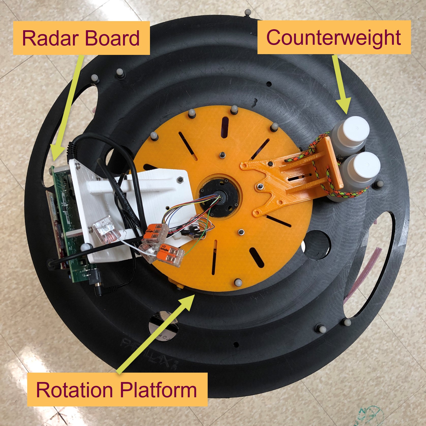
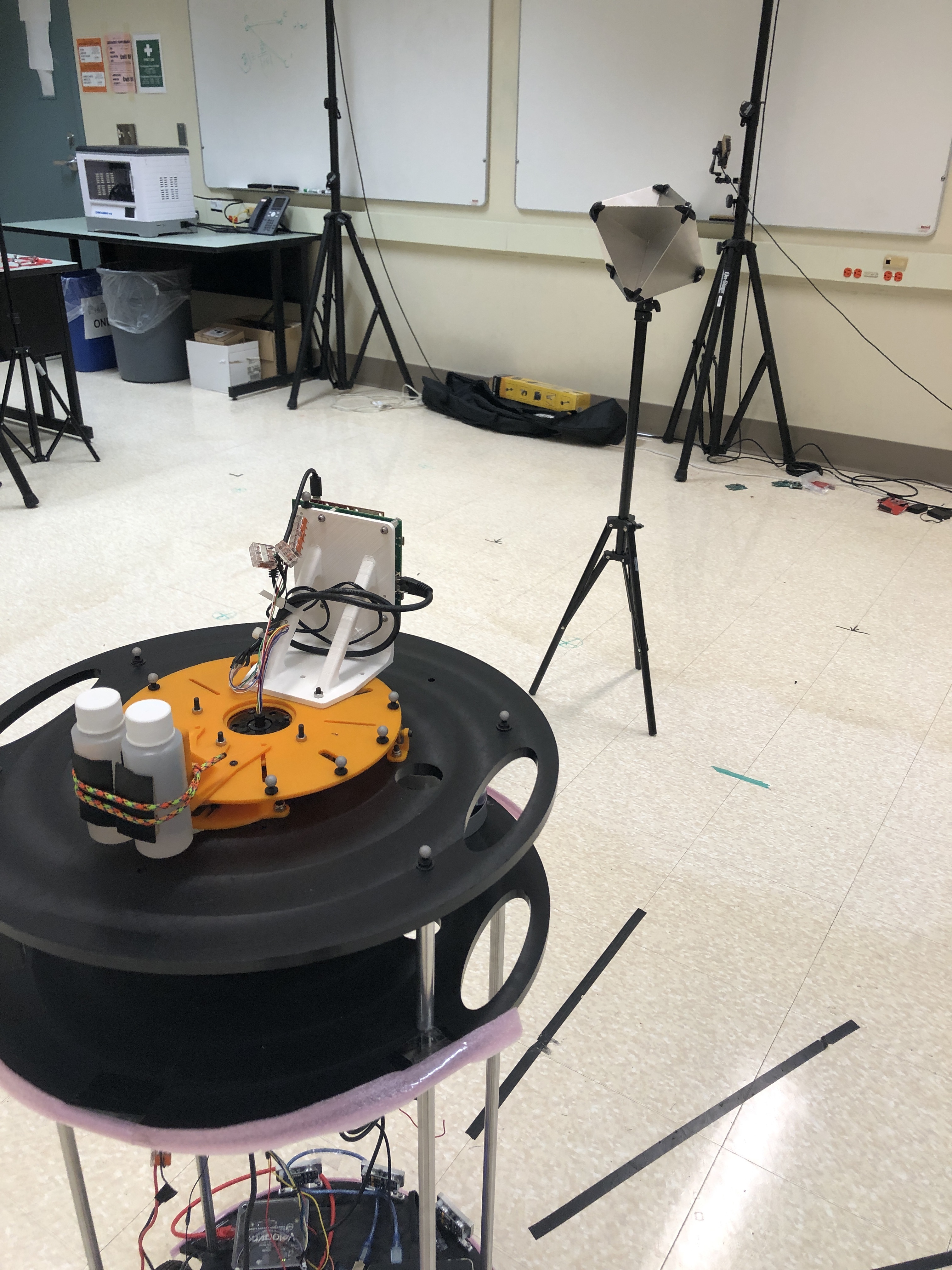
We implement the proposed algorithms on a PC equipped with an Intel Core 8700 CPU and 16GB RAM. The PC has been installed MATLAB and Phased Array Toolbox. We also build a real ROSAR system, which hardware consists of a radar board, a rotation plate, motor and odometry sensors mounted on a rover platform as shown in Fig. 2. The radar uses is Taxes Instruments IWR6843ISK, which generates millimeter wave (mmWave) signals. A 3D-printed plate holding the radar and counter weight is connected to a step motor and a wheel encoder.
The whole system is controlled by Robot Operating System (ROS), including the radar signal sending/receiving and rotation speed. Radar data is collected from the antenna board and angle reading is obtained from the encoder of the rotation platform. Both data is streamed to the PC and processed by MATLAB programs for SAR imaging.
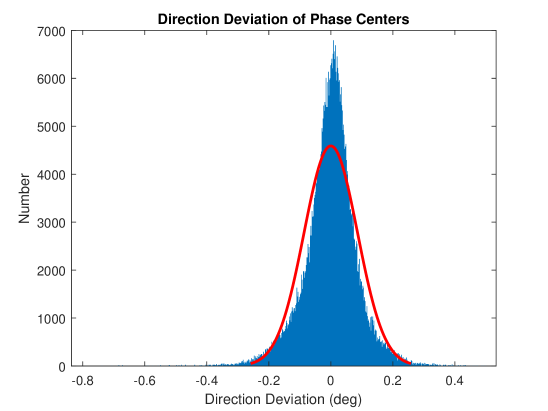
To estimate phase center errors from wheel encoder, we mount several optical markers on the rotation plate. Markers can be tracked by OptiTrack, an optical motion capture system treated as ground truth (position accuracy: 0.2 mm). We rotate the platform multiple rounds and compare the angle difference between the data from tick’s encoder and the OptiTrack system. Fig. 3 shows the mean value is degree. If the data is fitted by a Gaussian distribution, the standard deviation is . Thus, we can assume the direction of the -th phase center follows .
IV-B Parameter Settings
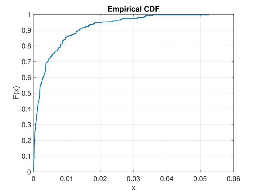
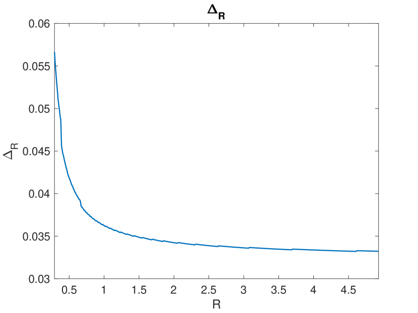
The detailed parameters of the ROSAR system are summarized in Table II. From the settings, the range resolution is given by , where is the bandwidth of the sampled chirp signal. The maximum unambiguous range is . If we choose to represent 99% of the probability of the cumulative distribution function (CDF), Fig. 4(a) shows an example CDF for and . Fig. 4(b) shows as a function of range, from which we can see decreases as the range becomes larger. It is because a small displacement from the desirable positions of phase centers has less impact when the radar is further away from the target. The detailed calculation steps have been given in Section III-C2.
| Radar Settings | |
|---|---|
| 0.145 m | |
| Rotation speed | 60 RPM |
| Rotation time | 1 s |
| # Of TX | 1 |
| # Of RX | 1 |
| Antenna Pattern | Cosine |
| Antenna FOV | [-90°, 90°] |
| Start rotating direction | 0° |
| Rotation direction | Counter-clockwise |
| TX power | 12 dBm |
| Antenna gain | 7 dBi |
| RX gain | 48 dB |
| Chirp Signal Settings | |
| Start Frequency | 60 GHz |
| End Frequency | 64 GHz |
| Ramp start time | 0 us |
| Ramp end time | 58 us |
| 7 us | |
| Sampling end time | 57 us |
| 4.5 MHz | |
| 225 | |
| 800 | |
| Hz/s | |
| 225 | |
All the sparse weight vector for each range bin are computed in advance using Algorithm 1 with parameters listed in Table III. We use CVX and Mosek solver[32] to find the optimal values in each iteration of SCA.
| 50 | |
| 0.001 | |
| 1° | |
| Sampled angle interval | 0.5° |
| 50 | |
| 0.0005 (-33 dB) | |
| 5 |
IV-C Baseline Algorithm and Metrics
We implement four algorithms: “BPA”, “FFT+BPA”, “SAS”, “FFT+SAS”, “RBPA” (BPA with randomly selected phase centers) and “FFT+RBPA” for different comparison purposes. The following metrics are used in quantitative evaluations:
-
•
Half main lobe width : The half main lobe width is defined as the angle interval between the peak and the closest local minima on either side of the main lobe.
-
•
Peak-to-integral sidelobe ratio (PISR): The PISR for a specific range bin is calculated as
| (54) |
-
•
SAR computation cost: The elapsed time of generating a SAR image.
-
•
Image entropy [33]: Let be the total energy of the image, and be the energy density of a pixel. The image entropy is defined as
| (55) |
The targets are well focused on the SAR image if is large and is small.
IV-D Numerical Results and Analysis
IV-D1 Solution to the Optimization Problem
We first give the numerical result through imaging a point target locating at . In this case, the number of effective phase centers, i.e., the length of synthesized aperture, is calculated to be 381 by (5). Fig. 5 shows the magnitude of each element in out and robust design, respectively. In both cases, we can see is less than a half of the total number of phase centers from Table IV. However, the robust design, the sparsity is slightly reduced.
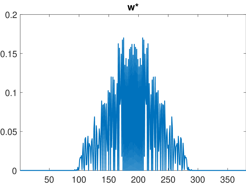
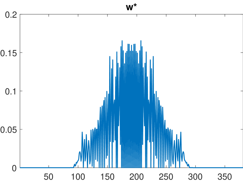
| Non-Robust () | 141 | 8.21 |
| Robust () | 157 | 8.38 |
IV-D2 Array Pattern
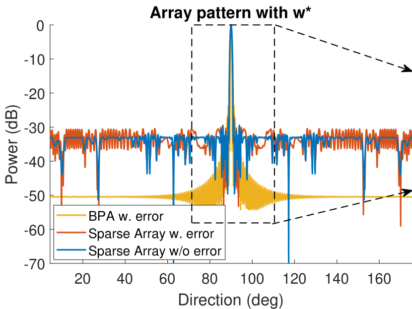
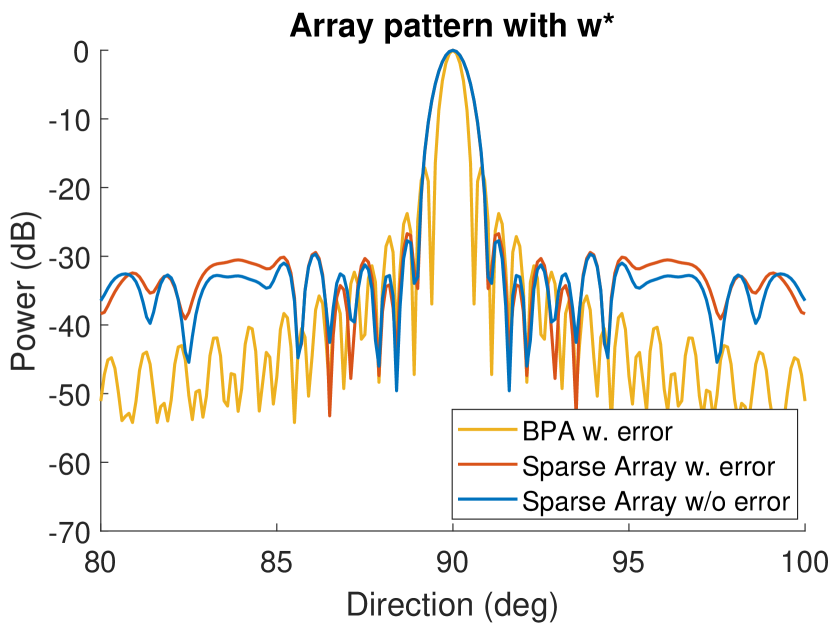
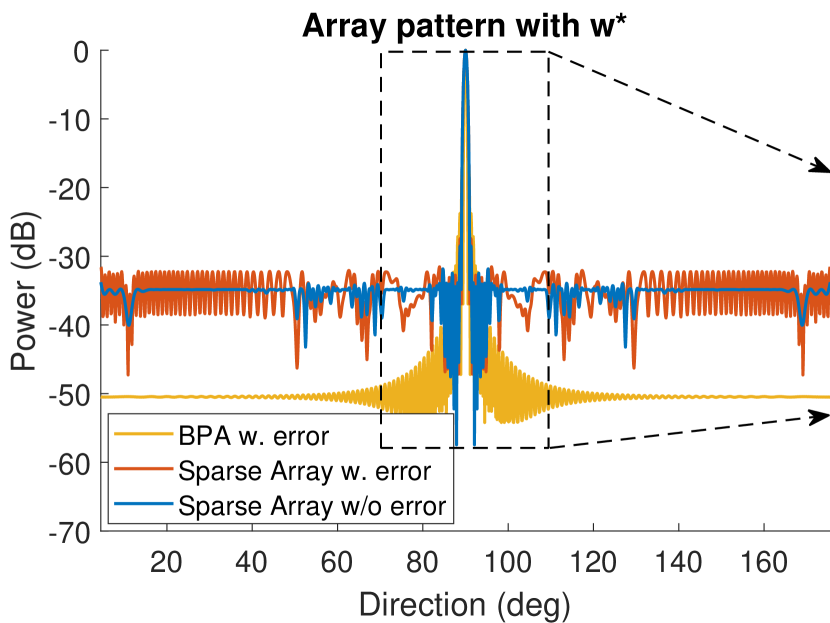
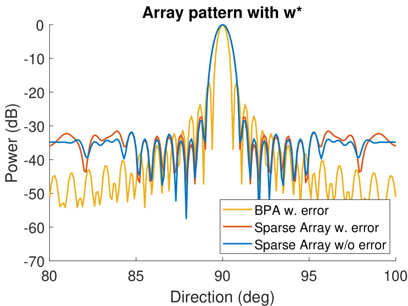
Fig. 6 shows the array patterns of the SAS out and considering robust design for . Fig. 6(b) and Fig. 6(d) are the main lobe area of Fig. 6(a) and 6(c). The array pattern is calculated by for . The blue and red lines show the array pattern out and adding phase errors , respectively. The yellow line is the array pattern of BPA phase errors. As we can see, the main lobe is in , which meets the design parameters. As shown in Fig. 6(a), the power of the sidelobes when there is no error in the steering vector is mostly -33dB lower than that of the main lobe peak. The few exceptions fall in between angle grid points of interval 0.5° and thus their power levels are not enforced by the constraints. Although denser grid points (and consequently more constraints) can reduce the chance of requirement violation, the computation cost of SCA grows drastically. When there are errors in the steering vector, most of the sidelobes do not meet the -33dB criteria in non-robust design. In contrast, the robust design (the red line in Fig. 6(c)), this is no longer the case. Furthermore, the average power of the sidelobes is lower than -33dB robust design even in absence of steering vector errors. This is due to the worst case assumption of robustness design as evident in (34) and (35). The PISRs are given in Table V. High values are better. The conventional BPA gives the best PISR due to its low sidelobes but needs much more computation time.
| Algorithms & Settings | w/o error | w. error |
|---|---|---|
| SAS w. Robust | 0.1256 | 0.1253 |
| SAS w/o robust | 0.1308 | 0.1303 |
| BPA w. error | N/A | 0.2339 |
IV-D3 Results for All Range Bins
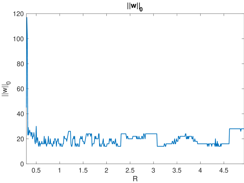
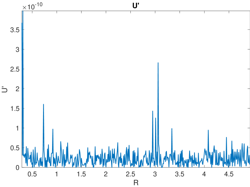
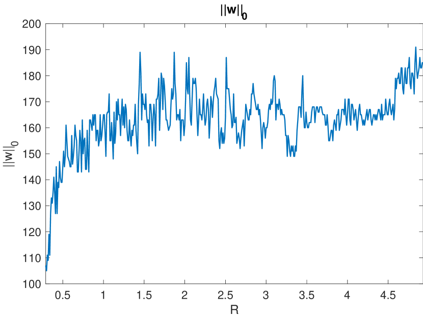
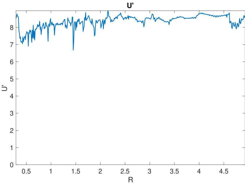
Fig. 7 shows the values of and for all range bins when . Clearly, the sparsity of the array holds in all range bins. We observe that all s are small. In this case, although the array is very sparse, the SNR is low (recall that is the magnitude of main-lobe peak and the noise power is constant from C3). Setting can bound the SNR at the cost of reduced sparsity as shown in Fig. 8.
IV-E SAR Imaging Simulation for a Point Target
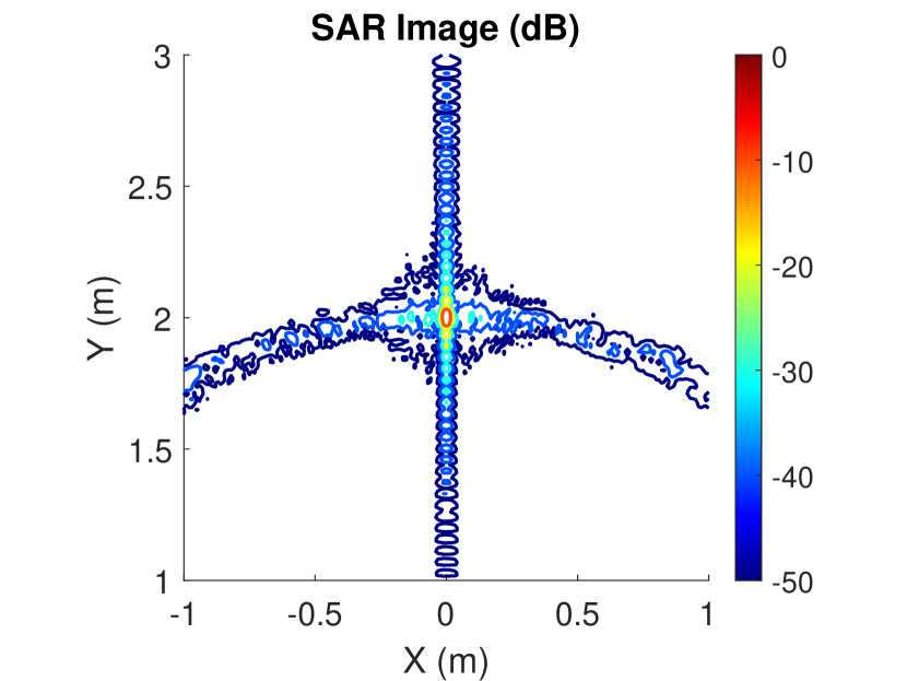
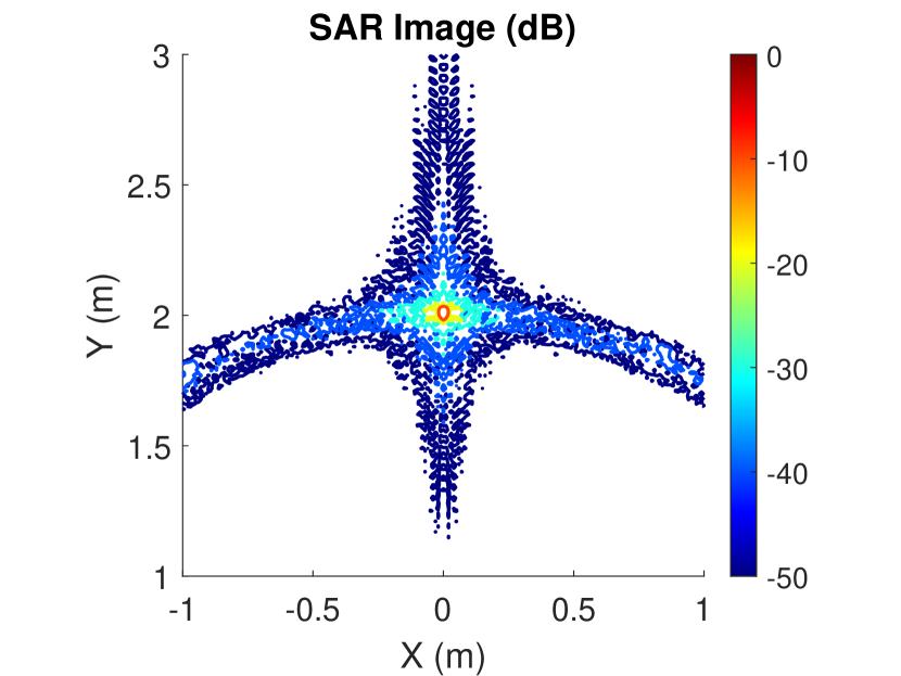
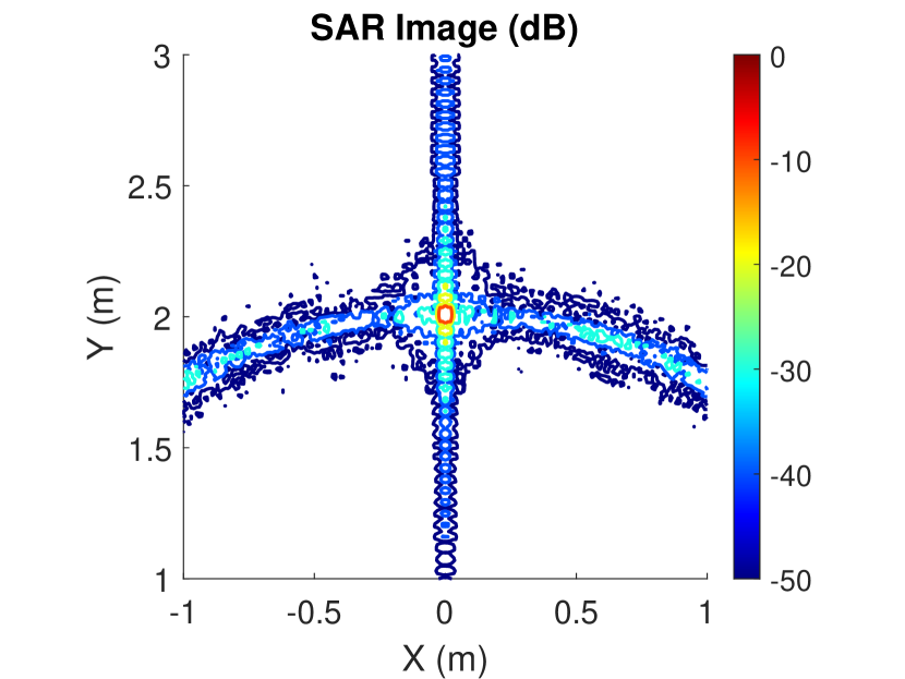
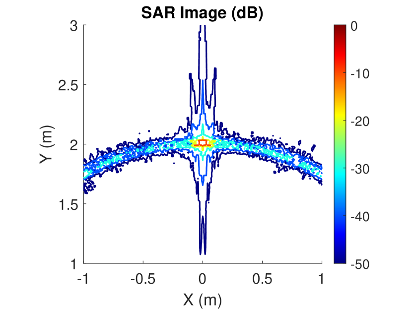
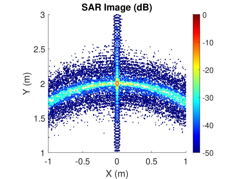
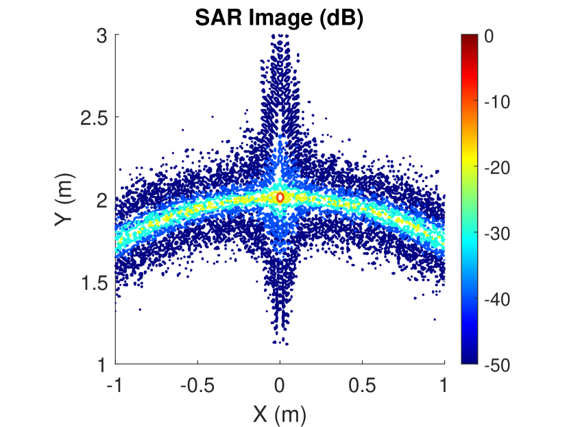
By using MATLAB Phased Array Toolbox, we simulated a point target locating at , a rotating radar and the sending/receiving signals of radar antennas. Fig. 9(a), 9(c) and 9(e) show the imaging results of the target area by conventional BPA, SAS and RBPA, while Fig. 9(b), 9(d) and 9(f) show the SAR images by employing FFT acceleration. The SAR image quality and computation cost is summarized in Table VI. Although the entropy of the SAR image generated by SAS is slightly worse than that by BPA, the computational time is significantly reduced. Furthermore, although BPA with randomly selected phase centers takes less time as well, the resulting image quality is much worse than others.
| Algorithm | Time Cost (s) | |
|---|---|---|
| BPA | 3.7489 | 43.66 |
| FFT + BPA | 3.9812 | 29.43 |
| SAS | 4.4073 | 18.03 |
| FFT + SAS | 4.4703 | 3.61 |
| RBPA | 5.7850 | 18.03 |
| FFT + RBPA | 5.8728 | 5.86 |
IV-F Testbed Evaluation
Although simulations can provide insights on the impacts of configuration parameters and the performance of the proposed approach in simulated environments, existing packages in MATLAB cannot model the reflection, diffusion and deflection properties of mmWave signals in indoor environments well. In this section, the performance and efficiency of the proposed approach is validated through two real-world experiments. The size of SAR area is set to be 9.8756m9.8756m with grid size being 0.04m0.04m.
IV-F1 Scenario 1: Corner Reflector
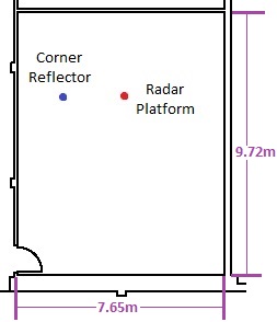
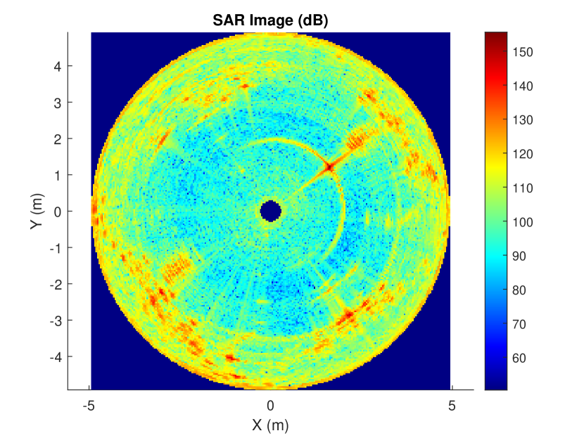
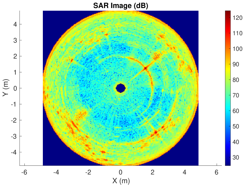
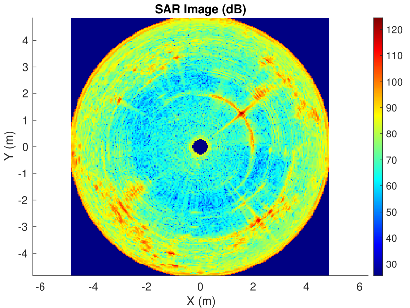
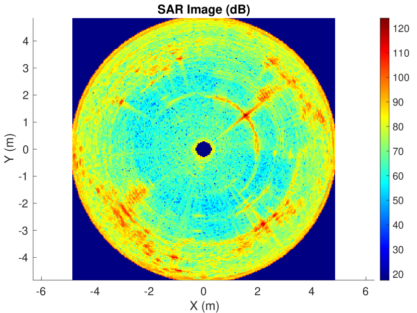
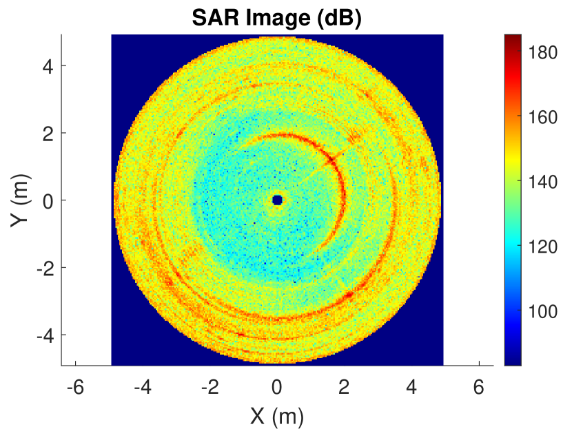
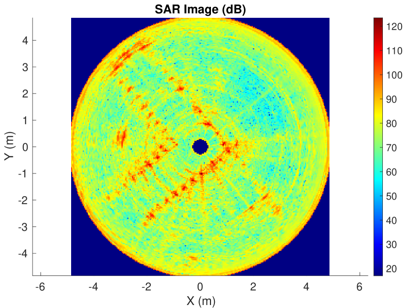
We put a radar platform (red dot) and a corner reflector (blue dot) in a lab (see Fig. 10). In addition to a corner reflector which can be treated as the point target with strong reflection in practice, there are also computer desks, wood cabinet, metal cases and other equipment in the environment. Fig. 11, 12 and 13 illustrate the SAR images under different algorithms and settings. The numerical results are summarized in Table VII. It can be observed from the figures, BPA gives the clearest image among all approaches. The inclusion of robust design can improve sharpness of the image. At and dB, the image entropy from SAS is comparable to that of the BPA but takes only one fifth of the total computation time. Range-FFT can work in conjunction with both BPA and SAS. When comparing all these figures, we find that range-dimension match filtering degrades image sharpness slightly. This is also corroborated by the image entropy results in Table VII. Among all approaches, “FFT+SAS” incurs the least amount of compute time – close to 13 times faster than BPA while achieving acceptable image quality.
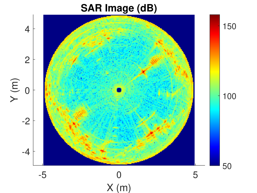
algorithm
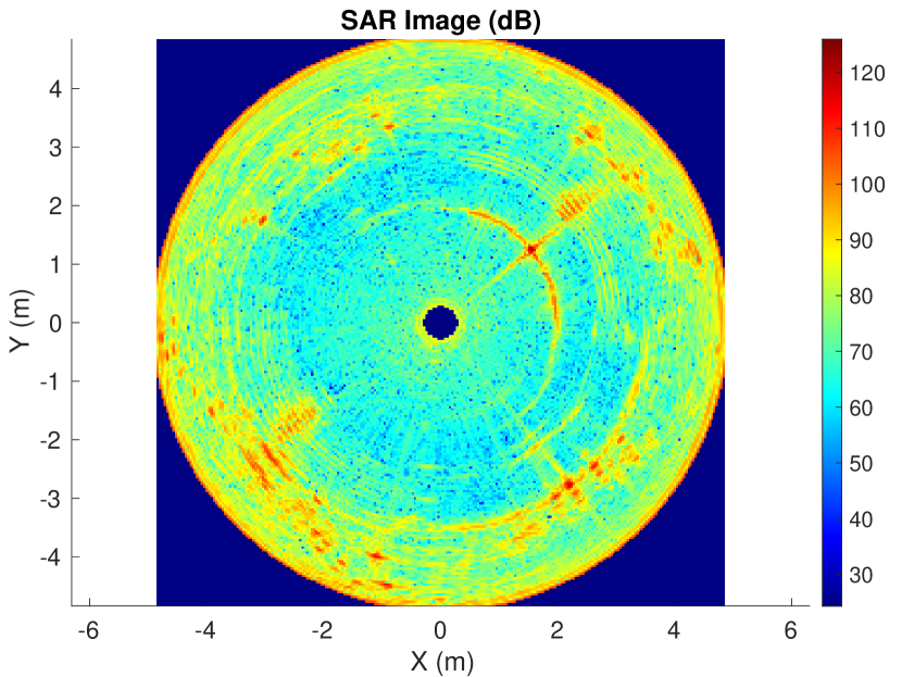
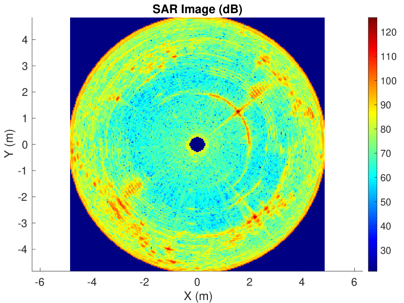
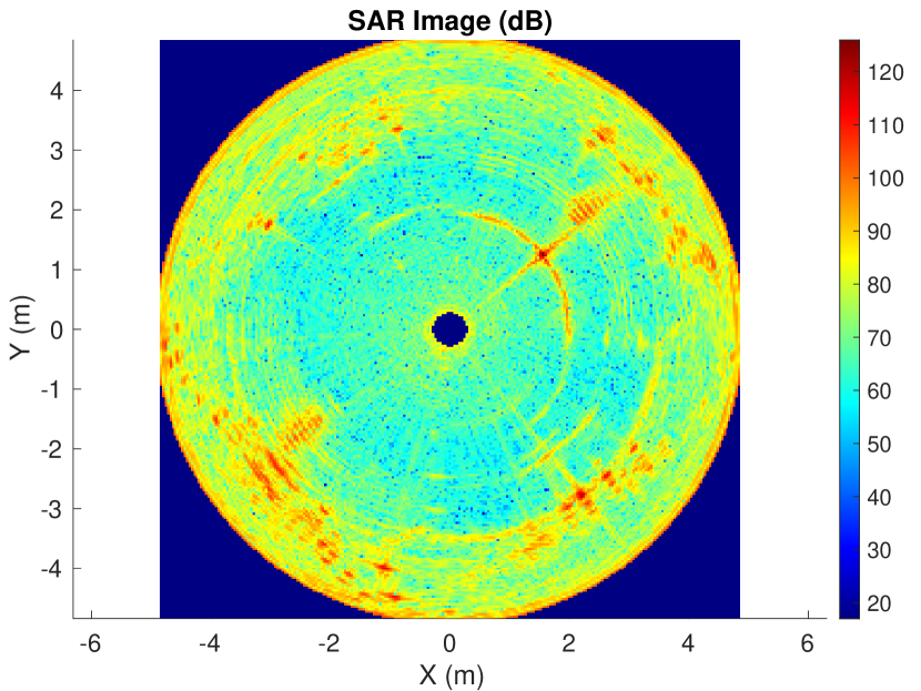
algorithm

| Algorithm | Settings | Time Cost (s) | |
|---|---|---|---|
| BPA | N/A | 6.0472 | 151.84 |
| FFT+BPA | N/A | 6.3400 | 21.69 |
| SAS | ,dB,w/o Robust | 7.2607 | 28.04 |
| ,dB,Robust | 7.1717 | 28.94 | |
| ,dB,Robust | 6.8913 | 30.56 | |
| FFT+SAS | ,dB,w/o Robust | 7.3989 | 11.45 |
| ,dB,Robust | 7.3227 | 12.14 | |
| ,dB,Robust | 7.1170 | 12.31 | |
| RBPA | N/A | 8.3060 | 25.02 |
| FFT+RBPA | N/A | 8.3179 | 13.07 |
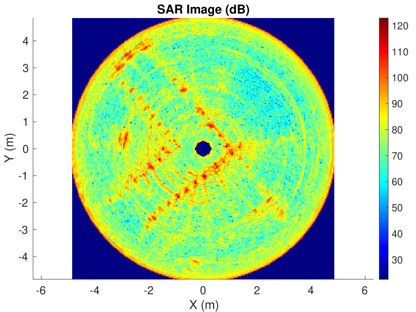
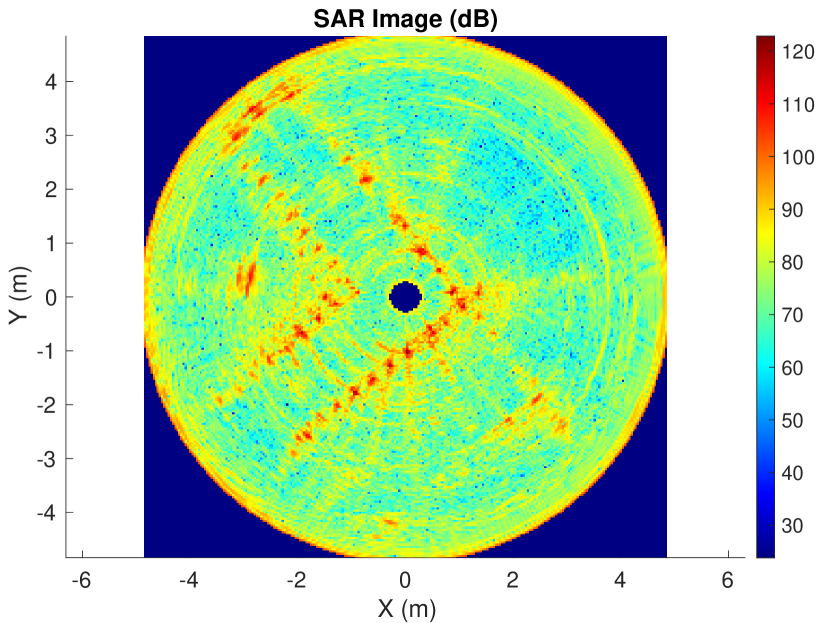
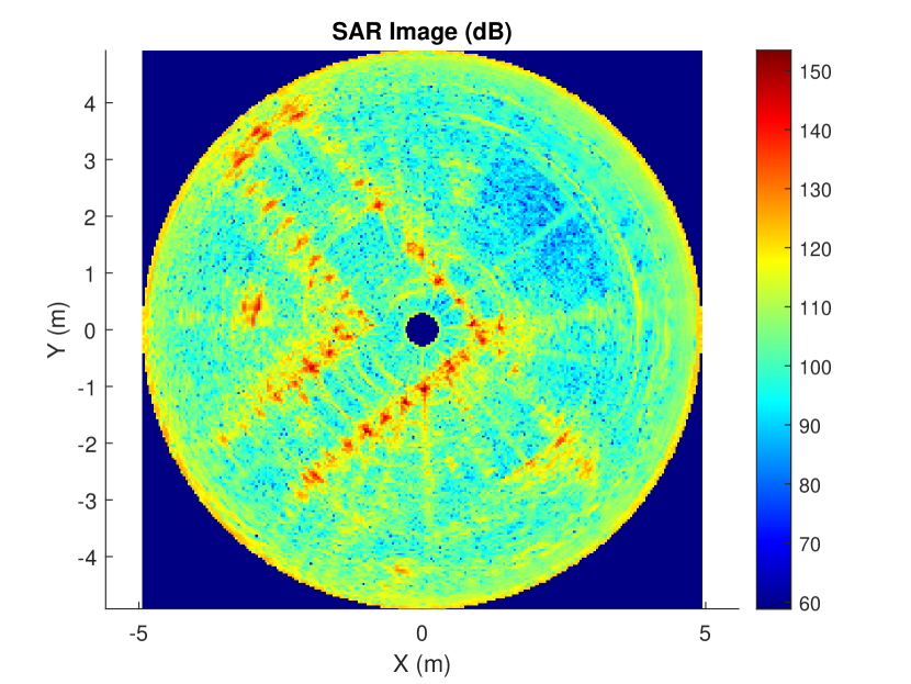
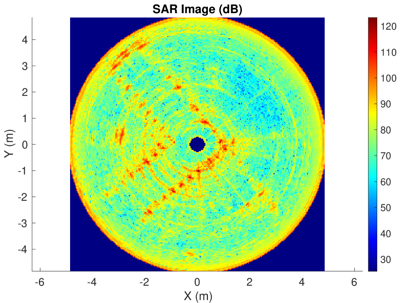
IV-F2 Scenario 2: Corridor Corner
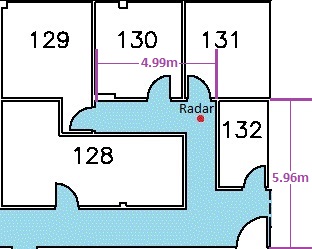
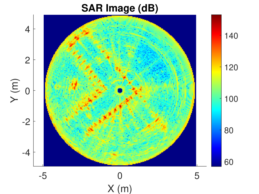
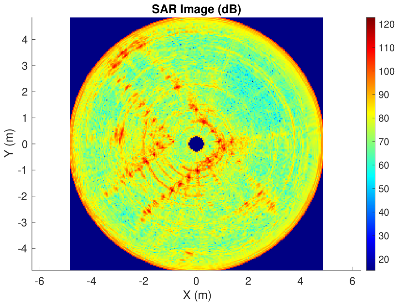
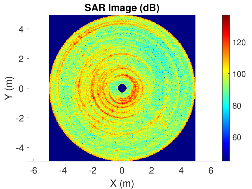
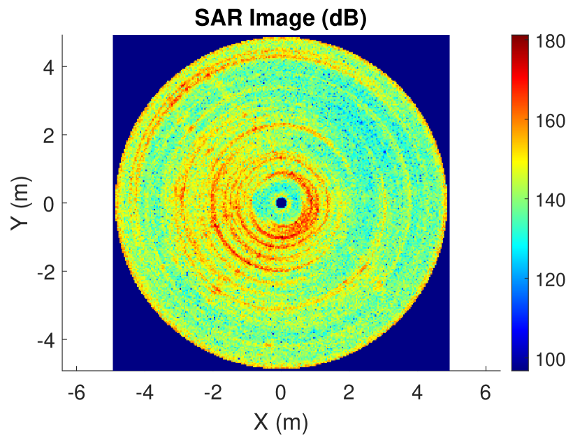
Next we collect data from the corner of a corridor. The floor map is given in Fig. 14, where the red dot indicates the location of the system, the blue area corresponds to the corridor and the white space with labels represents different rooms. Figs. 15, 16 and 17 show the SAR images from different algorithms and parameter settings. The numerical results are summarized in Table VIII. From the figures, one can discern the outline of the corridor corner. Due to the penetration of mmWave signals through drywalls, the steel bars inside the walls are visible in the figures. Additionally, an object in the Room 128 and the contour of Room 132 are also visible. Similar to the case with corner reflector, the consideration of robust design can indeed improve image quality. When is set to -33dB and robust design, the sidelobes are less visible. Moreover, inclusion of range-domain FFT can indeed greatly reduce the compute time. BPA with randomly selected phase centers takes less time, but the generated image is blurred. The proposed robust design, with and dB, gives comparable image quality as that of BPA and consume much less computation time.
algorithm
algorithm

| Algorithm | Settings | Time Cost (s) | |
|---|---|---|---|
| BPA | N/A | 6.4436 | 151.22 |
| FFT+BPA | N/A | 6.6881 | 21.85 |
| SAS | ,dB,w/o Robust | 7.3802 | 27.75 |
| ,dB,Robust | 7.2871 | 29.30 | |
| ,dB,Robust | 7.0251 | 30.25 | |
| FFT+SAS | ,dB,w/o Robust | 7.5309 | 12.50 |
| ,dB,Robust | 7.4562 | 12.21 | |
| ,dB,Robust | 7.2425 | 12.47 | |
| RBPA | N/A | 8.3671 | 25.35 |
| FFT+RBPA | N/A | 8.3801 | 13.28 |
V Conclusion
In this paper, we propose a new fast imaging algorithm based on robust sparse array synthesis for ROSAR. Since radar path is circular, such an algorithm only needs to pre-compute the complex weights of the imaging filter offline for one direction per range bin. Due to the external influence could affect the sidelobe level, we add robust design to maintain the image quality. To meet our pre-set expectation and solve this problem, our proposed algorithm employs feasible point pursuit and successive convex approximation technology. On that basis, we also give another algorithm based on range-FFT to further reduce the computation complexity.
According to the simulation and testbed results, we conclude that our approach can generate an SAR image with the quality comparable to that of BPA. Meanwhile, the proposed approach is able to reduce the computational cost significantly and is robust to the array error.
Nonetheless, we must sacrifice some image quality if employing FFT-based range-dimensional matched filtering. Thus, exploring a better approach for the processing based on range FFT is our future research direction.
References
- [1] C. Willey, “Synthetic aperture radars–a paradigm for technology evolution,” IEEE Trans. Aerospace Elec. Sys, vol. 21, pp. 440–443, 1985.
- [2] A. Moreira, J. Mittermayer, and R. Scheiber, “Extended chirp scaling algorithm for air-and spaceborne sar data processing in stripmap and scansar imaging modes,” IEEE Transactions on geoscience and remote sensing, vol. 34, no. 5, pp. 1123–1136, 1996.
- [3] H. Klausing, “Feasibility of a synthetic aperture radar with rotating antennas (rosar),” in 1989 19th European Microwave Conference. IEEE, 1989, pp. 287–299.
- [4] F. Ali, A. Urban, and M. Vossiek, “A short range synthetic aperture imaging radar with rotating antenna,” International Journal of Electronics and Telecommunications, vol. 57, pp. 97–102, 2011.
- [5] D. Li, H. Liu, Y. Liao, and X. Gui, “A novel helicopter-borne rotating sar imaging model and algorithm based on inverse chirp-z transform using frequency-modulated continuous wave,” IEEE Geoscience and Remote Sensing Letters, vol. 12, no. 8, pp. 1625–1629, 2015.
- [6] Y. Nan, X. Huang, and Y. J. Guo, “A panoramic synthetic aperture radar,” IEEE Transactions on Geoscience and Remote Sensing, vol. 60, pp. 1–13, 2022.
- [7] J. Zhang, G. Liao, S. Zhu, J. Xu, and F. Liu, “Wavenumber-domain autofocus algorithm for helicopter-borne rotating synthetic aperture radar,” IET Signal Processing, vol. 12, no. 3, pp. 294–300, 2018.
- [8] F. Ali, G. Bauer, and M. Vossiek, “A rotating synthetic aperture radar imaging concept for robot navigation,” IEEE transactions on microwave theory and techniques, vol. 62, no. 7, pp. 1545–1553, 2014.
- [9] I. Cumming and J. Bennett, “Digital processing of seasat sar data,” in ICASSP’79. IEEE International Conference on Acoustics, Speech, and Signal Processing, vol. 4. IEEE, 1979, pp. 710–718.
- [10] D. Zeng, T. Zeng, C. Hu, and T. Long, “Back-projection algorithm characteristic analysis in forward-looking bistatic sar,” in 2006 CIE International Conference on Radar. IEEE, 2006, pp. 1–4.
- [11] M. E. Yanik and M. Torlak, “Near-field mimo-sar millimeter-wave imaging with sparsely sampled aperture data,” Ieee Access, vol. 7, pp. 31 801–31 819, 2019.
- [12] R. K. Raney, H. Runge, R. Bamler, I. G. Cumming, and F. H. Wong, “Precision sar processing using chirp scaling,” IEEE Transactions on geoscience and remote sensing, vol. 32, no. 4, pp. 786–799, 1994.
- [13] R. Zhu, J. Zhou, G. Jiang, and Q. Fu, “Range migration algorithm for near-field mimo-sar imaging,” IEEE Geoscience and Remote Sensing Letters, vol. 14, no. 12, pp. 2280–2284, 2017.
- [14] L. M. Ulander, H. Hellsten, and G. Stenstrom, “Synthetic-aperture radar processing using fast factorized back-projection,” IEEE Transactions on Aerospace and electronic systems, vol. 39, no. 3, pp. 760–776, 2003.
- [15] L. Zhang, H.-l. Li, Z.-j. Qiao, and Z.-w. Xu, “A fast bp algorithm with wavenumber spectrum fusion for high-resolution spotlight sar imaging,” IEEE Geoscience and Remote Sensing Letters, vol. 11, no. 9, pp. 1460–1464, 2014.
- [16] Q. Dong, G.-C. Sun, Z. Yang, L. Guo, and M. Xing, “Cartesian factorized backprojection algorithm for high-resolution spotlight sar imaging,” IEEE Sensors Journal, vol. 18, no. 3, pp. 1160–1168, 2017.
- [17] Y. Luo, F. Zhao, N. Li, and H. Zhang, “A modified cartesian factorized back-projection algorithm for highly squint spotlight synthetic aperture radar imaging,” IEEE Geoscience and Remote Sensing Letters, vol. 16, no. 6, pp. 902–906, 2018.
- [18] H. Bi, G. Bi, B. Zhang, W. Hong, and Y. Wu, “From theory to application: Real-time sparse sar imaging,” IEEE Transactions on Geoscience and Remote Sensing, vol. 58, no. 4, pp. 2928–2936, 2019.
- [19] B. Zhang, W. Hong, and Y. Wu, “Sparse microwave imaging: Principles and applications,” Science China Information Sciences, vol. 55, no. 8, pp. 1722–1754, 2012.
- [20] C. Wen, Y. Huang, J. Peng, G. Zheng, W. Liu, and J.-K. Zhang, “Reconfigurable sparse array synthesis with phase-only control via consensus-admm-based sparse optimization,” IEEE Transactions on Vehicular Technology, vol. 70, no. 7, pp. 6647–6661, 2021.
- [21] O. Mehanna, K. Huang, B. Gopalakrishnan, A. Konar, and N. D. Sidiropoulos, “Feasible point pursuit and successive approximation of non-convex qcqps,” IEEE Signal Processing Letters, vol. 22, no. 7, pp. 804–808, 2014.
- [22] A. Beck, A. Ben-Tal, and L. Tetruashvili, “A sequential parametric convex approximation method with applications to nonconvex truss topology design problems,” Journal of Global Optimization, vol. 47, no. 1, pp. 29–51, 2010.
- [23] S. E. Nai, W. Ser, Z. L. Yu, and H. Chen, “Beampattern synthesis for linear and planar arrays with antenna selection by convex optimization,” IEEE Transactions on Antennas and Propagation, vol. 58, no. 12, pp. 3923–3930, 2010.
- [24] B. Fuchs, “Synthesis of sparse arrays with focused or shaped beampattern via sequential convex optimizations,” IEEE Transactions on Antennas and Propagation, vol. 60, no. 7, pp. 3499–3503, 2012.
- [25] Y. Liu, Z. Nie, and Q. H. Liu, “Reducing the number of elements in a linear antenna array by the matrix pencil method,” IEEE Transactions on Antennas and Propagation, vol. 56, no. 9, pp. 2955–2962, 2008.
- [26] Y. Liu, Q. H. Liu, and Z. Nie, “Reducing the number of elements in the synthesis of shaped-beam patterns by the forward-backward matrix pencil method,” IEEE Transactions on Antennas and Propagation, vol. 58, no. 2, pp. 604–608, 2009.
- [27] W. P. Keizer, “Linear array thinning using iterative fft techniques,” IEEE Transactions on Antennas and Propagation, vol. 56, no. 8, pp. 2757–2760, 2008.
- [28] W. P. Du Plessis, “Weighted thinned linear array design with the iterative fft technique,” IEEE transactions on antennas and propagation, vol. 59, no. 9, pp. 3473–3477, 2011.
- [29] E. J. Candes, M. B. Wakin, and S. P. Boyd, “Enhancing sparsity by reweighted l1 minimization,” Journal of Fourier analysis and applications, vol. 14, no. 5, pp. 877–905, 2008.
- [30] D. L. Donoho, “Compressed sensing,” IEEE Transactions on information theory, vol. 52, no. 4, pp. 1289–1306, 2006.
- [31] M. T. Crockett and D. Long, “An introduction to synthetic aperture radar: A high-resolution alternative to optical imaging,” 2013.
- [32] M. Grant and S. Boyd, “CVX: Matlab software for disciplined convex programming, version 2.1,” http://cvxr.com/cvx, Mar. 2014.
- [33] G. Xu, L. Yang, L. Zhang, Y.-C. Li, and M.-D. Xing, “Weighted minimum entropy autofocus algorithm for isar imaging,” Journal of Electronics & Information Technology, vol. 33, no. 8, pp. 1809–1815, 2011.
| Wei Zhao received his B.Eng. degree in Automation from Xidian University, M.A.Sc. degree in Electrical & Computer Engineering from McMaster University. He is a Ph.D. candidate in the Department of Computing and Software in McMaster University since 2017. |
| Cai Wen (M’19) received the B.E. degree from the School of Electronic Engineering, Xidian University, Xi’an, China, in 2009, and the Ph.D. degree from the National Laboratory of Radar Signal Processing, Xidian University, Xi’an, China, in 2014. He was a Research Scientist with the China NORINCO Group from Jan. 2015 to Oct. 2016. From Nov. 2019 to Mar. 2023, he was with the Department of Electrical and Computer Engineering, McMaster University, Hamilton, Canada, as a Post-Doctoral Research Fellow. Since Nov. 2016 he has been with the School of Information Science and Technology, Northwest University, Xi’an, China, where he is currently an Associate Professor. His current research interests include sensor array signal processing, MIMO radar signal processing, integrated sensing and communication, and mathematical optimization. |
| Quan Yuan received the Bachelor of Engineering degree from McMaster University, Canada, in 2022. He is currently working towards the Master of Engineering degree on Computing and Software under the supervision of Dr. Rong Zheng at McMaster University, Canada. |
| Rong Zheng received the B.E. and M.E. degrees in electrical engineering from Tsinghua University, Beijing, China, in 1996 and 1998, respectively, and the Ph.D. degree from the Department of Computer Science, University of Illinois at Urbana–Champaign, Champaign, IL, USA, in 2004. She is currently a Professor with the Department of Computing and Software, McMaster University, Hamilton, ON, Canada. |