Interpretability-Aware Vision Transformer

Abstract

Vision Transformers (ViTs) have become prominent models for solving various vision tasks. However, the interpretability of ViTs has not kept pace with their promising performance. While there has been a surge of interest in developing post hoc solutions to explain ViTs’ outputs, these methods do not generalize to different downstream tasks and various transformer architectures. Furthermore, if ViTs are not properly trained with the given data and do not prioritize the region of interest, the post hoc methods would be less effective. Instead of developing another post hoc approach, we introduce a novel training procedure that inherently enhances model interpretability. Our interpretability-aware ViT (IA-ViT) draws inspiration from a fresh insight: both the class patch and image patches consistently generate predicted distributions and attention maps. IA-ViT is composed of a feature extractor, a predictor, and an interpreter, which are trained jointly with an interpretability-aware training objective. Consequently, the interpreter simulates the behavior of the predictor and provides a faithful explanation through its single-head self-attention mechanism. Our comprehensive experimental results demonstrate the effectiveness of IA-ViT in several image classification tasks, with both qualitative and quantitative evaluations of model performance and interpretability.

Introduction

The Transformer architecture (Vaswani et al. 2017), originally designed for natural language processing (NLP) tasks (Devlin et al. 2018), has recently found application in computer vision (CV) tasks with the emergence of Vision Transformer (ViT) (Dosovitskiy et al. 2020). ViT utilizes the multi-head self-attention (MSA) mechanism as its foundation, enabling it to proficiently capture long-range dependencies among pixels or patches within images. As a result, ViTs have demonstrated superior performance over state-of-the-art convolutional neural networks (CNNs) in numerous computer vision (CV) tasks, including but not limited to image classification (Liu et al. 2021a, b; Touvron et al. 2021a; Yuan et al. 2021a; Xu, Cai, and Li 2022), object detection (Carion et al. 2020; Chu et al. 2021; Wang et al. 2022, 2021), action recognition (Liu et al. 2022; Zhang et al. 2021), and medical imaging segmentation (Li et al. 2022, 2023a).

Since ViTs are extensively employed in high-stakes decision-making fields like healthcare (Stiglic et al. 2020; Li et al. 2023b) and autonomous driving (Kim and Canny 2017), there exists a significant demand for gaining insights into their decision-making process. Nonetheless, ViTs continue to function as black-box models, lacking transparency and explanations for both their training process and predictions. To tackle this challenge, explainable AI (XAI) has arisen as a specialized field within AI, with the goal of ensuring that end users can intuitively understand and trust the models’ outputs by providing explanations for their behavior (Samek et al. 2019; Arrieta et al. 2020).

XAI is a rapidly growing field encompassing numerous research directions. One strand focuses on post hoc explanation techniques, which aim to obtain explanations by approximating a pre-trained model and its predictions (Ribeiro, Singh, and Guestrin 2016; Zhou et al. 2016; Lundberg and Lee 2017; Shrikumar, Greenside, and Kundaje 2017; Sundararajan, Taly, and Yan 2017; Petsiuk, Das, and Saenko 2018; Pan, Li, and Zhu 2021; Qiang et al. 2023; Li et al. 2023d). Although there has been an increasing interest in developing post hoc solutions for Transformers, most of them either rely on the attention weights within the MSA mechanism (Hao et al. 2021; Abnar and Zuidema 2020) or utilize back-propagation gradients to generate explanations (Chefer, Gur, and Wolf 2021; Pan, Li, and Zhu 2021; Qiang et al. 2022b; Li et al. 2023d). It is important to highlight that these approaches have limitations in terms of their ability to elucidate the decision-making processes of trained models and can be impacted by different input schemes (Alvarez-Melis and Jaakkola 2018; Adebayo et al. 2018; Kindermans et al. 2019). Conversely, a different strand of research focuses on modifying neural architectures (Frosst and Hinton 2017; Wu et al. 2018) and/or incorporating explanations into the learning process (Ross, Hughes, and Doshi-Velez 2017; Ghaeini et al. 2019; Ismail, Corrada Bravo, and Feizi 2021) for better interpretability. Building explainable ViT models during training remains largely uncharted waters. Recent studies tend to modify the ViT architecture and rely on external knowledge to provide faithful explanations (Rigotti et al. 2021; Kim, Nam, and Ko 2022).

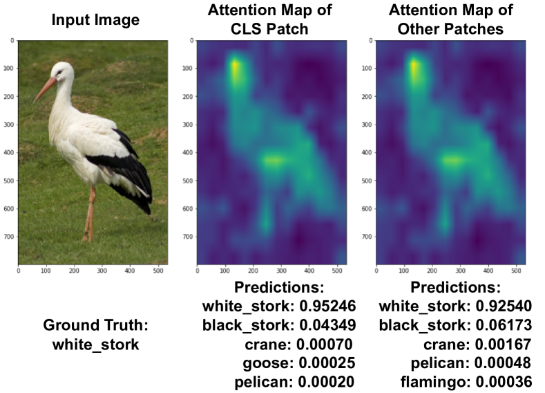
Figure 1: Illustration of uniform attention maps and predictive distributions produced by both the CLS patch and other image patches.

Among the efforts to enhance interpretability during the training process, we propose our novel interpretability-aware ViT (IA-ViT). Our inspiration comes from the observation that, in ViT models, the downstream classification tasks only utilize the embedding of the class (CLS) patch. In contrast, the feature embeddings of the image patches, which are learned using multi-layer MSA blocks, are underutilized and often neglected. Nevertheless, we have discovered that these neglected patch embeddings also contain discriminative features crucial for classification. Consequently, both the CLS patch and the image patches generate uniform attention maps and predictive distributions, as illustrated in Fig 1. In addition to qualitative confirmation, we also quantitatively substantiate this discovery in Table 1. Therefore, we suggest leveraging the valuable attributes of these image patches to generate explanations while utilizing the CLS patch embedding for prediction.

Table 1: Illustration of uniform attention maps and predictive distributions for 1000 samples drawn from the ImageNet dataset. $L_{2}$ denotes the average $L_{2}$ distance between the attention maps generated from the CLS and image patches. Top1 Consistency Rate (CR) illustrates the consistency rate between Top1 predictions produced using the CLS and image patches. Additionally, we employ Kendall’s $\tau$ Correlation to measure the Kendall rank correlation coefficient between these two sets of predictions.

$L_{2}$	CR (%)	Kendall’s $\tau$ Correlation
		Top2	Top3	Top4	Top5
0.0005655	0.95	0.79	0.64	0.52	0.42

Specifically, we consider that interpretation and prediction are two distinct but closely related tasks that can be simultaneously optimized during training. Therefore, aside from ViT’s inherent predictor, we introduce an interpreter into the model architecture as the interpretability-aware component. This interpreter comprises a single-head self-attention (SSA) mechanism and a linear head. SSA is employed to generate explanations through its attention weights, while the linear head maps the embeddings of image patches into the class dimension aiming to simulate the behavior of the predictor. In this way, IA-ViT preserves its high expressive capability with an interpretability-aware training objective while providing stable and faithful high-quality explanations.

We summarize our major contributions as follows: (1) We propose a novel IA-ViT architecture, which leverages the feature embeddings from the image patches beside the CLS patch to provide consistent, faithful, and high-quality explanations while maintaining high predictive performance. (2) Our novel developed interpretability-aware training objective has been demonstrated effective in enhancing the interpretability of IA-ViT. (3) We conduct a comprehensive comparison of our approach with several state-of-the-art methods, validating the quality and consistency of explanations generated by IA-ViT.

Related Works

Explainable AI

Depending on the method of explanation generation, general post hoc techniques in XAI can be broadly categorized into three groups: perturbation, approximation, and back-propagation. Perturbation methods, such as RISE (Petsiuk, Das, and Saenko 2018), Extremal Perturbations (Fong, Patrick, and Vedaldi 2019), and SHAP (Lundberg and Lee 2017), attempt to generate explanations by purposely perturbing the input images. However, these methods are often characterized by time-consuming and inefficient performance in practical applications. Approximation methods employ an external agent as the explainer for black-box models, such as LIME (Ribeiro, Singh, and Guestrin 2016) and FLINT (Parekh, Mozharovskyi, and d’Alché Buc 2021). Nonetheless, these approaches might not accurately capture the true predictive mechanism of the models. Back-propagation techniques apply the back-propagation scheme to generate gradients (Simonyan, Vedaldi, and Zisserman 2013; Zhou et al. 2016; Selvaraju et al. 2017; Li et al. 2023d) or gradient-related (Bach et al. 2015; Shrikumar, Greenside, and Kundaje 2017; Sundararajan, Taly, and Yan 2017; Shrikumar, Greenside, and Kundaje 2017; Pan, Li, and Zhu 2021; Qiang et al. 2022b; Li et al. 2023d) explanations. However, these methods may not faithfully reveal the decision-making process of trained models and might exhibit less reliable and robust (Adebayo et al. 2018; Kindermans et al. 2019; Agarwal et al. 2022).

Different from post hoc methods, alternative methods suggest making alterations to either the architectures (Frosst and Hinton 2017; Wu et al. 2018; Al-Shedivat, Dubey, and Xing 2020; Böhle, Fritz, and Schiele 2022), the loss functions (Zhang, Wu, and Zhu 2018; Chen, Bei, and Rudin 2020; Ismail, Corrada Bravo, and Feizi 2021), or both (Angelov and Soares 2020; Chen et al. 2019; Pan et al. 2020). Nevertheless, certain methods depend on factors like the presence of ground truth explanations (Ghaeini et al. 2019), the accessibility of annotations concerning incorrect explanations for specific inputs (Frosst and Hinton 2017), or external knowledge sources (Al-Shedivat, Dubey, and Xing 2020). Moreover, some interpretability constraints can potentially restrict the model’s expressive capabilities, which may lead to a trade-off with prediction performance.

Explanation Methods for ViTs

Motivated by the impressive success of Transformer architecture in NLP tasks (Vaswani et al. 2017), researchers have made efforts to extend the use of Transformer-based models to CV tasks (Dosovitskiy et al. 2020; Carion et al. 2020; Liu et al. 2021b; Touvron et al. 2021a; Yuan et al. 2021a; Zhou et al. 2021; Chu et al. 2021; Touvron et al. 2021b; Wang et al. 2022, 2021; Liu et al. 2022; Zhang et al. 2021; Guo et al. 2022). Meanwhile, researchers have been actively exploring ways to enhance their interpretability. One popular approach involves analyzing the attention weights of MSA in ViTs (Vaswani et al. 2017; Abnar and Zuidema 2020), however, the simple utilization may not provide reliable explanations (Serrano and Smith 2019; Qiang et al. 2022b). Other approaches have been proposed to reason the decision-making process of ViTs, such as using gradients (Chen et al. 2022; Gao et al. 2021; Gupta et al. 2022; Qiang et al. 2022b), attributions (Chefer, Gur, and Wolf 2021; Yuan et al. 2021b), and redundancy reduction (Pan et al. 2021). However, these post hoc methods still have the same limitations as discussed before.

Recently, some approaches have emerged to modify the ViT architecture to improve interpretability. The Concept-Transformer (Rigotti et al. 2021), for instance, exposes explanations of a ViT model’s output in terms of attention over user-defined high-level concepts. However, the usability of these methods largely depends on the presence of these human-annotated concepts. (Kim, Nam, and Ko 2022) proposed ViT-NeT, which interprets the decision-making process through a tree structure and prototypes with visual explanations. However, this method is not broadly applicable to various Transformer architectures and requires additional tree structures and external knowledge.

Different from existing works, we propose IA-ViT to directly improve its interpretability during the training process with the interpretability-aware objective. Moreover, our approach does not require external knowledge, such as pre-defined human-labeled concepts like Concept-Transformer (Rigotti et al. 2021) and additional complex architectures like ViT-NeT (Kim, Nam, and Ko 2022).

Preliminary

Overview of Vision Transformer

ViTs (Dosovitskiy et al. 2020) for image classification take a sequence of sliced patches from an image as input and model their long-range dependencies with Linear Patch Embedding and Positional Encoding, stacked MSA blocks, and Feed-Forward Networks (FFN). Formally, an input image is first split into a sequence of fixed-sized 2D patches $\mathbf{X}=[x_{1},x_{2},...,x_{N}]$ where N is the number of patches (e.g. $N=14\times 14$). These raw patches are then mapped into $d$-dimensional patch embeddings $\mathbf{Z}=[\mathbf{z}_{1},\mathbf{z}_{2},...,\mathbf{z}_{N}]$ with a linear layer. Positional embeddings $\mathbf{E}_{\mathrm{pos}}$ are also optionally added to patch embeddings to augment them with positional information. A learnable embedding $\mathbf{z}_{\mathrm{cls}}$ termed CLS patch is appended to the sequence of patch embeddings, which serves as the representation of the image. To summarize, the input to the first block is formulated as:

$$\mathbf{Z}=[\mathbf{z}_{\mathrm{cls}};\mathbf{z}_{1};\mathbf{z}_{2};\cdots;\mathbf{z}_{N}]+\mathbf{E}_{\mathrm{pos}},$$ (1)

where $\mathbf{z}\in\mathbb{R}^{d}$ and $\mathbf{E}_{\mathrm{pos}}\in\mathbb{R}^{(N+1)\times d}$.

Similar to Transformers (Vaswani et al. 2017), the backbone network of ViTs comprises $L$ blocks, where each block consists of an MSA and an FFN. Particularly, a single-head self-attention (SSA) is computed as:

$$\mathbf{A}=\mathrm{Softmax}\bigg{(}\frac{\mathbf{Q}\mathbf{K}^{T}}{\sqrt{d_{k}}}\bigg{)}\ \ \mathrm{and}\ \ \mathbf{S}=\mathbf{A}\mathbf{V},$$ (2)

where $\mathbf{Q},\mathbf{K},\mathbf{V}$ are query, key, and value matrices, which are projected from the same patch embeddings $\mathbf{Z}$ respectively, and $d_{k}$ is a scaling factor. For more effective attention on different representation sub-spaces, MSA concatenates the output from several SSAs as:

$$\mathbf{S}_{i,l}=\mathrm{SSA}(\mathbf{Z}_{l}W_{i,l}^{Q},\mathbf{Z}_{l}W_{i,l}^{K},\mathbf{Z}_{l}W_{i,l}^{V}),$$ (3)

where $W_{i,l}^{Q},W_{i,l}^{K},W_{i,l}^{V}$ are the parameter matrices in the $i$-th attention head of the $l$-th block, and $\mathbf{Z}_{l}$ denotes the input at the $l$-th block, and projects it with another parameter matrix $W_{l}^{O}$ as:

$$\mathrm{MSA}(\mathbf{Z}_{l})=[\mathbf{S}_{1,l};\cdots;\mathbf{S}_{H,l}]W_{l}^{O},$$ (4)

The output from MSA is then fed into FFN, a two-layer MLP, that produces the output of the block $\mathbf{Z}_{l+1}$. Residual connections are also applied on both MSA and FFN as:

$$\mathbf{Z}_{l}^{\prime}=\mathrm{MSA}(\mathbf{Z}_{l})+\mathbf{Z}_{l},$$ (5)

$$\mathbf{Z}_{l+1}=\mathrm{FFN}(\mathbf{Z}_{l}^{\prime})+\mathbf{Z}_{l}^{\prime}.$$ (6)

The final prediction is produced by a linear layer taking the CLS patch from the last block ($\mathbf{Z}_{L}^{0}$) as inputs.

Problem Formulation

In the context of a $\{(x_{i},y_{i})_{i=1}^{n}\}$, conventional post hoc explanation methods typically involve an explainer module $g$. This module takes the pre-trained model $f$ and an input $x$ to produce an explanation $e$ for the output $y$, formally: $g:f\times x\to e$. The space of potential explanations $e$ is usually determined by the specific explanation method in use. For example, a method employing saliency maps may define $e$ as normalized distributions indicating the importance of individual input elements, such as tokens and pixels.

In our work, we propose a general problem named Learning with Interpretation, which advocates that the interpretation task should be integrated into the training process of the model itself, as opposed to treating them as separate post hoc procedures. The core idea is to design a dedicated module, referred to as an interpreter, as an integral part of the model. This interpreter module relies on the predictor and is trained concurrently with it to furnish interpretability for the trained model. Essentially, this approach augments the model’s training process, encompassing not only the prediction objective but also an additional interpretability-aware objective.

Concretely, we design IA-ViT and a novel interpretability-aware training scheme to address the Learning with Interpretation problem, as shown in Fig 2. Our training framework for IA-ViT consists of three key objectives for the minimization of dedicated losses and regularization terms for the three functional modules: (1) A primary objective focusing on target prediction, aiming to minimize Cross-Entropy loss $\mathcal{L}_{\mathrm{pred}}$; (2) An additional objective centered on simulation, which encourages the interpreter to emulate the behavior of the predictor, and this is quantified as $\mathcal{L}_{\mathrm{kd}}$ using knowledge distillation; (3) An attention regularizer that aligns the attention weights form the MSA blocks with the interpretable SSA block $\mathcal{L}_{\mathrm{match}}$.

Our Approach - IA-ViT

IA-ViT Architecture

The proposed IA-ViT framework consists of three components: feature extractor $h$, predictor $f$, and interpreter $g$, as shown in Figure 2. The feature extractor, comprising a stack of $L$ MSA blocks, takes the input image $x$ and encodes it into $\mathbf{z}\in\mathbb{R}^{(N+1)\times d}$: $\mathbf{z}=h(x)$, where $N$ represents the number of image patches and $d$ is the embedding dimension. Subsequently, the predictor $f$ utilizes the feature embedding of the class token $\mathbf{z}^{0}$ from $\mathbf{z}$ to make predictions via a linear head: $\hat{y}_{\mathrm{pred}}=f(\mathbf{z}^{0})$. Conversely, the interpreter $g$ takes the remaining feature embeddings as inputs, processing them through an SSA block followed by a linear head to generate the prediction $\hat{y}_{\mathrm{int}}=g(\mathbf{z}^{1},\cdots,\mathbf{z}^{N})$. Thus, IA-ViT employs both the predictor and the interpreter to generate two highly simulated predictions $\hat{y}_{\mathrm{pred}}$ and $\hat{y}_{\mathrm{int}}$, while sharing the feature extractor $h$.

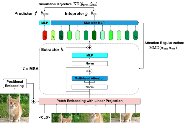
Figure 2: IA-ViT architecture consists of three major components: feature extractor, predictor, and interpreter. Both the predictor and the interpreter generate the class prediction for this cat image. KD is applied on the two logits in the simulation objective. The attention weights in SA and MSA are aligned via MMD during the training process for better explanations.

Interpretability of IA-ViT

The rationale behind incorporating an interpreter into IA-ViT is to enhance its interpretability by gaining insights into its prediction process. It is crucial that the interpreter faithfully replicates the behavior of the predictor, ensuring that its output closely aligns with the predictor’s output for a given input. Essentially, the predictor’s function is to convey the crucial aspects of the input that influence the final prediction, while the interpreter complements this by offering supplementary insights into the model’s decision-making process without altering the actual prediction.

Attention weights derived from MSA blocks can offer interpretable clues, but existing attention weights-based explanation methods (Serrano and Smith 2019; Abnar and Zuidema 2020) only provide post hoc explanations, which are limited in their ability to provide faithful explanations of the model’s decision-making process. To address this problem, the interpreter of IA-ViT applies an SSA mechanism, which dynamically aligns its attention weights with the discriminative patterns from the feature embeddings, to provide reliable and faithful explanations.

Given the input from the feature embeddings $\mathbf{Z}^{\prime}=[\mathbf{z}^{1},\cdots,\mathbf{z}^{N}]$, we obtain the projected key, query, and value as:

$$\mathbf{Q}=\mathbf{Z}^{\prime}\mathbf{W}^{Q},\ \ \mathbf{K}=\mathbf{Z}^{\prime}\mathbf{W}^{K},\ \ \mathrm{and}\ \ \mathbf{V}=\mathbf{Z}^{\prime}\mathbf{W}^{V},$$ (7)

where $\mathbf{W}^{Q}\in\mathbb{R}^{d\times d}$, $\mathbf{W}^{K}\in\mathbb{R}^{d\times d}$, and $\mathbf{W}^{V}\in\mathbb{R}^{d\times d}$ are trainable transform matrices. Note $\mathbf{Z}^{\prime}$ does not contain the feature embedding of the class patch $\mathbf{z}^{0}$. Based on SSA Eq.2, we obtain the attention weights $\mathbf{A}$ that characterize the amount of attention paid to each patch and the SSA features $\mathbf{S}$. According to Eq.2, we get $\|\mathbf{A}\|\leq 1$. Therefore, $\mathbf{S}$ is upper-bounded as:

$$\|\mathbf{S}\|=\|\mathbf{A}\|\ \|\mathbf{V}\|\cos(\mathbf{A},\mathbf{V})\leq\|\mathbf{V}\|.$$ (8)

When $\mathbf{S}$ is optimized, the attention weights $\mathbf{A}$ are proportional to $\mathbf{V}$. To achieve maximal output, $\mathbf{A}$ is driven to align with the discriminative features in $\mathbf{V}$. Therefore, $\mathbf{S}$ can only achieve this upper bound if all possible solutions of $\mathbf{v}\in\mathbf{V}$ are encoded as eigenvectors of $\mathbf{A}$. This maximization suggests with the attention weight $\mathbf{A}$, we will obtain an inherently explainable decomposition of input patterns.

Consequently, the SSA mechanism within the interpreter produces an attention map that inherently combines the contributions of discriminative input patterns with respect to the model’s outputs in an interpretable manner. This attention map offers more informative insights compared to the attention weights derived solely from the MSA blocks. It excels at emphasizing the specific input features that the model relied upon to make its predictions.

Learning with Interpretation

Within the framework of Learning with Interpretation, the interpreter’s goal extends beyond optimizing predictions alone; it also involves comprehending the rationale behind the model’s predictions concurrently. Therefore, IA-ViT adopts a joint training approach for the predictor and interpreter. This allows the interpreter to acquire insights that align with the predictions made by the predictor, ultimately enhancing the overall interpretability of the model. In this approach, the interpreter and predictor collaborate to produce accurate predictions while concurrently offering explanations for these predictions. This dual functionality can prove invaluable in various domains, including healthcare and finance, where the interpretability of learned models holds paramount importance.

Classification Objective

Given an input image $x$ with its corresponding label $y$, the final prediction is produced by the extractor and the predictor. Typically, the training process for the feature extractor and predictor involves minimizing the cross-entropy loss, which measures the disparity between the predicted probability distribution and the true labels. Formally, the cross-entropy loss is expressed as:

$$\mathcal{L}_{\mathrm{ce}}=-\frac{1}{n}\sum_{i=1}^{n}y_{i}\log(f(h(x_{i})),$$ (9)

where $f$ and $h$ are the predictor and feature extractor components of IA-ViT, respectively.

Simulation Objective

Knowledge distillation (KD) is a technique introduced in (Hinton et al. 2015), wherein a larger capacity teacher model is used to transfer its “dark knowledge" to a more compact student model. The goal of KD is to achieve a student model that not only inherits better qualities from the teacher but is also more efficient for inference due to its compact size. Recent studies (Tang et al. 2020) have highlighted the success of KD with several desirable effects, such as label smoothing from universal knowledge, injecting domain knowledge of class relationships to student’s output logit layer geometry, and gradient rescaling based on the teacher’s measurement of instance difficulty.

Our simulation objective is formulated to force the interpreter’s predictions to simulate the behavior of the predictor, as opposed to relying directly on ground truth labels but the soft labels generated by the predictor. Therefore, we apply KD as the simulation objective. In more detail, the logits generated by the predictor are denoted as $\mathbf{q}$, which is the output distribution computed by applying softmax over the outputs:

$$q_{i}=\frac{\exp(f(h(x))_{i})}{\sum_{j=1}^{C}\exp(f(h(x))_{j})},$$ (10)

where $C$ is the number of classes. To obtain a smooth distribution, the logits are usually scaled by a temperature factor $\tau>1$. Similarly, the interpreter produces a softened class probability distribution $\mathbf{p}$. Then we apply KD to these two probabilities:

$$\mathcal{L}_{\mathrm{kd}}=-\tau^{2}(\mathbf{q/\tau})\log(\mathbf{p}/\tau).$$ (11)

By optimizing $\mathcal{L}_{\mathrm{kd}}$, the interpreter is trained to predict the same class as the predictor with a high probability, which increases the fidelity of interpretations to the model’s outputs.

Attention Regularization

To further improve the interpretability of IA-ViT, we introduce an additional regularization term into the objective. This term serves to reduce the Maximum Mean Discrepancy (MMD) (Gretton et al. 2006, 2012) between the attention distribution of MSA in the feature extractor, denoted as $\boldsymbol{\alpha}_{\mathrm{ext}}$, and the attention distribution of the SSA in the interpreter, denoted as $\boldsymbol{\alpha}_{\mathrm{int}}$. This helps to ensure that the attention weights used by the feature extractor and the interpreter are generated from the same distribution, which can further improve the interpretability of the model.

Since MSA in the feature extractor employs multi-headed attention with multiple different attention vectors in each block, we aggregate these attentions by summing up the attention from the class token to other tokens in the last layer. This summation is then averaged across all attention heads to get $\boldsymbol{\alpha}_{\mathrm{ext}}$, i.e., $\mathbf{A}_{0}$. In contrast, $\boldsymbol{\alpha}_{\mathrm{int}}$ can be directly extracted from SSA in the interpreter. MMD compares the sample statistics between $\boldsymbol{\alpha}_{\mathrm{int}}$ and $\boldsymbol{\alpha}_{\mathrm{ext}}$, and if the discrepancy is small, $\boldsymbol{\alpha}_{\mathrm{int}}$ and $\boldsymbol{\alpha}_{\mathrm{ext}}$ are then likely to follow the same distribution. Thus, the attention regularizer is formulated as:

$$\mathcal{L}_{\mathrm{reg}}=\mathrm{MMD}(\boldsymbol{\alpha}_{\mathrm{int}},\boldsymbol{\alpha}_{\mathrm{ext}}).$$ (12)

We conduct an in-depth analysis of this attention regularization to obtain a more comprehensive understanding of its positive impacts on the IA-ViT training process. Using the kernel trick, the empirical estimate of $M$ can be obtained as:

$$M= \bigg{[}\frac{1}{n^{2}}\sum_{i,j=1}^{n}\mathcal{K}(\alpha^{\mathrm{i}}_{i},\alpha^{\mathrm{i}}_{j})+\frac{1}{n^{2}}\sum_{i,j=1}^{n}\mathcal{K}(\alpha^{\mathrm{e}}_{i},\alpha^{\mathrm{e}}_{j})$$ (13)

$$-\frac{2}{n^{2}}\sum_{i=1}^{n}\sum_{j=1}^{n}\mathcal{K}(\alpha^{\mathrm{i}}_{i},\alpha^{\mathrm{e}}_{j})\bigg{]}^{1/2},$$

where $\mathcal{K}(\cdot,\cdot)$ is a kernel function, and $n$ is the number of samples. Moreover, for notational simplicity we use $\boldsymbol{\alpha}^{\mathrm{e}}$ and $\boldsymbol{\alpha}^{\mathrm{i}}$ to denote $\boldsymbol{\alpha}_{\mathrm{ext}}$ and $\boldsymbol{\alpha}_{\mathrm{int}}$, respectively. (Gretton et al. 2006) showed that if $\mathcal{K}$ is a characteristic kernel, then $\mathrm{MMD}(\boldsymbol{\alpha}^{e},\boldsymbol{\alpha}^{i})$ = 0 asymptotically if and only $\boldsymbol{\alpha}^{\mathrm{i}}$ and $\boldsymbol{\alpha}^{\mathrm{e}}$ are generated from the same distribution. A typical choice of $\mathcal{K}$ is the Gaussian kernel with bandwidth parameter $\sigma$:

$$\mathcal{K}(x,y)=\exp\Big{(}\frac{-\|x-y\|^{2}}{\sigma}\Big{)}.$$ (14)

With the Gaussian kernel, minimizing MMD is equivalent to matching all orders of moments of the two distributions.

Inspired by the idea of (Li et al. 2023c), we further analyze the effect of MMD on our regularization. Since $\boldsymbol{\alpha}^{\mathrm{i}}$ and $\boldsymbol{\alpha}^{\mathrm{e}}$ are symmetric in MMD, we only present the attention weights of $\boldsymbol{\alpha}^{\mathrm{i}}$ here without loss of generality. We first formulate the gradient of the regularization loss with respect to $\boldsymbol{\alpha}^{\mathrm{i}}$ as:

$$\nabla_{\alpha_{i}^{\mathrm{i}}}M=\frac{2}{\sqrt{M}}\nabla_{\alpha^{\mathrm{i}}}\bigg{[} \frac{1}{n^{2}}\sum_{j=1}^{n}\mathcal{K}(\alpha^{\mathrm{i}}_{i},\alpha^{\mathrm{i}}_{j})$$ (15)

$$-\frac{2}{n^{2}}\sum_{j=1}^{n}\mathcal{K}(\alpha^{\mathrm{i}}_{i},\alpha^{\mathrm{e}}_{j})\bigg{]}.$$

The gradient with respect to $x$ for Gaussian kernel $\mathcal{K}$ is:

$$\nabla_{x}\mathcal{K}(x,y)=-2\exp\bigg{(}\frac{-\|x-y\|^{2}}{\sigma}\bigg{)}\frac{x-y}{\sigma}.$$ (16)

Since $\sigma$ here is data-dependent and treated as a hyperparameter, it is not back propagated in the training process and practice set as the median of sample pairwise distances. We thus get

$$\nabla_{\alpha_{i}^{\mathrm{i}}}M= -\frac{2}{\sqrt{M}}\bigg{[}\frac{1}{n^{2}}\sum_{j=1}^{n}\exp\bigg{(}-\frac{\|\alpha^{\mathrm{i}}_{i}-\alpha^{\mathrm{i}}_{j}\|^{2}}{\sigma}\bigg{)}\frac{\alpha^{\mathrm{i}}_{i}-\alpha^{\mathrm{i}}_{j}}{\sigma}$$ (17)

$$-\frac{2}{n^{2}}\sum_{j=1}^{n}\exp\bigg{(}-\frac{\|\alpha^{\mathrm{i}}_{i}-\alpha^{\mathrm{e}}_{j}\|^{2}}{\sigma}\bigg{)}\frac{\alpha^{\mathrm{i}}_{i}-\alpha^{\mathrm{e}}_{j}}{\sigma}\bigg{]},$$

by the linearity of the gradient operator. We notice that for function $g_{a}(x)=\exp({-x^{2}/a})x/a$ ($a$ is some constant), $g_{a}(x)\to 0$ exponentially as $x\to\infty$. We further achieve

$$\|\nabla_{\alpha^{\mathrm{i}}}M\|\leq\frac{2}{\sqrt{M}}\left[\frac{1}{n^{2}}\sum_{j=1}^{n}g_{\sigma}(\|\alpha^{\mathrm{i}}_{i}-\alpha^{\mathrm{i}}_{j}\|)\right.$$ (18)

$$\left.+\frac{2}{n^{2}}\sum_{j=1}^{n}g_{\sigma}(\|\alpha^{\mathrm{i}}_{i}-\alpha^{\mathrm{e}}_{j}\|)\right]$$

using the triangle inequality for the $L_{2}$ norm for fixed $\sigma$. $\sqrt{M}$ here is a constant for all samples within the training mini-batch.

We observe that when $\alpha^{\mathrm{i}}$ deviates significantly away from the majority of samples of the same class, i.e., noisy samples or outliers, $\|\alpha^{\mathrm{i}}_{i}-\alpha^{\mathrm{i}}_{j}\|$ and $\|\alpha^{\mathrm{i}}_{i}-\alpha^{\mathrm{e}}_{j}\|$ are large, the magnitude of its gradient in the regularization loss diminishes from Eq.18. More specifically, $\alpha^{\mathrm{i}}$ has negligible impact on the regularization term. On the other hand, training IA-ViT with the regularization term promotes the alignment of attention weights representations of samples that stay close in attention weights distribution. The attention weights deviating from the majority are likely low-density or even outliers from the distribution perspective. Overall, such behavior of the regularization loss implies that it can help IA-ViT better capture information from high-density areas and reduce the distraction of low-density areas in learning feature representations on the data manifold, as shown in Figure 4.

Overall Objective

Combining all of these objectives, the overall training objective is formulated as the weighted sum of $\mathcal{L}_{\mathrm{ce}}$, $\mathcal{L}_{\mathrm{kd}}$, and $\mathcal{L}_{\mathrm{reg}}$. Formally, it is expressed as::

$$\mathcal{L}=\beta\mathcal{L}_{\mathrm{ce}}+(1-\beta)(\mathcal{L}_{\mathrm{kd}}+\mathcal{L}_{\mathrm{reg}}),$$ (19)

where $\beta\in(0,1)$ is a hyperparameter that balances the contributions of each term.

Experiment Settings

Datasets

We evaluate the performance of IA-ViT using various benchmark datasets tailored for image classification tasks, including CIFAR10 (Krizhevsky, Hinton et al. 2009), STL10 (Coates, Ng, and Lee 2011), Dog and Cat (Elson et al. 2007), and CelebA (Liu et al. 2018) (specifically for hair color prediction). Dataset statistics are presented in Table 2. The images from these datasets are upsampled to a standard resolution of $224\times 224$ for both training and testing.

Table 2: Dataset Statistics

Datasets	Training Size	Test Size	Class Numbers
CIFAR10	50,000	10,000	10
STL10	5,000	8,0000	10
Dog&Cat	20,000	5,000	2
CelebA	10,000	3,000	2

Model Architectures

We employ the vanilla ViT-B/16 architecture (Dosovitskiy et al. 2020) as the transformer backbone for our model. Specifically, we use the base version with patches of size $16\times 16$, which was exclusively pre-trained on the ImageNet-21k dataset. This backbone consists of 12 stacked MSA blocks, each containing 12 attention heads. The model utilizes a total of 196 patches, and each patch is flattened and projected into a 768-dimensional vector. Positional embeddings are added to these patch embeddings, and the resulting embeddings are then processed by the feature extractor. Following this, the predictor utilizes the feature embeddings of the class patch and passes them through two fully-connected layers and a softmax layer to produce logits for prediction. In contrast, the interpreter operates on the feature embeddings from other image patches. It employs a single SSA block, followed by two fully-connected layers and a softmax layer, to generate logit scores for interpretation.

Implementation Details

Both the ViT and IA-ViT models are trained using Stochastic Gradient Descent (SGD) with a momentum parameter of 0.9. The training process begins with an initial learning rate of 3e-2, lasting for 200 epochs. A constant batch size of 64 is maintained, and gradient clipping is applied to ensure that the global norm does not exceed 1. A cosine decay learning rate schedule with a linear warm-up phase is implemented. The values for the temperature parameter ($\tau$) in $\mathcal{L}_{\mathrm{kd}}$ and the hyperparameter ($\beta$) in $\mathcal{L}$ are adjusted flexibly to strike a balance between achieving optimal predictive performance and interpretability, tailored to the specific datasets. The model with the highest accuracy on the validation sets is ultimately chosen as the final model.

Baseline Explanation Methods

Rollout (Abnar and Zuidema 2020) is an explanation method that relies on attention mechanisms to identify the most crucial input patches for generating an output in Transformer-based models. AttGrads (Barkan et al. 2021) is an explanation method that utilizes gradients of the attention weights to pinpoint the most significant patches. In this context, experiments have been conducted to compare and evaluate the relative performance and effectiveness of these two methods in providing explanations for the models under consideration.

Evaluation Metrics

To evaluate the IA-ViT model’s performance comprehensively, we report accuracy metrics for both the predictor and the interpreter. We employ attribution maps, which are visual representations highlighting the input pixels considered significant or insignificant in relation to a predicted label. This approach is used for a qualitative evaluation of the explanation quality (Nguyen, Kim, and Nguyen 2021). Furthermore, we utilize insertion score and deletion score as quantitative evaluation metrics. In the first round of experiments, we replace the most important pixels with black pixels, following the approach of (Petsiuk, Das, and Saenko 2018). In the second round, we replace these pixels with Gaussian-blurred pixels, as per (Sturmfels, Lundberg, and Lee 2020). We report the average performance across both rounds of experiments. Since both deletion and insertion scores can be influenced by shifts in distribution when pixels are removed or added, we employ the difference between the insertion and deletion scores as an additional metric for comparison (Shah, Jain, and Netrapalli 2021). Focusing on their relative differences helps to mitigate the impact of these distribution shifts (Hooker et al. 2019).

Results and Discussion

Model Performance Evaluations

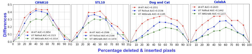
Figure 3: Quantitative Performance Comparison in terms of differences between insertion and deletion scores.

Table 3 presents a performance comparison between IA-ViT and the vanilla ViT models. It is important to highlight that the IA-ViT models’ final predictions rely on the predictor’s outputs. We apply performance drop rate (PDR) to evaluate the performance degradation, formally:

$$\mathrm{PDR}=1-\frac{\mathrm{Accuracy}_{\mathrm{IA-ViT}}}{\mathrm{Accuracy}_{\mathrm{ViT}}}.$$ (20)

The average PDR among these datasets is 1.16%, which indicates that there is no substantial decrease in accuracy when employing the IA-ViT model with its integrated interpreter.

Table 3: Comparison of the classification accuracies of the ViT and IA-ViT models. PDR refers to the performance drop rate.

Datasets	ViT	IA-ViT
		Predictor	Interpreter	PDR (%)
CIFAR10	98.93	97.51	97.24	1.43
STL10	99.31	97.73	95.42	1.59
Dog&Cat	99.72	98.82	97.76	0.90
CelebA	96.87	96.16	96.09	0.73

Quantitative Evaluations

Table 4: Quantitative evaluation using deletion and insertion scores. The deletion score is the lower the better, while the insertion score is the higher the better. The best results are in bold.

Datasets	Metrics	ViT		IA-ViT
		Rollout	AttGrads	Atts
CIFAR10	Deletion$\downarrow$	0.3817	0.3036	0.2479
	Insertion$\uparrow$	0.6141	0.5583	0.7082
STL10	Deletion	0.3874	0.4124	0.3254
	Insertion	0.5967	0.5546	0.6436
Dog&Cat	Deletion	0.6785	0.7354	0.6232
	Insertion	0.8322	0.7921	0.8783
CelebA	Deletion	0.7260	0.7536	0.5977
	Insertion	0.8275	0.8123	0.8719

The quantitative evaluations shown in Table 4 demonstrate that the attention weights (Atts) from the interpreter in IA-ViT outperform the Rollout and AttGrads methods for ViT in terms of deletion and insertion scores across all datasets. This further illustrates that the explanations generated by the interpreter of IA-ViT clearly capture the most important discriminative pixels or patches for the image classification tasks. Similarly, the results of the difference between insertion and deletion scores across a varying percentage of deleted/inserted pixes, as shown in Figure 3, clearly show that the form of the interpreter in IA-ViT outperforms the other baselines in terms of Area Under the Curve (AUC) among all tasks. These quantitative evaluations collectively provide compelling evidence of IA-ViT’s superior interpretability compared to the post hoc methods designed for ViT.

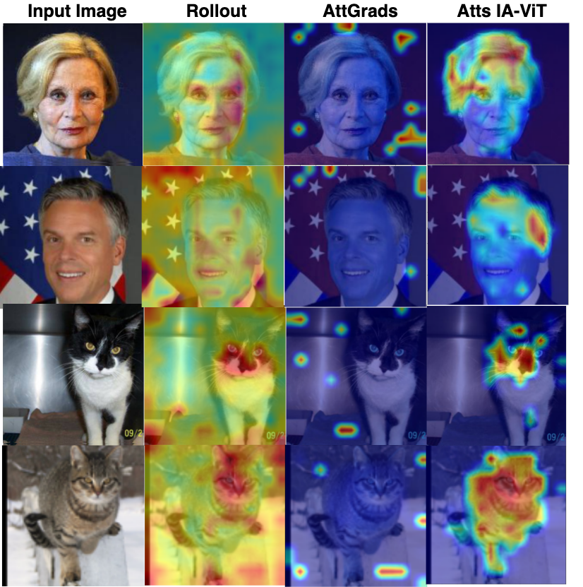
Figure 4: Examples of attribution maps obtained by post hoc methods Rollout and AttGrads for ViT and attention weights of IA-ViT.

Qualitative Evaluations

The examples provided in Figure 4 vividly illustrate the superior quality of the attribution maps produced by IA-ViT’s interpreter when compared to the post hoc methods Rollout and AttGrads designed for ViT. A key observation from this figure is that the heatmaps generated by IA-ViT’s interpreter exhibit more focused attention on the target objects, whereas the heatmaps generated by Rollout are dispersed across both the background and class entities. In contrast, AttGrads produces heatmaps that primarily highlight areas unrelated to the target. It’s essential to emphasize that the results depicted in Figure 4 are representative of the typical outcomes observed in our experiments and have not been cheery-picked.

Additionally, these qualitative examples also highlight the effectiveness of the attention regularization utilized in the training objective, as discussed in Section Attention Regularization. IA-ViT models possess the capability to extract information from regions with high information density while mitigating the influence of regions with low information density during the feature learning process. Therefore, the interpreter produces high-quality explanations that densely emphasize the target object. This is clearly evident in Figure 4, where the heatmaps generated by the interpreter distinctly highlight the target objects (e.g., hair, dog, cat) while disregarding the background or other irrelevant noise. In contrast, the explanations generated by the Rollout and AttGrads methods merely accentuate certain irrelevant areas and fail to capture the precise shape of the target objects.

Fairness Learning

Table 5: Fairness and accuracy comparison for ViT and IA-ViT over the target (Y) and sensitive (S) on the CelebA dataset.

Models	$Y$: Hair Color  $S$: Gender
	ACC$\uparrow$	DP$\downarrow$	EO$\downarrow$
ViT	96.89	12.95	8.69
IA-ViT	96.59	9.81	5.76

The examples from the CelebA dataset, specifically the hair color prediction task, illustrate that the attribution maps produced by the interpreter of IA-ViT concentrate intensely on the hair region, prioritizing it over other facial features. This is evident in the first two rows of Figure 4. On the contrary, the explanations generated by the Rollout method for the ViT model demonstrate that the ViT models tend to learn some spurious features that might be related to the sensitive attribute (in this case, gender) but not the real feature that is relevant to the hair color prediction.

These observations have motivated us to evaluate the performance of IA-ViT in the context of fairness learning (Qiang et al. 2022a; Wan et al. 2023; Qiang et al. 2023). Specifically, we employ two commonly used fairness metrics: demographic parity (DP) and equality of odds (EO) for fairness evaluation. DP measures whether the true positive rates are equal across all groups categorized by a sensitive label $s$ (e.g., gender), particularly comparing the vulnerable minority group ($s=0$) to others ($s=1$). It is formally defined as:

$$\mathrm{DP}=\mathrm{TPR}_{s=1}-\mathrm{TPR}_{s=0}.$$ (21)

EO, on the other hand, is used to examine the disparities in both the true positive rates and the false positive rates within the vulnerable group compared to others:

$$\mathrm{EO}=\frac{1}{2}[\mathrm{TPR}_{s=1}-\mathrm{TPR}_{s=0}]+\frac{1}{2}[\mathrm{FPR}_{s=1}-\mathrm{FPR}_{s=0}].$$ (22)

Table 5 demonstrates that the IA-ViT model outperforms the ViT model in both fairness metrics. The reduced DP and EO values indicate that IA-ViT’s training effectively mitigates bias, resulting in a fairer model. This further demonstrates the effectiveness of our interpretability-aware training, which indeed extracts “real" features rather than spurious ones.

Conclusion

In this work, we propose an interpretability-aware variant of the Vision Transformer (ViT) named IA-ViT. Our motivation stems from the consistent predictive distributions and attention maps generated by both the CLS patch and image patches in ViT models. IA-ViT consists of three major components: a feature extractor, a predictor, and an interpreter. By training the predictor and interpreter jointly, we enable the interpreter to acquire explanations that align with the predictor’s predictions, enhancing overall interpretability. As a result, IA-ViT not only maintains strong predictive performance but also delivers consistent, reliable, and high-quality explanations. Extensive experiments validate the efficacy of our interpretability-aware training approach in improving interpretability across various benchmark datasets when compared to several baseline explanation methods.

References

- Abnar and Zuidema (2020) Abnar, S.; and Zuidema, W. 2020. Quantifying attention flow in transformers. arXiv preprint arXiv:2005.00928.
- Adebayo et al. (2018) Adebayo, J.; Gilmer, J.; Muelly, M.; Goodfellow, I.; Hardt, M.; and Kim, B. 2018. Sanity checks for saliency maps. Advances in neural information processing systems, 31.
- Agarwal et al. (2022) Agarwal, C.; Saxena, E.; Krishna, S.; Pawelczyk, M.; Johnson, N.; Puri, I.; Zitnik, M.; and Lakkaraju, H. 2022. OpenXAI: Towards a Transparent Evaluation of Model Explanations. arXiv preprint arXiv:2206.11104.
- Al-Shedivat, Dubey, and Xing (2020) Al-Shedivat, M.; Dubey, A.; and Xing, E. P. 2020. Contextual Explanation Networks. J. Mach. Learn. Res., 21: 194–1.
- Alvarez-Melis and Jaakkola (2018) Alvarez-Melis, D.; and Jaakkola, T. S. 2018. On the robustness of interpretability methods. arXiv preprint arXiv:1806.08049.
- Angelov and Soares (2020) Angelov, P.; and Soares, E. 2020. Towards explainable deep neural networks (xDNN). Neural Networks, 130: 185–194.
- Arrieta et al. (2020) Arrieta, A. B.; Díaz-Rodríguez, N.; Del Ser, J.; Bennetot, A.; Tabik, S.; Barbado, A.; García, S.; Gil-López, S.; Molina, D.; Benjamins, R.; et al. 2020. Explainable Artificial Intelligence (XAI): Concepts, taxonomies, opportunities and challenges toward responsible AI. Information fusion, 58: 82–115.
- Bach et al. (2015) Bach, S.; Binder, A.; Montavon, G.; Klauschen, F.; Müller, K.-R.; and Samek, W. 2015. On pixel-wise explanations for non-linear classifier decisions by layer-wise relevance propagation. PloS one, 10(7): e0130140.
- Barkan et al. (2021) Barkan, O.; Hauon, E.; Caciularu, A.; Katz, O.; Malkiel, I.; Armstrong, O.; and Koenigstein, N. 2021. Grad-SAM: Explaining Transformers via Gradient Self-Attention Maps. In Proceedings of the 30th ACM International Conference on Information & Knowledge Management, 2882–2887.
- Böhle, Fritz, and Schiele (2022) Böhle, M.; Fritz, M.; and Schiele, B. 2022. B-Cos networks: alignment is all we need for interpretability. In Proceedings of the IEEE/CVF Conference on Computer Vision and Pattern Recognition, 10329–10338.
- Carion et al. (2020) Carion, N.; Massa, F.; Synnaeve, G.; Usunier, N.; Kirillov, A.; and Zagoruyko, S. 2020. End-to-end object detection with transformers. In European conference on computer vision, 213–229. Springer.
- Chefer, Gur, and Wolf (2021) Chefer, H.; Gur, S.; and Wolf, L. 2021. Transformer interpretability beyond attention visualization. In Proceedings of the IEEE/CVF Conference on Computer Vision and Pattern Recognition, 782–791.
- Chen et al. (2019) Chen, C.; Li, O.; Tao, D.; Barnett, A.; Rudin, C.; and Su, J. K. 2019. This looks like that: deep learning for interpretable image recognition. Advances in neural information processing systems, 32.
- Chen, Bei, and Rudin (2020) Chen, Z.; Bei, Y.; and Rudin, C. 2020. Concept whitening for interpretable image recognition. Nature Machine Intelligence, 2(12): 772–782.
- Chen et al. (2022) Chen, Z.; Wang, C.; Wang, Y.; Jiang, G.; Shen, Y.; Tai, Y.; Wang, C.; Zhang, W.; and Cao, L. 2022. Lctr: On awakening the local continuity of transformer for weakly supervised object localization. In Proceedings of the AAAI Conference on Artificial Intelligence, volume 36, 410–418.
- Chu et al. (2021) Chu, X.; Tian, Z.; Wang, Y.; Zhang, B.; Ren, H.; Wei, X.; Xia, H.; and Shen, C. 2021. Twins: Revisiting the design of spatial attention in vision transformers. Advances in Neural Information Processing Systems, 34: 9355–9366.
- Coates, Ng, and Lee (2011) Coates, A.; Ng, A.; and Lee, H. 2011. An analysis of single-layer networks in unsupervised feature learning. In Proceedings of the fourteenth international conference on artificial intelligence and statistics, 215–223. JMLR Workshop and Conference Proceedings.
- Devlin et al. (2018) Devlin, J.; Chang, M.-W.; Lee, K.; and Toutanova, K. 2018. Bert: Pre-training of deep bidirectional transformers for language understanding. arXiv preprint arXiv:1810.04805.
- Dosovitskiy et al. (2020) Dosovitskiy, A.; Beyer, L.; Kolesnikov, A.; Weissenborn, D.; Zhai, X.; Unterthiner, T.; Dehghani, M.; Minderer, M.; Heigold, G.; Gelly, S.; et al. 2020. An image is worth 16x16 words: Transformers for image recognition at scale. arXiv preprint arXiv:2010.11929.
- Elson et al. (2007) Elson, J.; Douceur, J. R.; Howell, J.; and Saul, J. 2007. Asirra: a CAPTCHA that exploits interest-aligned manual image categorization. CCS, 7: 366–374.
- Fong, Patrick, and Vedaldi (2019) Fong, R.; Patrick, M.; and Vedaldi, A. 2019. Understanding deep networks via extremal perturbations and smooth masks. In Proceedings of the IEEE/CVF international conference on computer vision, 2950–2958.
- Frosst and Hinton (2017) Frosst, N.; and Hinton, G. 2017. Distilling a neural network into a soft decision tree. arXiv preprint arXiv:1711.09784.
- Gao et al. (2021) Gao, W.; Wan, F.; Pan, X.; Peng, Z.; Tian, Q.; Han, Z.; Zhou, B.; and Ye, Q. 2021. Ts-cam: Token semantic coupled attention map for weakly supervised object localization. In Proceedings of the IEEE/CVF International Conference on Computer Vision, 2886–2895.
- Ghaeini et al. (2019) Ghaeini, R.; Fern, X. Z.; Shahbazi, H.; and Tadepalli, P. 2019. Saliency learning: Teaching the model where to pay attention. arXiv preprint arXiv:1902.08649.
- Gretton et al. (2006) Gretton, A.; Borgwardt, K.; Rasch, M.; Schölkopf, B.; and Smola, A. 2006. A kernel method for the two-sample-problem. Advances in neural information processing systems, 19.
- Gretton et al. (2012) Gretton, A.; Borgwardt, K. M.; Rasch, M. J.; Schölkopf, B.; and Smola, A. 2012. A kernel two-sample test. The Journal of Machine Learning Research, 13(1): 723–773.
- Guo et al. (2022) Guo, J.; Han, K.; Wu, H.; Tang, Y.; Chen, X.; Wang, Y.; and Xu, C. 2022. Cmt: Convolutional neural networks meet vision transformers. In Proceedings of the IEEE/CVF Conference on Computer Vision and Pattern Recognition, 12175–12185.
- Gupta et al. (2022) Gupta, S.; Lakhotia, S.; Rawat, A.; and Tallamraju, R. 2022. ViTOL: Vision Transformer for Weakly Supervised Object Localization. In Proceedings of the IEEE/CVF Conference on Computer Vision and Pattern Recognition, 4101–4110.
- Hao et al. (2021) Hao, Y.; Dong, L.; Wei, F.; and Xu, K. 2021. Self-attention attribution: Interpreting information interactions inside transformer. In Proceedings of the AAAI Conference on Artificial Intelligence, volume 35, 12963–12971.
- Hinton et al. (2015) Hinton, G.; Vinyals, O.; Dean, J.; et al. 2015. Distilling the knowledge in a neural network. arXiv preprint arXiv:1503.02531, 2(7).
- Hooker et al. (2019) Hooker, S.; Erhan, D.; Kindermans, P.-J.; and Kim, B. 2019. A benchmark for interpretability methods in deep neural networks. Advances in neural information processing systems, 32.
- Ismail, Corrada Bravo, and Feizi (2021) Ismail, A. A.; Corrada Bravo, H.; and Feizi, S. 2021. Improving deep learning interpretability by saliency guided training. Advances in Neural Information Processing Systems, 34: 26726–26739.
- Kim and Canny (2017) Kim, J.; and Canny, J. 2017. Interpretable learning for self-driving cars by visualizing causal attention. In Proceedings of the IEEE international conference on computer vision, 2942–2950.
- Kim, Nam, and Ko (2022) Kim, S.; Nam, J.; and Ko, B. C. 2022. Vit-net: Interpretable vision transformers with neural tree decoder. In International Conference on Machine Learning, 11162–11172. PMLR.
- Kindermans et al. (2019) Kindermans, P.-J.; Hooker, S.; Adebayo, J.; Alber, M.; Schütt, K. T.; Dähne, S.; Erhan, D.; and Kim, B. 2019. The (un) reliability of saliency methods. In Explainable AI: Interpreting, Explaining and Visualizing Deep Learning, 267–280. Springer.
- Krizhevsky, Hinton et al. (2009) Krizhevsky, A.; Hinton, G.; et al. 2009. Learning multiple layers of features from tiny images.
- Li et al. (2022) Li, C.; Bagher-Ebadian, H.; Goddla, V.; Chetty, I. J.; and Zhu, D. 2022. FocalUNETR: A Focal Transformer for Boundary-aware Segmentation of CT Images. arXiv preprint arXiv:2210.03189.
- Li et al. (2023a) Li, C.; Khanduri, P.; Qiang, Y.; Sultan, R. I.; Chetty, I.; and Zhu, D. 2023a. Auto-Prompting SAM for Mobile Friendly 3D Medical Image Segmentation. arXiv preprint arXiv:2308.14936.
- Li et al. (2023b) Li, X.; Bagher-Ebadian, H.; Gardner, S.; Kim, J.; Elshaikh, M.; Movsas, B.; Zhu, D.; and Chetty, I. J. 2023b. An uncertainty-aware deep learning architecture with outlier mitigation for prostate gland segmentation in radiotherapy treatment planning. Medical physics, 50(1): 311–322.
- Li et al. (2023c) Li, X.; Li, X.; Pan, D.; Qiang, Y.; and Zhu, D. 2023c. Learning compact features via in-training representation alignment. In Proceedings of the AAAI Conference on Artificial Intelligence, volume 37, 8675–8683.
- Li et al. (2023d) Li, X.; Pan, D.; Li, C.; Qiang, Y.; and Zhu, D. 2023d. Negative Flux Aggregation to Estimate Feature Attributions. arXiv preprint arXiv:2301.06989.
- Liu et al. (2021a) Liu, F.; Wu, X.; Ge, S.; Ren, X.; Fan, W.; Sun, X.; and Zou, Y. 2021a. Dimbert: learning vision-language grounded representations with disentangled multimodal-attention. ACM Transactions on Knowledge Discovery from Data (TKDD), 16(1): 1–19.
- Liu et al. (2021b) Liu, Z.; Lin, Y.; Cao, Y.; Hu, H.; Wei, Y.; Zhang, Z.; Lin, S.; and Guo, B. 2021b. Swin transformer: Hierarchical vision transformer using shifted windows. In Proceedings of the IEEE/CVF International Conference on Computer Vision, 10012–10022.
- Liu et al. (2018) Liu, Z.; Luo, P.; Wang, X.; and Tang, X. 2018. Large-scale celebfaces attributes (celeba) dataset. Retrieved August, 15(2018): 11.
- Liu et al. (2022) Liu, Z.; Ning, J.; Cao, Y.; Wei, Y.; Zhang, Z.; Lin, S.; and Hu, H. 2022. Video swin transformer. In Proceedings of the IEEE/CVF Conference on Computer Vision and Pattern Recognition, 3202–3211.
- Lundberg and Lee (2017) Lundberg, S. M.; and Lee, S.-I. 2017. A unified approach to interpreting model predictions. Advances in neural information processing systems, 30.
- Nguyen, Kim, and Nguyen (2021) Nguyen, G.; Kim, D.; and Nguyen, A. 2021. The effectiveness of feature attribution methods and its correlation with automatic evaluation scores. Advances in Neural Information Processing Systems, 34: 26422–26436.
- Pan et al. (2021) Pan, B.; Panda, R.; Jiang, Y.; Wang, Z.; Feris, R.; and Oliva, A. 2021. IA-RED: Interpretability-Aware Redundancy Reduction for Vision Transformers. Advances in Neural Information Processing Systems, 34: 24898–24911.
- Pan et al. (2020) Pan, D.; Li, X.; Li, X.; and Zhu, D. 2020. Explainable recommendation via interpretable feature mapping and evaluation of explainability. arXiv preprint arXiv:2007.06133.
- Pan, Li, and Zhu (2021) Pan, D.; Li, X.; and Zhu, D. 2021. Explaining deep neural network models with adversarial gradient integration. In Thirtieth International Joint Conference on Artificial Intelligence (IJCAI).
- Parekh, Mozharovskyi, and d’Alché Buc (2021) Parekh, J.; Mozharovskyi, P.; and d’Alché Buc, F. 2021. A framework to learn with interpretation. Advances in Neural Information Processing Systems, 34: 24273–24285.
- Petsiuk, Das, and Saenko (2018) Petsiuk, V.; Das, A.; and Saenko, K. 2018. Rise: Randomized input sampling for explanation of black-box models. arXiv preprint arXiv:1806.07421.
- Qiang et al. (2022a) Qiang, Y.; Li, C.; Brocanelli, M.; and Zhu, D. 2022a. Counterfactual interpolation augmentation (CIA): A unified approach to enhance fairness and explainability of DNN. In Proceedings of the Thirty-First International Joint Conference on Artificial Intelligence, IJCAI, 732–739.
- Qiang et al. (2023) Qiang, Y.; Li, C.; Khanduri, P.; and Zhu, D. 2023. Fairness-aware Vision Transformer via Debiased Self-Attention. arXiv preprint arXiv:2301.13803.
- Qiang et al. (2022b) Qiang, Y.; Pan, D.; Li, C.; Li, X.; Jang, R.; and Zhu, D. 2022b. AttCAT: Explaining Transformers via Attentive Class Activation Tokens. In Advances in Neural Information Processing Systems.
- Ribeiro, Singh, and Guestrin (2016) Ribeiro, M. T.; Singh, S.; and Guestrin, C. 2016. " Why should i trust you?" Explaining the predictions of any classifier. In Proceedings of the 22nd ACM SIGKDD international conference on knowledge discovery and data mining, 1135–1144.
- Rigotti et al. (2021) Rigotti, M.; Miksovic, C.; Giurgiu, I.; Gschwind, T.; and Scotton, P. 2021. Attention-based Interpretability with Concept Transformers. In International Conference on Learning Representations.
- Ross, Hughes, and Doshi-Velez (2017) Ross, A. S.; Hughes, M. C.; and Doshi-Velez, F. 2017. Right for the right reasons: Training differentiable models by constraining their explanations. arXiv preprint arXiv:1703.03717.
- Samek et al. (2019) Samek, W.; Montavon, G.; Vedaldi, A.; Hansen, L. K.; and Müller, K.-R. 2019. Explainable AI: interpreting, explaining and visualizing deep learning, volume 11700. Springer Nature.
- Selvaraju et al. (2017) Selvaraju, R. R.; Cogswell, M.; Das, A.; Vedantam, R.; Parikh, D.; and Batra, D. 2017. Grad-cam: Visual explanations from deep networks via gradient-based localization. In Proceedings of the IEEE international conference on computer vision, 618–626.
- Serrano and Smith (2019) Serrano, S.; and Smith, N. A. 2019. Is attention interpretable? arXiv preprint arXiv:1906.03731.
- Shah, Jain, and Netrapalli (2021) Shah, H.; Jain, P.; and Netrapalli, P. 2021. Do Input Gradients Highlight Discriminative Features? Advances in Neural Information Processing Systems, 34: 2046–2059.
- Shrikumar, Greenside, and Kundaje (2017) Shrikumar, A.; Greenside, P.; and Kundaje, A. 2017. Learning important features through propagating activation differences. In International conference on machine learning, 3145–3153. PMLR.
- Simonyan, Vedaldi, and Zisserman (2013) Simonyan, K.; Vedaldi, A.; and Zisserman, A. 2013. Deep inside convolutional networks: Visualising image classification models and saliency maps. arXiv preprint arXiv:1312.6034.
- Stiglic et al. (2020) Stiglic, G.; Kocbek, P.; Fijacko, N.; Zitnik, M.; Verbert, K.; and Cilar, L. 2020. Interpretability of machine learning-based prediction models in healthcare. Wiley Interdisciplinary Reviews: Data Mining and Knowledge Discovery, 10(5): e1379.
- Sturmfels, Lundberg, and Lee (2020) Sturmfels, P.; Lundberg, S.; and Lee, S.-I. 2020. Visualizing the impact of feature attribution baselines. Distill, 5(1): e22.
- Sundararajan, Taly, and Yan (2017) Sundararajan, M.; Taly, A.; and Yan, Q. 2017. Axiomatic attribution for deep networks. In International conference on machine learning, 3319–3328. PMLR.
- Tang et al. (2020) Tang, J.; Shivanna, R.; Zhao, Z.; Lin, D.; Singh, A.; Chi, E. H.; and Jain, S. 2020. Understanding and improving knowledge distillation. arXiv preprint arXiv:2002.03532.
- Touvron et al. (2021a) Touvron, H.; Cord, M.; Douze, M.; Massa, F.; Sablayrolles, A.; and Jégou, H. 2021a. Training data-efficient image transformers & distillation through attention. In International Conference on Machine Learning, 10347–10357. PMLR.
- Touvron et al. (2021b) Touvron, H.; Cord, M.; Sablayrolles, A.; Synnaeve, G.; and Jégou, H. 2021b. Going deeper with image transformers. In Proceedings of the IEEE/CVF International Conference on Computer Vision, 32–42.
- Vaswani et al. (2017) Vaswani, A.; Shazeer, N.; Parmar, N.; Uszkoreit, J.; Jones, L.; Gomez, A. N.; Kaiser, Ł.; and Polosukhin, I. 2017. Attention is all you need. Advances in neural information processing systems, 30.
- Wan et al. (2023) Wan, M.; Zha, D.; Liu, N.; and Zou, N. 2023. In-processing modeling techniques for machine learning fairness: A survey. ACM Transactions on Knowledge Discovery from Data, 17(3): 1–27.
- Wang et al. (2022) Wang, R.; Chen, D.; Wu, Z.; Chen, Y.; Dai, X.; Liu, M.; Jiang, Y.-G.; Zhou, L.; and Yuan, L. 2022. Bevt: Bert pretraining of video transformers. In Proceedings of the IEEE/CVF Conference on Computer Vision and Pattern Recognition, 14733–14743.
- Wang et al. (2021) Wang, W.; Xie, E.; Li, X.; Fan, D.-P.; Song, K.; Liang, D.; Lu, T.; Luo, P.; and Shao, L. 2021. Pyramid vision transformer: A versatile backbone for dense prediction without convolutions. In Proceedings of the IEEE/CVF International Conference on Computer Vision, 568–578.
- Wu et al. (2018) Wu, M.; Hughes, M.; Parbhoo, S.; Zazzi, M.; Roth, V.; and Doshi-Velez, F. 2018. Beyond sparsity: Tree regularization of deep models for interpretability. In Proceedings of the AAAI conference on artificial intelligence, volume 32.
- Xu, Cai, and Li (2022) Xu, H.; Cai, Z.; and Li, W. 2022. Privacy-preserving mechanisms for multi-label image recognition. ACM Transactions on Knowledge Discovery from Data (TKDD), 16(4): 1–21.
- Yuan et al. (2021a) Yuan, L.; Chen, Y.; Wang, T.; Yu, W.; Shi, Y.; Jiang, Z.-H.; Tay, F. E.; Feng, J.; and Yan, S. 2021a. Tokens-to-token vit: Training vision transformers from scratch on imagenet. In Proceedings of the IEEE/CVF International Conference on Computer Vision, 558–567.
- Yuan et al. (2021b) Yuan, T.; Li, X.; Xiong, H.; Cao, H.; and Dou, D. 2021b. Explaining Information Flow Inside Vision Transformers Using Markov Chain. In eXplainable AI approaches for debugging and diagnosis.
- Zhang, Wu, and Zhu (2018) Zhang, Q.; Wu, Y. N.; and Zhu, S.-C. 2018. Interpretable convolutional neural networks. In Proceedings of the IEEE conference on computer vision and pattern recognition, 8827–8836.
- Zhang et al. (2021) Zhang, Y.; Li, X.; Liu, C.; Shuai, B.; Zhu, Y.; Brattoli, B.; Chen, H.; Marsic, I.; and Tighe, J. 2021. Vidtr: Video transformer without convolutions. In Proceedings of the IEEE/CVF International Conference on Computer Vision, 13577–13587.
- Zhou et al. (2016) Zhou, B.; Khosla, A.; Lapedriza, A.; Oliva, A.; and Torralba, A. 2016. Learning deep features for discriminative localization. In Proceedings of the IEEE conference on computer vision and pattern recognition, 2921–2929.
- Zhou et al. (2021) Zhou, D.; Kang, B.; Jin, X.; Yang, L.; Lian, X.; Jiang, Z.; Hou, Q.; and Feng, J. 2021. Deepvit: Towards deeper vision transformer. arXiv preprint arXiv:2103.11886.