Improved Small-Signal $\mathcal{L}_{2}$ Gain Analysis for Nonlinear Systems

Abstract

The $\mathcal{L}_{2}$-gain characterizes a dynamical system’s input-output properties and is used for important control methods, like $\mathcal{H}_{\infty}$ control. However, gain can be difficult to determine for nonlinear systems. Previous work designed a nonconvex optimization problem to simultaneously search for a continuous piecewise affine (CPA) storage function and an upper bound on the small-signal $\mathcal{L}_{2}$-gain of a dynamical system over a triangulated region about the origin. This work improves upon those results to establish a tighter upper-bound on a system’s gain through a convex optimization problem. By reformulating the relationship between the Hamilton-Jacobi equations and gain as a linear matrix inequality (LMI) and then developing novel LMI error bounds for a triangulation, tighter gain bounds are derived and computed more efficiently. Numerical results demonstrate the less conservative upper bound on a dynamical system’s gain.

I INTRODUCTION

io stability theory views a dynamical system as a mapping between inputs and outputs. One of the most widely used input-output (IO) descriptors is the $\mathcal{L}_{2}$-gain of a system, which bounds the norm of the output with respect to that of the input. The gain provides an understanding of the energy dissipation of the system, particularly in the presence of norm-bounded disturbances. Moreover, it is leveraged in control design through the Small Gain Theorem [1], the basis of $\mathcal{H}_{\infty}$ control. As such, the $\mathcal{L}_{2}$-gain of the system is an essential tool both for analysis of and control synthesis for dynamical systems.

While the gain of a linear dynamical system can be determined easily [2], this is a more difficult task for nonlinear systems[3, 4]. The nonlinear Kalman-Yacubovich-Popov lemma [5, 6] or relationships between gain and the Hamilton Jacobi Inequality (HJI) [3] can provide conditions to determine gain. However, these methods require knowledge of a positive, semi-definite storage function for the system. Unfortunately, determining the storage function for a nonlinear system is a non-trivial task. In fact, it is an active area of research to find a Lyapunov function for a nonlinear system, which is one such storage function [7, 8, 9, 10, 11, 12, 13].

Recent work leveraged CPA Lyupanov functions over a triangulated region [12, 13] and the HJI to formulate a nonconvex optimization problem that simultaneously searches for a nonlinear system’s storage function and an upper bound on its gain [14]. The optimization problem depends on a specific error term for the HJI constraint that, when imposed with the HJI on each vertex of the triangulation, ensures the inequality holds for the entire region. However, the HJI and its error term are polynomial in design variables – leading to an overly conservative, nonconvex optimization problem that requires methods like iterative convex overbounding (ICO) to solve. Moreover, specific requirements of the error bound created conditions so that the optimization problem could only be used for limited nonlinear systems – notably precluding linear control affine terms.

LMIs are needed to convexify the previous optimization problem. This paper develops a new LMI error upper bound for CPA function approximations on a triangulation. With this, the HJI can be reformulated as an LMI, creating a convex optimization problem that finds the global optimum of the gain bound. Further, a combined quadratic and CPA Lyapunov function is considered, expanding the dynamical systems this work can be applied to. The end result is a tighter upper bound on the small-signal $\mathcal{L}_{2}$-gain of nonlinear dynamical systems than that of [14].

II PRELIMINARIES

II-A Notation

The interior, boundary, and closure of the set $\Omega\in\mathbb{R}^{n}$ are denoted as $\Omega^{o},$ $\delta\Omega,$ and $\bar{\Omega},$ repsectively. The set of all compact subsets $\Omega\subset\mathbb{R}^{m}$ satisfying i) $\Omega^{o}$ is connected and contains the origin and ii) $\Omega=\bar{\Omega^{o}},$ is signified by $\mathfrak{R}^{n}.$ The $p$-norm of the vector, $x\in\mathbb{R}^{n}$, is shown as $||\cdot||_{p},$ where $p\in[0,\infty].$ Let $\mathcal{L}_{p}$ represent the normed function spaces with the norm $||x||_{\mathcal{L}_{p}}=\left(\int_{0}^{\infty}||x(t)||dt\right)^{\frac{1}{p}}$ for $p\in[1,\infty)$ and $||x||_{\mathcal{L}_{\infty}}=\sup_{t\geq 0}||x(t)||\leq\infty.$ There also exists an extended space, $\mathcal{L}_{pe},$ where if $x\in\mathcal{L}_{pe}$, then the truncation of $x$ for $t\in[0,T]$ is in $\mathcal{L}_{p}$ for all $T\geq 0.$ Let $f(\cdot)\in\mathcal{C}^{k}$ indicate the real-valued function, $f(\cdot)$, is $k$-times continuously differentiable over its domain.

A positive definite matrix is denoted as $\mathbf{P}\succ 0$ , while positive semi-definite and negative definite and semi-definite matrices are denoted similarly. Identity and zero matrices are represented as $\mathbf{I}$ and $\mathbf{0}.$ Let $1_{n}$ denote a vector of ones in $\mathbb{R}^{n}.$

II-B CPA Functions

The construction of CPA Lyapunov functions for nonlinear dynamical systems [12][13] is particularly relevant to this work. A compact region of a system’s domain, $\mathbb{R}^{n}$, is triangulated. Then, a constrained linear optimization problem is formulated to solve for a CPA Lyapunov function – affine on each vertex. A similar process can be used to find a positive, semi-definite CPA storage function. The necessary definitions and tools for traingulation and problem formulation are listed below.

Definition II.1

(Affine independence [13]): A collection of vectors $\{\mathbf{x}_{0},\mathbf{x}_{1},...,\mathbf{x}_{n}\}\in\mathbb{R}^{n}$ are affinely independent if $\mathbf{x}_{1}-\mathbf{x}_{0},...\mathbf{x}_{n}-\mathbf{x}_{0}$ are linearly independent.

Definition II.2

($n$ - simplex [13]): A simplex, $\sigma$, is defined as a convex combination of $n+1$ affinely independent vectors, $co\{\mathbf{x}_{0},\mathbf{x}_{1},...,\mathbf{x}_{n}\}$, where each vector, $\mathbf{x}_{i}\in\mathbb{R}^{n}$, is a vertex.

Definition II.3

(Triangulation [13]): A finite collection of $m_{\mathcal{T}}$ simplexes, where the intersection of any two simplexes is either a face or an empty set, is represented as $\mathcal{T}=\{\sigma_{i}\}_{i=1}^{m}\in\mathfrak{R}.$

Let $\mathcal{T}=\{\sigma_{i}\}_{i=1}^{n}.$ Further, let $\{\mathbf{x}_{i,j}\}_{j=0}^{n}$ be $\sigma_{i}$’s vertices, making $\sigma_{i}=\text{co}(\{\mathbf{x}_{i,j}\}_{j=0}^{n}).$ The choice of $\mathbf{x}_{i,0}$ in $\sigma_{i}$ is arbitrary unless $0\in\sigma_{i},$ in which case $\mathbf{x}_{i,0}=0.$ The vertices of the triangulation $\mathcal{T}$ that are in $\Omega\subseteq\mathcal{T}$ is denoted by $\mathbb{E}_{\Omega}.$ Let $\Sigma_{0}$ denote the collection of simplexes in $\mathcal{T}$ that contain $0\in\sigma_{i}.$

Lemma 1

(Remark 9 [13]) Consider the triangulation $\mathcal{T}=\{\sigma_{i}\}_{i=1}^{m_{\mathcal{T}}},$ where $\sigma_{i}=\text{co}(\{\mathbf{x}_{i,j}\}_{j=0}^{n})$ and a set $\mathbf{W}=\{W_{x}\}_{x\in\mathbb{E_{\mathcal{T}}}}\subset\mathbb{R}.$ Let $\mathbf{X}_{i}\in\mathbb{R}^{n\times n}$ be a matrix that has $x_{i,j}-x_{i,0}$ as its $j$-th row and $\bar{W}_{i}\in\mathbb{R}^{n}$ be a vector that has $W_{x_{i,j}}-W_{x_{i,0}},$ as its $j$-th element. The function $W(x)=x_{i}^{\top}\mathbf{X}_{i}^{-1}\bar{W}_{i}+\omega_{i}$ is the unique CPA interpolation of $\mathbf{W}$ on $\mathcal{T}$ satisfying $W(\mathbf{x})=W_{x},\forall x\in\mathbb{E}_{\mathcal{T}}.$

The CPA Lyapunov linear programming problem enforces inequality constraints on each vertex of a triangulation $\mathbf{x}_{0},...,\mathbf{x}_{n}\in\mathcal{T}$. These constraints use a specific error bound that ensures all $\mathbf{x}\in\mathcal{T}$ obey the constraints without needing to enforce infinite constraints [12]. The following lemma uses Taylor’s Theorem [15] to develop that error term for a function $g\in\mathcal{C}^{2}$.

Lemma 2

(Proposition 2.2 and Lemma 2.3 [12]) Consider $\hat{\Omega}\in\mathcal{R}^{n}$ and let $g:\hat{\Omega}\rightarrow\mathbb{R}^{n}$ satisfy $g\in\mathcal{C}^{2}$ for some triangulation, $\mathcal{T}=\{\sigma_{i}\}_{i=1}^{m_{\mathcal{T}}}$ of $\hat{\Omega}.$ Then, for any $x\in\sigma_{i}=\text{co}(\{\mathbf{x}_{i,j}\}_{j=0}^{n})\in\mathcal{T}$,

$$\left\lVert g(\mathbf{x})-\sum_{j=0}^{n}\lambda_{j}g(\mathbf{x}_{i,j})\right\rVert_{\infty}\leq\beta_{i}\sum_{j=0}^{n}\lambda_{j}c_{i,j},$$ (1)

where $\{\lambda_{j}\}_{j=0}^{n}\in\mathbb{R}$ is the set of unique coefficients satisfying $\mathbf{x}=\sum_{j=0}^{n}\lambda_{j}\mathbf{x}_{i,j}$ with $\sum_{j=0}^{n}\lambda_{j}=1$ and $0\leq\{\lambda_{j}\}_{j=0}^{n}\leq 1,$

$$c_{i,j}{=}\frac{n}{2}\left\lVert\mathbf{x}_{i,j}{-}\mathbf{x}_{i,0}\right\rVert\!(\max_{k\in\mathbb{Z}_{1}^{n}}\left\lVert\mathbf{x}_{i,k}{-}\mathbf{x}_{i,0}\right\rVert\!{+}\!\left\lVert\mathbf{x}_{i,j}{-}\mathbf{x}_{i,0}\right\rVert),$$

and

$$\beta_{i}\geq\max_{p,q,r\in\mathbb{Z}_{1}^{n}}\max_{\xi\in\sigma_{i}}\left\lvert\frac{\delta^{2}f(\mathbf{x})^{(p)}}{\delta\mathbf{x}^{(q)}\delta\mathbf{x}^{(r)}}\Bigr{|}_{x=\xi}\right\rvert.$$

Previous iterations of CPA function construction have focused purely on inequality constraints. In contrast, this paper will focus on LMIs. Therefore, the definition of a negative definite matrix is required.

Definition II.4

A matrix, $\mathbf{M}=\mathbf{M}^{\top}\in\mathbb{R}^{n\times n}$, is positive (negative) semi-definite, if $\mathbf{w}^{\top}\mathbf{M}\mathbf{w}\geq 0$ ($\mathbf{w}^{\top}\mathbf{M}\mathbf{w}\leq 0$) for all $\mathbf{w}\in\mathbb{R}^{n}.$

II-C $\mathcal{L}_{2}$ Stability Analysis

The $\mathcal{L}_{2}$ gain is a general IO descriptor of a mapping between two Hilbert spaces.

Definition II.5

($\mathcal{L}$ stability [1]) A mapping $\mathcal{G}:\mathcal{L}_{e}^{m}\rightarrow\mathcal{L}_{e}^{q}$ is $\mathcal{L}$ finite gain stable if there exist $\gamma_{1},\gamma_{2}\geq 0$ such that

$$\left\lVert(\mathcal{G}\mathbf{u})_{\tau}\right\rVert_{\mathcal{L}}\leq\gamma_{1}\left\lVert\mathbf{u}_{\tau}\right\rVert_{\mathcal{L}}+\gamma_{2},$$ (2)

where $\mathbf{u}\in\mathcal{L}_{e}^{m}$ and $\tau\in[0,\infty).$

The definition of $\mathcal{L}_{2}$-gain is modified when considering a constrained input signal.

Definition II.6

(Small-signal $\mathcal{L}$ stability [16]) The mapping $\mathcal{G}:\mathcal{L}_{e}^{m}\rightarrow\mathcal{L}_{e}^{q}$ is $\mathcal{L}$ small-signal finite-gain stable if there exists $r_{u}>0$ such that (2) is satisfied for all $\mathbf{u}\in\mathbb{R}^{m}$ with $\sup_{0\leq t\leq\tau}\left\lVert u(t)\right\rVert\leq r_{u}.$

The HJI establishes a relationship between $\mathcal{L}_{2}$-gain and the Hamilton-Jacobi equations [3] and is the key to relating gain and CPA storage functions in [14].

Theorem 1

([3]) Consider the smooth system $\dot{\mathbf{x}}=f(\mathbf{x})+g(\mathbf{x})\mathbf{u},\quad\mathbf{y}=h(\mathbf{x}),$ where $\mathbf{x}\in\mathbb{R}^{n}$, $\mathbf{y}\in\mathbb{R}^{p}$ and $\mathbf{u}\in\mathbb{R}^{m}.$ The function $f(\mathbf{x})$ is locally Lipschitz, $g(\mathbf{x}),h(\mathbf{x})$ are continuous over $\mathbb{R}^{n},$ and $f(0)=h(0)=0.$ Let $\gamma$ be a positive number and suppose there is a smooth positive semi-definite function $V(x):\mathbb{R}^{n}\rightarrow\mathbb{R}$ that satisfies the HJI,

$$\begin{split}H=\nabla V^{\top}f(\mathbf{x})+\frac{1}{2\gamma^{2}}\nabla V^{\top}g(\mathbf{x})g^{\top}(\mathbf{x})\nabla V\\ +\frac{1}{2}h^{\top}(\mathbf{x})h(\mathbf{x})\leq 0,\end{split}$$ (3)

for all $\mathbf{x}\in\mathbb{R}^{n}.$ Then, for all $\mathbf{x}_{0}\in\mathbb{R}^{n},$ the system is $\mathcal{L}_{2}$ stable with gain less than or equal to $\gamma.$

As previously noted in [14], because the CPA storage function used to verify (3) is only defined on the bounded set $\Omega\in\mathfrak{R}^{n},$ the $\mathcal{L}_{2}$ gain can only be found on a subset of $\Omega.$ Therefore, the small-signal properties of the system are used to ensure the system is unable to leave the subset. This is accomplished by using a non-convex optimization problem to synthesize a modified barrier function modelled as a CPA function (Theorem 2, [14]).

III MAIN RESULTS

LMIs are a valuable optimization tool that often make complex control analysis or synthesis problems more straightforward to solve. To leverage this tool for CPA-analysis of nonlinear systems, this paper develops novel error bounds for an LMI on an $n$-simplex. These bounds are used to design a convex optimization problem that bounds the $\mathcal{L}_{2}$-gain for a given region of a nonlinear dynamical system.

III-A LMI Error Bounds

This section develops a positive definite, error bound matrix for an LMI constraint. It will be shown that enforcing the LMI constraint plus its error bound on vertex points of an $n$-simplex ($\mathbf{x}_{0},...,\mathbf{x}_{n}\in\sigma$) implies that the LMI holds for values within that simplex ($\mathbf{x}\in\sigma$). While [12] established a general error bound for $\mathcal{C}^{2}$ vector-valued functions (Lemma 2), it does not translate automatically to an LMI containing $\mathcal{C}^{2}$ vector-valued functions. The structure of an LMI affects its definiteness and is considered in the following theorem.

Theorem 2

Consider

$$\mathbf{M}(\mathbf{x})=\begin{bmatrix}\phi(x)&\zeta^{\top}(\mathbf{x})\\ \zeta(\mathbf{x})&-\mathbf{I}\end{bmatrix},$$ (4)

where $\mathbf{x}\in\mathbb{R}^{n}$, $\phi:\mathbb{R}^{n}\rightarrow\mathbb{R},$ $\zeta:\mathbb{R}^{n}\rightarrow\mathbb{R}^{m}$, $\phi,\zeta\in\mathcal{C}^{2}$, and $\zeta_{k}(\mathbf{x})$ is the $k^{th}$ element of $\zeta$. Let $\sigma:=\text{co}\{\mathbf{x}_{i}\}_{i=0}^{n}$ be an n-simplex in $\mathbb{R}^{n}$. If $\mathbf{x}=\sum_{i=0}^{n}\lambda_{i}\mathbf{x}_{i}\in\sigma,$ then

$$\mathbf{M}(\mathbf{x})-\sum_{i=0}^{n}\lambda_{i}\mathbf{M}(\mathbf{x}_{i})\preceq \sum_{i=0}^{n}\lambda_{i}\!\!\begin{bmatrix}\frac{1}{2}(\beta c_{i}{+}\!\!\sum\limits_{k=1}^{m}\!\!\mu_{k}^{2}c_{i}^{2})&0\\ *&\frac{1}{2}\mathbf{I}\end{bmatrix}$$

$$= \sum_{i=0}^{n}\lambda_{i}\mathbf{E}(\mathbf{x}_{i})\vcentcolon=\mathbf{E}(\mathbf{x}),$$ (5)

where

$$c_{i}=n\left\lVert\mathbf{x}_{i}{-}\mathbf{x}_{0}\right\rVert(\max_{j\in\mathbb{Z}_{1}^{n}}\left\lVert\mathbf{x}_{j}{-}\mathbf{x}_{0}\right\rVert{+}\left\lVert\mathbf{x}_{i}{-}\mathbf{x}_{0}\right\rVert),$$ (6)

$$\beta\geq\max_{p,q,r\in\mathbb{Z}_{1}^{n}}\max_{\xi\in\sigma}\left\lvert\frac{\delta^{2}\phi(\mathbf{x})^{(p)}}{\delta\mathbf{x}^{(q)}\delta\mathbf{x}^{(r)}}\Bigr{|}_{\mathbf{x}=\xi}\right\rvert,\text{ and }$$ (7)

$$\mu_{k}\geq\max_{p,q,r\in\mathbb{Z}_{1}^{n}}\max_{\xi\in\sigma}\left\lvert\frac{\delta^{2}\zeta_{k}(\mathbf{x})^{(p)}}{\delta\mathbf{x}^{(q)}\delta\mathbf{x}^{(r)}}\Bigr{|}_{\mathbf{x}=\xi}\right\rvert.$$ (8)

Moreover, if $\mathbf{M}(\mathbf{x}_{i})+\mathbf{E}(\mathbf{x}_{i})\preceq 0$ is enforced for each vertex point of $\sigma,$ then $\mathbf{M}(\mathbf{x})\preceq 0$ for all $\mathbf{x}\in\sigma.$

Theorem 2 bounds the difference between $\mathbf{M}(\mathbf{x})$ at any convex combination of vertex points, $\mathbf{M}(\sum_{i=0}^{n}\lambda_{i}\mathbf{x}_{i})$, versus a convex combination of $\mathbf{M}(\mathbf{x})$ at each vertex point, $\sum_{i=0}^{n}\lambda_{i}\mathbf{M}(\mathbf{x}_{i})$. The proof parallels Proposition 2.2 in [12], developing initial remainder terms using Taylor’s theorem, but exploits the unique structure of $\mathbf{M}(\mathbf{x})$ to establish an LMI error bound. The identity matrix in the bottom-right corner is essential when enforcing negative semi-definiteness.

Proof:

By definition, any point $\mathbf{x}\in\sigma$ can be written as a convex combination of the vertices; therefore, $\mathbf{x}=\sum_{i=0}^{n}\lambda_{i}\mathbf{x}_{i}$.

Applying Taylor’s Theorem as given in [15, Theorem 14.20], the functions $\phi$ and $\zeta$ can be written as

$$\phi(\mathbf{x}){=} \phi(\mathbf{x}_{0}){+}\langle\nabla\phi(\mathbf{x}_{0}),\sum_{i=0}^{n}\lambda_{i}\Delta\mathbf{x}_{i}\rangle$$

$${+}\frac{1}{2}\langle\mathbf{H}_{\phi}(\mathbf{z})\sum_{i=0}^{n}\lambda_{i}\Delta\mathbf{x}_{i},\sum_{i=0}^{n}\lambda_{j}\Delta\mathbf{x}_{j}\rangle$$

and

$$\zeta_{k}(\mathbf{x}){=} \zeta_{k}(\mathbf{x}_{0}){+}\langle\nabla\zeta_{k}(\mathbf{x}_{0}),\sum_{i=0}^{n}\lambda_{i}\Delta\mathbf{x}_{i}\rangle$$

$${+}\frac{1}{2}\langle\mathbf{H}_{\zeta_{k}}(\mathbf{z})\sum_{i=0}^{n}\lambda_{i}\Delta\mathbf{x}_{i},\sum_{i=0}^{n}\lambda_{j}\Delta\mathbf{x}_{j}\rangle$$

respectively, where $\Delta\mathbf{x}_{i}=\mathbf{x}_{i}-\mathbf{x}_{0}$, $\mathbf{H}_{\phi}$ is the Hessian for function $\phi$, and $\mathbf{z}$ is some convex combination of $\mathbf{x}_{0}$ and $\mathbf{x}$. Because $\zeta$ is a vector-valued function, each dimension of $\zeta(\mathbf{x})\in\mathbb{R}^{m}$ is separately expanded – represented as element $\zeta_{k}(\mathbf{x})$ with a corresponding Hessian $\mathbf{H}_{\zeta_{k}}$ for $k=1,...,m$. When $\mathbf{M}(\mathbf{x}_{i})$ is applied to each vertex point, its elements can likewise be expanded. For brevity, only $\phi(\mathbf{x}_{i})$ is shown,

$$\phi(\mathbf{x}_{i}){=}\phi(\mathbf{x}_{0}){+}\langle\nabla\phi(\mathbf{x}_{0}),\Delta\mathbf{x}_{i}\rangle{+}\frac{1}{2}\langle\mathbf{H}_{\phi}(\mathbf{z})\Delta\mathbf{x}_{i},\Delta\mathbf{x}_{i}\rangle.$$

The error is then defined as,

$$\tilde{\mathbf{E}}(\mathbf{x}){=}\mathbf{M}\Bigl{(}\sum_{i=0}^{n}\lambda_{i}\mathbf{x}_{i}\Bigr{)}{-}\sum_{i=0}^{n}\lambda_{i}\mathbf{M}(\mathbf{x}_{i})=\frac{1}{2}\sum\limits_{i=0}^{n}\lambda_{i}$$

$$\begin{bmatrix}\langle\mathbf{H}_{\phi}(\mathbf{z})\!\!\sum\limits_{j=0}^{n}\!\lambda_{j}\Delta\mathbf{x}_{j}{-}\mathbf{H}_{\phi}(\mathbf{z}_{i})\Delta\mathbf{x}_{i},\Delta\mathbf{x}_{i}\rangle\!&\!\!*\!&\!\!\ldots\!\!&\!*\\ \langle\mathbf{H}_{{\zeta}_{0}}\!(\mathbf{z})\!\!\sum\limits_{j=0}^{n}\!\lambda_{j}\Delta\mathbf{x}_{j}{-}\mathbf{H}_{{\zeta}_{0}}\!(\mathbf{z}_{i})\Delta\mathbf{x}_{i},\Delta\mathbf{x}_{i}\rangle\!&\!\!0\!&\!\!\ldots\!\!&\!0\\ \vdots&\!\vdots\!&\!\!\ddots\!\!&\!\vdots\\ \langle\mathbf{H}_{{\zeta}_{m}}\!(\mathbf{z})\!\!\sum\limits_{j=0}^{n}\!\lambda_{j}\Delta\mathbf{x}_{j}{-}\mathbf{H}_{{\zeta}_{m}}\!(\mathbf{z}_{i})\Delta\mathbf{x}_{i},\Delta\mathbf{x}_{i}\rangle\!&\!\!0\!&\!\!\ldots\!\!&\!0\end{bmatrix}\!.$$

Consider Definition II.4 and let $\mathbf{w}=\begin{bmatrix}\mathbf{w}_{1}&\mathbf{w}_{2}\end{bmatrix}^{\top}$, where $\mathbf{w}_{1}\in\mathbb{R}^{1}$ and $\mathbf{w}_{2}\in\mathbb{R}^{p}.$ The expansion of $\mathbf{w}^{\top}\tilde{\mathbf{E}}(\mathbf{x})\mathbf{w}$ is

$$\begin{split}&\sum_{i=0}^{n}\!\lambda_{i}\!\Bigl{[}\frac{1}{2}\mathbf{w}_{1}^{\top}\!\langle\mathbf{H}_{\phi}(\mathbf{z})\!\!\sum_{j=0}^{n}\!\lambda_{j}\Delta\mathbf{x}_{j}{-}\mathbf{H}_{\phi}(\mathbf{z}_{i})\Delta\mathbf{x}_{i},\Delta\mathbf{x}_{i}\rangle\mathbf{w}_{1}\\ &{+}\mathbf{w}_{2}^{\top}\!\!\begin{bmatrix}\langle\mathbf{H}_{\zeta_{0}}(\mathbf{z})\sum\limits_{j=0}^{n}\lambda_{j}\Delta\mathbf{x}_{j}{-}\mathbf{H}_{{\zeta}_{0}}(\mathbf{z}_{i})\Delta\mathbf{x}_{i},\Delta\mathbf{x}_{i}\rangle\!\\ \vdots\\ \langle\mathbf{H}_{{\zeta}_{m}}(\mathbf{z})\sum\limits_{j=0}^{n}\lambda_{j}\Delta\mathbf{x}_{j}{-}\mathbf{H}_{{\zeta}_{m}}(\mathbf{z}_{i})\Delta\mathbf{x}_{i},\Delta\mathbf{x}_{i}\rangle\!\end{bmatrix}\!\!\mathbf{w}_{1}\!\Bigr{]}\!.\end{split}$$

From the cross terms, it becomes clear that the definiteness of $\tilde{\mathbf{E}}$ depends on $\mathbf{x}$ and $\mathbf{w}.$ Whether $\mathbf{w}^{\top}\tilde{\mathbf{E}}(\mathbf{x})\mathbf{w}$ is positive or negative changes depending on both the values within $\tilde{\mathbf{E}}(\mathbf{x})$ and $\mathbf{w}$ itself, because of the cross terms. Completing the square on the cross terms, this dependency is removed to bound $\tilde{\mathbf{E}}(\mathbf{x})$:

$$\begin{split}&\mathbf{w}^{\top}\tilde{\mathbf{E}}({\mathbf{x}})\mathbf{w}\leq\\ &\frac{1}{2}\!\sum_{i=0}^{n}\lambda_{i}\Bigl{[}\mathbf{w}_{1}^{\top}\Bigl{(}\!\langle\mathbf{H}_{\phi}(\mathbf{z})\!\sum_{j=0}^{n}\lambda_{j}\Delta\mathbf{x}_{j}{-}\mathbf{H}_{\phi}(\mathbf{z}_{i})\Delta\mathbf{x}_{i},\Delta\mathbf{x}_{i}\rangle\ \\ &{+}\sum_{k=1}^{m}\Bigl{[}\langle\mathbf{H}_{{\zeta}_{k}}\!(\mathbf{z})\!\sum_{j=0}^{n}\lambda_{j}\Delta\mathbf{x}_{j}{-}\mathbf{H}_{{\zeta_{k}}}\!(\mathbf{z}_{i})\Delta\mathbf{x}_{i},\Delta\mathbf{x}_{i}\rangle^{2}\Bigr{]}\Bigr{)}\mathbf{w}_{1}\Bigr{]}\\ &+\mathbf{w}_{2}\frac{1}{2}\mathbf{I}\mathbf{w}_{2}.\end{split}$$

This expression holds for all $\mathbf{w}\in\mathbb{R}^{p+1}$ and can be simplified by applying Lemma 2.3 of [12], as well as the triangle inequality and Cauchy-Schwarz inequality to produce the final upper bound on $\mathbf{w}^{\top}\tilde{\mathbf{E}}(\mathbf{x})\mathbf{w}$,

$$\mathbf{w}_{1}^{\top}\frac{1}{2}\sum_{i=0}^{n}\lambda_{i}\Bigl{(}\beta c_{i}+\sum_{k=1}^{m}(\mu_{k}^{2}c_{i}^{2})\Bigr{)}\mathbf{w}_{1}+\mathbf{w}_{2}^{\top}\frac{1}{2}\mathbf{I}\mathbf{w}_{2}.$$

Hence, $\mathbf{w}^{\top}\tilde{\mathbf{E}}(\mathbf{x})\mathbf{w}\leq\mathbf{w}^{\top}\mathbf{E}(\mathbf{x})\mathbf{w}$ for all $\mathbf{w}\in\mathbb{R}^{p+1}$, implying Theorem 2.

Now suppose that $\mathbf{M}(\mathbf{x})\preceq 0$ must be imposed on all $\mathbf{x}\in\sigma.$ By assumption, $\mathbf{M}(\mathbf{x}_{i})+\mathbf{E}(\mathbf{x}_{i})\preceq 0$ holds for each vertex of $\sigma$ $(\mathbf{x}_{0},\ldots,\mathbf{x}_{n}).$ The set of negative semi-definite LMIs is a convex cone [17]. By enforcing the constraint $\mathbf{M}(\mathbf{x}_{i})+\mathbf{E}(\mathbf{x}_{i})\preceq 0$ on each vertex, the expression $\sum_{i=0}^{n}\lambda_{i}(\mathbf{M}(\mathbf{x}_{i})+\mathbf{E}(\mathbf{x}_{i}))\preceq 0$ will also hold. By the S-procedure, $\mathbf{M}(\mathbf{x})+\mathbf{E}(\mathbf{x})\preceq 0$ implies $\mathbf{M}(\mathbf{x})\preceq 0,$ because $\mathbf{E}(\mathbf{x})\succeq 0$. Therefore, $\mathbf{M}(\mathbf{x})\preceq 0$ for all $\mathbf{x}\in\sigma.$ ∎

III-B $\mathcal{L}_{2}$ Gain Analysis

In this section, the HJI is equivalently expressed as an LMI. Then, the LMI error upper bound is used to create a convex optimization problem that bounds a dynamical system’s $\mathcal{L}_{2}$-gain.

Lemma 3

The HJI (Equation 3) is equivalent to

$$\begin{bmatrix}\nabla V^{\top}f(\mathbf{x})&\nabla V^{\top}g(\mathbf{x})&h^{\top}(\mathbf{x})\\ *&-2\gamma^{2}\mathbf{I}&0\\ *&*&-2\mathbf{I}\end{bmatrix}\preceq 0.$$ (9)

Proof:

Perform a Schur complement [18] about the terms $-\nabla V^{\top}g(\mathbf{x})(-\frac{1}{2\gamma^{2}}\mathbf{I})g(\mathbf{x})^{\top}\nabla V$ and $-h^{\top}(\mathbf{x})(-\frac{1}{2}\mathbf{I})h(\mathbf{x}).$ ∎

Theorem 3 uses Equation 3 to develop an $\mathcal{L}_{2}$ gain analysis optimization problem. Two important design choices of the following problem are: i) separating the linear and nonlinear terms in the dynamical system and ii) modelling the storage function, $V(\mathbf{x})\succeq 0$, as a combined quadratic function and CPA function. In any simplex with a vertex at the origin $V(\mathbf{x})$ is purely quadratic, which ensures that all error bounds go to zero at the origin. These changes, along with the new LMI error bound, enable the $\mathcal{L}_{2}-$analysis to be applied to a more wide range of dynamical systems. Moreover, the $\mathcal{L}_{2}-$analysis can now be formulated as a convex optimization problem, resulting in a less conservative bound on the gain of these systems.

Theorem 3

Consider the constrained mapping $\mathcal{G}:\mathcal{L}_{e}^{m}\rightarrow\mathcal{L}_{e}^{p}$ defined by $y=\mathcal{G}u,$ where

$$\mathcal{G}:\begin{cases}\dot{\mathbf{x}}=\tilde{F}(\mathbf{x})+\tilde{G}(\mathbf{x})\mathbf{u}&\mathbf{x}\in\mathcal{X}\in\mathfrak{R}^{n},\mathbf{u}\in\mathcal{U}\in\mathfrak{R}^{m}\\ \mathbf{y}=\tilde{H}(\mathbf{x}),\end{cases}$$ (10)

where $\tilde{F}(\mathbf{x})=\mathbf{A}\mathbf{x}+f(\mathbf{x}),$ $\tilde{G}(\mathbf{x})=\mathbf{B}+g(\mathbf{x}),$ $\tilde{H}(\mathbf{x})=\mathbf{C}+h(\mathbf{x}),$ $\mathbf{A}\in\mathbb{R}^{n\times n},\mathbf{B}\in\mathbb{R}^{n\times m},\mathbf{C}\in\mathbb{R}^{n\times p}$, and $f(0)=g(0)=h(0)=0.$ Let $\mathcal{U}=\{\mathbf{u}\in\mathbb{R}^{m}|\sup_{0\leq t\leq\tau}\left\lVert u(t)\right\rVert\leq r_{u}\}$ for some $r_{u}>0$ that ensures $\mathbf{x}$ remains in a subset of $\Omega$. Suppose that $f,g,h\in\mathcal{C}^{2}$ for a triangulation, $\mathcal{T}=\{\sigma_{i}\}_{i=1}^{m_{\mathcal{T}}}$ of set $\Omega\in\mathfrak{R}^{n}.$ Define a candidate storage function,

$$V(\mathbf{x})=\bar{\mathbf{V}}(\mathbf{x})+\mathbf{x}^{\top}\mathbf{P}\mathbf{x},$$ (11)

where $\bar{\mathbf{V}}$ is a CPA function defined as $\bar{\mathbf{V}}=\{\bar{V}_{x}\}_{\mathbf{x}\in\mathbb{E}_{\mathcal{T}}}$ and $\mathbf{P}\in\mathbb{R}^{n\times n}$ is a symmetric matrix. Consider the optimization problem

$$\min_{\mathbf{V},\mathbf{P},\alpha,\mathbf{L}}\alpha$$

$$\mathbf{P}\succ 0,$$ (12a)

$$\alpha>0,$$ (12b)

$$V(\mathbf{x})\geq 0\quad\forall\mathbf{x}\in\mathbb{E}_{\mathcal{T}},$$ (12c)

$$\left\lvert\nabla V_{i}\right\rvert\leq l_{i},\quad\forall i\in\mathbb{Z}_{1}^{m_{\mathcal{T}}},$$ (12d)

$$\bar{V}_{i}=0\quad\forall i\in\Sigma_{0},$$ (12e)

$$\mathbf{M}_{i,j}\preceq 0,\quad\forall i\in\mathbb{Z}_{1}^{m_{\mathcal{T}}},\forall j\in\mathbb{Z}_{0}^{n},x\neq 0,$$ (12f)

where $\alpha=\gamma^{2}$, $\mathbf{L}=\{l_{i}\}_{i=1}^{m_{\mathcal{T}}},$

$$\begin{split}&\mathbf{M}_{i,j}{=}\\ &\begin{bmatrix}\nabla V^{\top}\!\tilde{F}(\mathbf{x}_{i,j})&\nabla V^{\top}\!\tilde{G}(\mathbf{x}_{i,j})&\tilde{H}(\mathbf{x}_{i,j})&0\\ *&-2\alpha&0&0\\ *&*&-2\mathbf{I}&0\\ *&*&*&0\end{bmatrix}{+}\\ &\begin{bmatrix}\!\!\frac{1}{2}\!\Bigl{(}\!\beta_{i}c_{i,j}(1_{n}^{\top}l_{i}){+}\!\!\!\sum\limits_{a=0}^{p}\!\!\rho_{i,a}^{2}c_{i,j}^{2}\!\Bigr{)}\!\!\!\!\!\!&0\!\!\!\!\!&0\!\!\!\!\!&\sum\limits_{k=0}^{m}\mu_{i,k}c_{i,j}(1_{n}^{\top}l_{i})\!\\ *\!\!\!\!\!&\frac{1}{2}\mathbf{I}\!\!\!\!\!&0\!\!\!\!\!&0\!\!\!\!\!\\ *\!\!\!\!\!&*\!\!\!\!\!&\frac{1}{2}\mathbf{I}\!\!\!\!\!&0\!\!\!\!\!\\ *\!\!\!\!\!&*\!\!\!\!\!&*\!\!\!\!\!&-2\mathbf{I}\!\!\!\!\!\end{bmatrix}\!\!.\end{split}$$ (13)

Further, $c_{i,j}$ is given in Equation 6,

$$\beta_{i}\geq\max_{p,q,r\in\mathbb{Z}_{1}^{n}}\max_{\xi\in\sigma_{i}}\left\lvert\frac{\delta^{2}f(x)^{(p)}}{\delta x^{(q)}\delta x^{(r)}}\Bigr{|}_{x=\xi}\right\rvert,$$ (14)

$$\rho_{i,a}\geq\max_{p,q,r\in\mathbb{Z}_{1}^{n}}\max_{\xi\in\sigma_{i}}\left\lvert\frac{\delta^{2}h_{a}(x)^{(p)}}{\delta x^{(q)}\delta x^{(r)}}\Bigr{|}_{x=\xi}\right\rvert,$$ (15)

$$\mu_{i,k}\geq\max_{p,q,r\in\mathbb{Z}_{1}^{n}}\max_{\xi\in\sigma_{i}}\left\lvert\frac{\delta^{2}g_{k}(x)^{(p)}}{\delta x^{(q)}\delta x^{(r)}}\Bigr{|}_{x=\xi}\right\rvert,$$ (16)

and $a$ and $k$ represent the dimensions of vector valued functions $h(\mathbf{x})\in\mathbb{R}^{p}$ and $g(\mathbf{x})\in\mathbb{R}^{m}$, respectively.

If the optimization problem, Equation 12, is feasible, then Equation 3 holds for all points in $\Omega^{o}$ and $\gamma^{*}=\sqrt{\alpha^{*}}$ is an upper bound on the $\mathcal{L}_{2}$ gain of $\mathcal{G}$ in $\Omega^{o}.$

Proof:

The gradient of the CPA function $\nabla V_{i}$ can be computed using Lemma 1. Note that $c_{i,j}$ is finite for all $n$-simplexes in $\mathcal{T},$ because $\Omega\in\mathfrak{R}^{n}.$ Furthermore, $\beta_{i},$ $\rho_{i,a}$, and $\mu_{i,k}$ exist for all simplexes because $f,g,h\in\mathcal{C}^{2}$. The upper bound developed in Theorem 2 can be applied to the gain LMI (Equation 9), along with Hölder’s inequality on elements that interact with $\nabla\bar{V}$, to get the upper bound

$$\begin{split}&\begin{bmatrix}\nabla V^{\top}\tilde{F}(\mathbf{x}_{i,j})+e_{i,j}&\nabla V^{\top}\tilde{G}(\mathbf{x}_{i,j})&\tilde{H}(\mathbf{x}_{i,j})\\ *&-2\alpha+\frac{1}{2}\mathbf{I}&0\\ *&*&-2\mathbf{I}+\frac{1}{2}\mathbf{I}\end{bmatrix},\end{split}$$

where

$$\begin{split}&e_{i,j}=\frac{1}{2}\Bigl{(}\beta_{i}c_{i,j}(1_{n}^{\top}l_{i})+\sum\limits_{a=0}^{p}\rho_{i,a}^{2}c_{i,j}^{2}+\sum\limits_{k=0}^{m}\mu_{i,k}^{2}c_{i,j}^{2}(1_{n}^{\top}l_{i})^{2}\Bigr{)}.\end{split}$$

Because $\bar{V}(\mathbf{x})$ is zero at all triangulations about the origin, the error bound at zero is zero.

Perform a Schur complement [18] about $\frac{1}{2}\sum\limits_{k=0}^{m}\mu_{i,k}^{2}c_{i,j}^{2}(1_{n}^{\top}l_{i})^{2}$ to get the equivalent LMI, Equation 13. By enforcing Constraint 12c and using the convexity of both the CPA and quadratic function on each $n-$simplex, $V(\mathbf{x})$ is a viable storage function for $\mathcal{G}$ in the region $\Omega$. From Theorem 2, Equation 3 will hold for all $\mathbf{x}\in\Omega^{o}$ for $\gamma^{*}.$ ∎

After finding an upper bound on the dynamical system’s gain, Theorem 5 in [14] can be used to determine the small-signal properties of the dynamical system (10). This determines the largest value $r_{u}>0$ that ensures the system remains within a subset of $\Omega^{o}$ – where the gain bound is valid.

IV NUMERICAL EXAMPLE

Consider the dynamical system

$$\mathcal{G}:\begin{cases}\dot{x}_{1}=x_{2}\\ \dot{x}_{2}=-\sin x_{1}-x_{2}+k(\mathbf{x})u\\ y=x_{2},\end{cases}$$ (17)

where $\mathbf{x}\in\mathbb{R}^{2},$ $u\in\mathbb{R}$, and $y\in\mathbb{R}.$ Let $\Omega$ be the triangulated region about the origin; an example of which is shown in Figure 1. In open-loop, Equation 17 does have a Lyapunov function,

$$V(\mathbf{x})=(1-\cos x_{1})+\frac{1}{2}x_{2}^{2}.$$

Substituting $V(\mathbf{x})$ into the HJI as a storage function results in the inequality,

$$0.5x_{2}^{2}\left(\gamma^{-1}k(\mathbf{x})^{2}-1\right)\leq 0.$$ (18)

Given a $k(\mathbf{x}),$ the $\mathcal{L}_{2}$-gain of $\mathcal{G}$ can be bounded above. The numerical examples will show how close the general purpose, algorithmic search proposed here can come to the tight bounds achieved through $V(x)$, representing ad hoc ingenuity, that cannot necessarily be replicated in all systems.

In this section, we consider two variations of $\mathcal{G}$ – comparing our methodology to analytical techniques of determining $\mathcal{L}_{2}$-gain and previous work that established a system’s $\mathcal{L}_{2}$ gain iteratively. In each numerical example, the gain resulting from solving Problem 12 is shown for increasingly fine, uniform triangulations about the region, $\Omega,$ using the triangulation refinement process in [19]. Figure 1 shows triangulations with 266 and 7266 – the least and most simplexes used to characterize the $\mathcal{L}_{2}$-gain of $\mathcal{G}$ in this paper.

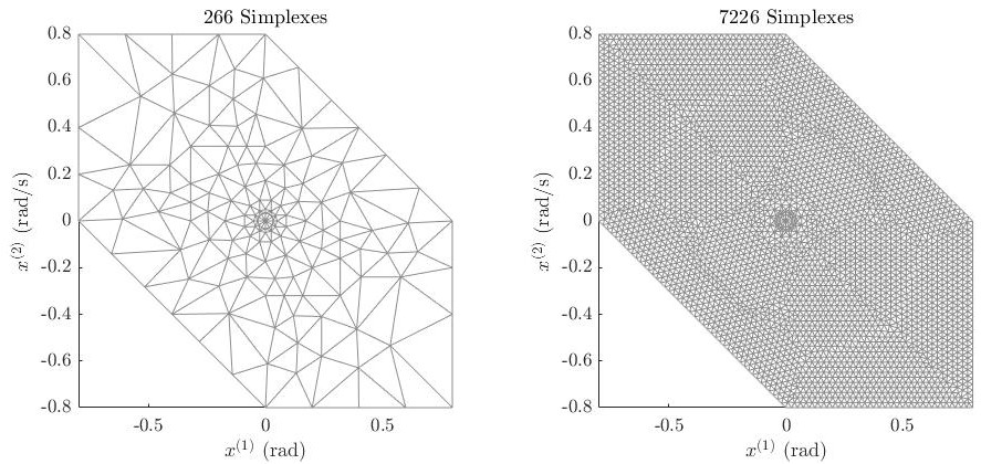
Figure 1: Two different unifrom triangulations for the region, $\Omega$, about the origin for dynamical system, $\mathcal{G}$.

IV-A Pendulum

Consider $\mathcal{G}$ with $k(\mathbf{x})=1$; this is a classic pendulum. Previous work, [14], could not be used to bound the $\mathcal{L}_{2}$-gain of an pendulum because $k(\mathbf{x})$ is a linear term and therefore did not have the property, $\left\lVert g(\mathbf{x})^{\top}g(\mathbf{x})\right\rVert_{\infty}=0$ at $\mathbf{x}=0$. However, the new convex optimization removes this requirement, so Problem 12 can now be used on the wide range of systems that have linear control terms.

From Equation 18, the $\mathcal{L}_{2}$-gain of $\mathcal{G}$ satisfies $\gamma\leq 1$. Figure 2 shows the result of optimizing Problem 12 for an increasing number of $n$-simplexes, as well as the time taken to complete this convex optimization. The $\mathcal{L}_{2}$-gain bound decreases as the triangulation becomes more refined, and reaches its lowest at $\gamma\leq 1.26$ when optimizing Problem 12 for 7226 $n$-simplexes. Applying Theorem 5 with Initialization 4 from [14], the small-signal property for this system to remain in $\Omega$ was found to be $||u(t)||_{\infty}\leq 0.077.$

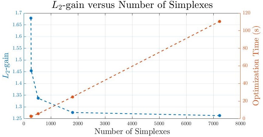
Figure 2: The $\mathcal{L}_{2}$-gain of a classic pendulum was solved with an increasing number of simplexes – resulting in the best estimate of $\gamma\leq 1.26.$

IV-B Pendulum with Control Affine Input

The variation $k(\mathbf{x})=x_{2}$ is considered here to compare with previous work [14]. From Equation 18, $\gamma\leq\max\{x_{2}^{2}|x_{2}\in\Omega\}$. For the given $\Omega,$ $\gamma\leq 0.64.$ Previous work developed a non-convex optimization problem and solved it using ICO, which only guarantees convergence to a local minima, creating more conservative bounds than Problem 12. In [14], the gain bound was found to be $\gamma\leq 3.85.$ In comparison, the best $\mathcal{L}_{2}$ gain bound found using the techniques developed in this paper was $\gamma\leq 0.76$ with the small signal property, $||u(t)||_{\infty}\leq 0.2554.$ Figure 3 shows the optimal gain bound found when solving Problem 12 over different numbers of $n$-simplexes. Even at the lowest number of $n$-simplexes, the gain bound still outperforms [14] by finding a bound of $\gamma\leq 1.11.$

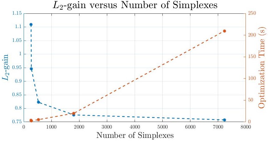
Figure 3: A pendulum with linear control affine input was analyzed for increasing numbers of simplexes over $\Omega.$ The $\mathcal{L}_{2}$ gain bound was found to be $\gamma\leq 0.76.$

V DISCUSSION

This work developed a convex optimization problem to determine the $\mathcal{L}_{2}$-gain of a dynamical system for a triangulated region about the origin. By reformulating the HJI as an LMI and developing novel LMI error bounds for a triangulation, the system’s gain can be bounded more tightly than a previous method, [14]. A limitation of this current method is that it can only be applied to bounded regions of the system’s state space, so future work should consider methods to expand this technique to the entire state space.

References

- [1] G. Zames, “On the input-output stability of time-varying nonlinear feedback systems part one: Conditions derived using concepts of loop gain, conicity, and positivity,” IEEE transactions on automatic control, vol. 11, no. 2, pp. 228–238, 1966.
- [2] K. Zhou and J. C. Doyle, Essentials of robust control. Prentice hall Upper Saddle River, NJ, 1998, vol. 104.
- [3] A. J. Van Der Schaft, “-gain analysis of nonlinear systems and nonlinear state feedback H∞ control,” IEEE Transactions on Automatic Control, vol. 37, no. 6, pp. 770–784, 1992.
- [4] H. Zhang and P. M. Dower, “Performance bounds for nonlinear systems with a nonlinear -gain property,” International Journal of Control, vol. 85, no. 9, pp. 1293–1312, 2012.
- [5] D. Hill and P. Moylan, “The stability of nonlinear dissipative systems,” IEEE transactions on automatic control, vol. 21, no. 5, pp. 708–711, 1976.
- [6] B. Brogliato, R. Lozano, B. Maschke, and O. Egeland, Dissipative Systems Analysis and Control: Theory and Applications, 2nd ed. London, UK: Springer Verlag, 2007.
- [7] S. Ratschan and Z. She, “Providing a basin of attraction to a target region of polynomial systems by computation of Lyapunov-like functions,” SIAM Journal on Control and Optimization, vol. 48, no. 7, pp. 4377–4394, 2010.
- [8] Z. Jarvis-Wloszek, R. Feeley, W. Tan, K. Sun, and A. Packard, “Some controls applications of sum of squares programming,” in 42nd IEEE international conference on decision and control (IEEE Cat. No. 03CH37475), vol. 5. IEEE, 2003, pp. 4676–4681.
- [9] H. Dai, B. Landry, L. Yang, M. Pavone, and R. Tedrake, “Lyapunov-stable neural-network control,” arXiv preprint arXiv:2109.14152, 2021.
- [10] Y.-C. Chang, N. Roohi, and S. Gao, “Neural Lyapunov control,” Advances in neural information processing systems, vol. 32, 2019.
- [11] P. Julian, J. Guivant, and A. Desages, “A parametrization of piecewise linear Lyapunov functions via linear programming,” International Journal of Control, vol. 72, no. 7-8, pp. 702–715, 1999.
- [12] P. Giesl and S. Hafstein, “Construction of Lyapunov functions for nonlinear planar systems by linear programming,” Journal of Mathematical Analysis and Applications, vol. 388, no. 1, pp. 463–479, 2012.
- [13] P. A. Giesl and S. F. Hafstein, “Revised CPA method to compute Lyapunov functions for nonlinear systems,” Journal of Mathematical Analysis and Applications, vol. 410, no. 1, pp. 292–306, 2014.
- [14] R. Lavaei and L. J. Bridgeman, “Iterative, small-signal stability analysis of nonlinear constrained systems,” arXiv preprint arXiv:2309.00517, 2023.
- [15] P. Fitzpatrick, Advanced calculus. American Mathematical Soc., 2009, vol. 5.
- [16] H. Khalil, Nonlinear Systems. Pearson Edu, Prentice Hall, 2002.
- [17] S. P. Boyd and L. Vandenberghe, Convex optimization. Cambridge university press, 2004.
- [18] R. J. Caverly and J. R. Forbes, “LMI properties and applications in systems, stability, and control theory,” arXiv preprint arXiv:1903.08599, 2019.
- [19] R. Lavaei and L. J. Bridgeman, “Systematic, lyapunov-based, safe and stabilizing controller synthesis for constrained nonlinear systems,” IEEE Transactions on Automatic Control, pp. 1–12, 2023.