A Schiffer-type problem for annuli
with applications to stationary planar Euler flows

Abstract.

If on a smooth bounded domain $\Omega\subset\mathbb{R}^{2}$ there is a nonconstant Neumann eigenfunction $u$ that is locally constant on the boundary, must $\Omega$ be a disk or an annulus? This question can be understood as a weaker analog of the well known Schiffer conjecture, in that the function $u$ is allowed to take a different constant value on each connected component of $\partial\Omega$ yet many of the known rigidity properties of the original problem are essentially preserved. Our main result provides a negative answer by constructing a family of nontrivial doubly connected domains $\Omega$ with the above property. As a consequence, a certain linear combination of the indicator functions of the domains $\Omega$ and of the bounded component of the complement $\mathbb{R}^{2}\backslash\overline{\Omega}$ fails to have the Pompeiu property. Furthermore, our construction implies the existence of continuous, compactly supported stationary weak solutions to the 2D incompressible Euler equations which are not locally radial.

1. Introduction

One of the most intriguing problems in spectral geometry is the so-called Schiffer conjecture, that dates back to the 1950s. In his 1982 list of open problems, S.T. Yau stated it (in the case $n=2$) as follows [29, Problem 80]:

Conjecture.

If a nonconstant Neumann eigenfunction $u$ of the Laplacian on a smooth bounded domain $\Omega\subset\mathbb{R}^{n}$ is constant on the boundary $\partial\Omega$, then $u$ is radially symmetric and $\Omega$ is a ball.

This overdetermined problem is closely related to the Pompeiu problem [22], an open question in integral geometry with many applications in remote sensing, image recovery and tomography [2, 28, 25]. The Pompeiu problem can be stated as the following inverse problem: Given a bounded domain $\Omega\subset\mathbb{R}^{n}$, is it possible to recover any continuous function $f$ on $\mathbb{R}^{n}$ from knowledge of its integral over all the domains that are the image of $\Omega$ under a rigid motion? If this is the case, so that the only $f\in C(\mathbb{R}^{n})$ satisfying

(1.1) $$\int_{{\mathcal{R}}(\Omega)}f(x)\,dx=0\,,$$

for any rigid motion ${\mathcal{R}}$ is $f\equiv 0$, the domain $\Omega$ is said to have the Pompeiu property. Squares, polygons, convex domains with a corner, and ellipses have the Pompeiu property, and Chakalov was apparently the first to point out that balls fail to have the Pompeiu property [6, 4, 30]. In 1976, Williams proved [27] that a smooth bounded domain with boundary homeomorphic to a sphere fails to have the Pompeiu property if and only if it supports a nontrivial Neumann eigenfunction which is constant on $\partial\Omega$. Therefore, the Schiffer conjecture is equivalent to saying that balls are the unique smooth bounded domains with boundary homeomorphic to a sphere without the Pompeiu property.

Although the Schiffer conjecture is famously open, some partial results are available. It is known that $\Omega$ must indeed be a ball under one of the following additional hypotheses:

1. There exists an infinite sequence of orthogonal Neumann eigenfunctions that are constant on $\partial\Omega$, which is connected [2, 3].

2. The third order interior normal derivative of $u$ is constant on $\partial\Omega$, which is connected [20].

In dimension 2, some further results are available, and the conjecture has been shown to be true in some other special cases:

1. When $\Omega$ is simply connected and $u$ has no saddle points in the interior of $\Omega$ [28].

2. If $\Omega$ is simply connected and the eigenvalue $\mu$ is among the seven lowest Neumann eigenvalues of the domain (twelve, if one assumes that $\Omega$ is convex) [1, 9].

3. If the fourth or fifth order interior normal derivative of $u$ is constant on $\partial\Omega$ [17].

It is also known that the boundary of any reasonably smooth domain $\Omega\subset\mathbb{R}^{n}$ with the property stated in the Schiffer conjecture must be analytic as a consequence of a result of Kinderlehrer and Nirenberg [19] on the regularity of free boundaries.

If one considers domains with disconnected boundary, it is natural to wonder what happens if one relaxes the hypotheses in the Schiffer conjecture by allowing the eigenfunction to be locally constant on the boundary, that is, constant on each connected component of $\partial\Omega$. Of course, the radial Neumann eigenfunctions of a ball or an annulus are locally constant on the boundary, so the natural question in this case is whether $\Omega$ must be necessarily a ball or an annulus.

We emphasize that this question shares many features with the Schiffer conjecture. First, essentially the same arguments show that $\partial\Omega$ must be analytic. Moreover, in the spirit of [2, 3], we show that if there exists an infinite sequence of orthogonal eigenfunctions that are locally constant on the boundary of $\Omega\subset\mathbb{R}^{2}$, then $\Omega$ must be a disk or an annulus. Furthermore, we prove that if the Neumann eigenvalue is sufficiently low, $\Omega$ must be a disk or an annulus, which is a result along the lines of [1, 9]. Precise statements and proofs of these rigidity results can be found in Section 6.

Our objective in this paper is to give a negative answer to this question. Indeed, we can prove the following:

Theorem 1.1.

There exist parametric families of doubly connected bounded domains $\Omega\subset\mathbb{R}^{2}$ such that the Neumann eigenvalue problem

$$\Delta u+\mu u=0\quad in\ \Omega\,,\qquad\partial_{\nu}u=0\quad on\ \partial\Omega\,,$$

admits, for some $\mu\in\mathbb{R}$, a non-radial eigenfunction that is locally constant on the boundary (i.e., $\nabla u\equiv 0$ on $\partial\Omega$). More precisely, for any large enough integer $l$ and for all $s$ in a small neighborhood of $0$, the family of domains $\Omega\equiv\Omega_{l,s}$ are given in polar coordinates by

(1.2) $$\Omega:=\big{\{}(r,\theta)\in\mathbb{R}^{+}\times\mathbb{T}:a_{l}+s\,b_{l,s}(\theta)<r<1+s\,B_{l,s}(\theta)\big{\}}\,,$$

where $b_{l,s},B_{l,s}$ are analytic functions of the form

$$b_{l,s}(\theta)=\alpha_{l}\cos l\theta+o(1)\,,\qquad B_{l,s}(\theta)=\beta_{l}\cos l\theta+o(1)\,,$$

$a_{l}\in(0,1)$, $\alpha_{l}$ and $\beta_{l}$ are nonzero constants, and where the $o(1)$ terms tend to $0$ as $s\to 0$.

We refer to Theorem 4.5 in the main text for a more precise statement.

In view of the connection between the Schiffer conjecture and the Pompeiu problem, it stands to reason that the domains of the main theorem should be connected with an integral identity somewhat reminiscent of the Pompeiu property. Specifically, one can prove the following corollary of our main result, which is an analog of the identity (1.1) in which one replaces the indicator function $\mathbbm{1}_{\Omega}$ implicit in the integral by a linear combination of indicator functions:

Corollary 1.2.

Let  $\Omega$ be a domain as in Theorem 1.1 and let $\Omega^{\prime}:=\{r<a_{l}+s\,b_{l,s}(\theta)\}$ denote the bounded component of $\mathbb{R}^{2}\backslash\overline{\Omega}$. Then there exists a positive constant $c$ and a nonzero function $f\in C^{\infty}(\mathbb{R}^{2})$ such that

$$\int_{{\mathcal{R}}(\Omega)}f\,dx-c\int_{{\mathcal{R}}(\Omega^{\prime})}f\,dx=0\,,$$

for any rigid motion ${\mathcal{R}}$.

Non-radial compactly supported solutions to the 2D Euler equations

Theorem 1.1 implies the existence of a special type of stationary 2D Euler flows, which was the original motivation of our work. Let us now describe this connection in detail.

It is well known that if a scalar function $w$ satisfies a semilinear equation of the form

(1.3) $$\Delta w+g(w)=0\quad\textup{in }\mathbb{R}^{2}\,,$$

for some function $g$, then the velocity field and pressure function given by

$$v:=\left(\frac{\partial w}{\partial x_{2}},-\frac{\partial w}{\partial x_{1}}\right)\,,\qquad p:=-\frac{1}{2}|\nabla w|^{2}-\int_{0}^{w}g(s)\,ds\,,$$

define a stationary solution to the Euler equations:

(1.4) $$v\cdot\nabla v+\nabla p=0\quad\textup{ and }\quad\operatorname{div}v=0\quad\textup{ in }\mathbb{R}^{2}\,.$$

Any function $w$ that is radial and compactly supported gives rise to a compactly supported stationary Euler flow in two dimensions, even if it does not solve a semilinear elliptic equation as above. The stationary solutions that are obtained by patching together radial solutions with disjoint supports are referred to as locally radial. For a detailed bibliography on the rigidity and flexibility properties of stationary Euler flows in two dimensions and their applications, we refer to the recent papers [13, 14].

Compactly supported stationary Euler flows in two dimensions that are not locally radial were constructed just very recently [13]. They are of vortex patch type and the velocity field is continuous but not differentiable. The proof of this result is hard: it involves several clever observations and a Nash–Moser iteration scheme. Furthermore, as emphasized in [13], these solutions cannot be obtained using an equation of the form (1.3). On the other hand, the existence of non-radial stationary planar Euler flows is constrained by several recent rigidity results [15, 14, 24]. We emphasize that the existence of $C^{1}$ compactly supported solutions of (1.4) which are not locally radial is not yet known (if the support condition is relaxed to having finite energy, the existence of smooth non-radial solutions follows directly from [21]).

In this context, one can readily use Theorem 1.1 to construct families of continuous compactly supported stationary Euler flows on the plane that are not locally radial. These solutions, which are not of patch type, are analytic in $\Omega$ but fail to be differentiable on the boundary of their support.

Theorem 1.3.

Let $\Omega$ be a domain as in Theorem 1.1. Then there exists a continuous, compactly supported stationary solution $(v,p)$ to the incompressible Euler equations on the plane such that $\operatorname{supp}v=\overline{\Omega}$. Furthermore, $(v,p)$ is analytic in $\Omega$.

We believe that the same strategy we use in this paper can be generalized for some nonlinear functions $g$ in Equation (1.3), which can be engineered to produce interesting nontrivial solutions to the incompressible Euler equations. We will explore this direction in the future.

Strategy of the proof of Theorem 1.1

Since any radial Neumann eigenfunction of an annulus is locally constant on the boundary, the basic idea of the proof of Theorem 1.1 is to construct $\Omega$ by bifurcating from a 1-parameter family of annuli. Specifically, we have chosen to bifurcate from the second nontrivial radial eigenfunction of the annuli. The reason for not choosing the first is that, in such case, the maximum and the minimum of the eigenfunction are attained at the boundary, and this is the setting in which the symmetry result of [23] holds. Hence, we do not expect that nonradial solutions can bifurcate from the first nontrivial radial eigenfunction of annuli.

To implement the bifurcation argument, the naive approach would be to carry out the analysis using one-variable functions $b(\theta),B(\theta)$ defined on the circle $\mathbb{T}$ to parametrize the boundary, as suggested by the expression (1.2). However, this leads to linearized operators that involve a serious loss of derivatives, which we do not know how to compensate using a Nash–Moser iteration scheme.

Instead, the strategy we follow is influenced by a very clever recent paper of Fall, Minlend and Weth [10]. Our main unknown is a two-variable function $v(r,\theta)$ defined on the annulus $\{\frac{1}{2}<r<1\}$. To control the regularity of $v$, we use anisotropic Hölder spaces, as the functions that arise naturally are one derivative smoother in $r$ than they are in $\theta$. Fall, Minlend and Weth introduced this strategy to construct the first examples of domains in the sphere that admit a Neumann eigenfunction which is constant on the boundary and whose boundary has nonconstant principal curvatures, thereby disproving a conjecture of Souam [26]. We refer to [10] for results on analogs of the Schiffer conjecture on manifolds.

In this functional setting we need to impose symmetry with respect to the group of isometries of an $l$-sided regular polygon. The key ingredient required to make the bifurcation argument work is a result about the crossing on certain Dirichlet and Neumann eigenvalues for annuli of certain radii, which takes place for $l\geqslant 4$. For technical reasons, we also have to exclude resonances with other Dirichlet eigenvalues. Once this is established, and using the functional framework described above, the proof of Theorem 1.1 follows from the Crandall–Rabinowitz theorem.

A considerable part of our paper is devoted to showing that the corresponding transversality condition holds. The proof is based on a delicate asymptotic analysis of Dirichlet and Neumann eigenfunctions on annuli in presence of a large parameter (namely, the angular mode of certain eigenfunction) and a small one (namely, the thickness of the annulus). What makes the analysis rather subtle is that these parameters are not independent, but related by the requirement that a certain pair of eigenvalues must coincide. This is the reason why we need to take a large integer $l$ in Theorem 1.1. However, this transversality condition can be numerically verified for specific values of $l$ with the help of Mathematica, so in Appendix A we show that this condition holds for $l=4$. This allows us to ensure that the conclusions of Theorem 1.1 also hold in the case $l=4$.

Organization of the paper

In Section 2 we prove the asymptotic estimates for the Dirichlet and Neumann eigenfunctions on annuli that are needed to establish eigenvalue crossing, non-resonance and transversality conditions. As discussed above, these will play a key role in the bifurcation argument later on. In Section 3 we reformulate the eigenvalue problem for a deformed annulus in terms of functions defined on a fixed domain and introduce the functional setting that we use. The proof of Theorem 1.1 is presented in Section 4. The applications to an analog of the Pompeiu problem and to the construction of non-radial stationary Euler flows on the plane are developed in Section 5. For completeness, in Section 6 we establish two rigidity results for the problem considered in this paper. We first show how existing arguments on the Schiffer problem prove that if a domain has infinitely many Neumann eigenfunctions that are locally constant on the boundary, then such domain is either a disk or an annulus. Then, we show that if the Neumann eigenvalue $\mu$ is sufficiently low, then $\Omega$ must be as well either a disk or an annulus. The paper is concluded with an Appendix where, using some elementary numerical computations, we show that the transversality condition holds for $l=4$.

2. The Dirichlet and Neumann spectrum of an annulus

In this section we shall establish the auxiliary results about Dirichlet and Neumann eigenvalues of annular domains that we will need in the proof of Theorem 1.1.

In view of the scaling properties of the Laplacian, it suffices to consider annuli with fixed outer radius. In polar coordinates $(r,\theta)\in\mathbb{R}^{+}\times\mathbb{T}$, let us therefore consider the annular domain

$$\Omega_{a}:=\{(r,\theta)\in(a,1)\times\mathbb{T}\}\,,$$

where $a\in(0,1)$ and $\mathbb{T}:=\mathbb{R}/2\pi\mathbb{Z}$. It is well known that an orthogonal basis of Neumann eigenfunctions in $\Omega_{a}$ is given by

$$\{\psi_{0,n}(r),\psi_{l,n}(r)\cos l\theta,\psi_{l,n}(r)\sin l\theta\}_{l=1,n=0}^{\infty}\,.$$

Here $\{\psi_{l,n}\}_{n=0}^{\infty}$ is an orthonormal basis of eigenfunctions of the associated radial operator. To put it differently, these functions (whose dependence on $a$ we omit notationally) satisfy the ODE

($${\rm N}_{a}^{l} \psi_{l,n}^{\prime\prime}+\frac{\psi_{l,n}^{\prime}}{r}-\frac{l^{2}\psi_{l,n}}{r^{2}}+\mu_{l,n}(a)\,\psi_{l,n}=0\quad\text{in }(a,1)\,,\qquad\psi_{l,n}^{\prime}(a)=\psi_{l,n}^{\prime}(1)=0\,,$$)

for some nonnegative constants

$$\mu_{l,0}(a)<\mu_{l,1}(a)<\mu_{l,2}(a)<\cdots<\mu_{l,n}(a)<\,\cdots$$

tending to infinity as $n\to\infty$. We will omit the dependence on $a$ when no confusion may arise.

The Neumann spectrum of the annulus $\Omega_{a}$ is then $\{\mu_{l,n}\}_{l,n=0}^{\infty}$. Let us record here the following immediate properties of these eigenvalues:

$$\mu_{0,0}=0\quad\textup{ and }\quad\mu_{l,n}<\mu_{l^{\prime},n}\ \mbox{ if }l<l^{\prime}\,.$$

Moreover, note that the eigenvalues of $\Omega_{a}$ may have multiplicity larger than 1 if $\mu_{l,n}=\mu_{l^{\prime},n^{\prime}}$ for some $(l,n)\neq(l^{\prime},n^{\prime})$. Here, when we talk about mulitiplicity we do not consider rotations of the same eigenfunction (that is, we only take $\cos(l\theta)$, for instance).

Likewise, an orthogonal basis of Dirichlet eigenfunctions of the annulus $\Omega_{a}$ is

$$\{\varphi_{0,n}(r),\varphi_{l,n}(r)\cos l\theta,\varphi_{l,n}(r)\sin l\theta\}_{l=1,n=0}^{\infty}\,,$$

where now the radial eigenfunctions satisfy the ODE

($${\rm D}_{a}^{l} \varphi_{l,n}^{\prime\prime}+\frac{\varphi_{l,n}^{\prime}}{r}-\frac{l^{2}\varphi_{l,n}}{r^{2}}+\lambda_{l,n}(a)\,\varphi_{l,n}=0\quad\text{in }(a,1)\,,\qquad\varphi_{l,n}(a)=\varphi_{l,n}(1)=0\,,$$)

for some positive constants

$$\lambda_{l,0}(a)<\lambda_{l,1}(a)<\lambda_{l,2}(a)<\cdots<\lambda_{l,n}(a)<\,\cdots$$

tending to infinity as $n\to\infty$. The Dirichlet spectrum of $\Omega_{a}$ is therefore $\{\lambda_{l,n}\}_{l,n=0}^{\infty}$. Again, we have

$$\lambda_{l,n}<\lambda_{l^{\prime},n}\ \mbox{ if }l<l^{\prime}\,.$$

Observe also that, thanks to the min-max characterization of the eigenvalues, the Neumann and Dirichlet eigenvalues are ordered, i.e.

$$\mu_{l,n}<\lambda_{l,n}\,.$$

In the following elementary lemma we show a property relating radial Neumann eigenvalues with Dirichlet ones. This is a variation on the fact that the derivative of a (nonconstant) radial Neumann eigenfunction is a Dirichlet eigenfunction.

Lemma 2.1.

For any $n\geqslant 1$, $\mu_{0,n}=\lambda_{1,n-1}.$

Proof.

Recall that $\psi_{0,n}$ is a solution to

$$\psi_{0,n}^{\prime\prime}+\frac{\psi_{0,n}^{\prime}}{r}+\mu_{0,n}\,\psi_{0,n}=0\quad\text{in }(a,1)\,,\qquad\psi_{0,n}^{\prime}(a)=\psi_{0,n}^{\prime}(1)=0\,.$$

Moreover, $\psi_{0,n}$ has exactly $n$ changes of sign in the interval $(a,1)$. As a consequence, $\phi=\psi_{0,n}^{\prime}$ changes sign $n-1$ times. Differentiating the equation above, we obtain that $\phi$ solves

$$\phi^{\prime\prime}+\frac{\phi^{\prime}}{r}-\frac{\phi}{r^{2}}+\mu_{0,n}\,\phi=0\quad\text{in }(a,1)\,,\qquad\phi(a)=\phi(1)=0\,.$$

Since the solution space is one-dimensional, $\phi=\varphi_{1,n-1}$ (possibly up to a nonzero multiplicative constant), so the lemma is proved. ∎

Next we show that there exist annuli where the third radial Neumann eigenvalue and the first $l$-mode Dirichlet eigenvalue coincide, and where certain non-resonance conditions are satisfied. This technical result is the first key ingredient in the bifurcation argument that the proof of Theorem 1.1 hinges on.

Proposition 2.2.

For any integer $l\geqslant 4$, there exists some constant $a_{l}\in(0,1)$ such that

(2.1) $$\mu_{0,2}(a_{l})=\lambda_{l,0}(a_{l})\,.$$

Moreover, the following non-resonance condition holds:

(NR) $$\lambda_{l,0}(a_{l})\neq\lambda_{ml,n}(a_{l})\quad\textup{ for all }\quad(m,n)\neq(1,0).$$

Proof.

We set $h:=\tfrac{1-a}{\pi}$ and $r=:1-hx$. Suppose now that $h\ll 1$, so $a$ is very close to 1. By the variational characterization of $\mu_{0,2}$, we get

(2.2) $$\mu_{0,2}(a) =\inf_{\dim V=3}\,\max_{\psi\in V\setminus\{0\}}\frac{\displaystyle\int_{0}^{\pi}\psi^{\prime}(x)^{2}(1-hx)\,dx}{h^{2}\displaystyle\int_{0}^{\pi}\psi(x)^{2}(1-hx)\,dx}$$

$$=\big{[}h^{-2}+O(h^{-1})\big{]}\inf_{\dim V=3}\,\max_{\psi\in V\setminus\{0\}}\frac{\displaystyle\int_{0}^{\pi}\psi^{\prime}(x)^{2}\,dx}{\displaystyle\int_{0}^{\pi}\psi(x)^{2}\,dx}=4h^{-2}+O(h^{-1})\,.$$

Here, $V$ ranges over the set of 3-dimensional subspaces of $H^{1}((0,\pi))$.

Likewise, in the case of the first $l$-mode Dirichlet eigenvalue, we have

(2.3) $$\lambda_{l,0}(a) =\inf_{\varphi\in H_{0}^{1}((0,\pi))\setminus\{0\}}\,\frac{\displaystyle h^{-2}\int_{0}^{\pi}\psi^{\prime}(x)^{2}(1-hx)\,dx+l^{2}\int_{0}^{\pi}\frac{\psi(x)^{2}}{(1-hx)}\,dx}{\displaystyle\int_{0}^{\pi}\psi(x)^{2}(1-hx)\,dx}$$

$$=h^{-2}\left[\inf_{\varphi\in H_{0}^{1}(0,\pi)\setminus\{0\}}\,\frac{\int_{0}^{\pi}\psi^{\prime}(x)^{2}\,dx}{\int_{0}^{\pi}\psi(x)^{2}\,dx}+O(h)\right]+l^{2}(1+O(h))=\big{(}1+(hl)^{2}\big{)}\big{[}h^{-2}+O(h^{-1})\big{]}\,.$$

In particular, we conclude from these expressions for $\mu_{0,2}$ and $\lambda_{l,0}$ that

(2.4) $$\mu_{0,2}(a)>\lambda_{l,0}(a)$$

whenever $a$ is close enough to $1$.

We now show the converse inequality for $a$ small. In order to do that, recall that, by Lemma 2.1, $\mu_{0,2}(a)=\lambda_{1,1}(a)$. We now claim that for any $l\geqslant 1$, $k\geqslant 0$,

(2.5) $$\lambda_{l,k}(a)\to\lambda_{l,k}^{0}\,,\quad\textup{ as }a\to 0\,,$$

where we have set

$$\lambda_{l,k}^{0}:=\inf_{\dim V=k}\,\max_{\varphi\in V\setminus\{0\}}\frac{\displaystyle\int_{0}^{1}\Big{(}\varphi^{\prime}(r)^{2}+l^{2}\frac{\varphi(r)^{2}}{r^{2}}\Big{)}\,r\,dr}{\displaystyle\int_{0}^{1}\varphi(r)^{2}\,r\,dr}\,.$$

Here, $V$ ranges over the set of $k$-dimensional subspaces of $\mathcal{H}_{0}\subset\mathcal{H}$, where

$$\mathcal{H}:=\Big{\{}\varphi:(0,1)\to\mathbb{R}:\int_{0}^{1}\Big{(}\varphi^{\prime}(r)^{2}+\frac{\varphi(r)^{2}}{r^{2}}\Big{)}\,r\,dr<+\infty\ \Big{\}}\quad\textup{ and }\quad\mathcal{H}_{0}:=\big{\{}\varphi\in\mathcal{H}:\ \varphi(1)=0\big{\}}\,.$$

These spaces are equipped with the natural norm

$$\|\varphi\|_{\mathcal{H}}^{2}:=\int_{0}^{1}\left(\varphi^{\prime}(r)^{2}+\frac{\varphi(r)^{2}}{r^{2}}\right)\,r\,dr\,.$$

Note that the functions in $\mathcal{H}$ are continuous in $[0,1]$ and vanish at $0$, see e.g. [5, Proposition 3.1].

In other words, (2.5) simply asserts that the Dirichlet eigenvalues of the annulus $\Omega_{a}$ converge, as $a\to 0$, to the Dirichlet eigenvalues of the unit disk. This is well known, but we give a short self-contained proof for the convenience of the reader.

First, observe that $\lambda_{l,k}(a)$ is decreasing in $a$, and it is always bigger than $\lambda_{l,k}^{0}$. As a consequence, it has a limit and

$$\lim_{a\to 0}\lambda_{l,k}(a)\geqslant\lambda_{l,k}^{0}\,.$$

To show the converse inequality, it suffices to prove that any function in $\mathcal{H}_{0}$ can be approximated by functions vanishing in a neighborhood of $0$. For this, let us choose a smooth cut-off function $\chi:[0,+\infty)\to[0,1]$ such that $\chi|_{[0,1]}=1$ and $\chi_{[2,+\infty)}=0$, and define $\chi_{\varepsilon}(r):=\chi(\frac{r}{\varepsilon})$ for $\varepsilon$ sufficiently small. We shall next show that, given any $\varphi\in\mathcal{H}$, $\chi_{\varepsilon}\varphi\to 0$ in $\mathcal{H}$ as $\varepsilon\to 0$. This obviously implies (2.5) since in this case $(1-\chi_{\varepsilon})\varphi\to\varphi$ in $\mathcal{H}$.

To show that $\chi_{\varepsilon}\varphi\to 0$ in $\mathcal{H}$, we first note that

$$\int_{0}^{1}\frac{\chi_{\varepsilon}(r)^{2}\varphi(r)^{2}}{r}\leqslant\int_{0}^{\varepsilon}\frac{\varphi(r)^{2}}{r}\to 0\,,\quad\textup{ as }\varepsilon\to 0\,.$$

Moreover, as $\varepsilon\to 0$,

$$\int_{0}^{1}\chi_{\varepsilon}(r)^{2}\varphi^{\prime}(r)^{2}r\,dr\leqslant\int_{0}^{\varepsilon}\varphi^{\prime}(r)^{2}r\,dr\to 0\,,$$

and

$$\int_{0}^{1}\chi_{\varepsilon}^{\prime}(r)^{2}\varphi(r)^{2}r\,dr\leqslant\frac{\|\chi^{\prime}\|_{L^{\infty}}^{2}}{\varepsilon^{2}}\int_{0}^{\varepsilon}\varphi(r)^{2}r\,dr\leqslant\frac{\|\chi^{\prime}\|_{L^{\infty}}^{2}}{\varepsilon}\int_{0}^{\varepsilon}\varphi(r)^{2}\,dr\leqslant\|\chi^{\prime}\|_{L^{\infty}}^{2}\|\varphi\|_{L^{\infty}([0,\varepsilon])}^{2}\to 0\,,$$

since $\varphi$ is continuous in $[0,1]$ and $\varphi(0)=0$. As $(\chi_{\varepsilon}\varphi)^{\prime}=\chi_{\varepsilon}^{\prime}\varphi+\chi_{\varepsilon}\varphi^{\prime}$, it follows that $\chi_{\varepsilon}\varphi\to 0$ in ${\mathcal{H}}$ and thus (2.5) follows.

We now compute the eigenvalues $\lambda_{1,1}^{0}$ and $\lambda_{l,0}^{0}$, which can be written explicitly in terms of Bessel zeros. More precisely, it is known that if $j_{m,k}$ is the $k$-th positive zero of the Bessel function of the first kind $J_{m}$, then

$$\lambda_{l,k}^{0}=j_{l,k+1}^{2}\,.$$

The numerical values of the zeros are well known, e.g.,

$$j_{1,2}=7.01559\dots$$

and

$$j_{1,1}=3.83171\dots\,,\quad j_{2,1}=5.13562\dots\,,\quad j_{3,1}=6.38016\dots\,,\quad j_{4,1}=7.58834\dots\,.$$

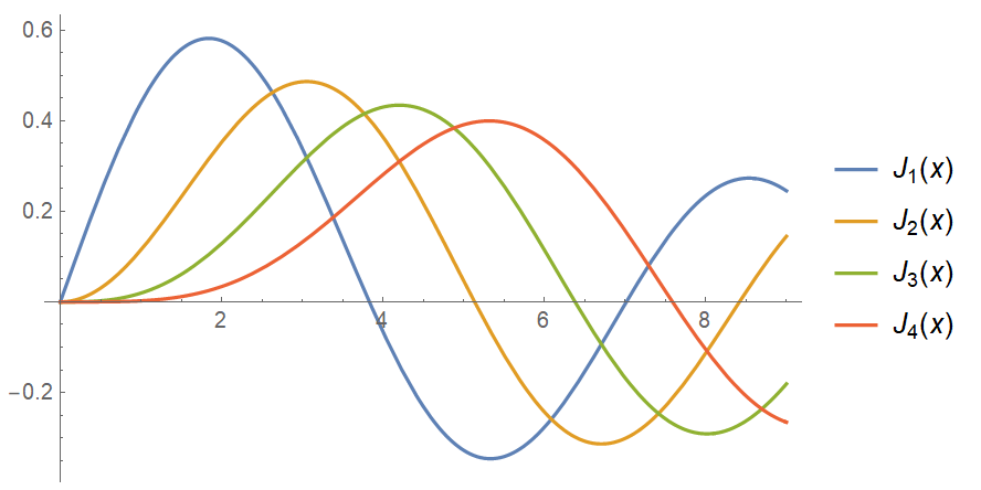
Figure 1. The first positive zero of $J_{l}$ is bigger than the second positive zero of $J_{1}$ if $l\geqslant 4$.

Therefore, $\lambda_{1,1}^{0}<\lambda_{l,0}^{0}$ for any $\l\geqslant 4$. By (2.5) we obtain that, for any integer $l\geqslant 4$ and for sufficiently small $a$, $\mu_{0,2}(a)<\lambda_{l,0}(a)$. This inequality, together with (2.4) and the continuous dependence of the eigenvalues on $a$ (see e.g. [16, Section II.7]), allows us to conclude the existence of $a_{l}\in(0,1)$ such that (2.1) holds.

We now turn our attention to (NR). In the rest of the proof, we fix $a:=a_{l}$, omitting the dependence on this variable for the ease of notation. First of all, by the strict monotonicity with respect to $l$ and $n$ of the Neumann and Dirichlet eigenvalues, it follows that

$$\lambda_{l,n}>\lambda_{l,0}\ \textup{ for all }n\geqslant 1\,,\qquad\lambda_{ml,n}\geqslant\lambda_{ml,0}>\lambda_{l,0}\ \textup{ for all }m\geqslant 2,\ n\geqslant 0\,.$$

Moreover,

$$\lambda_{0,0}<\lambda_{l,0}\,,\qquad\lambda_{0,n}\geqslant\lambda_{0,2}>\mu_{0,2}=\lambda_{l,0}\ \mbox{ if }n\geqslant 2\,.$$

Finally, by Lemma 2.1, $\mu_{0,2}=\lambda_{1,1}$, which is clearly bigger than $\lambda_{0,1}$. The proposition is then proved. ∎

Next proposition is devoted to prove an estimate which will imply the usual transversality condition in the Crandall–Rabinowitz theorem. We prove this estimate for any sufficiently large $l$, and refer to Appendix A for the direct verification of this condition in the case $l=4$ (the same strategy could be used for other specific values of $l$). In the statement, we denote by a prime the derivative of an eigenvalue with respect to the parameter $a$.

Proposition 2.3.

For any large enough integer $l$, the constant $a_{l}$ introduced in Proposition 2.2 is of the form

(2.6) $$a_{l}=1-\frac{\sqrt{3}\pi}{l}+O(l^{-2})\,.$$

Moreover, the following transversality condition holds:

(T) $$\mu_{0,2}^{\prime}(a_{l})\neq\lambda_{l,0}^{\prime}(a_{l})\,.$$

Proof.

The proof will be divided into four steps for the sake of clarity.

Step 1: Zeroth order estimates

In this first step we prove (2.6). First of all, observe that

(2.7) $$\lambda_{l,0}(a):=\inf_{\varphi\in H_{0}^{1}((a,1))\setminus\{0\}}\displaystyle\frac{\displaystyle\int_{a}^{1}\Big{(}\varphi^{\prime}(r)^{2}+\frac{l^{2}}{r^{2}}\varphi(r)^{2}\Big{)}\,r\,dr}{\displaystyle\int_{a}^{1}\varphi(r)^{2}r\,dr}\geqslant l^{2}\,,\quad\textup{ for all }a\in(0,1)\,.$$

This implies in particular that, for any sufficiently large integer $l$,

(2.8) $$\lambda_{l,0}(\tfrac{1}{2})>\mu_{0,2}(\tfrac{1}{2})\,.$$

As a consequence, we can take $a_{l}\in(\tfrac{1}{2},1)$ for sufficiently large $l$. As in the proof of Proposition 2.2, we define $h_{l}:=\tfrac{1-a_{l}}{\pi}$ and $r=:1-h_{l}x$. Then, we can estimate

$$\mu_{0,2}(a_{l}) =\inf_{\dim V=3}\,\max_{\psi\in V\setminus\{0\}}\frac{\displaystyle\int_{0}^{\pi}\psi^{\prime}(x)^{2}(1-h_{l}x)\,dx}{h_{l}^{2}\displaystyle\int_{0}^{\pi}\psi(x)^{2}(1-h_{l}x)\,dx} \leqslant\inf_{\dim V=3}\,\max_{\psi\in V\setminus\{0\}}\frac{2\displaystyle\int_{0}^{\pi}\psi^{\prime}(x)^{2}\,dx}{\displaystyle h_{l}^{2}\int_{0}^{\pi}\psi(x)^{2}\,dx}=8h_{l}^{-2}$$

which, together with (2.7), implies that $h_{l}=O(l^{-1})$ for large $l$. Note that in the inequality we have used that $a_{l}\in(\frac{1}{2},1)$, so $h_{l}\leqslant 2/\pi$. Hence, we can use the asymptotic formulas (2.2)-(2.3) to infer that

$$4+O(h_{l})=1+(h_{l}l)^{2}\,.$$

Thus, (2.6) holds.

Step 2: First order estimates and asymptotics for $a_{l}$

Our goal now is to obtain a more accurate asymptotic estimate for $a_{l}$ in terms of $l\gg 1$. To this end, let us introduce the differential operator

(2.9) $$T_{\eta,\varepsilon}:=\partial_{x}^{2}-\frac{\eta(1+\varepsilon)}{1-\eta(1+\varepsilon)x}\,\partial_{x}-\frac{3(1+\varepsilon)^{2}}{(1-\eta(1+\varepsilon)x)^{2}}\,.$$

Here $(\eta,\varepsilon)$ are real constants, which can be assumed to be suitably small (say, $|\eta|+|\epsilon|<\tfrac{1}{100}$). Note that for $\eta=\varepsilon=0$, the operator is simply $T_{0,0}=\partial_{x}^{2}-3$.

Let us respectively denote by $\Lambda_{n}(\eta,\varepsilon)$ and ${\nu}_{n}(\eta,\varepsilon)$ the Dirichlet and Neumann eigenvalues of the operator $T_{\eta,\varepsilon}$ on the interval $(0,\pi)$, where $n$ ranges over the nonnegative integers. It is standard (and easy to see) that all these eigenvalues have multiplicity 1, so it is well known [16, Section II.7] that the eigenvalues and their corresponding eigenfunctions (which we will respectively denote by $\Phi_{n}(\eta,\varepsilon)$ and $\Psi_{n}(\eta,\varepsilon)$) depend analytically on $(\eta,\varepsilon)$. Therefore, for all $n\geqslant 0$, we can assume that

($${\rm N}_{\eta,\varepsilon} T_{\eta,\varepsilon}\Psi_{n}+\nu_{n}(\eta,\varepsilon)\Psi_{n}=0\quad\textup{in }(0,\pi)\,,\qquad\Psi_{n}^{\prime}(0)=\Psi_{n}^{\prime}(\pi)=0\,,$$)

and

($${\rm D}_{\eta,\varepsilon} T_{\eta,\varepsilon}\Phi_{n}+\Lambda_{n}(\eta,\varepsilon)\Phi_{n}=0\quad\textup{in }(0,\pi)\,,\qquad\Phi_{n}(0)=\Phi_{n}(\pi)=0\,.$$)

Likewise, we introduce the operator

(2.10) $$\widetilde{T}_{\eta,\varepsilon}:=\partial_{x}^{2}-\frac{\eta(1+\varepsilon)}{1-\eta(1+\varepsilon)x}\,\partial_{x}\,,$$

and, for all nonnegative integer $n$, we denote by $\widetilde{\nu}_{n}(\eta,\varepsilon)$ and $\widetilde{\Lambda}_{n}(\eta,\varepsilon)$ the Neumann and Dirichlet eigenvalues in $(0,\pi)$ with corresponding eigenfunctions $\widetilde{\Psi}_{n}(\eta,\epsilon)$ and $\widetilde{\Phi}_{n}(\eta,\varepsilon)$ respectively. In other words,

($${\rm\widetilde{N}}_{\eta,\varepsilon} \widetilde{T}_{\eta,\varepsilon}\widetilde{\Psi}_{n}+\widetilde{\nu}_{n}(\eta,\varepsilon)\widetilde{\Psi}_{n}=0\quad\textup{in }(0,\pi)\,,\qquad\Psi_{n}^{\prime}(0)=\Psi_{n}^{\prime}(\pi)=0\,,$$)

and

($${\rm\widetilde{D}}_{\eta,\varepsilon} \widetilde{T}_{\eta,\varepsilon}\widetilde{\Phi}_{n}+\widetilde{\Lambda}_{n}(\eta,\varepsilon)\widetilde{\Phi}_{n}=0\quad\textup{in }(0,\pi)\,,\qquad\Phi_{n}(0)=\Phi_{n}(\pi)=0\,.$$)

We start with the proof of first order asymptotics for $\Lambda_{0}$ and $\widetilde{\nu}_{2}$:

Lemma 2.4.

For $|\eta|+|\varepsilon|\ll 1$,

$$\Lambda_{0}(\eta,\varepsilon) =4+3\pi\eta+6\varepsilon+O(\eta^{2}+\varepsilon^{2})\,,$$

$$\widetilde{\nu}_{2}(\eta,\varepsilon) =4+O(\eta^{2}+\varepsilon^{2})\,.$$

Proof.

Let us start with $\Lambda_{0}$. Noting that $\Phi_{00}(x):=\sin(x)$ is the first Dirichlet eigenfunction of $T_{0,0}=\partial_{x}^{2}-3$ on $(0,\pi)$ with eigenvalue $\Lambda_{00}:=4$, by the analytic dependence on the parameters, we can take an analytic two-parameter family of Dirichlet eigenfunctions of the form

$$\Phi_{0}(\eta,\varepsilon)(x):=\sum_{j,k\geqslant 0}\eta^{j}\varepsilon^{k}\,\Phi_{jk}(x)\,,\quad\textup{with}\quad\Phi_{jk}(0)=\Phi_{jk}(\pi)=0\,,\quad\textup{for all}\quad j,k\geqslant 0\,,$$

with corresponding eigenvalues

$$\Lambda_{0}(\eta,\varepsilon):=\sum_{j,k\geqslant 0}\eta^{j}\varepsilon^{k}\,\Lambda_{jk}\,.$$

Moreover, let us normalize $\Phi_{0}(\eta,\varepsilon)$ so that

$$\int_{0}^{\pi}\Phi_{0}(\varepsilon,\eta)(x)\sin(x)\,dx=\frac{\pi}{2}\,.$$

Since $\int_{0}^{\pi}\Phi_{00}(x)\sin(x)\,dx=\frac{\pi}{2}$, this implies

$$\int_{0}^{\pi}\Phi_{jk}(x)\sin(x)\,dx=0\quad\textup{for all}\quad(j,k)\neq(0,0)\,.$$

Let us now compute the first order terms in the expansion. Since

$$T_{\eta,\epsilon}=\partial_{x}^{2}+\big{(}\eta+\varepsilon\eta+\eta^{2}x-O(\varepsilon\eta^{2}+\eta^{3})\big{)}\,\partial_{x}\\ -\big{(}3+6\varepsilon+3\varepsilon^{2}+6\eta x+18\eta\varepsilon x+9\eta^{2}x^{2}+O(\eta^{2}\varepsilon+\varepsilon^{2}\eta+\eta^{3}+\varepsilon^{3})\big{)}\,,$$

defining $L:=\partial_{x}^{2}+\Lambda_{00}-3=\partial_{x}^{2}+1$, we get

$$0 =T_{\eta,\varepsilon}\Phi_{0}+\Lambda_{0}(\eta,\varepsilon)\Phi_{0}$$

$$=L\Phi_{00}+\varepsilon\Big{(}L\Phi_{01}+(\Lambda_{01}-6)\Phi_{00}\Big{)}+\eta\Big{(}L\Phi_{10}-\partial_{x}\Phi_{00}+(\Lambda_{10}-6x)\Phi_{00}\Big{)}+O(\eta^{2}+\varepsilon^{2})\quad\textup{in }(0,\pi)\,.$$

Also, as $\Lambda_{00}=4$ and $\Phi_{00}(x)=\sin(x)$, the zeroth order term vanishes, and we arrive at the equations

(2.11) $$L\Phi_{01}+(\Lambda_{01}-6)\Phi_{00} =0\,,$$

(2.12) $$L\Phi_{10}-\partial_{x}\Phi_{00}+(\Lambda_{10}-6x)\Phi_{00} =0\,.$$

Multiplying Equation (2.11) by $\Phi_{00}$ and integrating by parts, we easily find that $\Lambda_{01}=6$ and $\Phi_{01}\equiv 0$. Doing the same with (2.12), we get

$$\Lambda_{10}\,\frac{\pi}{2}=\Lambda_{10}\int_{0}^{\pi}\sin(x)^{2}\,dx=6\int_{0}^{\pi}x\sin(x)^{2}\,dx=\frac{3\pi^{2}}{2}\,,$$

so $\Lambda_{10}=3\pi$. We then conclude that

$$\Lambda_{0}(\eta,\varepsilon)=4+3\pi\eta+6\varepsilon+O(\eta^{2}+\varepsilon^{2})\,.$$

We now compute the first order expansion of $\widetilde{\nu}_{2}$. We start with the observation that $\widetilde{\Psi}_{00}(x):=\cos(2x)$ is the third Neumann eigenfunction of $\widetilde{T}_{0,0}=\partial_{x}^{2}$ in $(0,\pi)$, and that the corresponding eigenvalue is $\widetilde{\nu}_{00}:=4$. Arguing as above, we consider a convergent series expansion of the eigenvalue

$$\widetilde{\nu}_{2}(\eta,\varepsilon):=\sum_{j,k\geqslant 0}\eta^{j}\varepsilon^{k}\,\widetilde{\nu}_{jk}$$

and of the corresponding eigenfunction

$$\widetilde{\Psi}_{2}(\eta,\varepsilon)(x):=\sum_{j,k\geqslant 0}\eta^{j}\varepsilon^{k}\,\widetilde{\Psi}_{jk}(x)\,,\quad\textup{with}\quad\widetilde{\Psi}_{jk}^{\prime}(0)=\widetilde{\Psi}_{jk}^{\prime}(\pi)=0\,,\quad\textup{for all}\quad j,k\geqslant 0\,,$$

which we normalize so that

$$\int_{0}^{\pi}\widetilde{\Psi}_{2}(\eta,\varepsilon)(x)\,\cos(2x)dx=\frac{\pi}{2}=\int_{0}^{\pi}\widetilde{\Psi}_{00}(x)\,\cos(2x)dx\,.$$

Since

$$\widetilde{T}_{\eta,\varepsilon}=\partial_{x}^{2}-\big{(}\eta+\varepsilon\eta+\eta^{2}x+O(\varepsilon\eta^{2}+\eta^{3})\big{)}\,\partial_{x}\,,$$

just as in the case of $\Lambda_{0}$ we can write

$$0 =\widetilde{T}_{\eta,\varepsilon}\widetilde{\Psi}_{2}+\widetilde{\nu}_{2}(\eta,\varepsilon)\widetilde{\Psi}_{2}$$

$$=\widetilde{L}\widetilde{\Psi}_{00}+\varepsilon\Big{(}\widetilde{L}\widetilde{\Psi}_{01}+\widetilde{\nu}_{01}\widetilde{\Psi}_{00}\Big{)}+\eta\Big{(}\widetilde{L}\widetilde{\Psi}_{10}-\partial_{x}\widetilde{\Psi}_{00}+\widetilde{\nu}_{10}\widetilde{\Psi}_{00}\Big{)}+O(\eta^{2}+\varepsilon^{2})\quad\textup{in }(0,\pi)\,,$$

with $\widetilde{L}:=\partial_{x}^{2}+\widetilde{\nu}_{00}=\partial_{x}^{2}+4$. Arguing as we did in the analysis of $\Lambda_{0}$, multiplying the equations now by $\widetilde{\Psi}_{00}$ and integrating by parts, we infer that $\widetilde{\nu}_{01}=\widetilde{\nu}_{10}=0$, and thus we conclude that

$$\widetilde{\nu}_{2}(\eta,\varepsilon)=4+O(\eta^{2}+\varepsilon^{2})\,.$$

The lemma is then proved. ∎

Armed with this auxiliary estimate, we readily obtain the following second order formula for $a_{l}$:

Lemma 2.5.

There exists $\delta_{l}=O(l^{-1})$ such that

(2.13) $$\varepsilon_{l}=-\frac{\sqrt{3}\pi}{2l}\big{(}1+\delta_{l}\big{)}\,.$$

Proof.

With $\eta_{l}:=\tfrac{\sqrt{3}}{l}$, let us write $a_{l}=1-\eta_{l}(1+\varepsilon_{l})=:1-\pi h_{l}$. Using the change of variables $r=:1-h_{l}x$ as before, a direct calculation shows that the radial eigenvalue equation (${\rm N}_{a}^{l}$) is

$$T_{\eta_{l},\varepsilon_{l}}u+h_{l}^{2}\mu_{0,2}(a_{l})u=0\quad\textup{in }(0,\pi)\,,\qquad u^{\prime}(0)=u^{\prime}(\pi)=0\,,$$

which shows that

$$\mu_{0,2}(a_{l})=h_{l}^{-2}\,\widetilde{\nu}_{2}(\eta_{l},\varepsilon_{l})\,.$$

Similarly,

$$\lambda_{l,0}(a_{l})=h_{l}^{-2}\,\Lambda_{0}(\eta_{l},\varepsilon_{l})\,.$$

The condition $\lambda_{l,0}(a_{l})=\mu_{0,2}(a_{l})$ and the asymptotic formulas of Lemma 2.4 readily yield the desired expression for $\varepsilon_{l}$. ∎

Step 3: Second order estimates

In view of Lemma 2.5, in the operators $T_{\eta,\varepsilon}$ and $\widetilde{T}_{\eta,\varepsilon}$ it is natural to take $\varepsilon:=-\frac{\pi}{2}\eta(1+\delta)$ with $|\delta|\ll 1$. With some abuse of notation, we shall denote by

$$T_{\eta,\delta}:=\partial_{x}^{2}-\frac{\eta(1-\frac{\pi}{2}\eta(1+\delta))}{1-\eta(1-\frac{\pi}{2}\eta(1+\delta))x}\,\partial_{x}-\frac{3(1-\frac{\pi}{2}\eta(1+\delta))^{2}}{(1-\eta(1-\frac{\pi}{2}\eta(1+\delta))x)^{2}}$$

the resulting differential operator, and we shall use the notation $\nu_{n}(\eta,\delta)$, $\Lambda_{n}(\eta,\delta)$, $\Psi_{n}(\eta,\delta)$ and $\Phi_{n}(\eta,\delta)$ for its eigenvalues and eigenfunctions.

Likewise, we define

$$\widetilde{T}_{\eta,\delta}:=\partial_{x}^{2}-\frac{\eta(1-\frac{\pi}{2}\eta(1+\delta))}{1-\eta(1-\frac{\pi}{2}\eta(1+\delta))x}\,\partial_{x}\,,$$

and we use a similar notation for its eigenvalues and eigenfunctions: $\widetilde{\nu}_{n}(\eta,\delta)$, $\widetilde{\Lambda}_{n}(\eta,\delta)$, $\widetilde{\Psi}_{n}(\eta,\delta)$ and $\widetilde{\Phi}_{n}(\eta,\delta)$. Of course, the dependence on the new parameters $(\eta,\delta)$ is still analytic.

The second order asymptotic expansions that we need are the following:

Lemma 2.6.

For $|\eta|+|\delta|\ll 1$,

$$\Lambda_{0}(\eta,\delta) =4-3\pi\eta\delta-16\eta^{2}+O(|\eta|^{3}+|\delta|^{3})\,,$$

$$\nu_{1}(\eta,\delta) =4-3\pi\eta\delta+24\eta^{2}+O(|\eta|^{3}+|\delta|^{3})\,,$$

$$\widetilde{\nu}_{2}(\eta,\delta) =4+\tfrac{3}{4}\,\eta^{2}+O(|\eta|^{3}+|\delta|^{3})\,,$$

$$\widetilde{\Lambda}_{1}(\eta,\delta) =4+\tfrac{7}{2}\,\eta^{2}+O(|\eta|^{3}+|\delta|^{3})\,.$$

Proof.

We start with $\Lambda_{0}$. In the case $\eta=\delta=0$, it is clear that $\Phi_{00}(x):=\sin(x)$ is an eigenfunction of $T_{\eta,\delta}$ with eigenvalue $\Lambda_{00}:=4$. Hence, there exists an eigenfunction of the form

$$\Phi_{0}(\eta,\delta)(x):=\sum_{j,k\geqslant 0}\eta^{j}\delta^{k}\,\Phi_{jk}(x)\,,\quad\textup{with}\quad\Phi_{jk}(0)=\Phi_{jk}(\pi)=0\,,\quad\textup{for all}\quad j,k\geqslant 0\,,$$

with eigenvalue

$$\Lambda_{0}(\eta,\delta):=\sum_{j,k\geqslant 0}\eta^{j}\delta^{k}\,\Lambda_{jk}\,,$$

which we normalize as

$$\int_{0}^{\pi}\Phi_{0}(\eta,\delta)(x)\sin(x)\,dx=\frac{\pi}{2}=\int_{0}^{\pi}\Phi_{00}(x)\sin(x)\,dx\,,$$

to ensure that

$$\int_{0}^{\pi}\Phi_{jk}(x)\sin(x)\,dx=0\quad\textup{for all}\quad(j,k)\neq(0,0)\,.$$

Since

$$T_{\eta,\delta}=\partial_{x}^{2}-\big{(}\eta+(x-\tfrac{\pi}{2})\eta^{2}+O(\eta^{2}|\delta|+|\eta|^{3})\big{)}\,\partial_{x}\\ -\big{(}3-3(\pi-2x)\eta-3\pi\eta\delta+\frac{3}{4}(\pi^{2}-12\pi x+12x^{2})\eta^{2}+O(\eta^{2}|\delta|+|\eta|^{3})\big{)}\,,$$

arguing as in Lemma 2.4, the eigenvalue equation reads as

$$0 =T_{\eta,\delta}\Phi_{0}+\Lambda_{0}(\eta,\delta)\Phi_{0}$$

$$=L\Phi_{00}+\delta\Big{(}L\Phi_{01}+\Lambda_{01}\Phi_{00}\Big{)}+\delta^{2}\Big{(}L\Phi_{02}+\Lambda_{02}\Phi_{00}+\Lambda_{01}\Phi_{01}\Big{)}$$

$$\quad+\eta\Big{(}L\Phi_{10}-\partial_{x}\Phi_{00}+\big{(}\Lambda_{10}+3(\pi-2x)\big{)}\Phi_{00}\Big{)}$$

$$\quad+\eta^{2}\Big{(}L\Phi_{20}-\partial_{x}\Phi_{10}+(\tfrac{\pi}{2}-x)\partial_{x}\Phi_{00}+\big{(}\Lambda_{10}+3(\pi-2x)\big{)}\Phi_{10}+\big{(}\Lambda_{20}-\tfrac{3}{4}(\pi^{2}-12\pi x+12x^{2})\big{)}\Phi_{00}\Big{)}$$

$$\quad+\eta\delta\Big{(}L\Phi_{11}-\partial_{x}\Phi_{01}+\big{(}\Lambda_{10}+3(\pi-2x)\big{)}\Phi_{01}+\Lambda_{01}\Phi_{10}+(\Lambda_{11}+3\pi)\Phi_{00}\Big{)}+O\big{(}|\eta|^{3}+|\delta|^{3}\big{)}\quad\textup{in }(0,\pi)\,,$$

with $L:=\partial_{x}^{2}+1$. By the choice of $\Lambda_{00}$ and $\Phi_{00}$, the zeroth order term of the above expression cancels. Moreover, arguing as in Lemma 2.4, it is immediate to see that $\Lambda_{01}=\Lambda_{02}=0$ and that $\Phi_{01}\equiv\Phi_{02}\equiv 0$.

The first nontrivial equation we need to solve is

$$L\Phi_{10}-\partial_{x}\Phi_{00}+\big{(}\Lambda_{10}+3(\pi-2x)\big{)}\Phi_{00}=0\quad\textup{in }(0,\pi)\,.$$

Multiplying by $\Phi_{00}$ and integrating by parts, we get

$$\Lambda_{10}\,\frac{\pi}{2}=\Lambda_{10}\int_{0}^{\pi}\sin(x)^{2}\,dx=3\int_{0}^{\pi}(2x-\pi)\sin(x)^{2}\,dx=0\,,$$

so $\Lambda_{10}=0$. The equation can then be rewritten as

(2.14) $$L\Phi_{10}-\cos(x)+3(\pi-2x)\sin(x)=0\quad\textup{ in }(0,\pi)\,.$$

Since $\Phi_{10}(0)=\Phi_{10}(\pi)=0$, the solution can be obtained using Fourier series, and a tedious but elementary computation shows

(2.15) $$\Phi_{10}(x)=\frac{4}{\pi}\sum_{k=1}^{\infty}\frac{2k(4k^{2}-13)}{(1-4k^{2})^{3}}\sin(2kx)\,.$$

The next equations we have are

(2.16) $$L\Phi_{11}+(\Lambda_{11}+3\pi)\Phi_{00}=0\quad\textup{in }(0,\pi)\,,$$

(2.17) $$L\Phi_{20}-\partial_{x}\Phi_{10}+(\tfrac{\pi}{2}-x)\partial_{x}\Phi_{00}+3(\pi-2x)\Phi_{10}+\big{(}\Lambda_{20}-\tfrac{3}{4}(\pi^{2}-12\pi x+12x^{2})\big{)}\Phi_{00}=0\quad\textup{in }(0,\pi)\,.$$

Multiplying (2.16) by $\Phi_{00}$ and integrating by parts, we readily get $\Lambda_{11}=-3\pi$ and $\Phi_{11}\equiv 0$. Finally, doing the same with (2.17), we obtain

$$\Lambda_{20}=\frac{2}{\pi}\int_{0}^{\pi}\Big{(}\partial_{x}\Phi_{10}-(\tfrac{\pi}{2}-x)\cos(x)-3(\pi-2x)\Phi_{10}+\tfrac{3}{4}(\pi^{2}-12\pi x+12x^{2})\sin(x)\Big{)}\sin(x)\,dx\,.$$

Plugging in the expression for $\Phi_{10}$ that we found in (2.15), a straightforward computation yields $\Lambda_{20}=-16$, so we arrive at the asymptotic formula

$$\Lambda_{0}(\eta,\delta)=4-3\pi\eta\delta-16\eta^{2}+O(|\eta|^{3}+|\delta|^{3})\,.$$

Next, consider $\nu_{1}$. Starting with $\nu_{00}:=4$ and $\Psi_{00}(x):=\cos(x)$, we can then take

$$\Psi_{1}(\eta,\delta)(x) :=\sum_{j,k\geqslant 0}\eta^{j}\delta^{k}\,\Psi_{jk}(x)\,,\quad\textup{with}\quad\Psi_{jk}^{\prime}(0)=\Psi_{jk}^{\prime}(\pi)=0\,,\quad\textup{for all}\quad j,k\geqslant 0\,,$$

$$\nu_{1}(\eta,\delta) :=\sum_{j,k\geqslant 0}\eta^{j}\delta^{k}\,\nu_{jk}\,,$$

with the normalization

$$\int_{0}^{\pi}\Psi_{1}(\eta,\delta)(x)\cos(x)\,dx=\frac{\pi}{2}=\int_{0}^{\pi}\Psi_{00}(x)\cos(x)\,dx\,.$$

We then proceed as in the case of $\Lambda_{0}$, so we skip some details. Again with $L:=\partial_{x}^{2}+1$, one readily arrives at the equations

$$0 =T_{\eta,\delta}\Psi_{0}+\nu_{0}(\eta,\delta)\Psi_{0}$$

$$=L\Psi_{00}+\delta\Big{(}L\Psi_{01}+\nu_{01}\Psi_{00}\Big{)}+\delta^{2}\Big{(}L\Psi_{02}+\nu_{02}\Psi_{00}+\nu_{01}\Psi_{01}\Big{)}$$

$$\quad+\eta\Big{(}L\Psi_{10}-\partial_{x}\Psi_{00}+\big{(}\nu_{10}+3(\pi-2x)\big{)}\Psi_{00}\Big{)}$$

$$\quad+\eta^{2}\Big{(}L\Psi_{20}-\partial_{x}\Psi_{10}+(\tfrac{\pi}{2}-x)\partial_{x}\Psi_{00}+\big{(}\nu_{10}+3(\pi-2x)\big{)}\Psi_{10}+\big{(}\nu_{20}-\tfrac{3}{4}(\pi^{2}-12\pi x+12x^{2})\big{)}\Psi_{00}\Big{)}$$

$$\quad+\eta\delta\Big{(}L\Psi_{11}-\partial_{x}\Psi_{01}+\big{(}\nu_{10}+3(\pi-2x)\big{)}\Psi_{01}+\nu_{01}\Psi_{10}+(\nu_{11}+3\pi)\Psi_{00}\Big{)}+O\big{(}|\eta|^{3}+|\delta|^{3}\big{)}\quad\textup{in }(0,\pi)\,.$$

As in the case of $\Lambda_{0}$, it is straightforward to see that $\nu_{01}=\nu_{02}=0$ and that $\Psi_{01}\equiv\Psi_{02}\equiv 0$. Moreover, arguing as we did for $\Lambda_{10}$, we get that $\nu_{10}=0$. Hence, the equation for $\Psi_{10}$ can be rewritten as

(2.18) $$L\Psi_{10}+\sin(x)+3(\pi-2x)\cos(x)=0\quad\textup{in }(0,\pi)\,.$$

We can solve this ODE with Neumann boundary conditions using Fourier series:

(2.19) $$\Psi_{10}(x)=-\frac{14}{\pi}+\frac{4}{\pi}\sum_{k=1}^{\infty}\frac{7+20k^{2}}{(4k^{2}-1)^{3}}\cos(2kx)\,.$$

The next equations we need to analyze are

(2.20) $$L\Psi_{11}-(\nu_{11}+3\pi)\Psi_{00}=0\quad\textup{in }(0,\pi)\,,$$

(2.21) $$L\Psi_{20}-\partial_{x}\Psi_{10}+(\tfrac{\pi}{2}-x)\partial_{x}\Psi_{00}+3(\pi-2x)\Psi_{10}+\big{(}\nu_{20}-\tfrac{3}{4}(\pi^{2}-12\pi x+12x^{2})\Psi_{00}=0\quad\textup{in }(0,\pi)\,,$$

again with zero Neumann boundary conditions. Multiplying (2.20) by $\Psi_{00}$ and integrating by parts, we get $\nu_{11}=-3\pi$ and $\Psi_{11}\equiv 0$. Proceeding similarly with the second equation, we get

$$\nu_{20}=\frac{2}{\pi}\int_{0}^{\pi}\Big{(}\partial_{x}\Psi_{10}+(\tfrac{\pi}{2}-x)\sin(x)-3(\pi-2x)\Psi_{10}+\tfrac{3}{4}(\pi^{2}-12\pi x+12x^{2})\cos(x)\Big{)}\cos(x)\,dx\,.$$

Plugging in the formula for $\Psi_{10}$, one gets $\nu_{20}=24$, and thus we conclude that

$$\nu_{1}(\eta,\delta)=4-3\pi\eta\delta+24\eta^{2}+O(|\eta|^{3}+|\delta|^{3})\,.$$

We now compute $\widetilde{\nu}_{2}$. We then start with $\widetilde{\nu}_{00}:=4$ and $\widetilde{\Psi}_{00}(x):=\cos(2x)$, which leads to the formulas

$$\widetilde{\Psi}_{2}(\eta,\delta)(x) =\sum_{j,k\geqslant 0}\eta^{j}\delta^{k}\,\widetilde{\Psi}_{jk}(x)\,,\quad\textup{with}\quad\widetilde{\Psi}_{jk}^{\prime}(0)=\widetilde{\Psi}_{jk}^{\prime}(\pi)=0\,,\quad\textup{for all}\quad j,k\geqslant 0\,,$$

$$\widetilde{\nu}_{2}(\eta,\delta) =\sum_{j,k\geqslant 0}\eta^{j}\delta^{k}\,\widetilde{\nu}_{jk}\,,$$

with the normalization

$$\int_{0}^{\pi}\widetilde{\Psi}_{2}(\eta,\delta)(x)\cos(2x)\,dx=\frac{\pi}{2}=\int_{0}^{\pi}\widetilde{\Psi}_{00}(x)\cos(2x)\,dx\,.$$

Taking into account the expansion of $T_{\eta,\delta}$, it is clear that

$$\widetilde{T}_{\eta,\delta}=\partial_{x}^{2}-\big{(}\eta+(x-\tfrac{\pi}{2})\eta^{2}+O(\eta^{2}|\delta|+|\eta|^{3})\big{)}\,\partial_{x}\,.\\$$

Setting $\widetilde{L}:=\partial_{x}^{2}+4$, we then get

$$0 =\widetilde{T}_{\eta,\delta}\widetilde{\Psi}_{2}+\widetilde{\nu}_{2}(\eta,\delta)\widetilde{\Psi}_{2}$$

$$=\widetilde{L}\widetilde{\Psi}_{00}+\delta\Big{(}\widetilde{L}\widetilde{\Psi}_{01}+\widetilde{\nu}_{01}\widetilde{\Psi}_{00}\Big{)}+\eta\Big{(}\widetilde{L}\widetilde{\Psi}_{10}-\partial_{x}\widetilde{\Psi}_{00}+\widetilde{\nu}_{10}\widetilde{\Psi}_{00}\Big{)}$$

$$\quad+\delta^{2}\Big{(}\widetilde{L}\widetilde{\Psi}_{02}+\widetilde{\nu}_{02}\widetilde{\Psi}_{00}+\widetilde{\nu}_{01}\widetilde{\Psi}_{01}\Big{)}+\eta^{2}\Big{(}\widetilde{L}\widetilde{\Psi}_{20}-\partial_{x}\widetilde{\Psi}_{10}+(\tfrac{\pi}{2}-x)\partial_{x}\widetilde{\Psi}_{00}+\widetilde{\nu}_{10}\widetilde{\Psi}_{10}+\widetilde{\nu}_{20}\widetilde{\Psi}_{00}\Big{)}$$

$$\quad+\eta\delta\Big{(}\widetilde{L}\widetilde{\Psi}_{11}-\partial_{x}\widetilde{\Psi}_{01}+\widetilde{\nu}_{10}\widetilde{\Psi}_{01}+\widetilde{\nu}_{01}\widetilde{\Psi}_{10}+\widetilde{\nu}_{11}\widetilde{\Psi}_{00}\Big{)}+O\big{(}|\eta|^{3}+|\delta|^{3}\big{)}\,,\quad\textup{in }(0,\pi)\,.$$

Arguing as in the first two cases, it is not difficult to see that $\widetilde{\nu}_{01}=\widetilde{\nu}_{02}=\widetilde{\nu}_{10}$ and that $\widetilde{\Psi}_{01}\equiv\widetilde{\Psi}_{02}\equiv 0$. The equation for $\widetilde{\Psi}_{10}$ therefore reads as

(2.22) $$\widetilde{L}\widetilde{\Psi}_{10}+2\sin(2x)=0\quad\textup{in }(0,\pi)\,,$$

so once again we can solve this with zero Neumann boundary conditions by means of Fourier series:

$$\widetilde{\Psi}_{10}(x)=-\frac{16}{\pi}\sum_{j=0}^{\infty}\frac{1}{((2j+1)^{2}-4)^{2}}\cos((2j+1)x)\,.$$

On the other hand, we also need that

(2.23) $$\widetilde{L}\widetilde{\Psi}_{11}+\widetilde{\nu}_{11}\widetilde{\Psi}_{00}=0\quad\textup{in }(0,\pi)\,,$$

(2.24) $$\widetilde{L}\widetilde{\Psi}_{20}-\partial_{x}\widetilde{\Psi}_{10}+(\tfrac{\pi}{2}-x)\partial_{x}\widetilde{\Psi}_{00}+\widetilde{\nu}_{20}\widetilde{\Psi}_{00}=0\quad\textup{in }(0,\pi)\,.$$

Using $\widetilde{\Psi}_{00}$ as test function in (2.23) and integrating by parts, we get $\widetilde{\nu}_{11}=0$ and $\widetilde{\Psi}_{11}\equiv 0$. Doing the same in (2.24), it follows that

$$\widetilde{\nu}_{20}=\frac{2}{\pi}\int_{0}^{\pi}\big{(}\partial_{x}\widetilde{\Psi}_{10}+(\pi-2x)\sin(2x)\big{)}\cos(2x)\,dx\,.$$

Direct computations using the explicit series expansion of $\widetilde{\Psi}_{10}$ give $\widetilde{\nu}_{20}=\tfrac{3}{4}$. Thus, we conclude that

$$\widetilde{\nu}_{2}(\eta,\delta)=4+\frac{3}{4}\eta^{2}+O(|\eta|^{3}+|\delta|^{3})\,.$$

Finally, we prove the expansion of $\widetilde{\Lambda}_{1}$ starting from $\widetilde{\Lambda}_{00}:=4$ and $\widetilde{\Phi}_{00}(x):=\sin(2x)$. The chosen normalization here is

$$\int_{0}^{\pi}\widetilde{\Phi}_{1}(\eta,\delta)(x)\sin(2x)\,dx=\frac{\pi}{2}\,.$$

Since the proof is similar to the one of $\widetilde{\nu}_{2}$ we skip some details. First of all, note that we can expand

$$\widetilde{\Lambda}_{1}(\eta,\delta):=\sum_{j,k\geqslant 0}\eta^{j}\delta^{k}\,\widetilde{\Lambda}_{jk}\,,$$

and

$$\widetilde{\Phi}_{1}(\eta,\delta)(x):=\sum_{j,k\geqslant 0}\eta^{j}\delta^{k}\,\widetilde{\Phi}_{jk}(x)\,,\quad\textup{with}\quad\widetilde{\Phi}_{jk}(0)=\widetilde{\Phi}_{jk}(\pi)=0\,,\quad\textup{for all}\quad j,k\geqslant 0\,.$$

Then, arguing as in the case of $\widetilde{\nu}_{2}$, we get

$$0 =\widetilde{T}_{\eta,\delta}\widetilde{\Phi}_{1}+\widetilde{\Lambda}_{1}(\eta,\delta)\widetilde{\Phi}_{1}$$

$$=\widetilde{L}\widetilde{\Phi}_{00}+\delta\Big{(}\widetilde{L}\widetilde{\Phi}_{01}+\widetilde{\Lambda}_{01}\widetilde{\Phi}_{00}\Big{)}+\eta\Big{(}\widetilde{L}\widetilde{\Phi}_{10}-\partial_{x}\widetilde{\Phi}_{00}+\widetilde{\Lambda}_{10}\widetilde{\Phi}_{00}\Big{)}$$

$$\quad+\delta^{2}\Big{(}\widetilde{L}\widetilde{\Phi}_{02}+\widetilde{\Lambda}_{02}\widetilde{\Phi}_{00}+\widetilde{\Lambda}_{01}\widetilde{\Phi}_{01}\Big{)}+\eta^{2}\Big{(}\widetilde{L}\widetilde{\Phi}_{20}-\partial_{x}\widetilde{\Phi}_{10}+(\tfrac{\pi}{2}-x)\partial_{x}\widetilde{\Phi}_{00}+\widetilde{\Lambda}_{10}\widetilde{\Phi}_{10}+\widetilde{\Lambda}_{20}\widetilde{\Phi}_{00}\Big{)}$$

$$\quad+\eta\delta\Big{(}\widetilde{L}\widetilde{\Phi}_{11}-\partial_{x}\widetilde{\Phi}_{01}+\widetilde{\Lambda}_{10}\widetilde{\Phi}_{01}+\widetilde{\Lambda}_{01}\widetilde{\Phi}_{10}+\widetilde{\Lambda}_{11}\widetilde{\Phi}_{00}\Big{)}+O\big{(}|\eta|^{3}+|\delta|^{3}\big{)}\,,\quad\textup{in }(0,\pi)\,.$$

Arguing as in the previous cases, one can readily check that $\widetilde{\Lambda}_{01}=\widetilde{\Lambda}_{02}=\widetilde{\Lambda}_{10}=0$ and that $\widetilde{\Phi}_{01}\equiv\widetilde{\Phi}_{02}\equiv 0$. Hence, we actually need that

(2.25) $$\widetilde{L}\widetilde{\Phi}_{10}-2\cos(2x)=0\quad\textup{in }(0,\pi)\,.$$

This ODE can be solved using Fourier series and it follows that

$$\widetilde{\Phi}_{10}(x)=-\frac{8}{\pi}\,\sum_{j\geqslant 0}\frac{2j+1}{((2j+1)^{2}-4)^{2}}\sin((2j+1)x)\,.$$

Moreover, we also need that

(2.26) $$\widetilde{L}\widetilde{\Phi}_{11}+\widetilde{\Lambda}_{11}\widetilde{\Phi}_{00}=0\quad\textup{in }(0,\pi)\,,$$

(2.27) $$\widetilde{L}\widetilde{\Phi}_{20}-\partial_{x}\widetilde{\Phi}_{10}+(\tfrac{\pi}{2}-x)\partial_{x}\widetilde{\Phi}_{00}+\widetilde{\Lambda}_{20}\widetilde{\Phi}_{00}=0\quad\textup{in }(0,\pi)\,.$$

Multiplying by $\widetilde{\Phi}_{00}$ and integrating by parts as above, we get $\widetilde{\Lambda}_{11}=0$, $\widetilde{\Phi}_{11}\equiv 0$ and

$$\widetilde{\Lambda}_{20}=\frac{2}{\pi}\int_{0}^{\pi}\big{(}\partial_{x}\widetilde{\Phi}_{10}-(\pi-2x)\cos(2x)\Big{)}\sin(2x)\,dx\,.$$

Using the series for $\widetilde{\Phi}_{10}$, this yields $\widetilde{\Lambda}_{20}=\frac{7}{2}$, so we conclude

$$\widetilde{\Lambda}_{1}(\eta,\delta)=4+\frac{7}{2}\eta^{2}+O(|\eta|^{3}+|\delta|^{3})\,.$$

The lemma then follows. ∎

Step 4: The transversality condition

Armed with the above estimates, we can now finish the proof of Proposition 2.3. We argue as in Lemma 2.5. That is, given the parameters $l\gg 1$ and $h=(1-a)/\pi\ll 1$, we consider the small constants $(\eta,\delta)$ for which

(2.28) $$h=\eta[1-\tfrac{\pi}{2}\eta(1+\delta)]\,,$$

and recall that in this case

$$\widetilde{\nu}(h):=h^{2}\mu_{0,2}(a)=\widetilde{\nu}_{2}(\eta,\delta)\,,\qquad\lambda(h):=h^{2}\lambda_{l,0}(a)=\Lambda_{0}(\eta,\delta)\,.$$

By (2.28), the derivative of $\lambda$ with respect to the parameter $h$, leaving $l$ fixed, is

$$\lambda^{\prime}(h)=-\frac{2}{\pi\eta^{2}}\frac{\partial}{\partial\delta}\Lambda_{0}(\eta,\delta)=\frac{2}{\pi\eta^{2}}[3\pi\eta+O(\delta^{2}+\eta^{2})]\,,$$

where we have used the asymptotics of Lemma 2.6. Note that this asymptotic expansion can be differentiated term by term because it defines an analytic function of $(\eta,\delta)$.

Similarly,

$$\widetilde{\nu}^{\prime}(h)=-\frac{2}{\pi\eta^{2}}\frac{\partial}{\partial\delta}\widetilde{\nu}_{2}(\eta,\delta)=\frac{2}{\pi\eta^{2}}O(\delta^{2}+\eta^{2})\,.$$

Since $\eta_{l}=\sqrt{3}/l$ and $\delta_{l}=O(l^{-1})$, we then get that

$$\widetilde{\nu}^{\prime}(h_{l})=\frac{2}{\pi\eta_{l}^{2}}O(l^{-2})\neq\frac{2}{\pi\eta^{2}}[3\sqrt{3}\pi l^{-1}+O(l^{-2})]=\lambda^{\prime}(h_{l})$$

for large $l$, so (T) follows. ∎

3. Setting up the problem

Given a constant $a\in(0,1)$ and functions $b,B\in C^{2,\alpha}(\mathbb{T})$ satisfying

$$\|b\|_{L^{\infty}(\mathbb{T})}+\|B\|_{L^{\infty}(\mathbb{T})}<\min\Big{\{}a,\tfrac{1-a}{2}\Big{\}}\,,$$

we consider the bounded domain defined in polar coordinates by

(3.1) $$\Omega_{a}^{b,B}:=\{(r,\theta)\in\mathbb{R}^{+}\times\mathbb{T}:a+b(\theta)<r<1+B(\theta)\}\,.$$

We aim to show that there exist some constant $a>0$ and some nonconstant functions $b$ and $B$ such that there is a Neumann eigenfunction $u$ on the domain $\Omega_{a}^{b,B}$, with eigenvalue $\mu_{0,2}(a)$, which is locally constant on the boundary. Equivalently, the function $u$ satisfies the equation

(3.2) $$\Delta u+\mu_{0,2}(a)u=0\quad\text{in }\Omega_{a}^{b,B}\,,\qquad\nabla u=0\quad\text{on }\partial\Omega_{a}^{b,B}\,.$$

Since finding the functions $b$ and $B$ is the key part of the problem, we shall start by fixing some $a>0$ and by mapping the fixed annulus $\Omega_{\frac{1}{2}}:=\big{\{}(R,\theta)\in\big{(}\tfrac{1}{2},1\big{)}\times\mathbb{T}\big{\}}$ into $\Omega_{a}^{b,B}$ through the $C^{2,\alpha}$ diffeomorphism

(3.3) $$\Phi_{a}^{b,B}:\Omega_{\frac{1}{2}}\to\Omega_{a}^{b,B}$$

defined in polar coordinates as $\Omega_{\frac{1}{2}}\ni(R,\theta)\mapsto(r,\theta)\in\Omega_{a}^{b,B}$, with

$$r:=a+(1-a+B(\theta))(2R-1)+2(1-R)b(\theta)\,.$$

For later purposes, we also introduce the shorthand notation

$$\Phi_{a}:=\Phi_{a}^{0,0}\,,$$

and denote the nontrivial component of this diffeomorphism by $\Phi_{a}^{1}$, which only depends on the radial variable on $\Omega_{\frac{1}{2}}$:

$$\Phi_{a}(R,\theta)=(\Phi_{a}^{1}(R),\theta)\,.$$

Denoting by $\psi_{0,2}$, $\varphi_{l,0}$ the radial parts of the corresponding Neumann and Dirichlet eigenfunctions of the annulus $\Omega_{a}$, as in Section 2, we also find it convenient to set

(3.4) $$\overline{\psi}_{a}:=\psi_{0,2}\circ\Phi_{a}^{1}\in C^{2,\alpha}([\tfrac{1}{2},1])\quad\textup{and}\quad\overline{\varphi}_{a}:=\varphi_{l,0}\circ\Phi_{a}^{1}\in C^{2,\alpha}([\tfrac{1}{2},1])\,,$$

which are functions defined on the interval $[\frac{1}{2},1]$.

Using this change of variables, one can rewrite Equation (3.2) in terms of the function

$$v:=u\circ\Phi_{a}^{b,B}\in C^{2,\alpha}(\Omega_{\frac{1}{2}})\,,$$

as

(3.5) $$L_{a}^{b,B}v=0\quad\text{in }\Omega_{\frac{1}{2}}\,,\qquad\nabla v=0\quad\text{on }\partial\Omega_{\frac{1}{2}}\,,$$

where the differential operator

$$L_{a}^{b,B}v:=[\Delta(v\circ(\Phi_{a}^{b,B})^{-1})]\circ\Phi_{a}^{b,B}+\mu_{0,2}(a)v$$

is simply $\Delta+\mu_{0,2}(a)$ written in the coordinates $(R,\theta)$. A tedious but straightforward computation yields

$$L_{a}^{b,B}v =\frac{1}{4(1-a+B(\theta)-b(\theta))^{2}}\,\partial^{2}_{R}v$$

$$\quad+\frac{1}{2(1-a+B(\theta)-b(\theta))(a+(1-a+B(\theta))(2R-1)+2(1-R)b(\theta))}\partial_{R}v$$

$$\quad+\frac{1}{(a+(1-a+B(\theta))(2R-1)+2(1-R)b(\theta))^{2}}\Bigg{[}\partial_{\theta}^{2}v+\left(\frac{B^{\prime}(\theta)(2R-1)+2(1-R)b^{\prime}(\theta)}{2(1-a+B(\theta)-b(\theta))}\right)^{2}\partial_{R}^{2}v$$

$$\quad+\bigg{(}\frac{(B^{\prime}(\theta)-b^{\prime}(\theta))^{2}(2R-1)+b^{\prime}(\theta)(B^{\prime}(\theta)-b^{\prime}(\theta))}{(1-a+B(\theta)-b(\theta))^{2}}-\frac{B^{\prime\prime}(\theta)(2R-1)+2(1-R)b^{\prime\prime}(\theta)}{2(1-a+B(\theta)-b(\theta))}\bigg{)}\partial_{R}v$$

$$\quad-\frac{B^{\prime}(\theta)(2R-1)+2(1-R)b^{\prime}(\theta)}{1-a+B(\theta)-b(\theta)}\,\partial_{R\theta}v\Bigg{]}+\mu_{0,2}(a)v\,.$$

In particular,

(3.6) $$L_{a}v:=L_{a}^{0,0}v=\frac{1}{4(1-a)^{2}}\bigg{[}\partial_{R}^{2}v+\frac{1}{R-\frac{1}{2}+\frac{a}{2(1-a)}}\partial_{R}v+\frac{1}{(R-\frac{1}{2}+\frac{a}{2(1-a)})^{2}}\partial_{\theta}^{2}v\bigg{]}+\mu_{0,2}(a)v\,.$$

Let us now present the functional setting that we will use to analyze these operators. In what follows we will always consider function spaces with dihedral symmetry, that is, spaces of functions which are invariant under the action of the isometry group of a $l$-sided regular polygon, for $l\geqslant 3$. More precisely, let us define

$$C_{l}^{k,\alpha}(\overline{\Omega}_{\frac{1}{2}}):=\big{\{}u\in C^{k,\alpha}(\overline{\Omega}_{\frac{1}{2}}):u(R,\theta)=u(R,-\theta)\,,\ u(R,\theta)=u(R,\theta+\tfrac{2\pi}{l})\big{\}}\,,$$

whose canonical norm we shall denote by

$$\|u\|_{C^{k,\alpha}}:=\|u\|_{C^{k,\alpha}(\overline{\Omega}_{\frac{1}{2}})}\,.$$

Following the recent paper [10], let us define the “anisotropic” space

$$\mathcal{X}^{k,\alpha}:=\big{\{}u\in C^{k,\alpha}_{l}(\overline{\Omega}_{\frac{1}{2}}):\partial_{R}u\in C^{k,\alpha}_{l}(\overline{\Omega}_{\frac{1}{2}})\big{\}}\,,$$

endowed with the norm $\|u\|_{\mathcal{X}^{k,\alpha}}:=\|u\|_{C^{k,\alpha}}+\|\partial_{R}u\|_{C^{k,\alpha}}$, and its closed subspaces

$$\mathcal{X}^{k,\alpha}_{\mathrm{D}}:=\big{\{}u\in\mathcal{X}^{k,\alpha}:u=0\textup{ on }\partial\Omega_{\frac{1}{2}}\big{\}}\quad\textup{ and }\quad\mathcal{X}^{k,\alpha}_{\mathrm{DN}}:=\big{\{}u\in\mathcal{X}^{k,\alpha}:u=\partial_{R}u=0\textup{ on }\partial\Omega_{\frac{1}{2}}\big{\}}\,.$$

For convenience, we also introduce the shorthand notation

$$\mathcal{X}:=\mathcal{X}_{\mathrm{D}}^{2,\alpha}\quad\textup{ and }\quad\|u\|_{{\mathcal{X}}}:=\|u\|_{{\mathcal{X}}^{2,\alpha}}\,.$$

We also need the space

$$\mathcal{Y}:=C_{l}^{1,\alpha}(\overline{\Omega}_{\frac{1}{2}})+\mathcal{X}_{\mathrm{D}}^{0,\alpha}\,,$$

endowed with the norm

$$\|u\|_{\mathcal{Y}}:=\inf\big{\{}\|u_{1}\|_{C^{1,\alpha}}+\|u_{2}\|_{{\mathcal{X}}^{0,\alpha}}:u_{1}\in C_{l}^{1,\alpha}(\overline{\Omega}_{\frac{1}{2}}),\ u_{2}\in\mathcal{X}_{\mathrm{D}}^{0,\alpha}\textup{ and }u=u_{1}+u_{2}\big{\}}\,.$$

As discussed in [10, Remark 3.2], it is not difficult to see that $(\mathcal{Y},\|\cdot\|_{\mathcal{Y}})$ is a Banach space.

Furthermore, we define the open subset

(3.7) $$\mathcal{U}:=\Big{\{}(b,B)\in C^{2,\alpha}_{l}(\mathbb{T})\times C^{2,\alpha}_{l}(\mathbb{T}):\|b\|_{L^{\infty}(\mathbb{T})}+\|B\|_{L^{\infty}(\mathbb{T})}<\min\big{\{}a,\tfrac{1-a}{2}\big{\}}\Big{\}}\,.$$

A first result we will need is the following:

Lemma 3.1.

The following assertions hold true:

1. The function $(v,b,B)\mapsto L_{a}^{b,B}\,[\,\overline{\psi}_{a}+v\,]$, with $\overline{\psi}_{a}$ given by (3.4), maps ${\mathcal{X}}_{\mathrm{DN}}^{2,\alpha}\times\mathcal{U}$ into ${\mathcal{Y}}$.

2. If $v\in{\mathcal{X}}$, then $L_{a}v\in{\mathcal{Y}}$.

Proof.

Let $(w,b,B)\in{\mathcal{X}}^{2,\alpha}\times\mathcal{U}$ be fixed but arbitrary. We define

$$F_{1}(w,b,B):=\frac{1}{4(1-a+B(\theta)-b(\theta))^{2}}\,\partial^{2}_{R}w$$

$$\quad+\frac{1}{2(1-a+B(\theta)-b(\theta))(a+(1-a+B(\theta))(2R-1)+2(1-R)b(\theta))}\partial_{R}w$$

$$\quad+\frac{1}{(a+(1-a+B(\theta))(2R-1)+2(1-R)b(\theta))^{2}}\Bigg{[}\left(\frac{B^{\prime}(\theta)(2R-1)+2(1-R)b^{\prime}(\theta)}{2(1-a+B(\theta)-b(\theta))}\right)^{2}\partial_{R}^{2}w+$$

$$\quad-\frac{B^{\prime}(\theta)(2R-1)+2(1-R)b^{\prime}(\theta)}{1-a+B(\theta)-b(\theta)}\,\partial_{R\theta}w\Bigg{]}+\mu_{0,2}(a)w\,,$$

and

$$F_{2}(w,b,B):=\frac{1}{(a+(1-a+B(\theta))(2R-1)+2(1-R)b(\theta))^{2}}\Bigg{[}\partial_{\theta}^{2}w$$

$$\quad+\bigg{(}\frac{(B^{\prime}(\theta)-b^{\prime}(\theta))^{2}(2R-1)+b^{\prime}(\theta)(B^{\prime}(\theta)-b^{\prime}(\theta))}{(1-a+B(\theta)-b(\theta))^{2}}-\frac{B^{\prime\prime}(\theta)(2R-1)+2(1-R)b^{\prime\prime}(\theta)}{2(1-a+B(\theta)-b(\theta))}\bigg{)}\partial_{R}w\Bigg{]}\,,$$

and observe that

$$L_{a}^{b,B}w=F_{1}(w,b,B)+F_{2}(w,b,B)\,.$$

Then, it is easy to check that $F_{1}(w,b,B)\in C_{l}^{1,\alpha}(\overline{\Omega}_{\frac{1}{2}})$ and that $F_{2}(w,b,B)\in\mathcal{X}_{\mathrm{D}}^{0,\alpha}$ for $w=\overline{\psi}_{a}+v$ with $v\in{\mathcal{X}}_{\mathrm{DN}}^{2,\alpha}$. In this way we conclude (i). Analogously, we can prove (ii), using that in this case $b\equiv B\equiv 0$. ∎

Our goal now is to find some constant $a\in(0,1)$ and some functions $v\in C^{2,\alpha}(\overline{\Omega}_{\frac{1}{2}})$ and $b,B\in C^{2,\alpha}(\mathbb{T})$ such that (3.5) admits a non-trivial solution. Using the functional setting that we just presented, we can reduce our problem so that the basic unknowns are just a constant $a\in(0,1)$ and a function $v\in{\mathcal{X}}$.

To this end, we define the map

$${\mathcal{X}}\to{\mathcal{X}}_{\mathrm{DN}}^{2,\alpha}\times C_{l}^{2,\alpha}(\mathbb{T})\times C_{l}^{2,\alpha}(\mathbb{T}),\qquad v\mapsto(w_{v},b_{v},B_{v})\,,$$

where

(3.8) $$b_{v}(\theta) :=-2(1-a)(\overline{\psi}_{a}^{\prime\prime}(\tfrac{1}{2}))^{-1}\partial_{R}v\big{(}\tfrac{1}{2},\theta\big{)}\,,$$

$$B_{v}(\theta) :=-2(1-a)(\overline{\psi}_{a}^{\prime\prime}(1))^{-1}\partial_{R}v(1,\theta)\,,$$

$$w_{v}(R,\theta) :=v(R,\theta)+\frac{\overline{\psi}_{a}^{\prime}(R)}{2(1-a)}\Big{[}2(1-R)b_{v}(\theta)+(2R-1)B_{v}(\theta)\Big{]}\,,$$

and introduce the open subset

$$\mathcal{O} :=\Big{\{}v\in{\mathcal{X}}:\|b_{v}\|_{L^{\infty}(\mathbb{T})}+\|B_{v}\|_{L^{\infty}(\mathbb{T})}<\min\{a,\frac{1-a}{2}\}\big{\}}.$$

Following [10], we now define the function

(3.9) $$G_{a}:\mathcal{O}\to\mathcal{Y}\,,\qquad v\mapsto L_{a}^{b_{v},B_{v}}\,[\,\overline{\psi}_{a}+w_{v}\,]\,,$$

If $v\in\mathcal{X}$ satisfies $G_{a}(v)=0$, where $a$ is any constant in $(0,1)$, then $\widetilde{w}:=\overline{\psi}_{a}+w_{v}$ is the desired solution to (3.5) with $b:=b_{v}$, $B:=B_{v}$. Hence, we can prove Theorem 1.1 by finding nontrivial zeros of the operator $G_{a}$ for some $a\in(0,1)$. This will be done in the following section.

4. The bifurcation argument

In this section we present the proof of Theorem 1.1. The basic idea is to apply the classical Crandall–Rabinowitz bifurcation theorem (see e.g. [8] or [18, Theorem I.5.1]) to the operator $G_{a}$ introduced in the previous section. The key ingredients to make the argument work are the asymptotic estimates for the eigenvalues of an annulus proved in Section 2.

The first auxiliary result we need is the following:

Lemma 4.1.

For all $a\in(0,1)$, the map $G_{a}:\mathcal{O}\to\mathcal{Y}$ is smooth. Moreover,

$$DG_{a}(0)v=L_{a}v\quad\textup{ for all }v\in\mathcal{X}\,,$$

where $L_{a}$ is the operator defined in (3.6).

Proof.

The smoothness of $G_{a}$ follows immediately from its definition, so we just have to show that $DG_{a}(0)=L_{a}$. As $b_{v},B_{v},w_{v}$ depend linearly on $v$ and

$$w_{v}=v+w_{a}^{b_{v},B_{v}}$$

with

$$w_{a}^{b_{v},B_{v}}(R,\theta):=\frac{\overline{\psi}_{a}^{\prime}(R)}{2(1-a)}\Big{[}2(1-R)b_{v}(\theta)+(2R-1)B_{v}(\theta)\Big{]}\,,$$

it is easy to see that

(4.1) $$DG_{a}(0)v=\frac{{\rm d}}{{\rm d}s}L_{a}^{sb_{v},sB_{v}}[\overline{\psi}_{a}+sw_{v}]\Big{|}_{s=0}=L_{a}[v+w_{a}^{b_{v},B_{v}}]+\frac{{\rm d}}{{\rm d}s}L_{a}^{sb_{v},B_{v}}\Big{|}_{s=0}[\,\overline{\psi}_{a}]\,.$$

To compute the second term, note that the function $\psi_{0,2}(r)$ (see (${\rm N}_{a}^{l}$) in Section 2) satisfies the ODE

$$\psi_{0,2}^{\prime\prime}+\frac{\psi_{0,2}^{\prime}}{r}+\mu_{0,2}(a)\psi_{0,2}=0$$

for all $r>0$. Therefore, writing $\psi_{0,2}(r,\theta)\equiv\psi_{0,2}(r)$ with some abuse of notation and defining $\overline{\psi}_{0,2}^{\,b,B}:=\psi_{0,2}\circ\Phi_{a}^{b,B},$ we trivially have

$$L_{a}^{b,B}\,\overline{\psi}_{0,2}^{\,b,B}=0\,,\quad\textup{ in }\Omega_{\frac{1}{2}}\,.$$

Substituting $(b,B):=(sb_{v},sB_{v})$ and differentiating the resulting identity, we then find

(4.2) $$0 =\frac{{\rm d}}{{\rm d}s}\left(L_{a}^{sb_{v},sB_{v}}\,\overline{\psi}_{0,2}^{\,sb_{v},sB_{v}}\right)\bigg{|}_{s=0}$$

$$=\frac{{\rm d}}{{\rm d}s}L_{a}^{sb_{v},sB_{v}}\Big{|}_{s=0}[\,\overline{\psi}_{a}]+L_{a}\left[\frac{{\rm d}}{{\rm d}s}\overline{\psi}_{0,2}^{\,sb_{v},sB_{v}}\Big{|}_{s=0}\right]=\frac{{\rm d}}{{\rm d}s}L_{a}^{sb_{v},sB_{v}}\Big{|}_{s=0}[\,\overline{\psi}_{a}]+L_{a}w_{a}^{b_{v},B_{v}}\,.$$

Since $L_{a}$ is a linear operator, the result immediately follows by combining (4.1) and (4.2). ∎

Next we need a regularity result for the operator

$$\widetilde{L}_{a}v:=\frac{1}{4(1-a)^{2}}\bigg{[}\partial_{R}^{2}v+\frac{1}{R-\frac{1}{2}+\frac{a}{2(1-a)}}\partial_{R}v+\frac{1}{(R-\frac{1}{2}+\frac{a}{2(1-a)})^{2}}\partial_{\theta}^{2}v\bigg{]}\,.$$

Lemma 4.2.

For all $a\in(0,1)$, let $f\in C_{l}^{0,\alpha}(\overline{\Omega}_{\frac{1}{2}})$ and $v\in C_{l}^{2,\alpha}(\overline{\Omega}_{\frac{1}{2}})$ satisfy

(4.3) $$\widetilde{L}_{a}v=f,\quad\textup{in }\Omega_{\frac{1}{2}}\,,\qquad v=0\quad\textup{on }\partial\Omega_{\frac{1}{2}}\,.$$

If $f\in{\mathcal{Y}}$, then $v\in{\mathcal{X}}$.

Proof.

Taking into account the definition of ${\mathcal{X}}$, we only need to prove that $f\in{\mathcal{Y}}$ implies $\partial_{R}v\in C_{l}^{2,\alpha}(\overline{\Omega}_{\frac{1}{2}})$. Setting $w:=\partial_{R}v\in C_{l}^{1,\alpha}(\overline{\Omega}_{\frac{1}{2}})$ and differentiating (4.3), we find that $w$ satisfies

(4.4) $$\widetilde{L}_{a}w=\partial_{R}f+\frac{1}{4(1-a)^{2}}\bigg{[}\frac{1}{(R-\frac{1}{2}+\frac{a}{2(1-a)})^{2}}\,w+\frac{2}{(R-\frac{1}{2}+\frac{a}{2(1-a)})^{3}}\,\partial_{\theta}^{2}v\bigg{]},\quad\textup{ in }\Omega_{\frac{1}{2}}\,,$$

in the distributional sense. Note that the right hand side is in $C^{0,\alpha}(\overline{\Omega}_{\frac{1}{2}})$ when $f\in{\mathcal{Y}}$

Isolating $\partial_{R}^{2}v|_{\partial\Omega_{\frac{1}{2}}}$ in Equation (4.3) and using that $v|_{\partial\Omega_{\frac{1}{2}}}=0$, we easily see that

(4.5) $$\partial_{R}w\,\big{|}_{\partial\Omega_{\frac{1}{2}}}=4(1-a)^{2}\bigg{(}f-\frac{1}{R-\frac{1}{2}+\frac{a}{2(1-a)}}\partial_{R}v\bigg{)}\bigg{|}_{\partial\Omega_{\frac{1}{2}}}\,.$$

Decomposing ${\mathcal{Y}}\ni f=f_{1}+f_{2}$ with $f_{1}\in C_{l}^{1,\alpha}(\overline{\Omega}_{\frac{1}{2}})$ and $f_{2}\in{\mathcal{X}}_{\mathrm{D}}^{0,\alpha}$, we then see that $f|_{\partial\Omega_{\frac{1}{2}}}=f_{1}\in C^{1,\alpha}(\partial\Omega_{\frac{1}{2}})$ so $\partial_{R}w|_{\Omega_{\frac{1}{2}}}\in C^{1,\alpha}(\partial\Omega_{\frac{1}{2}})$. Standard elliptic regularity theory applied to the Neumann problem (4.4)-(4.5) then shows that $\partial_{R}v=w\in C_{l}^{2,\alpha}(\overline{\Omega}_{\frac{1}{2}})$, so the result follows. ∎

In the following lemmas, we shall show that $G_{a}:\mathcal{O}\to{\mathcal{Y}}$ satisfies the assumptions of the Crandall–Rabinowitz theorem. The first result we need is the following:

Lemma 4.3.

For all $a\in(0,1)$ and all $l\in\mathbb{N}$, $L_{a}:{\mathcal{X}}\to{\mathcal{Y}}$ is a Fredholm operator of index zero.

Proof.

Since the property of being a Fredholm operator and the Fredholm index of an operator are preserved by compact perturbations, and since the embedding ${\mathcal{X}}\hookrightarrow{\mathcal{Y}}$ is compact, it suffices to show that $\widetilde{L}_{a}=L_{a}-\mu_{0,2}(a)$ defines a Fredholm operator ${\mathcal{X}}\to{\mathcal{Y}}$ of index zero. To prove this, we shall prove the stronger statement that $\widetilde{L}_{a}$ is a topological isomorphism. Since $\widetilde{L}_{a}$ is a linear continuous map, by the open mapping theorem, it suffices to show that $\widetilde{L}_{a}:{\mathcal{X}}\to{\mathcal{Y}}$ is a bijective map.

We first prove the injectivity. Let $v\in{\mathcal{X}}$ such that $\widetilde{L}_{a}v=0$ in $\Omega_{\frac{1}{2}}$. Defining $w:=v\circ\Phi_{a}^{-1}$, we get that

$$\Delta w=0\quad\textup{in }\Omega_{a}\,,\qquad w=0\quad\textup{on }\partial\Omega_{a}\,.$$

Hence, it follows that $w\equiv 0$. This implies that $v\equiv 0$ and the injectivity of $\widetilde{L}_{a}$ follows.

We now prove that $\widetilde{L}_{a}$ is onto. In other words, given $f\in{\mathcal{Y}}$, we show that there exists $v\in{\mathcal{X}}$ solving

(4.6) $$\widetilde{L}_{a}v=f\quad\textup{in }\Omega_{\frac{1}{2}}\,,\qquad v=0\quad\textup{on }\partial\Omega_{\frac{1}{2}}\,.$$

Observe that $f\in C^{0,\alpha}_{l}(\overline{\Omega}_{\frac{1}{2}})$. Equation (4.6) is equivalent to:

(4.7) $$\Delta w=g\quad\textup{in }\Omega_{a}\,,\qquad w=0\quad\textup{on }\partial\Omega_{a}\,.$$

where $w:=v\circ\Phi_{a}^{-1}$ and $g:=f\circ\Phi_{a}^{-1}$. The existence of a unique $C^{2,\alpha}$ solution to (4.7) is known. Hence, we obtain a solution $v\in C^{2,\alpha}_{l}(\overline{\Omega}_{\frac{1}{2}})$ to (4.6). By Lemma 4.2, it follows that $v\in{\mathcal{X}}$ and so that $\widetilde{L}_{a}$ is onto. ∎

We are now ready to present the bifurcation argument:

Proposition 4.4.

Let $l\geqslant 4$ such that (NR) and (T) are satisfied (see Propositions 2.2, 2.3). Take $a_{l}\in(0,1)$ as in Proposition 2.2 and let $\overline{\varphi}_{a_{l}}\in C^{2,\alpha}([\tfrac{1}{2},1])$ be as in (3.4). Then:

1. The kernel of $L_{a_{l}}$ is one-dimensional. Furthermore,

   (4.8) $$\operatorname{Ker}(L_{a_{l}})={\rm span}\{\overline{v}\},\quad\textup{ with }\quad\,\overline{v}(R,\theta):=\overline{\varphi}_{a_{l}}(R)\cos(l\theta)\,.$$

2. The image of $L_{a_{l}}$ is given by

   $${\rm{Im}}(L_{a_{l}})=\left\{w\in\mathcal{Y}:\int_{\Omega_{\frac{1}{2}}}\overline{v}(R,\theta)w(R,\theta)\Big{(}R-\frac{1}{2}+\frac{a_{l}}{2(1-a_{l})}\Big{)}dR\,d\theta=0\right\}\,.$$

3. $L_{a_{l}}$ satisfies the transversality property, that is

   $$\frac{{\rm d}}{{\rm d}a}L_{a}\Big{|}_{a=a_{l}}[\,\overline{v}\,]\not\in{\rm Im}(L_{a_{l}})\,.$$

Proof.

(i) Let $w\in\operatorname{Ker}(L_{a_{l}})$ and define $z:=w\circ\Phi_{a_{l}}^{-1}$. Then, $w$ is a $l$-symmetric solution to the problem

$$\Delta z+\mu(a_{l})z=0\quad\textup{in }\Omega_{a}\,,\qquad z=0\quad\textup{on }\partial\Omega_{a}\,.$$

By the analysis made in Section 2, we know that $z(r,\theta)=t\varphi_{l,0}(r)\cos(l\theta)$, with $t\in\mathbb{R}$. Hence, (i) follows.

(ii) By Lemma 4.3 we know that $L_{a_{l}}$ is a Fredholm operator of index zero. Thus, it is enough to prove that

$${\rm{Im}}(L_{a_{l}})\subset\left\{w\in\mathcal{Y}:\int_{\Omega_{\frac{1}{2}}}\overline{v}(R,\theta)w(R,\theta)\Big{(}R-\frac{1}{2}+\frac{a_{l}}{2(1-a_{l})}\Big{)}\,dR\,d\theta=0\right\}\,.$$

Let $w$ be in the image set of $\mathcal{L}$, that is, $w=L_{a_{l}}u$ for some $u\in\mathcal{X}$. Since $\overline{v}\in\operatorname{Ker}(L_{a_{l}})$, integrating by parts, we obtain that

$$\int_{\Omega_{\frac{1}{2}}}\overline{v}(R,\theta)w(R,\theta)\Big{(}R-\frac{1}{2}+\frac{a_{l}}{2(1-a_{l})}\Big{)}dR\,d\theta=\int_{\Omega_{\frac{1}{2}}}L_{a_{l}}\overline{v}(R,\theta)u(R,\theta)\Big{(}R-\frac{1}{2}+\frac{a_{l}}{2(1-a_{l})}\Big{)}dR\,d\theta=0\,,$$

and the desired inclusion follows.

(iii) For all $a\in(0,1)$, we set $\overline{v}_{a}(R,\theta):=\overline{\varphi}_{a}(R)\cos(l\theta)\in\mathcal{X}$, with $\overline{\varphi}_{a}$ as in (3.4), and $\overline{w}:=\tfrac{{\rm d}}{{\rm d}a}\overline{v}_{a}|_{a=a_{l}}\in\mathcal{X}$. Then, taking into account (${\rm D}_{a}^{l}$), we see that

$$L_{a}\overline{v}_{a}=(\mu_{0,2}(a)-\lambda_{l,0}(a))\overline{v}_{a}\,,\quad\textup{ in }\Omega_{\frac{1}{2}}\,.$$

Moreover, differentiating this identity with respect to $a$ and evaluating at $a=a_{l}$, we get that

$$\frac{{\rm d}}{{\rm d}a}L_{a}\Big{|}_{a=a_{l}}[\,\overline{v}\,]+L_{a_{l}}\overline{w}=(\mu_{0,2}^{\prime}(a_{l})-\lambda_{l,0}^{\prime}(a_{l}))\overline{v}\,,\quad\textup{ in }\Omega_{\frac{1}{2}}\,.$$

By Proposition 2.3, we know that $\mu_{0,2}^{\prime}(a_{l})-\lambda_{l,0}^{\prime}(a_{l})\neq 0$ and by (i), we have that $\overline{v}\in\operatorname{Ker}(L_{a_{l}})$. Hence, $\tfrac{{\rm d}}{{\rm d}a}L_{a}\big{|}_{a=a_{l}}[\,\overline{v}\,]\not\in{\rm Im}(L_{a_{l}})$, so we conclude that $L_{a_{l}}$ satisfies the transversality property. ∎

We are now ready to prove Theorem 1.1. Using the notation we have introduced in previous sections, here we provide a more precise statement of this result. Let us recall that the domains of the form $\Omega_{a}^{b,B}$ were introduced in (3.1).

Theorem 4.5.

Let $l\geqslant 4$ be such that (NR) and (T) are satisfied. This condition holds, in particular, for $l=4$ and for all large enough $l$. Given $a_{l}\in(0,1)$ as in Proposition 2.2, there exist some $s_{l}>0$ and a continuously differentiable curve

$$\big{\{}(a(s),b_{s},B_{s}):s\in(-s_{l},s_{l}),\ (a(0),b_{s},B_{s})=(a_{l},0,0)\big{\}}\subset(0,1)\times C_{l}^{2,\alpha}(\mathbb{T})\times C_{l}^{2,\alpha}(\mathbb{T})\,,$$

with

$$b_{s}(\theta) =-2s(1-a(s))\,\frac{\overline{\varphi}^{\prime}_{a_{l}}(\tfrac{1}{2})}{\overline{\psi}^{\prime\prime}_{a(s)}(\tfrac{1}{2})}\,\cos(l\theta)+o(s)\,,$$

$$B_{s}(\theta) =-2s(1-a(s))\,\frac{\overline{\varphi}^{\prime}_{a_{l}}(1)}{\overline{\psi}^{\prime\prime}_{a(s)}(1)}\,\cos(l\theta)+o(s)\,,$$

such that the overdetermined problem

$$\Delta u_{s}+\mu_{0,2}(a(s))u_{s}=0\quad\text{in }\Omega_{a(s)}^{b_{s},B_{s}}\,,\qquad\nabla u_{s}=0\quad\text{on }\partial\Omega_{a(s)}^{b_{s},B_{s}}\,,$$

admits a nonconstant solution for every $s\in(-s_{l},s_{l})$. Moreover, both the solution $u_{s}$ and the boundary of the domain are analytic.

Proof.

First, note that the fact that the conditions (NR) and (T) hold for all large enough $l$ was established in Propositions 2.2 and 2.3, while the case $l=4$ follows from Propositions 2.2 and A.1.

By Proposition 4.4 we know that the map

(4.9) $$\big{(}0,1\big{)}\times\mathcal{O}\to{\mathcal{Y}}\,,\qquad(a,v)\mapsto G_{a}(v)\,,$$

satisfies the hypotheses of the Crandall–Rabinowitz theorem. Therefore, there exits a nontrivial continuously differentiable curve through $(a_{l},0)$,

$$\big{\{}(a(s),v_{s}):s\in(-s_{l},s_{l}),\ (a(0),v_{s})=(a_{l},0)\big{\}}\subset(0,1)\times\mathcal{O}\,,$$

such that

$$G_{a(s)}(v_{s})=0\,,\quad\textup{for}\quad s\in(-s_{l},s_{l})\,.$$

Moreover, for $\overline{v}$ as in (4.8), it follows that

(4.10) $$v_{s}=s\,\overline{v}+o(s)\quad\textup{in }{\mathcal{X}}\quad\textup{as}\quad s\to 0\,.$$

As we saw in (3.8)-(3.9), for all $s\in(-s_{l},s_{l})$, the function

$$\widetilde{w}_{s}=\overline{\psi}_{a(s)}+w_{v_{s}}$$

is then a nontrivial solution to (3.5) with $b:=b_{v_{s}}$, $B:=B_{v_{s}}$ and $a:=a(s)$. More explicitly,

$$\widetilde{w}_{s}(R,\theta)=\overline{\psi}_{a(s)}(R)+v_{s}(R,\theta)+\frac{\overline{\psi}_{a(s)}^{\prime}(R)}{2(1-a(s))}\Big{[}2(1-R)b_{s}(\theta)+(2R-1)B_{s}(\theta)\Big{]}\,,$$

with

(4.11) $$b_{s}(\theta) :=b_{v_{s}}(\theta)=-2(1-a(s))(\overline{\psi}_{a(s)}^{\prime\prime}(\tfrac{1}{2}))^{-1}\partial_{R}v_{s}\big{(}\tfrac{1}{2},\theta\big{)}\,,$$

$$B_{s}(\theta) :=B_{v_{s}}(\theta)=-2(1-a(s))(\overline{\psi}_{a(s)}^{\prime\prime}(1))^{-1}\partial_{R}v_{s}(1,\theta)\,.$$

Furthermore, combining (4.8) with (4.10), we get

$$b_{s}(\theta) =-2s(1-a(s))\,\frac{\overline{\varphi}^{\prime}_{a_{l}}(\tfrac{1}{2})}{\overline{\psi}^{\prime\prime}_{a(s)}(\tfrac{1}{2})}\,\cos(l\theta)+o(s)\,,$$

$$B_{s}(\theta) =-2s(1-a(s))\,\frac{\overline{\varphi}^{\prime}_{a_{l}}(1)}{\overline{\psi}^{\prime\prime}_{a(s)}(1)}\,\cos(l\theta)+o(s)\,.$$

This immediately gives the formula presented in the statement of Theorem 1.1.

To change back to the original variables $(r,\theta)\in\Omega_{a(s)}^{b_{s},B_{s}}$, we simply define

$$u_{s}:=\widetilde{w}_{s}\circ\big{(}\Phi_{a(s)}^{b_{s},B_{s}}\big{)}^{-1}$$

and conclude that, for all $s\in(-s_{l},s_{l})$, $u_{s}\in C^{2,\alpha}(\overline{\Omega}_{a(s)}^{\,b_{v_{s}},B_{v_{s}}})$ solves

$$\Delta u_{s}+\mu_{0,2}(a(s))u_{s}=0\quad\text{in }\Omega_{a(s)}^{b_{s},B_{s}}\,,\qquad\nabla u_{s}=0\quad\text{on }\partial\Omega_{a(s)}^{b_{s},B_{s}}\,.$$

The analyticity of both the domains $\Omega_{a(s)}^{b_{s},B_{s}}$ and the solutions $u_{s}$ for all $s\in(-s_{l},s_{l})$ follows from Kinderlehrer–Nirenberg [19]. ∎

5. Applications of the main theorem

In this section we present the proofs of the two applications of the main theorem that we discussed in the Introduction:

Proof of Corollary 1.2.

Let $\Omega$ be a domain as in Theorem 1.1. Therefore, the boundary $\partial\Omega$ (which is analytic) consists of two connected components $\Gamma_{1},\Gamma_{2}$, and there exist two nonzero constants $c_{1},c_{2}$ and a nonconstant Neumann eigenfunction $u$, satisfying

$$\Delta u+\mu u=0$$

in $\Omega$, such that $u|_{\Gamma_{j}}=c_{j}$ with $j=1,2$. The complement $\mathbb{R}^{2}\backslash\overline{\Omega}$ has a bounded connected component, which we will henceforth call $\Omega^{\prime}$, and an unbounded component, which is then $\mathbb{R}^{2}\backslash\overline{(\Omega\cup\Omega^{\prime})}$. Relabeling the curves $\Gamma_{j}$ is necessary, we can assume that $\partial\Omega^{\prime}=\Gamma_{2}$.

Now let $f$ be any function such that

$$\Delta f+\mu f=0$$

on $\mathbb{R}^{2}$, for instance $f(x)=\sin(\mu^{1/2}x_{1})$, and set

(5.1) $$c:=\frac{c_{2}}{c_{1}}-1\,.$$

As the local maxima of a Bessel function are decreasing, it is easy to see that $c>0$.

We claim that, for any rigid motion ${\mathcal{R}}$,

(5.2) $$0=\int_{{\mathcal{R}}(\Omega)}f\,dx-c\int_{{\mathcal{R}}(\Omega^{\prime})}f\,dx=\int_{\mathbb{R}^{2}}f\circ{\mathcal{R}}^{-1}\,\rho\,dx\,,$$

where we have introduced the function

$$\rho(x):=\mathbbm{1}_{\Omega}(x)-c\,\mathbbm{1}_{\Omega^{\prime}}(x)\,.$$

Integrating by parts, one readily finds that the compactly supported $C^{1,1}$ function

$$w(x):=\begin{cases}0&\text{if }x\in\mathbb{R}^{2}\backslash\overline{(\Omega\cup\Omega^{\prime})}\,,\\[2.84526pt] (1-\frac{u(x)}{c_{1}})/\mu&\text{if }x\in\overline{\Omega}\,,\\[2.84526pt] -c/\mu&\text{if }x\in\Omega^{\prime}\,,\end{cases}$$

satisfies

$$\int_{\mathbb{R}^{2}}w\,(\Delta F+\mu F)\,dx=\int_{\mathbb{R}^{2}}F\rho\,dx\,,$$

for any $F\in C^{\infty}(\mathbb{R}^{2})$. As rigid motions commute with the Laplacian,

$$\int_{\mathbb{R}^{2}}f\circ{\mathcal{R}}^{-1}\,\rho\,dx=\int_{\mathbb{R}^{2}}[\Delta(f\circ{\mathcal{R}}^{-1})+\mu f\circ{\mathcal{R}}^{-1}]\,w\,dx=\int_{\mathbb{R}^{2}}(\Delta f+\mu f)\circ{\mathcal{R}}^{-1}\,w\,dx=0\,.$$

The identity (5.2), and therefore Corollary 1.2, follow. ∎

Before passing to the proof of Theorem 1.3, let us recall that $(v,p)\in L^{2}_{\mathrm{loc}}(\mathbb{R}^{2},\mathbb{R}^{2})\times L^{1}_{\mathrm{loc}}(\mathbb{R}^{2})$ is a stationary weak solution of the incompressible Euler equations on $\mathbb{R}^{2}$ if

$$\int_{\mathbb{R}^{2}}v\cdot\nabla\phi\,dx=\int_{\mathbb{R}^{2}}(v_{i}\,v_{j}\,\partial_{i}w_{j}+p\operatorname{div}w)\,dx=0\,,$$

for all $\phi\in C^{\infty}_{c}(\mathbb{R}^{2})$ and all $w\in C^{\infty}_{c}(\mathbb{R}^{2},\mathbb{R}^{2})$. The first condition says that $\operatorname{div}v=0$ in the sense of distributions, while the second condition (where summation over repeated indices is understood) is equivalent to the equation

$$v\cdot\nabla v+\nabla p=0\,,$$

when the divergence-free field $v$ and the function $p$ are continuously differentiable.

Proof of Theorem 1.3.

Take $\Omega$, $u$ and $\mu$ as in Theorem 1.1. We will also use the domain $\Omega^{\prime}$ defined in the proof of Corollary 1.2. Since $\nabla u|_{\partial\Omega}=0$, the vector field defined in Cartesian coordinates as

$$v:=\begin{cases}(\frac{\partial u}{\partial x_{2}},-\frac{\partial u}{\partial x_{1}})&\text{in }\Omega\,,\\[2.84526pt] 0&\text{in }\mathbb{R}^{2}\backslash\Omega\,,\end{cases}$$

is continuous on $\mathbb{R}^{2}$, supported on $\overline{\Omega}$ and analytic in $\Omega$. It is also divergence-free in the sense of distributions, since

$$\int_{\mathbb{R}^{2}}v\cdot\nabla\phi\,dx=\int_{\Omega}v\cdot\nabla\phi\,dx=\int_{\Omega}\phi\,\operatorname{div}v\,dx+\int_{\partial\Omega}\phi\,v\cdot\nu\,dS=0$$

for all $\phi\in C^{\infty}_{c}(\mathbb{R}^{2})$. Here we have used that, by definition, $\operatorname{div}v=0$ in $\Omega$ and $v|_{\partial\Omega}=0$.

Now consider the continuous function

$$p:=\begin{cases}0&\text{on }\mathbb{R}^{2}\backslash\overline{(\Omega\cup\Omega^{\prime})},\\[2.84526pt] -\frac{1}{2}(|\nabla u|^{2}+\mu u^{2}-\mu c_{1}^{2})&\text{on }\overline{\Omega}\,,\\[2.84526pt] \mu(c_{2}^{2}-c_{1}^{2})&\text{on }\Omega^{\prime}\,.\end{cases}$$

As an elementary computation using only the definition of $(v,p)$ and the eigenvalue equation $\Delta u+\mu u=0$ shows that

$$v\cdot\nabla v+\nabla p=0\quad\textup{in }\Omega\,,$$

one can integrate by parts to see that

$$\int_{\mathbb{R}^{2}}(v_{i}\,v_{j}\,\partial_{i}w_{j}+p\operatorname{div}w)\,dx=\int_{\Omega}(v_{i}\,v_{j}\,\partial_{i}w_{j}+p\operatorname{div}w)\,dx=-\int_{\Omega}(v\cdot\nabla v_{j}+\partial_{j}p)\,w_{j}\,dx=0\,,$$

for all $w\in C^{\infty}_{c}(\mathbb{R}^{2},\mathbb{R}^{2})$. Thus $(v,p)$ is a stationary weak solution of 2D Euler, and the theorem follows. ∎

6. Rigidity results

In this section we prove two rigidity results highlighting that, as discussed in the Introduction, the question we analyze in this paper shares many features with the celebrated Schiffer conjecture. The first is a straightforward generalization of a classical theorem due to Berenstein [2] (which corresponds to the case $J=1$ in the notation we use below):

Theorem 6.1.

Suppose that there is an infinite sequence of orthogonal Neumann eigenfunctions of a smooth bounded domain $\Omega\subset\mathbb{R}^{2}$ which are locally constant on the boundary. Then $\Omega$ is either a disk or an annulus.

Proof.

By hypothesis, there is an infinite sequence of distinct eigenvalues $\mu_{n}$ and corresponding Neumann eigenfunctions $u_{n}$ which are locally constant on the boundary. That is, $u_{n}|_{\Gamma_{j}}=c^{j}_{n}$, where $\Gamma_{j}$, $1\leqslant j\leqslant J$ denote the connected components of $\partial\Omega$. We can assume $J\geqslant 2$, as the case $J=1$ is proved in [2]. Also, note that $\partial\Omega$ is analytic by the results of Kinderlehrer and Nirenberg [19].

Let us call $\Omega_{1},\dots,\Omega_{J-1}$ the bounded connected components of $\mathbb{R}^{2}\backslash\overline{\Omega}$ and relabel the boundary components if necessary so that $\partial\Omega_{j}=\Gamma_{j}$. For convenience, we set $\Omega_{J}:=\Omega$. A minor variation on the proof of Corollary 1.2 shows that there exists a function $w_{n}\in C^{1}_{c}(\mathbb{R}^{2})$, equal to $a_{n}u_{n}+b_{n}$ in $\overline{\Omega}$ for some $a_{n},b_{n}\in\mathbb{R}$ and constant in $\Omega_{j}$ for $1\leqslant j\leqslant J-1$, which satisfies the equation

$$\Delta w_{n}+\mu_{n}w_{n}=\sum_{j=1}^{J}\gamma_{n,j}\mathbbm{1}_{\Omega_{j}}=:\rho_{n}$$

in the sense of compactly supported distributions (that is, $\int_{\mathbb{R}^{2}}w_{n}(\Delta F+\mu_{n}F)\,dx=\int_{\mathbb{R}^{2}}\rho_{n}F\,dx$ for all $F\in C_{c}^{\infty}(\mathbb{R}^{2})$). Here $\gamma_{n,j}$ are real constants with $\gamma_{n,J}=1$.

Again as in the proof of Corollary 1.2, if we take $f_{n}(x):=\sin(\mu_{n}^{1/2}x_{1})$, we infer that

$$\int_{\mathbb{R}^{2}}f_{n}\circ{\mathcal{R}}^{-1}\,\rho_{n}\,dx=0$$

for any rigid motion ${\mathcal{R}}$. A theorem of Brown, Schreiber and Taylor [4, Theorem 4.1] then ensures that the Fourier–Laplace transform of $\rho_{n}$, defined as

$$\widehat{\rho}_{n}(\zeta):=\int_{\mathbb{R}^{2}}e^{-i\zeta\cdot x}\,\rho_{n}(x)\,dx$$

for $\zeta\in\mathbb{C}^{2}$, must vanish identically on the set

$${\mathcal{C}}_{n}:=\{\zeta\in\mathbb{C}^{2}:\zeta_{1}^{2}+\zeta_{2}^{2}=\mu_{n}\}\,.$$

Note that, although the theorem in [4] is stated for indicator functions of bounded sets, the proof works for any compactly supported distribution.

Following Berenstein [2], let us now use complex variables $z:=x_{1}+ix_{2}$, $\bar{z}:=x_{1}-ix_{2}$. The same argument as in the proof of [2, Proposition 2] shows that $\widehat{\rho}_{n}$ can only vanish identically on ${\mathcal{C}}_{n}$ if the Fourier–Laplace transform of its derivative $\sigma_{n}:=\partial_{\bar{z}}\rho_{n}$ does. The $\bar{z}$-derivative of an indicator function is explicitly computed in [2] using the Cauchy integral formula. Specifically, as $\Omega_{j}$ is simply connected for $j\leqslant J-1$, we have

$$\partial_{\bar{z}}\mathbbm{1}_{\Omega_{j}}=\frac{i}{2}\mathbbm{1}_{\Gamma_{j}}\,,$$

while the orientation of the various boundary components implies that

$$\partial_{\bar{z}}\mathbbm{1}_{\Omega_{J}}=\frac{i}{2}\left(\mathbbm{1}_{\Gamma_{J}}-\sum_{j=1}^{J-1}\mathbbm{1}_{\Gamma_{j}}\right)\,.$$

Therefore, there are some real constants $\sigma_{n,j}$ such that

(6.1) $$\widehat{\sigma}_{n}=\frac{i}{2}\sum_{j=1}^{J}\sigma_{n,j}\widehat{\mathbbm{1}_{\Gamma_{j}}}\,.$$

By the pigeonhole principle, multiplying $\rho_{n}$ by a nonzero constant if necessary, we can take some positive integer $j_{0}\leqslant J$ and a subsequence of the eigenvalues $\mu_{n}$ (which we will still denote by $\mu_{n}$ for convenience) such that

(6.2) $$1=\sigma_{n,j_{0}}\geqslant\max_{j\in\{1,\dots,J\}\backslash\{j_{0}\}}|\sigma_{n,j}|\,.$$

The key feature of the expression (6.1) is that the constants $\sigma_{n,j}$ depend on $n$ but the indicator functions do not. The proof of [2, Proposition 2] then applies here essentially verbatim, and shows (via [2, Equation (43)]) that there must be a point $p_{1}\in\partial\Omega_{j_{0}}\subset\partial\Omega$ which is connected to another boundary point $p_{2}\in\partial\Omega$ by a circular arc contained in $\partial\Omega$. As $\partial\Omega$ is analytic, we infer that at least one connected component (denoted by $\Gamma_{k}$) of $\partial\Omega$ must be a circle.

Consider now $U$ a neighborhood of $\Gamma_{k}$ in $\Omega$ in the form of a thin annulus. Take $g$ an isometry of $U$ and define $\tilde{u}_{1}=u_{1}\circ g$. By the unique continuation principle, $\tilde{u}_{1}=u_{1}$. Since the isometry $g$ is arbitrary, we conclude that $u_{1}$ is radially symmetric (with respect to the center of $\Gamma_{k}$) in $U$. By analyticity, $u_{1}$ is radially symmetric in all its domain.

Now recall that $u_{1}$ is locally constant on $\partial\Omega$, which implies that $\Gamma_{j}$ are all concentric circles. Since $\Omega$ is connected, we conclude that $\Omega$ is either a disk or an annulus. ∎

The second rigidity result we want to show is the analogous to [1, 9] and ensures that if the eigenfunction corresponds to a sufficiently low eigenvalue, no nontrivial domains exist. It is interesting to stress that in our main theorem the nontrivial domains with Neumann eigenfunctions that are locally constant on the boundary correspond to the 18th lowest Neumann eigenfunction of the domain in the case $l=4$, as shown in Proposition A.1 in the Appendix.

Let us denote by $\mu_{k}(\Omega)$ (respectively, $\lambda_{k}(\Omega)$) the $k$-th Neumann (respectively, Dirichlet) eigenvalue of a planar domain $\Omega$, counted with multiplicity and with $k=0,1,2,\dots$ We have the following:

Theorem 6.2.

Let $\Omega\subset\mathbb{R}^{2}$ be a smooth bounded domain such that the problem

$$\Delta u+\mu u=0\quad in\ \Omega\,,\qquad\nabla u=0\quad on\ \partial\Omega\,,$$

admits a nonconstant solution. Then:

1. If $\mu\leqslant\mu_{4}(\Omega)$, $\Omega$ is either a disk or an annulus.

2. If $\partial\Omega$ has exactly two connected components and $\mu\leqslant\mu_{5}(\Omega)$, $\Omega$ is an annulus.

Proof.

Let us start with item (i). Consider the functions

$$\phi_{1}:=\frac{\partial u}{\partial x}\,,\qquad\phi_{2}:=\frac{\partial u}{\partial y}\,,\qquad\phi_{3}:=x\frac{\partial u}{\partial y}-y\frac{\partial u}{\partial x}\,,$$

and observe that $\phi_{1}$ and $\phi_{2}$ correspond to the infinitesimal generator of translations, whereas $\phi_{3}$ is related to rotations. Let us also define

$$E:=\mbox{span }\big{\{}\phi_{1},\phi_{2},\phi_{3}\big{\}}\,.$$

Since $\phi_{i}$ commute with the Laplacian and $\nabla u=0$ on the boundary, it is clear that the functions $\phi_{i}$ are Dirichlet eigenfunctions of the Laplace operator with eigenvalue $\mu$. If $\phi_{1}$ and $\phi_{2}$ are proportional, this would imply that $u$ is constant on parallel lines. Taking into account that $\Omega$ is bounded we would get that $u$ is constant, contradicting our hypotheses.

As a consequence, the multiplicity of $\mu$ as a Dirichlet eigenvalue is at least $2$, which implies that $\mu=\lambda_{k}(\Omega)$ with $k\geqslant 1$. At this point, we consider separately two different cases:

1. The dimension of $E$ is three. In this case, $\mu$ has at least multiplicity $3$ as a Dirichlet eigenvalue. That is, for some $k\geqslant 1$,

   $$\mu=\lambda_{k}(\Omega)=\lambda_{k+1}(\Omega)=\lambda_{k+2}(\Omega)\,.$$

   We now make use of [11, 12] to get $\lambda_{k+2}(\Omega)>\mu_{k+3}(\Omega)$, which is in contradiction with $\mu\leqslant\mu_{4}(\Omega)$.

2. The dimension of $E$ is two. That is, the functions $\{\phi_{i}\}_{i=1}^{3}$ are linearly dependent. In this case, there exist $x_{0}$, $y_{0}\in\mathbb{R}$ such that

   $$(x-x_{0})\frac{\partial u}{\partial y}-(y-y_{0})\frac{\partial u}{\partial x}=0\,.$$

   This implies that $u$ is radially symmetric with respect to the point $(x_{0},y_{0})$. Since $\Omega$ is connected and $u$ is constant on $\partial\Omega$, we conclude that $\Omega$ is either a disk or an annulus.

Let us now move on to item (ii). The proof considers two different cases:

Case 1: The function $u$ has no critical points in $\Omega$.

Indeed, if $u$ has no critical points, its global minimum and maximum are attained at the boundary. Assume for concreteness that

$$u=M=\mbox{max}\,u\ \mbox{ in }\Gamma_{1}\,,\quad u=m=\mbox{min}\,u\ \mbox{ in }\Gamma_{2}\,,$$

where $\Gamma_{1}$ and $\Gamma_{2}$ are the inner and outer connected component of $\partial\Omega$, respectively. We define the function $v:=u-m\geqslant 0$, which satisfies

$$\Delta v+\mu(v+m)=0\quad\textup{in }\Omega\,,\qquad\nabla v=0\quad\textup{on }\partial\Omega\,,$$

with $v=0$ on $\Gamma_{2}$ and $v=M-m$ on $\Gamma_{1}$. A result of Reichel [23] then shows that $\Omega$ is an annulus.

Case 2: The function $u$ has at least a critical point $p\in\Omega$.

We argue as in the proof of (i). If the dimension of $E$ is two, we are done, so we assume that the dimension of $E$ is three. Reasoning as in the proof of (i), we obtain that $\mu>\mu_{k+3}(\Omega)$. Hence, if we show that $k\geqslant 2$, we are done. In other words, we need to prove that $\mu\neq\lambda_{1}(\Omega)$.

Observe that $\phi_{i}(p)=0$ for any $i=1,2,3$. Let us then consider the equation

$$\nabla\phi(p)=0,\qquad\phi\in E\,.$$

This is a linear system of two equations posed in a vector space of dimension three, so it admits a nonzero solution $\phi_{0}\in E$. As a consequence, it follows that

(6.3) $$\phi_{0}(p)=0\,,\quad\nabla\phi_{0}(p)=0\,.$$

We now claim that this is impossible for $\mu=\lambda_{1}(\Omega)$. This fact is surely known, but we have not been able to find a explicit reference in the literature. The closest result that we have found is [7, Theorem 3.2, Corollary 3.5], in the setting of closed surfaces. However, the argument there cannot be directly translated to the setting of domains with boundary. For the sake of completeness, we give a short proof of this claim.

First of all, we define

$$N:=\{x\in\Omega:\ \phi_{0}(x)=0\}\,,\qquad\Omega^{+}:=\{x\in\Omega:\ \phi_{0}(x)>0\},\qquad\Omega^{-}:=\{x\in\Omega:\ \phi_{0}(x)<0\}\,.$$

Note that if $\mu=\lambda_{1}(\Omega)$, the Courant nodal theorem implies that the sets $\Omega^{\pm}$ are connected.

On the other hand, it is known (see e.g. [7]) that (6.3) implies the existence of $j$ analytic curves in $N$ ($j\geqslant 2)$ that intersect transversally at $p$. Moreover, $\phi_{0}$ must change sign across each curve. Then, if $r$ is sufficiently small, $B_{p}(r)\setminus N$ has $2j$ connected components $\omega_{i}^{\pm}\subset\Omega^{\pm}$, $i=1\dots j$. We take $q_{i}^{\pm}$ points in $\omega_{i}^{\pm}$.

Now, choose two points $q_{i}^{+}$, $q_{i^{\prime}}^{+}$, $i\neq i^{\prime}$. In the case where $\mu=\lambda_{1}(\Omega)$, it follows that $\Omega^{+}$ is connected, so there exists a curve in $\Omega^{+}$ joining these two points. We can also take a curve connecting $q_{i}^{+}$ to $p$ in $B_{p}(r)\setminus N$, and the same for $q_{i^{\prime}}^{+}$. Joining those curves, we obtain a closed curve $\gamma^{+}$ such that $\mbox{supp}\ \gamma^{+}\subset\Omega^{+}\cup\{p\}$. In the same way, we can build $\gamma^{-}$ such that $\mbox{supp}\ \gamma^{-}\subset\Omega^{-}\cup\{p\}$.

Observe that $\gamma^{+}$ and $\gamma^{-}$ intersect only at the point $p$. By choosing the departing points apropriately, this intersection is transversal, which is impossible. Hence, if $\mu=\lambda_{1}(\Omega)$, we have a contradiction, and the claim follows. ∎

Remark 6.3.

One can probably refine the arguments to obtain a better estimate on the value of $k$ of $\mu_{k}(\Omega)$ for which no nontrivial domains exist, in the spirit of [1, 9]. Finding the optimal value of $k$ seems hard.

Appendix A The transversality condition for $l=4$

Our aim in this Appendix is the verification of condition (T) for $l=4$, which will ensure that the statement of Theorem 1.1 (or Theorem 4.5) is valid for the particular case $l=4$. In this case, we can also compute the order of the eigenvalue $\mu$ for which one can find nonradial Neumann eigenfunctions that are locally constant on the boundary. Recall that we denote by $\mu_{k}(\Omega)$ the $k$-th Neumann eigenvalue (counted with multiplicity) of a planar domain $\Omega$, with $k=0,1,2,\dots$

Proposition A.1.

If $l=4$, condition (T) holds. Moreover, $\mu_{0,2}(a_{4})=\mu_{18}(\Omega_{a_{4}})$.

Proof.

Recall that $\mu\equiv\mu_{0,2}(a)$ is the value such that the following equation has a nontrivial solution, corresponding to the second eigenfunction

$$\psi^{\prime\prime}+\frac{\psi^{\prime}}{r}+\mu\,\psi=0\quad\text{in }(a,1)\,,\qquad\psi^{\prime}(a)=\psi^{\prime}(1)=0\,.$$

The function $\psi$ is the given by

$$\psi(r)=\frac{J_{0}(\sqrt{\mu}r)Y_{1}(\sqrt{\mu})-Y_{0}(\sqrt{\mu}r)J_{1}(\sqrt{\mu})}{Y_{1}(\sqrt{\mu})}\,.$$

Here and in what follows, $Y_{k}$ denotes the Bessel function of the second kind of order $k$. Observe that $\psi$ changes sign twice in the interval $[a,1]$. Furthermore, $\psi^{\prime}$ can be easily computed:

$$\psi^{\prime}(r)=-\sqrt{\mu}\,\frac{J_{1}(\sqrt{\mu}r)Y_{1}(\sqrt{\mu})-Y_{1}(\sqrt{\mu}r)J_{1}(\sqrt{\mu})}{Y_{1}(\sqrt{\mu})}\,.$$

Thus, we will define, for any real $\mu$ and $r$,

$$\Psi(\mu,r):=\frac{J_{1}(\sqrt{\mu}r)Y_{1}(\sqrt{\mu})-Y_{1}(\sqrt{\mu}r)J_{1}(\sqrt{\mu})}{Y_{1}(\sqrt{\mu})}\,.$$

Note that $\Psi(\mu_{0,2}(a),a)=0$. The chain rule then yields the following formula for $\mu_{0,2}^{\prime}(a)$:

$$\mu^{\prime}_{0,2} (a)=-\frac{\partial_{r}\Psi(\mu,r)}{\partial_{\mu}\Psi(\mu,r)}\Big{|}_{\mu=\mu_{0,2}(a),\,r=a}$$

$$=\frac{\mu^{3/2}\pi Y_{1}(\sqrt{\mu})\Big{[}Y_{1}(\sqrt{\mu})(J_{2}(\sqrt{\mu}a)-J_{0}(\sqrt{\mu}a))-J_{1}(\sqrt{\mu})(Y_{2}(\sqrt{\mu}a)-Y_{0}(\sqrt{\mu}a))\Big{]}}{2Y_{1}(\sqrt{\mu}a)+\pi Y_{1}(\sqrt{\mu})\Big{[}Y_{1}(\sqrt{\mu})(\sqrt{\mu}aJ_{0}(\sqrt{\mu}a)-J_{1}(\sqrt{\mu}a))-J_{1}(\sqrt{\mu})(\sqrt{\mu}aY_{0}(\sqrt{\mu}a)-Y_{1}(\sqrt{\mu}a))\Big{]}}\,,$$

where $\mu\equiv\mu_{0,2}(a)$ in the second line.

On the other hand, $\lambda\equiv\lambda_{l,0}(a)$ is the value such that the following equation has a nontrivial solution corresponding to its principal eigenfunction:

$$\varphi^{\prime\prime}+\frac{\varphi^{\prime}}{r}-\frac{l^{2}\varphi}{r^{2}}+\lambda\,\varphi=0\quad\text{in }(a,1)\,,\qquad\varphi(a)=\varphi(1)=0\,.$$

The function $\varphi$ is then given by

$$\varphi(r)=\frac{J_{l}(\sqrt{\lambda}r)Y_{l}(\sqrt{\lambda})-Y_{l}(\sqrt{\lambda}r)J_{l}(\sqrt{\lambda})}{Y_{l}(\sqrt{\lambda})}\,.$$

As before, we then define, for arbitrary $r$ and $\lambda$,

$$\Phi(\lambda,r):=\frac{J_{l}(\sqrt{\lambda}r)Y_{l}(\sqrt{\lambda})-Y_{l}(\sqrt{\lambda}r)J_{l}(\sqrt{\lambda})}{Y_{l}(\sqrt{\lambda})}\,.$$

Again we have that $\Phi(a,\lambda_{l,0}(a))=0$, and hence we can compute $\lambda_{l,0}^{\prime}(a)$ as:

$$\lambda^{\prime}_{l,0} (a)=-\frac{\partial_{r}\Phi(\lambda,r)}{\partial_{\lambda}\Phi(\lambda,r)}\Big{|}_{\lambda=\lambda_{l,0}(a),\,r=a}$$

$$=\frac{\lambda^{3/2}\pi Y_{l}(\sqrt{\lambda})\Big{[}Y_{l}(\sqrt{\lambda})(J_{l+1}(\sqrt{\lambda}a)-J_{l-1}(\sqrt{\lambda}a))-J_{l}(\sqrt{\lambda})(Y_{l+1}(\sqrt{\lambda}a)-Y_{l-1}(\sqrt{\lambda}a))\Big{]}}{2Y_{l}(\sqrt{\lambda}a)+\pi Y_{l}(\sqrt{\lambda})\Big{[}Y_{l}(\sqrt{\lambda})(\sqrt{\lambda}aJ_{l-1}(\sqrt{\lambda}a)-lJ_{l}(\sqrt{\lambda}a))-J_{l}(\sqrt{\lambda})(\sqrt{\lambda}aY_{l-1}(\sqrt{\lambda}a)-lY_{l}(\sqrt{\lambda}a))\Big{]}}\,.$$

In the second line, $\lambda\equiv\lambda_{l,0}(a)$.

The value $a=a_{l}$ is obtained by imposing $\mu_{0,2}(a)=\lambda_{l,0}(a)$, that is, by solving the system

$$\Psi(a,\mu)=0\,,\qquad\Phi(a,\lambda)=0\,,\qquad\mu=\lambda\,.$$

In case $l=4$, we have used Mathematica to numerically obtain

(A.1) $$a=0.140989\dots\,,\qquad\lambda=\mu=57.5851\dots\,.$$

We are not giving a computed-assisted proof of this, but it is worth noting that the fact that these values do correspond to the correct roots of $\psi^{\prime}$ and $\varphi$ is clear from the plot given in Figure 2.

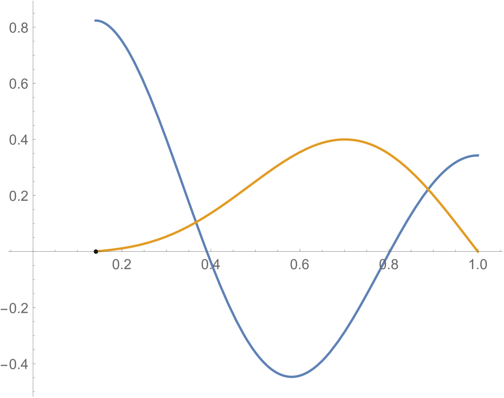
Figure 2. The plot of the eigenfunctions $\psi(r)$ and $\varphi(r)$ for $l=4$ and $a$, $\mu$, $\lambda$ as in (A.1). Here $r$ runs from the point $a$ to $1$.

Plugging (A.1) (together with $l=4$) in the expressions of $\mu_{0,2}^{\prime}(a)$ and $\lambda_{l,0}^{\prime}(a)$ we obtain:

$$\mu_{0,2}^{\prime}(a)=105.971\dots,\qquad\lambda_{4,0}^{\prime}(a)=0.12067\dots$$

The transversality condition (T) is clearly satisfied.

We now see (numerically) that in the case (A.1), indeed $\mu=\lambda$ corresponds to the eigenvalue $\mu(18)$, with $\mu(k):=\mu_{k}(\Omega_{a_{4}})$. We need to compare the value $\mu$ given in (A.1) with the other eigenvalues $\mu_{l,k}(a)$.

First, note that $\mu\equiv\mu_{0,2}>\mu_{0,i}$ for $i=0$ or $i=1$. Moreover, by Lemma 2.1, $\mu_{0,2}=\lambda_{1,1}>\mu_{1,1}$. On the other hand, with our choice of $a$, $\mu_{0,2}=\lambda_{4,0}>\mu_{i,0}$ for $i\leqslant 4$. Next, we need to compute $\mu_{l,0}(a)$ with $l\geqslant 5$, and also $\mu_{1,l}(a)$ with $l\geqslant 2$, where $a$ is given in (A.1). For that, we solve

(A.2) $$\psi^{\prime\prime}+\frac{\psi^{\prime}}{r}-l^{2}\frac{\psi}{r^{2}}+\bar{\mu}\,\psi=0\quad\text{in }(a,1)\,,\qquad\psi^{\prime}(1)=0\,,$$

where $\bar{\mu}$ is real parameter. The function $\psi$ is given by

$$\psi(r)=\frac{J_{l}(\sqrt{\bar{\mu}}r)Y_{l-1}(\sqrt{\bar{\mu}})-Y_{l}(\sqrt{\bar{\mu}}r)J_{l-1}(\sqrt{\bar{\mu}})-J_{l}(\sqrt{\bar{\mu}}r)Y_{l+1}(\sqrt{\bar{\mu}})+Y_{l}(\sqrt{\bar{\mu}}r)J_{l+1}(\sqrt{\bar{\mu}})}{Y_{l-1}(\sqrt{\bar{\mu}})-Y_{l+1}(\sqrt{\bar{\mu}})}\,.$$

The eigenvalues $\mu_{l,i}$ are obtained as the values of $\bar{\mu}$ for which $\psi^{\prime}(a)=0\,.$ The index $i$ is determined by the number of times that the corresponding eigenfunction changes sign. Using Mathematica, it is easy to find

$$\mu_{5,0}=41.1601\dots,\quad\mu_{6,0}=56.2689\dots,\quad\mu_{7,0}=73.5792\dots,\quad\mu_{1,2}=44.0466\dots,\ \ \mu_{1,3}=64.1201\dots\,.$$

Therefore, $\mu_{l,0}<\mu_{0,2}$ if and only if $l\leqslant 6$, and $\mu_{1,l}\leqslant\mu_{0,2}$ if and only if $l\leqslant 2$. As the eigenvalues $\mu_{0,0}$, $\mu_{0,1}$ have multiplicity 1 (because they correspond to radial eigenfunctions) and the rest have multiplicity 2 (since the corresponding eigenspace is spanned by the radial function multiplied by $\sin(l\theta)$ and $\cos(l\theta)$), we conclude that $\mu_{0,2}=\mu_{18}(\Omega_{a_{4}})$. Here we have used that, of course $0=\mu_{0,0}=\mu_{0}(\Omega)$. ∎

References

- [1] P. Aviles, Symmetry theorems related to Pompeiu’s problem, Amer. J. Math. 108 (5) (1986), 1023–1036.
- [2] C. Berenstein, An inverse spectral theorem and its relation to the Pompeiu problem, J. Anal. Math. 37 (1980), 128–144.
- [3] C. Berenstein and P. Yang, An inverse Neumann problem, J. Reine Angew. Math. 382 (1987), 1–21.
- [4] L. Brown, B. M. Schreiber and B. A. Taylor, Spectral synthesis and the Pompeiu problem, Ann. Inst. Fourier (Grenoble) 23 (1973), 125–154
- [5] J. Byeon, H. Huh and J. Seok, On standing waves with a vortex point of order N for the nonlinear Chern-Simons-Schrödinger equations, J. Differential Equations 261 (2016), no. 2, 1285–1316.
- [6] L. Chakalov, Sur un problème de D. Pompeiu, Annuaire Godisnik Univ. Sofia Fac.Phys.-Math., Livre 1, 40 (1944) 1–14.
- [7] S.-Y. Cheng, Eigenfunctions and nodal sets, Comm. Math. Helvetici 51 (1976), 43–55.
- [8] M. Crandall and P. Rabinowitz, Bifurcation from simple eigenvalues, J. Funct. Anal. 8 (1971), 321–340.
- [9] J. Deng, Some results on the Schiffer conjecture in , J. Differential Equations 253 no. 8 (2012), 2515–2526.
- [10] M. M. Fall, I. A. Minlend and T. Weth, The Schiffer problem on the cylinder and on the 2-sphere, arXiv:2303.17036.
- [11] N. Filonov, On an inequality between Dirichlet and Neumann eigenvalues for the Laplace operator, St. Petersburg Math. J. 16 (2005), no. 2, 413–416.
- [12] L. Friedlander, Some inequalities between Dirichlet and Neumann eigenvalues. Arch. Rat. Mech. Anal., 116 (1991), 153–160.
- [13] J. Gómez-Serrano, J. Park and J. Shi, Existence of non-trivial non-concentrated compactly supported stationary solutions of the 2D Euler equation with finite energy, Mem. Amer. Math. Soc., in press.
- [14] J. Gómez-Serrano, J. Park, J. Shi and Y. Yao, Symmetry in stationary and uniformly-rotating solutions of active scalar equations, Duke Math. J., 170 (2021), no. 13, 2957–3038.
- [15] F. Hamel, N. Nadirashvili, Circular flows for the Euler equations in two-dimensional annular domains, and related free boundary problems, J. Eur. Math. Soc., in press.
- [16] T. Kato, Perturbation theory for linear operators, Springer, Berlin, 2012.
- [17] B. Kawohl and M. Lucia, Some results related to Schiffer’s problem, J. Analyse Math. 142 (2020), 667–696.
- [18] H. Kielhöfer, Bifurcation Theory: An Introduction with Applications to PDEs, Springer, Berlin, 2004.
- [19] D. Kinderlehrer and L. Nirenberg, Regularity in free boundary problems, Ann. Sc. Norm. Sup. Pisa Cl. Sci. 4(2) (1977), 373–391.
- [20] G. Liu, Symmetry results for overdetermined boundary value problems of nonlinear elliptic equations, Nonlinear Anal. 72 (2010), 3943–3952.
- [21] M. Musso, F. Pacard, J. Wei, Finite-energy sign-changing solutions with dihedral symmetry for the stationary nonlinear Schrödinger equation, J. Eur. Math. Soc. 14 (2012) 1923–1953.
- [22] D. Pompeiu, Sur certains systèmes d’équations linéaires et sur une propriété intégrale des fonctions de plusieurs variables, Comptes Rendus de l’Académie des Sciences, Série I, 188 (1929), 1138-–1139.
- [23] W. Reichel, Radial symmetry by moving planes for semilinear elliptic BVPs on annuli and other non-convex domains, Progress in Partial Differential Equations: Elliptic and Parabolic Problems, Pitman Res. Notes 325 (1995), 164–182.
- [24] D. Ruiz, Symmetry Results for Compactly Supported Steady Solutions of the 2D Euler Equations, Arch. Ration. Mech. Anal. 247 (2023), no. 3, Paper No. 40, 25 pp.
- [25] K.T. Smith, D.C. Solmon and S.L. Wagner, Practical and mathematical aspects of the problem of reconstructing objects from radiographs, Bull. Amer. Math. Soc. 83 (1977), 1227–1270.
- [26] R. Souam, Schiffer Problem and an Isoperimetric Inequality for the First Buckling Eigenvalue of Domains on , Ann. Global Anal. and Geom. 27 (2005), 341–354.
- [27] S. A. Williams, A partial solution to the Pompeiu problem, Math. Ann. 223-2 (1976), 183–190.
- [28] N. B. Willms and G. M. L. Gladwell, Saddle points and overdetermined problems for the Helmholtz equation, Z. angew Math. Phys. 45 (1994), 1–26.
- [29] S.–T. Yau, Problem section, Seminars on Differential Geometry, Ann. of Math. Stud. 102 (1982), 669–706.
- [30] L. Zalcman, A bibliographic survey of the Pompeiu problem, Approximation by Solutions of Partial Differential equations, Kluwer, Dordrecht (1992), 185–194.