Mean-field games of speedy information access
with observation costs

Abstract

We investigate a mean-field game (MFG) in which agents can exercise control actions that affect their speed of access to information. The agents can dynamically decide to receive observations with less delay by paying higher observation costs. Agents seek to exploit their active information gathering by making further decisions to influence their state dynamics to maximize rewards. In the mean field equilibrium, each generic agent solves individually a partially observed Markov decision problem in which the way partial observations are obtained is itself also subject of dynamic control actions by the agent. Based on a finite characterization of the agents’ belief states, we show how the mean field game with controlled costly information access can be formulated as an equivalent standard mean field game on a suitably augmented but finite state space. We prove that with sufficient entropy regularisation, a fixed point iteration converges to the unique MFG equilibrium and yields an approximate $\epsilon$-Nash equilibrium for a large but finite population size. We illustrate our MFG by an example from epidemiology, where medical testing results at different speeds and costs can be chosen by the agents.

1 Introduction

In decision making, one often has the opportunity to improve the quality of one’s observations by expending extra resources. For example, medical laboratories can invest in infrastructure to reduce waiting times for testing results, to enable faster diagnosis and treatment for patients. Balancing such trade-off between information acquisition and the associated costs may be as important as selecting the course of further actions which optimise one’s rewards.

We introduce a novel mean-field game (MFG) model in discrete-time, in which agents actively control their speed of access to information. The MFG considered can be viewed as a partial observation problem, in which the information stream is not exogeneously given but rather dynamically controlled by the agents. In the game, agents can adjust their speed of information access with suitable costly efforts, and exploit their dynamic information stream to inform the choice of controls for the state dynamics so as to maximise their rewards. We utilise the information structure to construct a suitable augmentation of the state space, which includes the belief state as well as past actions taken within the dynamic delay period, that serves as the finite state space of an equivalent mean field game of standard form. Thereby, numerical schemes for discrete MFGs can be employed to compute approximate mean-field Nash equilibria (MFNE) for our MFG of speedy information access with controlled observations.

This paper covers three themes: (1) actively controlled observation delay, (2) observation costs, and (3) the analysis of an associated MFG incorporating the combination of those two features. Standard Markov decision process (MDP) frameworks assume that state observations are received instantaneously, with corresponding actions in response being also applied instantaneously. This limits the applicability of such models in many real-life situations. It is often the case that observation delay arises due to inherent features of a system, or practical limitations from data collection. For example, the times to receive medical diagnosis test results depend on the processing time required for laboratory analysis. In high-frequency trading, observation delay occurs in the form of latency, aggregated over the multiple stages of communication with the exchange [10].

There has been a large amount of literature involving the modelling of observation delays, with applications in (but not limited to) network communications [1, 2], quantitative finance [10, 8, 30] and reinforcement learning [11, 38, 28]. Most models involve an MDP framework with either a constant or random observation delay, both of which are exogenously given by the system. Both constant and random observation delay MDPs can be modelled as a partially observable MDP (POMDP) via state augmentation [5, 3, 24, 28]. It has also been shown that action delays can be considered as a form of observation delay, under a suitable transformation of the MDP problem [24]. The continuous-time counterpart with an associated HJB-type master equation has been studied in [37].

In many formulations of optimisation problems in MDPs, the information source is fixed a priori. However, it is often desirable to control the observations that one receives, in addition to the dynamics of the underlying process. This frequently occurs in resource-constrained environments where frequent measurements or sampling are either too expensive or impractical. Applications include efficient medical treatment allocation [40], environmental management [42, 43, 44, 45], communications sampling [20, 16], optimal sensing [29, 41, 39], reinforcement learning [6, 25, 7], and much more. We shall refer to these as observation cost models (OCMs). In OCM problems, the user can opt to receive an observation of the current state of the process, at the price of an observation cost which is included in the reward functional to be optimised.

The OCM can equivalently be characterised as a POMDP, by including the time elapsed, together with the last observed states and actions applied to form an augmented Markov system. In many cases, a reasonable simplification is to assume constant actions between observations [33, 23]. This leads to a finite dimensional characterisation of the augmented state, and allows efficient computation of the resulting system of quasi-variational inequalities via a penalty scheme [33]. Analysis for the more general non-constant action case has generally been restricted to the linear-quadratic Gaussian case [41, 39, 12].

In stochastic games, the computation of Nash equilibria is often intractable for large number of players. Mean-field games (MFGs), first introduced in [26] and [9], provide a way of seeking approximate Nash equilibria, by assuming symmetric interactions between agents that can be modelled by a mean-field term, in the form of a measure flow. MFGs can be treated as an asymptotic approximation of a game with large number of interacting players. Finding a mean-field Nash equilibrium (MFNE) amounts to a search for an optimal policy for a representative player, and ensuring that the state distribution of said player under such a policy is consistent with the postulated law of the other players, given by the measure flow. In discrete time, the existence of MFNE has been established in [34]. Analysis has also appeared for several model variants such as risk-sensitive criteria [36], partially observable systems [35, 36] and unknown reward/transition dynamics [18].

In general, finite MFGs suffer from non-uniqueness of MFNE and non-contractivity of the naively iterated fixed point algorithm [13]. Several algorithms have emerged to address the efficient computation of MFNEs. Entropy regularisation exploits the duality between convexity and smoothness to achieve contractivity, by either incorporating the entropy term directly into the reward functional, or imposing softmax policies during the optimisation step [14, 4, 13]. Fictitious play schemes aim to smooth the mean-field updates by averaging new iterates over the past mean-field terms, effectively damping the update to aid numerical convergence [32]. Online mirror descent further decreases computational complexity by replacing best response updates with direct $Q$-function computations [31]. In contrast, [19] reformulates the problem of searching an MFNE to an equivalent optimisation problem, allowing a possible search for multiple MFNE with standard gradient descent algorithms. We refer to the survey [27] for a comprehensive overview of the above algorithms.

Our work. We model agents’ strategic choices for speed of information access in the game, by studying a novel MFG where the speed of access is in itself also a part of the costly control. Throughout the paper, we assume that both the state and action spaces are finite. The agents participating in the game have control over two aspects: the time period of their observation delay, and their actions that influence their rewards and transition dynamics. The agent can choose over a given finite set of delay periods, with each value being associated to an observation cost. A higher observation cost corresponds to a shorter delay period, and vice versa.

Our framework here differs from existing works, in that the delay period is not exogeneously given as in the constant case[3, 5], nor is it a random variable with given dynamics as in the stochastic case [28, 10, 11]. Instead, the length of the delay is dynamically and actively decided by the agent, based on the trade-off between the extra cost versus the accuracy of more speedy observations, the latter of which can be exploited though better informed control of the dynamics and hence higher rewards. The choice of the delay period becomes an extra part of the control in the optimisation problem in tandem with the agent’s actions. When considering this as a single agent problem, which occurs during the optimisation step when the measure flow is fixed, we refer to it as a Markov Controllable Delay model (MCDM). The MCDM can be reformulated in terms of a POMDP, by augmenting the state with the most recent observation and actions taken since, to form a Markovian system. This allows the formulation of dynamic programming to obtain the Bellman equation.

When viewed as part of the overall MFG, the partial information structure of the problem implies that the measure flow should be specified on the augmented space for the fixed point characterisation of the mean field Nash equilibira (MFNE). However, the underlying transition dynamics and reward structure would depend on the distribution of the states at the present time. In the models of [35, 36], the mapping from measures on the augmented space to measures on the underlying state is given by taking the barycenter of the measure. However, our model here differs in two aspects. Firstly, although the belief state is an element of the simplex on the underlying state space, we find a finite parameter description (the state last observed and actions taken thereafter) to establish the MFG on a finitely augmented space. Secondly, due to the delayed structure, the observation kernel depends on the distribution of the states throughout each moment in time across the delay period. Thus, taking an average of a distribution over the augmented space of parameters, as a barycenter map would do, is not applicable here. Instead, we explicitly map a measure flow on the augmented space to a sequence of measures on the underlying states. Intuitively, this corresponds to an agent estimating the distribution of the current states of the population, given the observations he/she possesses (i.e., the distribution of the delay period amongst agents, and the states and actions given such a delay). We detail the construction of the MCDM in Section 2 and the corresponding MFG formulation, which we will also refer to as the MFG-MCDM, with its MFNE definition in Section 3.

The second part of this paper focuses on the computation of an MFNE for the MFG of control of information speed. We employ the popular entropy regularisation technique, which aids convergence of the classical iterative scheme: computing an optimal policy for a fixed measure flow, followed by computing the law of the player under said policy. In the standard MFG model, it is shown that the fixed point operator for the regularised problem is contractive under mild conditions [4, 13]. This forms the basis of the prior descent algorithm, which is one of the current state-of-the-art algorithms for the computation of approximate Nash equilibria for MFGs [13, 17]. We prove that for our MFG model of control of information speed, the corresponding fixed point operator also converges when it is sufficiently regularised by an entropy term. This can be summarised in the following theorem, which is a condensed version of 4.8.

Theorem 1.1.

Let $\Phi^{\mathrm{reg}}_{\eta}$ be the regularised best-response map, with regulariser parameter $\eta$, and let $\Psi^{\mathrm{aug}}$ be the measure-flow map. Then for $\eta>c_{\eta}$, there exists a unique fixed point for $\Psi^{\mathrm{aug}}\circ\Phi^{\mathrm{reg}}_{\eta}$, i.e. there exists a unique regularised MFNE for the MFG-MCDM problem. Here $c_{\eta}$ is a constant that only depends on the Lipschitz constants and bounds of the transition kernels and rewards functions.

We defer the precise definitions of the operators $\Phi^{\mathrm{reg}}_{\eta}$ and $\Psi^{\mathrm{aug}}$, as well as the constant $c_{\eta}$ to Section 4. We investigate the infinite horizon discounted cost problem with time-dependent measure flows. This extends the result in [13] for finite horizon problems, and the result in [4] for infinite horizon problems with stationary measure flows. As the MFG-MCDM is a partially observable problem, the proof also requires a crucial extra step to demonstrate that the aforementioned mapping of the measure flow on the augmented space to that on the underlying space is Lipschitz, in other to prove the required contraction.

The contributions of this paper can be summarised as follows.

1. We show dynamical programming for a Markov Controllable Delay model (MCDM), an MDP model where an individual agent can exercise dynamic control over the latency of their observations, with less information delay being more costly. The problem is cast in terms of a partially observed MDP (POMDP) with controlled but costly partial observations, for which the belief state can be described by a finite parametrization. Solving this POMDP is shown to be equivalent to solving a finite MDP on an augmented finite state space, whose extension also involves past actions taken during the (non-constant but dynamically controlled) delay period.

2. We introduce a corresponding Mean Field Game (MFG) where speedy information access is subject to the agents’ strategic control decisions. For a fixed measure flow, which describes the statistical population evolution, the ensuing single agent control problem becomes an MCDM. Although a mean-field Nash equilibrium (MFNE) is defined in terms of the augmented space, the underlying dynamics and rewards still depend on the underlying state distribution. We show how a measure flow on the underlying space is determined and computed from that of the augmented space. This construction exploits the finite parameterization of the belief state; whereas the barycenter approach for belief state which are measure-valued as in [35] does not apply here.

3. By using a sufficiently strong entropy regularisation in the reward functional, we prove that the regularised MFG-MCDM has a unique MFNE which is described by a fixed point, and can serve as an approximate Nash equilibrium for a large but finite population size. The characterisation of the MCDM as a finite MDP enables to compute the Nash equilibrium of the corresponding MFG, by using methods from [4, 13]. The results also extend to a MFG formulated on infinite horizon with time-dependent measure flows.

4. We demonstrate our model by an epidemiology example, in which we compute both qualitative effects of information delay and cost to the equilibrium, and also the quantitative properties of convergence relating to the entropy regularisation. For computation, we employ the Prior Descent algorithm [13], applying the new mfglib Python package [17] to our partially observable model.

The remainder of the paper is organized as follows. Section 2 develops the formulation of the MCDM as a POMDP and establishes dynamic programming on the augmented space. Section 3 explains the corresponding MFG setup, the fixed point characterisation of the equilibrium, and shows some basic properties. Section 4 establishes the contraction property of the fixed point iteration map for the regularised mean field game and its ability to yield an approximate equilibrium for the finite player game. Finally, Section 5 demonstrates a numerical example from epidemiology for illustrtration.

1.1 Notation and preliminaries

For any finite set $E$, we identify the space of probability measures on $E$ with the simplex $\Delta_{E}$. We equip $\Delta_{E}$ with the metric $\delta_{TV}$ induced by the total variation norm on the space of signed measures. That is,

$$\delta_{TV}(p,\hat{p})=\lVert p-\hat{p}\rVert_{TV}=\frac{1}{2}\sum_{e\in E}\lvert p(e)-\hat{p}(e)\rvert,\qquad p,\hat{p}\in\Delta_{E}.$$

We will generally be considering Markovian policies in this paper. A Markovian policy $\pi=(\pi_{t})_{t}$ is then a sequence of maps $\pi_{t}:E\to\Delta_{{E}^{\prime}}$, mapping a finite set $E$ to the simplex on another finite set ${E}^{\prime}$. Since a policy is bounded, we equip it with the sup norm

$$\delta_{\Pi}(\pi,\hat{\pi})=\sup_{t\geq 0}\max_{e\in E}\delta_{TV}(\pi_{t}(\cdot\mid e),\hat{\pi}_{t}(\cdot\mid e)).$$

Let $\Delta_{E}^{T}$ denote the space of measure flows on $E$, with $T\in\mathbb{N}\cup\{\infty\}$. If $T$ is finite, we equip $\Delta_{E}^{T}$ with the sup metric

$$\delta_{\mathrm{max}}(\bm{\mu},\bm{\hat{\mu}})=\max_{0\leq t\leq T}\delta_{TV}(\mu_{t},\hat{\mu}_{t}),\quad\bm{\mu},\bm{\hat{\mu}}\in\Delta^{T}_{E}.$$

If $T=\infty$, we instead use the metric

$$\delta_{\infty}(\bm{\mu},\bm{\hat{\mu}})=\sum^{\infty}_{t=1}\zeta^{-t}\delta_{TV}(\mu_{t},\hat{\mu}_{t}),\quad\bm{\mu},\bm{\hat{\mu}}\in\Delta^{\infty}_{E},$$ (1.1)

where $\zeta>1$. Note that the choice of $\zeta$ is not canonical, and as long as $\zeta>1$, $\delta_{\infty}$ induces the product topology on $\Delta_{E}^{\infty}$, which is compact by Tychonoff’s theorem, since each individual simplex $\Delta_{E}$ is also compact. Hence $(\Delta_{E}^{\infty},\delta_{\infty})$ is a complete metric space. This allows us to appeal to Banach’s fixed point theorem when considering the contraction mapping arguments later.

We will often consider a sequence of actions taken, e.g. $a_{1},\ldots,a_{n}\in A$. In these cases we will use the shorthand notation $(a)^{n}_{1}=(a_{1},\ldots,a_{n})$. We will use both notations interchangebly throughout the rest of this paper.

We will frequently make use of the following proposition in our analysis.

Proposition 1.2 ([15, p.141]).

For any real valued function $F$ on a finite set $E$, given $\nu,\nu^{\prime}\in\Delta_{E}$ we have the inequality (see also proof of [4, Proposition 1])

$$\left\lvert\sum_{e\in E}F(e)\nu(e)-\sum_{e\in E}F(e)\nu^{\prime}(e)\right\rvert\leq\lambda(F)\ \delta_{TV}(\nu,\nu^{\prime}),$$

where $\lambda(F)\coloneqq\max_{e\in E}F(e)-\min_{e\in E}F(e)$.

2 MDPs with controllable information delay

We first state the definition of a Markov controllable delay model (MCDM) below, which characterises the scenarios where agents can control their information delay.

Definition 2.1.

A Markov controllable delay model (MCDM) is a tuple $\langle\mathcal{X},A,\mathcal{D},\mathcal{C},p,r\rangle$, where

• $\mathcal{X}$ is the finite state space;

• $A$ is the finite action space;

• $\mathcal{D}=\{d_{0},\ldots,d_{K}\}$, with $0\leq d_{K}<\ldots<d_{0}$, is the set of delay values;

• $\mathcal{C}=\{c_{0},c_{1},\ldots,c_{K}\}$, with $0=c_{0}<c_{1}\ldots<c_{K}$, is the set of cost values;

• $p:\mathcal{X}\times A\to\Delta_{\mathcal{X}}$ is the transition kernel;

• $r:\mathcal{X}\times A\to[0,\infty)$ is the one-step reward function.

Let us also denote the $n$-step transition probabilities by $p^{(n)}(\ \cdot\mid x,(a)^{n}_{1})$, where we use the notation $(a)^{n}_{1}\coloneqq(a_{1},\ldots,a_{n})\subset A$. For a given set of delay values $\mathcal{D}$, define also

• $\overline{\mathcal{D}}\coloneqq[d_{K},d_{0}]=\{d_{K},d_{K}+1,\ldots,d_{0}\}$.

• The intervention variables $(i_{t})_{t}$, taking values in the intervention set $\mathcal{I}\coloneqq\{0,1,\ldots,K\}$.

$\mathcal{D}$ represents the delay values that an agent can choose from, with $(i_{t})_{t}$ representing the decision on the choice of delay, and $\overline{\mathcal{D}}$ represents the range of delay values of the system at any given point in time. A value of $i_{n}=k$ indicates that at time $n$ the agent wishes to pay a cost of $c_{k}$ to change their delay to $d_{k}$ units. To ensure that the setup is well-defined, if $i_{n}=k$ and the current delay $d$ is shorter than $d_{k}$, then the delay at time $n+1$ will simply be extended to $d+1$ units (in reality, paying a higher cost for a longer delay is clearly sub-optimal, so such a choice of $i_{n}$ would not practically occur).

Formally, the MCDM evolves sequentially as follows. Suppose at time $t$, the controller observes the underlying state $x_{t-d_{0}}\in\mathcal{X}$, with knowledge of their actions $a_{t-d_{0}},\ldots,a_{t-1}\in A$ applied since. Based on this information, the controller applies an action $a_{t}$ and receives a reward $r(x_{t},a_{t})$ (which we assume not to be observable until $x_{t}$ becomes observable). The controller then decides on the choice of cost $c_{i}$, which determines their next delay period of $d_{i}$ units, i.e. observing $x_{t+1-d_{i}}$ at time $t+1$. This process then repeats at the next time. If no cost is paid, then no new observations occur, until the delay reaches $d_{0}$ units again. Figure 2.1 depicts a typical evolution of an MCDM.

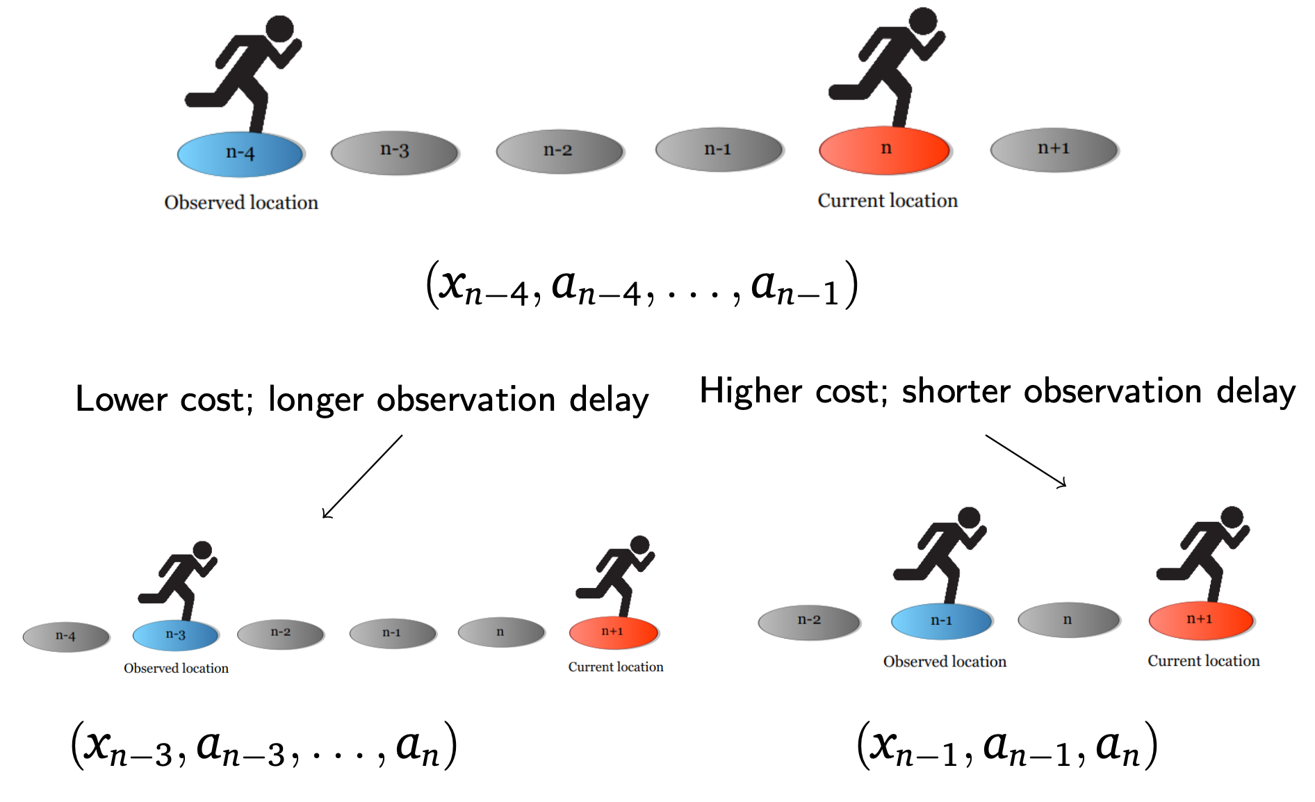
Figure 2.1: Control of information speed

The precise construction can be set up as follows. We assume that the problem initiates at time $t=0$, and denote prior observations with negative indices.

Definition 2.2.

Define the history sets $\{H_{t}\}_{t\geq 0}$ as follows: let $H_{0}\coloneqq\overline{\mathcal{D}}\times(\mathcal{X}\times A)^{d_{0}}\times\mathcal{X}$, denoting its elements in the form of $h_{0}=(d,x_{-d_{0}},a_{-d_{0}},\ldots,x_{-1},a_{-1},x_{0})$. Then, define recursively

$$H_{t}\coloneqq H_{t-1}\times A\times\mathcal{I}\times\mathcal{X},\quad t\geq 1.$$

The canonical sample space is

$$\Omega\coloneqq H_{\infty}\coloneqq H_{0}\times(A\times\mathcal{I}\times\mathcal{X})^{\infty}.$$

A policy $\pi=(\pi_{t})_{t\geq 0}$ is a sequence of kernels $\pi_{t}:H_{t}\to\Delta_{A\times\mathcal{I}}$. Then, given an initial distribution $q_{0}\in\Delta_{H_{0}}$ and a policy $\pi$, the Ionescu-Tulcea theorem [21, Appendix C] gives a unique probability measure $\mathbb{P}^{\pi}_{q_{0}}$ such that for $\omega=(d,x_{-d_{0}},a_{-d_{0}},\ldots,x_{0},a_{0},i_{0},x_{1},a_{1},i_{1},\ldots)$,

$$\mathbb{P}^{\pi}_{q_{0}}(\omega) =q_{0}(h_{0})\ p(x_{-d_{0}+1}\mid x_{-d_{0}},a_{-d_{0}})\ldots p(x_{0}\mid x_{-1},a_{-1})$$

$$\qquad\pi_{0}(a_{0},i_{0}\mid d,x_{-d_{0}},a_{-d_{0}},\ldots,x_{0})\ p(x_{1}\mid x_{0},a_{0})\ldots$$

The value $d$ appearing in $H_{0}$ represents the initial delay period. Given a history sequence $h_{t}\in H_{t}$, subsequent delay periods at time $t>0$ can be deduced from the values of $d$ and $(i_{n})^{t-1}_{n=0}$. Denote this value by $d(t)\in\overline{\mathcal{D}}$. This leads to the following definition for the set of admissible policies.

Definition 2.3.

A policy $\pi$ is admissible for an MCDM if at each time $t$, there exists a sequence of kernels $\phi^{d}_{t}:\mathcal{X}\times A^{d}\to\Delta_{A\times\mathcal{I}}$, $d\in\overline{\mathcal{D}}$, such that for each $h_{t}\in H_{t}$,

$$\pi_{t}(\cdot\mid h_{t})=\phi^{d(t)}_{t}(\cdot\mid x_{-d_{0}},\ldots,x_{t-d_{h_{t}}},a_{-d_{0}},\ldots,a_{t-1}),$$

where $d(t)\in\overline{\mathcal{D}}$ is the delay period at time $t$ for a corresponding history sequence $h_{t}\in H_{t}$. The set of admissible policies for the MCDM is denoted by $\Pi_{DM}$.

Given the MCDM $\langle\mathcal{X},A,\mathcal{D},\mathcal{C},p,r\rangle$ and an admissible policy $\pi\in\Pi_{DM}$, the objective function for the infinite horizon problem with discounted cost is

$$J(\pi)\coloneqq\mathbb{E}^{\pi}_{q_{0}}\left[\sum^{\infty}_{n=0}\gamma^{n}\left(r(x_{n},a_{n})-\sum^{K}_{k=1}c_{k}\mathbbm{1}_{\{i_{n}=k\}}\right)\right],$$

where $\mathbb{E}^{\pi}_{q_{0}}$ is the expectation over the measure $\mathbb{P}^{\pi}_{q_{0}}$, and $\gamma\in(0,1)$ is the discount factor.

The search for an optimal $\pi\in\Pi_{DM}$ can be solved by considering an equivalent MDP on an augmented state, which contains all the information that occurred between the current time and the delayed time. As noted in [3] for the constant delay case, the lifting is akin to the classical POMDP approach on constructing an equivalent MDP on the belief state, but in this case the ‘observations’ do not come from an exogenous information stream, but from a past occurred state instead.

For a full Markovian system, the augmented variable will include the delay of the system at the current time, the underlying state that is observed with that delay, and the actions applied from that moment until the present. This will be presented as the following.

Definition 2.4.

Given the delay values $\mathcal{D}=\{d_{0},\ldots,d_{K}\}$, define the augmented space $\mathcal{Y}$ by

$$\mathcal{Y}\coloneqq\bigcup_{d=d_{K}}^{d_{0}}\{d\}\times\mathcal{X}\times A^{d},$$

where $\overline{\mathcal{D}}=[d_{K},d_{0}]$. Then an element $y\in\mathcal{Y}$ can be written in the form

$$(d,x,a_{-d},\ldots,a_{-1}),\ \mbox{or }(d,x,(a)^{-1}_{-d}),$$

where negative indices are used to indicate that the actions had occurred in the past. If specific indices are not required, we will also use the notation $y=(d,x,\bm{a})$.

Although the length of the delay is implicit from the number of elements in $\bm{a}$, we explicitly include $d$ in $\mathcal{Y}$ for simpler comprehension.

Remark 2.5.

As the length of the delay is variable and dependent on the control, the dimension of the augmented state is also variable. In practice, during computation, we can keep the dimensions consistent by introducing dummy variables $\varnothing$. This follows the treatment of stochastic delays in [28]. Specifically. for any set $E$ we write $E_{\varnothing}=E\cup\{\varnothing\}$. Then an element $y\in\mathcal{Y}$ can be embedded into the space $\mathcal{X}\times A^{d_{0}}_{\varnothing}$ via the mapping

$$(d,x,(a)^{-1}_{-d})\mapsto(x,(a)^{-1}_{-d},\underbrace{\varnothing,\ldots,\varnothing}_{\text{$d_{0}-d$ units}}).$$

We can now construct the MDP on the augmented space. For $y=(d,x,\bm{a}),\hat{y}=(\hat{d},\hat{x},\hat{\bm{a}})\in\mathcal{Y}$, $a^{\prime}\in A$, and $i\in\mathcal{I}$, let $p_{y}:\mathcal{Y}\times(A\times\mathcal{I})\to\Delta_{\mathcal{Y}}$ be the augmented kernel, where

$$p_{y}(\hat{y}\mid y,a^{\prime},i) =\begin{cases}p^{(d-d_{i}+1)}\big{(}\hat{x}\mid x,(a)_{-d}^{-d_{i}}\big{)}\ \mathbbm{1}_{\left\{\hat{d}=d_{i},\ \hat{\bm{a}}=\left((a)_{-d_{i}+1}^{-1},a^{\prime}\right)\right\}}\ ,&\ d_{i}\leq d\leq d_{0};\\ \mathbbm{1}_{\left\{\hat{x}=x,\ \hat{d}=d+1,\ \hat{\bm{a}}=\big{(}(a)^{-1}_{-d},a^{\prime}\big{)}\right\}}\ ,&\ d_{K}\leq d<d_{i}.\end{cases}$$ (2.1)

Let ${\Pi}^{\prime}$ denote the set of policies for this augmented MDP. That is, ${\pi}^{\prime}=({\pi}^{\prime}_{t})\in{\Pi}^{\prime}$ is such that ${\pi}^{\prime}_{t}:{H}^{\prime}_{t}\to\Delta_{A\times\mathcal{I}}$, where ${H}^{\prime}_{0}\coloneqq\mathcal{Y}$ and ${H}^{\prime}_{t}\coloneqq{H}^{\prime}_{t-1}\times A\times\mathcal{I}\times\mathcal{Y}$ for $t\geq 1$. By the Ionescu-Tulcea theorem again, for an initial distribution $q_{y_{0}}\in\Delta_{\mathcal{Y}}$ and a policy ${\pi}^{\prime}\in{\Pi}^{\prime}$, there exists a unique probability measure $\mathbb{P}^{{\pi}^{\prime}}_{q_{y_{0}}}$ such that

$$\mathbb{P}^{{\pi}^{\prime}}_{q_{y_{0}}}(y_{0},a_{0},i_{0},y_{1},\ldots)=q_{y_{0}}(y_{0})\ {\pi}^{\prime}_{0}(a_{0},i_{0}\mid y_{0})\ p_{y}(y_{1}\mid y_{0},a_{0},i_{0})\ldots$$ (2.2)

It is then straightforward to see that there is a one-to-one correspondence between policies in the original MCDM and policies in the augmented MDP. This follows analogously from the case of a fixed information delay [3], and we summarise the argument here: each $h_{t}\in H_{t}$ can be mapped to a corresponding ${h}^{\prime}_{t}\in{H}^{\prime}_{t}$ via

$$(d,x_{-d_{0}},a_{-d_{0}},\ldots,x_{0},a_{0},i_{0},\ldots,x_{t-1},a_{t-1},i_{t-1},x_{t})\mapsto(y_{0},a_{0},i_{0},\ldots,y_{t-1},a_{t-1},i_{t-1},y_{t})$$

where $y_{t}=\Big{(}d(t),x_{t-d(t)},(a)_{t-d(t)}^{t-1}\Big{)}$ for $t\geq 0$. Then, given a policy $\pi\in\Pi_{DM}$, one can define a policy ${\pi}^{\prime}\in{\Pi}^{\prime}$ via

$${\pi}^{\prime}_{t}(\cdot\mid{h}^{\prime}_{t})=\pi_{t}(\cdot\mid h_{t}),\quad t\geq 0.$$

Moreover, the policies $\pi$ and ${\pi}^{\prime}$ assign the same joint law to $(y_{t},a_{t},i_{t})_{t\geq 0}$ (when viewed as the canonical coordinate projection). One can then consider the objective function in the augmented space $\mathcal{Y}$, which is now a fully observable problem:

$${J}^{\prime}({\pi}^{\prime})\coloneqq\mathbb{E}^{{\pi}^{\prime}}_{q_{y_{0}}}\left[\sum^{\infty}_{n=0}\gamma^{n}r_{y}(y_{n},a_{n},i_{n})\right],\quad{\pi}^{\prime}\in{\Pi}^{\prime},$$

where $r_{y}:\mathcal{Y}\times(A\times\mathcal{I})\to[0,\infty)$ and

$$r_{y}(y,{a}^{\prime},i)=\sum_{{x}^{\prime}\in\mathcal{X}}r({x}^{\prime},{a}^{\prime})p^{(d)}({x}^{\prime}\mid x,\bm{a})-\sum^{K}_{k=1}c_{k}\mathbbm{1}_{\{i=k\}},\quad y=(x,d,\bm{a}).$$ (2.3)

The two problems are equivalent in that $\pi_{*}\in\Pi_{DM}$ is optimal for $J$ if and only if $\pi^{\prime}_{*}\in{\Pi}^{\prime}$ is optimal for ${J}^{\prime}$, and it holds that

$$\sup_{\pi\in\Pi_{DM}}J(\pi)=J(\pi_{*})={J}^{\prime}(\pi^{\prime}_{*})=\sup_{{\pi}^{\prime}\in{\Pi}^{\prime}}{J}^{\prime}({\pi}^{\prime})$$

Given the equivalence, we shall use $\Pi_{DM}$ to represent the set of admissible policies without loss of generality. This allows us to establish dynamic programming for the MCDM as follows.

Proposition 2.6.

Let $v:\mathcal{Y}\to\mathbb{R}$ be the value function

$$v(y)=\sup_{\pi\in\Pi_{DM}}\mathbb{E}^{\pi}\left[\sum^{\infty}_{n=0}\gamma^{n}r_{y}(y_{n},a_{n},i_{n})\middle|y_{0}=y\right],$$

Then $v$ satisfies the dynamic programming equation

$$v(y)=\max_{({a}^{\prime},i)\in A\times\mathcal{I}}\left\{\sum_{{x}^{\prime}\in\mathcal{X}}r({x}^{\prime},{a}^{\prime})p^{(d)}({x}^{\prime}\mid x,\bm{a})-\sum^{K}_{k=1}c_{k}\mathbbm{1}_{\{i=k\}}+\gamma\sum_{y^{\prime}\in\mathcal{Y}}p_{y}({y}^{\prime}\mid y,{a}^{\prime},i)v({y}^{\prime})\right\},$$

where $p_{y}$ is the augmented kernel as in (2.1). Moreover, the optimal policy is given in feedback form, so that $\pi_{*,n}=\phi_{n}(y_{n})$ for some feedback function $\phi_{n}$.

Proof.

This is a standard application of dynamic programming for a fully observable MDP, see e.g. [22, Theorem 4.2.3]. ∎

Remark 2.7.

When considering the MFG in the next section, a deterministic measure flow representing the population distribution introduces an implicit time dependence within the transition kernel and reward. The generic single agent problem in the definition of the MFNE then becomes time-inhomogeneous. The time-homogeneous setup in this section readily generalises directly to a setup with time-inhomogeneous transition kernels, rewards and dynamic programming equations. However, for ease of exposition we choose to present the MCDM under the time-homogeneous setting here.

3 MFG formulation with control of information speed

To ease notation, in the remainder of the paper we write $U\coloneqq A\times\mathcal{I}$ and $u=(a,i)\in U$.

3.1 Finite agent game with observation delay

Consider an $N$-player game with mean-field interaction, where each agent can control their observation delay. We shall start with incorporating the measure dependence into the MCDM in 2.1.

Definition 3.1.

An MCDM with measure dependence is a tuple $\langle\mathcal{X},A,\mathcal{D},\mathcal{C},p,r\rangle$, where

• $\mathcal{X}$ is the finite state space;

• $A$ is the finite action space;

• $\mathcal{D}=\{d_{0},\ldots,d_{K}\}$, with $0\leq d_{K}<\ldots<d_{0}$, is the set of delay values;

• $\mathcal{C}=\{c_{1},\ldots,c_{K}\}$, with $0=c_{0}<c_{1}<\ldots<c_{K}$, is the set of cost values;

• $p:\mathcal{X}\times A\times\Delta_{\mathcal{X}}\to\Delta_{\mathcal{X}}$ is the transition kernel;

• $r:\mathcal{X}\times A\times\Delta_{\mathcal{X}}\to[0,\infty)$ is the one-step reward function.

Denote by $x^{j}_{t}\in\mathcal{X}$ the state of the $j$-th player at time $t$, and $a^{j}_{t}\in A$ the corresponding action. Assume that the mean-field interaction occurs in the reward and the transition probabilities of the players, and is identically distributed for each player. The transition kernel is given by $p:\mathcal{X}\times A\times\Delta_{\mathcal{X}}\to\Delta_{\mathcal{X}}$ so that the $j$-th player moves from state $x^{j}_{t}$ to $x^{j}_{t+1}$ with probability

$$p(x^{j}_{t+1}\mid x^{j}_{t},a^{j}_{t},e^{N}_{t}),\quad e^{N}_{t}(\cdot)=\frac{1}{N}\sum^{N}_{k=1}\delta_{x^{k}_{t}}(\cdot).$$

Here $e^{N}_{t}$ is the empirical distribution of the states of the agents. Similarly, the one-step reward function is given by $r:\mathcal{X}\times A\times\Delta_{\mathcal{X}}\to[0,\infty)$ so that player $j$ receives a reward of $r(x^{j}_{t},a^{j}_{t},e^{N}_{t})$ at time $t$.

Recall that for a fully Markovian system, we consider the lifted problem in the augmented space

$$\mathcal{Y}\coloneqq\bigcup_{d=d_{K}}^{d_{0}}\{d\}\times\mathcal{X}\times A^{d}.$$

For the $N$-player model, consider the history sets $H_{0}\coloneqq\mathcal{Y}\times\Delta_{\mathcal{Y}}$ and $H_{t}\coloneqq H_{t-1}\times U\times\mathcal{Y}\times\Delta_{\mathcal{Y}}$ for $t\geq 1$. A policy $\pi=(\pi_{t})_{t\geq 0}$ is a sequence of maps $\pi_{t}:H_{t}\to\Delta_{U}$.

Definition 3.2.

A policy $\pi$ is admissible for the $N$-player MCDM if at each time $t$, there exists a sequence of kernels $\phi^{d}_{t}:\mathcal{X}\times A^{d}\times\Delta^{t}_{\mathcal{Y}}\to\Delta_{A\times\mathcal{I}}$, $d\in\overline{\mathcal{D}}$, such that for each $h_{t}\in H_{t}$,

$$\pi_{t}(\cdot\mid h_{t})=\phi^{d(t)}_{t}(\cdot\mid x_{-d_{0}},\ldots,x_{t-d_{h_{t}}},a_{-d_{0}},\ldots,a_{t-1},\tilde{e}^{N}_{0},\ldots,\tilde{e}^{N}_{t}),$$

where $d(t)\in\overline{\mathcal{D}}$ is the delay period at time $t$ for a corresponding history sequence $h_{t}\in H_{t}$, and $\tilde{e}^{N}_{t}$ is the empirical distribution of augmented state, i.e.

$$\tilde{e}^{N}_{t}=\frac{1}{N}\sum^{N}_{k=1}\delta_{y^{k}_{t}}(\cdot),\quad y^{k}_{t}=(d^{k}(t),x_{t-d^{k}(t)},a_{t-d^{k}(t)},\ldots,a_{t-1}).$$

The set of admissible policies for player $j$ is denoted by $\Pi^{j}$.

Let $\Pi=\prod^{N}_{j=1}\Pi^{j}$. Player $j$’s objective function is given by

$$J^{N}_{j}(\pi^{(N)})=\mathbb{E}^{\pi^{(N)}}\left[\sum^{\infty}_{n=0}\gamma^{n}r(x^{j}_{n},a^{j}_{n},e^{N}_{n})\right]$$

where $\pi^{(N)}=(\pi^{1},\ldots,\pi^{N})\in\Pi$. The notion of optimality in the $N$-player game can be captured by the Nash equilibrium, which intuitively says at equilibrium, no player can make gains by deviating from their current strategy, provided that all other players remain at their strategy.

Definition 3.3 (Nash equilibrium).

$\pi^{(N)}_{*}\in\Pi$ is a Nash equilibrium for the $N$-player MCDM if for each $j\in\{1,\ldots,N\}$,

$$J^{N}_{j}(\pi^{(N)}_{*})=\sup_{\pi\in\Pi^{j}}J^{N}_{j}(\pi,\pi_{*}^{-j}),$$

where $\pi^{-j}_{*}=(\pi^{1}_{*},\ldots,\pi^{j-1}_{*},\pi^{j+1}_{*},\ldots,\pi^{N}_{*})$.

Definition 3.4 ($\varepsilon$-Nash equilibrium).

For $\varepsilon>0$, a policy $\pi^{(N)}\in\Pi$ is an $\varepsilon$-Nash equilibrium for the MCDM if for each $j\in\{1,\ldots,N\}$,

$$J^{N}_{j}(\pi)\geq\sup_{\pi\in\Pi^{j}}J^{N}_{j}(\pi,\pi^{-j})-\varepsilon.$$

In general, the Nash equilibrium is hard to characterise and computationally intractable. It is also impractical to search over policies that depend on the distribution of all players. Therefore it is more useful to consider a search over Markovian policies for each player, and formulate the equilibrium condition with respect to such policies. Indeed the common approach for modelling partially observable games is to consider Markovian policies as above [35]. This is a reasonable assumption as in practice it will be hard for each agent to keep track of the movement of all other players, when the number of players grow increasingly large.

A policy is Markovian if $\pi=(\pi_{t})_{t\geq 0}$ is such that $\pi_{t}:\mathcal{Y}\to\Delta_{U}$. Let $\Pi_{\mathrm{mrkv}}^{j}$ denote the set of Markov policies for the player $j$, with $\Pi_{\mathrm{mrkv}}=\prod^{N}_{j=1}\Pi_{\mathrm{mrkv}}^{j}$.

Definition 3.5 (Markov–Nash equilibrium).

$\pi^{(N)}_{*}\in\Pi_{\mathrm{mrkv}}$ is a Markov–Nash equilibrium for the $N$-player MCDM if for each $j\in\{1,\ldots,N\}$,

$$J^{N}_{j}(\pi^{(N)}_{*})=\sup_{\pi\in\Pi_{\mathrm{mrkv}}^{j}}J^{N}_{j}(\pi,\pi_{*}^{-j}),$$

where $\pi^{-j}_{*}=(\pi^{1}_{*},\ldots,\pi^{j-1}_{*},\pi^{j+1}_{*},\ldots,\pi^{N}_{*})$.

Definition 3.6 ($\varepsilon$-Markov–Nash equilibrium).

For $\varepsilon>0$, a policy $\pi^{(N)}\in\Pi_{\mathrm{mrkv}}$ is an $\varepsilon$-Nash equilibrium for the MCDM if for each $j\in\{1,\ldots,N\}$,

$$J^{N}_{j}(\pi)\geq\sup_{\pi\in\Pi_{\mathrm{mrkv}}^{j}}J^{N}_{j}(\pi,\pi^{-j})-\varepsilon.$$

3.2 MFNE for the MFG-MCDM

The computation and characterisation of Nash equilibria is typically intractable due to the curse of dimensionality and the coupled dynamics across the different agents. Therefore, as an approximation, we consider the infinite population limit by sending the number of players ${N\to\infty}$, and replacing the empirical distribution of the agents by a measure flow ${\bm{\mu}=(\mu_{n})_{n}\in\Delta^{\infty}_{\mathcal{X}}}$. In the mean-field setting, we consider the viewpoint of one representative agent, and assume that its interactions with members of the population, modelled by the measure flow $\bm{\mu}$, are symmetric. As in the $N$-player game, we consider a tuple $\langle\mathcal{X},A,\mathcal{D},\mathcal{C},p,r\rangle$ (see 3.1). For a given measure flow $\bm{\mu}\in\Delta^{\infty}_{\mathcal{X}}$, at time $n$, a representative agent transitions from the state $x_{n}$ to a new state $x_{n+1}$ with probability

$$p(x_{n+1}\mid x_{n},a_{n},\mu_{n}),$$

and collects a reward of $r(x_{n},a_{n},\mu_{n})$. As each transition of the underlying state now depends on the given measure, the $d$-step transition kernel ${p^{(d)}:\mathcal{X}\times A^{d}\times\Delta^{d}_{\mathcal{X}}\to\Delta_{\mathcal{X}}}$ now depends on the measure flow across the $d$ time steps, so that we have

$$x_{n+d} \sim p^{(d)}(\cdot\mid x_{n},(a)_{n}^{n+d-1};(\mu)_{n}^{n+d-1}).$$ (3.1)

We impose the follow Lipschitz assumptions on the transition kernels and reward function.

Assumption 3.7.

• The one-step reward function $r$ satisfies a Lipschitz bound: there exists a constant $L_{r}$ such that for all $x,\hat{x}\in\mathcal{X}$, $a,\hat{a}\in A$, ${\mu,\hat{\mu}\in\Delta_{\mathcal{X}}}$,

  $$\lvert r(x,a,\mu)-r(\hat{x},\hat{a},\hat{\mu})\rvert\leq L_{r}\left(\mathbbm{1}_{\{x\neq\hat{x}\}}+\mathbbm{1}_{\{a\neq\hat{a}\}}+\delta_{TV}(\mu,\hat{\mu})\right).$$

• For $1\leq n\leq d_{0}$, the $n$-step transition kernels satisfy a uniform Lipschitz bound: there exists a constant $L_{p}$ such that for all $x,\hat{x}\in\mathcal{X}$, $\bm{a},\hat{\bm{a}}\in A^{n}$, ${\bm{\mu},\hat{\bm{\mu}}\in\Delta^{n}_{\mathcal{X}}}$,

  $$\delta_{TV}\left(p^{(n)}(\cdot\mid x,\bm{a},\bm{\mu}),\ p^{(n)}(\cdot\mid\hat{x},\hat{\bm{a}},\hat{\bm{\mu}})\right)\leq L_{p}\left(\mathbbm{1}_{\{x\neq\hat{x}\}}+\mathbbm{1}_{\{\bm{a}\neq\hat{\bm{a}}\}}+\delta_{\mathrm{max}}(\bm{\mu},\hat{\bm{\mu}})\right).$$

In particular, as both $\mathcal{X}$ and $A$ are assumed to be finite, and the simplex $\Delta_{\mathcal{X}}$ is compact, both the reward function $r$ and transition kernel $p$ are bounded by some constants $M_{r}$ and $M_{p}$ respectively.

Once again, we shall consider the lifted problem on the augmented space

$$\mathcal{Y}\coloneqq\bigcup_{d=d_{K}}^{d_{0}}\{d\}\times\mathcal{X}\times A^{d}.$$

Under this augmented space $\mathcal{Y}$, now with the inclusion of the measure dependence, the counterparts to $p_{y}$ and $r_{y}$ in (2.1) and (2.3) are given as follows. Let $y=\left(d,x,(a)^{n-1}_{n-d}\right)$, $\hat{y}=(\hat{d},\hat{x},\hat{\bm{a}})$, $u=(a_{n},i)$, and ${\bm{\mu}=(\mu)^{n-d_{K}}_{n-d_{0}}}$,

• ${p_{y}:\mathcal{Y}\times U\times\Delta^{d_{0}-d_{K}+1}_{\mathcal{X}}\to\Delta_{\mathcal{Y}}}$ is given by

  $$p_{y}(\hat{y}\mid y,u,\bm{\mu})$$

  $$= \begin{cases}p^{(d-d_{i}+1)}\big{(}\hat{x}\mid x,(a)_{n-d}^{n-d_{i}},(\mu)^{n-d_{i}}_{n-d}\big{)}\ \mathbbm{1}_{\left\{\hat{d}=d_{i},\ \hat{\bm{a}}=(a)_{n-d_{i}+1}^{n}\right\}}\ ,&\ d_{i}\leq d\leq d_{0};\\ \mathbbm{1}_{\left\{\hat{x}=x,\ \hat{d}=d+1,\ \hat{\bm{a}}=(a)^{n}_{n-d}\right\}}\ ,&\ d_{K}\leq d<d_{i}.\end{cases}$$ (3.2)

• The reward function $r_{y}:\mathcal{Y}\times U\times\Delta^{d_{0}+1}_{\mathcal{X}}\to[0,\infty)$ is

  $$r_{y}(y,u,\bm{\mu})=\sum_{{x}^{\prime}\in\mathcal{X}}r({x}^{\prime},a_{n},\mu_{n})p^{(d)}({x}^{\prime}\mid x,\bm{a},(\mu)^{n-1}_{n-d})-\sum^{K}_{k=1}c_{k}\mathbbm{1}_{\{i=k\}},.$$

Given Assumption 3.7, we have the following bounds in $p_{y}$ and $r_{y}$.

Proposition 3.8.

Under Assumption 3.7:

• For all $y,\hat{y}\in\mathcal{Y}$, $u,\hat{u}\in U$, $\bm{\mu},\hat{\bm{\mu}}\in\Delta^{d_{0}-d_{K}+1}_{\mathcal{X}}$, the augmented kernel $p_{y}$ satisfies the Lipschitz bound

  $$\delta_{TV}\left(p_{y}(\cdot\mid y,u,\bm{\mu}),\ p_{y}(\cdot\mid\hat{y},\hat{u},\hat{\bm{\mu}})\right)\leq L_{P}\left(\mathbbm{1}_{\{y\neq\hat{y}\}}+\mathbbm{1}_{\{u\neq\hat{u}\}}+\delta_{\mathrm{max}}(\bm{\mu},\hat{\bm{\mu}})\right).$$

  where $L_{P}=\max\{2M_{p},L_{p}\}$.

• For all $y,\hat{y}\in\mathcal{Y}$, $u\in U$, $\bm{\mu},\hat{\bm{\mu}}\in\Delta^{d_{0}+1}_{\mathcal{X}}$, the augmented reward function $r_{y}$ is in $\bm{\mu}$ and satisfies the bound:

  $$\lvert r_{y}(y,u,\bm{\mu})-r_{y}(\hat{y},u,\hat{\bm{\mu}})\rvert\leq 2L_{r}M_{p}\mathbbm{1}_{\{y\neq\hat{y}\}}+(L_{r}+c_{K}-c_{0})\mathbbm{1}_{\{u\neq\hat{u}\}}+L_{R}\ \delta_{\mathrm{max}}(\bm{\mu},\hat{\bm{\mu}}),$$

  where $L_{R}=L_{r}+L_{r}L_{p}$. Also $r_{y}$ is bounded by $M_{r}+c_{K}\eqqcolon M_{R}$.

Proof.

• We have from the triangle inequality

  $$\delta_{TV}\left(p_{y}(\cdot\mid y,u,\bm{\mu}),\ p_{y}(\cdot\mid\hat{y},\hat{u},\hat{\bm{\mu}})\right)$$

  $$\leq \ \delta_{TV}\left(p_{y}(\cdot\mid y,u,\bm{\mu}),\ p_{y}(\cdot\mid\hat{y},u,\bm{\mu})\right)+\delta_{TV}\left(p_{y}(\cdot\mid\hat{y},u,\bm{\mu}),\ p_{y}(\cdot\mid\hat{y},\hat{u},\hat{\bm{\mu}})\right)$$

  $$\leq \ 2M_{p}\mathbbm{1}_{\{y\neq\hat{y}\}}+L_{p}\big{(}\mathbbm{1}_{\{u\neq\hat{u}\}}+\delta_{\mathrm{max}}(\bm{\mu},\hat{\bm{\mu}})\big{)}$$

  where the first term in the last inequality follows from the uniformly bounded $M_{p}$ for all $d$-step transition kernels $p^{(d)}$, and the the other terms follow from the Lipschitz assumption of $p^{(d)}$.

• For consistency sake in notation, we index $\bm{\mu}$ and $\bm{\hat{\mu}}$ from time $n-d_{0}$ to $n$. Let $y=\left(d,x,\bm{a}\right)$, $\hat{y}=(\hat{d},\hat{x},\hat{\bm{a}})$, $u=(a,i)$ and ${u}^{\prime}=({a}^{\prime},{i}^{\prime})$, then

  $$\lvert r_{y}(y,u,\bm{\mu})-r_{y}(\hat{y},\hat{u},\hat{\bm{\mu}})\rvert$$

  $$\leq\ \left\lvert\sum_{{x}^{\prime}\in\mathcal{X}}r({x}^{\prime},a,\mu_{n})\ p^{(d)}({x}^{\prime}\mid x,\bm{a},(\mu)^{n-1}_{n-d})-\sum_{{x}^{\prime}\in\mathcal{X}}r({x}^{\prime},\hat{a},\hat{\mu}_{n})\ p^{(\hat{d})}({x}^{\prime}\mid\hat{x},\hat{\bm{a}},(\hat{\mu})^{n-1}_{n-\hat{d}})\right\rvert+\lvert c_{i}-c_{{i}^{\prime}}\rvert$$

  $$\leq\ \left\lvert\sum_{{x}^{\prime}\in\mathcal{X}}r({x}^{\prime},a,\mu_{n})\left(p^{(d)}({x}^{\prime}\mid x,\bm{a},(\mu)^{n-1}_{n-d})-\ p^{(\hat{d})}(x\mid\hat{x},\hat{\bm{a}},(\hat{\mu})^{n-1}_{n-\hat{d}})\right)\right\rvert$$

  $$\quad+\left\lvert\sum_{{x}^{\prime}\in\mathcal{X}}\left(r({x}^{\prime},a,\mu_{n})-r({x}^{\prime},\hat{a},\hat{\mu}_{n})\right)p^{(\hat{d})}({x}^{\prime}\mid\hat{x},\hat{\bm{a}},(\hat{\mu})^{n-1}_{n-\hat{d}})\right\rvert+(c_{K}-c_{0})\mathbbm{1}_{\{i\neq{i}^{\prime}\}}$$

  $$\leq\ \left(r(x_{\max},a,\mu_{n})-r(x_{\min},a,\mu_{n})\right)\ \delta_{TV}\left(p^{(d)}\big{(}\cdot\mid x,\bm{a},(\mu)^{n-1}_{n-d}\big{)},\ p^{(\hat{d})}\big{(}\cdot\mid\hat{x},\hat{\bm{a}},(\hat{\mu})^{n-1}_{n-\hat{d}}\big{)}\right)$$

  $$\quad+\max_{x\in\mathcal{X}}\lvert r(x,a,\mu_{n})-r(x,\hat{a},\hat{\mu}_{n})\rvert+(c_{K}-c_{0})\mathbbm{1}_{\{i\neq{i}^{\prime}\}}$$

  $$\leq\ L_{r}\left(2M_{P}\mathbbm{1}_{\{y\neq\hat{y}\}}+L_{p}\ \delta_{\mathrm{max}}(\bm{\mu},\hat{\bm{\mu}})\right)+L_{r}\big{(}\mathbbm{1}_{\{a\neq{a}^{\prime}\}}+\delta_{\mathrm{max}}(\bm{\mu},\hat{\bm{\mu}})\big{)}+(c_{K}-c_{0})\mathbbm{1}_{\{i\neq{i}^{\prime}\}}$$

  $$\leq\ 2L_{r}M_{P}\mathbbm{1}_{\{y\neq\hat{y}\}}+(L_{r}+c_{K}-c_{0})\mathbbm{1}_{\{u\neq{u}^{\prime}\}}+(L_{r}+L_{r}L_{p})\ \delta_{\mathrm{max}}(\bm{\mu},\hat{\bm{\mu}}),$$

  where 1.2 is used for the third inequality. The second part is immediate from the definition of $r_{y}$.

∎

We now proceed to establish the mean-field Nash equilibrium (MFNE) condition for agents operating under the MCDM formulation. This is characterised by a fixed point of the composition of the best response map and the measure flow map (e.g. [34]). As the presence of observation delays leads to a non-Markovian problem, the fixed point characterisation will be established in terms of the augmented space. However, both $p_{y}$ and $r_{y}$ in general depend on the various $d$-step transition kernels (3.1), which in turn depend on measures on the underlying space $\mathcal{X}$. Thus, given a distribution $\nu_{t}\in\Delta_{\mathcal{Y}}$ on the augmented space, one would like to construct a sequence of measures $(\mu_{t,d})^{d_{0}}_{d=0}\in\Delta^{d_{0}+1}_{\mathcal{X}}$ for the transition kernel $p_{y}$ and augmented reward $r_{y}$. This can be seen as analogous to players in the $N$-player game estimating the distribution of the underlying states of all players, given the belief state. In order to construct such a sequence of measures described above, we shall have to further enlarge $\mathcal{Y}$ and consider the space

$$\tilde{\mathcal{Y}}\coloneqq\bigcup_{d=d_{K}}^{d_{0}}\{d\}\times\mathcal{X}^{d_{0}-d+1}\times A^{d}.$$ (3.3)

In this instance, an element $\tilde{y}_{n}\in\tilde{\mathcal{Y}}$ can now be understood as

$$\tilde{y}_{n}=(d,x_{n-d_{0}},\ldots,x_{n-d},a_{n-d},\ldots,a_{n-1}),$$

where once again, negative indices are used to indicate that the relevant states and actions occurred in the past. Now, given $\nu_{t}\in\Delta_{\tilde{\mathcal{Y}}}$, we successively compute a sequence of distributions for the states $(x_{n-d_{0}},\ldots,x_{0})$, starting with $x_{n-d_{0}}$. The inclusion of the entire sequence of $(x_{n-d_{0}},\ldots,x_{n-d})$ for the space $\tilde{\mathcal{Y}}$ is essential, as for each $0<t\leq d_{0}$, we require a distribution of the state $x_{n-t}$ in order to compute a distribution for the next state $x_{n-t+1}$.

The construction of the map $\Delta_{\tilde{\mathcal{Y}}}\ni\nu_{t}\mapsto\bm{\mu}^{\nu}_{t}=(\mu_{t,d})^{d_{0}}_{d=0}\in\Delta^{d_{0}+1}_{\mathcal{X}}$ is then given by the following. We use superscripts to denote the corresponding marginal and conditional distributions on the coordinates. For example, $\nu^{d}_{t}$ as the marginal of $\nu_{t}$ on the delay coordinate, and $\nu^{\bm{x},\bm{a}\mid\bar{d}}_{t}$ is the conditional distribution of $\nu_{t}$ on the $x$ and $\bm{a}$ coordinates, given a delay of $\bar{d}$, so that we have

$$\nu_{t}(\bar{d},\bm{x},\bm{a})=\nu^{d}_{t}(\bar{d})\ \nu^{\bm{x},\bm{a}\mid\bar{d}}_{t}(\bm{x},\bm{a}).$$

Now, starting with ${d}^{\prime}=d_{0}$, take

$$\mu_{t,d_{0}}=\nu^{x_{t-d_{0}}}_{t}\in\Delta_{\mathcal{X}},$$

the marginal of $\nu_{t}$ on the $x_{t-d_{0}}$ coordinate. Next, define recursively for each $0\leq{d}^{\prime}<d_{0}$,

$$\mu_{t,{d}^{\prime}}(x)=\sum_{\bar{d}\in\overline{\mathcal{D}}}\nu^{d}_{t}(\bar{d})\xi^{\bar{d}}_{t,{d}^{\prime}}(x)$$

where

$$\xi^{\bar{d}}_{t,{d}^{\prime}}(\cdot)=\begin{cases}\nu^{x_{t-{d}^{\prime}}\mid\bar{d}}_{t}(\cdot),&\bar{d}\leq{d}^{\prime};\\ \sum_{x,\bm{a}}p^{(\bar{d}-{d}^{\prime})}(\cdot\mid x,\bm{a},(\mu_{t,d})_{d={d}^{\prime}+1}^{\bar{d}})\ \nu^{x,\bm{a}\mid\bar{d}}_{t}(x,\bm{a}),&\bar{d}>{d}^{\prime}.\end{cases}$$

Intuitively, the measures $\bm{\mu}^{\nu}_{t}=(\mu_{t,d})^{d_{0}}_{d=0}$ represent the distribution of the underlying states of the agents from time $t-d_{0}$ to time $t$ based on $\nu_{t}$, which can be interpreted as the distribution of the information states of the population at time $t$. Since the information state varies with the delay period, the conditional distributions $\nu^{\bm{x},\bm{a}\mid\bar{d}}_{t}$ have to be considered separately for each $\bar{d}\in\overline{\mathcal{D}}$. The following lemma shows that this mapping is also Lipschitz, and will be useful later when establishing a contraction in the regularised regime.

Lemma 3.9.

The mapping $\nu_{t}\mapsto\bm{\mu}^{\nu}_{t}$ is Lipschitz with constant $L_{M}=\sum^{d_{0}}_{k=0}(2L_{p})^{k}$.

Proof.

Let $\nu_{t},\hat{\nu_{t}}\in\Delta_{\tilde{\mathcal{Y}}}$, with respective images $\bm{\mu}^{\nu}_{t}=(\mu_{t,d})^{d_{0}}_{d=0}$ and $\bm{\mu}^{\hat{\nu}}_{t}=(\hat{\mu}_{t,d})^{d_{0}}_{d=0}$. First, by definition we have

$$\delta_{TV}(\mu_{t,d_{0}},\hat{\mu}_{t,d_{0}})=\delta_{TV}(\nu^{x_{t-d_{0}}}_{t},\hat{\nu}^{x_{t-d_{0}}}_{t})\leq\delta_{TV}(\nu_{t},\hat{\nu}_{t}).$$

Now fix $0\leq{d}^{\prime}\leq d_{0}$. Then

$$\delta_{TV}(\mu_{t,{d}^{\prime}},\hat{\mu}_{t,{d}^{\prime}}) =\sum_{{x}^{\prime}\in\mathcal{X}}\Bigg{\lvert}\underbrace{\sum^{d_{0}}_{\bar{d}=0}\nu^{d}_{t}(\bar{d})\xi^{\bar{d}}_{t,{d}^{\prime}}({x}^{\prime})}_{\text{$I_{1}$}}-\underbrace{\sum^{d_{0}}_{\bar{d}=0}\hat{\nu}^{d}_{t}(\bar{d})\hat{\xi}^{\bar{d}}_{t,{d}^{\prime}}({x}^{\prime})}_{\text{$I_{2}$}}\Bigg{\rvert}$$ (3.4)

We can write $I_{1}$ as

$$I_{1} =\sum^{{d}^{\prime}}_{\bar{d}=0}\nu^{d}_{t}(\bar{d})\nu^{x_{t-{d}^{\prime}\mid\bar{d}}}_{t}({x}^{\prime})+\sum^{d_{0}}_{\bar{d}={d}^{\prime}+1}\nu^{d}_{t}(\bar{d})\sum_{x,\bm{a}}p^{(\bar{d}-{d}^{\prime})}({x}^{\prime}\mid x,\bm{a},(\mu_{t,d})^{\bar{d}}_{d={d}^{\prime}+1})\ \nu^{x,\bm{a}\mid\bar{d}}_{t}(x,\bm{a})$$

$$\eqqcolon\sum^{{d}^{\prime}}_{\bar{d}=0}\nu^{d,x_{t-{d}^{\prime}}}_{t}(\bar{d},{x}^{\prime})+J_{1}$$

Similarly, we can write $I_{2}$ as

$$I_{2}=\sum^{{d}^{\prime}}_{\bar{d}=0}\hat{\nu}^{d,x_{t-{d}^{\prime}}}_{t}(\bar{d},{x}^{\prime})+J_{2},$$

with $J_{2}$ defined analogously. Then

$$\sum_{{x}^{\prime}\in\mathcal{X}}\lvert J_{1}-J_{2}\rvert$$

$$\leq \ \sum_{{x}^{\prime}\in\mathcal{X}}\sum^{d_{0}}_{\bar{d}={d}^{\prime}+1}\sum_{x,\bm{a}}\Big{\lvert}\nu^{d}_{t}(\bar{d})\ p^{(\bar{d}-{d}^{\prime})}({x}^{\prime}\mid x,\bm{a},(\mu_{t,d})^{\bar{d}}_{d={d}^{\prime}+1})\ \nu^{x,\bm{a}\mid\bar{d}}_{t}(x,\bm{a})$$

$$\qquad\qquad\qquad\qquad-\hat{\nu}^{d}_{t}(\bar{d})\ p^{(\bar{d}-{d}^{\prime})}({x}^{\prime}\mid x,\bm{a},(\hat{\mu}_{t,d})^{\bar{d}}_{d={d}^{\prime}+1})\ \hat{\nu}^{x,\bm{a}\mid\bar{d}}_{t}(x,\bm{a})\Big{\rvert}$$

$$\leq \ \sum^{d_{0}}_{\bar{d}={d}^{\prime}+1}\sum_{x,\bm{a}}\left\lvert\nu^{d}_{t}(\bar{d})\nu^{x,\bm{a}\mid\bar{d}}_{t}(x,\bm{a})\right\rvert\sum_{{x}^{\prime}\in\mathcal{X}}\Big{\lvert}p^{(\bar{d}-{d}^{\prime})}({x}^{\prime}\mid x,\bm{a},(\mu_{t,d})^{\bar{d}}_{d={d}^{\prime}+1})-p^{(\bar{d}-{d}^{\prime})}({x}^{\prime}\mid x,\bm{a},(\hat{\mu}_{t,d})^{\bar{d}}_{d={d}^{\prime}+1})\Big{\rvert}$$

$$\quad+\sum^{d_{0}}_{\bar{d}={d}^{\prime}+1}\sum_{x,\bm{a}}\left\lvert\nu^{d}_{t}(\bar{d})\nu^{x,\bm{a}\mid\bar{d}}_{t}(x,\bm{a})-\hat{\nu}^{d}_{t}(\bar{d})\hat{\nu}^{x,\bm{a}\mid\bar{d}}_{t}(x,\bm{a})\right\rvert\sum_{{x}^{\prime}\in\mathcal{X}}p^{(\bar{d}-{d}^{\prime})}({x}^{\prime}\mid x,\bm{a},(\hat{\mu}_{t,d})^{\bar{d}}_{d={d}^{\prime}+1})$$

$$\leq \ 2L_{p}\ \delta_{\mathrm{max}}\big{(}(\mu_{t,d})^{\bar{d}}_{d={d}^{\prime}+1},(\hat{\mu}_{t,d})^{\bar{d}}_{d={d}^{\prime}+1}\big{)}+\sum^{d_{0}}_{\bar{d}={d}^{\prime}+1}\sum_{x,\bm{a}}\left\lvert\nu_{t}^{d,x,\bm{a}}(\bar{d},x,\bm{a})-\hat{\nu}^{d,x,\bm{a}}_{t}(\bar{d},x,\bm{a})\right\rvert.$$

Returning to (3.4), we have

$$\delta_{TV}(\mu_{t,{d}^{\prime}},\hat{\mu}_{t,{d}^{\prime}}) \leq\sum^{{d}^{\prime}}_{\bar{d}=0}\sum_{{x}^{\prime}\in\mathcal{X}}\left\lvert\nu^{d,x_{t-{d}^{\prime}}}_{t}(\bar{d},{x}^{\prime})-\hat{\nu}^{d,x_{t-{d}^{\prime}}}_{t}(\bar{d},{x}^{\prime})\right\rvert+\sum_{{x}^{\prime}\in\mathcal{X}}\lvert J_{1}-J_{2}\rvert$$

$$\leq 2L_{p}\ \delta_{\mathrm{max}}\big{(}(\mu_{t,d})^{\bar{d}}_{d={d}^{\prime}+1},(\hat{\mu}_{t,d})^{\bar{d}}_{d={d}^{\prime}+1}\big{)}+\delta_{TV}(\nu_{t},\hat{\nu}_{t}),$$

so that

$$\delta_{\mathrm{max}}(\bm{\mu}^{\nu}_{t},\bm{\mu}^{\hat{\nu}}_{t})=\max_{0\leq d\leq d_{0}}\delta_{TV}(\mu_{t,d},\hat{\mu}_{t,d})=L_{M}\ \delta_{TV}(\nu_{t},\hat{\nu}_{t}),$$

as required. ∎

Now let $\bm{\nu}\in\Delta^{\infty}_{\tilde{\mathcal{Y}}}$. Given this fixed $\bm{\nu}$, optimising the objective function becomes the single agent problem in Section 2. Hence, for a policy $\pi\in\Pi_{DM}$, define the objective function

$$J_{\bm{\nu}}(\pi)\coloneqq\mathbb{E}^{\pi}\left[\sum^{\infty}_{n=0}\gamma^{n}r_{y}(y_{n},u_{n},\bm{\mu}^{\nu}_{n})\right],$$

where $\mathbb{E}^{\pi}$ is the expectation induced by the transition kernel $p_{y}$ and policy $\pi$. Then, the MFNE for the MCDM is defined as the following.

Definition 3.10.

Let $\bm{\nu}=(\nu_{t})_{t}\in\Delta^{\infty}_{\tilde{\mathcal{Y}}}$. Define:

1. The best-response map $\Phi^{\mathrm{aug}}:\Delta^{\infty}_{\tilde{\mathcal{Y}}}\to\Pi_{DM}$, given by

   $$\Phi^{\mathrm{aug}}(\bm{\nu})=\left\{\hat{\pi}\in\Pi_{DM}:J_{\bm{\nu}}(\hat{\pi})=\sup_{\pi\in\Pi_{DM}}J_{\bm{\nu}}(\pi)\right\},$$

2. The measure flow map $\Psi^{\mathrm{aug}}:\Pi_{DM}\to\Delta_{\tilde{\mathcal{Y}}}^{\infty}$, defined recursively by $\Psi^{\mathrm{aug}}(\pi)_{0}=\nu_{0}$ and

   $$\Psi^{\mathrm{aug}}(\pi)_{t+1}(\cdot)=\sum_{y\in\tilde{\mathcal{Y}}}\sum_{u\in U}p_{y}\Big{(}\cdot\mid y,u,\bm{\mu}_{t}^{\Psi^{\mathrm{aug}}(\pi)}\Big{)}\pi_{t}(u\mid y)\Psi^{\mathrm{aug}}(\pi)_{t}(y).$$

3. The mean-field Nash equilibrium (MFNE) for the MCDM problem ${(\pi^{*},\bm{\nu}^{*})\in\Pi_{DM}\times\Delta^{\infty}_{\tilde{\mathcal{Y}}}}$ given by the fixed point $\bm{\nu}^{*}$ of $\Psi^{\mathrm{aug}}\circ\Phi^{\mathrm{aug}}$, for which $\pi^{*}\in\Phi^{\mathrm{aug}}(\bm{\nu}^{*})$ (best response map) and $\bm{\nu}^{*}=\Psi^{\mathrm{aug}}(\pi^{*})$ (measure flow induced by policy) holds.

The existence of MFNE for discrete MFGs in the fully observable case is shown in [34], by utilising the Kakutani fixed point theorem, and further extended to MFGs with partial information in [35]. As we see above, 3.10 is analogous to classical MFNE characterisations in discrete MFG setups [34, 4, 27, 13], with the extra step of incorporating the maps $\nu_{t}\mapsto\bm{\mu}^{\nu}_{t}$. This is different to the barycenter approach in [35, p.9]: when the belief state is measure-valued, taking the barycenter of a measure on the augmented state is effectively ‘taking the average’ to give a measure on the underlying state. Here, the belief state is parameterised by a finite set given by past observations, so the notion of taking the barycenter does not apply here. Moreover, both $p_{y}$ and $r_{y}$ depend on the distribution of the underlying state across multiple time points in the past. Therefore an explicit construction of $\bm{\mu}^{\nu}$ here is required.

Remark 3.11.

The extra enlargement of the space $\mathcal{Y}$ to $\mathcal{Y}^{\prime}$ is necessary to formulate the MFNE fixed point condition and to compute $\bm{\mu}^{\nu}$ from $\nu$. This enlargement is not required for the best response update, as the extra states are irrelevant when solving the MDP for a fixed measure flow. One can view an element of $\mathcal{Y}$ as an equivalence class on $\tilde{\mathcal{Y}}$, defined by the relation that two elements are equivalent if and only if the values of $(d,x_{n-d},a_{n-d},\ldots,a_{n-1})$ are identical.

4 Regularised MFG for the MCDM

It is known that for finite-state MFGs, the MFNE need not be unique, and the fixed point operator given by ${\Psi^{\mathrm{aug}}\circ\Phi^{\mathrm{aug}}}$ does not form a contraction in general [13]. In order to compute for an approximate MFNE, we mirror the approaches of [13, 4] and consider a closely related game with a regulariser. This regulariser is an additive term to the reward in the objective function, and is given by a strongly convex function $\Omega:\Delta_{U}\to\mathbb{R}$. Then, we consider the regularised objective function

$$J^{\mathrm{reg}}_{\eta,\bm{\nu}}(\pi)=\sum^{\infty}_{n=0}\gamma^{n}\left(\mathbb{E}^{\pi}[r\big{(}y_{n},u_{n},\bm{\mu}^{\nu}_{n}\big{)}]-\eta\ \Omega(\pi_{n})\right),$$

where $\eta$ is the regularisation parameter. The regularisation allows for a smoothed maximum to be obtained for the value function, and is often applied in reinforcement learning problems to improve policy exploration [14]. Specifically, if $\Omega$ is strongly convex, then its Legendre-Fenchel transform $\Omega^{*}:\mathbb{R}^{U}\to\mathbb{R}$, defined as

$$\Omega^{*}(f)=\max_{\pi\in\Delta_{U}}\left(\langle\pi,f\rangle-\Omega(\pi)\right),$$

has the property that $\nabla\Omega^{*}$ is Lipschitz and satisfies

$$\nabla\Omega^{*}(f)=\operatorname*{arg\,max}_{\pi\in\Delta_{U}}\left(\langle\pi,f\rangle-\Omega(\pi)\right).$$

In view of the above, one can interpret the $\Omega^{*}(f)$ term as the optimal value for $f$ across the set of admissible policies, with the optimal policy given by $\nabla\Omega^{*}(f)$. Commonly, $\Omega$ will be a KL divergence: $\Omega(\pi_{n})=D_{KL}(\pi_{n}\|q)$, for some reference measure $q\in\Delta_{U}$. Then, the objective function reads

$$J^{\mathrm{reg}}_{\eta,\bm{\nu}}(\pi)=\mathbb{E}^{\pi}\left[\sum^{\infty}_{n=0}\gamma^{n}R^{\eta}\big{(}y_{n},u_{n},\bm{\mu}^{\nu}_{n}\big{)}\right],$$

where $R^{\eta}(y_{n},u_{n},\bm{\mu}^{\nu}_{n})=r_{y}(y_{n},u_{n},\bm{\mu}^{\nu}_{n})-\eta\log\frac{\pi(u_{n}|y_{n})}{q(u_{n})}$. To simplify the analysis, we shall consider $q$ as the uniform distribution, i.e. $q(u)=1/\lvert U\rvert$ for the rest of this section. Our statements readily extend to the case of arbitrary reference measures $q$, so long as $q$ is bounded. We shall state the corresponding results for arbitrary $q$ at the end of this section.

Following the notation of [4], we also consider the following quantities:

• the regularised value function ${J^{\mathrm{reg},*}_{\eta,\bm{\nu}}:\mathbb{N}\times\tilde{\mathcal{Y}}\to\mathbb{R}}$, where

  $$J^{\mathrm{reg},*}_{\eta,\bm{\nu}}(t,y)=\sup_{\pi\in\Pi_{DM}}\mathbb{E}^{\pi}\left[\sum^{\infty}_{n=t}\gamma^{n-t}R^{\eta}\big{(}y_{n},u_{n},\bm{\mu}^{\nu}_{n}\big{)}\middle|y_{t}=y\right].$$

• the optimal regularised $Q$-function $Q^{\mathrm{reg},*}_{\eta,\bm{\nu}}:\mathbb{N}\times\tilde{\mathcal{Y}}\times U\to\mathbb{R}$, where

  $$Q^{\mathrm{reg},*}_{\eta,\bm{\nu}}(t,y,u)=\sup_{\pi\in\Pi_{DM}}\mathbb{E}^{\pi}\left[\sum^{\infty}_{n=t}\gamma^{n-t}R^{\eta}\big{(}y_{n},u_{n},\bm{\mu}^{\nu}_{n}\big{)}\middle|y_{t}=y,u_{t}=u\right].$$

Similarly to the metric $\delta_{\infty}$ for measure flows, for the $Q$-functions we shall use the metric

$$\delta_{Q}(f,g)=\sum^{\infty}_{t=0}\zeta^{-t}\max_{\begin{subarray}{c}y\in\tilde{\mathcal{Y}}\\ u\in U\end{subarray}}\big{(}f(t,y,u),g(t,y,u)\big{)}.$$

Intuitively, we are giving more weight to the values closer to the current time. The optimal regularised $Q$-function satisfies the dynamic programming relation

$$Q^{\mathrm{reg},*}_{\eta,\bm{\nu}}(t,y,u)=R^{\eta}\big{(}y,u,\bm{\mu}^{\nu}_{t}\big{)}+\gamma\sum_{y^{\prime}\in\tilde{\mathcal{Y}}}J^{\mathrm{reg},*}_{\eta,\bm{\nu}}(t+1,y^{\prime})p_{y}\big{(}y^{\prime}\mid y,u,\bm{\mu}^{\nu}_{t}\big{)},$$

Note that although the transition kernel and reward are time-homogeneous, the inclusion of the time-dependent measure flow leads to a time-inhomogeneous dynamic programming relation (see 2.7). It is well known that, when the regulariser $\Omega$ is given as relative entropy, the policy that maximises the regularised value function $J^{\mathrm{reg},*}_{\eta,\bm{\nu}}$ is the softmax policy $\pi^{\mathrm{soft}}$, where

$$\pi^{\mathrm{soft}}_{t}(u\mid y)=\frac{\exp(Q^{\mathrm{reg},*}_{\eta,\bm{\nu}}(t,y,u))}{\sum_{{u}^{\prime}\in U}\exp(Q^{\mathrm{reg},*}_{\eta,\bm{\nu}}(t,y,{u}^{\prime}))}.$$

Then, the optimal regularised $Q$-function can be written in the form

$$Q^{\mathrm{reg},*}_{\eta,\bm{\nu}}(t,y,u) =r_{y}\big{(}y,u,\bm{\mu}^{\nu}_{t}\big{)}$$

$$\quad+\gamma\sum_{y^{\prime}\in\tilde{\mathcal{Y}}}p_{y}({y}^{\prime}\mid y,u,\bm{\mu}^{\nu}_{t})\ \eta\log\left(\frac{1}{\lvert U\rvert}\sum_{{u}^{\prime}\in U}\exp{\frac{Q^{\mathrm{reg},*}_{\eta,\bm{\nu}}(t+1,{y}^{\prime},{u}^{\prime})}{\eta}}\right).$$

We can thus define the regularised MCDM-MFNE by the analogous fixed point criteria.

Definition 4.1.

Let $\bm{\nu}=(\nu_{t})_{t}\in\Delta^{\infty}_{\tilde{\mathcal{Y}}}$ and $\eta>0$. Define:

1. The best-response map ${\Phi^{\mathrm{reg}}_{\eta}:\Delta^{\infty}_{\tilde{\mathcal{Y}}}\to\Pi_{DM}}$, given by

   $$\Phi^{\mathrm{reg}}_{\eta}(\bm{\nu})_{t}(u\mid y)=\frac{\exp(Q^{\mathrm{reg},*}_{\eta,\bm{\nu}}(t,y,u))}{\sum_{{u}^{\prime}\in U}\exp(Q^{\mathrm{reg},*}_{\eta,\bm{\nu}}(t,y,{u}^{\prime}))}.$$

2. $\Psi^{\mathrm{aug}}:\Pi_{DM}\to\Delta_{\tilde{\mathcal{Y}}}^{\infty}$, the measure flow map as defined previously, where $\Psi^{\mathrm{aug}}(\pi)_{0}=\nu_{0}$ and for $t\geq 0$,

   $$\Psi^{\mathrm{aug}}(\pi)_{t+1}(\cdot)=\sum_{y\in\tilde{\mathcal{Y}}}\sum_{u\in U}p_{y}\Big{(}\cdot\mid y,u,\bm{\mu}_{t}^{\Psi^{\mathrm{aug}}(\pi)}\Big{)}\pi_{t}(u\mid y)\Psi^{\mathrm{aug}}(\pi)_{t}(y).$$

3. The regularised MFNE for the MCDM problem $(\pi^{*},\bm{\nu}^{*})\in\Pi_{DM}\times\Delta^{\infty}_{\tilde{\mathcal{Y}}}$, given by the fixed point $\bm{\nu}^{*}$ of $\Psi^{\mathrm{aug}}\circ\Phi^{\mathrm{reg}}_{\eta}$, for which $\pi^{*}=\Phi^{\mathrm{reg}}_{\eta}(\bm{\nu}^{*})$ (best response map) and $\bm{\nu}^{*}=\Psi^{\mathrm{aug}}(\pi^{*})$ (measure flow induced by policy) holds.

The next step is to show that the fixed point operator $\Psi^{\mathrm{aug}}\circ\Phi^{\mathrm{reg}}_{\eta}$, under a suitable choice of metric and regulariser parameter $\eta$, forms a contraction mapping, such that the iteration of these maps will converge towards the fixed point, which is the regularised MFNE. We combine the approaches of [13, 4], extending their proof to the case of the infinite horizon problem with time-dependent measure flows, as well as the inclusion of the map $\nu_{t}\mapsto\bm{\mu}^{\nu}_{t}$ within the definitions of $\Phi^{\mathrm{reg}}_{\eta}$ and $\Psi^{\mathrm{aug}}$.

In order to demonstrate contraction of the regularised iterations, we defer the full statement and first show the following series of propositions regarding the Lipschitz continuity of the individual mappings. When treating the infinite horizon problem, we can approximate the optimal regularised $Q$-functions by considering its truncation at some finite time $N$, that is, first define

$$J^{N,*}_{\eta,\bm{\nu}}(t,y)=\sup_{\pi\in\Pi}\mathbb{E}^{\pi}\left[\sum^{N}_{n=t}\gamma^{n-t}R^{\eta}(y_{n},u_{n},\bm{\mu}^{\nu}_{n})\middle|y_{t}=y\right],\quad t\leq N,\ y\in\tilde{\mathcal{Y}}.$$

Then, extend $J^{N,*}_{\eta,\bm{\nu}}$ to $\mathbb{N}\times\tilde{\mathcal{Y}}$ by defining $J^{N,*}_{\eta,\bm{\nu}}(t,y)=0$ for all $t>N$, $y\in\tilde{\mathcal{Y}}$. Similarly, define the truncated versions of the optimal regularised $Q$-function by

$$Q^{N,*}_{\eta,\bm{\nu}}(t,y,u)=\sup_{\pi\in\Pi_{DM}}\mathbb{E}^{\pi}\left[\sum^{N}_{n=t}\gamma^{n-t}R^{\eta}\big{(}y_{n},u_{n},\bm{\mu}^{\nu}_{n}\big{)}\middle|y_{t}=y,u_{t}=u\right],\quad t\leq N,\ y\in\tilde{\mathcal{Y}},\ u\in U,$$

and once again extend $Q^{N,*}_{\eta,\bm{\nu}}$ to $\mathbb{N}\times\tilde{\mathcal{Y}}\times U$ by defining $Q^{N,*}_{\eta,\bm{\nu}}(t,\cdot,\cdot)=0$ for all $t>N$. Then, the truncated optimal regularised $Q$-functions satisfy the following: for $t<N$,

$$Q^{N,*}_{\eta,\bm{\nu}}(t,y,u) =r_{y}\big{(}y,u,\bm{\mu}^{\nu}_{t}\big{)}$$

$$\quad+\gamma\sum_{y^{\prime}\in\tilde{\mathcal{Y}}}p_{y}({y}^{\prime}\mid y,u,\bm{\mu}^{\nu}_{t})\ \eta\log\left(\frac{1}{\lvert U\rvert}\sum_{{u}^{\prime}\in U}\exp{\frac{Q^{N,*}_{\eta,\bm{\nu}}(t+1,{y}^{\prime},{u}^{\prime})}{\eta}}\right),$$ (4.1)

$$Q^{N,*}_{\eta,\bm{\nu}}(t,y,u) =r_{y}\big{(}y,u,\bm{\mu}^{\nu}_{t}\big{)}$$

$$\quad+\gamma\sum_{y^{\prime}\in\tilde{\mathcal{Y}}}p_{y}({y}^{\prime}\mid y,u,\bm{\mu}^{\nu}_{t})\ \eta\log\left(\frac{1}{\lvert U\rvert}\sum_{{u}^{\prime}\in U}\exp{\frac{Q^{N-1,*}_{\eta,\bm{\nu}}(t,{y}^{\prime},{u}^{\prime})}{\eta}}\right).$$ (4.2)

It is a standard result via successive approximations that $J^{N,*}_{\eta,\bm{\nu}}\to J^{\mathrm{reg},*}_{\eta,\bm{\nu}}$ and $Q^{N,*}_{\eta,\bm{\nu}}\to Q^{\mathrm{reg},*}_{\eta,\bm{\nu}}$ pointwise [22, Section 4.2]. We will utilise this pointwise convergence repeatedly in our analysis for the rest of this section.

Lemma 4.2.

For any $\bm{\nu},\hat{\bm{\nu}}\in\Delta^{\infty}_{\tilde{\mathcal{Y}}}$ and any pair $(t,N)$ such that $t\leq N$, the truncated $Q$-functions $Q^{N,*}_{\eta,\nu}$ are uniformly bounded by $q^{*}\coloneqq M_{R}/(1-\gamma)$.

Proof.

First note that

$$\lvert Q^{N,*}_{\eta,\bm{\nu}}(N,y,u)\rvert=\lvert r_{y}\big{(}y,u,\bm{\mu}^{\nu}_{N}\big{)}\rvert\leq M_{R}\eqqcolon q_{N,N}.$$

Then, for each $t<N$,

$$\lvert Q^{N,*}_{\eta,\bm{\nu}}(t,y,u)\rvert \leq M_{R}+\gamma\eta\max_{{y}^{\prime}\in\tilde{\mathcal{Y}}}\left\lvert\log\left(\sum_{{u}^{\prime}\in U}\frac{1}{\lvert U\rvert}\exp{\frac{Q^{N,*}_{\eta,\bm{\nu}}(t+1,{y}^{\prime},{u}^{\prime})}{\eta}}\right)\right\rvert$$

$$\leq M_{R}+\gamma\eta\left(\frac{q_{N,t+1}}{\eta}\right)$$

$$=M_{R}+\gamma q_{N,t+1}\eqqcolon q_{N,t}$$ (4.3)

where $q_{N,t+1}$ is the bound for $Q^{N,*}_{\eta,\bm{\nu}}(t+1,y,u)$. As $N\to\infty$, $q_{N,t}$ converges to the fixed point $q^{*}$ of the map $x\mapsto\gamma x+M_{R}$, i.e. $q^{*}=M_{R}/(1-\gamma)$. Moreover, $q^{*}>M_{R}$ and is independent of $t$. Hence, for each $t$, we have $q_{N,t}\uparrow q^{*}$ as $N\to\infty$. Together with the fact that $Q^{N,*}_{\eta,\bm{\nu}}\to Q^{\mathrm{reg},*}_{\eta,\bm{\nu}}$ pointwise, sending $N\to\infty$ in (4) gives as the uniform bound

$$\lvert Q^{\mathrm{reg},*}_{\eta,\bm{\nu}}(t,y,u)\rvert\leq q^{*}.$$

∎

Now we shall prove by induction the following statement:

Lemma 4.3.

Let $\bm{\nu},\hat{\bm{\nu}}\in\Delta^{\infty}_{\tilde{\mathcal{Y}}}$. Then for each $N$, the truncated $Q$-functions satisfies

$$\left\lvert Q^{N,*}_{\eta,\bm{\nu}}(t,y,u)-Q^{N,*}_{\eta,\hat{\bm{\nu}}}(t,y,u)\right\rvert\leq l_{n,t}\ \delta_{TV}(\nu_{t},\hat{\nu}_{t}),\quad 0\leq t\leq N,\ y\in\tilde{\mathcal{Y}},\ u\in U,\ \eta\geq 0,$$

where $(l_{n,t})_{0\leq t\leq n}$ satisfy the recurrence relation

$$l_{n,n}=L_{R}L_{M},\quad l_{n,t}=\left(L_{R}L_{M}+\gamma\exp\left(\frac{2q^{*}}{\eta}\right)l_{n-1,t}+2\gamma q^{*}L_{p}L_{M}\right).$$

Proof.

For the base case $N=0$, we have

$$\lvert Q^{0,*}_{\eta,\bm{\nu}}(0,y,u)-Q^{0,*}_{\eta,\hat{\bm{\nu}}}(0,y,u)\rvert=\lvert r_{y}\big{(}y,u,\bm{\mu}^{\nu}_{0}\big{)}-r_{y}\big{(}y,u,\bm{\mu}^{\hat{\nu}}_{0}\big{)}\rvert\leq L_{R}L_{M}\delta_{TV}(\nu_{0},\hat{\nu}_{0})$$

Now assume the hypothesis holds up to some $N=n$. Let $N=n+1$, the case $t=n+1$ is as above. Otherwise for $0\leq t\leq n$,

$$\left\lvert Q^{n+1,*}_{\eta,\bm{\nu}}(t,y,u)-Q^{n+1,*}_{\eta,\hat{\bm{\nu}}}(t,y,u)\right\rvert$$

$$\leq\ \left\lvert r_{y}(y,u,\bm{\mu}^{\nu}_{t})-r_{y}(y,u,\bm{\mu}^{\hat{\nu}}_{t})\right\rvert$$

$$+\gamma\ \Bigg{\lvert}\sum_{y^{\prime}\in\tilde{\mathcal{Y}}}p_{y}({y}^{\prime}\mid y,u,\bm{\mu}^{\nu}_{t})\ \eta\log\left(\sum_{{u}^{\prime}\in U}\frac{1}{\lvert U\rvert}\exp{\frac{Q^{n,*}_{\eta,\bm{\nu}}(t,{y}^{\prime},{u}^{\prime})}{\eta}}\right)$$

$$\qquad-\sum_{y^{\prime}\in\tilde{\mathcal{Y}}}p_{y}({y}^{\prime}\mid y,u,\bm{\mu}^{\hat{\nu}}_{t})\ \eta\log\left(\sum_{{u}^{\prime}\in U}\frac{1}{\lvert U\rvert}\exp{\frac{Q^{n,*}_{\eta,\hat{\bm{\nu}}}(t,{y}^{\prime},{u}^{\prime})}{\eta}}\right)\Bigg{\rvert}$$

$$\leq\ L_{R}\ \delta_{\mathrm{max}}(\bm{\mu}^{\nu}_{t},\bm{\mu}^{\hat{\nu}}_{t})$$

$$+\gamma\eta\max_{{y}^{\prime}\in\tilde{\mathcal{Y}}}\left\lvert\log\left(\sum_{{u}^{\prime}\in U}\frac{1}{\lvert U\rvert}\exp{\frac{Q^{n,*}_{\eta,\bm{\nu}}(t,{y}^{\prime},{u}^{\prime})}{\eta}}\right)-\log\left(\sum_{{u}^{\prime}\in U}\frac{1}{\lvert U\rvert}\exp{\frac{Q^{n,*}_{\eta,\hat{\bm{\nu}}}(t,{y}^{\prime},{u}^{\prime})}{\eta}}\right)\right\rvert$$

$$+\gamma\eta\ \delta_{TV}\left(p_{y}(\cdot\mid y,u,\bm{\mu}^{\nu}_{t}),\ p_{y}(\cdot\mid y,u,\bm{\mu}^{\hat{\nu}}_{t})\right)$$

$$\qquad\qquad\left(\log\left(\sum_{{u}^{\prime}\in U}\frac{1}{\lvert U\rvert}\exp{\frac{Q^{n,*}_{\eta,\bm{\nu}}(t,y_{\mathrm{max}},{u}^{\prime})}{\eta}}\right)-\log\left(\sum_{{u}^{\prime}\in U}\frac{1}{\lvert U\rvert}\exp{\frac{Q^{n,*}_{\eta,\bm{\nu}}(t,y_{\mathrm{min}},{u}^{\prime})}{\eta}}\right)\right)$$

$$\leq\ L_{R}L_{M}\delta_{TV}(\nu_{t},\hat{\nu}_{t})+I_{1}+I_{2}$$

For $I_{2}$, noting the bound on $Q^{n,*}_{\eta,\bm{\nu}}$, we have

$$I_{2}\leq 2\gamma q^{*}L_{p}\ \delta_{\mathrm{max}}(\bm{\mu}^{\nu}_{t},\bm{\mu}^{\hat{\nu}}_{t})\leq 2\gamma q^{*}L_{p}L_{M}\delta_{TV}(\nu_{t},\hat{\nu}_{t}).$$

For $I_{1}$ we use the mean value theorem and the Lipschitz property from induction to obtain

$$I_{1} \leq\gamma\eta\max_{{y}^{\prime}\in\tilde{\mathcal{Y}}}\sum_{{u}^{\prime}\in U}\left\lvert\frac{\frac{1}{\eta}\exp(\frac{\zeta_{{u}^{\prime}}}{\eta})}{\sum_{u^{\prime\prime}\in U}\exp(\frac{\zeta_{u^{\prime\prime}}}{\eta})}\right\rvert\left\lvert Q^{n,*}_{\eta,\bm{\nu}}(t,{y}^{\prime},{u}^{\prime})-Q^{n,*}_{\eta,\hat{\bm{\nu}}}(t,{y}^{\prime},{u}^{\prime})\right\rvert$$

$$\leq\gamma\exp\left(\frac{2q^{*}}{\eta}\right)l_{n,t}\ \delta_{TV}(\nu_{t},\hat{\nu}_{t}).$$

Combining all the above, we have

$$\left\lvert Q^{n+1,*}_{\eta,\bm{\nu}}(t,y,u)-Q^{n+1,*}_{\eta,\hat{\bm{\nu}}}(t,y,u)\right\rvert\leq\left(L_{R}L_{M}+\gamma\exp\left(\frac{2q^{*}}{\eta}\right)l_{n,t}+2\gamma q^{*}L_{p}L_{M}\right)\delta_{TV}(\nu_{t},\hat{\nu}_{t}),$$

which completes the induction step as required. ∎

Proposition 4.4.

For $\eta>\frac{2M_{R}}{-(1-\gamma)\log\gamma}$, where $M_{R}$ is the uniform bound of $r_{y}$, $Q^{\mathrm{reg},*}_{\eta,\bm{\nu}}$ is Lipschitz continuous with respect to $\bm{\nu}$ with Lipschitz constant

$$l_{\eta}=\frac{L_{M}(L_{R}+2\gamma q^{*}L_{p})}{1-\gamma\exp\left(\frac{2q^{*}}{\eta}\right)}.$$

Proof.

By the pointwise convergence $Q^{N,*}_{\eta,\bm{\nu}}\to Q^{\mathrm{reg},*}_{\eta,\bm{\nu}}$, and the assumption that $\eta>\frac{2M_{R}}{-(1-\gamma)\log\gamma}$, for each $t$, $l_{N,t}\uparrow l_{\eta}$ as $N\to\infty$, to the fixed point of the map

$$x\mapsto L_{R}L_{M}+\gamma\exp\left(\frac{2q^{*}}{\eta}\right)x+2\gamma q^{*}L_{p}L_{M},$$

so that for each $t$,

$$\left\lvert Q^{\mathrm{reg},*}_{\eta,\bm{\nu}}(t,y,u)-Q^{\mathrm{reg},*}_{\eta,\hat{\bm{\nu}}}(t,y,u)\right\rvert\leq l_{\eta}\ \delta_{TV}(\nu_{t},\hat{\nu}_{t}).$$

Note that $l_{\eta}$ is independent of $t$. Therefore,

$$\delta_{Q}(Q^{\mathrm{reg},*}_{\eta,\bm{\nu}},Q^{\mathrm{reg},*}_{\eta,\hat{\bm{\nu}}}) =\sum^{\infty}_{t=0}\zeta^{-t}\max_{\begin{subarray}{c}y\in\tilde{\mathcal{Y}}\\ u\in U\end{subarray}}\left\lvert Q^{\mathrm{reg},*}_{\eta,\bm{\nu}}(t,y,u)-Q^{\mathrm{reg},*}_{\eta,\hat{\bm{\nu}}}(t,y,u)\right\rvert$$

$$\leq\sum^{\infty}_{t=0}\zeta^{-t}l_{\eta}\ \delta_{TV}(\nu_{t},\hat{\nu}_{t})$$

$$=l_{\eta}\ \delta_{\infty}({\bm{\nu},\hat{\bm{\nu}}}).$$

as required. ∎

In particular, let $\eta^{*}$ be a constant with $\eta^{*}>\frac{2M_{R}}{-(1-\gamma)\log\gamma}$. Then for all $\eta\geq\eta^{*}$, $Q^{\mathrm{reg},*}_{\eta,\bm{\nu}}$ has a uniform Lipschitz bound of $l_{\eta^{*}}$. The Lipschitz continuity of $Q^{\mathrm{reg},*}_{\eta,\bm{\nu}}$ allows us to obtain the Lipschitz continuity of $\Phi^{\mathrm{reg}}_{\eta}$. This relies on the following lemma from [13], which we restate here.

Lemma 4.5 ([13, Lemma B.7.5]).

Let $\eta>0$ and $f_{u}:\Delta^{\infty}_{\tilde{\mathcal{Y}}}\to\mathbb{R}$ be Lipschitz continuous with Lipschitz constant $K_{f}$ for any $u\in U$. Then the function

$$\bm{\nu}\mapsto\frac{\exp\left(\frac{f_{u}(\bm{\nu})}{\eta}\right)}{\sum_{{u}^{\prime}\in U}\exp\left(\frac{f_{{u}^{\prime}}(\bm{\nu})}{\eta}\right)}$$

is Lipschitz with Lipschitz constant $K=\frac{(\lvert U\rvert-1)K_{f}}{2\eta}$ for any $u\in U$.

Corollary 4.6.

For $\eta\geq\eta^{*}$, the map $\Phi^{\mathrm{reg}}_{\eta}$ is Lipschitz continuous with Lipschitz constant $K^{\eta}_{\mathrm{soft}}=\frac{\lvert U\rvert(\lvert U\rvert-1)l_{\eta^{*}}}{2\eta}$.

Proof.

Given any $\bm{\nu}\in\Delta^{\infty}_{\tilde{\mathcal{Y}}}$, $\Phi^{\mathrm{reg}}_{\eta}$ maps $\bm{\nu}$ to the softmax policy

$$\pi^{\mathrm{soft}}_{\bm{\nu},t}(u\mid y)\coloneqq\frac{\exp(Q^{\mathrm{reg},*}_{\eta,\bm{\nu}}(t,y,u))}{\sum_{{u}^{\prime}\in U}\exp(Q^{\mathrm{reg},*}_{\eta,\bm{\nu}}(t,y,{u}^{\prime}))}.$$

Then we simply note that for any $\bm{\nu},\hat{\bm{\nu}}\in\Delta^{\infty}_{\tilde{\mathcal{Y}}}$,

$$\delta_{\Pi}(\Phi^{\mathrm{reg}}_{\eta}(\bm{\nu}),\Phi^{\mathrm{reg}}_{\eta}(\hat{\bm{\nu}})) =\sup_{t\geq 0}\max_{y\in\tilde{\mathcal{Y}}}\ \delta_{\Pi}\left(\pi^{\mathrm{soft}}_{\bm{\nu},t}(\cdot\mid y),\ \pi^{\mathrm{soft}}_{\hat{\bm{\nu}},t}(\cdot\mid y)\right)$$

$$=\sup_{t\geq 0}\max_{y\in\tilde{\mathcal{Y}}}\sum_{u\in U}\lvert\pi^{\mathrm{soft}}_{\bm{\nu},t}(u\mid y)-\pi^{\mathrm{soft}}_{\hat{\bm{\nu}},t}(u\mid y)\rvert$$

Applying Lemma 4.5, together with the uniform Lipschitz constant $l_{\eta^{*}}$ for $Q^{\mathrm{reg},*}_{\eta,\bm{\nu}}$, gives us the desired result. ∎

We now show that the measure flow map $\Psi^{\mathrm{aug}}$ is Lipschitz, under a suitable choice of the constant $\zeta$ in the metric $\delta_{\infty}$. Intuitively, given two similar policies (in the sense of the metric $\delta_{\Pi}$), the corresponding measure flows will gradually drift apart at a constant rate. The choice of $\zeta$ amounts to the weighting one gives to the current time over the distant future.

Proposition 4.7.

For $\zeta\in\mathbb{N}$ such that $\zeta>2L_{P}L_{M}+2$ in the metric $\delta_{\infty}$ (1.1), the map $\Psi^{\mathrm{aug}}$ is Lipschitz with constant

$$L_{\Psi}=\frac{2L_{P}}{2L_{P}L_{M}+1}\left(\frac{\zeta}{\zeta-2L_{P}L_{M}-2}+\frac{1}{\zeta-1}\right).$$

Proof.

We will show inductively that

$$\delta_{TV}(\Psi^{\mathrm{aug}}(\pi)_{t},\Psi^{\mathrm{aug}}(\hat{\pi})_{t})\leq S_{t}\ \delta_{\Pi}(\pi,\hat{\pi})$$

for constants where $S_{t+1}=2L_{P}+2S_{t}(L_{P}L_{M}+1)$, $S_{0}=0$. Clearly at $t=0$ we have

$$\delta_{TV}(\Psi^{\mathrm{aug}}(\pi)_{0},\Psi^{\mathrm{aug}}(\hat{\pi})_{0})=\delta_{TV}(\nu_{0},\nu_{0})=0$$

Then for the induction step, for $t\geq 0$,

$$\delta_{TV}\left(\Psi^{\mathrm{aug}}(\pi)_{t+1},\Psi^{\mathrm{aug}}(\hat{\pi})_{t+1}\right)$$

$$=\ \sum_{{y}^{\prime}\in\tilde{\mathcal{Y}}}\Bigg{\lvert}\sum_{y\in\tilde{\mathcal{Y}}}\sum_{u\in U}\bigg{(}p_{y}\Big{(}{y}^{\prime}\mid y,u,\bm{\mu}_{t}^{\Psi^{\mathrm{aug}}(\pi)}\Big{)}\pi_{t}(u\mid y)\Psi^{\mathrm{aug}}(\pi)_{t}(y)$$

$$\qquad\qquad-p_{y}\Big{(}{y}^{\prime}\mid y,u,\bm{\mu}_{t}^{\Psi^{\mathrm{aug}}(\hat{\pi})}\Big{)}\hat{\pi}_{t}(u\mid y)\Psi^{\mathrm{aug}}(\hat{\pi})_{t}(y)\bigg{)}\Bigg{\rvert}$$

$$\leq\ J_{1}+J_{2},$$

where

$$J_{1} \coloneqq\sum_{{y}^{\prime}\in\tilde{\mathcal{Y}}}\left\lvert\sum_{y\in\tilde{\mathcal{Y}}}\sum_{u\in U}\left(p_{y}\Big{(}{y}^{\prime}\mid y,u,\bm{\mu}_{t}^{\Psi^{\mathrm{aug}}(\pi)}\Big{)}\pi_{t}(u\mid y)-p_{y}\Big{(}{y}^{\prime}\mid y,u,\bm{\mu}_{t}^{\Psi^{\mathrm{aug}}(\hat{\pi})}\Big{)}\hat{\pi}_{t}(u\mid y)\right)\Psi^{\mathrm{aug}}(\pi)_{t}(y)\ \right\rvert$$

$$\leq\sum_{y\in\tilde{\mathcal{Y}}}\sum_{{y}^{\prime}\in\tilde{\mathcal{Y}}}\sum_{u\in U}\left\lvert p_{y}\Big{(}{y}^{\prime}\mid y,u,\bm{\mu}_{t}^{\Psi^{\mathrm{aug}}(\pi)}\Big{)}\pi_{t}(u\mid y)-p_{y}\Big{(}{y}^{\prime}\mid y,u,\bm{\mu}_{t}^{\Psi^{\mathrm{aug}}(\hat{\pi})}\Big{)}\hat{\pi}_{t}(u\mid y)\right\rvert\Psi^{\mathrm{aug}}(\pi)_{t}(y),$$

and

$$J_{2} \coloneqq\sum_{y\in\tilde{\mathcal{Y}}}\sum_{{y}^{\prime}\in\tilde{\mathcal{Y}}}\sum_{u\in U}p_{y}\left({y}^{\prime}\mid y,u,\bm{\mu}_{t}^{\Psi^{\mathrm{aug}}(\hat{\pi})}\right)\hat{\pi}_{t}(u\mid y)\left\lvert\Psi^{\mathrm{aug}}(\pi)_{t}(y)-\Psi^{\mathrm{aug}}(\hat{\pi})_{t}(y)\right\rvert$$

$$\leq 2\ \delta_{TV}(\Psi^{\mathrm{aug}}(\pi)_{t},\Psi^{\mathrm{aug}}(\hat{\pi})_{t}).$$

The summation over $u\in U$ in $J_{1}$ can be simplified to

$$\sum_{u\in U}\left\lvert p_{y}\Big{(}{y}^{\prime}\mid y,u,\bm{\mu}_{t}^{\Psi^{\mathrm{aug}}(\pi)}\Big{)}\pi_{t}(u\mid y)-p_{y}\Big{(}{y}^{\prime}\mid y,u,\bm{\mu}_{t}^{\Psi^{\mathrm{aug}}(\hat{\pi})}\Big{)}\hat{\pi}_{t}(u\mid y)\right\rvert$$

$$\leq\ \sum_{u\in U}p_{y}\Big{(}{y}^{\prime}\mid y,u,\bm{\mu}_{t}^{\Psi^{\mathrm{aug}}(\pi)}\Big{)}\lvert\pi_{t}(u\mid y)-\hat{\pi}_{t}(u\mid y)\rvert$$

$$\quad+\sum_{u\in U}\left\lvert p_{y}\Big{(}{y}^{\prime}\mid y,u,\bm{\mu}_{t}^{\Psi^{\mathrm{aug}}(\pi)}\Big{)}-p_{y}\Big{(}{y}^{\prime}\mid y,u,\bm{\mu}_{t}^{\Psi^{\mathrm{aug}}(\hat{\pi})}\Big{)}\right\rvert\hat{\pi}_{t}(u\mid y)$$

$$\leq\ \bigg{(}p_{y}\Big{(}{y}^{\prime}\mid y,u_{\mathrm{max}},\bm{\mu}_{t}^{\Psi^{\mathrm{aug}}(\pi)}\Big{)}-p_{y}\Big{(}{y}^{\prime}\mid y,u_{\mathrm{min}},\bm{\mu}_{t}^{\Psi^{\mathrm{aug}}(\pi)}\Big{)}\bigg{)}\delta_{TV}(\pi_{t}(\cdot\mid y),\hat{\pi}_{t}(\cdot\mid y))$$

$$\quad+\max_{u\in U}\left\lvert p_{y}\Big{(}{y}^{\prime}\mid y,u,\bm{\mu}_{t}^{\Psi^{\mathrm{aug}}(\pi)}\Big{)}-p_{y}\Big{(}{y}^{\prime}\mid y,u,\bm{\mu}_{t}^{\Psi^{\mathrm{aug}}(\hat{\pi})}\Big{)}\right\rvert,$$

so that

$$J_{1} \leq 2L_{P}\ \delta_{\Pi}(\pi,\hat{\pi})+2\max_{y\in\tilde{\mathcal{Y}}}\max_{u\in U}\delta_{TV}\left(p_{y}\Big{(}\cdot\mid y,u,\bm{\mu}_{t}^{\Psi^{\mathrm{aug}}(\pi)}\Big{)}-p_{y}\Big{(}\cdot\mid y,u,\bm{\mu}_{t}^{\Psi^{\mathrm{aug}}(\hat{\pi})}\Big{)}\right)$$

$$\leq 2L_{P}\ \delta_{\Pi}(\pi,\hat{\pi})+2L_{P}L_{M}\ \delta_{TV}(\Psi^{\mathrm{aug}}(\pi)_{t},\Psi^{\mathrm{aug}}(\hat{\pi})_{t}).$$

Then, applying the inductive step,

$$\delta_{TV}(\Psi^{\mathrm{aug}}(\pi)_{t+1},\Psi^{\mathrm{aug}}(\hat{\pi})_{t+1})$$

$$\leq\ 2L_{P}\ \delta_{\Pi}(\pi,\hat{\pi})+(2L_{P}L_{M}+2)\ \delta_{TV}(\Psi^{\mathrm{aug}}(\pi)_{t},\Psi^{\mathrm{aug}}(\hat{\pi})_{t})$$

$$\leq\ \big{(}2L_{P}+2S_{t}(L_{P}L_{M}+1)\big{)}\delta_{\Pi}(\pi,\hat{\pi}),$$

which proves the claim. Next, we see that $S_{t}$ satisfies a first-order linear recurrence relation, and more generally has the explicit formula

$$S_{t}=\frac{2L_{P}}{2L_{P}L_{M}+1}(2L_{P}L_{M}+2)^{t}-\frac{2L_{P}}{2L_{P}L_{M}+1}.$$

Therefore, fix some $\zeta\in\mathbb{N}$ such that $\zeta>2L_{P}L_{M}+2$. We then have

$$\delta_{\infty}(\Psi^{\mathrm{aug}}(\pi),\Psi^{\mathrm{aug}}(\hat{\pi})) =\sum^{\infty}_{t=0}\zeta^{-t}\delta_{TV}(\Psi^{\mathrm{aug}}(\pi)_{t},\Psi^{\mathrm{aug}}(\hat{\pi})_{t})$$

$$\leq\sum^{\infty}_{t=1}\frac{S_{t}}{\zeta^{t}}\ \delta_{\Pi}(\pi,\hat{\pi})$$

$$=\frac{2L_{P}}{2L_{P}L_{M}+1}\left(\frac{\zeta}{\zeta-2L_{P}L_{M}-2}+\frac{1}{\zeta-1}\right)\delta_{\Pi}(\pi,\hat{\pi})$$

∎

Our statement of contraction for the regularised fixed point operator of the MFG-MCDM is then essentially a corollary of the previous propositions.

Theorem 4.8.

Recall the Lipschitz constants $L_{p}$, $L_{P}$, $L_{R}$ and $L_{M}$ for $p$, $p_{y}$, $r_{y}$ and the map $\nu_{t}\mapsto\bm{\mu}^{\nu}_{t}$ respectively. Let $\zeta$ and $\eta^{*}$ be constants such that $\zeta>2L_{P}L_{M}+2$, and $\eta^{*}>\frac{2M_{R}}{-(1-\gamma)\log\gamma}$. Define

$$q^{*}=\frac{M_{R}}{1-\gamma},\quad l_{\eta^{*}}=\frac{L_{M}(L_{R}+2\gamma q^{*}L_{p})}{1-\gamma\exp\left(\frac{2q^{*}}{\eta^{*}}\right)},$$

$$L_{\Psi}=\frac{2L_{P}}{2L_{P}L_{M}+1}\left(\frac{\zeta}{\zeta-2L_{P}L_{M}-2}+\frac{1}{\zeta-1}\right).$$

Then for any $\eta$ such that

$$\eta>\frac{1}{2}\lvert U\rvert\left(\lvert U\rvert-1\right)l_{\eta^{*}}L_{\Psi},$$

the fixed point operator $\Psi^{\mathrm{aug}}\circ\Phi^{\mathrm{reg}}_{\eta}$ is a contraction mapping on the space $(\Delta^{\infty}_{\tilde{\mathcal{Y}}},\delta_{\infty})$, where the constant $\zeta$ in the metric $\delta_{\infty}$ (1.1) is as chosen above. In particular by Banach’s fixed point theorem, there exists a unique fixed point for $\Psi^{\mathrm{aug}}\circ\Phi^{\mathrm{reg}}_{\eta}$, which is a regularised MFNE for the MFG-MCDM problem.

Proof.

Let $\bm{\nu},\hat{\bm{\nu}}\in\Delta^{\infty}_{\tilde{\mathcal{Y}}}$, and let $\pi=\Phi^{\mathrm{reg}}_{\eta}(\bm{\nu})$ and $\hat{\pi}=\Phi^{\mathrm{reg}}_{\eta}(\hat{\bm{\nu}})$. Then by 4.6 and 4.7,

$$\delta_{\infty}(\Psi^{\mathrm{aug}}(\pi),\Psi^{\mathrm{aug}}(\hat{\pi})) \leq L_{\Psi}\delta_{\Pi}(\Phi^{\mathrm{reg}}_{\eta}(\bm{\nu}),\Phi^{\mathrm{reg}}_{\eta}(\hat{\bm{\nu}}))$$

$$\leq L_{\Psi}K^{\eta}_{\mathrm{soft}}\delta_{\infty}(\bm{\nu},\hat{\bm{\nu}}),$$

where we recall from 4.6 that $K^{\eta}_{\mathrm{soft}}=\frac{\lvert U\rvert(\lvert U\rvert-1)l_{\eta^{*}}}{2\eta}$. Since ${\eta>\frac{1}{2}\lvert U\rvert\left(\lvert U\rvert-1\right)l_{\eta^{*}}L_{\Psi}}$, we have that $L_{\Psi}K^{\eta}_{\mathrm{soft}}<1$, and hence the map $\Psi^{\mathrm{aug}}\circ\Phi^{\mathrm{reg}}_{\eta}$ is a contraction. As $(\Delta^{\infty}_{\tilde{\mathcal{Y}}},\delta_{\infty})$ is a complete metric space (see Section 1.1), by the Banach fixed-point theorem, there exists a unique fixed point, which furthermore serves as a MFNE for the regularised MFG-MCDM by definition. ∎

We now state the analogous result for 4.8, when the KL divergence with respect to an arbitrary policy $q=(q_{t})_{t}$ is used.

Theorem 4.9.

Let $q\in\Pi_{DM}$ be an arbitrary admissible policy, such that $q$ is bounded above and below by $\bar{q}<\infty$ and $\underline{q}>0$ respectively. Consider the regulariser as the KL divergence with respect to $q$:

$$\Omega(\pi_{t})=\sum_{u\in U}\pi_{t}(u)\log\frac{\pi_{t}(u)}{q_{t}(u)}.$$

Define $l_{\eta,q}$ by

$$l_{\eta,q}=\frac{L_{M}(L_{R}+2\gamma q^{*}L_{p})}{1-\gamma\frac{\bar{q}}{\underline{q}}\exp\left(\frac{2q^{*}}{\eta}\right)},$$

where $q^{*}=M_{R}/(1-\gamma)$ as before. Let $\zeta$ and $\eta^{*}$ be constants such that $\zeta>2L_{P}L_{M}+2$, and $\eta^{*}>\frac{2M_{R}}{(1-\gamma)(\log\underline{q}-\log\gamma\bar{q})}$. Then for any $\eta$ such that

$$\eta>\frac{\bar{q}^{2}}{2\underline{q}^{2}}\lvert U\rvert\left(\lvert U\rvert-1\right)L_{\Psi}l_{\eta^{*},q},$$

the fixed point operator $\Psi^{\mathrm{aug}}\circ\Phi^{\mathrm{reg}}_{\eta}$ is a contraction mapping on the space $(\Delta^{\infty}_{\tilde{\mathcal{Y}}},\delta_{\infty})$, where the constant $\zeta$ in the metric $\delta_{\infty}$ (1.1) is as chosen above. In particular by Banach’s fixed point theorem, there exists a unique fixed point for $\Psi^{\mathrm{aug}}\circ\Phi^{\mathrm{reg}}_{\eta}$, which is a regularised MFNE for the MFG-MCDM problem.

Proof.

This is essentially a corollary of 4.8, by noting that the optimal regularised $Q$-function satisfies the dynamic programming

$$Q^{\mathrm{reg},*}_{\eta,\bm{\nu}}(t,y,u) =r_{y}\big{(}y,u,\bm{\mu}^{\nu}_{t}\big{)}$$

$$\quad+\gamma\sum_{y^{\prime}\in\tilde{\mathcal{Y}}}p_{y}({y}^{\prime}\mid y,u,\bm{\mu}^{\nu}_{t})\ \eta\log\left(\sum_{{u}^{\prime}\in U}q_{t+1}({u}^{\prime}\mid{y}^{\prime})\exp{\frac{Q^{\mathrm{reg},*}_{\eta,\bm{\nu}}(t+1,{y}^{\prime},{u}^{\prime})}{\eta}}\right),$$

and that the optimal policy $\pi^{\mathrm{soft}}$ now has the form

$$\pi^{\mathrm{soft}}_{\bm{\nu},t}(u\mid y)\coloneqq\frac{q_{t}(u\mid y)\exp(Q^{\mathrm{reg},*}_{\eta,\bm{\nu}}(t,y,u))}{\sum_{{u}^{\prime}\in U}q_{t}({u}^{\prime}\mid y)\exp(Q^{\mathrm{reg},*}_{\eta,\bm{\nu}}(t,y,{u}^{\prime}))}.$$

Then the proof of 4.8 can be followed, inserting the bounds $\bar{q}$ and $\underline{q}$ into the relevant constants where appropriate. The precise proof in the classical fully observable case is shown in [13, Theorem 3]. ∎

4.1 Approximate Nash equilibria to the $N$-player game with controllable information delay

Recall that in the finite player case, player $j$’s objective function is given by

$$J^{N}_{j}(\pi^{(N)})=\mathbb{E}^{\pi^{(N)}}\left[\sum^{\infty}_{n=0}\gamma^{n}r(x^{j}_{n},a^{j}_{n},e^{N}_{n})\right].$$

This subsection shows that the MFNE obtained from the regularised MFG with speed of information control forms an approximate Nash equilibria for sufficiently small $\eta$. Note that the theorem only states that the regularised Nash equilibria, defined via 4.1, acts as an approximate Nash equilibria for the underlying finite game for sufficiently small values of $\eta$. However, one cannot infer from this the computability of the equilibria. Indeed for small $\eta$, there is no guarantee of a contractive fixed point operator, and the MFNE need not be unique. For the rest of this subsection, we only consider starting times of $t=0$, so we shall consider the $Q$-functions as functions over $\tilde{\mathcal{Y}}\times U$, and write, for example, $Q^{\mathrm{reg},*}_{\eta,\bm{\nu}}(y,u)$ for $Q^{\mathrm{reg},*}_{\eta,\bm{\nu}}(0,y,u)$ without loss of generality. Now for any policy $\pi$, define the associated $Q$-function by

$$Q^{\pi}_{\bm{\nu}}(y,u)=\mathbb{E}^{\pi}\left[\sum^{\infty}_{n=0}\gamma^{n}r_{y}\big{(}y_{n},u_{n},\bm{\mu}^{\nu}_{n}\big{)}\middle|y_{0}=y,u_{0}=u\right].$$

Define also the optimal (unregularised) $Q$-function $Q^{*}_{\bm{\nu}}\coloneqq\sup_{\pi\in\Pi_{DM}}Q^{\pi}_{\bm{\nu}}$. First, we shall prove the following convergence statements for the MFG with control of information speed.

Lemma 4.10.

The function $\bm{\nu}\mapsto Q^{\Phi^{\mathrm{reg}}_{\eta_{n}}(\bm{\nu})}_{\bm{\nu}}$ converges to $\bm{\nu}\mapsto Q^{*}_{\bm{\nu}}$ as $n\to\infty$, and converges uniformly over all $y\in\tilde{\mathcal{Y}}$ and $u\in U$.

Proof.

We shall prove in sequence the following statements:

1. For each $y\in\tilde{\mathcal{Y}}$ and $u\in U$, $\bm{\nu}\mapsto Q^{\mathrm{reg},*}_{\eta_{n},\bm{\nu}}(y,u)$ converges to $\bm{\nu}\mapsto Q^{*}_{\bm{\nu}}(y,u)$ pointwise.

2. For each $y\in\tilde{\mathcal{Y}}$ and $u\in U$, $\bm{\nu}\mapsto Q^{\mathrm{reg},*}_{\eta_{n},\bm{\nu}}(y,u)$ uniformly converges to ${\bm{\nu}\mapsto Q^{*}_{\bm{\nu}}(y,u)}$.

3. For each $y\in\tilde{\mathcal{Y}}$ and $u\in U$, $\bm{\nu}\mapsto Q^{\Phi^{\mathrm{reg}}_{\eta_{n}}(\bm{\nu})}_{\bm{\nu}}(y,u)$ converges to $\bm{\nu}\mapsto Q^{*}_{\bm{\nu}}(y,u)$ pointwise.

4. $\bm{\nu}\mapsto Q^{\Phi^{\mathrm{reg}}_{\eta_{n}}(\bm{\nu}^{*}_{n})}_{\bm{\nu}}(y,u)$ uniformly converges to $\bm{\nu}\mapsto Q^{*}_{\bm{\nu}}(y,u)$, uniformly over all $y\in\tilde{\mathcal{Y}}$ and $u\in U$.

We note that the corresponding convergence statements have been shown in [13] for the finite horizon case for fully observable MFGs. By Lemma 3.9, the map $\bm{\nu}\mapsto\bm{\mu}^{\nu}$ is continuous, therefore we obtain the following statements for the finite horizon problems for MFG-MCDM:

1. For each $y\in\tilde{\mathcal{Y}}$ and $u\in U$, $\bm{\nu}\mapsto Q^{N,*}_{\eta_{n},\bm{\nu}}(y,u)$ converges to $\bm{\nu}\mapsto Q^{N,*}_{\bm{\nu}}(y,u)$ pointwise.

2. For each $y\in\tilde{\mathcal{Y}}$ and $u\in U$, $\bm{\nu}\mapsto Q^{N,*}_{\eta_{n},\bm{\nu}}(y,u)$ converges uniformly to ${\bm{\nu}\mapsto Q^{N,*}_{\bm{\nu}}(y,u)}$.

3. For each $y\in\tilde{\mathcal{Y}}$ and $u\in U$, $\bm{\nu}\mapsto Q^{N,\Phi^{\mathrm{reg}}_{\eta_{n}}(\bm{\nu}^{*}_{n})}_{\bm{\nu}}(y,u)$ converges to $\bm{\nu}\mapsto Q^{N,*}_{\bm{\nu}}(y,u)$ pointwise.

4. $\bm{\nu}\mapsto Q^{N,\Phi^{\mathrm{reg}}_{\eta_{n}}(\bm{\nu}^{*}_{n})}_{\bm{\nu}}(y,u)$ uniformly converges to $\bm{\nu}\mapsto Q^{N,*}_{\bm{\nu}}(y,u)$, uniformly over all $y\in\tilde{\mathcal{Y}}$ and $u\in U$.

We now show (1), the pointwise convergence of $\bm{\nu}\mapsto Q^{\mathrm{reg},*}_{\eta_{n},\bm{\nu}}(t,y,u)$ to $\bm{\nu}\mapsto Q^{N,*}_{\bm{\nu}}(t,y,u)$. Fix $\bm{\nu}$, $y$ and $u$. For any $n,N\in\mathbb{N}$, we have

$$\lvert Q^{\mathrm{reg},*}_{\eta_{n},\bm{\nu}}(y,u)-Q^{*}_{\bm{\nu}}(y,u)\rvert$$

$$\leq\ \lvert Q^{\mathrm{reg},*}_{\eta_{n},\bm{\nu}}(y,u)-Q^{N,*}_{\eta_{n},\bm{\nu}}(y,u)\rvert+\lvert Q^{N,*}_{\eta_{n},\bm{\nu}}(y,u)-Q^{N,*}_{\bm{\nu}}(y,u)\rvert+\lvert Q^{N,*}_{\bm{\nu}}(y,u)-Q^{*}_{\bm{\nu}}(y,u)\rvert$$ (4.4)

By the successive approximations property, the finite horizon $Q$-functions converge pointwise to the infinite horizon $Q$-function counterparts. Hence, for any $\varepsilon>0$, choose ${N}^{\prime}\in\mathbb{N}$ such that the third term of (4.1) is smaller than $\frac{\varepsilon}{3}$ and $\sum^{\infty}_{m=N}\gamma^{m}M_{r}<\frac{\varepsilon}{6}$ for all $N\geq{N}^{\prime}$. Now for the first term we have

$$\lvert Q^{\mathrm{reg},*}_{\eta_{n},\bm{\nu}}(y,u)-Q^{N,*}_{\eta_{n},\bm{\nu}}(y,u)\rvert \leq\left\lvert\sup_{\pi\in\Pi_{DM}}\mathbb{E}^{\pi}\left[\sum^{\infty}_{m=N}\gamma^{m}R^{\eta_{n}}\big{(}y_{m},u_{m},\bm{\mu}^{\nu}_{m}\big{)}\right]\right\rvert$$

$$=\left\lvert\mathbb{E}^{\pi_{\mathrm{soft}}}\left[\sum^{\infty}_{m=N}\gamma^{m}R^{\eta_{n}}\big{(}y_{m},u_{m},\bm{\mu}^{\nu}_{m}\big{)}\right]\right\rvert$$

$$\leq\sum^{\infty}_{m=N}\gamma^{m}\big{\{}M_{r}+\eta_{n}\big{(}\log{\lvert U\rvert}+\mathbb{E}[\log\pi_{\mathrm{soft}}(u_{n}\mid y_{n})]\big{)}\big{\}}$$

$$\leq\sum^{\infty}_{m=N}\gamma^{m}\{M_{r}+\eta_{n}\log{\lvert U\rvert}\}$$

using the bound on the function $y=x\log x$. Then, given an $N\geq{N}^{\prime}$, by (1a) we can choose ${n}^{\prime}\in\mathbb{N}$ such that the second term of (4.1) is smaller than $\frac{\varepsilon}{3}$ and $\sum^{\infty}_{m=N}\gamma^{m}\eta_{n}\log{\lvert U\rvert}<\frac{\varepsilon}{6}$. So that for all $n\geq{n}^{\prime}$ we have

$$\lvert Q^{\mathrm{reg},*}_{\eta_{n},\bm{\nu}}(t,y,u)-Q^{*}_{\bm{\nu}}(t,y,u)\rvert<\varepsilon$$

as required.

Next, to show (2), note that $Q^{N,*}_{\eta,\bm{\nu}}$ is monotonically decreasing in $\eta$, that is for any sequence $(\eta_{n})_{n}$ such that $\eta_{n}\downarrow 0$, we have for each $n\in N$,

$$Q^{N,*}_{\eta_{n},\bm{\nu}}\leq Q^{N,*}_{\eta_{n+1},\bm{\nu}}.$$

Hence sending $N\to\infty$ we also have

$$Q^{\mathrm{reg},*}_{\eta_{n},\bm{\nu}}\leq Q^{\mathrm{reg},*}_{\eta_{n+1},\bm{\nu}}.$$

so that $Q^{\mathrm{reg},*}_{\eta,\bm{\nu}}$ is also monotonically decreasing in $\eta$. Moreover by (1), $\bm{\nu}\mapsto Q^{\mathrm{reg},*}_{\eta_{n},\bm{\nu}}(y,u)$ converges to $\bm{\nu}\mapsto Q^{*}_{\bm{\nu}}(y,u)$, which is continuous in $\bm{\nu}$ [4, Lemma 2]. Hence, by using Dini’s theorem, we conclude the uniform convergence of $\bm{\nu}\mapsto Q^{\mathrm{reg},*}_{\eta_{n},\bm{\nu}}(y,u)$ to $\bm{\nu}\mapsto Q^{*}_{\bm{\nu}}(y,u)$ for each $y\in\tilde{\mathcal{Y}}$, $u\in U$.

To prove (3), the pointwise convergence of $\bm{\nu}\mapsto Q^{\Phi^{\mathrm{reg}}_{\eta_{n}}(\bm{\nu})}_{\bm{\nu}}(y,u)$ to $\bm{\nu}\mapsto Q^{*}_{\bm{\nu}}(y,u)$ for each $y\in\tilde{\mathcal{Y}}$ and $u\in U$, we proceed analogously as the proof as (1), utilising the successive approximations property and the finite horizon convergence (3a).

Finally, we show (4), the uniform convergence of $\bm{\nu}\mapsto Q^{\Phi^{\mathrm{reg}}_{\eta_{n}}(\bm{\nu})}_{\bm{\nu}}(y,u)$ to $\bm{\nu}\mapsto Q^{*}_{\bm{\nu}}(y,u)$, uniformly over all $y\in\tilde{\mathcal{Y}}$ and $u\in U$. We demonstrate the equicontinuity of the family of functions

$$\left(\bm{\nu}\mapsto Q^{\Phi^{\mathrm{reg}}_{\eta_{n}}(\bm{\nu})}_{\bm{\nu}}(y,u)\right)_{n\in\mathbb{N}}.$$

As the reward function $r_{y}$ is bounded, given $\varepsilon>0$, we can find for some large $N$ such that

$$\lvert Q^{\Phi^{\mathrm{reg}}_{\eta_{n}}(\bm{\nu}^{*}_{n})}_{\bm{\nu}}(y,u)-Q^{\Phi^{\mathrm{reg}}_{\eta_{n}}(\bm{\hat{\nu}}^{*}_{n})}_{\bm{\hat{\nu}}}(y,u)\rvert$$

$$\leq \ \lvert Q^{N,\Phi^{\mathrm{reg}}_{\eta_{n}}(\bm{\nu}^{*}_{n})}_{\bm{\nu}}(y,u)-Q^{N,\Phi^{\mathrm{reg}}_{\eta_{n}}(\bm{\hat{\nu}}^{*}_{n})}_{\bm{\hat{\nu}}}(y,u)\rvert+\frac{\varepsilon}{2}.$$

Then, by (4a) for sufficiently large $n$ and $\delta_{\infty}(\bm{\nu},\hat{\bm{\nu}})<\delta$,

$$\lvert Q^{N,\Phi^{\mathrm{reg}}_{\eta_{n}}(\bm{\nu})}_{\bm{\nu}}(y,u)-Q^{N,\Phi^{\mathrm{reg}}_{\eta_{n}}(\bm{\hat{\nu}})}_{\bm{\hat{\nu}}}(y,u)\rvert<\frac{\varepsilon}{2}.$$

Finally we conclude uniform convergence (4) by appealing to the Arzelà-Ascoli theorem, noting that the space of measure flows is compact by Tychnoff’s theorem. ∎

Recall that the softmax policy reads

$$\pi^{\mathrm{soft}}_{\eta,\bm{\nu}}(u\mid y)\coloneqq\frac{\exp(Q^{\mathrm{reg},*}_{\eta,\bm{\nu}}(y,u))}{\sum_{{u}^{\prime}\in U}\exp(Q^{\mathrm{reg},*}_{\eta,\bm{\nu}}(y,{u}^{\prime}))}.$$

The uniform convergence of the $Q$-functions implies that the softmax policy converges to the argmax as the regulariser vanishes:

Lemma 4.11.

The softmax policy $\pi^{\mathrm{soft}}$ converges to the argmax $\pi^{*}$, where

$$\pi^{*}(u\mid y)=\operatorname*{arg\,max}_{u\in U}Q^{*}_{\bm{\nu}}(y,u).$$

Proof.

This follows from the uniform convergence of the $Q$-functions from Lemma 4.10 and the fact that the softmax function $f_{c}:\mathbb{R}^{K}\to[0,1]^{K}$

$$f_{c}(x)_{i}=\frac{\exp(c\cdot x_{i})}{\sum_{i=1}^{K}\exp(c\cdot x_{i})},\quad x=(x_{1},\ldots,x_{K}),$$ (4.5)

converges to the argmax $f$ as $c\to\infty$, where $f(x)_{k}=1$ if $x_{k}=\operatorname*{arg\,max}_{i}x_{i}$, and $0$ otherwise. ∎

This leads to the following result showing approximate Nash for a sequence of regularised MFNE.

Theorem 4.12.

Let $(\eta_{n})_{n}$ be a sequence with $\eta_{n}\downarrow 0$. For each $n$, let $(\pi^{*}_{n},\bm{\nu}^{*}_{n})\in\Pi_{DM}\times\Delta^{\infty}_{\mathcal{Y}}$ be the associated regularised MFNE, defined via 4.1, for the MCDM-MFG. Then for any $\varepsilon>0$, there exists ${n}^{\prime},{M}^{\prime}\in\mathbb{N}$ such that for all $n\geq{n}^{\prime}$ and $M\geq{M}^{\prime}$,

$$J^{M}_{j}(\pi^{*}_{n},\ldots,\pi^{*}_{n})\geq\sup_{\pi^{j}\in\Pi_{DM}}J^{M}_{j}(\pi^{*}_{n},\ldots,\pi^{j},\ldots,\pi^{*}_{n})-\varepsilon\quad\mbox{for all $j\in\{1,\ldots,M\}$}.$$

Proof.

We adapt of the proof of [13, Theorem 4], which shows the approximate Nash property for fully observable regularised MFGs in finite horizon. By the uniform convergence of the $Q$-functions in Lemma 4.10, we have that $\pi^{*}_{n}$ converges to $\pi^{*}$ where

$$\pi^{*}(u\mid y)=\operatorname*{arg\,max}_{u\in U}Q^{*}_{\bm{\nu}}(y,u)$$

by Lemma 4.11. By [13, Lemma B.8.11], the regularised policy is approximately optimal for the MFG: for any $\varepsilon>0$, there exists ${n}^{\prime}\in\mathbb{N}$ such that for all $n\geq{n}^{\prime}$,

$$J_{\bm{\nu}^{*}_{n}}(\pi^{*}_{n})\geq\max_{\pi\in\Pi_{DM}}J_{\bm{\nu}^{*}_{n}}(\pi)-\varepsilon.$$

By [13, Lemma B.5.6], if $\pi\in\Pi$ is an arbitrary policy and $\bm{\nu}=\Psi(\pi)$ the induced mean field, then for any sequence of policies $\{\pi^{N}\}_{N\in\mathbb{N}}$ we have

$$\lvert J^{N}_{1}(\pi^{N},\pi,\ldots,\pi)-J_{\bm{\nu}}(\pi^{N})\rvert\to 0.$$

Hence, we can choose a sequence of policies $\{\pi^{M}\}_{M\in\mathbb{N}}$ such that

$$\pi^{M}\in\operatorname*{arg\,max}_{\pi\in\Pi_{DM}}J_{1}^{M}(\pi,\pi^{*}_{n},\ldots,\pi^{*}_{n}).$$

This allows us to conclude that for any $\varepsilon>0$, there exists ${n}^{\prime},{M}^{\prime}\in\mathbb{N}$ such that for all $n\geq{n}^{\prime}$, $M\geq{M}^{\prime}$,

$$J^{M}_{1}(\pi^{*}_{n},\ldots,\pi^{*}_{n})\geq\max_{\pi\in\Pi_{DM}}J^{M}_{1}(\pi,\pi^{*}_{n},\ldots,\pi^{*}_{n})-\varepsilon\quad\mbox{for all $j\in\{1,\ldots,M\}$}$$

as desired. ∎

5 Numerical experiment in epidemiology

We demonstrate the MFG with speed of information with an epidemiology example, in the form of the SIS (susceptible-infected-susceptible) model. This is chosen as representative for a wide class of epidemiological models, including also the SIR (susceptible-infected-recovered) model and its many variants. The extension to many other variants is mathematically and computationally straightforward.

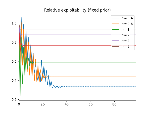
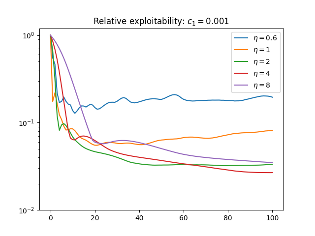
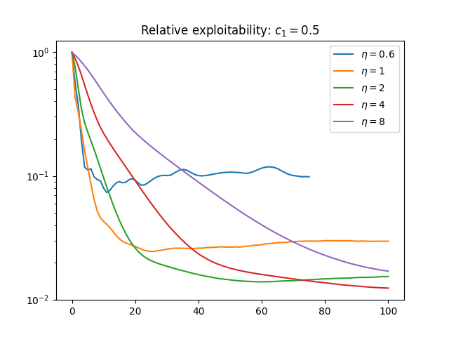
Figure 5.1: Relative exploitability scores. Top: relative exploitability for $c_{1}=0.5$ when applied to a uniform policy as a reference measure, fixed across all iterations. Bottom row: relative exploitability for the prior descent algorithm for two different cost values $c_{1}$.

We adapt in particular the discrete-time version of the SIS model used as test case in [13]. In this model, a virus is assumed to be circulating amongst the population. Each agent can take on two states: susceptible (S), or infected (I). At each moment, the agent can decide to go out (U) or socially distance (D). Thus we have $\mathcal{X}=\{S,I\}$ and $A=\{U,D\}$. The probability of an agent being infected whilst going out is proportional to the fraction of infected people. Once infected, they have a constant probability of recovering at each unit in time. We use the following parameters for the transition kernel:

$$p(S\mid I,U) =p(S\mid I,D)=0.2,$$

$$p(I\mid S,U) =0.9^{2}\cdot\mu_{t}(I),$$

$$p(I\mid S,D) =0.$$

Whilst healthy, there is a cost for socially distancing, and there are larger costs for being infected. As the infection rate in the SIS model does not depend on the proportion of people infected and going out, we adjust the reward to penalise this situation to reflect a desired behaviour of socially distancing whilst infected. Thus, the reward for our numerical example is given by

$$r(S,U)=0,\quad r(S,D)=-0.3,$$

$$r(I,U)=-1.25,\quad r(I,D)=-1.0.$$

In addition to the standard model, we introduce the notion of test result times. Assume that during a pandemic, the population undergoes daily testing in order to determine whether they are infected or not. Here we assume the availability of two testing options, the free option which requires a 3-day turnaround, and a paid option which offers a next-day result. Thus we have for our model

$$\mathcal{D}=\{d_{0}=3,d_{1}=1\},\quad\mathcal{C}=\{c_{0}=0,c_{1}>0\},$$

where we shall consider different values of $c_{1}$ in our numerical experiments.

For the computation of MFNEs for our model, we utilise the mfglib Python package [17]. We incorporate our own script for the mapping $\bm{\nu}\mapsto\bm{\mu}^{\nu}$ so that the existing library can be adapted for our MFG with control of information speed, and in particular to be computed on the augmented space. We first initialise with a uniform policy as the reference measure $q$, and repeatedly apply the mapping $\Psi^{\mathrm{aug}}\circ\Phi^{\mathrm{reg}}_{\eta}$ for a range of values of the regularisation parameter $\eta$. As a benchmark to test for the convergence towards a regularised MFNE, we utilise the exploitability score, which, for a policy $\pi$, is defined by

$$\mbox{Expl}(\pi)\coloneqq\max_{\tilde{\pi}}J_{\Psi^{\mathrm{aug}}(\tilde{\pi})}(\tilde{\pi})-J_{\Psi^{\mathrm{aug}}(\pi)}(\pi).$$

The exploitability score measures the suboptimality gap for a policy $\pi$ when computed with the measure flow induced by the map $\Psi^{\mathrm{aug}}$. An exploitability score is 0 if and only if $\pi$ is an MFNE for the MFG, and a score of $\varepsilon$ indicates that $\pi$ is an $\varepsilon$-MFNE. We refer to the literature such as [19, 31, 27] for a more detailed discussion.

Input : Initial distribution $\bm{\nu}_{0}\in\Delta_{\tilde{\mathcal{Y}}}$, prior policy $q\in\Pi_{DM}$, $tol$

Input : Number of iterations per loop $I$, regularisation parameter $\eta>0$, truncation time $T$.

while $RelExpl>tol$ do

       for $i=0,1,\ldots,I$ do

             for $t=0,1,\ldots,T-1$ do

                   Compute $\bm{\mu}^{\nu}_{t}=(\mu_{t,d})^{d_{0}}_{d=0}\in\Delta^{d_{0}=1}_{\mathcal{X}}$.

                   Compute the regularised $Q$-function $Q^{\mathrm{reg},*}_{\eta,\bm{\nu}}(t,y,u)$ for fixed measures $\bm{\mu}^{\nu}_{t}$.

                   Compute the softmax policy $\pi^{\mathrm{soft}}_{\eta,\bm{\nu},t}=\Phi^{\mathrm{reg}}_{\eta}(\bm{\nu})_{t}$.

                   Compute the induced mean-field $\bm{\nu}_{t+1}=\Psi^{\mathrm{aug}}(\pi^{\mathrm{soft}}_{\eta,\bm{\nu},t})_{t+1}$.

             end for

            

       end for

      $q\leftarrow\pi^{\mathrm{soft}}_{\eta,\bm{\nu}}$.

end while

Algorithm 1 Prior descent for MFG with control of information speed

As the exploitability score in general is dependent on the rewards and the initial policy, we consider instead the relative exploitability, which scales the exploitability score by the initial value. We plot the convergence of the relative exploitability, with the uniform policy as reference measure, fixed across all iterations, in the bottom graph of Figure 5.1. We see that for lower values of $\eta$, the algorithm converges to a lower relative exploitability value. This corresponds to the fact that the regularised MFG with lower values of $\eta$ approximates the unregularised MFG more closely. However, lower values of $\eta$ require a larger number of iterations for convergence. For values of $\eta$ smaller than 0.2, the algorithm does not even converge in our tests and explodes numerically (not plotted in the graph). This demonstrates an inherent limitation of the use of regularisation: one desires a sufficiently high value of $\eta$ in order to guarantee convergence, but high values leads to a convergence to a regularised MFNE that approximates the original problem poorly. Moreover, searching for a suitable value of $\eta$ is computationally expensive.

To mitigate the above issues, we utilise the prior descent algorithm [13]. Here, the reference measure is dynamically updated, by using the policy obtained from the previous iteration as the reference measure for the next iteration. The reference measure can also be updated after a number of iterations instead, creating a double loop for the algorithm. We summarise the prior descent algorithm for the MFG with control of information speed in Algorithm 1. The relative exploitability score is plotted in the top row of Figure 5.1. The score vastly outperforms the case of the fixed prior, and in general, we find that larger values of $\eta$ require more iterations for convergence, but converge to a lower exploitability score. In [13], the prior descent algorithm is further improved by using the heuristic $\eta_{n+1}=\eta_{n}\cdot c$ for some constant $c>1$, gradually increasing the regularisation to aid convergence. We also applied this heuristic for our problem, but for our case we do not see significant differences compared to initialising with large fixed values of $\eta$.

Figure 5.2: Behaviour at MFNE for MCDM-MFG for cost $c_{1}=0.001$.

We now examine the MFNE for the SIS model with testing options for different values of $c_{1}$. Figure 5.2 corresponds to a low cost of $c_{1}=0.001$, whilst Figure 5.3 corresponds to a high cost of $c_{1}=0.05$. We compute the problem up to a terminal time of $T=100$, but the truncate the graphs at $T=75$, as the plots near terminal time are skewed by the artificially imposed terminal condition. The graphs on the right column depicts the behaviour in the choice of testing at equilibrium. The top-right shows the proportion of the population opting for the free test, whilst the bottom-right shows the optimal choice for testing for a healthy individual, given their current testing choice. We see a clear disparity across the two different costs. When the cost of the premium test is low, it is optimal to opt for this regime with probability 0.6, and at equilibrium nearly 80% of the population chooses this option. In comparison, when the cost is high, it is optimal to choose the premium option only about 25% of the time, and less than half of the population use the premium option at equilibrium.

The left columns of Figure 5.2 and Figure 5.3 depict the population behaviour with social distancing, and the proportion of infected at equilibrium. At the beginning, there is a large number of infected people, so it is optimal to socially distance; once the proportion of infected is sufficiently low, a portion of the population starts to go out. This leads to a rebound in infection numbers, so that gradually the population socially distances again, and the cycle repeats. This is depicted by the periodic behaviours in the graph on the left.

Figure 5.3: Behaviour at MFNE for MCDM-MFG for cost $c_{1}=0.05$.

For the case $c_{1}=0.001$, the low cost for premium testing leads to a higher percentage of the population with a more accurate estimation of their status. This leads to larger proportion of people going out, so that the infection occurs at a quicker rate. This in turn then leads to a quick rate of socially distancing, and so forth. This can be seen in the higher frequency of cycles in the infected and distancing graphs of Figure 5.2. Interestingly, as the proportion of infected stabilises as time passes to a similar value, regardless of the cost for the premium testing. The difference lies in the initial periods of peaks and troughs in infected numbers.

Acknowledgements

Jonathan Tam is supported by the EPSRC Centre for Doctoral Training in Mathematics of Random Systems: Analysis, Modelling and Simulation (EP/S023925/1). Collaboration by Dirk Becherer in this project is supported by German Science Foundation DFG through the Berlin-Oxford IRTG 2544, Stochastic Analysis in Interaction.

References

- [1] S. Adlakha, S. Lall, and A. Goldsmith. Information state for Markov decision processes with network delays. In 2008 47th IEEE Conference on Decision and Control, pages 3840–3847. IEEE, 2008.
- [2] S. Adlakha, S. Lall, and A. Goldsmith. Networked Markov decision processes with delays. IEEE Trans. Automat. Control, 57(4):1013–1018, 2011.
- [3] E. Altman and P. Nain. Closed-loop control with delayed information. ACM SIGMETRICS Performance Evaluation Review, 20(1):193–204, 1992.
- [4] B. Anahtarcı, C. Kariksiz, and N. Saldi. Q-learning in regularized mean-field games. Dyn. Games Appl., 13(1):89–117, 2023.
- [5] J. L. Bander and C. White. Markov decision processes with noise-corrupted and delayed state observations. J. Oper. Res. Soc., 50(6):660–668, 1999.
- [6] C. Bellinger, R. Coles, M. Crowley, and I. Tamblyn. Active measure reinforcement learning for observation cost minimization. arXiv:2005.12697, 2020.
- [7] C. Bellinger, A. Drozdyuk, M. Crowley, and I. Tamblyn. Balancing information with observation costs in deep reinforcement learning. In Proceedings of the 35th Canadian Conference on Artificial Intelligence. CAIAC, 2022.
- [8] B. Bruder and H. Pham. Impulse control problem on finite horizon with execution delay. Stochastic Process. Appl., 119(5):1436–1469, 2009.
- [9] P. E. Caines, M. Huang, and R. P. Malhamé. Large population stochastic dynamic games: closed-loop Mckean-Vlasov systems and the Nash certainty equivalence principle. Commun. Inf. Syst., 6(3):221–252, 2006.
- [10] Á. Cartea and L. Sánchez-Betancourt. Optimal execution with stochastic delay. Finance and Stoch., 27(1):1–47, 2023.
- [11] B. Chen, M. Xu, L. Li, and D. Zhao. Delay-aware model-based reinforcement learning for continuous control. Neurocomputing, 450:119–128, 2021.
- [12] C. Cooper and N. Hahi. An optimal stochastic control problem with observation cost. IEEE Trans. Automat. Control, 16(2):185–189, 1971.
- [13] K. Cui and H. Koeppl. Approximately solving mean field games via entropy-regularized deep reinforcement learning. In International Conference on Artificial Intelligence and Statistics, pages 1909–1917. PMLR, 2021.
- [14] M. Geist, B. Scherrer, and O. Pietquin. A theory of regularized Markov decision processes. In International Conference on Machine Learning, pages 2160–2169. PMLR, 2019.
- [15] H.-O. Georgii. Gibbs measures and phase transitions. In Gibbs Measures and Phase Transitions. de Gruyter, 2011.
- [16] N. Guo and V. Kostina. Optimal causal rate-constrained sampling for a class of continuous Markov processes. IEEE Trans. Inform. Theory, 67(12):7876–7890, 2021.
- [17] X. Guo, A. Hu, M. Santamaria, M. Tajrobehkar, and J. Zhang. MFGLib: A library for mean field games. arXiv:2304.08630, 2023.
- [18] X. Guo, A. Hu, R. Xu, and J. Zhang. Learning mean-field games. Adv. Neural. Inf. Process. Syst., 32, 2019.
- [19] X. Guo, A. Hu, and J. Zhang. MF-OMO: An optimization formulation of mean-field games. arXiv preprint arXiv:2206.09608, 2022.
- [20] B. Hajek, K. Mitzel, and S. Yang. Paging and registration in cellular networks: Jointly optimal policies and an iterative algorithm. IEEE Trans. Inform. Theory, 54(2):608–622, 2008.
- [21] O. Hernández-Lerma. Adaptive Markov Control Processes. Applied mathematical sciences. Springer-Verlag, 1989.
- [22] O. Hernández-Lerma and J.-B. Lasserre. Discrete-Time Markov Control Processes. Springer New York, 1996.
- [23] Y. Huang and Q. Zhu. Self-triggered Markov decision processes. In Proc. 60th IEEE CDC, pages 4507–4514, 2021.
- [24] K. Katsikopoulos and S. Engelbrecht. Markov decision processes with delays and asynchronous cost collection. IEEE Trans. Automat. Control, 48(4):568–574, 2003.
- [25] D. Krueger, J. Leike, O. Evans, and J. Salvatier. Active reinforcement learning: Observing rewards at a cost. arXiv:2011.06709, 2020.
- [26] J.-M. Lasry and P.-L. Lions. Mean field games. Jpn. J. Math., 2(1):229–260, 2007.
- [27] M. Laurière, S. Perrin, M. Geist, and O. Pietquin. Learning mean field games: A survey. arXiv:2205.12944, 2022.
- [28] S. Nath, M. Baranwal, and H. Khadilkar. Revisiting State Augmentation Methods for Reinforcement Learning with Stochastic Delays, page 1346–1355. Association for Computing Machinery, New York, NY, USA, 2021.
- [29] A. Nayyar, T. Başar, D. Teneketzis, and V. V. Veeravalli. Optimal strategies for communication and remote estimation with an energy harvesting sensor. IEEE Trans. Automat. Control, 58(9):2246–2260, 2013.
- [30] B. Øksendal and A. Sulem. Optimal stochastic impulse control with delayed reaction. Applied Mathematics and Optimization, 58(2):243–255, 2008.
- [31] J. Pérolat, S. Perrin, R. Elie, M. Laurière, G. Piliouras, M. Geist, K. Tuyls, and O. Pietquin. Scaling mean field games by online mirror descent. page 1028–1037. International Foundation for Autonomous Agents and Multiagent Systems, 2022.
- [32] S. Perrin, J. Pérolat, M. Laurière, M. Geist, R. Elie, and O. Pietquin. Fictitious play for mean field games: Continuous time analysis and applications. Advances in Neural Information Processing Systems, 33:13199–13213, 2020.
- [33] C. Reisinger and J. Tam. Markov decision processes with observation costs: framework and computation with a penalty scheme. arXiv preprint arXiv:2201.07908, 2022.
- [34] N. Saldi, T. Başar, and M. Raginsky. Markov–Nash equilibria in mean-field games with discounted cost. SIAM J. Control Optim., 56(6):4256–4287, 2018.
- [35] N. Saldi, T. Başar, and M. Raginsky. Approximate Nash equilibria in partially observed stochastic games with mean-field interactions. Math. Oper. Res., 44(3):1006–1033, 2019.
- [36] N. Saldi, T. Başar, and M. Raginsky. Partially observed discrete-time risk-sensitive mean field games. Dyn. Games Appl., 13(3):926–960, 2023.
- [37] Y. F. Saporito and J. Zhang. Stochastic control with delayed information and related nonlinear master equation. SIAM J. Control Optim., 57(1):693–717, 2019.
- [38] E. Schuitema, L. Buşoniu, R. Babuška, and P. Jonker. Control delay in reinforcement learning for real-time dynamic systems: A memoryless approach. In 2010 IEEE/RSJ International Conference on Intelligent Robots and Systems, pages 3226–3231. IEEE, 2010.
- [39] V. Tzoumas, L. Carlone, G. J. Pappas, and A. Jadbabaie. LQG control and sensing co-design. IEEE Trans. Automat. Control, 66(4):1468–1483, 2020.
- [40] S. Winkelmann, C. Schütte, and M. v. Kleist. Markov control processes with rare state observation: Theory and application to treatment scheduling in HIV–1. Commun. Math. Sci., 12(5):859–877, 2014.
- [41] W. Wu and A. Arapostathis. Optimal sensor querying: General Markovian and LQG models with controlled observations. IEEE Trans. Automat. Control, 53(6):1392–1405, 2008.
- [42] H. Yoshioka and M. Tsujimura. Analysis and computation of an optimality equation arising in an impulse control problem with discrete and costly observations. J. Comput. Appl. Math., 366:112399, 2020.
- [43] H. Yoshioka, M. Tsujimura, K. Hamagami, and Y. Yoshioka. A hybrid stochastic river environmental restoration modeling with discrete and costly observations. Optimal Control Appl. Methods, 41(6):1964–1994, 2020.
- [44] H. Yoshioka, Y. Yaegashi, M. Tsujimura, and Y. Yoshioka. Cost-efficient monitoring of continuous-time stochastic processes based on discrete observations. Appl. Stoch. Models Bus. Ind., 37(1):113–138, 2021.
- [45] H. Yoshioka, Y. Yoshioka, Y. Yaegashi, T. Tanaka, M. Horinouchi, and F. Aranishi. Analysis and computation of a discrete costly observation model for growth estimation and management of biological resources. Comput. Math. Appl., 79(4):1072–1093, 2020.