Particle-hole asymmetric ferromagnetism and spin textures in the triangular Hubbard-Hofstadter model

Abstract

In a lattice model subject to a perpendicular magnetic field, when the lattice constant is comparable to the magnetic length, one enters the “Hofstadter regime,” where continuum Landau levels become fractal magnetic Bloch bands. Strong mixing between bands alters the nature of the resulting quantum phases compared to the continuum limit; lattice potential, magnetic field, and Coulomb interaction must be treated on equal footing. Using determinant quantum Monte Carlo (DQMC) and density matrix renormalization group (DMRG) techniques, we study this regime numerically in the context of the Hubbard-Hofstadter model on a triangular lattice. In the field-filling phase diagram, we find a broad wedge-shaped region of ferromagnetic ground states for filling factor $\nu\lesssim 1$, bounded by incompressible states at filling factor $\nu=1$. For magnetic field strengths $\Phi/\Phi_{0}\lesssim 0.4$, we observe signatures of SU(2) quantum Hall ferromagnetism in the lowest magnetic Bloch band; however, we find no numerical evidence for conventional quantum Hall skyrmions. At large fields $\Phi/\Phi_{0}\gtrsim 0.4$, above the ferromagnetic wedge, we observe a low-spin metallic region with spin correlations peaked at small momenta. We argue that the phenomenology of this region likely results from exchange interaction mixing fractal Hofstadter subbands. The phase diagram derived beyond the continuum limit points to a rich landscape to explore interaction effects in magnetic Bloch bands.

I Introduction

Landau levels are paradigmatic examples of topological flat bands. They arise from a simple continuum model of a two-dimensional electron gas under the influence of an out-of-plane orbital magnetic field, and have been instrumental in explaining a wide variety of quantum Hall phenomena [1]. The effectiveness of the Landau level picture relies on two key assumptions. First, lattice effects are neglected: all Landau levels are flat, have uniform quantum geometry, continuous magnetic translation symmetry, and continuous rotational symmetry. Second, the Landau level spacing, $h\omega_{c}$, is typically assumed to be the largest energy scale in the problem of interest. Any fully filled and empty bands are inert, so the many-body problem of interacting electrons only needs to be treated within one isolated Landau level. The lowest Landau level, in particular, satisfies a number of desirable analytical properties [2, 3], some of which have one-to-one correspondence in ideal Chern bands [4, 5, 6, 7].

While the Landau level picture works well for systems with magnetic length much greater than the lattice constant, including GaAs and monolayer graphene, such a description breaks down in moiré materials, whose lattice constants are comparable with magnetic length at moderate magnetic fields. Within this “Hofstadter regime,” Landau levels become fractal magnetic Bloch bands [8, 9] and acquire nonzero dispersion, non-uniform Berry curvature, and discrete magnetic translation symmetry [10, 11]. It is natural to ask at this point if results obtained using the continuum model persist or generalize appropriately in the strong lattice limit. Conversely, the lattice potential may precipitate new phases of matter that cannot be captured in the continuum model. Recent works along this line have focused on the lattice fractional quantum Hall effect [12, 13] and fractional Chern insulators [14, 15] which may [16, 17] or may not [18, 19, 20, 21] be adiabatically connected to the continuum limit.

Another phenomenon of interest is quantum Hall ferromagnetism (QHFM) and associated skyrmions [22]. The mathematical description of QHFM has been generalized to a large variety of multicomponent topological flat bands, under the moniker of generalized/flavor/isospin QHFM, or flavor polarization of Chern bands. In moiré materials, particularly magic-angle twisted bilayer graphene, correlated insulating states at integer Chern numbers [23, 24, 25, 26, 27, 28, 29, 30] are abundant, and $\nu=\pm 2$ gaps have been identified to host skyrmion excitations [31]. Theoretical proposals suggest that skyrmions exist in flat Chern bands, and may even contribute to superconductivity [32, 33, 34, 35].

In the standard picture for SU(2) QHFM [22, 36, 37], each Landau level with $N_{\phi}$ degenerate single-particle orbitals can accommodate $2N_{\phi}$ electrons with an internal SU(2) spin degree of freedom. Landau level filling factor $\nu=1$ corresponds to $N_{\uparrow}+N_{\downarrow}=N_{\phi}$, i.e. half-filling the lowest Landau level. Coulomb repulsion between electrons induces a ferromagnetic exchange interaction, $E_{\mathrm{X}}$, so the $\nu=1$ ground state is spin polarized with total spin quantum number $S=N_{\phi}/2$, even in the absence of Zeeman splitting. The lowest energy-charged excitations about the $\nu=1$ quantum Hall ferromagnet are not bare particles and holes, but charge-spin texture bound states known as skyrmions. The existence of quantum Hall skyrmions manifests experimentally as rapid depolarization: doping slightly away from $\nu=1$ dramatically reduces the total spin $S$, as each addition and removal of one unit of charge is associated with a large number of spin flips [38, 39, 40]. While ferromagnetic insulating states also occur in higher Landau levels at odd integer filling factors $\nu=3,5,7...$, bare particles and holes, rather than skyrmions, are believed to be the lowest charged quasiparticle excitations in higher Landau levels [41, 42, 43]. Additionally, Landau level mixing is thought to destabilize $\nu=1$ skyrmions [44, 45]. The conditions for skyrmion stability in general Chern bands remains an open question [46, 47, 48].

In order to explore possible phases in interacting lattice quantum Hall systems, and explore the question of skyrmion stability, we use two numerically exact and unbiased methods, determinant quantum Monte Carlo (DQMC) [49, 50] and density matrix renormalization group (DMRG)[51, 52, 53, 54], to study the Hubbard-Hofstadter (HH) model on a triangular lattice. By using unbiased numerical methods, we are able to address the analytically intractable regime of non-flat, non-isolated bands. The HH model is a minimal lattice Hamiltonian which incorporates the effects of a strong orbital magnetic field and on-site electron repulsion. It is a versatile model that has been studied in the context of topological superconductivity [55, 56], and may be used as a building block to create a time-reversal-symmetric variant [57, 58]. We expect that the HH model can be realized in cold-atom quantum simulators [59, 60, 61, 62] in an artificial gauge field [63].

The HH model has recently been studied in the square and hexagonal lattice geometry via DQMC [64, 65] and in the square geometry via DMRG [66]. Our results for the triangular lattice reveal a large ferromagnetic wedge for $\nu\lesssim 1$ which evolves into an incompressible quantum Hall ferromagnet at $\nu=1$, and singlet ground states everywhere else, broadly consistent with prior work [66, 65]. This agreement strongly suggests that these features of the HH model are lattice-geometry independent. In addition to corroborating prior work, we also show that whether the $\nu=1$ QHFM state extends to the high field limit $\Phi/\Phi_{0}=0.5$ depends on the competition of the exchange interaction and an intervening small Chern band gap carrying Chern number $-4$. While we do not observe signatures of conventional quantum Hall skyrmions upon doping slightly away from $\nu=1$, we uncover a region of parameter space above the ferromagnetic wedge that is low-spin, metallic, and exhibits spin correlations peaked at small momenta. We propose that this region is a spin-textured metal precipitated by competition between tendency towards singlet and spin-polarized ground states, and indicate directions for future study. Our work complements recent analytical studies [47, 48] and is generally relevant for understanding the behavior of strongly correlated electrons under large magnetic fields.

II Methods

We study the single-band Hubbard-Hofstadter model

$$H=-\sum_{ij\sigma}t_{ij}\left\{\exp\left[\mathrm{i}\varphi_{ij}\right]c_{i\sigma}^{\dagger}c_{j\sigma}+\mathrm{h.c.}\right\}-\mu\sum_{i\sigma}n_{i\sigma}\\ +U\sum_{i}\left(n_{i\uparrow}-1/2\right)\left(n_{i\downarrow}-1/2\right),$$ (1)

on a two-dimensional triangular lattice. The hopping integral $t_{ij}=t$ between nearest neighbor sites $\langle ij\rangle$, and $t_{ij}=0$ otherwise, $\mu$ is the chemical potential, and $U$ is the on-site Coulomb interaction strength. $c_{i\sigma}^{\dagger}$ ($c_{i\sigma}$) is the creation (annihilation) operator for an electron on site $i$ with spin $\sigma\in\{\uparrow,\downarrow\}$, and $n_{i\sigma}=c_{i\sigma}^{\dagger}c_{i\sigma}$ measures the number of electrons of spin $\sigma$ on site $i$. A spatially uniform and static orbital magnetic field is introduced by the Peierls substitution via the phase

$$\varphi_{ij}=\dfrac{2\pi}{\Phi_{0}}\int_{\mathbf{r}_{i}}^{\mathbf{r}_{j}}\mathbf{A}\cdot d\bm{\ell},$$ (2)

where $\Phi_{0}=h/e$ is the magnetic flux quantum, and $\mathbf{r}_{i}=(r_{ix},r_{iy})$ is the position of site $i$, and the path integral is taken along the shortest straight line path between sites $i$ and $j$. The vector potential $\mathbf{A}$ generates out-of-plane magnetic field $\mathbf{B}=B\mathbf{\hat{z}}$, and has gauge freedom parametrized by $\alpha\in\mathbb{R}$:

$$\mathbf{A}(\mathbf{r})=B\begin{bmatrix}-\alpha r_{y}\\ (1-\alpha)r_{x}\end{bmatrix}.$$ (3)

In this work we use $\alpha=1/2$, which corresponds to the symmetric gauge $\mathbf{A}(\mathbf{r})=B(-r_{y}\mathbf{\hat{x}}+r_{x}\mathbf{\hat{y}})/2$. We have verified that the results reported in this work do not depend on the choice of gauge. Zeeman coupling is neglected. While the Hamiltonian breaks time-reversal, parity, and particle-hole symmetries, it preserves the SU(2) spin symmetry. This choice is consistent with the energy hierarchy $E_{\mathrm{Z}}\ll E_{\mathrm{X}}$ (where $E_{\mathrm{Z}}=g\mu_{B}B$ is Zeeman splitting) required to observe quantum Hall skyrmions.

The Hamiltonian in Eq. 1 is simulated on a finite cluster with lattice constant $a$, and $N_{1}$ and $N_{2}$ sites respectively, along the directions $\mathbf{a}_{1}=a(1/2,\sqrt{3}/2)$, $\mathbf{a}_{2}=a(-1/2,\sqrt{3}/2)$, which are the primitive lattice vectors of the triangular lattice. $N=N_{1}N_{2}$ denotes the total number of sites. Modified periodic boundary conditions are implemented, consistent with magnetic translation symmetry [67, 11], as described in detail in Appendix A. Requiring that the wave function be single-valued on the torus gives the flux quantization condition $\Phi/\Phi_{0}=N_{\phi}/N$, where $\Phi=\sqrt{3}Ba^{2}/2$ is the magnetic flux threading each unit cell and $N_{\phi}$ is an integer. Denoting the number of electrons in the system as $N_{e}=N_{\uparrow}+N_{\downarrow}$, filling factor $\nu=1$ corresponds to $N_{e}=N_{\phi}$. Electron number density $n=N_{e}/N\in[0,2]$.

Throughout this text, magnetic field strengths are denoted in units of $\Phi/\Phi_{0}$ and the lattice constant is set to $a=1$. Following Ref. [68], the terms “magnetic Bloch band,” “Hofstadter band,” and “Chern band” are used interchangeably. We use $n=C(\Phi/\Phi_{0})+s$ to parametrize non-interacting gaps and correlated states in $(n,\Phi/\Phi_{0})$ parameter space. Matching the notation used in existing literature, when $s=0$, we denote $C$ by $\nu$.

DQMC simulations of Eq. 1 are performed on clusters with linear size $N_{1}=N_{2}=6,8,9,$ and $12$. As shown in Appendix D, finite-size effects in DQMC data at accessible temperatures are minimal, so we may safely take DQMC results to be representative of the thermodynamic limit. Error bars in DQMC results, when shown, denote $\pm 1$ standard error of the mean, estimated by jackknife resampling. Detailed DQMC simulation parameters are listed in Appendix B, and fermion sign for a typical set of parameters is shown in Appendix C.

DMRG simulations are performed using the ITensor library [69, 70]. We keep bond dimensions up to 2000 to get quasi-exact results, with truncation error of order $10^{-6}$ or below. In order to compare with DQMC results directly, we present DMRG calculations on the same torus geometry with periodic boundary conditions in both directions. Due to the rapid growth of entanglement with system size in the torus geometry, DMRG calculations are limited to clusters with $N_{1}=6$ and $N_{2}=3$.

III Summary of Key Findings

In this work we primarily investigate the $n\in[0,0.5]$, $\Phi/\Phi_{0}\in[0,0.5]$ corner of parameter space, which encompasses the lowest several Chern bands, and approaches the continuum limit as $n\rightarrow 0$, $\Phi/\Phi_{0}\rightarrow 0$. Our main results can be summarized in a schematic phase diagram shown in  Fig. 1. We first highlight the primary findings and then elaborate on these observations.

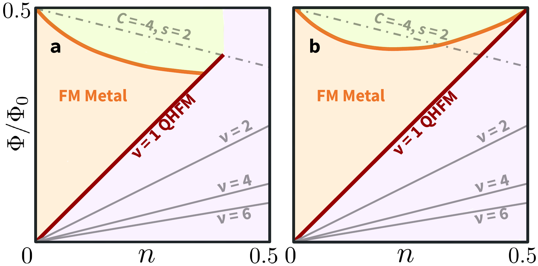
Figure 1: Phase diagram sketches of Hubbard-Hofstadter model on a triangular lattice for a $U/t\lesssim 4$ and b $U/t\gtrsim 8$ in the $n\in[0,0.5]$, $\Phi/\Phi_{0}\in[0,0.5]$ quadrant of $(n,\Phi/\Phi_{0})$ parameter space. Dot-dashed grey lines denote the Chern band gap satisfying the Diophantine equation $n=C(\Phi/\Phi_{0})+s$ ($C=-4,s=2$) [9]. Solid grey lines denote even integer Chern band gaps as annotated (the intercept $s=0$ implicitly, so that $C=\nu$). Pale purple shadings indicate metallic states with short-range antiferromagnetic correlations. Pale green shading indicates anomalous metal with small-$q$ spin correlations.

In a triangular-shaped wedge of parameter space bounded below by $\nu\lesssim 1$, the ground state is ferromagnetic and metallic, only becoming incompressible at $\nu=1$. We call this $\nu\lesssim 1$ region the “FM wedge,” and identify the incompressible state at $\nu=1$ as the lattice realization of $\nu=1$ QHFM. Outside the FM wedge, except for incompressible states at filling factors $\nu=2,4,6$, the ground state is metallic with short-range antiferromagnetic fluctuations, exhibiting behavior largely consistent with weakly interacting bands. For $U/t\lesssim 4$ in Fig. 1a, QHFM terminates below $(n,\Phi/\Phi_{0})=(0.4,0.4)$, and the FM wedge is bounded above by the straight line $n=-4(\Phi/\Phi_{0})+2$. for $U/t\gtrsim 8$ in Fig. 1b, QHFM extends to the highest field strength $\Phi/\Phi_{0}=0.5$. No conventional skyrmion signatures are observed in the vicinity of $\nu=1$, contrary to expectations from the continuum limit.

Nontrivial spin features are observed above the FM wedge, for $\Phi/\Phi_{0}\gtrsim 0.4$. In this region, the ground state is metallic and low-spin. At finite temperatures, the equal-time spin correlations are peaked at small momenta, different from both nearby ferromagnetic order and the non-interacting Lindhard susceptibility. We suggest that this region hosts a novel spin-textured metallic phase due to the competition between the exchange interaction and Hofstadter subband gaps.

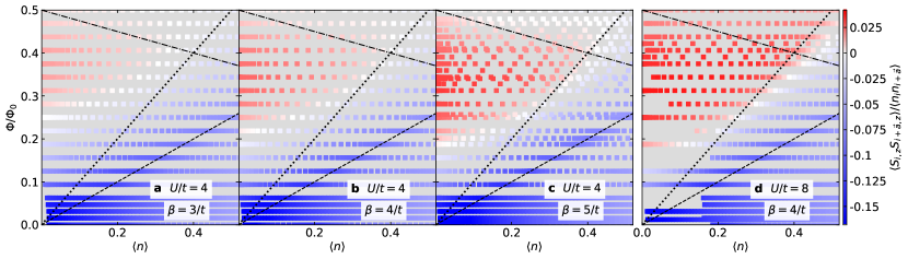
Figure 2: Equal-time nearest-neighbor spin correlation normalized by nearest-neighbor charge correlation, $\langle S_{i,z}S_{i+\mathbf{a},z}\rangle/\langle n_{i}n_{i+\mathbf{a}}\rangle$, obtained by DQMC. This normalization convention was chosen to ensure that we are not simply observing higher spin correlation values due to higher particle density. a-c show temperature dependence at fixed $U/t=4$; b and d show Hubbard $U$ dependence at fixed inverse temperature $\beta=4/t$. Dotted lines denote $\nu=1$, dashed lines denote $\nu=2$, and dot-dashed lines denote $n=-4(\Phi/\Phi_{0})+2$. The colorbar is saturated in the minimum direction. DQMC data combine results obtained on clusters of size $8\times 8$, $9\times 9$ and $12\times 12$, an appropriate procedure since finite size effects are small for this local observable, as shown in Appendix D.

IV Results and Discussion

Finite temperature DQMC data for nearest-neighbor spin correlations $\langle S_{i,z}S_{i+\mathbf{a},z}\rangle$, normalized by nearest-neighbor particle density correlations $\langle n_{i}n_{i+\mathbf{a}}\rangle$, shown in Fig. 2, reveal a triangular wedge of ferromagnetic correlations at $\nu\lesssim 1$, and antiferromagnetic correlations for $\nu\gtrsim 1$. Fig. 2a-c show for fixed $U/t=4$, local ferromagnetic correlations in the $\nu\lesssim 1$ region become stronger as temperature decreases. Yet, the region of ferromagnetic correlations is roughly bounded above by the straight line $n=-4(\Phi/\Phi_{0})+2$, down to the lowest accessible temperatures (see Fig. 13 for extended temperature dependence). This is in direct contrast to the $U/t=8$ case shown in Fig. 2d, where ferromagnetic correlations persist to largest field $\Phi/\Phi_{0}=0.5$ (see Fig. 14 for extended interaction dependence). The $n=-4(\Phi/\Phi_{0})+2$ line corresponds to a small non-interacting Chern band gap (see dot-dashed line in Fig. 8) and intersects with the $\nu=1$ line at $(n,\Phi/\Phi_{0})=(0.4,0.4)$. In the absence of interactions, states on this line represent singlet ground states. It is therefore a natural boundary for the termination of ferromagnetism. The qualitatively different behavior of $U/t=4$ and $U/t=8$ suggests that the latter corresponds to sufficiently high interaction strength that the induced exchange splitting is larger than the non-interacting Chern band gap, allowing ferromagnetism to penetrate to $\Phi/\Phi_{0}=0.5$.

Zero-temperature DMRG simulations indicating the ground state spin degeneracy, shown in Fig. 3a-b, support the findings of DQMC. Triangular wedges of maximally spin polarized ground states at $\nu\lesssim 1$ match well with regions of ferromagnetic correlations in the DQMC results. Singlet configurations are preferred at $\nu>1$, which is also consistent with short-range antiferromagnetic correlations found by DQMC. As $\Phi/\Phi_{0}\rightarrow 0$, $n\rightarrow 0$, energy scales are compressed and become smaller than temperatures accessible via DQMC. Together, Fig. 2 and Fig. 3a-b demonstrate the shape and extent of the FM wedge.

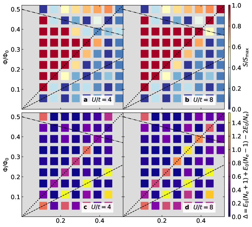
Figure 3: DMRG ground state spin degeneracy (top row) and charge gap (bottom row). a-b Spin degeneracies are plotted as $S/S_{\mathrm{max}}$, where $S_{\mathrm{max}}=N_{e}/2$. States differing in energy by less than $10^{-4}t$ are treated as degenerate. Red color indicates that the ground state is maximally spin polarized in its particle sector, while blue color indicates that the ground state is a singlet configuration. c-d Charge addition-removal gap, $\Delta(N_{e})$ as defined in Eq. 4. DMRG data are obtained on $3\times 6$ cluster. The colorbar in c-d are saturated in the maximum direction in order to improve the visibility of the $\nu=1$ gaps.

Incompressible states along $\nu=1$ and $\nu=2$ observed in Refs. [66, 65] are examined by calculating the particle addition-removal gap

$$\Delta(N_{e})=E_{0}(N_{e}+1)+E_{0}(N_{e}-1)-2E_{0}(N_{e}),$$ (4)

where $E_{0}(N_{e})$ denotes the ground state energy in the $N_{e}$-electron sector. $\Delta(N_{e})$ obtained by DMRG are shown in Fig. 3c for $U/t=4$ and Fig. 3d for $U/t=8$. The charge gap along $\nu=2$ is robust against $U$, showing that this Chern band gap is not closed by the Hubbard interaction at these interaction strengths [64]. Along $\nu=1$, a secondary gap emerges. It is larger for higher Hubbard $U$, with a maximum gap value of $\Delta=1.5t$ for $U/t=8$ on the $3\times 6$ cluster (for comparison with DQMC results, see Appendix F). Along $\nu=1$, the charge gap is greatly reduced above $\Phi/\Phi_{0}\sim 0.4$ for $U/t=4$, while it persists to higher field strengths, near $\Phi/\Phi_{0}\sim 0.5$, for $U/t=8$, which matches the extent of ferromagnetic ground states observed in Fig. 3a-b. Incompressibility and ferromagnetism are concomitant along the $\nu=1$ line up to the intersection with the $C=-4$ line, consistent with a $\nu=1$ lattice QHFM. Above the interaction, a critical Hubbard $U$ strength is required for the QHFM to extend to maximum field.

Given evidence for the $\nu=1$ QHFM in the HH model, it is natural to seek evidence for skyrmionic ground states near $\nu=1$, as predicted in the continuum limit. However, our data do not show signatures for standard quantum Hall skyrmions near $\nu=1$ when $\Phi/\Phi_{0}\lesssim 0.4$. Fig. 3a-b show that the ground state upon removing one electron from $\nu=1$ ($N_{e}=N_{\phi}-1$) has $S=N_{e}/2$. The ground state upon adding one electron to $\nu=1$ ($N_{e}=N_{\phi}+1$) has $S=(N_{e}-2)/1$. These spin numbers are consistent with bare electrons and holes, rather than skyrmions, being the favored charge excitations [39]. These results are inconsistent with Ref. [66], which suggests that slightly electron doping the $\nu=1$ QHFM may produce a narrow strip of skyrmion ground states. This discrepancy may be explained by two possible considerations. In DMRG simulations, a $3\times 6$ cluster cannot access the $\nu\rightarrow 1^{+}$ region to observe spin texture seen in Ref. [66]. In DQMC simulations, accessible temperatures may be much larger than the skyrmion excitation gap (if one exists), which will smear out any spin texture.

However, we emphasize that there is no fundamental reason that a quantum Hall ferromagnet must be accompanied by skyrmions, as evidenced by the $\nu=3,5,7...$ QHFM states which have bare particles and holes as the lowest charged excitations. As the question of skyrmion stability is a purely energetic one, it is possible that band geometry or dispersion reduces skyrmion stability, although how this occurs and to what extent is not clear a priori. Additionally, while a sufficiently strong, purely local interaction ($\delta$-function potential in the continuum model, Hubbard interaction in this lattice model) is sufficient to generate ferromagnetic exchange, and thereby induce a quantum Hall ferromagnet, longer-range repulsive interactions may be required for skyrmions to be the lowest energy quasiparticle near the $\nu=1$ QHFM. This was discussed in the Landau level picture in Refs. [71, 72], but requires further study in the lattice context [73, 74].

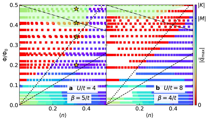
Figure 4: Distance of peak position of $\chi_{s}(\mathbf{q},\tau=0)$ (Eq. 30) to $\Gamma$, denoted by $|q_{\mathrm{max}}|$. Angular information is suppressed and only distance to $\Gamma$ is shown. a inverse temperature $\beta=5/t$, Hubbard interaction $U/t=4$ and b inverse temperature $\beta=4/t$, Hubbard interaction $U/t=8$. Red color indicates ferromagnet correlations, while blue-purple colors indicate antiferromagnetic correlations peaked at large momentum. In the $\nu<1$ region above the ferromagnetic wedge, spin correlations are peaked at small momentum $\lvert\mathbf{q}_{\mathrm{max}}\rvert\leq\lvert\mathbf{K}\rvert/2$. Yellow stars mark four representative points analyzed in Fig. 5. DQMC data combine results obtained on clusters of size $8\times 8$, $9\times 9$, and $12\times 12$.

We next discuss in more detail the high-field region indicated by pale green shading in Fig. 1. We identify its boundary using the peak position of spin correlations in momentum space; these DQMC results are shown in Fig. 4 (see Fig. 15 for extended interaction dependence). For both $U/t=4$ and $U/t=8$, the $\nu>1$ region is dominated by short-range antiferromagnetic correlations peaked at momentum $\mathbf{K}$ (purple) or $\mathbf{M}$ (blue), which are high symmetry points in the triangular lattice Brillouin Zone. For $\nu\lesssim 1$, spin correlations are peaked at $\Gamma$. This region is smaller for $U/t=4$ than for $U/t=8$, which is also consistent with our findings based on Fig. 2 and Fig. 3. Above the FM wedge, the peak at $\Gamma$ gives way to peaks at small momenta with $\lvert\mathbf{q}\rvert\leq\lvert\mathbf{K}\rvert/2$ (green, top of Fig. 4). DMRG calculations (Fig. 3) indicate this region has low-spin ground states and no charge gap. For $U/t=4$ in Fig. 4a, as particle density increases to $\langle n\rangle\sim 0.4$, the small-$q$ spin correlations abruptly transition to correlations peaked at $\mathbf{K}$. For $U/t=8$ in Fig. 4b, as particle density increases, the small-$q$ spin correlations first transition to ferromagnetic correlations near $\nu=1$ then to antiferromagnetic correlations peaked at $\mathbf{K}$ for $\nu>1$. By comparison, the non-interacting Lindhard susceptibility is peaked near $\mathbf{K}$ in the entire $n\in[0,0.5]$, $\Phi/\Phi_{0}\in[0,0.5]$ parameter space quadrant.

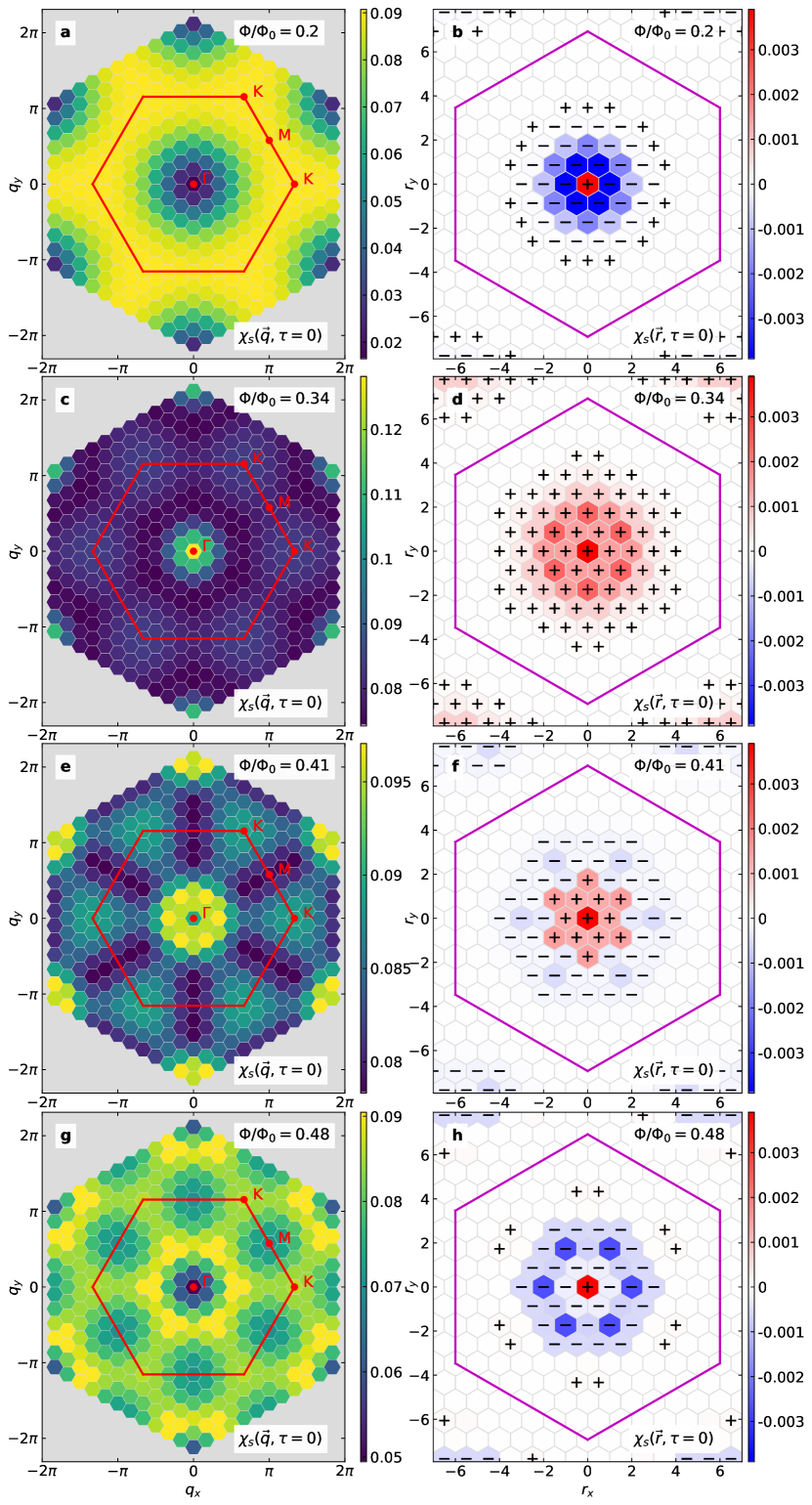
Figure 5: Equal-time spin correlation for four representative points marked by stars in Fig. 4. Each row represents a different field strength. All plots have fixed inverse temperature $\beta=6/t$, Hubbard interaction $U/t=4$, and particle density $\langle n\rangle=0.34$. Each row shows a different field strength, and field strength increases as we move down the plot. The first column (a,c,e,g) shows momentum-space spin correlations $\chi_{s}(\mathbf{q},\tau=0)$(Eq. 30). The second column (b,d,f,h) shows the corresponding real-space spin correlations $\chi_{s}(\mathbf{r},\tau=0)$(Eq. 29). In real-space plots, data points annotated with a $+$ or $-$ sign are nonzero by at least two standard errors, and color bars are saturated in both directions in order to improve contrast. DQMC data are obtained on $12\times 12$ cluster.

To further examine the anomalous spin correlations above the FM wedge, we choose four representative points in parameter space (marked by stars in Fig. 4a) which have identical particle density and increasing magnetic field strength. Their equal-time spin correlations in both real and momentum space, shown in Fig. 5, demonstrate the dramatic evolution of spin correlations in different phases as field strength increases. For the sake of comparison, the non-interacting Lindhard responses at identical $(n,\Phi/\Phi_{0})$ points are shown in Fig. 9. The point $(n,\Phi/\Phi_{0})=(0.34,0.2)$ (shown in Fig. 5a-b) lies in the $\nu>1$ low-spin metallic region. It exhibits short-range antiferromagnetic correlations with broad peaks centered at $\mathbf{K}$. The profile of spin correlations in Fig. 5a matches the non-interacting Lindhard susceptibility in Fig. 9a closely, indicating that the $\nu>1$ area is weakly interacting. The point $(n,\Phi/\Phi_{0})=(0.34,0.34)$ (shown in Fig. 5c-d) lies on the $\nu=1$ QHFM line. It exhibits ferromagnetic correlations peaked at $\Gamma$, which is consistent with a ferromagnetic ground state. The spin correlations are (unsurprisingly) different from the non-interacting case, Fig. 9c, indicating the strong influence of interactions in the FM wedge.

The point $(n,\Phi/\Phi_{0})=(0.34,0.41)$ (shown in Fig. 5e-f) lies on the crossover between the FM wedge and the high-field metallic state. It exhibits weak spin correlations peaked at $\mathbf{q}\sim\mathbf{K}/4$, and the local ferromagnetic correlations give way to antiferromagnetic correlations at larger distances. These spin correlations are reminiscent of the triple-$q$ structures commonly reported in magnetic skyrmion literature [75], but because this region does not hug the $\nu=1$ QHFM, these spin correlation features should not be interpreted as signatures of standard quantum Hall skyrmions. Above the crossover, $(n,\Phi/\Phi_{0})=(0.34,0.48)$ (shown in Fig. 5g-h) exhibits stronger momentum space spin correlations peaked at $\mathbf{q}\sim\mathbf{K}/3$ and oscillatory real space correlations. While it is unclear if the regions shown in Fig. 5e-f and Fig. 5g-h belong to distinct phases, the results are different from both the neighboring FM wedge and the Lindhard susceptibility, shown in Fig. 9e-h. As the spin susceptibility peaks shown in Fig. 5e and g stay at the same position over a broad range of particle density (green shading near the top of Fig. 4), an description in terms of “fluctuating stripes” is also inappropriate.

Below we discuss considerations relevant to interpreting the high-field metal with small-$q$ spin fluctuations. In the ground state of the non-interacting Hofstadter model, in the high-field regime, the lowest Chern band splits into a fractal sequence of sub-bands and sub-band gaps with Chern number $-4,-8,-12,...$, as shown in Fig. 8. While the $C=-4$ gap is the largest of the subband gaps, its size is still small ($\approx 0.2t$), so no signature of $C=-4$ (and any higher Chern number sub-bands) is observed in the finite temperature charge compressibility, as shown in Figs. 10 and 11. However, because fully filled Chern bands must have a singlet ground state, the high-field fine structure of the lowest Chern band necessarily suppresses ferromagnetic order and forms a natural upper bound for the FM wedge. Above the FM wedge, the Coulomb exchange interaction is comparable to the fractal Chern band bandwidths and band gaps, and Landau level mixing effects are strong. The competition between tendencies toward singlet and spin-polarized ground states may enable the formation of a spin-textured metal. As the Hofstadter subbands with $\Phi/\Phi_{0}\rightarrow 0.5$ are under strong lattice influence, this particular region is a rich breeding ground for quantum fluids with no counterpart in the continuum [76]. Our results thus highlight a parameter region that warrants further scrutiny.

V Conclusions

In this work, we numerically study the Hubbard-Hofstadter model on a triangular lattice using DQMC and DMRG. We observe a large ferromagnetic wedge for $\nu\lesssim 1$ and a quantum Hall ferromagnet at $\nu=1$ which is not accompanied by signatures of conventional quantum Hall skyrmions, and singlet ground states elsewhere. We find that when the Hubbard interaction $U$ is small, ferromagnetism is bounded above by the $n=-4(\Phi/\Phi_{0})+2$ Chern band gap, whereas a sufficiently large Hubbard $U$ allows ferromagnetism to exceed this natural boundary. Finally, we identify a region of parameter space above the ferromagnetic wedge, exhibiting small-$q$ spin fluctuations and competition of energy scales. Interactions in this high magnetic field limit may drive a reorganization of finely spaced Chern bands to heretofore unstudied metallic states with spin texture but no magnetic order [77].

Our study shows that unbiased numerical methods applied to interacting lattice Chern bands may lead to results that are dramatically different from expectations based on the continuum limit and uncover fundamentally new physics. We expect the confluence of lattice potential, magnetic field, and interactions to produce novel states at a wide range of particle densities, particularly as half-filling is approached and strong correlations dominate the complex insulating phases nearby [78].

VI Data and Code Availability

Aggregated numerical data and analysis routines required to reproduce the figures can be found at 10.5281/zenodo.8339843. Raw simulation data that support the findings of this study are stored on the Sherlock cluster at Stanford University and are available from the corresponding author upon reasonable request.

The most up-to-date version of our DQMC simulation code can be accessed at https://github.com/katherineding/dqmc-dev.

VII Acknowledgements

We are especially thankful for insightful comments and invaluable suggestions by Steve Kivelson, Shivaji Sondhi, Andrei Bernevig, Hongchen Jiang, Junkai Dong and Nishchhal Verma. We are also indebted to helpful discussions with Sankar Das Sarma, Arno Kampf, Xiaoliang Qi, Donna Sheng, Emily Zhang, Jiachen Yu, Kyung-Su Kim, Paul Neves, Tomohiro Soejima, Patrick Ledwith, Daniel Parker, Vedant Dhruv, Vladimir Calvera, and Chaitanya Murthy.

This work was supported by the Center for Quantum Sensing and Quantum Materials, a DOE Energy Frontier Research Center, grant DE-SC0021238 (JKD, PM, PWP, BEF, and TPD). Portions of this work (LY, WOW, BM) were supported by U.S. Department of Energy (DOE), Office of Basic Energy Sciences, Division of Materials Sciences and Engineering. ZZ was supported by a Stanford Science fellowship. CP acknowledges the support of the U.S. Department of Energy, Office of Science, Basic Energy Sciences under Award No. DE-SC0022216. EWH was supported by the Gordon and Betty Moore Foundation’s EPiQS Initiative through grants GBMF 4305 and GBMF 8691. Computational work was performed on the Sherlock cluster at Stanford University and on resources of the National Energy Research Scientific Computing Center, supported by the U.S. DOE, Office of Science, under Contract no. DE-AC02-05CH11231.

Appendix A Boundary conditions

As mentioned in the main text, the real space primitive lattice vectors of the triangular lattice is

$$\mathbf{a}_{1}=\frac{a}{2}\begin{bmatrix}1\\ \sqrt{3}\end{bmatrix},\quad\mathbf{a}_{2}=\frac{a}{2}\begin{bmatrix}-1\\ \sqrt{3}\end{bmatrix}.$$ (5)

Each lattice site has 6 nearest neighbors located at $\pm\mathbf{a}_{1,2,3}$, where $\mathbf{a}_{3}=(a,0)$.

Lattice sites indexed by $i=(i_{1},i_{2})$ and $j=(j_{1},j_{2})$ have spatial positions

$$\mathbf{r}_{i} =i_{1}\mathbf{a}_{1}+i_{2}\mathbf{a}_{2}=\frac{i_{1}}{2}\begin{bmatrix}1\\ \sqrt{3}\end{bmatrix}+\frac{i_{2}}{2}\begin{bmatrix}-1\\ \sqrt{3}\end{bmatrix}$$

$$=\begin{bmatrix}\dfrac{1}{2}(i_{1}-i_{2})\\ \dfrac{\sqrt{3}}{2}(i_{1}+i_{2})\end{bmatrix}=\begin{bmatrix}r_{ix}\\ r_{iy}\end{bmatrix},$$ (6)

$$\mathbf{r}_{j} =j_{1}\mathbf{a}_{1}+j_{2}\mathbf{a}_{2}$$

$$=\begin{bmatrix}\dfrac{1}{2}(j_{1}-j_{2})\\ \dfrac{\sqrt{3}}{2}(j_{1}+j_{2})\end{bmatrix}=\begin{bmatrix}r_{jx}\\ r_{jy}\end{bmatrix}.$$ (7)

The midpoint between site $i$ and site $j$ has position

$$\mathbf{r}_{m}(i,j)=\frac{1}{2}(\mathbf{r}_{i}+\mathbf{r}_{j})=\frac{1}{2}\begin{bmatrix}r_{ix}+r_{jx}\\ r_{iy}+r_{jy}\end{bmatrix}\\ =\frac{1}{4}\begin{bmatrix}j_{1}-j_{2}+i_{1}-i_{2}\\ \sqrt{3}(j_{1}+j_{2}+i_{1}+i_{2})\end{bmatrix}=\begin{bmatrix}r_{mx}\\ r_{my}\end{bmatrix}.$$ (8)

The difference between site $i$ and site $j$, indexed by $\Delta=j-i=(d_{1},d_{2})$, for integration path $\mathbf{r}_{i}\rightarrow\mathbf{r}_{j}$, corresponds to a position change of

$$\mathbf{r}_{\Delta}(i,j) =\mathbf{r}_{j}-\mathbf{r}_{i}=\begin{bmatrix}r_{jx}-r_{ix}\\ r_{jy}-r_{iy}\end{bmatrix}$$

$$=\begin{bmatrix}\dfrac{1}{2}(d_{1}-d_{2})\\ \dfrac{\sqrt{3}}{2}(d_{1}+d_{2})\end{bmatrix}=\begin{bmatrix}r_{dx}\\ r_{dy}\end{bmatrix}.$$ (9)

The integral in Eq. 2 is performed by integrating over the shortest straight line path from $\mathbf{r}_{i}$ to $\mathbf{r}_{j}$; in discrete form, it is (setting $\beta=1-\alpha$ for this section only)

$$\varphi_{ij} =\frac{2\pi}{\Phi_{0}}\mathbf{A}(\mathbf{r}_{m})\cdot(\mathbf{r}_{j}-\mathbf{r}_{i})$$

$$=\frac{2\pi}{\Phi_{0}}\frac{2N_{\phi}\Phi_{0}}{\sqrt{3}a^{2}N_{1}N_{2}}\begin{bmatrix}-\alpha r_{my}\\ (1-\alpha)r_{mx}\end{bmatrix}\cdot\begin{bmatrix}r_{dx}\\ r_{dy}\end{bmatrix}$$

$$=\frac{2\pi\cdot 2\cdot N_{\phi}}{\sqrt{3}N_{1}N_{2}}\left[-\alpha r_{my}r_{dx}+\beta r_{mx}r_{dy}\right]$$

$$=\boxed{p\left[-\alpha r_{my}r_{dx}+\beta r_{mx}r_{dy}\right]}$$ (10)

where the prefactor $p=\dfrac{2\pi}{\Phi_{0}}B$ represents

$$p=\frac{2\pi\cdot 2\cdot N_{\phi}}{\sqrt{3}N_{1}N_{2}}.$$ (11)

Note that Eq. 10 is the phase accumulated in the $c_{i}^{\dagger}c_{j}$ term, i.e. $j\rightarrow i$ electron hopping, while the integral is performed along path $i\rightarrow j$.

Eq. 10 only works for internal points, when the path $j\rightarrow i$ does not cross the finite cluster boundary. We deal with the boundary-crossing case by implementing modified periodic boundary conditions consistent with magnetic translation symmetry [67, 11]. This amounts to ensuring that the Hamiltonian translated by $N_{1}\mathbf{a}_{1}$ and $N_{2}\mathbf{a}_{2}$ is the same as the original Hamiltonian by making the identification for $j$ in a finite cluster as (so that $j\pm N_{1}\mathbf{a}_{1}$, $j\pm N_{2}\mathbf{a}_{2}$ are out of bounds):

$$c_{j} =c_{j\pm N_{1}\mathbf{a}_{1}}\exp\left[i\frac{2\pi}{\Phi_{0}}\mathbf{A}(\pm N_{1}\mathbf{a}_{1})\cdot\mathbf{r}_{j}\right],$$ (12)

$$c_{j}^{\dagger} =c^{\dagger}_{j\pm N_{1}\mathbf{a}_{1}}\exp\left[i\frac{2\pi}{\Phi_{0}}\mathbf{A}(\pm N_{1}\mathbf{a}_{1})\cdot(-\mathbf{r}_{j})\right],$$ (13)

and

$$c_{j} =c_{\pm N_{2}\mathbf{a}_{2}}\exp\left[i\frac{2\pi}{\Phi_{0}}\mathbf{A}(\pm N_{2}\mathbf{a}_{2})\cdot\mathbf{r}_{j}\right],$$ (14)

$$c_{j}^{\dagger} =c^{\dagger}_{j\pm N_{2}\mathbf{a}_{2}}\exp\left[i\frac{2\pi}{\Phi_{0}}\mathbf{A}(\pm N_{2}\mathbf{a}_{2})\cdot(-\mathbf{r}_{j})\right].$$ (15)

For example, consider one term in the Hamiltonian in a $4\times 4$ cluster,

$$c_{i}^{\dagger}c_{j}\exp\left[i\frac{2\pi}{\Phi_{0}}\mathbf{A}(\mathbf{r}_{m}(i,j))\cdot\mathbf{r}_{\Delta}(i,j)\right].$$ (16)

Suppose $i=(3,2)$ and $j=(4,2)$. $j$ is out of bounds, so we must “wrap” it to $jj=(0,2)$. The index offset caused by this wrapping in the $\mathbf{a}_{1}$ direction is $j-jj=(N_{1},0)$, so

$$c_{jj}=c_{j}\exp\left[i\frac{2\pi}{\Phi_{0}}\mathbf{A}(N_{1}\mathbf{a}_{1})\cdot\mathbf{r}_{jj}\right]\quad\Rightarrow\\ \quad c_{j}=c_{jj}\exp\left[i\frac{2\pi}{\Phi_{0}}\mathbf{A}(N_{1}\mathbf{a}_{1})\cdot(-\mathbf{r}_{jj})\right],$$ (17)

where the extra phase term is

$$u_{1} =p\cdot(-1)\cdot\begin{bmatrix}-\alpha(N_{1}a_{1})_{y}\\ \beta(N_{1}a_{1})_{x}\end{bmatrix}\cdot\begin{bmatrix}r_{jjx}\\ r_{jjy}\end{bmatrix}$$ (18)

$$=p\cdot(-1)\cdot\left[-\alpha\cdot N_{1}\cdot\frac{\sqrt{3}}{2}\cdot r_{jjx}+\beta\cdot N_{1}\cdot\frac{1}{2}\cdot r_{jjy}\right].$$

Similarly, suppose $i=(1,3)$ and $j=(1,4)$. $j$ is out of bounds, so we must “wrap” it to $jj=(1,0)$. The index offset caused by this wrapping in the $\mathbf{a}_{2}$ direction is $j-jj=(0,N_{2})$, so

$$c_{j}=c_{jj}\exp\left[i\frac{2\pi}{\Phi_{0}}\mathbf{A}(N_{2}\mathbf{a}_{2})\cdot(-\mathbf{r}_{jj})\right].$$ (19)

The extra phase term is

$$u_{2} =p\cdot(-1)\cdot\begin{bmatrix}-\alpha(N_{2}a_{2})_{y}\\ \beta(N_{2}a_{2})_{x}\end{bmatrix}\cdot\begin{bmatrix}r_{jjx}\\ r_{jjy}\end{bmatrix}$$ (20)

$$=p\cdot(-1)\cdot\left[-\alpha\cdot N_{2}\cdot\frac{\sqrt{3}}{2}\cdot r_{jjx}+\beta\cdot N_{1}\cdot\frac{-1}{2}\cdot r_{jjy}\right].$$

Now we consider what happens if the path $j\rightarrow i$ crosses two boundaries. Suppose $i=(3,3)$ and $j=(5,4)$. Then $j$ needs to be wrapped twice to return to the $jj=(1,0)$ within the original cluster. The index offset caused by this wrapping is $j-jj=(N_{1},N_{2})$. There are two possible routes to take, and they produce two different resulting boundary phases.

Route 1:

$$c_{(5,4)}=\exp\left[\frac{2\pi}{\Phi_{0}}\mathbf{A}(N_{2}\mathbf{a}_{2})\cdot(-\mathbf{r}_{(5,0)})\right]\cdot\\ \exp\left[\frac{2\pi}{\Phi_{0}}\mathbf{A}(N_{1}\mathbf{a}_{1})\cdot(-\mathbf{r}_{(1,0)})\right]c_{(1,0)},$$ (21)

so the phase produced here is

$$v_{1}=p\cdot(-1)\cdot\left\{\begin{bmatrix}-\alpha(N_{2}\mathbf{a}_{2})_{y}\\ \beta(N_{2}\mathbf{a}_{2})_{x}\end{bmatrix}\cdot\begin{bmatrix}r_{jjx}+(N_{1}\mathbf{a}_{1})_{x}\\ r_{jjy}+(N_{1}\mathbf{a}_{1})_{y}\end{bmatrix}+\right.\\ \left.\begin{bmatrix}-\alpha(N_{1}\mathbf{a}_{1})_{y}\\ \beta(N_{1}\mathbf{a}_{1})_{x}\end{bmatrix}\cdot\begin{bmatrix}r_{jjx}\\ r_{jjy}\end{bmatrix}\right\}.$$ (22)

Route 2:

$$c_{(5,4)}=\exp\left[\frac{2\pi}{\Phi_{0}}\mathbf{A}(N_{1}\mathbf{a}_{1})\cdot(-\mathbf{r}_{(1,4)})\right]\cdot\\ \exp\left[\frac{2\pi}{\Phi_{0}}\mathbf{A}(N_{2}\mathbf{a}_{2})\cdot(-\mathbf{r}_{(1,0)})\right]c_{(1,0)}$$ (23)

so the phase produced here is

$$v_{2}=p\cdot(-1)\cdot\left\{\begin{bmatrix}-\alpha(N_{1}\mathbf{a}_{1})_{y}\\ \beta(N_{1}\mathbf{a}_{1})_{x}\end{bmatrix}\cdot\begin{bmatrix}r_{jjx}+(N_{2}\mathbf{a}_{2})_{x}\\ r_{jjy}+(N_{2}\mathbf{a}_{2})_{y}\end{bmatrix}\right.\\ \left.+\begin{bmatrix}-\alpha(N_{2}\mathbf{a}_{2})_{y}\\ \beta(N_{2}\mathbf{a}_{2})_{x}\end{bmatrix}\cdot\begin{bmatrix}r_{jjx}\\ r_{jjy}\end{bmatrix}\right\}.$$ (24)

Comparing Eq. 22 and Eq. 24, we find

$$v_{1}=u+p\cdot(-1)\cdot\begin{bmatrix}-\alpha(N_{2}\mathbf{a}_{2})_{y}\\ \beta(N_{2}\mathbf{a}_{2})_{x}\end{bmatrix}\cdot\begin{bmatrix}(N_{1}\mathbf{a}_{1})_{x}\\ (N_{1}\mathbf{a}_{1})_{y}\end{bmatrix}$$ (25)

$$=u+p\cdot(-1)\cdot\left[\frac{\sqrt{3}}{4}N_{1}N_{2}(-\alpha-\beta)\right],$$

$$v_{2}=u+p\cdot(-1)\cdot\begin{bmatrix}-\alpha(N_{1}\mathbf{a}_{1})_{y}\\ \beta(N_{1}\mathbf{a}_{1})_{x}\end{bmatrix}\cdot\begin{bmatrix}(N_{2}\mathbf{a}_{2})_{x}\\ (N_{2}\mathbf{a}_{2})_{y}\end{bmatrix}$$ (26)

$$=u+p\cdot(-1)\cdot\left[\frac{\sqrt{3}}{4}N_{1}N_{2}(\alpha+\beta)\right],$$

where

$$u=p\cdot(-1)\cdot\left\{\begin{bmatrix}-\alpha(N_{1}\mathbf{a}_{1}+N_{2}\mathbf{a}_{2})_{y}\\ \beta(N_{1}\mathbf{a}_{1}+N_{2}\mathbf{a}_{2})_{x}\end{bmatrix}\cdot\begin{bmatrix}r_{jjx}\\ r_{jjy}\end{bmatrix}\right\},$$ (27)

which allows us to see that Eqs. 18 and 20 are special cases of Eq. 27.

Moreover, comparing Eqs. 25 and 26 we find

$$v_{1}-v_{2}=p\frac{\sqrt{3}}{2}N_{1}N_{2}=\frac{2\pi\cdot 2\cdot N_{\phi}}{\sqrt{3}N_{1}N_{2}}\frac{\sqrt{3}}{2}N_{1}N_{2}=2\pi N_{\phi}.$$ (28)

Thus the two routes produce the same extra boundary phase factor after taking the complex exponential. In implementation, we just choose one term to add, either $v_{1}$ or $v_{2}$.

Appendix B Simulation Parameters

Determinant quantum Monte Carlo (DQMC) data are obtained from simulations performed using $2\times 10^{4}$ to $5\times 10^{4}$ warm-up sweeps and $2\times 10^{5}$ to $2\times 10^{6}$ measurement sweeps through the auxiliary field. We run 20-400 independently seeded Markov chains for each individual set of parameters. For all parameter values, the imaginary time discretization interval $\Delta\tau\leq 0.1/t$, and the number of imaginary time slices $L=\beta/\Delta\tau\geq 20$. The imaginary time discretization interval in DQMC simulations satisfies the conventional heuristic $U\Delta\tau^{2}\lesssim 1/W$, where $W$ is the bandwidth of the tight-binding model, for all $U/t\leq 10$ used in this work. The smallest cluster size is $6\times 6$ and the largest cluster size is $12\times 12$. We show that our DQMC results have minimal finite-size effects in Appendix D.

In all DQMC simulations, multiple equal-time measurements are taken in each full measurement sweep through the auxiliary field. Each Markov chain with $M$ measurement sweeps collects $ML/5$ equal-time measurements. The standard error of the mean, where shown, are estimated via jackknife resampling of independent Markov chains.

Appendix C DQMC Fermion sign

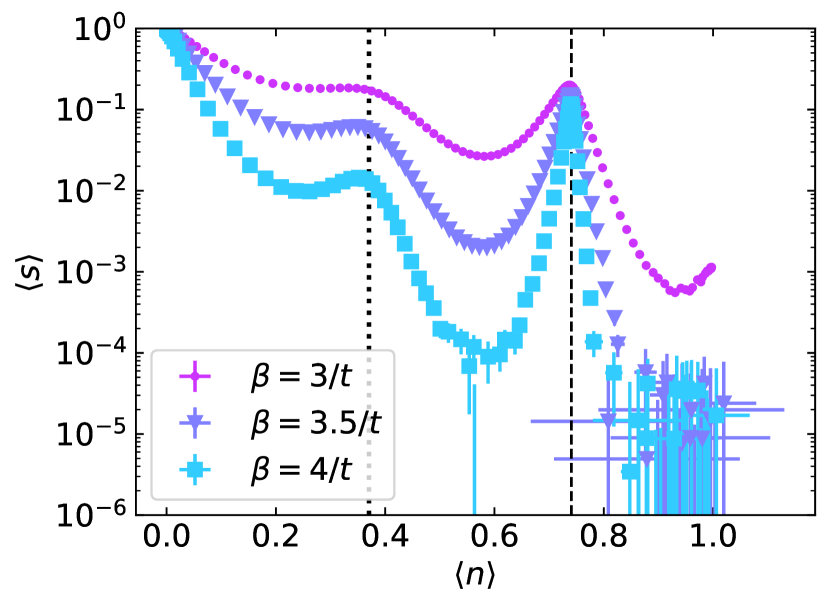
Figure 6: Temperature dependence of fermion sign at field strength $\Phi/\Phi_{0}=30/81$ on $9\times 9$ cluster. Hubbard $U/t=10$. Dotted line marks $\nu=1$ and dashed line marks $\nu=2$.

Historically, there have been limited DQMC studies of the Hubbard model on the triangular lattice (and other non-bipartite lattices), because these systems in general have bad fermion sign problem [79]. The fermion sign worsens with larger cluster size, larger Hubbard $U$, and lower temperatures. In Fig. 6, we show the average fermion sign $\langle s\rangle$ for one set of representative parameters. We observe improvements of fermion sign at more incompressible regions, consistent with previous studies [64, 65]. The sign problem limits the temperatures we can access via DQMC to $\beta\leq 5/t$ at $U=10t$ and $\beta\leq 8/t$ at $U=4t$. As detailed in Appendix B, we run a large number of sweeps and bins to overcome the sign problem, which allows us to see indicators of ground state properties even at relatively high temperatures accessible via DQMC.

Appendix D DQMC finite-size analysis

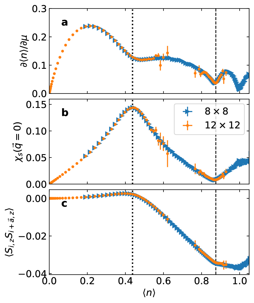
Figure 7: Comparison of DQMC results obtained on $8\times 8$ and $12\times 12$ clusters for a charge compressibility, b uniform spin susceptibility, and c nearest neighbor spin correlation. Fixed field strength $\Phi/\Phi_{0}=28/64=63/144$, Hubbard interaction $U/t=10$ and inverse temperature $\beta=3/t$. Dotted line marks $\nu=1$ and dashed line marks $\nu=2$.

As discussed in [65], the finite-size effect in DQMC simulations of the HH model depends on magnetic field strength $\Phi/\Phi_{0}$ and interaction strength $U/t$. In particular, the finite-size effect is in general smaller for “more incommensurate” values of $\Phi/\Phi_{0}$. This means that it is advantageous, from the perspective of minimizing finite-size effect on a fixed-size cluster, to consider magnetic field strength $\Phi/\Phi_{0}=p/q$ with a large denominator $q$, where $p$ and $q$ are co-prime. Intuitively, we may understand this effect by noting that a large $q$ breaks the crystal Brillouin zone into magnetic Brillouin zones which are $q$ times smaller. This removes artificial degeneracies caused by the limited momentum resolution in a small cluster (termed “shell effect” in [79]). This has been exploited in [67, 80], where one magnetic flux quantum was introduced to reduce finite-size effects for zero-field models. Fig. 7 shows the minimal cluster size dependence of charge compressibility and uniform spin susceptibility at a typical parameter combination. This and many other similar checks allow us to be confident that our conclusions are valid in the thermodynamic limit.

Appendix E Non-interacting results

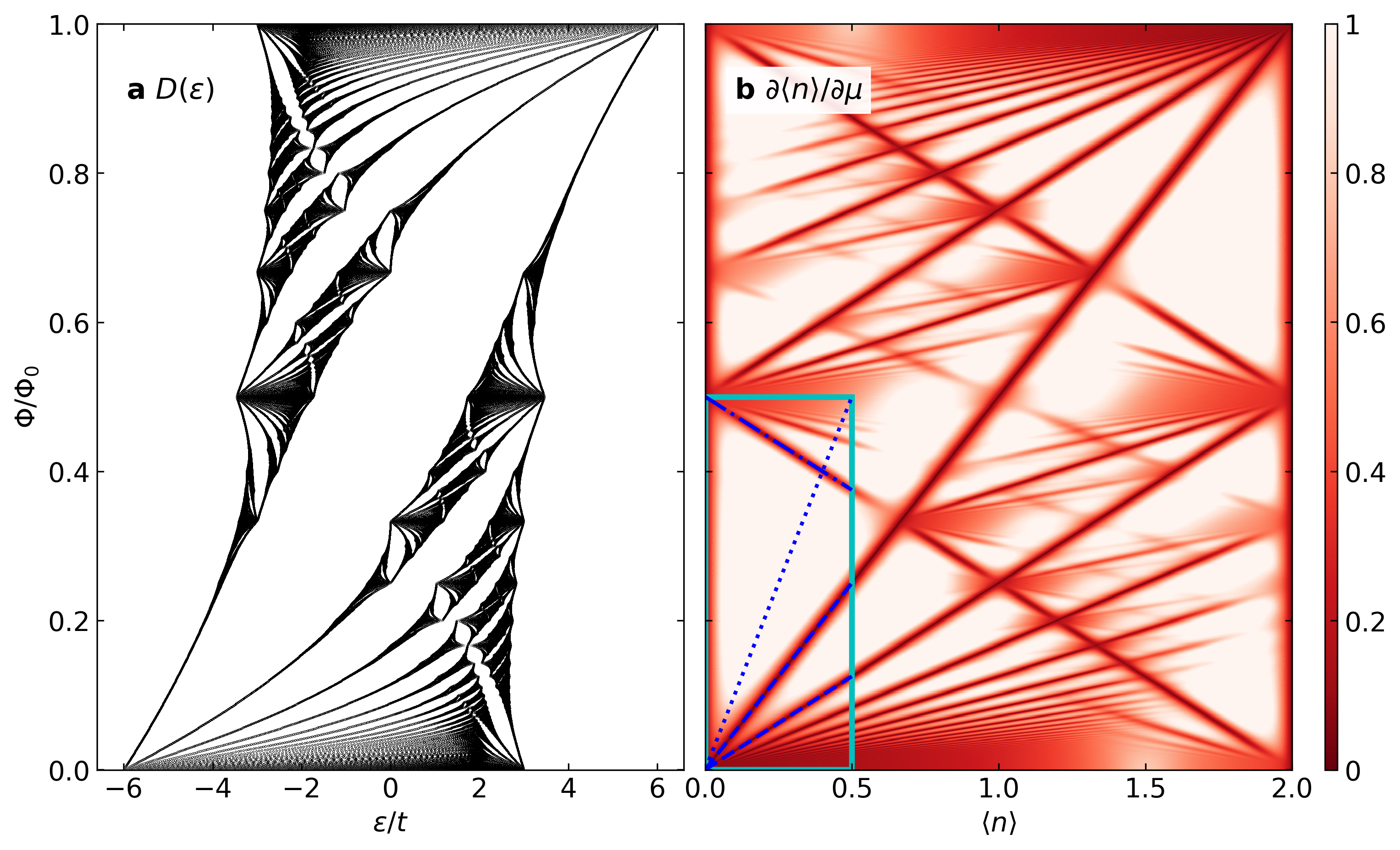
Figure 8: Noninteracting Hofstadter model band structure. a density of states, AKA Hofstadter butterfly, and b Wannier diagram with 2-fold spin degeneracy, at inverse temperature $\beta=20/t$. In b, the cyan box demarcate the region of parameter space we focus on in this study; dotted blue line denotes $\nu=1$, dashed lines denote $\nu=2$ and $\nu=4$, while dot-dashed line denotes $n=-4(\Phi/\Phi_{0})+2$, consistent with styles used in the main text.

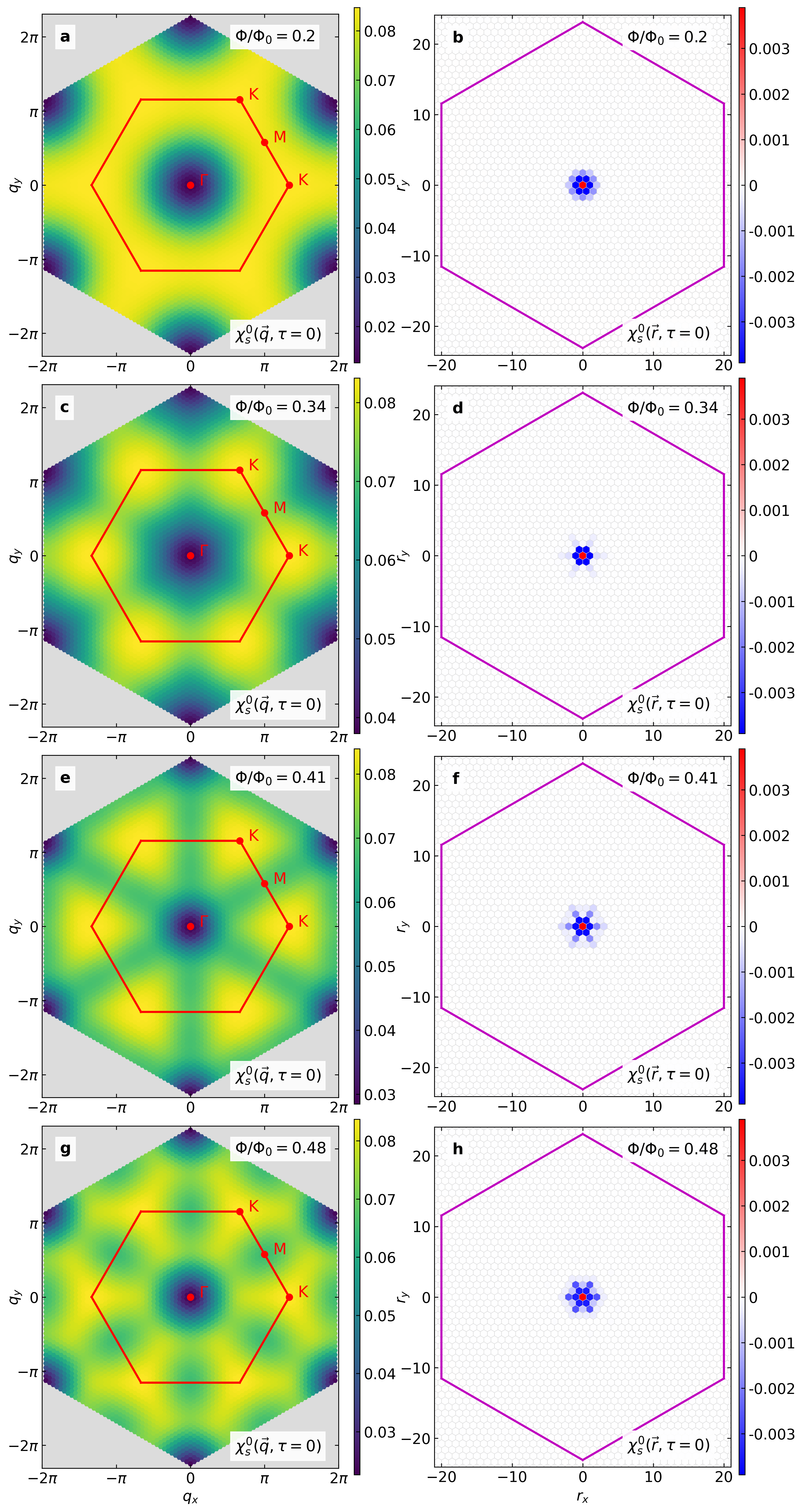
Figure 9: Non-interacting counterpart of Fig. 5 in main text. All plots have fixed inverse temperature $\beta=6/t$, and particle density $\langle n\rangle=0.34$.

In this section, we show the band stucture and Wannier diagram (Fig. 8), and Lindhard susceptibilities (Fig. 9) calculated in the non-interacting Hofstadter model, for easy comparison with results presented in the main text. All results are obtained by diagonalizing the Hofstadter model on a $40\times 40$ cluster.

The non-interacting band structure of the Hofstadter model, as shown in Fig. 8, is $180^{\circ}$ rotation symmetric about $\Phi/\Phi_{0}=0.5$ and $\epsilon=0$ (or $\Phi/\Phi_{0}=0.5$ and $n=1$), reflection symmetric about $\Phi/\Phi_{0}=\pm 1,\pm 3,...$ and periodic along the $\Phi/\Phi_{0}$ direction with a period of 2.

The equal time spin susceptibilities shown in Figs. 5 and 9 are defined as

$$\chi_{s}(\mathbf{r},\tau=0)=\frac{1}{N}\sum_{i}e^{-i\mathbf{q}\cdot\mathbf{r}}\left\langle S_{i,z}S_{i+\mathbf{r},z}\right\rangle,$$ (29)

and

$$\chi_{s}(\mathbf{q},\tau=0) =\frac{1}{N}\sum_{i,j}e^{-i\mathbf{q}\cdot(\mathbf{r}_{i}-\mathbf{r}_{j})}\left\langle S_{i,z}S_{j,z}\right\rangle,$$ (30)

$$=\sum_{\mathbf{r}}e^{-i\mathbf{q}\cdot\mathbf{r}}\chi_{s}(\mathbf{r},\tau=0)$$

where

$$S_{i,z}=\frac{\hbar}{2}\left(c^{\dagger}_{i\uparrow}c_{i\uparrow}-c^{\dagger}_{i\downarrow}c_{i\downarrow}\right).$$ (31)

Appendix F Supplemental data

Charge compressibility $\partial\langle n\rangle/\partial\mu$ is measured in DQMC using the formula

$$\frac{\partial\langle n\rangle}{\partial\mu}=\frac{\beta}{N}\sum_{ij}\left[\langle n_{i}n_{j}\rangle-\langle n_{i}\rangle\langle n_{j}\rangle\right].$$ (32)

Plots of charge compressibility at fixed temperature and for $U/t=4$-$10$ are shown as Wannier diagrams (Fig. 10) and “correlated Hofstadter butterflies” (Fig. 11). The temperature dependence of charge compressibility at fixed magnetic field strength is shown in Fig. 12.

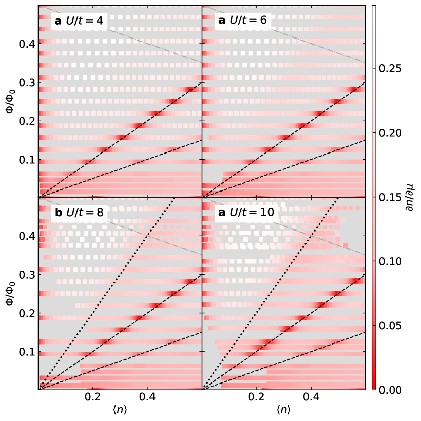
Figure 10: Wannier diagram for Hubbard $U/t=4$ to $U/t=10$. Color: charge compressibity $\partial\langle n\rangle/\partial\mu$. Fixed inverse temperature $\beta=4/t$. Dotted lines denote $\nu=1$, dashed lines denote $\nu=2$ and $\nu=4$, and dot-dashed lines denote $n=-4(\Phi/\Phi_{0})+2$. Grey regions are where we don’t have simulation data. All subplots share the same colorbar. DQMC data are obtained on clusters of size $8\times 8$ and $9\times 9$.

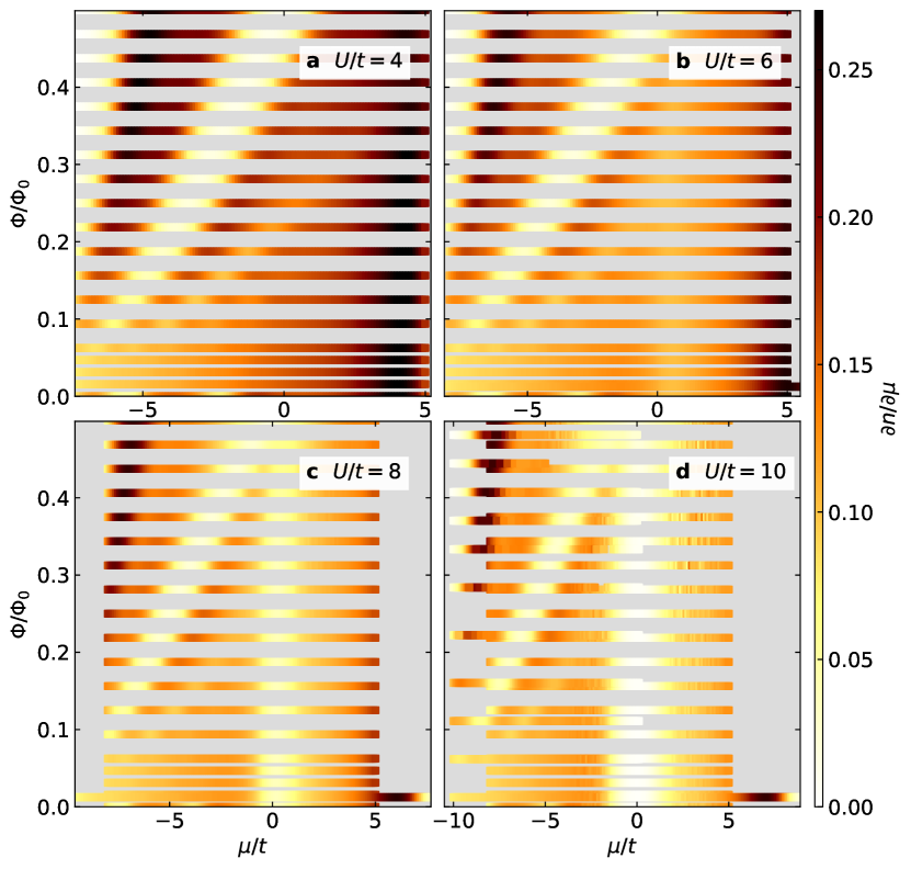
Figure 11: Correlated Hofstadter butterfly for Hubbard $U/t=4$ to $U/t=10$. Color: charge compressibity $\partial\langle n\rangle/\partial\mu$. Fixed inverse temperature $\beta=3/t$. Grey regions are where we don’t have simulation data. All subplots share the same colorbar. DQMC data are obtained on clusters of size $8\times 8$ and $9\times 9$.

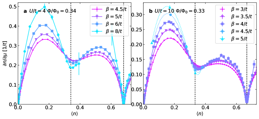
Figure 12: Temperature dependence of charge compressibility $\partial n/\partial\mu$ at fixed magnetic field strength $\Phi/\Phi_{0}\approx 0.33$ for a $U/t=4$ and b $U/t=10$. Dotted black lines denote $\nu=1$, and dashed black lines denote $\nu=2$. DQMC data are obtained on a $12\times 12$ cluster and b $8\times 8$ and $9\times 9$ clusters, respectively. In b, dotted lines going through data points for $\beta=4.5/t$ and $\beta=5/t$ are guides to the eye obtained via cubic spline fitting.

Extended temperature dependence of nearest neighbor spin correlation, obtained via DQMC, is shown in Fig. 13.

Extended Hubbard interaction dependence of nearest neighbor spin correlation, obtained via DQMC, is shown in Fig. 14.

Extended Hubbard interaction dependence of $|q_{\mathrm{max}}|$, obtained via DQMC, is shown in Fig. 15.

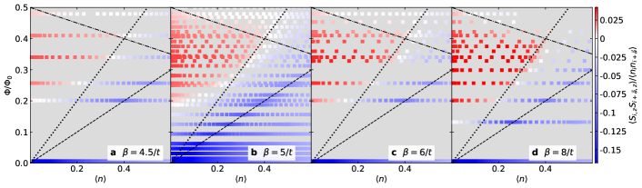
Figure 13: Extended temperature dependence of equal-time nearest-neighbor spin correlation normalized by nearest-neighbor charge correlation, $\langle S_{i,z}S_{i+\mathbf{a},z}\rangle/\langle n_{i}n_{i+\mathbf{a}}\rangle$, obtained by DQMC. Fixed Hubbard $U/t=4$. Dotted lines denote $\nu=1$, dashed lines denote $\nu=2$, and dot-dashed lines denote $n=-4(\Phi/\Phi_{0})+2$. The colorbar is saturated in the minimum direction. DQMC data are obtained on clusters of size $8\times 8$ and $12\times 12$.

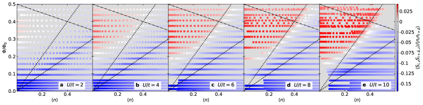
Figure 14: Extended Hubbard $U$ dependence of equal-time nearest-neighbor spin correlation normalized by nearest-neighbor charge correlation, $\langle S_{i,z}S_{i+\mathbf{a},z}\rangle/\langle n_{i}n_{i+\mathbf{a}}\rangle$, obtained by DQMC. Fixed inverse temperature $\beta=4/t$. Dotted lines denote $\nu=1$, dashed lines denote $\nu=2$, and dot-dashed lines denote $n=-4(\Phi/\Phi_{0})+2$. The colorbar is saturated in the minimum direction. DQMC data are obtained on clusters of size $6\times 6$, $8\times 8$, and $9\times 9$.

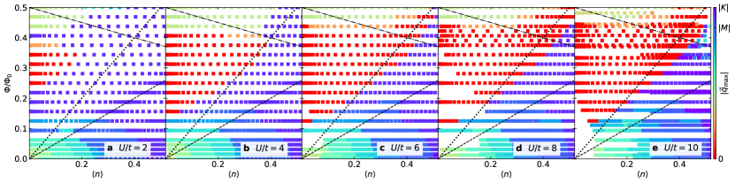
Figure 15: Extended Hubbard $U$ dependence of $|q_{\mathrm{max}}|$, obtained by DQMC. Fixed inverse temperature $\beta=4/t$. Dotted lines denote $\nu=1$, dashed lines denote $\nu=2$, and dot-dashed lines denote $n=-4(\Phi/\Phi_{0})+2$. DQMC data are obtained on clusters of size $8\times 8$ and $9\times 9$.

References

- Tong [2016] D. Tong, Lectures on the quantum hall effect (2016), arXiv:1606.06687 [hep-th] .
- Girvin et al. [1986] S. M. Girvin, A. H. MacDonald, and P. M. Platzman, Magneto-roton theory of collective excitations in the fractional quantum Hall effect, Physical Review B 33, 2481 (1986).
- Parameswaran et al. [2012] S. A. Parameswaran, R. Roy, and S. L. Sondhi, Fractional Chern insulators and the algebra, Physical Review B 85, 241308(R) (2012).
- Roy [2014] R. Roy, Band geometry of fractional topological insulators, Phys. Rev. B 90, 165139 (2014).
- Claassen et al. [2015] M. Claassen, C. H. Lee, R. Thomale, X.-L. Qi, and T. P. Devereaux, Position-momentum duality and fractional quantum Hall effect in Chern insulators, Phys. Rev. Lett. 114, 236802 (2015).
- Wang et al. [2021] J. Wang, J. Cano, A. J. Millis, Z. Liu, and B. Yang, Exact Landau level description of geometry and interaction in a flatband, Physical Review Letters 127, 246403 (2021).
- Ledwith et al. [2022] P. J. Ledwith, A. Vishwanath, and D. E. Parker, Vortexability: A unifying criterion for ideal fractional Chern insulators (2022), arxiv:2209.15023 .
- Hofstadter [1976] D. R. Hofstadter, Energy levels and wave functions of Bloch electrons in rational and irrational magnetic fields, Physical Review B 14, 2239 (1976).
- Wannier [1978] G. H. Wannier, A result not dependent on rationality for Bloch electrons in a magnetic field, Physica Status Solidi (b) 88, 757 (1978).
- Zak [1964] J. Zak, Magnetic translation group, Physical Review 134, A1602 (1964).
- Xiao et al. [2010] D. Xiao, M.-C. Chang, and Q. Niu, Berry phase effects on electronic properties, Rev. Mod. Phys. 82, 1959 (2010).
- Kapit and Mueller [2010] E. Kapit and E. Mueller, Exact parent hamiltonian for the quantum Hall states in a lattice, Physical Review Letters 105, 215303 (2010).
- Bauer et al. [2016] D. Bauer, T. S. Jackson, and R. Roy, Quantum geometry and stability of the fractional quantum Hall effect in the Hofstadter model, Physical Review B 93, 235133 (2016).
- Regnault and Bernevig [2011] N. Regnault and B. A. Bernevig, Fractional Chern insulator, Physical Review X 1, 021014 (2011).
- Sheng et al. [2011] D. N. Sheng, Z.-C. Gu, K. Sun, and L. Sheng, Fractional quantum Hall effect in the absence of Landau levels, Nature Communications 2, 389 (2011).
- Qi [2011] X.-L. Qi, Generic wave-function description of fractional quantum anomalous Hall states and fractional topological insulators, Physical Review Letters 107, 126803 (2011).
- Scaffidi and Möller [2012] T. Scaffidi and G. Möller, Adiabatic continuation of fractional Chern insulators to fractional quantum Hall states, Phys. Rev. Lett. 109, 246805 (2012).
- Möller and Cooper [2015] G. Möller and N. R. Cooper, Fractional Chern insulators in Harper-Hofstadter bands with higher Chern number, Physical Review Letters 115, 126401 (2015).
- Andrews and Möller [2018] B. Andrews and G. Möller, Stability of fractional Chern insulators in the effective continuum limit of Harper-Hofstadter bands with Chern number , Physical Review B 97, 035159 (2018).
- Andrews et al. [2021] B. Andrews, T. Neupert, and G. Möller, Stability, phase transitions, and numerical breakdown of fractional Chern insulators in higher Chern bands of the Hofstadter model, Physical Review B 104, 125107 (2021).
- Bauer et al. [2022] D. Bauer, S. Talkington, F. Harper, B. Andrews, and R. Roy, Fractional Chern insulators with a non-Landau level continuum limit, Physical Review B 105, 045144 (2022).
- Sondhi et al. [1993] S. L. Sondhi, A. Karlhede, S. A. Kivelson, and E. H. Rezayi, Skyrmions and the crossover from the integer to fractional quantum Hall effect at small Zeeman energies, Phys. Rev. B 47, 16419 (1993).
- Nuckolls et al. [2020] K. P. Nuckolls, M. Oh, D. Wong, B. Lian, K. Watanabe, T. Taniguchi, B. A. Bernevig, and A. Yazdani, Strongly correlated Chern insulators in magic-angle twisted bilayer graphene, Nature 588, 610 (2020).
- Choi et al. [2021] Y. Choi, H. Kim, Y. Peng, A. Thomson, C. Lewandowski, R. Polski, Y. Zhang, H. S. Arora, K. Watanabe, T. Taniguchi, J. Alicea, and S. Nadj-Perge, Correlation-driven topological phases in magic-angle twisted bilayer graphene, Nature 589, 536 (2021).
- Park et al. [2021] J. M. Park, Y. Cao, K. Watanabe, T. Taniguchi, and P. Jarillo-Herrero, Flavour Hund’s coupling, Chern gaps and charge diffusivity in moiré graphene, Nature 592, 43 (2021).
- Das et al. [2021] I. Das, X. Lu, J. Herzog-Arbeitman, Z.-D. Song, K. Watanabe, T. Taniguchi, B. A. Bernevig, and D. K. Efetov, Symmetry-broken Chern insulators and Rashba-like Landau-level crossings in magic-angle bilayer graphene, Nature Physics 17, 710 (2021).
- Wu et al. [2021] S. Wu, Z. Zhang, K. Watanabe, T. Taniguchi, and E. Y. Andrei, Chern insulators, van Hove singularities and topological flat bands in magic-angle twisted bilayer graphene, Nature Materials 20, 488 (2021).
- Saito et al. [2021] Y. Saito, J. Ge, L. Rademaker, K. Watanabe, T. Taniguchi, D. A. Abanin, and A. F. Young, Hofstadter subband ferromagnetism and symmetry-broken Chern insulators in twisted bilayer graphene, Nature Physics 17, 478 (2021).
- Stepanov et al. [2021] P. Stepanov, M. Xie, T. Taniguchi, K. Watanabe, X. Lu, A. H. MacDonald, B. A. Bernevig, and D. K. Efetov, Competing zero-field Chern insulators in superconducting twisted bilayer graphene, Physical Review Letters 127, 197701 (2021).
- Yu et al. [2022a] J. Yu, B. A. Foutty, Z. Han, M. E. Barber, Y. Schattner, K. Watanabe, T. Taniguchi, P. Phillips, Z.-X. Shen, S. A. Kivelson, and B. E. Feldman, Correlated Hofstadter spectrum and flavour phase diagram in magic-angle twisted bilayer graphene, Nature Physics 18, 825 (2022a).
- Yu et al. [2022b] J. Yu, B. A. Foutty, Y. H. Kwan, M. E. Barber, K. Watanabe, T. Taniguchi, Z.-X. Shen, S. A. Parameswaran, and B. E. Feldman, Spin skyrmion gaps as signatures of intervalley-coherent insulators in magic-angle twisted bilayer graphene (2022b), arXiv:2206.11304 .
- Chatterjee et al. [2020] S. Chatterjee, N. Bultinck, and M. P. Zaletel, Symmetry breaking and skyrmionic transport in twisted bilayer graphene, Physical Review B 101, 165141 (2020).
- Khalaf et al. [2021] E. Khalaf, S. Chatterjee, N. Bultinck, M. P. Zaletel, and A. Vishwanath, Charged skyrmions and topological origin of superconductivity in magic-angle graphene, Science Advances 7, eabf5299 (2021).
- Kwan et al. [2022] Y. H. Kwan, G. Wagner, N. Bultinck, S. H. Simon, and S. A. Parameswaran, Skyrmions in twisted bilayer graphene: Stability, pairing, and crystallization, Physical Review X 12, 031020 (2022).
- Chatterjee et al. [2022] S. Chatterjee, M. Ippoliti, and M. P. Zaletel, Skyrmion superconductivity: DMRG evidence for a topological route to superconductivity, Physical Review B 106, 035421 (2022).
- Fertig et al. [1997] H. A. Fertig, L. Brey, R. Côté, A. H. MacDonald, A. Karlhede, and S. L. Sondhi, Hartree-Fock theory of skyrmions in quantum Hall ferromagnets, Physical Review B 55, 10671 (1997).
- Abolfath et al. [1997] M. Abolfath, J. J. Palacios, H. A. Fertig, S. M. Girvin, and A. H. MacDonald, Critical comparison of classical field theory and microscopic wave functions for skyrmions in quantum Hall ferromagnets, Phys. Rev. B 56, 6795 (1997).
- Rezayi [1991] E. H. Rezayi, Wave functions and other properties of spin-reversed quasiparticles at Landau-level occupation, Physical Review B 43, 5944 (1991).
- Barrett et al. [1995] S. E. Barrett, G. Dabbagh, L. N. Pfeiffer, K. W. West, and R. Tycko, Optically pumped NMR evidence for finite-size skyrmions in GaAs quantum wells near landau level filling , Phys. Rev. Lett. 74, 5112 (1995).
- Aifer et al. [1996] E. H. Aifer, B. B. Goldberg, and D. A. Broido, Evidence of skyrmion excitations about in -modulation-doped single quantum wells by interband optical transmission, Phys. Rev. Lett. 76, 680 (1996).
- Schmeller et al. [1995] A. Schmeller, J. P. Eisenstein, L. N. Pfeiffer, and K. W. West, Evidence for skyrmions and single spin flips in the integer quantized Hall effect, Phys. Rev. Lett. 75, 4290 (1995).
- Wu and Sondhi [1995] X.-G. Wu and S. L. Sondhi, Skyrmions in higher Landau levels, Physical Review B 51, 14725 (1995).
- Rhone et al. [2015] T. D. Rhone, L. Tiemann, and K. Muraki, NMR probing of spin and charge order near odd-integer filling in the second Landau level, Phys. Rev. B 92, 041301(R) (2015).
- Melik-Alaverdian et al. [1999] V. Melik-Alaverdian, N. E. Bonesteel, and G. Ortiz, Skyrmion physics beyond the lowest Landau-level approximation, Physical Review B 60, R8501 (1999).
- Mihalek and Fertig [2000] I. Mihalek and H. A. Fertig, Landau-level mixing and skyrmion stability in quantum Hall ferromagnets, Physical Review B 62, 13573 (2000).
- Wu and Das Sarma [2020] F. Wu and S. Das Sarma, Quantum geometry and stability of moiré flatband ferromagnetism, Phys. Rev. B 102, 165118 (2020).
- Khalaf and Vishwanath [2022] E. Khalaf and A. Vishwanath, Baby skyrmions in Chern ferromagnets and topological mechanism for spin-polaron formation in twisted bilayer graphene, Nature Communications 13, 6245 (2022).
- Schindler et al. [2022] F. Schindler, O. Vafek, and B. A. Bernevig, Trions in twisted bilayer graphene, Physical Review B 105, 155135 (2022).
- White et al. [1989] S. R. White, D. J. Scalapino, R. L. Sugar, E. Y. Loh, J. E. Gubernatis, and R. T. Scalettar, Numerical study of the two-dimensional Hubbard model, Physical Review B 40, 506 (1989).
- Loh et al. [1990] E. Y. Loh, J. E. Gubernatis, R. T. Scalettar, S. R. White, D. J. Scalapino, and R. L. Sugar, Sign problem in the numerical simulation of many-electron systems, Physical Review B 41, 9301 (1990).
- White [1992] S. R. White, Density matrix formulation for quantum renormalization groups, Phys. Rev. Lett. 69, 2863 (1992).
- White [1993] S. R. White, Density-matrix algorithms for quantum renormalization groups, Phys. Rev. B 48, 10345 (1993).
- Östlund and Rommer [1995] S. Östlund and S. Rommer, Thermodynamic limit of density matrix renormalization, Phys. Rev. Lett. 75, 3537 (1995).
- Dukelsky et al. [1998] J. Dukelsky, M. A. Martín-Delgado, T. Nishino, and G. Sierra, Equivalence of the variational matrix product method and the density matrix renormalization group applied to spin chains, Europhys. Lett. 43, 457 (1998).
- Shaffer et al. [2021] D. Shaffer, J. Wang, and L. H. Santos, Theory of Hofstadter superconductors, Physical Review B 104, 184501 (2021).
- Shaffer et al. [2022] D. Shaffer, J. Wang, and L. H. Santos, Unconventional self-similar Hofstadter superconductivity from repulsive interactions, Nature Communications 13, 7785 (2022).
- Cocks et al. [2012] D. Cocks, P. P. Orth, S. Rachel, M. Buchhold, K. Le Hur, and W. Hofstetter, Time-reversal-invariant Hofstadter-Hubbard model with ultracold fermions, Physical Review Letters 109, 205303 (2012).
- Sahay et al. [2023] R. Sahay, S. Divic, D. E. Parker, T. Soejima, S. Anand, J. Hauschild, M. Aidelsburger, A. Vishwanath, S. Chatterjee, N. Y. Yao, and M. P. Zaletel, Superconductivity in a topological lattice model with strong repulsion (2023), arxiv:2308.10935 .
- Yang et al. [2021] J. Yang, L. Liu, J. Mongkolkiattichai, and P. Schauss, Site-resolved imaging of ultracold fermions in a triangular-lattice quantum gas microscope, PRX Quantum 2, 020344 (2021).
- Garwood et al. [2022] D. Garwood, J. Mongkolkiattichai, L. Liu, J. Yang, and P. Schauss, Site-resolved observables in the doped spin-imbalanced triangular Hubbard model, Phys. Rev. A 106, 013310 (2022).
- Mongkolkiattichai et al. [2022] J. Mongkolkiattichai, L. Liu, D. Garwood, J. Yang, and P. Schauss, Quantum gas microscopy of a geometrically frustrated Hubbard system (2022), arxiv:2210.14895 .
- Xu et al. [2023] M. Xu, L. H. Kendrick, A. Kale, Y. Gang, G. Ji, R. T. Scalettar, M. Lebrat, and M. Greiner, Frustration- and doping-induced magnetism in a Fermi-Hubbard simulator, Nature 620, 971 (2023).
- Mancini et al. [2015] M. Mancini, G. Pagano, G. Cappellini, L. Livi, M. Rider, J. Catani, C. Sias, P. Zoller, M. Inguscio, M. Dalmonte, and L. Fallani, Observation of chiral edge states with neutral fermions in synthetic Hall ribbons, Science 349, 1510 (2015).
- Ding et al. [2022] J. K. Ding, W. O. Wang, B. Moritz, Y. Schattner, E. W. Huang, and T. P. Devereaux, Thermodynamics of correlated electrons in a magnetic field, Communications Physics 5, 204 (2022).
- Mai et al. [2023] P. Mai, E. W. Huang, J. Yu, B. E. Feldman, and P. W. Phillips, Interaction-driven spontaneous ferromagnetic insulating states with odd Chern numbers, npj Quantum Materials 8, 1 (2023).
- Palm et al. [2023] F. A. Palm, M. Kurttutan, A. Bohrdt, U. Schollwöck, and F. Grusdt, Ferromagnetism and skyrmions in the Hofstadter-Fermi-Hubbard model, New Journal of Physics 25, 023021 (2023).
- Assaad [2002] F. F. Assaad, Depleted Kondo lattices: Quantum Monte Carlo and mean-field calculations, Phys. Rev. B 65, 115104 (2002).
- Parameswaran et al. [2013] S. A. Parameswaran, R. Roy, and S. L. Sondhi, Fractional quantum Hall physics in topological flat bands, Comptes Rendus Physique Topological Insulators / Isolants Topologiques, 14, 816 (2013).
- Fishman et al. [2022a] M. Fishman, S. R. White, and E. M. Stoudenmire, The ITensor software library for tensor network calculations, SciPost Phys. Codebases , 4 (2022a).
- Fishman et al. [2022b] M. Fishman, S. R. White, and E. M. Stoudenmire, Codebase release 0.3 for ITensor, SciPost Phys. Codebases , 4 (2022b).
- MacDonald et al. [1996] A. H. MacDonald, H. A. Fertig, and L. Brey, Skyrmions without sigma models in quantum Hall ferromagnets, Phys. Rev. Lett. 76, 2153 (1996).
- Wójs and Quinn [2002] A. Wójs and J. J. Quinn, Spin excitation spectra of integral and fractional quantum Hall systems, Physical Review B 66, 045323 (2002).
- Zhang et al. [2019] Y.-H. Zhang, D. Mao, Y. Cao, P. Jarillo-Herrero, and T. Senthil, Nearly flat Chern bands in moiré superlattices, Physical Review B 99, 075127 (2019).
- Repellin and Senthil [2020] C. Repellin and T. Senthil, Chern bands of twisted bilayer graphene: Fractional Chern insulators and spin phase transition, Phys. Rev. Res. 2, 023238 (2020).
- Okubo et al. [2012] T. Okubo, S. Chung, and H. Kawamura, Multiple- states and the skyrmion lattice of the triangular-lattice Heisenberg antiferromagnet under magnetic fields, Phys. Rev. Lett. 108, 017206 (2012).
- Barkeshli and McGreevy [2012] M. Barkeshli and J. McGreevy, Continuous transitions between composite Fermi liquid and Landau Fermi liquid: A route to fractionalized Mott insulators, Physical Review B 86, 075136 (2012).
- Dong and Levitov [2022] Z. Dong and L. Levitov, Chiral Stoner magnetism in Dirac bands (2022), arxiv:2208.02051 [cond-mat] .
- Zhu et al. [2022] Z. Zhu, D. N. Sheng, and A. Vishwanath, Doped Mott insulators in the triangular-lattice Hubbard model, Physical Review B 105, 205110 (2022).
- Iglovikov et al. [2015] V. I. Iglovikov, E. Khatami, and R. T. Scalettar, Geometry dependence of the sign problem in quantum Monte Carlo simulations, Phys. Rev. B 92, 045110 (2015).
- Schattner et al. [2016] Y. Schattner, M. H. Gerlach, S. Trebst, and E. Berg, Competing orders in a nearly antiferromagnetic metal, Phys. Rev. Lett. 117, 097002 (2016).