Scattered wavefield in the stochastic homogenization regime

Abstract

In the context of providing a mathematical framework for the propagation of ultrasound waves in a random multiscale medium, we consider the scattering of classical waves (modeled by a divergence form scalar Helmholtz equation) by a bounded object with a random composite micro-structure embedded in an unbounded homogeneous background medium. Using quantitative stochastic homogenization techniques, we provide asymptotic expansions of the scattered field in the background medium with respect to a scaling parameter describing the spatial random oscillations of the micro-structure. Introducing a boundary layer corrector to compensate the breakdown of stationarity assumptions at the boundary of the scattering medium, we prove quantitative $L^{2}$- and $H^{1}$- error estimates for the asymptotic first-order expansion. The theoretical results are supported by numerical experiments.

1 Introduction and context

The emergence of quantitative medical imaging techniques that can map the numerical value of a physical parameter in a biological tissue constitutes a major shift of paradigm for the theory of inverse problems. Imaging modalities are now expected not only to produce images that are anatomically accurate (structural images) but also stably and quantitatively reconstruct parameters of interest that can help discriminate pathological states.

Medical ultrasound imaging is a powerful, safe, portable and cheap imaging modality that is used in countless physical exams. Ultrasonic pulses (in the MHz range) are transmitted into the region of interest and the images are obtained by numerically backpropagating the echoes generated by the tissues and recorded on a receiver array. Each tissue and its pathological state will be characterized by a distinct type of speckle on the image.

The technique relies on the fact that most soft tissues have a mass density and compressibility close to those of water (and ultrasonic waves travel in these tissues almost as in water) yet have echogenic properties that can be explained by the presence of acoustic heterogeneities of characteristic size much smaller than the wavelength, see [1].

The quantification of these echogenic properties (known in the literature as backscattering coefficient estimation [2]) relied until now on the introduction of an ultrasonic reflectivity [3] and approximations of the scattered field derived under a set of restrictive hypotheses that do not hold in many practical situations (usually assumptions of the low scatterer concentration, single scattering regime, strictly homogeneous mass density in the medium, uniformity of the excitation beam …[4]). Recently, using a formal approach based on a separation of scale in the scattering process, Aubry $\&$ al. have recently obtained spectacular results in quantitative speed of sound imaging on experimental data [5].

In this paper, we aim at providing a mathematical framework for the propagation of ultrasound waves in random multiscale media. Using the tools of stochastic homogenization, we provide a mathematical model for the acoustic properties of a soft tissue as well as quantitative asymptotic expansions of the scattered field with respect to the scale of the acoustic heterogeneities in the medium.

1.1 State of the art

Homogenization techniques are an essential tool to address the study of partial differential equations with rapidly oscillating coefficients that exhibit periodic [6] or stochastic [7, 8] variations, allowing to derive effective coefficients or asymptotic expansions for the solutions.

In the case of stochastic homogenization, the recent quantification of convergence rates in the case of the Poisson equation in unbounded domains, obtained independently by Armstrong et al [9] as well as Gloria and Otto [10, 11] has initiated a leap in results on the subject, relaxing some of the hypotheses of the aforementioned papers. Using multiscale inequalities to quantify ergodicity, quantitative convergence rates were obtained for correlated coefficients with long range correlations [12, 13] or in the case of bounded domains [14, 15]. Additionally, the emergence of a theory of fluctuations in stochastic homogenization has lead to introducing a new quantity : the homogenization commutator. In the series of articles [16, 17] the authors have shown that the fluctuations of the two-scale expansion error of the so-called commutator characterizes the fluctuations of all the observables of interest (flux, gradient…).

Classical wave scattering by a medium containing periodically distributed penetrable objects has attracted a lot of attention in the recent years [18, 19, 20] with a particular focus on the asymptotic analysis of the boundary corrector [21] and the construction of effective transmission conditions [22]. We also refer to [23, 24, 25] for major contributions to the study of the boundary layers for the Poisson equation.

1.2 Main contribution

In this paper, we are interested in the scattering of classical waves by a bounded object with a random composite micro-structure embedded in an unbounded homogeneous background medium. The problem considered is modeled by a divergence form scalar Helmholtz equation with discontinuous rapidly oscillating (at some scale $\varepsilon$ much smaller than the wavelength) stochastic coefficients.

Building on the methods developed in [26, 12] we establish a first-order (with respect to the parameter $\varepsilon$) asymptotic expansion of the scattered field inside the object (proposition 2). Introducing a boundary layer corrector to enforce transmission conditions at the boundary of the object we prove $L^{2}$- and $H^{1}$-norm convergence rates (proposition 6). Using the Lippman-Schwinger equation and results on fluctuations of the commutator [16], we derive a quantitative first-order expansion of the scattered wave outside the object. We also present numerical illustrations of the solution of the multiscale problem as well as the correctors, and the first-order expansion of the solution. Numerical convergence rates are computed to support the theoretical claims.

The article is organized as follows:

• In section 2 we present the model for the propagation medium and the stochastic framework required to prove stochastic homogenization results.

• Section 3 is devoted to proving $L^{2}$- and $H^{1}$- quantitative estimates of the error between the solution of the original problem and the first-order two-scale expansion (proposition 7).

• Using the expansions of the solution and its gradient inside the composite medium established in the previous section in conjonction with the Lippman-Schwinger equation satisfied by the scattered field eq (78), we derive in section 4 an explicit integral representation formula for an $H^{1}$- approximation of the scattered field outside the composite medium of order $(d+1)/2$ (Theorem 10), where $d$ is the dimension. This theorem along with Corollary 11 is the main result of the paper. It makes it possible to relate the small-scale fluctuations of the composite medium and the scattered wavefield that can be measured outside the medium. This paves the way towards the resolution of quantitative inverse problems that aim at characterizing the statistics of the composite medium from the statistics of the scattered field.

• In section 5, we show numerical results on the original problem, the effective coefficients and the homogenized problem, as well as the different correctors. We compute the different norm errors between the solution of the original problem and its various approximations to confirm the claims of proposition 8 and theorem 10.

Contents

1. 1 Introduction and context
   1. 1.1 State of the art
   2. 1.2 Main contribution
2. 2 Presentation of the model
   1. 2.1 Description of the distribution of scatterers
   2. 2.2 Stochastic setting
3. 3 Two-scale asymptotic expansion of the field
   1. 3.1 Homogenized problem
   2. 3.2 Two-scale expansion error and boundary layer
   3. 3.3 Two-scale error - boundary corrector
   4. 3.4 Convergence rate of the two-scale expansion
4. 4 Asymptotic expansion of the scattered field
   1. 4.1 Main result
   2. 4.2 Representation formula for $\delta\mathcal{P}$
   3. 4.3 Proof of Theorem 10
5. 5 Numerical illustrations
   1. 5.1 Geometry and choice of parameters
   2. 5.2 Computation of the reference solution
   3. 5.3 Computation of the correctors and effective parameters
   4. 5.4 Numerical results
6. A Well-posedness of the scattering problem and $H^{s}$-regularity
7. B Qualitative homogenization
8. C Homogenization with a less regular solution
9. D Proof of Lemma 12

2 Presentation of the model

We consider a bounded acoustic medium $D\subset\mathbb{R}^{d}$, $d\in[\![1,3]\!]$ with a $\mathcal{C}^{4}$- boundary $\partial D$ and we study the scattering of a time-harmonic plane wave

$$u^{inc}(x):=exp(ik\theta\cdot x)~{}\textrm{ for }x\in\mathbb{R}^{d}$$ (1)

with wave number $k$ and direction $\theta\in\mathbb{S}$. We assume that a set $S^{\varepsilon}$ of randomly distributed inclusions of characteristic size $\varepsilon>0$ lies inside the medium $D$. $\varepsilon$ is small compared to the wavelength of the incoming field $2\pi k^{-1}$.

Figure 1: Scattering by an obstacle in the stochastic homogenization regime

The outer medium $\mathbb{R}^{d}\setminus\overline{D}$, the background $D\setminus\overline{S^{\varepsilon}}$ and the scatterers $S^{\varepsilon}$ are assumed to be homogeneous with respective parameters $(Id,n_{0})$, $(a_{M},n_{M})$ and $(a_{S},n_{S})$. The medium parameters are then given by

$$\left\{\begin{array}[]{l}\displaystyle\vspace{0.2cm}a_{\varepsilon}:=Id\mathbbm{1}_{\mathbb{R}^{d}\setminus\overline{D}}+a_{M}\mathbbm{1}_{D\setminus\bar{S^{\varepsilon}}}+a_{S}\mathbbm{1}_{S^{\varepsilon}},\\ \displaystyle\vspace{0.2cm}n_{\varepsilon}:=n_{0}\mathbbm{1}_{\mathbb{R}^{d}\setminus\overline{D}}+n_{M}\mathbbm{1}_{D\setminus\bar{S^{\varepsilon}}}+n_{S}\mathbbm{1}_{S^{\varepsilon}},\end{array}\right.$$ (2)

where $a_{M}$ and $a_{S}$ are positive definite matrices of $\mathcal{M}_{d}(\mathbb{R})$ and $n_{0}$, $n_{M}$, $n_{S}$ are positive.
The total field $u_{\varepsilon}$ is then the unique solution a.s. in $H^{1}_{loc}(\mathbb{R}^{d})$ of the following problem:

$$\left\{\begin{aligned} &-\nabla\cdot\left(a_{\varepsilon}(x)\nabla u_{\varepsilon}(x)\right)-k^{2}n_{\varepsilon}(x)u_{\varepsilon}(x)=0&&\textrm{for }x\in\mathbb{R}^{d},\\ &\lim_{|x|\to+\infty}|x|^{\frac{d-1}{2}}\left(\frac{\partial(u_{\varepsilon}-u^{inc})}{\partial|x|}(x)-ik~{}(u_{\varepsilon}-u^{inc})(x)\right)=0.\end{aligned}\right.$$ (3)

Remark 1.

In the context of acoustics $u_{\varepsilon}$ is the pressure. $a_{\varepsilon}$ and $n_{\varepsilon}$ relate to the mass density and the bulk modulus of the inner and outer media [27, Chapter 3.3]. We choose identical parameters for all scatterers. The study can easily be extended to independent and identically distributed parameters as long as the assumptions of uniform ellipticity for $a_{\varepsilon}$ and uniform boundness from below and above for $n_{\varepsilon}$ are satisfied.

We will derive an asymptotic expansion of $u_{\varepsilon}(x)$ with respect to $\varepsilon$ for $x\in\mathbb{R}^{d}\setminus\overline{D}$ using quantitative stochastic homogenization techniques. Before doing so, let us specify in this section the different assumptions that we make on the random distribution of scatterers.

2.1 Description of the distribution of scatterers

Let $(x_{i})_{i\in\mathbb{N}}$ be the point process in $\mathbb{R}^{d}$ corresponding to the centers of the scatterers. A scatterer $s_{i}$, $i\in\mathbb{N}$ centered at $x_{i}$ consists in an open connected Lipschitz domain $\mathcal{O}$ of radius $r:=\underset{x,y\in\mathcal{O}}{\max}|x-y|$. We denote by $S:=\underset{i\in\mathbb{N}}{\cup}s_{i}$ the set of scatterers of radius $r=1$ in $\mathbb{R}^{d}$. Let $(\Omega,\mathcal{F},\mathbb{P})$ be a probability space. We make the following assumptions on $(x_{i})_{i\in\mathbb{N}}$:

• $(x_{i})_{i\in\mathbb{N}}$ is stationary, i.e. its distribution law is invariant by translation and ergodic;

• the scatterers lie at a distance at least $\delta>0$ from one another, i.e. there exists $\delta>0$ such that

  $$\forall i\neq j,~{}dist(s_{i},s_{j})>\delta\quad\textrm{a.s.}$$

We introduce the parameters

$$\left\{\begin{array}[]{l}\displaystyle\vspace{0.2cm}a:=a_{M}\mathbbm{1}_{\mathbb{R}^{d}\setminus\overline{S}}+a_{S}\mathbbm{1}_{S},\\ \displaystyle\vspace{0.2cm}n:=n_{M}\mathbbm{1}_{\mathbb{R}^{d}\setminus\overline{S}}+n_{S}\mathbbm{1}_{S}.\\ \end{array}\right.$$ (4)

For $\varepsilon>0$, we define

$$\mathcal{N}_{\varepsilon}:=\{i\in\mathbb{N}~{}|~{}\varepsilon x_{i}\in D\}.$$

$\mathcal{N}_{\varepsilon}$ corresponds to the collection of scatterers of size $\varepsilon$ that lie in $D$. We subsequently denote

$$S^{\varepsilon}:=\underset{i\in\mathcal{N}_{\varepsilon}}{\cup}\varepsilon s_{i}\cap D.$$ (5)

Note that we have then

$$\forall x\in D,~{}a_{\varepsilon}(x)=a\biggl{(}\frac{x}{\varepsilon}\biggr{)}\textrm{ and }n_{\varepsilon}(x)=n\biggl{(}\frac{x}{\varepsilon}\biggr{)}.$$

Figure 2(b) illustrate an example of a realization of $a_{\varepsilon}$ in $D$.

2.2 Stochastic setting

As it is customary in stochastic homogenization, we define stationarity and ergodicity through an action $(\tau_{x})_{x\in\mathbb{R}^{d}}$ of the group $(\mathbb{R}^{d},+)$ on $(\Omega,\mathcal{F})$.
We thus equip $(\Omega,\mathcal{F})$ with $(\tau_{x})_{x\in\mathbb{R}^{d}}$ that verifies:

• the map $\tau:\displaystyle\left\{\begin{array}[]{ccc}\vspace{0.2cm}\mathbb{R}^{d}\times\Omega&\to&\Omega\\ ({x},\omega)&\mapsto&\tau_{x}\omega\end{array}\right.$ is measurable,

• $\forall x,y\in\mathbb{R}^{d},\tau_{x+y}=\tau_{x}\circ\tau_{y},$

• For all $x\in\mathbb{R}^{d}$, $\tau_{x}$ preserves $\mathbb{P}$, i.e.

  $$\forall A\in\mathcal{F},\,\,\mathbb{P}(\tau_{x}A)=\mathbb{P}(A).$$

Definition 1 (Stationarity).

In the rest of the paper, a random process $f:\mathbb{R}^{d}\times\Omega\to\mathbb{R}^{p}$ is said to be stationary (with respect to $\tau$) if

$$\forall x,y\in\mathbb{R}^{d},\,\text{a.e.}\,\omega\in\Omega,\,\,f(x+y,\omega)=f(x,\tau_{y}\omega).$$ (6)

Moreover, we assume that the action $(\tau_{x})_{x\in\mathbb{R}^{d}}$ is ergodic.

Definition 2 (Ergodicity).

Any $\tau$-invariant event has probability 0 or 1, that is,

$$\forall A\in\mathcal{F},\,\,(\forall x\in\mathbb{R}^{d},\,\,\tau^{-1}_{x}A=A)\implies(\mathbb{P}(A)\in\{0,1\}).$$ (7)

We can now write in terms of $\tau$ the stationary and ergodic assumption on $\left\{x_{i}^{\omega}\right\}_{i\in\mathbb{N}}$ the centers of the scatterers for the realization $\omega\in\Omega$.

$$\forall\omega\in\Omega,~{}\forall y\in\mathbb{R}^{d},~{}\left\{x_{i}^{\omega}+y\right\}_{i\in\mathbb{N}}=\left\{x_{i}^{\tau_{y}\omega}\right\}_{i\in\mathbb{N}}.$$ (8)

These two assumptions are the minimal and classical assumptions on the distribution of scatterers $(x_{i})_{i\in\mathbb{N}}$ that we require for qualitative stochastic homogenization. In the rest of the paper the dependency on randomness $\omega\in\Omega$ is not mentioned explicitly.

We also assume that the process $(x_{i})_{i\in\mathbb{N}}$ or equivalently $S$ verifies a quantitative mixing condition. We choose to express this condition as a multiscale variance inequality as introduced in [28]. This assumption is verified by the most common hardcore point processes such as Matèrn point process [29, Section 6.5.2] as proved in [28, Section 3].

Hypothesis 1 (Mixing hypothesis).

There exists a non-increasing weight function $\pi:\mathbb{R}^{+}\to\mathbb{R}^{+}$ with exponential decay such that $S$ verifies for all $\sigma(S)$- measurable random variable $F(S)$,

$$\textrm{Var}\left[F(S)\right]\leq\mathbb{E}\left[\int_{1}^{+\infty}\int_{\mathbb{R}^{d}}\left(\partial^{osc}_{S,B_{\ell}(x)}F(S)\right)^{2}\mathrm{d}x\ell^{-d}\pi(\ell-1)\mathrm{d}\ell\right],$$ (9)

where $B_{\ell}(x)$ is the ball with radius $\ell\geq 0$ and center $x\in\mathbb{R}^{d}$ and the oscillation $\partial^{osc}_{S,B_{l}(x)}F(S)$ of $F(S)$ with respect to $S$ on $B_{\ell}(x)$ is defined by:

$$\partial^{osc}_{S,B_{l}(x)}F(S):=\textrm{sup ess}\left\{F(S^{\prime})|S^{\prime}\cap(\mathbb{R}^{d}\setminus B_{\ell}(x))=S\cap(\mathbb{R}^{d}\setminus B_{\ell}(x))\right\}\\ -\textrm{inf ess}\left\{F(S^{\prime})|S^{\prime}\cap(\mathbb{R}^{d}\setminus B_{\ell}(x))=S\cap(\mathbb{R}^{d}\setminus B_{\ell}(x))\right\}.$$

Proposition 1 (Matèrn process [28, Proposition 3.3]).

The Matèrn process verifies (9) with the weight function $\pi$:

$$\pi(l)=Ce^{-\frac{1}{C}l}$$ (10)

for some $C>0$.

Remark 2.

Note that the Hypothesis 1 implies that the covariance function of $S$ : $C_{S}(x):=\textrm{Cov}(S(0),S(x))$ satisfies [30, Proposition 1.3]

$$\forall x\in\mathbb{R}^{d},~{}|C_{S}(x)|\lesssim\int_{\max(\frac{1}{2}(|x|-2),0)}^{\infty}\pi(\ell)\mathrm{d}\ell.$$ (11)

where the notation $\lesssim$ stands for "inferior up to a multiplicative constant dependent only on the dimension and possibly other controlled quantities" and will be used throughout the paper. For a Matèrn process this implies that $C_{S}$ has an exponential decay.

3 Two-scale asymptotic expansion of the field

3.1 Homogenized problem

We restrict our domain of study to $B_{R}$ the ball of radius $R>0$ centered at $0$, via the Dirichlet-to-Neumann operator $\Lambda:H^{\frac{1}{2}}(\partial B_{R})\to H^{-\frac{1}{2}}(\partial B_{R})$. This operator takes a Dirichlet data $g\in H^{\frac{1}{2}}(B_{R})$ and maps it to the Neumann trace of $u$ on $\partial B_{R}$ i.e. ${\Lambda g=\nabla u\cdot\nu\in H^{-\frac{1}{2}}(\partial B_{R})}$ where $u$ is the outgoing the solution of

$$-\Delta u-k^{2}n_{0}u=0\textrm{ in }\mathbb{R}^{d}\setminus{\overline{B_{R}}},\textrm{ satisfying }u|_{\partial B_{R}}=g.$$

$\Lambda$ is continuous, self-adjoint and non-positive and its expansion in terms of Hankel functions can be found for example in [31], [32, Section 2.6.3] and [33].
We thus consider $u_{\varepsilon}$ the a.s. unique solution in $H^{1}(B_{R})$ to

$$\left\{\begin{aligned} &-\nabla\cdot\left(a_{\varepsilon}\nabla u_{\varepsilon}\right)-k^{2}n_{\varepsilon}u_{\varepsilon}=0&&\textrm{in }B_{R},\\ &\nabla(u_{\varepsilon}-u^{inc})\cdot\nu=\Lambda(u_{\varepsilon}-u^{inc})&&\textrm{on }\partial B_{R}.\\ \end{aligned}\right.$$ (12)

The well-posedness of (12) for non-smooth coefficients is a difficult problem in $3d$. We refer to [34] for the proof in the $L^{\infty}$ case. However, the proof relies on Fredholm theory and unique continuation principle and therefore does not yield a uniform explicit control with respect to $\varepsilon$ and $\omega$. To obtain this type of uniform control that will be necessary for the homogenization process, we have to add some additional assumptions on the coefficients. For $kR$ sufficiently small or $\Im k>0$ the sesquilinear form associated to (12) can be proved to be coercive and the uniform bound in $\varepsilon$ and $\omega$ of $u_{\varepsilon}$ can be achieved [35]. We also point out that some other methods were developed in [35] and [36] to obtain uniform control of the solution, but they do not apply to our specific problem. Here, we assume that the sesquilinear form associated to (12) is coercive so that Proposition 14 holds. The following homogenization theorem follows directly.

Proposition 2 (Qualitative homogenization theorem).

A.s. the unique solution $u_{\varepsilon}\in H^{1}(B_{R})$ of (12) converges weakly in $H^{1}(B_{R})$ towards $u_{0}$, the unique solution in $H^{1}(B_{R})$ of the following problem

$$\left\{\begin{aligned} &-\Delta u_{0}-k^{2}n_{0}u_{0}=0&&\textrm{in }B_{R}\setminus\overline{D},\\ &-\nabla\cdot\left(a^{hom}\nabla u_{0}\right)-k^{2}n^{hom}u_{0}=0&&\textrm{in }D,\\ &u_{0}^{-}-u_{0}^{+}=0&&\textrm{on }\partial D,\\ &\nabla u_{0}^{-}\cdot\nu-a^{hom}\nabla u_{0}^{+}\cdot\nu=0&&\textrm{on }\partial D,\\ &\nabla(u_{0}-u^{inc})\cdot\nu=\Lambda(u_{0}-u^{inc})&&\textrm{on }\partial B_{R},\\ \end{aligned}\right.$$ (13)

where the superscripts ^- and ⁺ denote the traces outside and inside $D$.
The homogenized coefficients $a^{hom}\in\mathcal{M}_{d}(\mathbb{R})$ and $n^{hom}\in(0,+\infty)$ are defined as follows

$$\left\{\begin{aligned} a^{hom}_{i,j}&=\mathbb{E}[e_{j}\cdot a(e_{i}+\nabla\phi_{i})],\\ n^{hom}&=\mathbb{E}[n],\end{aligned}\right.$$ (14)

and for $i\in[\![1,d]\!]$ the corrector $\phi_{i}$ is defined as in the forthcoming Definition 3.

We define for any integrable function $f$ and any domain $B$ the notation $\fint_{B}f$ as

$$\fint_{B}f:=\frac{1}{|B|}\int_{B}f.$$

Definition 3 (Corrector).

Let $(\phi_{i})_{i\in[\![1,d]\!]}$ be the unique vector field such that for all $i\in[\![1,d]\!]$

1. a.s. $\phi_{i}\in H^{1}_{loc}(\mathbb{R}^{d})$ is the solution in $\mathcal{D}^{\prime}(\mathbb{R}^{d})$ of

   $$-\nabla\cdot\biggl{(}a(\nabla\phi_{i}+e_{i})\biggr{)}=0\quad\textrm{in }\mathbb{R}^{d},$$ (15)

   with the anchoring condition

   $$\fint_{\square_{0}}\phi_{i}=0,$$

   where $\square_{x}$ denotes the unit square centered at $x$

   $$\square_{x}:=[-\frac{1}{2}+x,\frac{1}{2}+x]^{d}.$$ (16)

2. $\nabla\phi$ is stationary, has finite second moments and vanishing expectation.

Once the uniform bound on $u_{\varepsilon}$ is established, the proof of Proposition 2 follows from the classical steps of stochastic homogenization using Tartar’s method [37] of oscillating test functions. For the sake of completeness, we detail it in Appendix B. $a^{hom}$ is definite positive ensuring the well-posedness of the homogenized problem (13).

3.2 Two-scale expansion error and boundary layer

The qualitative homogenization theory implies that a.s. $u_{\varepsilon}$ converges to $u_{0}$ strongly in $L^{2}(B_{R})$ and weakly in $H^{1}(B_{R})$. In order to upgrade this result to strong convergence in $H^{1}(B_{R})$ and get a quantitative rate of convergence, one needs to consider the contribution of the first-order corrector $u_{1,\varepsilon}\in H^{1}(B_{R}\setminus\overline{D})\times H^{1}(D)$.

Definition 4 (first-order corrector).

Let $u_{1,\varepsilon}\in H^{1}(B_{R}\setminus\overline{D})\times H^{1}(D)$ be the first-order corrector defined by:

$$u_{1,\varepsilon}(x):=\mathbbm{1}_{D}(x)\sum_{i=1}^{d}\phi_{i}\biggl{(}\frac{x}{\varepsilon}\biggr{)}\partial_{i}u_{0}(x)\quad\textrm{for }x\in B_{R}.$$ (17)

This definition of $u_{1,\varepsilon}$ corresponds to the usual definition inside $D$. Since there is no micro-structure outside of $D$, we extend it to $u_{1,\varepsilon}=0$ in $B_{R}\setminus\overline{D}$.
Since $u^{inc}\in\mathcal{C}^{\infty}(\mathbb{R}^{d})$ and $\partial D$ is $\mathcal{C}^{4}$, ${u_{0}}_{|_{D}}$ is in $H^{2}(D)$ (see Appendix A, Proposition 15). Therefore, ${u_{1,\varepsilon}}_{|_{D}}$ is indeed in $H^{1}(D)$. Similarly, we introduce ${w_{\varepsilon}\in H^{1}(B_{R}\setminus\overline{D})\times H^{1}(D)}$, the two-scale expansion defined as follows :

Definition 5 (Two-scale expansion).

$$\begin{split}w_{\varepsilon}(x)&:=u_{0}(x)+\varepsilon u_{1,\varepsilon}(x)\quad\textrm{for }x\in B_{R}.\\ \end{split}$$ (18)

3.3 Two-scale error - boundary corrector

We want to quantify the error $Z_{\varepsilon}:=u_{\varepsilon}-w_{\varepsilon}$ between the solution of (12) and its two-scale expansion (18) in $H^{1}(B_{R}\setminus\overline{D})\times H^{1}(D)$.
In a bounded Lipschitz domain $U$, it has been shown [14, Chapter 6] in dimension $3$ that for the Poisson equation, both with Dirichlet and Neumann boundary conditions, the following holds

$$\mathbb{E}[\left\|\nabla u_{\varepsilon}-\nabla w_{\varepsilon}\right\|_{L^{2}(U)}^{2}]^{\frac{1}{2}}\lesssim\varepsilon^{1/2}\left\|u_{0}\right\|_{W^{2,\infty}(U)}.$$

The order $1/2$ of the error is due to the fact that $u_{1,\varepsilon}$ and thus $w_{\varepsilon}$ do not satisfy the Dirichlet or Neumann boundary conditions on $\partial U$. To obtain an error of order $\varepsilon$, one needs to take into account what happens at the boundary and add the correct boundary corrector [14]. We establish a similar result for the Helmholtz transmission problem. Let us define two extended correctors which appear naturally while deriving the problem verified by $Z_{\varepsilon}$.

Definition 6 (Extended corrector).

Let $\beta:=(\beta_{i})_{i\in[\![1,d]\!]}$ be the unique vector field and let $\sigma:=(\sigma_{i,jm})_{i,j,m\in[\![1,d]\!]}$ be the unique tensor field such that for all $i,j,m\in[\![1,d]\!]$,

1. A.s. $\beta_{i}\in H^{1}_{loc}(\mathbb{R}^{d})$ and $\sigma_{i,jm}\in H^{1}_{loc}(\mathbb{R}^{d})$ are the solutions in $\mathcal{D}^{\prime}(\mathbb{R}^{d})$ of:

   $$\left\{\begin{aligned} -\Delta\beta_{i}(y)&=\partial_{i}(n(y)-n^{hom}),\\ -\Delta\sigma_{i,jm}(y)&=\partial_{j}q_{im}(y)-\partial_{m}q_{ij}(y),\\ \end{aligned}\right.$$ (19)

   with

   $$q_{i}:=a(e_{i}+\nabla\phi_{i})-a^{hom}e_{i}$$

   and are anchored with the condition:

   $$\fint_{\square_{0}}\sigma_{i,jm}=\fint_{\square_{0}}\beta_{i}=0.$$ (20)

   Furthermore, $\sigma_{i}$ is skew-symmetric and verifies a.s.

   $$\nabla\cdot\sigma_{i}=q_{i}$$ (21)

   where for $i,j\in[\![1,d]\!]$,

   $$(\nabla\cdot\sigma_{i})_{j}:=\sum_{m=1}^{d}\partial_{m}\sigma_{i,jm}$$ (22)

   and $\beta$ verifies a.s.

   $$\nabla\cdot\beta=n-n^{hom}.$$ (23)

2. $\nabla\beta_{i}$ and $\nabla\sigma_{i,jm}$ are stationary, have finite second moments and vanishing expectation.

$\sigma$ is the classical extended corrector in stochastic homogenization of the operator $-\nabla\cdot a\nabla$ and can be found for example in [26, Lemma 1]. The well-posedness of $\beta$ is proven in the exact same manner.

We can now write the problem verified by $Z_{\varepsilon}$.

Lemma 3 (Two-scale error).

$Z_{\varepsilon}:=u_{\varepsilon}-w_{\varepsilon}$ is a.s. the unique solution in $H^{1}(B_{R}\setminus\overline{D})~{}\times~{}H^{1}(D)$ of:

$$\left\{\begin{aligned} &-\Delta Z_{\varepsilon}-k^{2}n_{0}Z_{\varepsilon}=0&&\textrm{in}\,B_{R}\setminus\bar{D},\\ &-\nabla\cdot a_{\varepsilon}\nabla Z_{\varepsilon}-k^{2}n_{\varepsilon}Z_{\varepsilon}=\nabla\cdot F_{\varepsilon}+k^{2}G_{\varepsilon}&&\textrm{in}\,D,\\ &Z_{\varepsilon}^{-}-Z_{\varepsilon}^{+}=\varepsilon u_{1,\varepsilon}&&\textrm{on}\,\partial D,\\ &\nabla Z_{\varepsilon}^{-}\cdot\nu-a_{\varepsilon}\nabla Z_{\varepsilon}^{+}\cdot\nu\\ &\hskip 28.45274pt=F_{\varepsilon}\cdot\nu+\varepsilon\sum_{i=1}^{d}\left(\nabla\cdot(\sigma_{i}^{\varepsilon}\partial_{i}u_{0})^{+}\right)\cdot\nu-k^{2}\varepsilon(\beta^{\varepsilon}u_{0})^{+}\cdot\nu&&\textrm{on}\,\partial D,\\ &\nabla Z_{\varepsilon}\cdot\nu=\Lambda(Z_{\varepsilon})&&\textrm{on}\,\partial B_{R},\end{aligned}\right.$$ (24)

where $F_{\varepsilon}\in H^{1}(D)$, $G_{\varepsilon}\in H^{1}(D)$ are defined as follows

$$F_{\varepsilon}:=\varepsilon\sum_{i=1}^{d}(a_{\varepsilon}\phi_{i}^{\varepsilon}-\sigma_{i}^{\varepsilon})\nabla(\partial_{i}u_{0})+\varepsilon k^{2}\beta^{\varepsilon}u_{0},$$ (25)

$$G_{\varepsilon}:=\varepsilon\sum_{i=1}^{d}(n_{\varepsilon}\phi_{i}^{\varepsilon}-\beta_{i}^{\varepsilon})\partial_{i}u_{0}.$$ (26)

Here, $\phi^{\varepsilon}$ denotes $\phi^{\varepsilon}(\cdot):=\phi(\frac{\cdot}{\varepsilon})$. $\beta_{i}^{\varepsilon}$ and $\sigma_{i}^{\varepsilon}$ are defined similarly from $\beta_{i}$ and $\sigma_{i}$ and for the rest of the paper. Note that we have then

$$\nabla\phi^{\varepsilon}(\cdot)=\frac{1}{\varepsilon}(\nabla\phi)(\frac{\cdot}{\varepsilon}).$$

Proof.

Let us first derive the problem satisfied by $Z_{\varepsilon}$ before proving well-posedness. In $B_{R}\setminus\overline{D}$ and on $\partial B_{R}$, $u_{\varepsilon}$ and $w_{\varepsilon}$ verify the same equation and so does $Z_{\varepsilon}$. Using the equation (12) for $u_{\varepsilon}$ and equation (13) for $u_{0}$, we have moreover

$$\begin{split}-\nabla\cdot&(a_{\varepsilon}\nabla Z_{\varepsilon})-k^{2}n_{\varepsilon}Z_{\varepsilon}\\ &=-\nabla\cdot(a^{hom}\nabla u_{0})-k^{2}n^{hom}u_{0}+\nabla\cdot\left(a_{\varepsilon}(\nabla u_{0}+\varepsilon\nabla u_{1,\varepsilon})\right)+k^{2}n_{\varepsilon}(u_{0}+\varepsilon u_{1,\varepsilon})\quad\textrm{in }D.\end{split}$$ (27)

By the definition of the extended corrector of Definition 6,

$$\begin{split}-k^{2}n^{hom}&u_{0}+k^{2}n_{\varepsilon}(u_{0}+\varepsilon u_{1,\varepsilon})\\ &=k^{2}(n_{\varepsilon}-n^{hom})u_{0}+\varepsilon k^{2}n_{\varepsilon}\sum_{i=1}^{d}\phi_{i}^{\varepsilon}\partial_{i}u_{0}\\ &=k^{2}(\nabla\cdot\beta)(\frac{\cdot}{\varepsilon})u_{0}+\varepsilon k^{2}n_{\varepsilon}\sum_{i=1}^{d}\phi_{i}^{\varepsilon}\partial_{i}u_{0}\\ &=k^{2}\varepsilon\nabla\cdot(\beta^{\varepsilon}u_{0})+\varepsilon k^{2}\sum_{i=1}^{d}-\beta^{\varepsilon}_{i}\partial_{i}u_{0}+n_{\varepsilon}\phi_{i}^{\varepsilon}\partial_{i}u_{0}\\ &=k^{2}G_{\varepsilon}+\varepsilon k^{2}\nabla\cdot(\beta^{\varepsilon}u_{0}).\end{split}$$ (28)

By the skew-symmetry of $\sigma_{i}$, $i\in[\![1,d]\!]$, for all $x\in D$,

$$\begin{split}\nabla\cdot\left(\sum_{i=1}^{d}(\nabla\cdot\sigma_{i})(\frac{x}{\varepsilon})\partial_{i}u_{0}(x)\right)&=\nabla\cdot(\varepsilon\sum_{i=1}^{d}(\nabla\cdot\sigma_{i}^{\varepsilon}(x))\partial_{i}u_{0}(x))\\ &=\varepsilon\sum_{i,j,m=1}^{d}\partial_{j}((\partial_{m}\sigma_{i,jm}^{\varepsilon}(x))\partial_{i}u_{0}(x))\\ &=\varepsilon\sum_{i,j,m=1}^{d}\partial_{jm}(\sigma_{i,jm}^{\varepsilon}(x)\partial_{i}u_{0}(x))-\partial_{j}(\sigma_{i,jm}^{\varepsilon}(x)(\partial_{im}u_{0}(x)))\\ &=-\varepsilon\sum_{i,j,m=1}^{d}\partial_{j}(\sigma_{i,jm}^{\varepsilon}(x)(\partial_{im}u_{0}(x)))\\ &=-\varepsilon\nabla\cdot\left(\sum_{i=1}^{d}\sigma_{i}^{\varepsilon}(x)\nabla\partial_{i}u_{0}(x)\right).\end{split}$$ (29)

Therefore, we obtain

$$\begin{split}-\nabla\cdot&(a^{hom}\nabla u_{0})+\nabla\cdot(a_{\varepsilon}(\nabla u_{0}+\varepsilon\nabla u_{1,\varepsilon}))\\ &=\sum_{i=1}^{d}\nabla\cdot\biggl{(}\biggl{(}(a(e_{i}+\nabla\phi_{i})-a^{hom}e_{i}\biggr{)}(\frac{\cdot}{\varepsilon})\partial_{i}u_{0}\biggr{)}+\varepsilon\nabla\cdot\left(a_{\varepsilon}\phi_{i}^{\varepsilon}\nabla(\partial_{i}u_{0})\right)\\ &=\sum_{i=1}^{d}\nabla\cdot\left((\nabla\cdot\sigma_{i})(\frac{\cdot}{\varepsilon})\partial_{i}u_{0}\right)+\varepsilon\nabla\cdot\left(a_{\varepsilon}\phi_{i}^{\varepsilon}\nabla(\partial_{i}u_{0})\right)\\ &=\nabla\cdot\left(\varepsilon\sum_{i=1}^{d}\left((a_{\varepsilon}\phi_{i}^{\varepsilon}-\sigma_{i}^{\varepsilon})\nabla\partial_{i}u_{0}\right)\right)\\ &=\nabla\cdot F_{\varepsilon}-\varepsilon k^{2}\nabla\cdot(\beta^{\varepsilon}u_{0}).\end{split}$$ (30)

By combining (28) and (30), we obtain the error satisfied inside $D$.
Using the jump conditions of $u_{\varepsilon}$ and $u_{0}$ across $\partial D$, one gets:

$$Z_{\varepsilon}^{-}-Z_{\varepsilon}^{+}=\varepsilon u_{1,\varepsilon},$$ (31)

and the flux jump:

$$\begin{split}\nabla&Z_{\varepsilon}^{-}\cdot\nu-a_{\varepsilon}\nabla Z_{\varepsilon}^{+}\cdot\nu\\ &=\sum_{i=1}^{d}((a_{\varepsilon}(e_{i}+\nabla\phi_{i}^{\varepsilon})-a^{hom}e_{i})\partial_{i}u_{0})^{+}\cdot\nu+\varepsilon(a_{\varepsilon}\phi_{i}^{\varepsilon}\nabla(\partial_{i}u_{0}))^{+}\cdot\nu\\ &=\sum_{i=1}^{d}(\varepsilon(\nabla\cdot\sigma_{i}^{\varepsilon})\partial_{i}u_{0})^{+}\cdot\nu+\varepsilon(a_{\varepsilon}\phi_{i}^{\varepsilon}\nabla\partial_{i}u_{0})^{+}\cdot\nu\\ &=\varepsilon\sum_{i=1}^{d}((a_{\varepsilon}\phi_{i}^{\varepsilon}-\sigma_{i}^{\varepsilon})\nabla(\partial_{i}u_{0}))^{+}\cdot\nu+\nabla\cdot(\sigma_{i}^{\varepsilon}\partial_{i}u_{0})^{+}\cdot\nu\\ &=F_{\varepsilon}\cdot\nu+\varepsilon\sum_{i=1}^{d}\nabla\cdot(\sigma_{i}^{\varepsilon}\partial_{i}u_{0})^{+}\cdot\nu-k^{2}\varepsilon(\beta^{\varepsilon}u_{0})^{+}\cdot\nu.\\ \end{split}$$ (32)

The well-posedness of (24) is a direct consequence of Proposition 14. Since a.s. for $i,j,k\in[\![1,d]\!]$, $\phi_{i}$, $\beta_{i}$, $\sigma_{i,jk}\in H^{1}_{loc}(\mathbb{R}^{d})$ then $\phi_{i}$, $\beta_{i}$, $\sigma_{i,jk}\in H^{1}(D)$. Moreover, $u_{0}\in H^{2}(D)$ and $u_{1,\varepsilon}\in H^{1}(D)$. Therefore, $F_{\varepsilon}$, $G_{\varepsilon}\in H^{1}(D)$, ${u_{1,\varepsilon}}_{|\partial D}\in H^{\frac{1}{2}}(\partial D)$ and $F_{\varepsilon}\cdot\nu+\varepsilon\sum_{i=1}^{d}\nabla\cdot(\sigma_{i}^{\varepsilon}\partial_{i}u_{0})^{+}\cdot\nu-k^{2}\varepsilon(\beta^{\varepsilon}u_{0})^{+}\cdot\nu\in H^{-\frac{1}{2}}(\partial D)$, and we can apply Proposition 14. ∎

As it is customary in homogenization in the presence of boundary since [23], we introduce the boundary corrector $v_{\varepsilon}$ also called boundary layer, that ensures that $Z_{\varepsilon}-v_{\varepsilon}$ verifies the transmission conditions on $\partial D$.

Definition 7 (Boundary corrector).

Let $v_{\varepsilon}$ be the a.s. unique solution in $H^{1}(B_{R}\setminus\overline{D})\times H^{1}(D)$ of

$$\left\{\begin{aligned} &-\Delta v_{\varepsilon}-k^{2}n_{0}v_{\varepsilon}=0&&\textrm{in}\,B_{R}\setminus\overline{D},\\ &-\nabla\cdot a_{\varepsilon}\nabla v_{\varepsilon}-k^{2}n_{\varepsilon}v_{\varepsilon}=0&&\textrm{in}\,D,\\ &v_{\varepsilon}^{-}-v_{\varepsilon}^{+}=\varepsilon u_{1,\varepsilon}&&\textrm{on}\,\partial D,\\ &\nabla v_{\varepsilon}^{-}\cdot\nu-a_{\varepsilon}\nabla v_{\varepsilon}^{+}\cdot\nu=\varepsilon\sum_{i=1}^{d}\left(\nabla\cdot(\sigma_{i}^{\varepsilon}\partial_{i}u_{0})^{+}\right)\cdot\nu-k^{2}\varepsilon(\beta^{\varepsilon}u_{0})^{+}\cdot\nu&&\textrm{on}\,\partial D,\\ &\nabla v_{\varepsilon}\cdot\nu=\Lambda(v_{\varepsilon})&&\textrm{on}\,\partial B_{R}.\\ \end{aligned}\right.$$ (33)

The well-posedness is once again a consequence of Proposition 14.

Remark 3.

The definition of this corrector is very similar to the boundary layer introduced in [38] which deals with the periodic case.
However, all the analysis done in [38] cannot be applied here as it uses the $L^{\infty}(\mathbb{R}^{d})$-boundness of the corrector which does not hold here.

Proposition 4 (Two-scale error with the boundary layer).

A.s. $Z_{\varepsilon}-v_{\varepsilon}$ is the unique solution in $H^{1}(B_{R})$ of

$$\left\{\begin{aligned} &-\nabla\cdot a_{\varepsilon}\nabla(Z_{\varepsilon}-v_{\varepsilon})-k^{2}n_{\varepsilon}(Z_{\varepsilon}-v_{\varepsilon})=\nabla\cdot F_{\varepsilon}+k^{2}G_{\varepsilon}&&\textrm{in}\,B_{R},\\ &\nabla(Z_{\varepsilon}-v_{\varepsilon})\cdot\nu=\Lambda(Z_{\varepsilon}-v_{\varepsilon})&&\textrm{on}\,\partial B_{R}.\\ \end{aligned}\right.$$ (34)

Moreover, $Z_{\varepsilon}-v_{\varepsilon}$ verifies a.s.

$$\left\|Z_{\varepsilon}-v_{\varepsilon}\right\|_{H^{1}(B_{R})}\lesssim\left\|F_{\varepsilon}\right\|_{L^{2}(D)}+\left\|G_{\varepsilon}\right\|_{L^{2}(D)}.$$ (35)

Once again, we apply the Proposition 14 for the well-posedness of (34).
In order to quantify the convergence of $u_{\varepsilon}$ towards $u_{0}+\varepsilon u_{1,\varepsilon}+v_{\varepsilon}$, we are now left with estimating the right hand side of (35). This is easily done with the a.s. corrector estimates established in [39, Theorem 2] for coefficients verifying the mixing Hypothesis 1 as we show in the next section.

3.4 Convergence rate of the two-scale expansion

In this section we estimate the convergence of the two-scale expansion error with and without the boundary layer $v_{\varepsilon}$ both in $H^{1}$- and $L^{2}$-norms.
As mentioned above, the proof relies on the corrector bounds established in [39, Theorem 4] for correlated fields satisfying the Hypothesis 1. We recall these results below.

Proposition 5 (Corrector bounds).

Under the mixing Hypothesis 1,

1. ($\mathbb{P}-a.s.$ corrector bound):
   There exists an a.s. finite (non-stationary) random field $x\mapsto\mathcal{C}(x)$ such that for all $x\in\mathbb{R}^{d}$,

   $$\left(\fint_{\square_{x}}|\phi|^{2}+|\sigma|^{2}+|\beta|^{2}\right)^{\frac{1}{2}}\leq\mathcal{C}(x)\mu_{d}(|x|),$$ (36)

   where for all $y\in\mathbb{R}^{+}$,

   $$\mu_{d}(y)=\left\{\begin{aligned} &\sqrt{y}&&\textrm{if }d=1,\\ &|\log(2+y)|^{\frac{1}{2}}&&\textrm{if }d=2,\\ &1&&\textrm{if }d=3.\end{aligned}\right.$$ (37)

2. (Corrector bound in average):
   Furthermore, for all $y\in\mathbb{R}^{d}$, $\mathcal{C}(y)$ satisfies the following stochastic integrability

   $$\mathbb{E}[\exp(\frac{1}{C}\mathcal{C}(y)^{\gamma})]\leq 2$$ (38)

   for some constant $C>0$ depending on $d$, $n_{0}$, $n_{M}$, $n_{S}$, $a_{M}$, $a_{S}$ and exponent $\gamma>0$ depending on $d$ and the exponential decay rate of $\pi$.

3. (Mean-value property):
   There exists a stationary $\frac{1}{8}$-Lipschitz continuous random field $r_{*}>1$ (the so-called minimal radius) satisfying (38) such that for all $\ell\geq 1$

   $$\int_{B_{\ell}(x)}|\nabla\phi|^{2}\lesssim(\ell+r_{*}(x))^{d}.$$ (39)

For any bounded domain $B\subset\mathbb{R}^{d}$, we consider the covering of $B$ with squares of size $\varepsilon$ and define $P_{\varepsilon}(B)$ as the set of centers of those squares, i.e.

$$P_{\varepsilon}(B):=\{x\in\mathbb{Z}^{d},\varepsilon\square_{x}\cap B\neq\emptyset\}.$$

We prove the following estimate for the two-scale expansion error with the boundary layer in $H^{1}(B_{R})$.

Proposition 6 ($H^{1}$- convergence of the two-scale expansion with the boundary corrector).

Let $u_{\varepsilon}\in H^{1}(B_{R})$ be the a.s. solution of (12) and ${u_{0}\in H^{1}(B_{R})}$ such that ${{u_{0}}_{|_{D}}\in W^{2,\infty}(D)}$ be the solution of (13). Let $u_{1,\varepsilon}$ be the corrector defined by (17) and $v_{\varepsilon}$ be the boundary corrector solution of (33).
Then a.s.

$$\left\|u_{\varepsilon}-u_{0}-\varepsilon u_{1,\varepsilon}-v_{\varepsilon}\right\|_{H^{1}(B_{R})}\lesssim\varepsilon\mu_{d}(\frac{1}{\varepsilon})\chi_{\varepsilon}\left\|u_{0}\right\|_{W^{2,\infty}(D)},$$ (40)

where $\mu_{d}$ is defined in Proposition 5 and $\chi_{\varepsilon}$ is the random variable defined as:

$$\chi_{\varepsilon}:=\left(\varepsilon^{d}\sum_{z\in P_{\varepsilon}(D)}\mathcal{C}(z)^{2}\right)^{\frac{1}{2}},$$ (41)

with $\mathcal{C}$ also defined in Proposition 5. In particular, $\chi_{\varepsilon}$ satisfies the stochastic integrability (38) and it holds

$$\mathbb{E}\left[\left\|u_{\varepsilon}-u_{0}-\varepsilon u_{1,\varepsilon}-v_{\varepsilon}\right\|_{H^{1}(B_{R})}^{2}\right]^{\frac{1}{2}}\lesssim\varepsilon\mu_{d}(\frac{1}{\varepsilon})\left\|u_{0}\right\|_{W^{2,\infty}(D)}.$$ (42)

Remark 4.

This result is an equivalent of the result obtained in [14, Chapter 6], both for Dirichlet and Neumann boundary conditions on $\partial D$. The proof of Proposition 6 follows similar steps as the proofs in [14], that dealt with the case ${u_{0}}_{|_{D}}\in W^{2,\infty}(D)$.
In Appendix C, Proposition 19, we extend the result of the proposition to the case where ${u_{0}}_{|_{D}}\in W^{1+\alpha,p}(D)$ for $\alpha\in(0,1]$ and $p\in(2,\infty]$. It will be needed in the proof of Proposition 8. However, for the sake of simplicity, we choose to display here the proof in the more regular setting as it relies on the same ideas but requires less technicity.
Note that ${u_{0}}_{|_{D}}$ is indeed in $W^{2,\infty}(D)$. By Proposition 15, since $D$ has a $\mathcal{C}^{4}$- boundary, and $u^{inc}\in\mathcal{C}^{\infty}(B_{R})$, ${u_{0}}_{|_{D}}$ is in $H^{4}(D)$. By [40, Corollary 9.15], one has the embedding $H^{4}(D)=W^{4,2}(D)\hookrightarrow\mathcal{C}^{2}(\overline{D})$.

Proof.

By (35), one only needs to show that a.s.

$$\left\|F_{\varepsilon}\right\|_{L^{2}(D)}+\left\|G_{\varepsilon}\right\|_{L^{2}(D)}\lesssim\varepsilon\mu_{d}(\frac{1}{\varepsilon})\chi_{\varepsilon}\left\|u_{0}\right\|_{W^{2,\infty}(D)}.$$

The definition of $F_{\varepsilon}$ by (25) and $G_{\varepsilon}$ by (26) implies that a.s.

$$\begin{split}\left\|F_{\varepsilon}\right\|_{L^{2}(D)}+\left\|G_{\varepsilon}\right\|_{L^{2}(D)}&\lesssim\varepsilon\left(\left\|\phi^{\varepsilon}\right\|_{L^{2}(D)}+\left\|\sigma^{\varepsilon}\right\|_{L^{2}(D)}+\left\|\beta^{\varepsilon}\right\|_{L^{2}(D)}\right)\left\|u_{0}\right\|_{W^{2,\infty}(D)}.\end{split}$$ (43)

It then suffices to bound a.s. the norm of each corrector on the right hand side by $\mu_{d}(\frac{1}{\varepsilon})$ (up to a constant) to obtain the desired estimate.
We prove the bound for $\left\|\phi^{\varepsilon}\right\|_{L^{2}(D)}$. The two other estimates for $\left\|\beta^{\varepsilon}\right\|_{L^{2}(D)}$ and $\left\|\sigma^{\varepsilon}\right\|_{L^{2}(D)}$ are established in a similar manner.
We pave $D$ with squares of size $\varepsilon$, change of variable and use the a.s. corrector bounds (36) to obtain

$$\begin{split}\left\|\phi^{\varepsilon}\right\|_{L^{2}(D)}^{2}&\lesssim\sum_{z\in P_{\varepsilon}(D)}\left\|\phi^{\varepsilon}\right\|_{L^{2}(\varepsilon\square_{z})}^{2}\\ &=\sum_{z\in P_{\varepsilon}(D)}\int_{\varepsilon\square_{z}}|\phi(\frac{\cdot}{\varepsilon})|^{2}\\ &\lesssim\varepsilon^{d}\sum_{z\in P_{\varepsilon}(D)}\fint_{\square_{z}}|\phi|^{2}\\ &\lesssim\mu_{d}(\frac{1}{\varepsilon})^{2}\left(\varepsilon^{d}\sum_{z\in P_{\varepsilon}(D)}\mathcal{C}(z)^{2}\right)\\ &\lesssim\mu_{d}(\frac{1}{\varepsilon})^{2}\chi_{\varepsilon}^{2}.\end{split}$$ (44)

By [14, Lemma A4], $\chi_{\varepsilon}$ satisfies (38) which concludes our proof. ∎

The boundary corrector $v_{\varepsilon}$, defined by (33) solves an a.s. comparable problem as the one verified by $u_{\varepsilon}$ in $D$, with an oscillatory boundary data on $\partial D$. The resulting complexity drives us to derive convergence rates of the two-scale expansion error without $v_{\varepsilon}$. We start with the estimate in the $H^{1}$-norm.

Proposition 7 ($H^{1}$- convergence rate of the two-scale expansion).

Let $u_{\varepsilon}\in H^{1}(B_{R})$ be the solution of (12), ${u_{0}\in H^{1}(B_{R})}$ such that ${{u_{0}}_{|_{D}}\in W^{2,\infty}(D)}$ be the solution of (13) and $u_{1,\varepsilon}$ be defined by (17).
Then, it holds a.s.

$$\left\|u_{\varepsilon}-u_{0}\right\|_{H^{1}(B_{R}\setminus\overline{D})}+\left\|u_{\varepsilon}-u_{0}-\varepsilon u_{1,\varepsilon}\right\|_{H^{1}(D)}\lesssim\varepsilon^{\frac{1}{2}}\mu_{d}(\frac{1}{\varepsilon})^{\frac{1}{2}}\widehat{\chi_{\varepsilon}}\left\|u_{0}\right\|_{W^{2,\infty}(D)},$$ (45)

where $\widehat{\chi_{\varepsilon}}$ is a random variable that satisfies the stochastic integrability (38). In particular

$$\mathbb{E}\left[\left\|u_{\varepsilon}-u_{0}\right\|_{H^{1}(B_{R}\setminus\overline{D})}^{2}\right]^{\frac{1}{2}}+\mathbb{E}\left[\left\|u_{\varepsilon}-u_{0}-\varepsilon u_{1,\varepsilon}\right\|_{H^{1}(D)}^{2}\right]^{\frac{1}{2}}\lesssim\varepsilon^{\frac{1}{2}}\mu_{d}(\frac{1}{\varepsilon})^{\frac{1}{2}}\left\|u_{0}\right\|_{W^{2,\infty}(D)}.$$ (46)

In the rest of the article $\widehat{\chi_{\varepsilon}}$ denotes a random variable satisfying the stochastic integrability (38). Its expression in the specific estimate (45) is made explicit in the proof.

Proof.

Thanks to Proposition 6, we only need to estimate the norm of $v_{\varepsilon}$ in $H^{1}(B_{R}~{}\setminus~{}\overline{D})~{}\times~{}H^{1}(D)$, and the conclusion follows by the triangle inequality.
We lift the trace jump of $v_{\varepsilon}$ across $\partial D$ by considering $\tilde{v}_{\varepsilon}:=v_{\varepsilon}-\varepsilon\eta_{\varepsilon}u_{1,\varepsilon}$ where $\eta_{\varepsilon}$ is a smooth cutoff satisfying for all $x\in B_{R}$

$$0\leq\eta_{\varepsilon}(x)\leq 1,\hskip 5.69046pt\eta_{\varepsilon}=0\hskip 5.69046pt\textrm{in }D_{2\varepsilon\mu_{d}(\frac{1}{\varepsilon})},\hskip 5.69046pt\eta_{\varepsilon}=1\,\textrm{in }B_{R}\setminus\overline{D_{\varepsilon\mu_{d}(\frac{1}{\varepsilon})}},\hskip 5.69046pt|\nabla\eta_{\varepsilon}(x)|\lesssim\frac{1}{\varepsilon\mu_{d}(\frac{1}{\varepsilon})},$$

where $D_{r}=\{x\in B_{R}\,|\,dist(x,\partial D)>r\}$ for $r>0$.
By Proposition 14, since $\eta_{\varepsilon}u_{1,\varepsilon}\in H^{1}(D)$, $\tilde{v}_{\varepsilon}$ is a.s. the unique solution in $H^{1}(B_{R})$ to

$$\left\{\begin{aligned} &-\Delta\tilde{v}_{\varepsilon}-k^{2}n_{0}\tilde{v}_{\varepsilon}=0\qquad&&\textrm{in}\,B_{R}\setminus\overline{D},\\ &-\nabla\cdot a_{\varepsilon}\nabla\tilde{v}_{\varepsilon}-k^{2}n_{\varepsilon}\tilde{v}_{\varepsilon}=\varepsilon\nabla\cdot a_{\varepsilon}\nabla(\eta_{\varepsilon}u_{1,\varepsilon})+\varepsilon k^{2}n_{\varepsilon}(\eta_{\varepsilon}u_{1,\varepsilon})\qquad&&\textrm{in}\,D,\\ &\nabla\tilde{v}_{\varepsilon}^{-}\cdot\nu-a_{\varepsilon}\nabla\tilde{v}_{\varepsilon}^{+}\cdot\nu=a_{\varepsilon}\nabla(\eta_{\varepsilon}u_{1,\varepsilon})\cdot\nu\\ &+\varepsilon\sum_{i=1}^{d}\left(\nabla\cdot(\sigma_{i}^{\varepsilon}\partial_{i}u_{0})^{+}\right)\cdot\nu-k^{2}\varepsilon(\beta^{\varepsilon}u_{0})^{+}\cdot\nu\qquad&&\textrm{on}\,\partial D,\\ &\nabla\tilde{v}_{\varepsilon}\cdot\nu=\Lambda(\tilde{v}_{\varepsilon})\qquad&&\textrm{on}\,\partial B_{R}.\\ \end{aligned}\right.$$ (47)

On the boundary it holds that

$$\sum_{i=1}^{d}\nabla\cdot(\sigma_{i}^{\varepsilon}\partial_{i}u_{0})^{+})\cdot\nu-k^{2}\varepsilon(\beta^{\varepsilon}u_{0})^{+}\cdot\nu=\sum_{i=1}^{d}\nabla\cdot(\sigma_{i}^{\varepsilon}\partial_{i}u_{0}\eta_{\varepsilon})^{+})\cdot\nu-k^{2}\varepsilon(\beta^{\varepsilon}u_{0}\eta_{\varepsilon})^{+}\cdot\nu.$$ (48)

Furthermore, for all $i\in[\![1,d]\!]$,

$$\nabla\cdot(\nabla\cdot(\sigma_{i}^{\varepsilon}\partial_{i}u_{0}\eta_{\varepsilon}))=\sum_{j,m=1}^{d}\partial_{jm}(\sigma_{i,jm}^{\varepsilon}\partial_{i}u_{0}\eta_{\varepsilon}))=0.$$

Thus, $\tilde{v}_{\varepsilon}$ verifies for all $w\in H^{1}(B_{R})$

$$\begin{split}\int_{B_{R}}&a_{\varepsilon}\nabla\tilde{v}_{\varepsilon}\cdot\nabla\overline{w}-k^{2}n_{\varepsilon}\tilde{v}_{\varepsilon}\overline{w}-\left\langle\Lambda(\tilde{v}_{\varepsilon}),w\right\rangle_{H^{-\frac{1}{2}}(\partial B_{R}),H^{\frac{1}{2}}(\partial B_{R})}\\ &=\int_{D}-\varepsilon a_{\varepsilon}\nabla(\eta_{\varepsilon}u_{1,\varepsilon})\cdot\nabla\overline{w}+\varepsilon k^{2}n_{\varepsilon}(\eta_{\varepsilon}u_{1,\varepsilon})\overline{w}-\varepsilon\sum_{i=1}^{d}\nabla\cdot(\sigma_{i}^{\varepsilon}\partial_{i}u_{0}\eta_{\varepsilon})\cdot\nabla\overline{w}\\ &\hskip 56.9055pt-k^{2}\varepsilon\nabla\cdot(\beta^{\varepsilon}u_{0}\eta_{\varepsilon})\overline{w}+k^{2}\varepsilon\beta^{\varepsilon}u_{0}\eta_{\varepsilon}\cdot\nabla\overline{w},\end{split}$$ (49)

where $\overline{w}$ denotes the conjugate of $w$ and $\langle\cdot,\cdot\rangle_{H^{-\frac{1}{2}}(\partial B_{R}),H^{\frac{1}{2}}(\partial B_{R})}$ denotes the duality product $H^{-\frac{1}{2}}(\partial B_{R}),H^{\frac{1}{2}}(\partial B_{R})$. By the coercivity of the sesquilinear form, we then obtain

$$\begin{split}\left\|\tilde{v}_{\varepsilon}\right\|_{H^{1}(B_{R})}&\lesssim\varepsilon\left\|\eta_{\varepsilon}u_{1,\varepsilon}\right\|_{H^{1}(D)}+\varepsilon\left\|\sum_{i=1}^{d}\nabla\cdot(\sigma_{i}^{\varepsilon}\partial_{i}u_{0}\eta_{\varepsilon})\right\|_{L^{2}(D)}\\ &\hskip 28.45274pt+\varepsilon\left\|\nabla\cdot(\beta^{\varepsilon}u_{0}\eta_{\varepsilon})\right\|_{L^{2}(D)}+\varepsilon\left\|\beta^{\varepsilon}u_{0}\eta_{\varepsilon}\right\|_{L^{2}(D)}.\\ \end{split}$$ (50)

Let $\mathcal{S}_{\eta_{\varepsilon}}:=\textrm{supp}(\eta_{\varepsilon})$ denote the support of $\eta_{\varepsilon}$. By definition of $\tilde{v}_{\varepsilon}$, it holds

$$\begin{split}&\left\|v_{\varepsilon}\right\|_{H^{1}(B_{R}\setminus\overline{D})}+\left\|v_{\varepsilon}\right\|_{H^{1}(D)}\\ &\hskip 19.91684pt\lesssim\varepsilon\left\|\eta_{\varepsilon}u_{1,\varepsilon}\right\|_{H^{1}(D)}+\varepsilon\left\|\sum_{i=1}^{d}\nabla\cdot(\sigma_{i}^{\varepsilon}\partial_{i}u_{0}\eta_{\varepsilon})\right\|_{L^{2}(D)}+\varepsilon\left\|\nabla\cdot(\beta^{\varepsilon}u_{0}\eta_{\varepsilon})\right\|_{L^{2}(D)}+\varepsilon\left\|\beta^{\varepsilon}u_{0}\eta_{\varepsilon}\right\|_{L^{2}(D)}\\ &\hskip 19.91684pt\lesssim\left(\varepsilon\left\|\nabla\phi^{\varepsilon}\right\|_{L^{2}(\mathcal{S}_{\eta_{\varepsilon}})}+\varepsilon\left\|\phi^{\varepsilon}\right\|_{L^{2}(\mathcal{S}_{\eta_{\varepsilon}})}+\frac{1}{\mu_{d}(\frac{1}{\varepsilon})}\left\|\phi^{\varepsilon}\right\|_{L^{2}(\mathcal{S}_{\eta_{\varepsilon}})}\right.\\ &\hskip 48.36958pt+\varepsilon\left\|\nabla\sigma^{\varepsilon}\right\|_{L^{2}(\mathcal{S}_{\eta_{\varepsilon}})}+\varepsilon\left\|\sigma^{\varepsilon}\right\|_{L^{2}(\mathcal{S}_{\eta_{\varepsilon}})}+\frac{1}{\mu_{d}(\frac{1}{\varepsilon})}\left\|\sigma^{\varepsilon}\right\|_{L^{2}(\mathcal{S}_{\eta_{\varepsilon}})}\\ &\hskip 48.36958pt\left.+\varepsilon\left\|\nabla\beta^{\varepsilon}\right\|_{L^{2}(\mathcal{S}_{\eta_{\varepsilon}})}+\varepsilon\left\|\beta^{\varepsilon}\right\|_{L^{2}(\mathcal{S}_{\eta_{\varepsilon}})}+\frac{1}{\mu_{d}(\frac{1}{\varepsilon})}\left\|\beta^{\varepsilon}\right\|_{L^{2}(\mathcal{S}_{\eta_{\varepsilon}})}\right)\left\|u_{0}\right\|_{W^{2,\infty}(D)}.\end{split}$$ (51)

We prove the bounds on the corrector $\phi$, the two other estimates are established in a similar manner. Let $\widetilde{\chi_{\varepsilon}^{1}}$ and $\widetilde{\chi_{\varepsilon}^{2}}$ be the random variables defined by

$$\left\{\begin{aligned} &\widetilde{\chi_{\varepsilon}^{1}}:=\left(\frac{\varepsilon^{d}}{\varepsilon\mu_{d}(\frac{1}{\varepsilon})}\sum_{z\in P_{\varepsilon}(\mathcal{S}_{\eta_{\varepsilon}})}\mathcal{C}(z)^{2}\right)^{\frac{1}{2}},\\ &\widetilde{\chi_{\varepsilon}^{2}}:=\left(\frac{\varepsilon^{d}}{\varepsilon\mu_{d}(\frac{1}{\varepsilon})}\sum_{z\in P_{\varepsilon}(\mathcal{S}_{\eta_{\varepsilon}})}(1+r_{*}(z))^{2d}\right)^{\frac{1}{2}}.\end{aligned}\right.$$ (52)

These two random variables satisfy the stochastic integrability (38) since the prefactor $\frac{\varepsilon^{d}}{\varepsilon\mu_{d}(\frac{1}{\varepsilon})}\approx\frac{1}{|P_{\varepsilon}(\mathcal{S}_{\eta_{\varepsilon}})|}$ is the appropriate renormalization.
By following the proof of Proposition 6, it holds a.s.

$$\begin{split}\varepsilon\left\|\phi^{\varepsilon}\right\|_{L^{2}(\mathcal{S}_{\eta_{\varepsilon}})}&\lesssim\varepsilon^{\frac{3}{2}}\mu_{d}(\frac{1}{\varepsilon})^{\frac{3}{2}}\widetilde{\chi_{\varepsilon}^{1}}.\end{split}$$ (53)

It remains to estimate $\varepsilon\left\|\nabla\phi^{\varepsilon}\right\|_{L^{2}(\mathcal{S}_{\eta_{\varepsilon}})}$. Using the mean value property of Proposition 5, we get a.s.

$$\begin{split}\varepsilon\left\|\nabla\phi^{\varepsilon}\right\|_{L^{2}(\mathcal{S}_{\eta_{\varepsilon}})}&\lesssim\varepsilon^{\frac{1}{2}}\mu_{d}(\frac{1}{\varepsilon})^{\frac{1}{2}}\widetilde{\chi_{\varepsilon}^{2}}.\end{split}$$ (54)

By combining (53) and (54), we obtain

$$\begin{split}\varepsilon\left\|\nabla\phi^{\varepsilon}\right\|_{L^{2}(\mathcal{S}_{\eta_{\varepsilon}})}&+\varepsilon\left\|\phi^{\varepsilon}\right\|_{L^{2}(\mathcal{S}_{\eta_{\varepsilon}})}+\frac{1}{\mu_{d}(\frac{1}{\varepsilon})}\left\|\phi^{\varepsilon}\right\|_{L^{2}(\mathcal{S}_{\eta_{\varepsilon}})}\\ &\lesssim\varepsilon^{\frac{1}{2}}\mu_{d}(\frac{1}{\varepsilon})^{\frac{1}{2}}\widetilde{\chi_{\varepsilon}^{2}}+\varepsilon^{\frac{3}{2}}\mu_{d}(\frac{1}{\varepsilon})^{\frac{3}{2}}\widetilde{\chi_{\varepsilon}^{1}}+\varepsilon^{\frac{1}{2}}\mu_{d}(\frac{1}{\varepsilon})^{\frac{1}{2}}\widetilde{\chi_{\varepsilon}^{1}}\\ &\lesssim\varepsilon^{\frac{1}{2}}\mu_{d}(\frac{1}{\varepsilon})^{\frac{1}{2}}\widetilde{\chi_{\varepsilon}^{3}},\end{split}$$ (55)

where we define $\widetilde{\chi_{\varepsilon}^{3}}$ as

$$\widetilde{\chi_{\varepsilon}^{3}}:=\widetilde{\chi_{\varepsilon}^{2}}+(\varepsilon\mu_{d}(\frac{1}{\varepsilon})+1)\widetilde{\chi_{\varepsilon}^{1}}.$$ (56)

As $\widetilde{\chi_{\varepsilon}^{1}}$ and $\widetilde{\chi_{\varepsilon}^{2}}$ satisfy the stochastic integrability (38) , $\widetilde{\chi_{\varepsilon}^{3}}$ also satisfies (38).
This gives us the following estimate for $v_{\varepsilon}$ in $H^{1}(B_{R}\setminus\overline{D})\times H^{1}(D)$,

$$\left\|v_{\varepsilon}\right\|_{H^{1}(B_{R}\setminus\overline{D})}+\left\|v_{\varepsilon}\right\|_{H^{1}(D)}\lesssim\varepsilon^{\frac{1}{2}}\mu_{d}(\frac{1}{\varepsilon})^{\frac{1}{2}}\widetilde{\chi_{\varepsilon}^{3}}\left\|u_{0}\right\|_{W^{2,\infty}(D)}.$$ (57)

Therefore, we conclude by the triangle inequality

$$\begin{split}\left\|u_{\varepsilon}-u_{0}\right\|_{H^{1}(B_{R}\setminus\overline{D})}+&\left\|u_{\varepsilon}-u_{0}-\varepsilon u_{1,\varepsilon}\right\|_{H^{1}(D)}\\ &\lesssim\left\|u_{\varepsilon}-u_{0}-\varepsilon u_{1,\varepsilon}-v_{\varepsilon}\right\|_{H^{1}(B_{R})}+\left\|v_{\varepsilon}\right\|_{H^{1}(D)}+\left\|v_{\varepsilon}\right\|_{H^{1}(B_{R}\setminus\overline{D})}\\ &\lesssim\varepsilon^{\frac{1}{2}}\mu_{d}(\frac{1}{\varepsilon})^{\frac{1}{2}}\left(\varepsilon^{\frac{1}{2}}\mu_{d}(\frac{1}{\varepsilon})^{\frac{1}{2}}\chi_{\varepsilon}+\widetilde{\chi_{\varepsilon}^{3}}\right)\left\|u_{0}\right\|_{W^{2,\infty}(D)}\\ &\lesssim\varepsilon^{\frac{1}{2}}\mu_{d}(\frac{1}{\varepsilon})^{\frac{1}{2}}\widehat{\chi_{\varepsilon}}\left\|u_{0}\right\|_{W^{2,\infty}(D)},\\ \end{split}$$ (58)

where the random variable $\widehat{\chi_{\varepsilon}}$ defined as

$$\widehat{\chi_{\varepsilon}}:=\varepsilon^{\frac{1}{2}}\mu_{d}(\frac{1}{\varepsilon})^{\frac{1}{2}}\chi_{\varepsilon}+\widetilde{\chi_{\varepsilon}^{2}}+(\varepsilon\mu_{d}(\frac{1}{\varepsilon})+1)\widetilde{\chi_{\varepsilon}^{1}},$$ (59)

satisfies the stochastic integrability (38). ∎

We expect the homogenization error $u_{\varepsilon}-u_{0}$ to be of order $O(\varepsilon)$ in $L^{2}(B_{R})$ as $u_{0}$ verifies the proper transmission conditions on $\partial D$. This is the subject of the next proposition.

Proposition 8 ($L^{2}$- rate of convergence of the homogenization error).

Let ${u_{\varepsilon}\in H^{1}(B_{R})}$ be the a.s. solution of (12) and $u_{0}\in H^{1}(B_{R})$ such that ${{u_{0}}_{|_{D}}\in W^{2,\infty}(D)}$ be the solution of (13).
Then, it holds a.s.

$$\left\|u_{\varepsilon}-u_{0}\right\|_{L^{2}(B_{R})}\lesssim\varepsilon\mu_{d}(\frac{1}{\varepsilon})\widehat{\chi_{\varepsilon}}\left\|u_{0}\right\|_{W^{2,\infty}(D)},$$ (60)

where $\widehat{\chi_{\varepsilon}}$ is a random variable satisfying the stochastic integrability (38). In particular

$$\mathbb{E}\left[\left\|u_{\varepsilon}-u_{0}\right\|_{L^{2}(B_{R})}^{2}\right]^{\frac{1}{2}}\lesssim\varepsilon\mu_{d}(\frac{1}{\varepsilon})\left\|u_{0}\right\|_{W^{2,\infty}(D)}.$$ (61)

Remark 5.

A similar result has been shown in the periodic case in [38]. Though, we cannot adapt the proof, since it uses the $L^{\infty}$-bound of the corrector, that does not hold in the stochastic setting. In [14, Theorem 6.14], the result is shown for Poisson equation in the Dirichlet case. Our proof is an adaptation of the latter result.

Proof.

To prove (60), we use Proposition 6 and the bounds on the correctors, which imply that a.s.

$$\begin{split}\left\|u_{\varepsilon}-u_{0}\right\|_{L^{2}(B_{R})}&\lesssim\left\|u_{\varepsilon}-u_{0}-\varepsilon u_{1,\varepsilon}-v_{\varepsilon}\right\|_{L^{2}(B_{R})}+\varepsilon\left\|u_{1,\varepsilon}\right\|_{L^{2}(D)}+\left\|v_{\varepsilon}\right\|_{L^{2}(B_{R})}\\ &\lesssim\varepsilon\mu_{d}(\frac{1}{\varepsilon})\chi_{\varepsilon}\left\|u_{0}\right\|_{W^{2,\infty}(D)}+\varepsilon\left\|\phi^{\varepsilon}\right\|_{L^{2}(D)}\left\|u_{0}\right\|_{W^{2,\infty}(D)}+\left\|v_{\varepsilon}\right\|_{L^{2}(B_{R})}\\ &\lesssim\varepsilon\mu_{d}(\frac{1}{\varepsilon})\chi_{\varepsilon}\left\|u_{0}\right\|_{W^{2,\infty}(D)}+\left\|v_{\varepsilon}\right\|_{L^{2}(B_{R})}.\\ \end{split}$$ (62)

It remains to estimate the $L^{2}$-norm of the boundary corrector, which we do by using a duality argument as in [38].
Let $h\in L^{2}(B_{R})$. We wish to estimate

$$\left|\int_{B_{R}}v_{\varepsilon}\overline{h}\right|.$$

To do so, we introduce the auxiliary function $W_{\varepsilon}\in H^{1}(B_{R})$ solution of

$$\left\{\begin{aligned} &-\nabla\cdot a_{\varepsilon}^{*}\nabla W_{\varepsilon}-k^{2}n_{\varepsilon}W_{\varepsilon}=\overline{h}&&\textrm{in}\,B_{R},\\ &\nabla W_{\varepsilon}\cdot\nu=\Lambda(W_{\varepsilon})&&\textrm{on}\,\partial B_{R}.\\ \end{aligned}\right.$$ (63)

Here $a_{\varepsilon}^{*}$ denote the transpose of $a_{\varepsilon}$.
We write the variational formulation verified by $W_{\varepsilon}$ in $H^{1}(B_{R})$ and choose $\overline{\tilde{v}_{\varepsilon}}$ as a test function. Recall that $\tilde{v}_{\varepsilon}:=v_{\varepsilon}-\varepsilon\eta_{\varepsilon}u_{1,\varepsilon}$ is the unique solution in $H^{1}(B_{R})$ to (47). We obtain

$$\begin{split}\int_{B_{R}}\tilde{v}_{\varepsilon}\overline{h}&=\int_{B_{R}}a_{\varepsilon}^{*}\nabla W_{\varepsilon}\cdot\nabla\tilde{v}_{\varepsilon}-k^{2}n_{\varepsilon}W_{\varepsilon}\tilde{v}_{\varepsilon}-\left\langle\Lambda(\tilde{v}_{\varepsilon}),\overline{W_{\varepsilon}}\right\rangle_{H^{-\frac{1}{2}}(\partial B_{R}),H^{\frac{1}{2}}(\partial B_{R})}.\\ \end{split}$$ (64)

We choose in the variational formulation of $\tilde{v}_{\varepsilon}$ (49), $\overline{W_{\varepsilon}}$ as a test function and subtract the two expressions to obtain

$$\begin{split}\int_{B_{R}}\tilde{v}_{\varepsilon}\overline{h}&=\int_{D}-\varepsilon a_{\varepsilon}\nabla(\eta_{\varepsilon}u_{1,\varepsilon})\cdot\nabla W_{\varepsilon}+\varepsilon k^{2}n_{\varepsilon}(\eta_{\varepsilon}u_{1,\varepsilon})W_{\varepsilon}-\varepsilon\left(\sum_{i=1}^{d}\nabla\cdot(\sigma_{i}^{\varepsilon}\partial_{i}u_{0}\eta_{\varepsilon})\right)\cdot\nabla W_{\varepsilon}\\ &\hskip 56.9055pt-k^{2}\varepsilon\nabla\cdot(\beta^{\varepsilon}u_{0}\eta_{\varepsilon})W_{\varepsilon}+k^{2}\varepsilon\beta^{\varepsilon}u_{0}\eta_{\varepsilon}\cdot\nabla W_{\varepsilon}.\end{split}$$ (65)

We use the estimate (55) and get

$$\begin{split}\left|\int_{B_{R}}v_{\varepsilon}\overline{h}\right|&\lesssim\varepsilon\left|\int_{D}\eta_{\varepsilon}u_{1,\varepsilon}\overline{h}\right|+\varepsilon^{\frac{1}{2}}\mu_{d}(\frac{1}{\varepsilon})^{\frac{1}{2}}\widetilde{\chi_{\varepsilon}^{3}}\left\|W_{\varepsilon}\right\|_{H^{1}(\mathcal{S}_{\varepsilon})}\left\|u_{0}\right\|_{W^{2,\infty}(D)}\\ &\lesssim\varepsilon^{\frac{3}{2}}\mu_{d}(\frac{1}{\varepsilon})^{\frac{3}{2}}\widetilde{\chi_{\varepsilon}^{1}}\left\|h\right\|_{L^{2}(D)}+\varepsilon^{\frac{1}{2}}\mu_{d}(\frac{1}{\varepsilon})^{\frac{1}{2}}\widetilde{\chi_{\varepsilon}^{3}}\left\|W_{\varepsilon}\right\|_{H^{1}(\mathcal{S}_{\varepsilon})}\left\|u_{0}\right\|_{W^{2,\infty}(D)}.\\ \end{split}$$ (66)

It remains to show that

$$\left\|W_{\varepsilon}\right\|_{H^{1}(\mathcal{S}_{\eta_{\varepsilon}})}\lesssim\varepsilon^{\frac{1}{2}}\mu_{d}(\frac{1}{\varepsilon})^{\frac{1}{2}}\widetilde{\chi_{\varepsilon}^{4}}\left\|h\right\|_{L^{2}(B_{R})},$$

for a random variable $\widetilde{\chi_{\varepsilon}^{4}}$ satisfying the correct stochastic integrability. Following [38], we apply homogenization results to $W_{\varepsilon}$ to obtain the desired estimate.
We thus introduce $W_{0}\in H^{2}(B_{R}\setminus\overline{D})\times H^{2}(D)$ solution of

$$\left\{\begin{aligned} &-\Delta W_{0}-k^{2}n_{0}W_{0}=\overline{h}&&\textrm{in}\,B_{R}\setminus\overline{D},\\ &-\nabla\cdot a^{hom}\nabla W_{0}-k^{2}n^{hom}W_{0}=\overline{h}&&\textrm{in}\,D,\\ &\nabla W_{0}^{-}\cdot\nu-a^{hom}\nabla W_{0}^{+}\cdot\nu=0&&\textrm{on}\,\partial D,\\ &\nabla W_{0}\cdot\nu=\Lambda(W_{0})&&\textrm{on}\,\partial B_{R}.\\ \end{aligned}\right.$$ (67)

The regularity of $W_{0}$ comes from Proposition 15. Moreover the following estimate holds

$$\left\|W_{0}\right\|_{H^{2}(D)}\lesssim\left\|h\right\|_{L^{2}(B_{R})}.$$ (68)

However, we have no guarantee that ${W_{0}}_{|_{D}}$ is in $W^{2,\infty}(D)$, since $h$ is only in $L^{2}(B_{R})$. Therefore we cannot apply the result of Proposition 7. Note that even if we could, this would yield a control with the $W^{2,\infty}(D)$ norm of $W_{0}$, that we cannot directly link to $\left\|h\right\|_{L^{2}(B_{R})}$. Instead, Proposition 18 gives a $W^{\frac{3}{2},2+s}(D)$-control, for $s>0$, of the two-scale expansion error.
By the fractional Sobolev embedding (cf. [41, Theorem 7.58]), there exists an exponent $s(d)>0$ such that we have the embedding:

$$W^{2,2}(D)\hookrightarrow W^{\frac{3}{2},2+s}(D).$$

In particular, this yields

$$\left\|W_{0}\right\|_{W^{\frac{3}{2},2+s}(D)}\lesssim\left\|W_{0}\right\|_{H^{2}(D)}\lesssim\left\|h\right\|_{L^{2}(B_{R})}.$$ (69)

For $\alpha=\frac{1}{2}$, $p=2+s>2$, Proposition 18 implies then

$$\begin{split}\left\|W_{\varepsilon}\right\|_{H^{1}(\mathcal{S}_{\eta_{\varepsilon}})}&\lesssim\left\|W_{\varepsilon}-W_{0}-\varepsilon W_{1,\varepsilon}\right\|_{H^{1}(\mathcal{S}_{\eta_{\varepsilon}})}+\left\|W_{0}+\varepsilon W_{1,\varepsilon}\right\|_{H^{1}(\mathcal{S}_{\eta_{\varepsilon}})}\\ &\lesssim\varepsilon^{\frac{1}{2}}\mu_{d}(\frac{1}{\varepsilon})^{\frac{1}{2}}\widehat{\chi_{\varepsilon,p}}\left\|W_{0}\right\|_{W^{\frac{3}{2},p}(D)}+\left\|W_{0}+\varepsilon W_{1,\varepsilon}\right\|_{H^{1}(\mathcal{S}_{\eta_{\varepsilon}})},\\ \end{split}$$ (70)

where

$$W_{1,\varepsilon}:=\sum_{i=1}^{d}\phi_{i}^{\varepsilon}\partial_{i}\widehat{W_{0}}*\xi_{\varepsilon},$$

and $\widehat{\chi_{\varepsilon,p}}$ verifies (38). The mollifier $\xi_{\varepsilon}$ is defined by (152) and $\widehat{W_{0}}$ is the Sobolev extension in $H^{1}(\mathbb{R}^{d})$ of ${W_{0}}_{|_{D}}$ (cf Lemma 17).
Using Lemma 22, with $f=\nabla W_{0}$, $r=\varepsilon\mu_{d}(\frac{1}{\varepsilon})$, $p=2+s$, $\alpha=\frac{1}{2}$, $q=2$, $\beta=\frac{1}{q}=\frac{1}{2}$, we obtain

$$\left\|\nabla W_{0}\right\|_{L^{2}(\mathcal{S}_{\eta_{\varepsilon}})}\lesssim\varepsilon^{\frac{1}{2}}\mu_{d}(\frac{1}{\varepsilon})^{\frac{1}{2}}\left\|W_{0}\right\|_{W^{\frac{3}{2},p}(D)}.$$ (71)

It also holds by the combination of (174) and (178) that

$$\begin{split}\varepsilon\left\|\nabla W_{1,\varepsilon}\right\|_{L^{2}(\mathcal{S}_{\eta_{\varepsilon}})}&\lesssim\varepsilon^{\frac{1}{2}}\mu_{d}(\frac{1}{\varepsilon})^{\frac{1}{2}}\widehat{\chi_{\varepsilon,p}}\left\|W_{0}\right\|_{W^{\frac{3}{2},p}(D)}.\end{split}$$ (72)

with

$$\widehat{\chi_{\varepsilon,p}}:=\widetilde{\chi_{\varepsilon,p}^{2}}+\varepsilon^{\frac{1}{2}-\frac{1}{p}}\mu_{d}(\frac{1}{\varepsilon})^{1-\frac{1}{p}}\widetilde{\chi_{\varepsilon,p}^{1}},$$

and $\widetilde{\chi_{\varepsilon,p}^{1}}$, $\widetilde{\chi_{\varepsilon,p}^{2}}$ are defined in (175) and satisfy (38). With the same arguments, similar estimates can be derived for $\left\|W_{0}\right\|_{L^{2}(\mathcal{S}_{\eta_{\varepsilon}})}$ and $\varepsilon\left\|W_{1,\varepsilon}\right\|_{L^{2}(\mathcal{S}_{\eta_{\varepsilon}})}$. This yields that

$$\begin{split}\left\|W_{\varepsilon}\right\|_{H^{1}(\mathcal{S}_{\eta_{\varepsilon}})}&\lesssim\varepsilon^{\frac{1}{2}}\mu_{d}(\frac{1}{\varepsilon})^{\frac{1}{2}}\widetilde{\chi_{\varepsilon,p}^{4}}\left\|h\right\|_{L^{2}(D)},\\ \end{split}$$ (73)

where $\widetilde{\chi_{\varepsilon,p}^{4}}:=1+\widehat{\chi_{\varepsilon,p}}+\widetilde{\chi_{\varepsilon,p}^{1}}$ satisfies (38).
We combine (66) and (73) to obtain

$$\begin{split}\left\|v_{\varepsilon}\right\|_{L^{2}(B_{R})}&\lesssim\varepsilon\mu_{d}(\frac{1}{\varepsilon})\left(\varepsilon^{\frac{1}{2}}\mu_{d}(\frac{1}{\varepsilon})^{\frac{1}{2}}\widetilde{\chi_{\varepsilon}^{1}}+\widetilde{\chi_{\varepsilon}^{3}}\widetilde{\chi_{\varepsilon,p}^{4}}\right)\left\|u_{0}\right\|_{W^{2,\infty}(D)}.\end{split}$$ (74)

Therefore, by (62) we get

$$\left\|u_{\varepsilon}-u_{0}\right\|_{L^{2}(B_{R})}\lesssim\varepsilon\mu_{d}(\frac{1}{\varepsilon})\widehat{\chi_{\varepsilon}}\left\|u_{0}\right\|_{W^{2,\infty}(D)},$$ (75)

where $\widehat{\chi_{\varepsilon}}$ defined by

$$\widehat{\chi_{\varepsilon}}:=\chi_{\varepsilon}+\varepsilon^{\frac{1}{2}}\mu_{d}(\frac{1}{\varepsilon})^{\frac{1}{2}}\widetilde{\chi_{\varepsilon}^{1}}+\widetilde{\chi_{\varepsilon}^{3}}\widetilde{\chi_{\varepsilon,2+\delta}^{4}},$$

satisfies the desired stochastic integrability thanks to the following version of Hölder’s inequality [16].

Lemma 9 (Hölder’s inequality).

For all random variables $Y_{1},Y_{2}$, given $\kappa_{1},\kappa_{2}>0$,

$$\begin{split}&\textrm{if }\mathbb{E}[\exp(Y_{1}^{\kappa_{1}})]\leq 2\textrm{ and }\mathbb{E}[\exp(Y_{2}^{\kappa_{2}})]\leq 2,\\ &\hskip 28.45274pt\textrm{then there exists }C>0,\textrm{ such that }\mathbb{E}\biggl{[}\exp\left(\frac{1}{C}(Y_{1}Y_{2})^{\frac{\kappa_{1}\kappa_{2}}{\kappa_{1}+\kappa_{2}}}\right)\biggr{]}<\infty.\end{split}$$ (76)

∎

4 Asymptotic expansion of the scattered field

4.1 Main result

The convergence estimates that we established in the previous section provide an asymptotic expansion of the field at order $\varepsilon$. Outside $D$, $u_{\varepsilon}$ is approximated at first-order by $u_{0}$ according to Proposition 7. Physically, $u_{0}$ corresponds to the wave that interacts with the effective medium of parameters $a^{hom}$ and $n^{hom}$. It depends on the distribution of the scatterers as $a^{hom}$ does but it is deterministic and thus is not characteristic of one realization in a given medium. In the context of ultrasounds the measurements are usually done using the same sensor array that transmits the plane wave excitation (ultrasonic transducers can be used as transmitters and as receivers). So $u_{0}$ contains only the contribution from the boundary $\partial D$ while we would like to characterize the speckle field generated by the small heterogeneities. We are then interested in this section in obtaining the next order term in the expansion of the field outside of $D$.
We introduce $G_{0}$ the Green function associated to the homogenized problem (13) i.e. $G_{0}$ verifies in $\mathcal{D}^{\prime}(B_{R})$ for all $y\in B_{R}$,

$$\left\{\begin{aligned} &-\Delta G_{0}(\cdot,y)-k^{2}n_{0}G_{0}(\cdot,y)=\delta(\cdot-y)&&\textrm{in}\,B_{R}\setminus\overline{D},\\ &-\nabla\cdot\left(a^{hom}\nabla G_{0}(\cdot,y)\right)-k^{2}n^{hom}G_{0}(\cdot,y)=\delta(\cdot-y)&&\textrm{in}\,D,\\ &G_{0}(\cdot,y)^{-}=G_{0}(\cdot,y)^{+}&&\textrm{on}\,\partial D,\\ &\nabla G_{0}(\cdot,y)^{-}\cdot\nu-a^{hom}\nabla G_{0}(\cdot,y)^{+}\cdot\nu=0&&\textrm{on}\,\partial D,\\ &\nabla G_{0}\cdot\nu=\Lambda(G_{0})&&\textrm{on}\,\partial B_{R}.\\ \end{aligned}\right.$$ (77)

For all $\alpha>0$, we define $D^{\alpha}:=\{x\in B_{R}\,|\,dist(x,D)<\alpha\}$. For $z\in B_{R}\setminus\overline{D^{\alpha}}$, $u_{\varepsilon}$ verifies the following Lippman-Schwinger equation

$$\begin{split}u_{\varepsilon}(z)=u_{0}(z)+\int_{D}&(a^{hom}-a_{\varepsilon}(x))\nabla u_{\varepsilon}(x)\cdot\nabla G_{0}(x,z)\mathrm{d}x\\ &-k^{2}\int_{D}(n^{hom}-n_{\varepsilon}(x))u_{\varepsilon}(x)G_{0}(x,z)\mathrm{d}x.\end{split}$$ (78)

We make use of the asymptotic expansion of $u_{\varepsilon}$ in $H^{1}(D)$ and obtain for all ${z\in B_{R}\setminus\overline{D^{\alpha}}}$

$$\begin{split}u_{\varepsilon}(z)=u_{0}(z)+\int_{D}&\sum_{i=1}^{d}\biggl{(}a^{hom}-a_{\varepsilon}(x)(e_{i}+\varepsilon\nabla\phi_{i}^{\varepsilon}(x)\biggr{)}\partial_{i}u_{0}(x)\cdot\nabla G_{0}(x,z)\mathrm{d}x\\ &-k^{2}\int_{D}(n^{hom}-n_{\varepsilon}(x))u_{0}(x)G_{0}(x,z)\mathrm{d}x+R^{\varepsilon}(z),\end{split}$$ (79)

where

$$\begin{split}R^{\varepsilon}(z):=\int_{D}&(a^{hom}-a_{\varepsilon}(x)\left(\nabla u_{\varepsilon}(x)-\sum_{i=1}^{d}(e_{i}+\varepsilon\nabla\phi_{i}^{\varepsilon}(x))\partial_{i}u_{0}(x)\right)\cdot\nabla G_{0}(x,z)\mathrm{d}x\\ &-k^{2}\int_{D}(n^{hom}-n_{\varepsilon}(x))(u_{\varepsilon}(x)-u_{0}(x))G_{0}(x,z)\mathrm{d}x.\end{split}$$ (80)

Using the strong convergence estimates established in Proposition 7 and Proposition 8 leads to

$$\mathbb{E}[\left\|R^{\varepsilon}(z)\right\|_{L^{2}(B_{R}\setminus\overline{D^{\alpha}})}]\lesssim\varepsilon^{\frac{1}{2}}\mu_{d}(\frac{1}{\varepsilon})^{\frac{1}{2}},$$

which is not sufficient since $u_{\varepsilon}-u_{0}$ is of order $\varepsilon$ in $L^{2}(B_{R}\setminus\overline{D})$. We thus need to estimate more sharply the weak convergence of the two quantities $(a^{hom}-a_{\varepsilon}(x))\left(\nabla u_{\varepsilon}-\sum_{i=1}^{d}(e_{i}+\varepsilon\nabla\phi_{i}^{\varepsilon})\partial_{i}u_{0}\right)$ and $(n^{hom}-n_{\varepsilon})(u_{\varepsilon}-u_{0})$.
In [17] and [16], the authors study the fluctuations of $\nabla u_{\varepsilon}$ in the context of the Poisson equation in $\mathbb{R}^{d}$. They prove that the fluctuations of $\nabla u_{\varepsilon}$ and $a_{\varepsilon}\nabla u_{\varepsilon}$ can be recovered from the fluctuations of the commutator $\Xi\in L^{2}_{loc}(\mathbb{R}^{d})^{d}$ defined by:

$$\forall i\in[\![1,d]\!],\,\Xi_{i}:=(a-a^{hom})(e_{i}+\nabla\phi_{i}).$$ (81)

This leads to estimate

$$\begin{split}\mathcal{R}^{\varepsilon}:=\varepsilon^{-\frac{d}{2}}\int_{\mathbb{R}^{d}}(a_{\varepsilon}-a^{hom})\nabla u_{\varepsilon}\cdot g-\sum_{i=1}^{d}\Xi_{i}(\frac{\cdot}{\varepsilon})\partial_{i}u_{0}\cdot g\end{split}$$ (82)

for all $g\in\mathcal{C}^{\infty}_{c}(\mathbb{R}^{d})^{d}$. They show that, for all $g\in\mathcal{C}^{\infty}_{c}(\mathbb{R}^{d})^{d}$

$$\begin{split}\textrm{Var}[\mathcal{R}^{\varepsilon}]^{\frac{1}{2}}&\lesssim\varepsilon\mu_{d}(\frac{1}{\varepsilon}).\end{split}$$ (83)

We extend this result to our situation where the Poisson equation is replaced by the Helmholtz equation leading to a second term in $R^{\varepsilon}$ and where we have to take into account the boundary of $D$ as the support of $G_{0}$ is not compactly supported in $D$. We deal with this last point in a similar manner as in Section 3 by introducing the appropriate boundary layer. However the rate of convergence is now $1/2$ order smaller.
Our main result is stated in the following theorem.

Theorem 10 (Pointwise convergence of $R^{\varepsilon}$).

Let $u_{\varepsilon}\in H^{1}(B_{R})$ be the a.s. solution of (12), ${u_{0}\in H^{1}(B_{R})}$ such that ${{u_{0}}_{|_{D}}\in W^{2,\infty}(D)}$ be the solution of (13) and for $y\in B_{R}\setminus\overline{D^{\alpha}}$, let ${G_{0}(\cdot,y)\in H^{1}(B_{R}\setminus\{y\})}$ such that ${G_{0}(\cdot,y)_{{}_{D}}\in W^{2,\infty}(D)}$ be the solution of (77). Define $\mathcal{U}_{1}\in H^{1}(B_{R}\setminus\{y\})$ as:

$$\begin{split}&\mathcal{U}_{1}:=\mathbb{E}[u_{\varepsilon}-u_{0}]+\sum_{i=1}^{d}\int_{D}(a^{hom}-a_{\varepsilon}(x))(e_{i}+\varepsilon\nabla\phi_{i}^{\varepsilon}(x))\partial_{i}u_{0}(x)\cdot\nabla G_{0}(x,\cdot)\mathrm{d}x\\ &\hskip 85.35826pt-k^{2}\int_{D}(n^{hom}-n_{\varepsilon}(x))u_{0}(x)G_{0}(x,\cdot)\mathrm{d}x.\end{split}$$ (84)

Then

$$\begin{split}&\mathbb{E}\left[\left|u_{\varepsilon}(y)-u_{0}(y)-\mathcal{U}_{1}(y)\right|^{2}\right]^{\frac{1}{2}}\\ &\hskip 85.35826pt\lesssim\varepsilon^{\frac{d+1}{2}}\mu_{d}(\frac{1}{\varepsilon})^{\frac{1}{2}}\left\|u_{0}\right\|_{W^{2,\infty}(D)}\left\|G_{0}(\cdot,y)\right\|_{W^{2,\infty}(D)},\end{split}$$ (85)

and if we further assume that $x\mapsto G(x,y)$ is in $W^{3,\infty}(D)$ for $y\in B_{R}\setminus\overline{D^{\alpha}}$, then

$$\begin{split}&\mathbb{E}\left[\left|\nabla u_{\varepsilon}(y)-\nabla u_{0}(y)-\nabla\mathcal{U}_{1}(y)\right|^{2}\right]^{\frac{1}{2}}\\ &\hskip 85.35826pt\lesssim\varepsilon^{\frac{d+1}{2}}\mu_{d}(\frac{1}{\varepsilon})^{\frac{1}{2}}\left\|u_{0}\right\|_{W^{2,\infty}(D)}\left\|G_{0}(\cdot,y)\right\|_{W^{3,\infty}(D)}.\end{split}$$ (86)

Remark 6.

Note that for $y\in B_{R}\setminus\overline{D^{\alpha}}$, ${G_{0}}(\cdot,y)_{|_{D}}$ belongs to $W^{2,\infty}(D)$ in view of Proposition 15. The regularity $G_{0}(\cdot,y)_{|_{D}}\in W^{3,\infty}(D)$ can be obtained by assuming that the boundary of $D$ is $\mathcal{C}^{5}$ by the Sobolev embeddings [40, Corollary 9.15].

Corollary 11 ($L^{2}$- and $H^{1}$convergence of $R^{\varepsilon}$).

For all $y\in B_{R}\setminus\overline{D^{\alpha}}$,

$$\begin{split}&\mathbb{E}\left[\left\|u_{\varepsilon}-u_{0}-\mathcal{U}_{1}\right\|^{2}_{L^{2}(B_{R}\setminus\overline{D^{\alpha}})}\right]^{\frac{1}{2}}\\ &\hskip 85.35826pt\lesssim_{\alpha}\varepsilon^{\frac{d+1}{2}}\mu_{d}(\frac{1}{\varepsilon})^{\frac{1}{2}}\left\|u_{0}\right\|_{W^{2,\infty}(D)}\left(\int_{B_{R}\setminus\overline{D^{\alpha}}}\left\|G_{0}(\cdot,y)\right\|_{W^{2,\infty}(D)}^{2}\mathrm{d}y\right)^{\frac{1}{2}},\end{split}$$ (87)

and if we further assume that $G_{0}(\cdot,y)_{|_{D}}$ is in $W^{3,\infty}(D)$ for $y\in B_{R}\setminus\overline{D^{\alpha}}$, then

$$\begin{split}&\mathbb{E}\left[\left\|u_{\varepsilon}-u_{0}-\mathcal{U}_{1}\right\|^{2}_{H^{1}(B_{R}\setminus\overline{D^{\alpha}})}\right]^{\frac{1}{2}}\\ &\hskip 85.35826pt\lesssim_{\alpha}\varepsilon^{\frac{d+1}{2}}\mu_{d}(\frac{1}{\varepsilon})^{\frac{1}{2}}\left\|u_{0}\right\|_{W^{2,\infty}(D)}\left(\int_{B_{R}\setminus\overline{D^{\alpha}}}\left\|G_{0}(\cdot,y)\right\|_{W^{3,\infty}(D)}^{2}\mathrm{d}y\right)^{\frac{1}{2}}.\end{split}$$ (88)

Moreover we denote by $a^{*}$ the transpose of $a$ and $\phi^{*}$, $\sigma^{*}$ the adjoint correctors that solves respectively (15) and (19) with $a^{*}$ instead of $a$. Finally, we write $\phi^{\varepsilon,*}:=\phi^{*}(\frac{\cdot}{\varepsilon})$ and $\sigma^{\varepsilon,*}:=\sigma^{*}(\frac{\cdot}{\varepsilon})$.
Note that, from (79), for all $y\in B_{R}\setminus\overline{D^{\alpha}}$,

$$\begin{split}u_{\varepsilon}(y)-u_{0}(y)-\mathcal{U}_{1}(y)=\\ &\int_{D}(a^{hom}-a_{\varepsilon}(x))(\nabla u_{\varepsilon}(x)-\sum_{i=1}^{d}(e_{i}+\varepsilon\nabla\phi_{i}^{\varepsilon}(x)\partial_{i}u_{0}(x))\cdot\nabla G_{0}(x,y)\mathrm{d}x\\ &-k^{2}\int_{D}(n^{hom}-n_{\varepsilon}(x))(u_{\varepsilon}(x)-u_{0}(x))G_{0}(x,y)\mathrm{d}x-\mathbb{E}[u_{\varepsilon}-u_{0}]\\ &=R^{\varepsilon}(y)-\mathbb{E}[R^{\varepsilon}(y)].\end{split}$$ (89)

We follow the strategy of [16], to show that

$$\begin{split}\textrm{Var}\biggl{[}R_{\varepsilon}(y)\biggr{]}&\lesssim\varepsilon^{d+1}\mu_{d}(\frac{1}{\varepsilon})\left\|u_{0}\right\|_{W^{2,\infty}(D)}^{2}\left\|G_{0}(\cdot,y)\right\|_{W^{2,\infty}(D)}^{2},\end{split}$$ (90)

which will yield the desired result by integrating over $y$.
In [16], three main tools are used to show (83):

• the multiscale functional inequality Hypothesis 1 that also holds here.

• the bounds on the corrector (Proposition 5) and the convergence of the two-scale expansion (without the boundary corrector) that we showed in Proposition 7

• the large-scale (weighted) Calderón-Zygmund estimates stated in [26].

In our configuration, we can use the two first tools. However the large-scale Calderón-Zygmund estimates were developed for the Poisson equation, not for the Helmholtz equation. Instead of deriving similar estimates for Helmholtz equation, we take advantage of the boundness of the our domain $D$ to establish the following Lemma 12.

Lemma 12.

1. There exists a constant $C$ depending only on $d$ such that, for any $U\in L^{1}(D)$ and $t>0$,

   $$\int_{\mathbb{R}^{d}}\left(\int_{B_{t}(x)\cap D}|U|\right)\mathrm{d}x\leq Ct^{d}\int_{D}|U|.$$ (91)

2. For $T>0$, let $\rho_{T}(x)$ be the radial weight:

   $$\rho_{T}(x):=\frac{x}{T}+1.$$

   Then, for $U\in L^{1}(D)$ and $\alpha>0$,

   $$\int_{\mathbb{R}^{d}}\rho_{T}(x)^{\alpha}\left(\int_{B_{t}(x)\cap D}|U|\right)^{2}\mathrm{d}x\leq C\sup_{y\in D}\biggl{(}\frac{t+y}{T}+1\biggr{)}^{\alpha}t^{d}\left(\int_{D}|U|\right)^{2}.$$ (92)

The proof can be found in Appendix D.

The first step of the proof of Theorem 10 consists in applying the mixing condition Hypothesis 1 to $R^{\varepsilon}(z)$ for $z\in B_{R}\setminus\overline{D^{\alpha}}$. To simplify notations, we introduce

$$\begin{split}\mathcal{P}(S):=\int_{D}&(a^{hom}-a_{\varepsilon}(x))\biggl{(}\nabla u_{\varepsilon}(x)-(e_{i}+\nabla\phi_{i}(\frac{x}{\varepsilon}))\partial_{i}u_{0}(x)\biggr{)}\cdot\nabla g(x)\mathrm{d}x\\ &-k^{2}\int_{D}(n^{hom}-n_{\varepsilon}(x))(u_{\varepsilon}(x)-u_{0}(x))g(x)\mathrm{d}x.\\ \end{split}$$ (93)

where $a_{\varepsilon}:=a_{M}+(a_{S}-a_{M})\mathbbm{1}_{S^{\varepsilon}}$, $n_{\varepsilon}:=n_{M}+(n_{S}-n_{M})\mathbbm{1}_{S^{\varepsilon}}$ and $g\in W^{3,\infty}(D)$.
By definition, we have then $\mathcal{P}(S)=R^{\varepsilon}(z)$ if $g(\cdot)=G_{0}(\cdot,z)$, and $\mathcal{P}(S)=\partial_{i}R^{\varepsilon}(z)$ if $g(\cdot)=\partial_{i}G_{0}(\cdot,z)$, if $\partial_{i}G_{0}(\cdot,z)_{|_{D}}\in W^{3,\infty}(D)$ where the derivative applies to the second variable.
We introduce some additional notations before considering $\partial^{osc}\mathcal{P}(S)$. Let $\ell\geq 1$ and $x\in\mathbb{R}^{d}$. Let $S$ be a given realization of the scatterer process. We consider another distribution of scatterers $S^{\prime}$ satisfying the assumptions of Section 2.1 and such that $S\cap(\mathbb{R}^{d}\setminus B_{\ell}(x))=S^{\prime}\cap(\mathbb{R}^{d}\setminus B_{\ell}(x))$. We name $\mathcal{A}_{\ell}(x):=\{S^{\prime}~{}|S~{}\cap(\mathbb{R}^{d}\setminus B_{\ell}(x))=S^{\prime}\cap(\mathbb{R}^{d}\setminus B_{\ell}(x))\}.$
For any $S$-dependent measurable random variable $F$, we denote by $F^{\prime}$ and $\delta F$ the random variables:

$$F^{\prime}:=F(S^{\prime}),$$

$$\delta F:=F(S^{\prime})-F(S):=F^{\prime}-F.$$

By definition,

$$|\partial_{S,B_{\ell}(x)}^{osc}\mathcal{P}(S)|\lesssim\sup_{S^{\prime}\in\mathcal{A}_{\ell}(x)}|\delta\mathcal{P}|$$ (94)

Here, the notation $\phi^{\varepsilon,\prime}$ stands for $\phi^{\prime}(\frac{\cdot}{\varepsilon})$.
The proof is split into two. We start by deriving a representation formula for $\delta\mathcal{P}$. We then bound each term of the representation formula to get our estimate.

4.2 Representation formula for $\delta\mathcal{P}$

Lemma 13 (Representation formula for $\delta\mathcal{P}$).

For $g\in W^{3,\infty}(D)$,

$$\begin{split}\delta\mathcal{P}&=-\sum_{j=1}^{d}\int_{D}\partial_{j}g(\varepsilon\nabla\phi_{j}^{\varepsilon,*}+e_{j})\cdot\delta a_{\varepsilon}(\nabla u_{\varepsilon}^{\prime}-\sum_{i=1}^{d}(e_{i}+\varepsilon\nabla\phi_{i}^{\varepsilon,\prime})\partial_{i}u_{0})\\ &\hskip 14.22636pt+\sum_{j=1}^{d}\int_{D}-(\varepsilon\phi_{j}^{\varepsilon,*}\nabla\partial_{j}g+\nabla r_{j})\cdot\delta a_{\varepsilon}\nabla u_{\varepsilon}^{\prime}+k^{2}\delta n_{\varepsilon}u_{\varepsilon}^{\prime}(r_{j}+\varepsilon\phi_{j}^{\varepsilon,*}\partial_{j}g)\\ &+\sum_{i,j=1}^{d}\int_{\mathbb{R}^{d}}(\varepsilon\phi_{j}^{\varepsilon,*}\nabla\partial_{j}g\partial_{i}u_{0}\mathbbm{1}_{D}-\varepsilon\nabla\cdot(\eta_{\varepsilon}\phi_{j}^{\varepsilon,*}\partial_{j}g\partial_{i}u_{0})\mathbbm{1}_{D}+\nabla R_{ij})\cdot\delta a_{\varepsilon}(\varepsilon\nabla\phi_{i}^{\varepsilon,\prime}+e_{i})\\ &\hskip 14.22636pt+\int_{D}k^{2}\delta n_{\varepsilon}(u_{\varepsilon}^{\prime}-u_{0})g-\varepsilon k^{2}\beta^{\varepsilon}\delta u_{\varepsilon}\cdot\nabla g\\ \end{split}$$ (95)

where for $j\in[\![1,d]\!]$, $r_{j}:=-\varepsilon\partial_{j}g\phi_{j}^{\varepsilon,*}\mathbbm{1}_{D}+\tilde{r}_{j}$ and $\tilde{r}_{j}$ is the a.s. unique solution in $H^{1}(B_{R})$ of:

$$\left\{\begin{aligned} &-\Delta\tilde{r}_{j}-k^{2}n_{0}\tilde{r}_{j}=0&&\textrm{in}\,B_{R}\setminus\overline{D},\\ &-\nabla\cdot\left(a_{\varepsilon}^{*}\nabla\tilde{r}_{j}\right)-k^{2}n_{\varepsilon}\tilde{r}_{j}=-\varepsilon\nabla\cdot((a_{\varepsilon}^{*}\phi_{j}^{\varepsilon,*}-\sigma_{j}^{\varepsilon,*})\nabla\partial_{j}g)\\ &\hskip 142.26378pt+\varepsilon k^{2}\nabla\cdot(\beta^{\varepsilon}g)&&\textrm{in}\,D,\\ &\nabla\tilde{r}_{j}^{-}\cdot\nu-a_{\varepsilon}^{*}\nabla\tilde{r}_{j}^{+}\cdot\nu=-\varepsilon a_{\varepsilon}^{*}\phi_{j}^{\varepsilon,*}\nabla\partial_{j}g\cdot\nu+\varepsilon(\nabla\cdot\sigma_{j}^{\varepsilon,*})\partial_{j}g^{+}\cdot\nu&&\textrm{on}\,\partial D,\\ &\nabla\tilde{r}_{j}\cdot\nu=\Lambda(\tilde{r}_{j})&&\textrm{on}\,\partial B_{R},\\ \end{aligned}\right.$$ (96)

and for $i,j\in[\![1,d]\!]$, $R_{ij}$ is the a.s. unique solution in $\dot{H}(\mathbb{R}^{d}):=\{v\in H^{1}_{loc}(\mathbb{R}^{d})~{}|~{}\nabla v\in L^{2}(\mathbb{R}^{d})\}/\mathbb{R}$ of:

$$\left\{\begin{aligned} &-\nabla\cdot a(\frac{\cdot}{\varepsilon})^{*}\nabla R_{ij}=0&&\textrm{in}\,\mathbb{R}^{d}\setminus\overline{D},\\ &-\nabla\cdot a_{\varepsilon}^{*}\nabla R_{ij}=-\varepsilon\nabla\cdot(a_{\varepsilon}^{*}\phi_{j}^{\varepsilon,*}-\sigma_{j}^{\varepsilon,*})\nabla(\partial_{j}g\partial_{i}u_{0})\\ &\hskip 85.35826pt+\nabla\cdot a_{\varepsilon}^{*}\nabla(\eta_{\varepsilon}\phi_{j}^{\varepsilon,*}\partial_{j}g\partial_{i}u_{0})&&\textrm{in}\,D,\\ &a_{\varepsilon}^{*}\nabla R_{ij}^{-}\cdot\nu-a_{\varepsilon}^{*}\nabla R_{ij}^{+}\cdot\nu=-\varepsilon(a_{\varepsilon}^{*}\phi_{j}^{\varepsilon,*}-\sigma_{j}^{\varepsilon,*})\nabla(\partial_{j}g\partial_{i}u_{0})\cdot\nu\\ &\hskip 142.26378pt+\varepsilon\nabla\cdot(\sigma_{j}^{\varepsilon,*}\partial_{j}g\partial_{i}u_{0})\cdot\nu\\ &\hskip 142.26378pt+\varepsilon a_{\varepsilon}^{*}\nabla(\phi_{j}^{\varepsilon,*}\partial_{j}g\partial_{i}u_{0})\cdot\nu&&\textrm{on}\,\partial D.\\ \end{aligned}\right.$$ (97)

Remark 7.

Note that by the divergence theorem [42, theorem 3.24], since $\nabla\cdot(\nabla\cdot\sigma_{j})=0$ for all $j\in[\![1,d]\!]$, we have that the normal trace $(\nabla\cdot\sigma_{j})\cdot\nu\in H^{-1/2}(\partial D)$.

Proof of the Lemma.

By direct computation,

$$\begin{split}\delta\mathcal{P}&=-\int_{D}\delta a_{\varepsilon}\left(\nabla u_{\varepsilon}^{\prime}-\sum_{i=1}^{d}(e_{i}+\varepsilon\nabla\phi_{i}^{\varepsilon,\prime})\partial_{i}u_{0}\right)\cdot\nabla g\\ &+\int_{D}(a^{hom}-a_{\varepsilon})\delta\left(\nabla u_{\varepsilon}-\sum_{i=1}^{d}(e_{i}+\varepsilon\nabla\phi_{i}^{\varepsilon})\partial_{i}u_{0}\right)\cdot\nabla g\\ &\hskip 28.45274pt+\int_{D}k^{2}\delta n_{\varepsilon}(u_{\varepsilon}^{\prime}-u_{0})-k^{2}(n^{hom}-n_{\varepsilon})\delta u_{\varepsilon}g\end{split}$$ (98)

First notice that for $j\in[\![1,d]\!]$, $(a^{hom}-a_{\varepsilon})e_{i}$ can be rewritten as:

$$(a^{hom}-a_{\varepsilon})^{*}e_{j}=\varepsilon a_{\varepsilon}\nabla\phi_{j}^{\varepsilon,*}-\varepsilon\nabla\cdot\sigma_{j}^{\varepsilon,*}.$$

Moreover $\delta\phi_{i}$ verifies in $\mathbb{R}^{d}$

$$-\nabla\cdot a\nabla\delta\phi_{i}=\nabla\cdot\delta a(\nabla\phi_{i}^{\prime}+e_{i})$$

and $\delta u_{\varepsilon}$ is a.s. the unique solution in $H^{1}(B_{R})$ of:

$$\left\{\begin{aligned} &-\Delta\delta u_{\varepsilon}-k^{2}n_{0}\delta u_{\varepsilon}=0&&\textrm{in}\,\mathbb{R}^{d}\setminus\overline{D},\\ &-\nabla\cdot\left(a_{\varepsilon}\nabla\delta u_{\varepsilon}\right)-k^{2}n_{\varepsilon}\delta u_{\varepsilon}=\nabla\cdot(\delta a_{\varepsilon}\nabla u_{\varepsilon}^{\prime})+k^{2}\delta n_{\varepsilon}u_{\varepsilon}^{\prime}&&\textrm{in}\,D,\\ &\nabla\delta u_{\varepsilon}^{-}\cdot\nu-a_{\varepsilon}\nabla\delta u_{\varepsilon}^{+}\cdot\nu=\delta a_{\varepsilon}\nabla{u_{\varepsilon}^{\prime}}^{+}\cdot\nu&&\textrm{on}\,\partial D,\\ &\nabla\delta u_{\varepsilon}\cdot\nu=\Lambda(\delta u_{\varepsilon})&&\textrm{on}\,\partial B_{R}.\\ \end{aligned}\right.$$ (99)

We thus get for $i,j\in[\![1,d]\!]$

$$\begin{split}\nabla&\phi_{j}^{\varepsilon,*}\cdot a_{\varepsilon}(\nabla\delta u_{\varepsilon}-\nabla\delta\phi_{i}^{\varepsilon})\\ &=\nabla\cdot(\phi_{j}^{\varepsilon,*}a_{\varepsilon}(\nabla\delta u_{\varepsilon}-\nabla\delta\phi_{i}^{\varepsilon}))-\phi_{j}^{\varepsilon,*}\nabla\cdot(a_{\varepsilon}(\nabla\delta u_{\varepsilon}-\nabla\delta\phi_{i}^{\varepsilon}))\\ &=\nabla\cdot(\phi_{j}^{\varepsilon,*}a_{\varepsilon}(\nabla\delta u_{\varepsilon}-\nabla\delta\phi_{i}^{\varepsilon}))\\ &\hskip 28.45274pt+\phi_{j}^{\varepsilon,*}(\nabla\cdot(\delta a_{\varepsilon}\nabla u_{\varepsilon}^{\prime})+k^{2}\delta n_{\varepsilon}u_{\varepsilon}^{\prime}+k^{2}n_{\varepsilon}\delta u_{\varepsilon})\\ &\hskip 28.45274pt-\phi_{j}^{\varepsilon,*}\nabla\cdot(\delta a_{\varepsilon}(\nabla\phi_{i}^{\varepsilon,\prime}+e_{i}))\\ &=\nabla\cdot(\phi_{j}^{\varepsilon,*}a_{\varepsilon}(\nabla\delta u_{\varepsilon}-\nabla\delta\phi_{i}^{\varepsilon}))\\ &\hskip 28.45274pt+\nabla\cdot(\phi_{j}^{\varepsilon,*}\delta a_{\varepsilon}\nabla u_{\varepsilon}^{\prime})-\nabla\phi_{j}^{\varepsilon,*}\cdot\delta a_{\varepsilon}\nabla u_{\varepsilon}^{\prime}+k^{2}\delta n_{\varepsilon}u_{\varepsilon}^{\prime}\phi_{j}^{\varepsilon,*}+k^{2}n_{\varepsilon}\delta u_{\varepsilon}\phi_{j}^{\varepsilon,*}\\ &\hskip 28.45274pt-\nabla\cdot(\phi_{j}^{\varepsilon,*}\delta a_{\varepsilon}(\nabla\phi_{i}^{\varepsilon,\prime}+e_{i}))+\nabla\phi_{j}^{\varepsilon,*}\cdot\delta a_{\varepsilon}(\nabla\phi_{i}^{\varepsilon,\prime}+e_{i}).\end{split}$$ (100)

By skew-symmetry, it also holds for $i,j\in[\![1,d]\!]$

$$(\nabla\cdot\sigma_{j}^{\varepsilon,*})\cdot\nabla(\delta u_{\varepsilon}-\nabla\delta\phi_{i}^{\varepsilon})=-\nabla\cdot\left(\sigma_{j}^{\varepsilon,*}(\nabla\delta u_{\varepsilon}-\nabla\delta\phi_{i}^{\varepsilon})\right).$$

Similarly $n^{hom}-n_{\varepsilon}=-\varepsilon\nabla\cdot\beta^{\varepsilon}$ and thus,

$$(n^{hom}-n_{\varepsilon})\delta u_{\varepsilon}=-\varepsilon\nabla\cdot(\beta^{\varepsilon}\delta u_{\varepsilon})+\varepsilon\beta^{\varepsilon}\cdot\nabla\delta u_{\varepsilon}.$$

Therefore we obtain

$$\begin{split}\delta\mathcal{P}&=\sum_{j=1}^{d}-\int_{D}(\varepsilon\nabla\phi_{j}^{\varepsilon,*}+e_{j})\partial_{j}g\cdot\delta a_{\varepsilon}(\nabla u_{\varepsilon}^{\prime}-\sum_{i=1}^{d}(\varepsilon\nabla\phi_{i}^{\varepsilon,\prime}+e_{i})\partial_{i}u_{0})\\ &\hskip 14.22636pt-\varepsilon\int_{D}\phi_{j}^{\varepsilon,*}\nabla\partial_{j}g\cdot\delta a_{\varepsilon}\nabla u_{\varepsilon}^{\prime}+\varepsilon\int_{\partial D}\phi_{j}^{\varepsilon,*}\partial_{j}g\cdot\delta a_{\varepsilon}\nabla u_{\varepsilon}^{\prime}\cdot\nu\\ &\hskip 14.22636pt+\varepsilon\int_{D}k^{2}\delta n_{\varepsilon}u_{\varepsilon}^{\prime}\phi_{j}^{\varepsilon,*}\partial_{j}g+k^{2}\int_{D}\delta n_{\varepsilon}(u_{\varepsilon}^{\prime}-u_{0})g\\ &\hskip 14.22636pt+\sum_{i=1}^{d}\varepsilon\int_{D}\phi_{j}^{\varepsilon,*}\nabla(\partial_{j}g\partial_{i}u_{0})\cdot\delta a_{\varepsilon}(\varepsilon\nabla\phi_{i}^{\varepsilon,\prime}+e_{i})\\ &\hskip 14.22636pt-\varepsilon\int_{\partial D}\phi_{j}^{\varepsilon,*}\partial_{j}g\partial_{i}u_{0}\delta a_{\varepsilon}(\nabla\phi_{i}^{\varepsilon,\prime}+e_{i})\cdot\nu\\ &\hskip 14.22636pt+\varepsilon^{2}\int_{D}\nabla(\partial_{j}g\partial_{i}u_{0})\cdot(\phi_{j}^{\varepsilon,*}a_{\varepsilon}+\sigma_{j}^{\varepsilon,*})\nabla\delta\phi_{i}^{\varepsilon}\\ &\hskip 14.22636pt-\varepsilon^{2}\int_{\partial D}\partial_{j}g\partial_{i}u_{0}(\phi_{j}^{\varepsilon,*}a_{\varepsilon}+\sigma_{j}^{\varepsilon,*})\nabla\delta\phi_{i}^{\varepsilon}\cdot\nu\\ &\hskip 14.22636pt-\varepsilon\int_{D}\nabla\partial_{j}g\cdot(a_{\varepsilon}\phi_{j}^{\varepsilon,*}+\sigma_{j}^{\varepsilon,*})\nabla\delta u_{\varepsilon}+\varepsilon\int_{\partial D}\partial_{j}g(a_{\varepsilon}\phi_{j}^{\varepsilon,*}+\sigma_{j}^{\varepsilon,*})\nabla\delta u_{\varepsilon}\cdot\nu\\ &\hskip 14.22636pt+\varepsilon\int_{D}k^{2}n_{\varepsilon}\delta u_{\varepsilon}\phi_{j}^{\varepsilon,*}\partial_{j}g-\varepsilon\int_{D}k^{2}\beta^{\varepsilon}\cdot\nabla\delta u_{\varepsilon}g\\ &\hskip 14.22636pt-\varepsilon\int_{D}k^{2}\beta^{\varepsilon}\delta u_{\varepsilon}\cdot\nabla g+\varepsilon\int_{\partial D}k^{2}g\beta^{\varepsilon}\delta u_{\varepsilon}\cdot\nu.\\ \end{split}$$ (101)

We simplify the terms depending on $\delta u_{\varepsilon}$ by introducing the adjoint problem (96). By Proposition 14, since $\phi_{j}^{\varepsilon,*}$, $\sigma_{j}^{\varepsilon,*}$, $\beta^{\varepsilon}\in H^{1}_{loc}(\mathbb{R}^{d})$ and $g\in H^{2}(D)$, there exists a unique solution $\tilde{r}_{j}$ to (96).
For $h\in H^{1}(B_{R})$, $\tilde{r}_{j}$ verifies:

$$\begin{split}\int_{B_{R}\setminus\overline{D}}\nabla\tilde{r}_{j}&\cdot\nabla\overline{h}-k^{2}n_{0}\tilde{r}_{j}\overline{h}-\left\langle\Lambda(\tilde{r}_{j}),h\right\rangle_{H^{-\frac{1}{2}}(\partial B_{R}),H^{\frac{1}{2}}(\partial B_{R})}+\int_{D}a_{\varepsilon}^{*}\nabla\tilde{r}_{j}\cdot\nabla\overline{h}-k^{2}n_{\varepsilon}\tilde{r}_{j}\overline{h}\\ &=\varepsilon\int_{D}(a_{\varepsilon}^{*}\phi_{j}^{\varepsilon,*}-\sigma_{j}^{\varepsilon,*})\nabla\partial_{j}g\cdot\nabla\overline{h}-k^{2}\beta^{\varepsilon}g\cdot\nabla\overline{h}\\ &\hskip 28.45274pt+\varepsilon\int_{\partial D}\sigma_{j}^{\varepsilon,*}\partial_{j}g\nabla\overline{h}\cdot\nu+k^{2}\beta^{\varepsilon}g\cdot\nu\overline{h}.\\ \end{split}$$ (102)

Note that we used the skew-symmetry of $\sigma_{j}$ to get the integration by parts

$$\left\langle\sigma_{j}^{\varepsilon,*},\nabla(\partial_{j}g\overline{h})\right\rangle_{-\frac{1}{2},\frac{1}{2}}=-\left\langle(\nabla\cdot\sigma_{j}^{\varepsilon,*})\cdot\nu,\partial_{j}g\overline{h}\right\rangle_{-\frac{1}{2},\frac{1}{2}}$$ (103)

Moreover $\delta u_{\varepsilon}$ verifies for $h\in H^{1}(B_{R})$

$$\begin{split}\int_{B_{R}\setminus\overline{D}}\nabla\delta u_{\varepsilon}&\cdot\nabla\overline{h}-k^{2}n_{0}\delta u_{\varepsilon}\overline{h}-\left\langle\Lambda(\delta u_{\varepsilon}),h\right\rangle_{H^{-\frac{1}{2}}(\partial B_{R}),H^{\frac{1}{2}}(\partial B_{R})}\\ &+\int_{D}a_{\varepsilon}\nabla\delta u_{\varepsilon}\cdot\nabla\overline{h}-k^{2}n_{\varepsilon}\delta u_{\varepsilon}\overline{h}=\int_{D}-\delta a_{\varepsilon}\nabla u_{\varepsilon}^{\prime}\cdot\nabla\overline{h}+k^{2}\delta n_{\varepsilon}u_{\varepsilon}^{\prime}\overline{h},\end{split}$$ (104)

and

$$\begin{split}-\int_{D}a_{\varepsilon}&\nabla\delta u_{\varepsilon}\cdot\nabla(\phi_{j}^{\varepsilon,*}\partial_{j}g)+\int_{D}k^{2}n_{\varepsilon}\delta u_{\varepsilon}\phi_{j}^{\varepsilon,*}\partial_{j}g\\ &=-\int_{\partial D}a_{\varepsilon}\phi_{j}^{\varepsilon,*}\partial_{j}g\nabla\delta u_{\varepsilon}\cdot\nu+\int_{D}\delta a_{\varepsilon}\nabla u_{\varepsilon}^{\prime}\cdot\nabla(\phi_{j}^{\varepsilon,*}\partial_{j}g)\\ &\hskip 28.45274pt-\int_{D}k^{2}\delta n_{\varepsilon}u_{\varepsilon}^{\prime}\phi_{j}^{\varepsilon,*}\partial_{j}g-\int_{\partial D}\delta a_{\varepsilon}\nabla u_{\varepsilon}^{\prime}\cdot\nu\phi_{j}^{\varepsilon,*}\partial_{j}g.\end{split}$$ (105)

Therefore $\delta u_{\varepsilon}$ satisfies

$$\begin{split}\int_{B_{R}\setminus\overline{D}}&\nabla\delta u_{\varepsilon}\cdot\nabla r_{j}-k^{2}n_{0}\delta u_{\varepsilon}r_{j}-\left\langle\Lambda(\delta u_{\varepsilon}),\overline{r_{j}}\right\rangle_{H^{-\frac{1}{2}}(\partial B_{R}),H^{\frac{1}{2}}(\partial B_{R})}\\ &+\int_{D}a_{\varepsilon}\nabla\delta u_{\varepsilon}\cdot\nabla r_{j}-k^{2}n_{\varepsilon}\delta u_{\varepsilon}r_{j}=\int_{D}-\delta a_{\varepsilon}\nabla u_{\varepsilon}^{\prime}\cdot\nabla r_{j}+k^{2}\delta n_{\varepsilon}u_{\varepsilon}^{\prime}r_{j}\\ &\hskip 28.45274pt-\int_{\partial D}a_{\varepsilon}\phi_{j}^{\varepsilon,*}\partial_{j}g\nabla\delta u_{\varepsilon}\cdot\nu-\int_{\partial D}\delta a_{\varepsilon}\nabla u_{\varepsilon}^{\prime}\cdot\nu\phi_{j}^{\varepsilon,*}\partial_{j}g.\end{split}$$ (106)

We combine (102) for $\overline{h}=\delta u_{\varepsilon}$ and (106) to get

$$\begin{split}-\int_{D}\delta a_{\varepsilon}&\nabla u_{\varepsilon}^{\prime}\cdot\nabla r_{j}+k^{2}\delta n_{\varepsilon}u_{\varepsilon}^{\prime}r_{j}=\varepsilon\int_{\partial D}\phi_{j}^{\varepsilon,*}\partial_{j}g^{+}\delta a_{\varepsilon}\nabla u_{\varepsilon}^{\prime}\cdot\nu\\ &-\varepsilon\int_{D}\nabla\partial_{j}g\cdot(a_{\varepsilon}\nabla\phi_{j}^{\varepsilon,*}+\sigma_{j}^{\varepsilon,*})\nabla\delta u_{\varepsilon}+\varepsilon\int_{\partial D}\partial_{j}g(a_{\varepsilon}\nabla\phi_{j}^{\varepsilon,*}+\sigma_{j}^{\varepsilon,*})\nabla u_{\varepsilon}\cdot\nu\\ &+\varepsilon\int_{D}k^{2}\delta u_{\varepsilon}\phi_{j}^{\varepsilon,*}\partial_{j}g-\varepsilon\int_{D}k^{2}\beta^{\varepsilon}\cdot\nabla\delta u_{\varepsilon}g+\varepsilon\int_{\partial D}k^{2}g\beta^{\varepsilon}\delta u_{\varepsilon}\cdot\nu.\end{split}$$ (107)

We deal now with the terms depending on $\delta\phi_{i}$. $R_{ij}$ satisfies for all $h\in\dot{H}(\mathbb{R}^{d})$,

$$\begin{split}\int_{\mathbb{R}^{d}}a(\frac{\cdot}{\varepsilon})^{*}\nabla R_{ij}\cdot\nabla\overline{h}\\ &=\varepsilon\int_{D}(a_{\varepsilon}^{*}\phi_{j}^{\varepsilon,*}-\sigma_{j}^{\varepsilon,*})\nabla(\partial_{j}g\partial_{i}u_{0})\cdot\nabla\overline{h}-(\nabla\cdot(\eta_{\varepsilon}\sigma_{j}^{\varepsilon,*}\partial_{j}g\partial_{i}u_{0}))\cdot\nabla\overline{h}\\ &-\varepsilon\int_{D}a_{\varepsilon}^{*}\nabla(\eta_{\varepsilon}\phi_{j}^{\varepsilon,*}\partial_{j}g\partial_{i}u_{0})\cdot\nabla\overline{h}\end{split}$$ (108)

where we used that $\nabla\cdot\left(\nabla\cdot(\eta_{\varepsilon}\sigma_{j}^{\varepsilon,*}\partial_{j}g\partial_{i}u_{0})\right)=0$ by the skew-symmetry of $\sigma_{j}$. Subsequently the sesquilinear and linear form associated to (97) are respectively coercive and continuous in $\dot{H}(\mathbb{R}^{d})$ equipped with the semi-norm $\left\|\cdot\right\|_{\dot{H}(\mathbb{R}^{d})}=\left\|\nabla\cdot\right\|_{L^{2}(\mathbb{R}^{d})}$ (cf [32, Chapter 2.5] for more details). Moreover,

$$\begin{split}-\int_{\partial D}\phi_{j}^{\varepsilon,*}&\partial_{j}g\partial_{i}u_{0}\delta a_{\varepsilon}(\nabla\phi_{i}^{\varepsilon,\prime}+e_{i})\cdot\nu-\int_{\partial D}\partial_{j}g\partial_{i}u_{0}\phi_{j}^{\varepsilon,*}a_{\varepsilon}\nabla\delta\phi_{i}^{\varepsilon}\cdot\nu\\ &=-\int_{D}\delta a_{\varepsilon}(\nabla\phi_{i}^{\varepsilon,\prime}+e_{i})\cdot\nabla(\eta_{\varepsilon}\phi_{j}^{\varepsilon,*}\partial_{j}g\partial_{i}u_{0})-\nabla\delta\phi_{i}^{\varepsilon}\cdot a_{\varepsilon}^{*}\nabla(\eta_{\varepsilon}\phi_{j}^{\varepsilon}\partial_{j}g\partial_{i}u_{0})\end{split}$$ (109)

and by the skew-symmetry of $\sigma_{j}$,

$$\begin{split}\int_{D}(\nabla\cdot(\eta_{\varepsilon}\sigma_{j}^{\varepsilon,*}\partial_{j}g\partial_{i}u_{0}))\cdot\nabla\delta\phi_{i}^{\varepsilon}&=\int_{\partial D}(\nabla\cdot(\sigma_{j}^{\varepsilon,*}\partial_{j}g\partial_{i}u_{0}))\cdot\nu\delta\phi_{i}^{\varepsilon}\\ &=-\int_{\partial D}\partial_{j}g\partial_{i}u_{0}\sigma_{j}^{\varepsilon,*}\nabla\delta\phi_{i}^{\varepsilon}\cdot\nu.\\ \end{split}$$ (110)

We combine (108) for $\overline{h}=\varepsilon\delta\phi_{i}^{\varepsilon}$ (which is a suitable test function), (109) and (110) to get the desired result.

∎

4.3 Proof of Theorem 10

Proof of Theorem 10.

Let

$$\left\|I\right\|_{\ell}^{2}:=\int_{\mathbb{R}^{d}}\ell^{-d}\sup_{S^{\prime}\in\mathcal{A}_{\ell}(x)}\biggl{|}\sum_{j=1}^{d}\int_{D\cap B_{\varepsilon\ell}(x)}\partial_{j}g(\varepsilon\nabla\phi_{j}^{\varepsilon,*}+e_{j})\cdot\delta a_{\varepsilon}(\nabla u_{\varepsilon}^{\prime}-\sum_{i=1}^{d}(e_{i}+\varepsilon\nabla\phi_{i}^{\varepsilon,\prime})\partial_{i}u_{0})\biggr{|}^{2}\mathrm{d}x.$$

By Cauchy-Schwarz inequality we obtain

$$\begin{split}\left\|I\right\|_{\ell}^{2}&\lesssim\int_{\mathbb{R}^{d}}\ell^{-d}\biggl{(}\sum_{j=1}^{d}\int_{D\cap B_{\varepsilon\ell}(x)}|\partial_{j}g(\varepsilon\nabla\phi_{j}^{\varepsilon,*}+e_{j})|^{2}\biggr{)}\\ &\hskip 28.45274pt\sup_{S^{\prime}\in\mathcal{A}_{\ell}(x)}\biggl{(}\int_{D}|\nabla u_{\varepsilon}^{\prime}-\sum_{i=1}^{d}(e_{i}+\varepsilon\nabla\phi_{i}^{\prime}(\frac{\cdot}{\varepsilon}))\partial_{i}u_{0}|^{2}\biggr{)}\mathrm{d}x\\ &\lesssim\int_{\mathbb{R}^{d}}\ell^{-d}\biggl{(}\sum_{j=1}^{d}\int_{D\cap B_{\varepsilon\ell}(x)}|\partial_{j}g(\varepsilon\nabla\phi_{j}^{\varepsilon,*}+e_{j})|^{2}\biggr{)}\\ &\hskip 28.45274pt\sup_{S^{\prime}\in\mathcal{A}_{\ell}(x)}\biggl{(}\left\|u_{\varepsilon}^{\prime}-u_{0}-\sum_{i=1}^{d}\varepsilon\phi_{i}^{\varepsilon,\prime}\partial_{i}u_{0}\right\|_{H^{1}(D)}^{2}\biggr{)}\mathrm{d}x.\end{split}$$ (111)

Using Proposition 7, we have moreover

$$\sup_{S^{\prime}\in\mathcal{A}_{\ell}(x)}\left\|u_{\varepsilon}^{\prime}-u_{0}-\sum_{i=1}^{d}\varepsilon\phi_{i}^{\varepsilon,\prime}\partial_{i}u_{0}\right\|_{H^{1}(D)}^{2}\lesssim\varepsilon\mu_{d}(\frac{1}{\varepsilon})\sup_{S^{\prime}\in\mathcal{A}_{\ell}(x)}(\chi_{\varepsilon}^{\prime})^{2}\left\|u_{0}\right\|_{W^{2,\infty}(D)}^{2}.$$

As mentioned in [16, Remark 2.1], by following the proof of [39, Theorem 4], one has that

$$\mathcal{C}^{\prime}(z)\lesssim\mathcal{C}(z).$$ (112)

where $\mathcal{C}$ is defined in Proposition 5. It particular, this implies that $\sup_{S^{\prime}\in\mathcal{A}_{\ell}(x)}(\chi_{\varepsilon}^{\prime})^{2}$ can be bounded by $\chi_{\varepsilon}^{2}$, which is a random variable independent of $S^{\prime}$, that satisfies the integrability (38). Combining this with Lemma 12 applied to $|\partial_{j}g(\varepsilon\nabla\phi_{j}^{\varepsilon})+e_{j}|^{2}$ with $t=\varepsilon\ell$ and the bounds on the gradient of the corrector yields

$$\begin{split}\left\|I\right\|_{\ell}^{2}&\lesssim\left(\int_{\mathbb{R}^{d}}\ell^{-d}\biggl{(}\sum_{j=1}^{d}\int_{D\cap B_{\varepsilon\ell}(x)}|\partial_{j}g(\varepsilon\nabla\phi_{j}^{\varepsilon}+e_{j})|^{2}\biggr{)}\mathrm{d}x\right)\biggl{(}\varepsilon\mu_{d}(\frac{1}{\varepsilon})(\chi_{\varepsilon})^{2}\left\|u_{0}\right\|_{W^{2,\infty}(D)}^{2}\biggr{)}\\ &\lesssim\biggl{(}\varepsilon^{d}\sum_{j=1}^{d}\int_{D}|\partial_{j}g(\varepsilon\nabla\phi_{j}^{\varepsilon}+e_{j})|^{2}\biggr{)}\biggl{(}\varepsilon\mu_{d}(\frac{1}{\varepsilon})(\chi_{\varepsilon})^{2}\left\|u_{0}\right\|_{W^{2,\infty}(D)}^{2}\biggr{)}\\ &\lesssim\varepsilon^{d+1}\mu_{d}(\frac{1}{\varepsilon})\widetilde{\chi_{\varepsilon}^{4}}^{2}(\chi_{\varepsilon})^{2}\left\|u_{0}\right\|_{W^{2,\infty}(D)}^{2}\left\|g\right\|_{W^{2,\infty}(D)}^{2},\end{split}$$ (113)

with $\widetilde{\chi_{\varepsilon}^{4}}$ defined as:

$$\widetilde{\chi_{\varepsilon}^{4}}:=\left(\varepsilon^{d}\sum_{z\in P_{\varepsilon}(D)}(1+r_{*}(z))^{2d}\right)^{\frac{1}{2}}.$$

In view of Lemma 9, $\widetilde{\chi_{\varepsilon}^{4}}^{2}(\chi_{\varepsilon})^{2}$ satisfies the expected stochastic integrability.

Let

$$\left\|II\right\|_{\ell}^{2}:=\int_{\mathbb{R}^{d}}\ell^{-d}\sup_{S^{\prime}\in\mathcal{A}_{\ell}(x)}\left|\sum_{j=1}^{d}\int_{D}-(\varepsilon\phi_{j}^{\varepsilon,*}\nabla\partial_{j}g+\nabla r_{j})\cdot\delta a_{\varepsilon}\nabla u_{\varepsilon}^{\prime}+k^{2}\delta n_{\varepsilon}u_{\varepsilon}^{\prime}(r_{j}+\varepsilon\phi_{j}^{\varepsilon,*}\partial_{j}g)\right|^{2}\mathrm{d}x.$$

Similarly to the analysis done with $v_{\varepsilon}$ in the proof of Proposition 7, one has that $r_{j}$ satisfies a similar decay rate:

$$\left\|r_{j}\right\|_{H^{1}(D)}\lesssim\varepsilon^{\frac{1}{2}}\mu_{d}(\frac{1}{\varepsilon})^{\frac{1}{2}}\widetilde{\chi_{\varepsilon}^{5}}\left\|g\right\|_{W^{2,\infty}(D)},$$ (114)

for some random variable $\widetilde{\chi_{\varepsilon}^{5}}$ satisfying (38).
To get rid of the dependency with respect to $S^{\prime}$, note that $\delta u_{\varepsilon}$ also satisfies

$$\left\{\begin{aligned} &-\Delta\delta u_{\varepsilon}-k^{2}\delta u_{\varepsilon}=0&&\textrm{in}\,B_{R}\setminus\overline{D},\\ &-\nabla\cdot\left(a^{\prime}_{\varepsilon}\nabla\delta u_{\varepsilon}\right)-k^{2}\delta u_{\varepsilon}=-\nabla\cdot(\delta a_{\varepsilon}\nabla u_{\varepsilon})-k^{2}\delta n_{\varepsilon}u_{\varepsilon}&&\textrm{in}\,D,\\ &\nabla\delta u_{\varepsilon}^{-}\cdot\nu-a^{\prime}_{\varepsilon}\nabla\delta u_{\varepsilon}^{+}\cdot\nu=-\delta a_{\varepsilon}\nabla u_{\varepsilon}^{+}\cdot\nu&&\textrm{on}\,\partial D,\\ &\nabla\delta u_{\varepsilon}\cdot\nu=\Lambda(\delta u_{\varepsilon})&&\textrm{on}\,\partial B_{R}.\\ \end{aligned}\right.$$ (115)

In particular, by Proposition 14

$$\left\|\delta u_{\varepsilon}\right\|_{H^{1}(D)}\lesssim\left\|u_{\varepsilon}\right\|_{H^{1}(B_{\varepsilon\ell}(x)\cap D)}.$$ (116)

This gives

$$\begin{split}\sup_{S^{\prime}\in\mathcal{A}_{\ell}(x)}\left\|u_{\varepsilon}^{\prime}\right\|_{H^{1}(B_{\varepsilon\ell}(x)\cap D)}&\lesssim\sup_{S^{\prime}\in\mathcal{A}_{\ell}(x)}\left\|\delta u_{\varepsilon}\right\|_{H^{1}(D)}+\left\|u_{\varepsilon}\right\|_{H^{1}(B_{\varepsilon\ell}(x)\cap D)}\\ &\lesssim\left\|u_{\varepsilon}\right\|_{H^{1}(B_{\varepsilon\ell}(x)\cap D)}.\end{split}$$ (117)

We can finally compute $\left\|II\right\|_{\ell}^{2}$ using the Lemma 12 on $u_{\varepsilon}$ and the bounds on the correctors which yields

$$\begin{split}\left\|II\right\|_{\ell}^{2}&\lesssim\biggl{(}\sum_{j=1}^{d}\int_{D}|\nabla r_{j}|^{2}+\varepsilon^{2}|\phi_{j}^{\varepsilon,*}\nabla\partial_{j}g|^{2}+|r_{j}|^{2}+\varepsilon^{2}|\phi_{j}^{\varepsilon,*}\partial_{j}g|^{2}\biggr{)}\\ &\hskip 85.35826pt\times\int_{\mathbb{R}^{d}}\ell^{-d}\biggl{(}\sup_{S^{\prime}\in\mathcal{A}_{\ell}(x)}\left\|u_{\varepsilon}^{\prime}\right\|_{H^{1}(B_{\varepsilon\ell}(x)\cap D)}^{2}\biggr{)}\mathrm{d}x\\ &\lesssim\varepsilon^{d+1}\mu_{d}(\frac{1}{\varepsilon})\widetilde{\chi_{\varepsilon}^{6}}^{2}\left\|u_{0}\right\|_{W^{2,\infty}(D)}^{2}\left\|g\right\|_{W^{2,\infty}(D)}^{2},\end{split}$$ (118)

for a random variable $\widetilde{\chi_{\varepsilon}^{6}}$ satisfying the desired integrability.
Let

$$\begin{split}\left\|III\right\|_{\ell}^{2}=\int_{\mathbb{R}^{d}}\ell^{-d}\sup_{S^{\prime}\in\mathcal{A}_{\ell}(x)}\\ &\left|\sum_{i,j=1}^{d}\int_{D}(\varepsilon\phi_{j}^{\varepsilon,*}\nabla\partial_{j}g\partial_{i}u_{0}-\varepsilon\nabla\cdot(\eta_{\varepsilon}\phi_{j}^{\varepsilon,*}\partial_{j}g\partial_{i}u_{0})+\nabla R_{ij})\cdot\delta a_{\varepsilon}(\varepsilon\nabla\phi_{i}^{\varepsilon,\prime}+e_{i})\right|^{2}\mathrm{d}x.\end{split}$$ (119)

To estimate $\left\|III\right\|_{\ell}^{2}$, we follow the steps of the proof of [16, Proposition 2.6]. By a change of variable $y\mapsto\frac{y}{\varepsilon}$ in the integral in $D$ and by [16, Lemma 2.9], we obtain

$$\begin{split}&\left\|III\right\|_{\ell}^{2}\lesssim\varepsilon^{2d}\int_{\mathbb{R}^{d}}\sum_{i,j=1}^{d}\fint_{B_{r_{*}(x)}(x)}\varepsilon^{2}\Big{[}|\phi_{j}^{\varepsilon,*}\nabla\partial_{j}g\partial_{i}u_{0}\mathbbm{1}_{D}|^{2}(\varepsilon\cdot)\\ &\hskip 28.45274pt+\varepsilon^{2}|\nabla\cdot(\eta_{\varepsilon}\phi_{j}^{\varepsilon,*}\partial_{j}g\partial_{i}u_{0}\mathbbm{1}_{D}|^{2}(\varepsilon\cdot)+|\nabla R_{ij}|^{2}(\varepsilon\cdot)\Big{]}\sup_{S^{\prime}\in\mathcal{A}_{\ell}(x)}\int_{B_{2\ell+r_{*}(x)}(x)}|\nabla\phi_{i}^{\prime}+e_{i}|^{2}\mathrm{d}x.\\ \end{split}$$ (120)

Moreover from [26, Proof of Theorem 4], we obtain for $i\in[\![1,d]\!]$,

$$\sup_{S^{\prime}}\int_{B_{2\ell+r_{*}(x)}(x)}|\nabla\phi^{\prime}_{i}+e_{i}|^{2}\mathrm{d}x\lesssim\int_{B_{2\ell+r_{*}(x)}(x)}|\nabla\phi_{i}+e_{i}|^{2}\lesssim 2^{d}(\ell+r_{*}(x))^{d}\mathrm{d}x.$$

Thus, since for all $x\in\mathbb{R}^{d}$, $(\ell+r_{*}(x))^{d}\lesssim\ell^{d}r_{*}(x)^{d}$, we have

$$\begin{split}&\left\|III\right\|_{\ell}^{2}\lesssim\varepsilon^{2d}\ell^{d}\sum_{i,j=1}^{d}\int_{\mathbb{R}^{d}}r_{*}(x)\times\\ &\hskip 11.38092pt\left(\fint_{B_{r_{*}(x)}(x)}\varepsilon^{2}|\phi_{j}^{\varepsilon,*}\nabla\partial_{j}g\partial_{i}u_{0}\mathbbm{1}_{D}|^{2}(\varepsilon\cdot)+\varepsilon^{2}|\nabla\cdot(\eta_{\varepsilon}\phi_{j}^{\varepsilon,*}\partial_{j}g\partial_{i}u_{0}\mathbbm{1}_{D}|^{2}(\varepsilon\cdot)+|\nabla R_{ij}|^{2}(\varepsilon\cdot)\right)\mathrm{d}x.\\ \end{split}$$ (121)

We recall the following estimate [16, (3.8)] in the form: If $v$ is the solution in $\dot{H}(\mathbb{R}^{d})$ of $-\nabla\cdot a\nabla v=\nabla\cdot h$, with $h\in L^{2}(D)$, then for all $\alpha$ such that $d<\alpha<3d$ and for all $T>1$

$$\begin{split}\int_{\mathbb{R}^{d}}&r_{*}(x)^{d}\biggl{(}\fint_{B_{r_{*}(x)}(x)}|h|^{2}+|\nabla v|^{2}\biggr{)}\\ &\lesssim_{\alpha}r_{*}(0)^{\frac{\alpha}{2}}\biggl{(}\int_{\mathbb{R}^{d}}r_{*}^{2d}\rho_{T}^{-\alpha}\biggr{)}^{\frac{1}{2}}\biggl{(}\int_{\mathbb{R}^{d}}\rho_{T}^{\alpha}\biggl{(}\int_{B(x)}|h|^{2}\biggr{)}^{2}\biggr{)}^{\frac{1}{2}},\end{split}$$ (122)

with $\rho_{T}$ defined in Lemma 12. Note that $R_{ij}$ verifies:

$$\begin{split}-\nabla&\cdot(a\nabla R_{ij}(\varepsilon\cdot))\\ &=-\varepsilon\nabla\cdot\biggl{(}\biggl{(}\biggl{(}(a_{\varepsilon}^{*}\phi_{j}^{\varepsilon,*}-\sigma_{j}^{\varepsilon,*})\nabla(\partial_{j}g\partial_{i}u_{0})\\ &\hskip 71.13188pt-(\nabla\cdot(\eta_{\varepsilon}\sigma_{j}^{\varepsilon,*}\partial_{j}g\partial_{i}u_{0}))-a_{\varepsilon}^{*}\nabla(\eta_{\varepsilon}\phi_{j}^{\varepsilon,*}\partial_{j}g\partial_{i}u_{0})\biggr{)}\mathbbm{1}_{D}\biggr{)}(\varepsilon\cdot)\biggr{)}\\ &:=-\nabla(\cdot H_{ij}\mathbbm{1}_{D}(\varepsilon\cdot)).\end{split}$$ (123)

Thus we can apply (122) to $R_{ij}$ which yields for any $\alpha$ such that $d<\alpha<3d$ and $T>1$

$$\begin{split}\sum_{i,j=1}^{d}\int_{\mathbb{R}^{d}}r_{*}(x)&\fint_{B_{r_{*}(x)}(x)}|\nabla R_{ij}|^{2}(\varepsilon\cdot)\\ &\lesssim_{\alpha}\sum_{i,j=1}^{d}r_{*}(0)^{\frac{\alpha}{2}}\biggl{(}\int_{\mathbb{R}^{d}}r_{*}^{2d}\rho_{T}^{-\alpha}\biggr{)}^{\frac{1}{2}}\biggl{(}\int_{\mathbb{R}^{d}}\rho_{T}^{\alpha}\biggl{(}\int_{B(x)}|H_{ij}\mathbbm{1}_{D}|^{2}(\varepsilon\cdot)\biggr{)}^{2}\biggr{)}^{\frac{1}{2}}.\end{split}$$ (124)

By denoting:

$$|(F_{ij}\mathbbm{1}_{D})(\varepsilon\cdot)|^{2}:=\varepsilon^{2}|\phi_{j}^{\varepsilon,*}\nabla\partial_{j}g\partial_{i}u_{0}\mathbbm{1}_{D}|^{2}(\varepsilon\cdot)+\varepsilon^{2}|\nabla\cdot(\eta_{\varepsilon}\phi_{j}^{\varepsilon,*}\partial_{j}g\partial_{i}u_{0}\mathbbm{1}_{D}|^{2}(\varepsilon\cdot),$$

we also have

$$\begin{split}\sum_{i,j=1}^{d}\int_{\mathbb{R}^{d}}r_{*}(x)&\fint_{B_{r_{*}(x)}(x)}|F_{ij}\mathbbm{1}_{D}|^{2}(\varepsilon\cdot)\\ &\lesssim_{\alpha}\sum_{i,j=1}^{d}r_{*}(0)^{\frac{\alpha}{2}}\biggl{(}\int_{\mathbb{R}^{d}}r_{*}^{2d}\rho_{T}^{-\alpha}\biggr{)}^{\frac{1}{2}}\biggl{(}\int_{\mathbb{R}^{d}}\rho_{T}^{\alpha}\biggl{(}\int_{B(x)}|F_{ij}\mathbbm{1}_{D}|^{2}(\varepsilon\cdot)\biggr{)}^{2}\biggr{)}^{\frac{1}{2}}.\end{split}$$ (125)

Similarly to the analysis done in the proof of Proposition 7, one has that

$$\left\|F_{ij}\right\|_{L^{2}(D)}+\left\|H_{ij}\right\|_{L^{2}(D)}\lesssim\varepsilon^{\frac{1}{2}}\mu_{d}(\frac{1}{\varepsilon})^{\frac{1}{2}}\widetilde{\chi_{\varepsilon}^{7}}\left\|u_{0}\right\|_{W^{2,\infty}(D)}^{2}\left\|g\right\|_{W^{2,\infty}(D)}^{2},$$ (126)

for a random variable $\widetilde{\chi_{\varepsilon}^{7}}$ satisfying the desired integrability.
After changing variables to $x\mapsto\varepsilon x$ in the inner and outer integral and applying (92) from Lemma 12 (with $U:=F_{ij}+H_{ij}$) we obtain

$$\begin{split}\left\|III\right\|_{\ell}^{2}&\lesssim_{\alpha}\varepsilon^{d}\ell^{d}r_{*}(0)^{\frac{\alpha}{2}}\sum_{i,j=1}^{d}\biggl{(}\int_{\mathbb{R}^{d}}r_{*}^{2d}\rho_{T}^{-\alpha}\biggr{)}^{\frac{1}{2}}\\ &\hskip 113.81102pt\biggl{(}\int_{\mathbb{R}^{d}}\rho_{T}^{\alpha}\biggl{(}\int_{B_{\varepsilon}(\varepsilon x)}|F_{ij}\mathbbm{1}_{D}|^{2}+|H_{ij}\mathbbm{1}_{D}|^{2}\biggr{)}^{2}\biggr{)}^{\frac{1}{2}}\\ &\lesssim_{\alpha}\varepsilon^{d/2}\ell^{d}r_{*}(0)^{\frac{\alpha}{2}}\sum_{i,j=1}^{d}\biggl{(}\int_{\mathbb{R}^{d}}r_{*}^{2d}\rho_{T}^{-\alpha}\biggr{)}^{\frac{1}{2}}\\ &\hskip 113.81102pt\biggl{(}\int_{\mathbb{R}^{d}}\rho_{\varepsilon T}^{\alpha}\biggl{(}\int_{B_{\varepsilon}(x)}|F_{ij}\mathbbm{1}_{D}|^{2}+|H_{ij}\mathbbm{1}_{D}|^{2}\biggr{)}^{2}\biggr{)}^{\frac{1}{2}}\\ &\lesssim_{\alpha}\varepsilon^{d}\ell^{d}r_{*}(0)^{\frac{\alpha}{2}}\sum_{i,j=1}^{d}\biggl{(}\int_{\mathbb{R}^{d}}r_{*}^{2d}\rho_{T}^{-\alpha}\biggr{)}^{\frac{1}{2}}\sup_{y\in D}\left(\frac{\varepsilon+y}{\varepsilon T}+1\right)^{\frac{\alpha}{2}}\\ &\hskip 113.81102pt\left(\int_{D}|F_{ij}\mathbbm{1}_{D}|^{2}+|H_{ij}\mathbbm{1}_{D}|^{2}\right)\\ &\lesssim_{\alpha}\varepsilon^{d+1}\mu_{d}(\frac{1}{\varepsilon})\widetilde{\chi_{\varepsilon}^{7}}^{2}\ell^{d}r_{*}(0)^{\frac{\alpha}{2}}\biggl{(}\int_{\mathbb{R}^{d}}r_{*}^{2d}\rho_{T}^{-\alpha}\biggr{)}^{\frac{1}{2}}\sup_{y\in D}\left(\frac{\varepsilon+y}{\varepsilon T}+1\right)^{\frac{\alpha}{2}}.\end{split}$$ (127)

Choosing $T=\frac{1}{\varepsilon}$ yields the desired result. Indeed, the random variables at stake $r_{*}$ and $\widetilde{\chi_{\varepsilon}^{7}}$ verify the desired stochastic integrability.

Let

$$\left\|IV\right\|_{\ell}^{2}:=\ell^{-d}\int_{\mathbb{R}^{d}}\sup_{S^{\prime}\in\mathcal{A}_{\ell}(x)}\biggl{|}\int_{D}k^{2}\delta n_{\varepsilon}(u_{\varepsilon}^{\prime}-u_{0})g-\varepsilon k^{2}\beta^{\varepsilon}\delta u_{\varepsilon}\cdot\nabla g\biggr{|}^{2}.$$

Proposition 8 combined with the estimate (112) yields

$$\sup_{S^{\prime}\in\mathcal{A}_{\ell}(x)}\left\|u_{\varepsilon}^{\prime}-u_{0}\right\|_{L^{2}(D)}\lesssim\varepsilon\mu_{d}(\frac{1}{\varepsilon})\widehat{\chi_{\varepsilon}}\left\|u_{0}\right\|_{W^{2,\infty}(D)}.$$

Therefore, using (116) and Lemma 12 we get

$$\begin{split}\left\|IV\right\|_{\ell}^{2}&\lesssim\ell^{-d}\int_{\mathbb{R}^{d}}\sup_{S^{\prime}\in\mathcal{A}_{\ell}(x)}\left\|u_{\varepsilon}^{\prime}-u_{0}\right\|_{L^{2}(D)}^{2}\left(\int_{D\cap B_{\varepsilon\ell}(x))}|g|^{2}\right)\\ &\hskip 28.45274pt+\varepsilon^{2}\ell^{-d}\int_{\mathbb{R}^{d}}\left(\int_{D\cap B_{\varepsilon\ell}(x))}|u_{\varepsilon}|^{2}+|\nabla u_{\varepsilon}|^{2}\right)\left\|\beta^{\varepsilon}\cdot\nabla g\right\|_{L^{2}(D)}^{2}\\ &\lesssim\varepsilon^{d+2}\mu_{d}(\frac{1}{\varepsilon})^{2}\left(\widehat{\chi_{\varepsilon}}^{2}\left\|u_{0}\right\|_{W^{2,\infty}(D)}^{2}\left\|g\right\|_{L^{2}(D)}^{2}+\chi_{\varepsilon}^{2}\left\|g\right\|_{W^{1,\infty}(D)}^{2}\left\|u_{\varepsilon}\right\|_{H^{1}(D)}^{2}\right)\\ &\lesssim\varepsilon^{d+2}\mu_{d}(\frac{1}{\varepsilon})^{2}\widetilde{\chi_{\varepsilon}^{9}}^{2}\left\|u_{0}\right\|_{W^{2,\infty}(D)}^{2}\left\|g\right\|_{W^{2,\infty}(D)}^{2},\end{split}$$ (128)

with $\widetilde{\chi_{\varepsilon}^{9}}^{2}:=\widehat{\chi_{\varepsilon}}^{2}+\chi_{\varepsilon}^{2}$. ∎

5 Numerical illustrations

In this section, we illustrate numerically the different asymptotic expansion of $u_{\varepsilon}$, i.e. the results of Proposition 8 and Corollary 11. Especially, we recover the predicted convergence rates.

5.1 Geometry and choice of parameters

We choose $D$ as the two-dimensional square $(-L_{D}/2,L_{D}/2)^{2}$, with $L_{D}=5$. All the inclusions are disks of equal radius. The centers of the inclusions of size $1$ are sampled according to a Matèrn point process [29, Section 6.5.2] in a domain $\mathcal{Q}_{L}:=(-\frac{L}{2},\frac{L}{2})^{d}$ with $L\gg 1$. To compute the correctors and the associated homogenized coefficients, we will use periodization [43] and thus the Matèrn process is periodized in $\mathcal{Q}_{L}$. The different parameters chosen for the simulation are summarized in Table 1.

Parameter	Value
Angle of the incident wave $u^{inc}$	$0$ (From left to right)
$h$	$0.07$
$k$	$5$
$(a_{M},a_{S})$	$(2.0,3.5)$
$(n_{M},n_{S})$	$(1.5,0.5)$
$\varepsilon$	Between $0.18$ and $0.09$
Volumic fraction of inclusions	$\approx 22.6\%$

Table 1: Parameters of the simulation

Note in particular that $L_{D}$ is of the order of a few wavelengths.
The solutions are computed with $XLiFE++$ [44], an open source FEM, BEM, and FEM-BEM solver. In order to avoid significant discretization errors and distinguish them from the homogenization error, the mesh step $h$ is taken sufficiently small, i.e. much smaller than $\varepsilon$. We choose a $P1$ mesh. All the equations defined in $B_{R}$ are implemented with a classical FEM-BEM coupling to avoid numerically computing the corresponding Dirichlet-to-Neumann operators on $\partial B_{R}$. We choose $P2$ elements both for the FEM and the BEM unknown. For a single realization, with the set of parameters of Table 1, the problems $u_{\varepsilon}$, $u_{0}$ and $\mathcal{U}_{1}$ could be simulated in a few minutes on a personal laptop. All the following simulations were obtained using a server with bi-processors, AMD EPYC Processor 7452 2.35 GHz with 128 threads, 2 chips, 32 cores/chip, 2 threads/core with RAM of 256 Go.

5.2 Computation of the reference solution

We describe here the procedure to simulate $u_{\varepsilon}$. The computation of $u_{0}$ and $\mathcal{U}_{1}$ will be done similarly. We solve simultaneously $u_{\varepsilon}^{+}\in H^{1}(D)$, the solution of the equation for $u_{\varepsilon}$ inside $D$ and the flux $p_{\varepsilon}^{+}\in H^{-\frac{1}{2}}(\partial D)$,

$$p_{\varepsilon}^{+}:=a_{\varepsilon}\nabla u_{\varepsilon}^{+}\cdot\nu.$$

Since the outside domain is homogeneous, by knowing only $u_{\varepsilon}^{+}$ and $p_{\varepsilon}^{+}$, we can compute $u_{\varepsilon}(y)$ for $y\in B_{R}\setminus\overline{D}$ using the Green function $\mathcal{G}$ of the free space:

$$\mathcal{G}(x,y):=\left\{\begin{aligned} &\frac{i}{4}H_{0}^{(1)}(k|x-y|)&&\textrm{if }\,d=2,\\ &\frac{\exp(ik|x-y|)}{4\pi|x-y|}&&\textrm{if }\,d=3,\\ \end{aligned}\right.$$ (129)

where $H_{0}^{(1)}$ is the first Hankel function of the first kind [45]. $u_{\varepsilon}$ satisfies for $y\in B_{R}\setminus\overline{D}$

$$u_{\varepsilon}(y)=u^{inc}(y)+\int_{\partial D}\nabla\mathcal{G}(\cdot,y)\cdot\nu u_{\varepsilon}^{-}-\nabla u_{\varepsilon}^{-}\cdot\nu\mathcal{G}(\cdot,y),$$

i.e.

$$u_{\varepsilon}(y)=u^{inc}(y)+\int_{\partial D}\nabla\mathcal{G}(\cdot,y)\cdot\nu u_{\varepsilon}^{+}-p_{\varepsilon}^{+}\mathcal{G}(\cdot,y).$$ (130)

Then $u_{\varepsilon}^{+}$ is the solution in $H^{1}(D)$ of:

$$\left\{\begin{aligned} &-\nabla\cdot\left(a_{\varepsilon}\nabla u_{\varepsilon}^{+}\right)-k^{2}n_{\varepsilon}u_{\varepsilon}^{+}=0&&\textrm{in}\,D,\\ &a_{\varepsilon}\nabla u_{\varepsilon}^{+}\cdot\nu=p_{\varepsilon}^{+}&&\textrm{on}\,\partial D.\\ \end{aligned}\right.$$ (131)

The equation for the flux $p_{\varepsilon}^{+}$ on $\partial D$ is obtained by taking the normal trace of (130). Using the classical jump formula for the single layer potential [45, (2.64)], we have

$$\frac{u_{\varepsilon}^{+}(y)}{2}=u^{inc}(y)+\int_{\partial D}\nabla\mathcal{G}(\cdot,y)\cdot\nu u_{\varepsilon}^{+}-p_{\varepsilon}^{+}\mathcal{G}(\cdot,y).$$ (132)

By coupling (131) and (132), this yields the following variational formulation: $\textrm{find }(u_{\varepsilon}^{+},p_{\varepsilon}^{+})\in H^{1}(D)\times H^{-\frac{1}{2}}(D)\textrm{ such that for all }(v,q)\in H^{1}(D)\times H^{\frac{1}{2}}(D)$,

$$\begin{split}\int_{D}&a_{\varepsilon}\nabla u_{\varepsilon}^{+}\cdot\nabla v-k^{2}n^{hom}u_{\varepsilon}^{+}v-\int_{\partial D}p_{\varepsilon}^{+}v+\frac{u_{\varepsilon}^{+}(y)}{2}q\\ &+\iint_{\partial D\times\partial D}\biggl{(}-u_{\varepsilon}^{+}(x)\nabla\mathcal{G}(x,y)\cdot\nu(x)q(y)+p_{\varepsilon}^{+}(x)\mathcal{G}(x,y)q(y)\biggr{)}d\sigma(x)d\sigma(y)\\ &\hskip 56.9055pt=\int_{\partial D}u^{inc}q.\end{split}$$ (133)

The simulation of $u_{0}$ is done similarly by replacing the coefficient fields $a_{\varepsilon}$ and $n_{\varepsilon}$ with $a^{hom}$ and $n^{hom}$.

5.3 Computation of the correctors and effective parameters

As it is customary in stochastic homogenization, we choose to compute $\phi$ with periodic boundary condition and a regularization term. We compute the periodized correctors $\phi_{i}^{T,L}$ solutions in

$$H^{1}_{per}(\mathcal{Q}_{L}):=\{\phi\in H^{1}_{loc}(\mathbb{R}^{d})~{}|~{}\phi~{}\mathcal{Q}_{L}\textrm{-periodic}\}$$

of

$$\frac{1}{T}\phi_{i}^{T,L}-\nabla\cdot a(\nabla\phi_{i}^{T,L}+e_{i})=0.$$

The massive term ensures $\int_{\mathcal{Q}_{L}}\phi_{i}^{T,L}=0$. If one computes $\widetilde{a^{hom}}$ as

$$[\widetilde{a^{hom}}]_{i,j}:=\mathbb{E}\left[\fint_{(-\frac{L}{2},\frac{L}{2})^{d}}a(e_{i}+\nabla\phi_{i}^{T,L})\cdot(e_{j}+\nabla\phi_{j}^{T,L})\right],$$

then one has that $\lim_{T,L\longrightarrow\infty}\left[\widetilde{a^{hom}}\right]_{i,j}=[a^{hom}]_{i,j}$.
Furthermore, from [46, Proposition 2], we know that the corrector $\phi^{T}$ posed in the entire space $\mathbb{R}^{d}$ without periodic condition satisfies for $T\gg 1$,

$$\mathbb{E}[|\nabla\phi_{T}-\nabla\phi|^{2}]\lesssim\left\{\begin{aligned} &T^{-1}&&\textrm{if }d=2,\\ &T^{-\frac{3}{2}}&&\textrm{if }d=3.\\ \end{aligned}\right.$$ (134)

Therefore, for $T$ and $L$ sufficiently large, $\phi_{i}^{T,L}$ is a good approximation of $\phi_{i}$ [47].
To compute the numerical approximations of $a^{hom}$ and $n^{hom}$ that we call $a^{hom}_{num}$ and $n^{hom}_{num}$, we use a Monte-Carlo algorithm. For a fixed number $N$ of distinct periodic realizations we compute

$$[a^{hom}_{num}]_{ij}:=\frac{1}{N}\sum_{m=1}^{N}\int_{(-\frac{L}{2},\frac{L}{2})^{d}}a^{m}(e_{i}+\nabla\phi_{i}^{T,L,m})\cdot(e_{j}+\nabla\phi_{j}^{T,L,m}),$$

and

$$n^{hom}_{num}:=\frac{1}{N}\sum_{m=1}^{N}\int_{(-\frac{L}{2},\frac{L}{2})^{d}}n^{m},$$

where $a^{k}$, $n^{k}$ and $\phi_{i}^{T,L,k}$ are respectively the coefficients for the $k$-th realization and the solution of the periodized corrector equation for the $k$-th realization.

We choose $T=10^{7}$, $L=50$ and $N=20$. For the set of parameters described in Table 1, we find the following homogenized coefficients:

$$a^{hom}_{num}:=\begin{bmatrix}2.27054991565&0.000164757342405\\ 0.000164757342405&2.27054991565\\ \end{bmatrix},$$

and

$$n^{hom}_{num}:=1.2735108046.$$

To simulate $\mathcal{U}_{1}$, we remark that $\mathcal{U}_{1}$ is the solution in $H^{1}(B_{R})$ of

$$\left\{\begin{aligned} &-\Delta\mathcal{U}_{1}-k^{2}\mathcal{U}_{1}=0&&\textrm{in}\,B_{R}\setminus\overline{D},\\ &-\nabla\cdot\left(a^{hom}\nabla\mathcal{U}_{1}\right)-k^{2}n^{hom}\mathcal{U}_{1}=-\nabla\cdot\mathcal{H}_{\varepsilon}-k^{2}(n^{hom}-n_{\varepsilon})u_{0}&&\textrm{in}\,D,\\ &\mathcal{U}_{1}^{-}-\mathcal{U}_{1}^{+}=0&&\textrm{on}\,\partial D,\\ &\nabla\mathcal{U}_{1}^{-}\cdot\nu-a^{hom}\nabla\mathcal{U}_{1}^{+}\cdot\nu=-\mathcal{H}_{\varepsilon}\cdot\nu&&\textrm{on}\,\partial D,\\ &\nabla\mathcal{U}_{1}\cdot\nu=\Lambda(\mathcal{U}_{1})&&\textrm{on}\,\partial B_{R},\\ \end{aligned}\right.$$ (135)

with $\mathcal{H}_{\varepsilon}$ defined as

$$\mathcal{H}_{\varepsilon}:=(a^{hom}-a_{\varepsilon})(e_{i}+\nabla\phi_{i}^{\varepsilon})\partial_{i}u_{0},$$

so that $\mathcal{U}_{1}$ can be simulated just as $u_{0}$ with the correct source term.

5.4 Numerical results

We show here the results of the computations of $u_{\varepsilon}$, $u_{0}$ and $\mathcal{U}_{1}$ on Figure 2 and Figure 3. We plot the mesh and the solutions associated with one realization. We also plot and compare the error terms and the correction $\mathcal{U}_{1}$ to illustrate both Proposition 7 and Theorem 10.

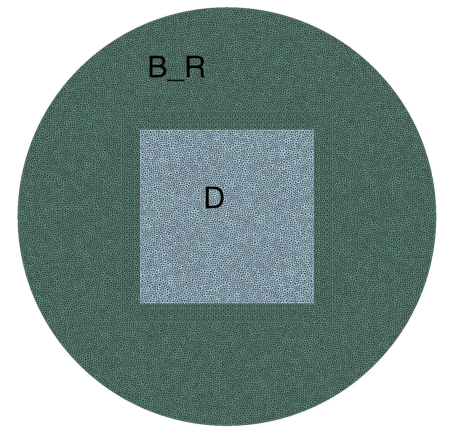
(a) Mesh with domains

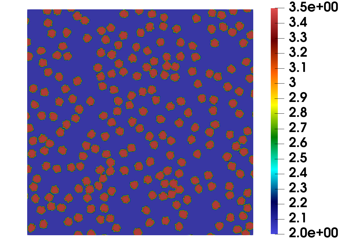
(b) Realization of $a_{\varepsilon}$ with $\varepsilon=0.09$ in $D$

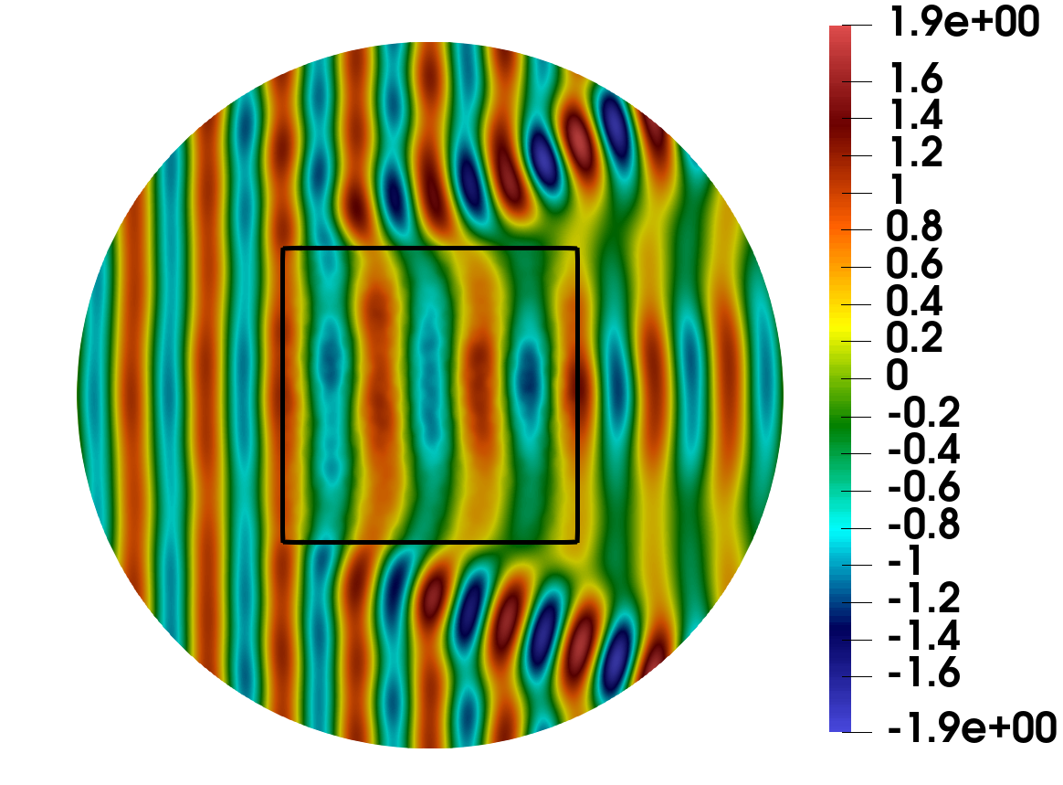
(c) Solution $u_{\varepsilon}$ with $\varepsilon=0.09$

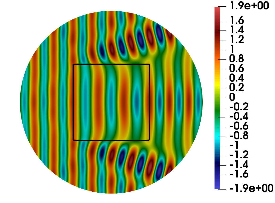
(d) Solution $u_{0}$

Figure 2: (a) Mesh, (b) $a_{\varepsilon}$ for a realization of $S$ with $\varepsilon=0.09$, (c) corresponding $u_{\varepsilon}$ and (d) homogenized solution $u_{0}$ for an incident plane wave along $(1,0)$

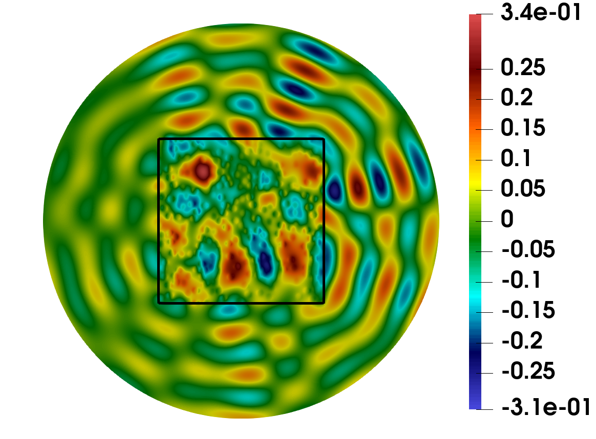
(a) $u_{\varepsilon}-u_{0}$ for the realization of $S$ in Figure 2(b) ($\varepsilon=0.09$)

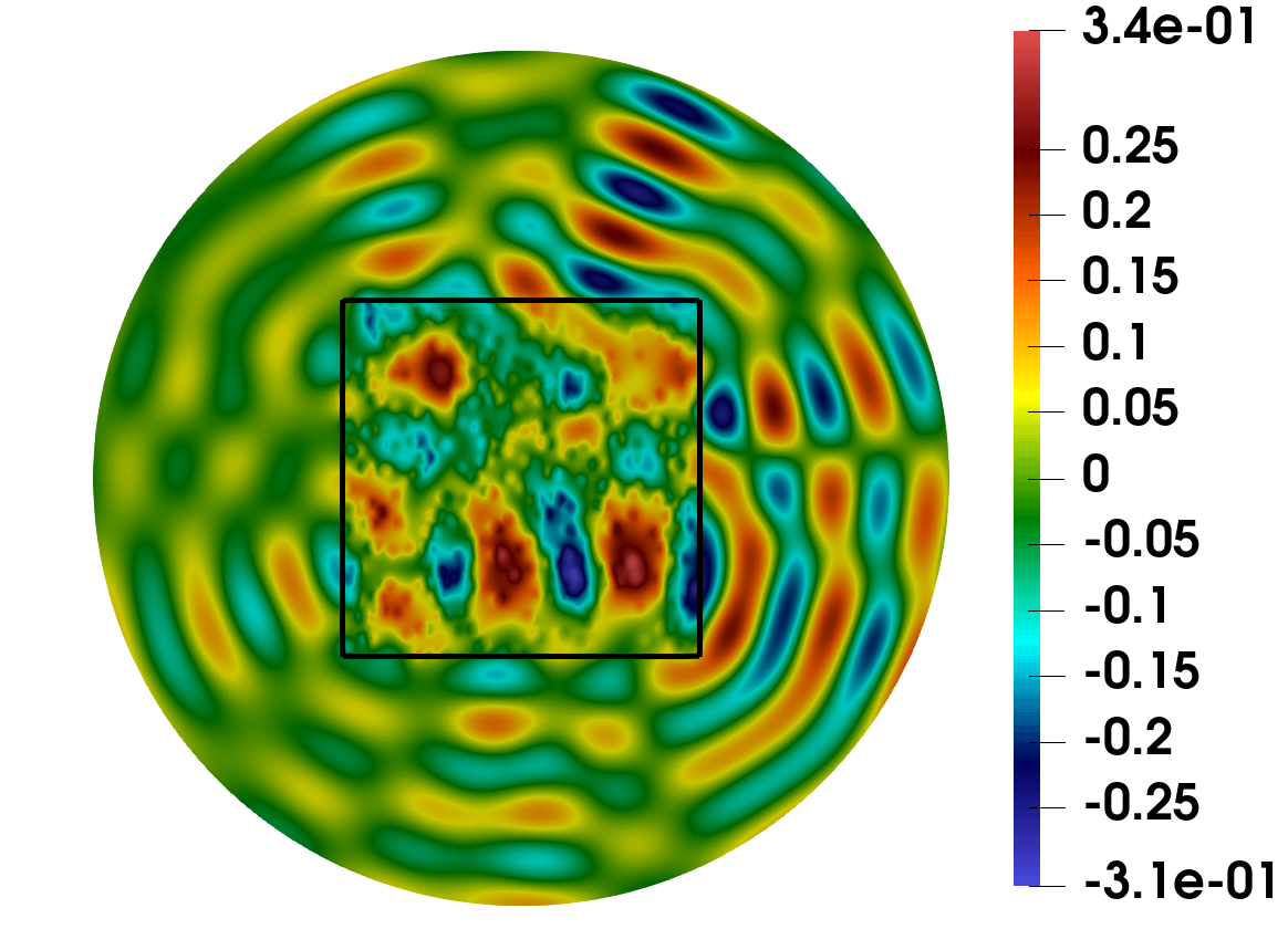
(b) $\mathcal{U}_{1}$ for the realization of $S$ in Figure 2(b) ($\varepsilon=0.09$)

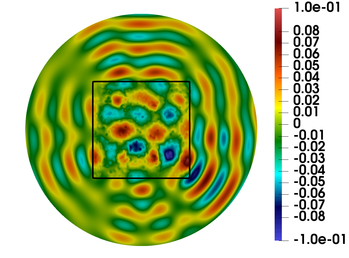
(c) $u_{\varepsilon}-u_{0}-\mathcal{U}_{1}$ for the realization of $S$ in Figure 2(b) ($\varepsilon=0.09$)

Figure 3: For the realization $S$ shown in Figure 2(b), (a) error term $u_{\varepsilon}-u_{0}$, (b) correction term $\mathcal{U}_{1}$, (c) error term term $u_{\varepsilon}-u_{0}-\mathcal{U}_{1}$

The Monte-Carlo process to compute the average error is done with $30$ realizations on Figure 4.
One can see on Figure 4, that the expected error decay of order $\varepsilon^{\frac{d+1}{2}}\mu_{d}(\frac{1}{\varepsilon})^{\frac{1}{2}}=\varepsilon^{\frac{3}{2}}|\log(\varepsilon)|^{\frac{1}{2}}$ in Theorem 10 is obtained. For values of $\varepsilon$ of order $0.1$, the asymptotic expansion $u_{0}+\varepsilon\mathcal{U}_{1}$ is already a very good approximation of the field $u_{\varepsilon}$.

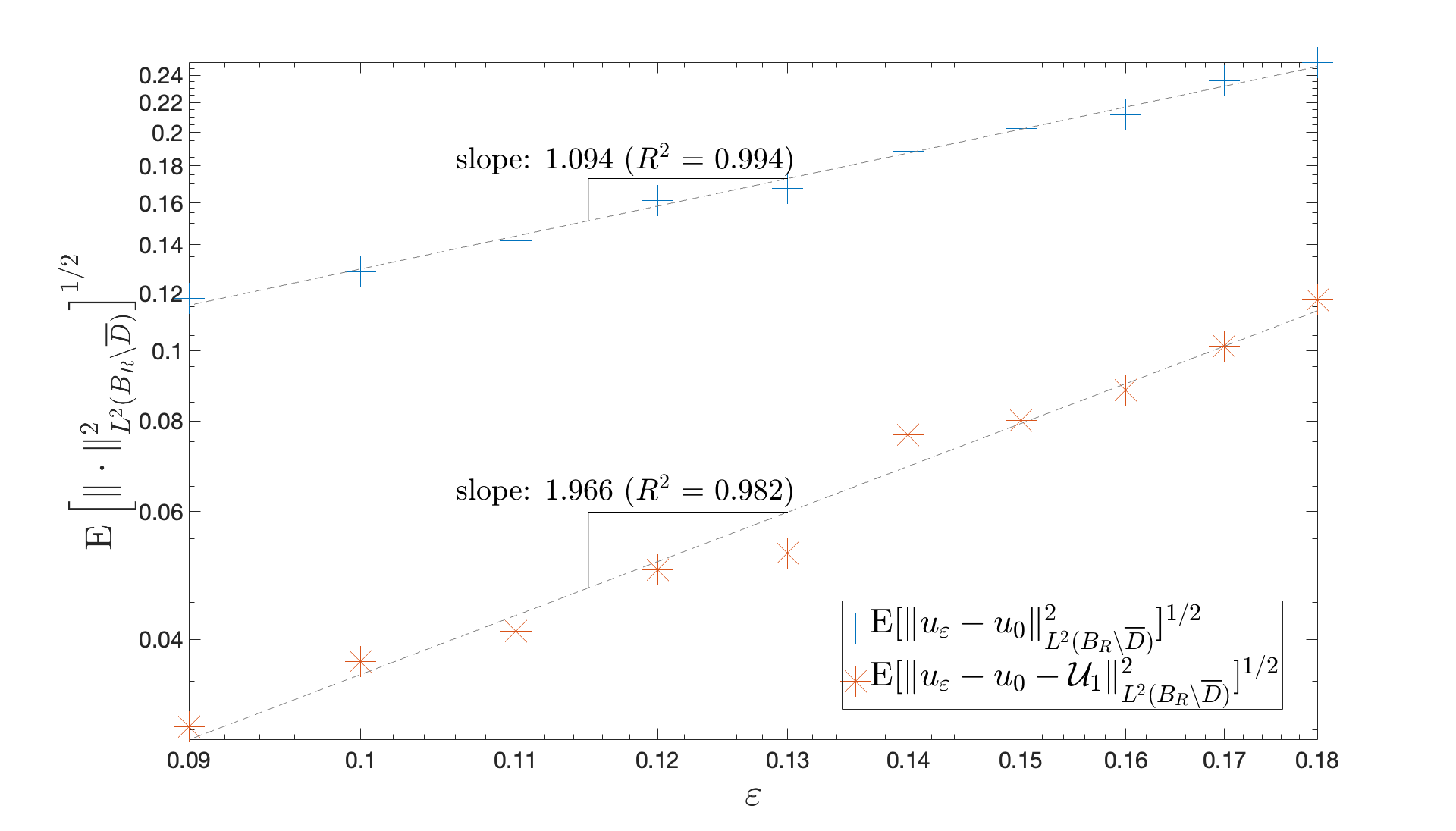
Figure 4: Error decay and linear regression

Appendix A Well-posedness of the scattering problem and $H^{s}$-regularity

We show in this appendix that the scattering problems are well-posed in $H^{1}(B_{R}\setminus\overline{D})\times H^{1}(D)$ with a control of $u_{\varepsilon}$ that is independent on $\varepsilon$ and the randomness. To do so, we suppose that the bilinear form associated to (12) is coercive. Finally, we prove that $u_{0}$ can be more regular than $H^{1}$ under regularity assumptions on the boundary of $D$ and the source terms. The coercivity of the bilinear form is not a restrictive hypothesis. It can be shown for example under either one of the following sufficient conditions [19]

1. $\Im k>0$

2. $kR$ is small enough (low frequency).

Proposition 14 (Uniform stability under coercivity assumption).

Let $D\subset\mathbb{R}^{d}$ be a non-empty, open, and bounded set having $\mathcal{C}^{2}$- boundary $\partial D$ such that the exterior domain $\mathbb{R}^{d}\setminus\overline{D}$ is connected. Let $A:\overline{D}\mapsto\mathbb{C}^{d\times d}$ and $n:\overline{D}\mapsto\mathbb{C}$. We suppose that $A(x)$, $x\in\overline{D}$, is a definite positive matrix that satisfies, $\xi\cdot A\xi\geq\Lambda_{A}^{-}|\xi|^{2}$ and $|A\xi|\leq\Lambda_{A}^{+}|\xi|$ for all $\xi\in\mathbb{C}^{3}$ and $x\in D$, and that $\Lambda_{n}^{+}\geq n\geq\Lambda_{n}^{-}>0$ where $\Lambda_{A}^{+}$, $\Lambda_{A}^{-}$, $\Lambda_{n}^{+}$, $\Lambda_{n}^{-}$ are positive constants.
Let $f\in L^{2}(D)$, $g\in H^{\frac{1}{2}}(\partial D)$ and $h\in H^{-\frac{1}{2}}(\partial D)$. Then, there exists a unique $u\in H^{1}(B_{R}\setminus\overline{D})\times H^{1}(D)$ solution of the transmission problem

$$\left\{\begin{aligned} &-\Delta u^{-}-k^{2}n_{0}u^{-}=0&&\textrm{in}\,B_{R}\setminus\overline{D},\\ &-\nabla\cdot\left(A\nabla u^{+}\right)-k^{2}nu^{+}=f&&\textrm{in}\,D,\\ &u^{-}-u^{+}=g&&\textrm{on}\,\partial D,\\ &\nabla u^{-}\cdot\nu-A\nabla u^{+}\cdot\nu=h&&\textrm{on}\,\partial D,\\ &\nabla u\cdot\nu=\Lambda(u)&&\textrm{on}\,\partial B_{R},\\ \end{aligned}\right.$$ (136)

which satisfies the uniform control:

$$\left\|u\right\|_{H^{1}(B_{R}\setminus\overline{D})}+\left\|u\right\|_{H^{1}(D)}\lesssim\left\|f\right\|_{L^{2}(D)}+\left\|g\right\|_{H^{\frac{1}{2}}(\partial D)}+\left\|h\right\|_{H^{-\frac{1}{2}}(\partial D)}.$$ (137)

We also need a regularity result on the homogenized solution $u_{0}$ that we recall here.

Proposition 15 ($H^{s}$- regularity for the transmission problem).

Let $s\geq 2$. Let $D$ be a bounded domain of class $\mathcal{C}^{s}$. If $A,n\in\mathcal{C}^{s-2}(\overline{D})$, $f\in H^{s-2}(D)$ $g\in H^{s-{\frac{1}{2}}}(\partial D)$ and $h\in H^{s-{\frac{3}{2}}}(\partial D)$, then the unique solution $u\in H^{1}(D)\times H^{1}(B_{R}\setminus\overline{D})$ of (136) belongs to $H^{s}(D)\times H^{s}(B_{R}\setminus\overline{D})$. Moreover the following estimate holds:

$$\left\|u\right\|_{H^{s}(B_{R}\setminus\overline{D})}+\left\|u\right\|_{H^{s}(D)}\lesssim\left\|f\right\|_{H^{s-2}(D)}+\left\|g\right\|_{H^{s-\frac{1}{2}}(\partial D)}+\left\|h\right\|_{H^{s-\frac{3}{2}}(\partial D)}.$$ (138)

Proof.

We rely on elliptic regularity results proved in [48] to establish our result. We first prove that $u$ belongs to $H^{2}(D)$. Since $u\in H^{1}(D)$, its trace on $\partial D$ belongs to $H^{\frac{1}{2}}(\partial D)$. Let $\widetilde{u}\in H^{1}(D)$ be the unique solution of

$$\left\{\begin{aligned} &-\nabla\cdot\left(A\nabla\widetilde{u}\right)-k^{2}n\widetilde{u}=0&&\textrm{in}\,D,\\ &\widetilde{u}=u&&\textrm{on}\,\partial D.\\ \end{aligned}\right.$$ (139)

Then $\widetilde{u}$ satisfies the hypotheses of [48, Theorem 3.4.1] and therefore $\widetilde{u}$ is in $H^{2}(D)$.
By uniqueness of the solution of (139), we also have:

$$\widetilde{u}=u\quad\textrm{in}\,D.$$

Therefore $u\in H^{2}(D)$. Using the same reasoning in $B_{R}\setminus\overline{D}$ with a Dirichlet-to-Neumann operator on the boundary of $B_{R}$, one concludes that $u\in H^{2}(B_{R}\setminus\overline{D})$.
Similarly we can now apply [48, Theorem 2.3.2 (ii)] to show that $u$ belongs in fact to $H^{s}(D)\times H^{s}(B_{R}\setminus\overline{D})$ and get the estimate. ∎

Appendix B Qualitative homogenization

We detail here the proof of the convergence of $u_{\varepsilon}$ towards $u_{0}$ strongly in $L^{2}(B_{R})$ and weakly in $H^{1}(B_{R})$ by the method of oscillating test functions.

Proposition 16 (Homogenization of the scattering problem in $H^{1}(B_{R})$).

Let $u_{\varepsilon}$ be the a.s. unique solution in $H^{1}(B_{R})$ of (12) and $u_{0}\in H^{1}(B_{R})$ be the solution of (13). Then we have the following convergence results as $\varepsilon$ goes to $0$

$$\left\{\begin{aligned} &u_{\varepsilon}\xrightarrow{L^{2}(B_{R})}u_{0},\\ &\nabla u_{\varepsilon}\xrightharpoonup{L^{2}(B_{R})}\nabla u_{0},\\ &a_{\varepsilon}\nabla u_{\varepsilon}\xrightharpoonup{L^{2}(B_{R})}a^{hom}\nabla u_{0}.\end{aligned}\right.$$ (140)

Here, we extend $a^{hom}$ by $I$ in $B_{R}\setminus\overline{D}$.

Proof.

Since a.s. $u_{\varepsilon}$ is uniformly bounded in $H^{1}(B_{R})$ independently of $\varepsilon$, by Rellich-Kondrachov theorem, we can extract a subsequence, still denoted $u_{\varepsilon}$ such that

$$u_{\varepsilon}\xrightharpoonup{H^{1}(B_{R})}u,$$ (141)

for a certain $u\in H^{1}(B_{R})$. By Rellich’s theorem we have then $u_{\varepsilon}\xlongrightarrow{L^{2}(B_{R})}u$. Similarly thanks to the uniform ellipticity of $a$, we have:

$$\left\|a_{\varepsilon}\nabla u_{\varepsilon}\right\|_{L^{2}(B_{R})}\leq\Lambda_{a}\left\|\nabla u_{\varepsilon}\right\|_{L^{2}(B_{R})}\lesssim\left\|u^{inc}\right\|_{H^{1}(B_{R})}.$$

Therefore we can also extract a subsequence of $a_{\varepsilon}\nabla u_{\varepsilon}$ such that

$$a_{\varepsilon}\nabla u_{\varepsilon}\xrightharpoonup{L^{2}(B_{R})}F^{\star}$$

for some $F^{\star}\in L^{2}(B_{R})$.
We show that $u=u_{0}$ and $F^{\star}=a^{hom}\nabla u_{0}$.
By Birkhoff’s ergodic theorem and the strong convergence of $u_{\varepsilon}$ to $u$ in $L^{2}(D)$, we have that

$$n_{\varepsilon}u_{\varepsilon}\xrightharpoonup{L^{2}(B_{R})}\mathbb{E}[n]u=n^{hom}u.$$

Furthermore, the $DtN$ operator is continuous from $H^{\frac{1}{2}}(\partial B_{R})$ to $H^{-\frac{1}{2}}(\partial B_{R})$ and the trace operator is continuous from $H^{1}(B_{R})$ to $H^{\frac{1}{2}}(\partial B_{R})$. Thus

$$\Lambda(u_{\varepsilon})\xrightharpoonup{H^{-\frac{1}{2}}(\partial B_{R})}\Lambda(u).$$

By passing to the limit inside the variational formulation of (12) for $u_{\varepsilon}$, one finds that, for all $v\in H^{1}(B_{R})$,

$$\begin{split}\int_{D}F^{\star}\cdot\nabla\overline{v}-&k^{2}n^{hom}u\overline{v}+\int_{B_{R}\setminus\overline{D}}F^{\star}\cdot\nabla\overline{v}-k^{2}n_{0}u\overline{v}\\ &\hskip 19.91684pt-\left\langle\Lambda(u),v\right\rangle_{H^{-\frac{1}{2}}(\partial B_{R}),H^{\frac{1}{2}}(\partial B_{R})}=\left\langle\Lambda(u^{inc}),v\right\rangle_{H^{-\frac{1}{2}}(\partial B_{R}),H^{\frac{1}{2}}(\partial B_{R})}.\end{split}$$ (142)

For $i\in[\![1,d]\!]$, let $\psi_{i}\in H^{1}_{loc}(\mathbb{R}^{d})$ be the adjoint corrector satisfying

$$-\nabla\cdot a^{*}(\nabla\psi_{i}+e_{i})=0\quad\textrm{in }\mathcal{D}^{\prime}(\mathbb{R}^{d}),$$ (143)

with the anchoring condition $\frac{1}{|\square_{0}|}\int_{\square_{0}}\psi_{i}=0$.
Moreover, $\nabla\psi_{i}$ is stationary, verifies $\mathbb{E}[\nabla\psi_{i}]=0$ and admits finite second order moment. Now for all $x\in\mathbb{R}^{d}$, let

$$\alpha_{i}(x):=x_{i}+\psi_{i}(x),$$

and

$$\alpha_{i}^{\varepsilon}(x):=\varepsilon\alpha_{i}(\frac{x}{\varepsilon})=x_{i}+\varepsilon\psi_{i}(\frac{x}{\varepsilon}).$$

Thanks to the sublinearity of $\psi_{i}$, $\alpha_{i}^{\varepsilon}\xrightarrow{L^{2}(B_{R})}x_{i}$. Moreover by Birkhoff’s theorem $\nabla\alpha_{i}^{\varepsilon}\xrightharpoonup{L^{2}(B_{R})}e_{i}$. Thus

$$\alpha_{i}^{\varepsilon}\xrightharpoonup{H^{1}(B_{R})}x_{i}.$$

Similarly by Birkhoff’s theorem, $a_{\varepsilon}^{*}\nabla\alpha_{i}^{\varepsilon}\xrightharpoonup{L^{2}(B_{R})}\mathbb{E}[a^{*}\nabla\alpha_{i}]=\mathbb{E}[a^{*}(e_{i}+\nabla\psi_{i})]$.
Moreover, since $\mathbb{E}[\nabla\phi_{j}\cdot a^{*}(e_{i}+\nabla\psi_{i})]=\mathbb{E}[\nabla\psi_{i}\cdot a(e_{j}+\nabla\phi_{j})]=0$ for $i,j\in[\![1,d]\!],$

$$\begin{split}\mathbb{E}[e_{j}\cdot a^{*}\nabla\alpha_{i}]&=\mathbb{E}[(e_{j}+\nabla\phi_{j})\cdot a^{*}(e_{i}+\nabla\psi_{i})\\ &=\mathbb{E}[a(e_{j}+\nabla\phi_{j})\cdot e_{i}\\ &=a^{hom}_{ji}=e_{i}\cdot a^{hom}e_{j}.\end{split}$$ (144)

For $\zeta\in C_{c}^{\infty}(B_{R})$ consider the variational formulation of the problem solved by $u_{\varepsilon}$ with the test function $\zeta\alpha^{\varepsilon}_{i}$,

$$\begin{split}0&=\int_{B_{R}}a_{\varepsilon}\nabla u_{\varepsilon}\cdot\nabla(\overline{\zeta}\alpha^{\varepsilon}_{i})-k^{2}n_{\varepsilon}u_{\varepsilon}\overline{\zeta}\alpha^{\varepsilon}_{i}\\ &=\int_{B_{R}}a_{\varepsilon}\nabla u_{\varepsilon}\cdot(\nabla\overline{\zeta})\alpha^{\varepsilon}_{i}-(\nabla\overline{\zeta})u_{\varepsilon}\cdot a_{\varepsilon}^{*}\nabla\alpha^{\varepsilon}_{i}-k^{2}n_{\varepsilon}u_{\varepsilon}\overline{\zeta}\alpha^{\varepsilon}_{i}.\\ \end{split}$$ (145)

Then, by passing to the limit

$$\begin{split}\int_{D}F^{\star}\cdot(\nabla\zeta)x_{i}-&(\nabla\zeta)u\cdot(a^{hom})^{*}e_{i}-k^{2}n^{hom}u\zeta x_{i}\\ &+\int_{B_{R}\setminus\overline{D}}F^{\star}\cdot(\nabla\zeta)x_{i}-a^{hom}(\nabla\zeta)u\cdot e_{i}-k^{2}n_{0}u\zeta x_{i}=0.\\ \end{split}$$ (146)

Moreover by (142)

$$\begin{split}\int_{B_{R}}F^{\star}\cdot(\nabla\overline{\zeta})x_{i}&=\int_{B_{R}}F^{\star}\cdot\nabla(\overline{\zeta}x_{i})-F\cdot\overline{\zeta}e_{i}\\ &=\int_{B_{R}\setminus\overline{D}}k^{2}n_{0}u\overline{\zeta}x_{i}+\int_{D}k^{2}n^{hom}u\overline{\zeta}x_{i}-\int_{B_{R}}F^{\star}\cdot\overline{\zeta}e_{i}.\end{split}$$ (147)

Since $\zeta u\in H^{1}_{0}(B_{R})$, an integration by parts yields

$$\begin{split}\int_{B_{R}}a^{hom}(\nabla\overline{\zeta})u\cdot e_{i}=\int_{B_{R}}-a^{hom}\nabla u\cdot\overline{\zeta}e_{i}\end{split}$$ (148)

which yields that for any $\zeta\in C^{\infty}_{c}(B_{R})$ and for any $i\in[\![1,d]\!]$,

$$\int_{B_{R}}\overline{\zeta}e_{i}\cdot(a^{hom}\nabla u-F^{\star})=0.$$ (149)

This implies that a.s. $F^{\star}=a^{hom}\nabla u$ in $\mathcal{D}^{\prime}(B_{R})$, thus in $L^{2}(B_{R})$.
Finally, (142) can then be rewritten as

$$\begin{split}\int_{B_{R}}a^{hom}\nabla u\cdot\nabla\overline{v}-k^{2}n^{hom}u\overline{v}-\left\langle\Lambda(u),v\right\rangle_{H^{-\frac{1}{2}}(\partial B_{R}),H^{\frac{1}{2}}(\partial B_{R})}=\\ &\left\langle\Lambda(u^{inc}),v\right\rangle_{H^{-\frac{1}{2}}(\partial B_{R}),H^{\frac{1}{2}}(\partial B_{R})}.\end{split}$$ (150)

We get $u=u_{0}$. Moreover by uniqueness of the limit, we proved convergence of $u_{\varepsilon}$ and $a_{\varepsilon}\nabla u_{\varepsilon}$ and not just of a subsequence. ∎

Appendix C Homogenization with a less regular solution

In Section 3 Proposition 7, we proved an error estimate for the two-scale expansion when ${u_{0}}_{|_{D}}\in W^{2,\infty}(D)$. This result still holds for less regular $u_{0}$ as stated in Proposition 18.
As done in [14], we consider an extension of ${u_{0}}_{|_{D}}$ that we denote $\widehat{u_{0}}\in W^{1+\alpha,p}(\mathbb{R}^{d})$. $\widehat{u_{0}}$ is defined through the Sobolev extension theorem stated below.

Lemma 17 (Sobolev extension theorem [14, Proposition B.14]).

Let $D$ be a bounded Lipschitz domain, $\alpha\in(0,\infty)$ and $p\in(1,\infty)$. The restriction operator ${W^{\alpha,p}(\mathbb{R}^{d})\rightarrow W^{\alpha,p}(D)}$ has a bounded linear right inverse. That is, there exists a linear operator

$$\text{Ext}:W^{\alpha,p}(D)\rightarrow W^{\alpha,p}(\mathbb{R}^{d}),$$

such that, for every $u\in W^{\alpha,p}(D)$,

$$\text{Ext}(u)=u~{}a.e.~{}\text{ in }D,$$

and

$$\left\|\text{Ext}(u)\right\|_{W^{\alpha,p}(\mathbb{R}^{d})}\lesssim\left\|u\right\|_{W^{\alpha,p}(D)}.$$

We derive a convergence rate of $u_{\varepsilon}$ towards the two-scale expansion when ${{u_{0}}_{|_{D}}\in W^{1+\alpha,p}(D)}$.

Proposition 18 ($H^{1}$- convergence of the two-scale expansion for ${{u_{0}}_{|_{D}}\in W^{1+\alpha,p}(D)}$).

For $p\in(2,\infty]$, $\alpha\in(\frac{1}{p},1]$, suppose that $u_{0}\in H^{1}(B_{R})$ such that ${{u_{0}}_{|_{D}}\in W^{1+\alpha,p}(D)}$ then

$$\begin{split}\left\|u_{\varepsilon}-\right.&\left.u_{0}\right\|_{H^{1}(B_{R}\setminus\overline{D})}+\left\|u_{\varepsilon}-u_{0}-\widehat{u_{1,\varepsilon}}\right\|_{H^{1}(D)}\lesssim\varepsilon^{\frac{1}{2}}\mu_{d}(\frac{1}{\varepsilon})^{\frac{1}{2}}\widehat{\chi_{\varepsilon,p}}\left\|u_{0}\right\|_{W^{1+\alpha,p}(D)},\end{split}$$ (151)

where $\widehat{u}_{1,\varepsilon}$ is defined by

$$\widehat{u}_{1,\varepsilon}(x):=\mathbbm{1}_{D}(x)\sum_{i=1}^{d}\phi_{i}\biggl{(}\frac{x}{\varepsilon}\biggr{)}\partial_{i}\widehat{u_{0}}*\xi_{\varepsilon}(x)\quad\textrm{for }x\in B_{R},$$

with the standard mollifier $\xi_{\varepsilon}$ defined by

$$\xi_{\varepsilon}(x):=\varepsilon^{-d}\left\{\begin{array}[]{ll}\vspace{0.2cm}\displaystyle c_{d}\exp(-\frac{1}{1-|\frac{x}{\varepsilon}|^{2}})&\textrm{for}\,\,|\frac{x}{\varepsilon}|<1,\\ \vspace{0.2cm}\displaystyle 0&\textrm{for }\,\,|\frac{x}{\varepsilon}|\geq 1,\\ \end{array}\right.$$ (152)

and $c_{d}$ is such that

$$\int_{\mathbb{R}^{d}}\xi_{\varepsilon}(x)\mathrm{d}x=1.$$

Here $\widehat{\chi_{\varepsilon,p}}$ denotes a random variable satisfying the stochastic integrability (38).

In order to prove the previous theorem, we introduce the boundary corrector and start by proving the result with the boundary corrector.

Proposition 19 ($H^{1}$- convergence of the two-scale expansion with the boundary corrector for ${{u_{0}}_{|_{D}}\in W^{1+\alpha,p}(D)}$).

For $p\in(2,\infty]$, $\alpha\in(0,1]$, suppose that $u_{0}\in H^{1}(B_{R})$ such that ${{u_{0}}_{|_{D}}\in W^{1+\alpha,p}(D)}$ then

$$\left\|u_{\varepsilon}-u_{0}-\widehat{u}_{1,\varepsilon}-\widehat{v_{\varepsilon}}\right\|_{H^{1}(B_{R})}\lesssim\varepsilon^{\alpha}\mu_{d}(\frac{1}{\varepsilon})\chi_{\varepsilon,p}\left\|u_{0}\right\|_{W^{1+\alpha,p}(D)},$$ (153)

where the boundary corrector ${\widehat{v_{\varepsilon}}\in H^{1}(B_{R}\setminus\overline{D})\times H^{1}(D)}$ is the solution of

$$\left\{\begin{aligned} &-\Delta\widehat{v_{\varepsilon}}-k^{2}\widehat{v_{\varepsilon}}=0&&\textrm{in}\,B_{R}\setminus\overline{D},\\ &-\nabla\cdot a_{\varepsilon}\nabla\widehat{v_{\varepsilon}}-k^{2}n_{\varepsilon}\widehat{v_{\varepsilon}}=0&&\textrm{in}\,D,\\ &\widehat{v_{\varepsilon}}^{-}-\widehat{v_{\varepsilon}}^{+}=\varepsilon\widehat{u}_{1,\varepsilon}&&\textrm{on}\,\partial D,\\ &\nabla\widehat{v_{\varepsilon}}^{-}\cdot\nu-a_{\varepsilon}\nabla\widehat{v_{\varepsilon}}^{+}\cdot\nu=\varepsilon\left(\nabla\cdot(\sigma_{i}^{\varepsilon}\partial_{i}\widehat{u_{0}}*\xi_{\varepsilon})^{+}\right)\cdot\nu\\ &\hskip 142.26378pt-k^{2}\varepsilon(\beta^{\varepsilon}\widehat{u_{0}}*\xi_{\varepsilon})^{+}\cdot\nu&&\textrm{on}\,\partial D,\\ &\nabla\widehat{v_{\varepsilon}}\cdot\nu=\Lambda(\widehat{v_{\varepsilon}})&&\textrm{on}\,\partial B_{R}.\end{aligned}\right.$$ (154)

$\chi_{\varepsilon,p}$ is a random variable defined as

$$\chi_{\varepsilon,p}:=\left(\varepsilon^{d}\sum_{z\in P_{\varepsilon}(D)}\mathcal{C}(z)^{\frac{2p}{p-2}}\right)^{\frac{p-2}{2p}},$$ (155)

with $\mathcal{C}$ denoting the constant in Proposition 5. Moreover $\chi_{\varepsilon,p}$ satisfies the stochastic integrability (38).

Both results of Proposition 18 and Proposition 19 were established for the Poisson equation in a bounded domain with Dirichlet or Neumann condition in [14, Chapter 6]. The proofs below use similar arguments as the ones developed in [14].

Proof of Proposition 19.

We denote $\widehat{Z_{\varepsilon}}:=u_{\varepsilon}-u_{0}-\varepsilon\widehat{u_{1,\varepsilon}}$.
As in Proposition 6, the boundary layer $\widehat{v_{\varepsilon}}$ solution of (154) is constructed such that $\widehat{Z_{\varepsilon}}-\widehat{v_{\varepsilon}}$ is the unique solution in $H^{1}(B_{R})$ of

$$\left\{\begin{aligned} &-\nabla\cdot a_{\varepsilon}\nabla(\widehat{Z_{\varepsilon}}-\widehat{v_{\varepsilon}})-k^{2}n_{\varepsilon}(\widehat{Z_{\varepsilon}}-\widehat{v_{\varepsilon}})=\nabla\cdot\widehat{F_{\varepsilon}}+k^{2}\widehat{G_{\varepsilon}}&&\textrm{in}\,B_{R},\\ &\nabla(\widehat{Z_{\varepsilon}}-\widehat{v_{\varepsilon}})\cdot\nu=\Lambda(\widehat{Z_{\varepsilon}}-\widehat{v_{\varepsilon}})&&\textrm{on}\,\partial B_{R},\\ \end{aligned}\right.$$ (156)

where $\widehat{F_{\varepsilon}}$ and $\widehat{G_{\varepsilon}}$ are defined by

$$\widehat{F_{\varepsilon}}:=\varepsilon(a_{\varepsilon}\phi_{i}^{\varepsilon}-\sigma_{i}^{\varepsilon})\nabla(\partial_{i}\widehat{u_{0}}*\xi_{\varepsilon})+(a_{\varepsilon}-a^{hom})\nabla(\widehat{u_{0}}*\xi_{\varepsilon}-u_{0})+\varepsilon k^{2}\beta^{\varepsilon}\widehat{u_{0}}*\xi_{\varepsilon},$$ (157)

and

$$\widehat{G_{\varepsilon}}:=\varepsilon\left((n_{\varepsilon}\phi_{i}^{\varepsilon}-\beta_{i}^{\varepsilon})\partial_{i}\widehat{u_{0}}*\xi_{\varepsilon}\right)+(n_{\varepsilon}-n^{hom})(u_{0}-\widehat{u_{0}}*\xi_{\varepsilon}).$$ (158)

Moreover, $\widehat{Z_{\varepsilon}}-\widehat{v_{\varepsilon}}$ verifies a.s.

$$\left\|\widehat{Z_{\varepsilon}}-\widehat{v_{\varepsilon}}\right\|_{H^{1}(B_{R})}\lesssim\left\|\widehat{F_{\varepsilon}}\right\|_{L^{2}(D)}+\left\|\widehat{G_{\varepsilon}}\right\|_{L^{2}(D)}.$$ (159)

To prove (151), we hence need to prove that

$$\left\|\widehat{F_{\varepsilon}}\right\|_{L^{2}(D)}+\left\|\widehat{G_{\varepsilon}}\right\|_{L^{2}(D)}\lesssim\varepsilon^{\alpha}\mu_{d}(\frac{1}{\varepsilon})\chi_{\varepsilon,p}\left\|u_{0}\right\|_{W^{1+\alpha,p}(D)}.$$

By the triangle inequality, we immediately get

$$\begin{split}&\left\|\widehat{F_{\varepsilon}}\right\|_{L^{2}(D)}+\left\|\widehat{G_{\varepsilon}}\right\|_{L^{2}(D)}\\ &\hskip 28.45274pt\lesssim\varepsilon\left\||\phi^{\varepsilon}-\sigma^{\varepsilon}||\nabla\nabla\widehat{u_{0}}*\xi_{\varepsilon}|\right\|_{L^{2}(D)}+\varepsilon\left\||\beta^{\varepsilon}||\widehat{u_{0}}*\xi_{\varepsilon}|\right\|_{L^{2}(D)}\\ &+\varepsilon\left\||\phi^{\varepsilon}-\beta^{\varepsilon}|\nabla\widehat{u_{0}}*\xi_{\varepsilon}\right\|_{L^{2}(D)}+\left\|\nabla(\widehat{u_{0}}*\xi_{\varepsilon}-u_{0})\right\|_{L^{2}(D)}+\left\|\widehat{u_{0}}*\xi_{\varepsilon}-u_{0}\right\|_{L^{2}(D)}.\end{split}$$ (160)

It remains to estimate these five terms.
We recall a useful Lemma, proved in [14], which allows us to estimate the three first terms of (160).

Lemma 20 ([14, Lemma 6.8]).

Fix $\alpha\in(0,1]$ and $p\in(2,\infty)$. Let $f\in L^{2}(D+2\varepsilon\square_{0})$, $g\in L^{p}(D+2\varepsilon\square_{0})$ and its Sobolev extension $\widehat{g}\in L^{p}(\mathbb{R}^{d})$. Then

$$\left\|f|\widehat{g}*\xi_{\varepsilon}|\right\|_{L^{2}(D)}\lesssim\left(\varepsilon^{d}\sum_{z\in P_{\varepsilon}(D)}\left\|f\right\|_{\underline{L}^{2}(z+2\varepsilon\square_{0})}^{\frac{2p}{p-2}}\right)^{\frac{p-2}{2p}}\left\|g\right\|_{L^{p}(D+2\varepsilon\square_{0})},$$ (161)

where $\left\|f\right\|_{\underline{L}^{2}(z+2\varepsilon\square_{0})}:=\left\|f\right\|_{\underline{L}^{2}(z+2\varepsilon\square_{0})}:=\left(\fint_{z+2\varepsilon\square_{0}}|f|^{2}\right)^{\frac{1}{2}}$.
Moreover, if $g\in W^{\alpha,p}(D+2\varepsilon\square_{0})$, then

$$\left\|f|\nabla(\widehat{g}*\xi_{\varepsilon})|\right\|_{L^{2}(D)}\lesssim\varepsilon^{\alpha-1}\left(\varepsilon^{d}\sum_{z\in P_{\varepsilon}(D)}\left\|f\right\|_{\underline{L}^{2}(z+2\varepsilon\square_{0})}^{\frac{2p}{p-2}}\right)^{\frac{p-2}{2p}}\left\|g\right\|_{W^{\alpha,p}(D+2\varepsilon\square_{0})}.$$ (162)

Now, using (162), with $f=\phi^{\varepsilon}$ and $g=\nabla\widehat{u_{0}}$ and the corrector estimate of Proposition 5, we obtain

$$\begin{split}\left\||\phi^{\varepsilon}|\right.&\left.|\nabla(\nabla\widehat{u_{0}}*\xi_{\varepsilon})|\right\|_{L^{2}(D)}\\ &\lesssim\varepsilon^{\alpha-1}\left(\varepsilon^{d}\sum_{z\in P_{\varepsilon}(D)}\left\|\phi^{\varepsilon}\right\|_{\underline{L}^{2}(z+2\varepsilon\square_{0}))}^{\frac{2p}{p-2}}\right)^{\frac{p-2}{2p}}\left\|\nabla\widehat{u_{0}}\right\|_{W^{\alpha,p}(D+2\varepsilon\square_{0})}\\ &\lesssim\varepsilon^{\alpha-1}\left(\varepsilon^{d}\sum_{z\in P_{\varepsilon}(D)}\left\|\phi\right\|_{\underline{L}^{2}(2\square_{0})}^{\frac{2p}{p-2}}\right)^{\frac{p-2}{2p}}\left\|\nabla u_{0}\right\|_{W^{\alpha,p}(D)}\\ &\lesssim\varepsilon^{\alpha-1}\mu_{d}(\frac{1}{\varepsilon})\left(\varepsilon^{d}\sum_{z\in P_{\varepsilon}(D)}\mathcal{C}(z)^{\frac{2p}{p-2}}\right)^{\frac{p-2}{2p}}\left\|\nabla u_{0}\right\|_{W^{\alpha,p}(D)}.\end{split}$$ (163)

Similarly, with $f=\phi^{\varepsilon}-\beta^{\varepsilon}$ and $g=\widehat{u_{0}}$,

$$\left\||\phi^{\varepsilon}-\beta^{\varepsilon}||\nabla\widehat{u_{0}}*\xi_{\varepsilon}|\right\|_{L^{2}(D)}\lesssim\varepsilon^{\alpha-1}\mu_{d}(\frac{1}{\varepsilon})\left(\varepsilon^{d}\sum_{z\in P_{\varepsilon}(D)}\mathcal{C}(z)^{\frac{2p}{p-2}}\right)^{\frac{p-2}{2p}}\left\|u_{0}\right\|_{W^{\alpha,p}(D)}.$$ (164)

Now, using (161) with $f=\beta^{\varepsilon}$ and $g=u_{0}$, we get

$$\left\||\beta^{\varepsilon}||u_{0}*\xi_{\varepsilon}|\right\|_{L^{2}(D)}\lesssim\mu_{d}(\frac{1}{\varepsilon})\left(\varepsilon^{d}\sum_{z\in P_{\varepsilon}(D)}\mathcal{C}(z)^{\frac{2p}{p-2}}\right)^{\frac{p-2}{2p}}\left\|u_{0}\right\|_{L^{p}(D)}.$$ (165)

To estimate the last two terms of (160), we recall another useful lemma.

Lemma 21 ([14, Lemma 6.7]).

Fix $1\leq q\leq p<\infty$ and $0<\alpha\leq 1$. Let ${g\in W^{\alpha,p}(D+2\varepsilon\square_{0})}$ and its Sobolev extension $\widehat{g}\in W^{\alpha,p}(\mathbb{R}^{d})$. Then

$$\left\|g-(\widehat{g}*\xi_{\varepsilon})\right\|_{L^{q}(D)}\lesssim|D|^{\frac{1}{q}-\frac{1}{p}}\varepsilon^{\alpha}\left\|g\right\|_{W^{\alpha,p}(D+2\varepsilon\square_{0})}.$$ (166)

Using this Lemma, with $g=\nabla u_{0}$, $q=2$, and $p>2$, we have

$$\left\|\nabla u_{0}-(\nabla\widehat{u_{0}})*\xi_{\varepsilon}\right\|_{L^{2}(D)}\lesssim\varepsilon^{\alpha}\left\|\nabla\widehat{u_{0}}\right\|_{W^{\alpha,p}(D+2\varepsilon\square_{0})}\lesssim\varepsilon^{\alpha}\left\|u_{0}\right\|_{W^{1+\alpha,p}(D)}$$ (167)

and with $g=u_{0}$ we obtain similarly

$$\left\|u_{0}-\widehat{u_{0}}*\xi_{\varepsilon}\right\|_{L^{2}(D)}\lesssim\varepsilon^{\alpha}\left\|\widehat{u_{0}}\right\|_{W^{\alpha,p}(D+2\varepsilon\square_{0})}\lesssim\varepsilon^{\alpha}\left\|u_{0}\right\|_{W^{\alpha,p}(D)}.$$ (168)

Inserting (163), (164), (165), (167), (168) into (160) gives us (151), concluding the proof of Proposition 6.

∎

By estimating the $H^{1}$-norm of the boundary corrector $\widehat{v_{\varepsilon}}$, we can now prove Proposition 18.

Proof of Proposition 18.

We consider $\widehat{V_{\varepsilon}}:=\widehat{v_{\varepsilon}}-\varepsilon\eta_{\varepsilon}\widehat{u_{1,\varepsilon}}$ the a.s. unique solution in $H^{1}(B_{R})$ of

$$\left\{\begin{aligned} &-\Delta\widehat{V_{\varepsilon}}-k^{2}\widehat{V_{\varepsilon}}=0&&\textrm{in}\,B_{R}\setminus\overline{D},\\ &-\nabla\cdot a_{\varepsilon}\nabla\widehat{V_{\varepsilon}}-k^{2}n_{\varepsilon}\widehat{V_{\varepsilon}}=-\varepsilon\nabla\cdot a_{\varepsilon}\nabla(\eta_{\varepsilon}\widehat{u_{1,\varepsilon}})+\varepsilon k^{2}n_{\varepsilon}\eta_{\varepsilon}\widehat{u_{1,\varepsilon}}&&\textrm{in}\,D,\\ &\nabla\widehat{V_{\varepsilon}}^{-}\cdot\nu-a_{\varepsilon}\nabla\widehat{V_{\varepsilon}}^{+}\cdot\nu=\varepsilon a_{\varepsilon}\nabla(\eta_{\varepsilon}\widehat{u_{1,\varepsilon}})\cdot\nu+\varepsilon\left(\nabla\cdot(\sigma_{i}^{\varepsilon}\partial_{i}\widehat{u_{0}}*\xi_{\varepsilon})^{+}\right)\cdot\nu\\ &\hskip 142.26378pt-k^{2}\varepsilon(\beta^{\varepsilon}\widehat{u_{0}}*\xi_{\varepsilon})^{+}\cdot\nu&&\textrm{on}\,\partial D,\\ &\nabla\widehat{V_{\varepsilon}}\cdot\nu=\Lambda(\widehat{V_{\varepsilon}})&&\textrm{on}\,\partial B_{R}.\\ \end{aligned}\right.$$ (169)

As in the proof of Proposition 7, we estimate $\left\|\widehat{V_{\varepsilon}}\right\|_{H^{1}(B_{R})}$ by writing the variational formulation. For $w\in H^{1}(B_{R})$,

$$\begin{split}\int_{B_{R}}&a_{\varepsilon}\nabla\widehat{V_{\varepsilon}}\cdot\nabla\overline{w}-k^{2}n_{\varepsilon}\widehat{V_{\varepsilon}}\overline{w}-\left\langle\Lambda(\widehat{V_{\varepsilon}}),w\right\rangle_{H^{-\frac{1}{2}}(\partial B_{R}),H^{\frac{1}{2}}(\partial B_{R})}\\ &=\int_{D}-\varepsilon a_{\varepsilon}\nabla(\eta_{\varepsilon}\widehat{u_{1,\varepsilon}})\cdot\nabla\overline{w}+\varepsilon k^{2}n_{\varepsilon}(\eta_{\varepsilon}\widehat{u_{1,\varepsilon}})-\varepsilon\nabla\cdot(\sigma_{i}^{\varepsilon}\eta_{\varepsilon}\partial_{i}\widehat{u_{0}}*\xi_{\varepsilon})\cdot\nabla\overline{w}\\ &\hskip 14.22636pt-k^{2}\varepsilon\nabla\cdot(\beta^{\varepsilon}\widehat{u_{0}}*\xi_{\varepsilon}\eta_{\varepsilon})\overline{w}+k^{2}\varepsilon\beta^{\varepsilon}\widehat{u_{0}}*\xi_{\varepsilon}\eta_{\varepsilon}\cdot\nabla\overline{w}.\end{split}$$ (170)

In particular, by the coercivity of the sesquilinear form, we get

$$\begin{split}\left\|\widehat{v_{\varepsilon}}\right\|_{H^{1}(D)}+\left\|\widehat{v_{\varepsilon}}\right\|_{H^{1}(B_{R}\setminus\overline{D})}&\lesssim\varepsilon\left\|\eta_{\varepsilon}\widehat{u_{1,\varepsilon}}\right\|_{H^{1}(D)}+\varepsilon\left\|\sum_{i=1}^{d}\nabla\cdot(\sigma_{i}^{\varepsilon}\partial_{i}\widehat{u_{0}}*\xi_{\varepsilon}\eta_{\varepsilon})\right\|_{L^{2}(D)}+\\ &\hskip 28.45274pt\varepsilon\left\|\nabla\cdot(\beta^{\varepsilon}\widehat{u_{0}}*\xi_{\varepsilon}\eta_{\varepsilon})\right\|_{L^{2}(D)}+\varepsilon\left\|\beta^{\varepsilon}\widehat{u_{0}}*\xi_{\varepsilon}\eta_{\varepsilon}\right\|_{L^{2}(D)}.\end{split}$$ (171)

Let us now estimate $\left\|\eta_{\varepsilon}\widehat{u_{1,\varepsilon}}\right\|_{H^{1}(D)}=\left\|\eta_{\varepsilon}\phi_{i}^{\varepsilon}\partial_{i}\widehat{u_{0}}*\xi_{\varepsilon}\right\|_{H^{1}(D)}$. The three other terms can then be estimated using similar arguments. First

$$\begin{split}\left\|\nabla(\eta_{\varepsilon}\phi_{i}^{\varepsilon}\partial_{i}\widehat{u_{0}}*\xi_{\varepsilon})\right\|_{L^{2}(D)}&\lesssim\left\|(\nabla\eta_{\varepsilon})\phi_{i}^{\varepsilon}\partial_{i}\widehat{u_{0}}*\xi_{\varepsilon}+\eta_{\varepsilon}\nabla(\phi_{i}^{\varepsilon}\partial_{i}\widehat{u_{0}}*\xi_{\varepsilon})\right\|_{L^{2}(D)}\\ &\lesssim\left\|\left(\frac{1}{\mu_{d}(\frac{1}{\varepsilon})}|\nabla\widehat{u_{0}}*\xi_{\varepsilon}|+\varepsilon|\nabla(\nabla\widehat{u_{0}}*\xi_{\varepsilon})|\right)|\phi^{\varepsilon}|+|\nabla\phi||\nabla\widehat{u_{0}}*\xi_{\varepsilon}|\right\|_{L^{2}(\mathcal{S}_{\eta_{\varepsilon}})}.\end{split}$$ (172)

Eq (161) combined with the bounds on the corrector implies

$$\begin{split}\left\|\frac{1}{\mu_{d}(\frac{1}{\varepsilon})}|\nabla\widehat{u_{0}}*\xi_{\varepsilon}||\phi^{\varepsilon}|\right\|_{L^{2}(\mathcal{S}_{\eta_{\varepsilon}})}&\lesssim\varepsilon^{\frac{p-2}{2p}}\mu_{d}(\frac{1}{\varepsilon})^{\frac{p-2}{2p}-1}\widetilde{\chi_{\varepsilon,p}^{1}}\left\|\nabla\widehat{u_{0}}\right\|_{L^{p}(\mathcal{S}_{\eta_{\varepsilon}}+2\varepsilon\square_{0})}\\ \end{split}$$ (173)

and

$$\begin{split}\biggl{\|}|\nabla\widehat{u_{0}}*\xi_{\varepsilon}||\nabla\phi^{\varepsilon}|\biggr{\|}_{L^{2}(\mathcal{S}_{\eta_{\varepsilon}})}&\lesssim\varepsilon^{\frac{p-2}{2p}}\mu_{d}(\frac{1}{\varepsilon})^{\frac{p-2}{2p}}\widetilde{\chi_{\varepsilon,p}^{2}}\left\|\nabla\widehat{u_{0}}\right\|_{L^{p}(\mathcal{S}_{\eta_{\varepsilon}}+2\varepsilon\square_{0})}\\ \end{split}$$ (174)

where the random variables $\widetilde{\chi_{\varepsilon,p}^{1}}$ and $\widetilde{\chi_{{}_{\varepsilon},p}^{2}}$ are defined as

$$\left\{\begin{aligned} &\widetilde{\chi_{\varepsilon,p}^{1}}:=\left(\frac{\varepsilon^{d}}{\varepsilon\mu_{d}(\frac{1}{\varepsilon})}\sum_{z\in P_{\varepsilon}(\mathcal{S}_{\eta_{\varepsilon}})}\mathcal{C}(z)^{\frac{2p}{p-2}}\right)^{\frac{p-2}{2p}},\\ &\widetilde{\chi_{\varepsilon,p}^{2}}:=\left(\frac{\varepsilon^{d}}{\varepsilon\mu_{d}(\frac{1}{\varepsilon})}\sum_{z\in P_{\varepsilon}(\mathcal{S}_{\eta_{\varepsilon}})}(1+r_{*}(z))^{d\frac{2p}{p-2}}\right)^{\frac{p-2}{2p}}.\end{aligned}\right.$$ (175)

We use the following Lemma to estimate $\left\|\nabla\widehat{u_{0}}\right\|_{L^{p}(\mathcal{S}_{\eta_{\varepsilon}}+2\varepsilon\square_{0})}$.

Lemma 22 ([14, Lemma 6.12]).

Fix $p\in(1,\infty)$, $\alpha>\frac{1}{p}$, $q\in[1,p]$ and $\beta\in\biggl{(}0,\frac{1}{q}\biggr{]}$. For every $f\in W^{\alpha,p}(\mathbb{R}^{d})$ and $r\in(0,1]$,

$$\left\|f\right\|_{L^{q}(\partial D+B_{r})}\lesssim r^{\beta}\left\|f\right\|_{W^{\alpha,p}(\mathbb{R}^{d})}.$$ (176)

Applying (176) with $f=\nabla\widehat{u_{0}}$, $r=4\varepsilon\mu_{d}(\frac{1}{\varepsilon})$, $q=p$, $\alpha>\frac{1}{p}$, $\beta=\frac{1}{q}=\frac{1}{p}$ yields

$$\left\|\nabla\widehat{u_{0}}\right\|_{L^{p}(\mathcal{S}_{\eta_{\varepsilon}}+2\varepsilon\square_{0})}\lesssim\varepsilon^{\frac{1}{p}}\mu_{d}(\frac{1}{\varepsilon})^{\frac{1}{p}}\left\|\nabla u_{0}\right\|_{W^{\alpha,p}(D)}.$$ (177)

Furthermore, using (162), we get

$$\begin{split}\biggl{\|}\varepsilon|\nabla(\nabla\widehat{u_{0}}*\xi_{\varepsilon})||\phi^{\varepsilon}|\biggr{\|}_{L^{2}(\mathcal{S}_{\eta_{\varepsilon}})}&\lesssim\varepsilon^{\alpha}\mu_{d}(\frac{1}{\varepsilon})\varepsilon^{\frac{p-2}{2p}}\mu_{d}(\frac{1}{\varepsilon})^{\frac{p-2}{2p}}\widetilde{\chi_{\varepsilon,p}^{1}}\left\|\nabla u_{0}\right\|_{W^{\alpha,p}(\mathcal{S}_{\eta_{\varepsilon}}+2\varepsilon\square_{0})}\\ &\lesssim\varepsilon^{\frac{1}{2}}\mu_{d}(\frac{1}{\varepsilon})^{\frac{1}{2}}\varepsilon^{\alpha-\frac{1}{p}}\mu_{d}(\frac{1}{\varepsilon})^{1-\frac{1}{p}}\widetilde{\chi_{\varepsilon,p}^{1}}\left\|\nabla u_{0}\right\|_{W^{\alpha,p}(D)}.\end{split}$$ (178)

Combining the last estimates (173), (174), (177) and (178), and the fact that $\alpha>\frac{1}{p}$, one has that

$$\begin{split}\left\|\nabla(\eta_{\varepsilon}\phi_{i}^{\varepsilon}\right.&\left.\partial_{i}\widehat{u_{0}}*\xi_{\varepsilon})\right\|_{L^{2}(D)}\\ &\lesssim\varepsilon^{\frac{1}{2}}\mu_{d}(\frac{1}{\varepsilon})^{\frac{1}{2}}\left(\mu_{d}(\frac{1}{\varepsilon})^{-1}\chi_{\varepsilon,p}^{1}+\chi_{\varepsilon,p}^{2}+\varepsilon^{\alpha-\frac{1}{p}}\mu_{d}(\frac{1}{\varepsilon})^{1-\frac{1}{p}}\chi_{\varepsilon,p}^{1}\right)\left\|\nabla u_{0}\right\|_{W^{\alpha,p}(D)}\\ &\lesssim\varepsilon^{\frac{1}{2}}\mu_{d}(\frac{1}{\varepsilon})^{\frac{1}{2}}\widetilde{\chi_{\varepsilon,p}^{3}}\left\|u_{0}\right\|_{W^{1+\alpha,p}(D)},\end{split}$$ (179)

where the random variable $\widetilde{\chi_{\varepsilon,p}^{3}}$ is defined as

$$\widetilde{\chi_{\varepsilon,p}^{3}}:=\mu_{d}(\frac{1}{\varepsilon})^{-1}\widetilde{\chi_{\varepsilon,p}^{1}}+\widetilde{\chi_{\varepsilon,p}^{2}}+\varepsilon^{\alpha-\frac{1}{p}}\mu_{d}(\frac{1}{\varepsilon})^{1-\frac{1}{p}}\widetilde{\chi_{\varepsilon,p}^{1}},$$

and satisfies the stochastic integrability (38).
We finally proved that

$$\left\|\widetilde{v_{1}}\right\|_{H^{1}(D)}+\left\|\widetilde{v_{1}}\right\|_{H^{1}(B_{R}\setminus\overline{D})}\lesssim\varepsilon^{\frac{1}{2}}\mu_{d}(\frac{1}{\varepsilon})^{\frac{1}{2}}\widetilde{\chi_{\varepsilon,p}^{3}}\left\|u_{0}\right\|_{W^{1+\alpha,p}(D)}.$$ (180)

∎

Appendix D Proof of Lemma 12

Proof of Lemma 12.

(a) First note that for $y\in\mathbb{R}^{d}$,

$$\int_{\mathbb{R}^{d}}\mathbbm{1}_{B_{t}(x)}(y)\mathrm{d}x=\int_{\mathbb{R}^{d}}\mathbbm{1}_{B_{t}(y)}(x)\mathrm{d}x=Ct^{d},$$

where $C$ depends only on $d$.
We have also for $y,z\in\mathbb{R}^{d}$,

$$\int_{\mathbb{R}^{d}}\mathbbm{1}_{B_{t}(x)}(y)\mathbbm{1}_{B_{t}(x)}(z)\mathrm{d}x\leq\int_{\mathbb{R}^{d}}\mathbbm{1}_{B_{t}(x)}(y)\mathrm{d}x=Ct^{d}.$$

Let $U\in L^{1}(D)$ and $t>0$. By Fubini’s theorem,

$$\begin{split}\int_{\mathbb{R}^{d}}\left(\int_{B_{t}(x)\cap D}|U|\right)\mathrm{d}x&=\int_{\mathbb{R}^{d}}\int_{D}|U(y)|\mathbbm{1}_{B_{t}(x)}(y)\mathrm{d}y\mathrm{d}x\\ &=\int_{D}|U(y)|\left(\int_{\mathbb{R}^{d}}\mathbbm{1}_{B_{t}(x)}(y)\mathrm{d}x\right)\mathrm{d}y\\ &\leq Ct^{d}\int_{D}|U(y)|\mathrm{d}y\\ &\leq Ct^{d}\left(\int_{D}|U|\right).\end{split}$$ (181)

(b) Similarly,

$$\begin{split}\int_{\mathbb{R}^{d}}\rho_{T}(x)^{\alpha}&\left(\int_{B_{t}(x)\cap D}|U|\right)^{2}\mathrm{d}x\\ &=\int_{\mathbb{R}^{d}}\rho_{T}(x)^{\alpha}\left(\int_{D}|U(y)|\mathbbm{1}_{B_{t}(x)}(y)\mathrm{d}y\right)\left(\int_{D}|U(z)|\mathbbm{1}_{B_{t}(x)}(z)\mathrm{d}z\right)\mathrm{d}x\\ &=\int_{D}|U(y)|\int_{D}|U(z)|\left(\int_{\mathbb{R}^{d}}\rho_{T}(x)^{\alpha}\mathbbm{1}_{B_{t}(x)}(y)\mathbbm{1}_{B_{t}(x)}(z)\mathrm{d}x\right)\mathrm{d}y\mathrm{d}z.\\ \end{split}$$ (182)

Since $\mathbbm{1}_{B_{t}(x)}(y)\mathbbm{1}_{B_{t}(x)}(z)=0$ if $|x-y|>t$ or $|x-z|>t$, one can bound $\rho_{T}(x)^{\alpha}$ in the third integral by $\sup_{y\in D}\biggl{(}\frac{t+y}{T}+1\biggr{)}^{\alpha}$ yielding the result.

∎

References

- \bibcommenthead
- Shung and Thieme [1992] Shung, K.K., Thieme, G.A.: Ultrasonic Scattering in Biological Tissues. CRC press, (1992)
- Ueda and Ozawa [1985] Ueda, M., Ozawa, Y.: Spectral analysis of echoes for backscattering coefficient measurement. The Journal of the Acoustical Society of America 77(1), 38–47 (1985)
- Norton and Linzer [1981] Norton, S.J., Linzer, M.: Ultrasonic reflectivity imaging in three dimensions: exact inverse scattering solutions for plane, cylindrical, and spherical apertures. IEEE Transactions on biomedical engineering (2), 202–220 (1981)
- Mamou and Oelze [2013] Mamou, J., Oelze, M.L.: Quantitative Ultrasound in Soft Tissues. Springer, (2013)
- Lambert et al. [2020] Lambert, W., Cobus, L.A., Couade, M., Fink, M., Aubry, A.: Reflection matrix approach for quantitative imaging of scattering media. Physical Review X 10(2), 021048 (2020)
- Bensoussan et al. [2011] Bensoussan, A., Lions, J.-L., Papanicolaou, G.: Asymptotic Analysis for Periodic Structures vol. 374. American Mathematical Soc., (2011)
- Papanicolaou [1979] Papanicolaou, G.C.: Boundary value problems with rapidly oscillating random coefficients. In: Colloquia Math. Soc., Janos Bolyai, vol. 27, pp. 853–873 (1979)
- Jikov et al. [2012] Jikov, V.V., Kozlov, S.M., Oleinik, O.A.: Homogenization of Differential Operators and Integral Functionals. Springer, (2012)
- Armstrong et al. [2017] Armstrong, S., Kuusi, T., Mourrat, J.-C.: The additive structure of elliptic homogenization. Inventiones mathematicae 208(3), 999–1154 (2017)
- Gloria et al. [2015] Gloria, A., Neukamm, S., Otto, F.: Quantification of ergodicity in stochastic homogenization: optimal bounds via spectral gap on Glauber dynamics. Inventiones mathematicae 199(2), 455–515 (2015)
- Gloria and Otto [2015] Gloria, A., Otto, F.: The corrector in stochastic homogenization: optimal rates, stochastic integrability, and fluctuations. arXiv preprint arXiv:1510.08290 (2015)
- Gloria et al. [2021] Gloria, A., Neukamm, S., Otto, F.: Quantitative estimates in stochastic homogenization for correlated coefficient fields. Analysis & PDE 14(8), 2497–2537 (2021)
- Duerinckx and Gloria [2020] Duerinckx, M., Gloria, A.: Multiscale functional inequalities in probability: Constructive approach. Annales Henri Lebesgue 3, 825–872 (2020)
- Armstrong et al. [2019] Armstrong, S., Kuusi, T., Mourrat, J.-C.: Quantitative Stochastic Homogenization and Large-scale Regularity vol. 352. Springer, (2019)
- Josien and Raithel [2021] Josien, M., Raithel, C.: Quantitative homogenization for the case of an interface between two heterogeneous media. SIAM Journal on Mathematical Analysis 53(1), 813–854 (2021)
- Duerinckx et al. [2020a] Duerinckx, M., Gloria, A., Otto, F.: Robustness of the pathwise structure of fluctuations in stochastic homogenization. Probability theory and related fields 178, 531–566 (2020)
- Duerinckx et al. [2020b] Duerinckx, M., Gloria, A., Otto, F.: The structure of fluctuations in stochastic homogenization. Communications in Mathematical Physics 377(1), 259–306 (2020)
- Cakoni et al. [2016] Cakoni, F., Guzina, B.B., Moskow, S.: On the homogenization of a scalar scattering problem for highly oscillating anisotropic media. SIAM Journal on Mathematical Analysis 48(4), 2532–2560 (2016)
- Chaumont-Frelet and Spence [2023] Chaumont-Frelet, T., Spence, E.A.: Scattering by Finely Layered Obstacles: Frequency-Explicit Bounds and Homogenization. SIAM Journal on Mathematical Analysis 55(2), 1319–1363 (2023)
- Vinoles [2016] Vinoles, V.: Problèmes d’interface en présence de métamatériaux: modélisation, analyse et simulations. PhD thesis, Université Paris-Saclay (ComUE) (2016)
- Cakoni et al. [2019] Cakoni, F., Guzina, B.B., Moskow, S., Pangburn, T.: Scattering by a bounded highly oscillating periodic medium and the effect of boundary correctors. SIAM journal on applied mathematics 79(4), 1448–1474 (2019)
- Beneteau [2021] Beneteau, C.: Modeles homogénéisés enrichis en présence de bords: Analyse et traitement numérique. PhD thesis, Institut polytechnique de Paris (2021)
- Allaire and Amar [1999] Allaire, G., Amar, M.: Boundary layer tails in periodic homogenization. ESAIM: Control, Optimisation and Calculus of Variations 4, 209–243 (1999)
- Gérard-Varet and Masmoudi [2012] Gérard-Varet, D., Masmoudi, N.: Homogenization and boundary layers. Acta mathematica 209(1), 133–178 (2012)
- Prange [2013] Prange, C.: Asymptotic analysis of boundary layer correctors in periodic homogenization. SIAM Journal on Mathematical Analysis 45(1), 345–387 (2013)
- Gloria et al. [2014] Gloria, A., Neukamm, S., Otto, F.: A regularity theory for random elliptic operators. arXiv preprint arXiv:1409.2678 (2014)
- Pierce [2007] Pierce, A.D.: Basic Linear Acoustics. Springer, (2007)
- Duerinckx and Gloria [2017] Duerinckx, M., Gloria, A.: Multiscale functional inequalities in probability: Constructive approach. arXiv: Probability (2017)
- Illian et al. [2008] Illian, J., Penttinen, A., Stoyan, H., Stoyan, D.: Statistical Analysis and Modelling of Spatial Point Patterns. John Wiley & Sons, (2008)
- Duerinckx and Gloria [2017] Duerinckx, M., Gloria, A.: Multiscale functional inequalities in probability: Concentration properties. arXiv preprint arXiv:1711.03148 (2017)
- [31] Wave-number-explicit bounds in time-harmonic scattering, author=Chandler-Wilde, Simon N and Monk, Peter. SIAM Journal on Mathematical Analysis 39(5), 1428–1455 (2008)
- Nédélec [2001] Nédélec, J.-C.: Acoustic and Electromagnetic Equations: Integral Representations for Harmonic Problems vol. 144. Springer, (2001)
- Melenk and Sauter [2010] Melenk, J., Sauter, S.: Convergence analysis for finite element discretizations of the Helmholtz equation with Dirichlet-to-Neumann boundary conditions. Mathematics of Computation 79(272), 1871–1914 (2010)
- Ball et al. [2012] Ball, J.M., Capdeboscq, Y., Tsering-Xiao, B.: On uniqueness for time harmonic anisotropic Maxwell’s equations with piecewise regular coefficients. Mathematical Models and Methods in Applied Sciences 22(11), 1250036 (2012)
- Chaumont-Frelet and Spence [2021] Chaumont-Frelet, T., Spence, E.A.: Scattering by finely-layered obstacles: frequency-explicit bounds and homogenization. arXiv preprint arXiv:2109.11267 (2021)
- Bouchitté and Felbacq [2004] Bouchitté, G., Felbacq, D.: Homogenization near resonances and artificial magnetism from dielectrics. Comptes Rendus Mathematique 339(5), 377–382 (2004)
- Murat [1977] Murat, F.: H-Convergence, Séminaire d’Analyse Fonctionnelle et Numérique de l’Université d’Alger, mimeographed notes. English translation: Murat and L. Tartar, H-Convergence. F. Topics in the Mathematical Modelling of Composite Materials, edited by A. Cherkaev and R. Kohn. Birkhäuser Verlag, Boston. Series Progress in Nonlinear Differential Equations and their Applications 31 (1977)
- Cakoni et al. [2016] Cakoni, F., Guzina, B.B., Moskow, S.: On the Homogenization of a Scalar Scattering Problem for Highly Oscillating Anisotropic Media. SIAM J. Math. Anal. 48, 2532–2560 (2016)
- Gloria et al. [2019] Gloria, A., Neukamm, S., Otto, F.: Quantitative estimates in stochastic homogenization for correlated coefficient fields. arXiv: Analysis of PDEs (2019)
- Brezis and Brézis [2011] Brezis, H., Brézis, H.: Functional Analysis, Sobolev Spaces and Partial Differential Equations vol. 2. Springer, (2011)
- Adams and Fournier [2003] Adams, R.A., Fournier, J.J.: Sobolev Spaces. Elsevier, (2003)
- Monk [2003] Monk, P.: Finite Element Methods for Maxwell’s Equations. Oxford University Press, (2003)
- Clozeau et al. [2023] Clozeau, N., Josien, M., Otto, F., Xu, Q.: Bias in the representative volume element method: periodize the ensemble instead of its realizations. Foundations of Computational Mathematics, 1–83 (2023)
- [44] XLiFE++ : eXtended Library of Finite Elements in C++. accessed 2023 Feb. 09. https://uma.ensta-paris.fr/soft/XLiFE++/
- Ammari et al. [2013] Ammari, H., Garnier, J., Jing, W., Kang, H., Lim, M., Sølna, K., Wang, H.: Mathematical and Statistical Methods for Multistatic Imaging vol. 2098. Springer, (2013)
- Gloria and Otto [2017] Gloria, A., Otto, F.: Quantitative results on the corrector equation in stochastic homogenization. Journal of the European mathematical society 19(11), 3489–3548 (2017)
- Bourgeat and Piatnitski [2004] Bourgeat, A., Piatnitski, A.: Approximations of effective coefficients in stochastic homogenization. In: Annales de l’IHP Probabilités et Statistiques, vol. 40, pp. 153–165 (2004)
- Costabel et al. [2010] Costabel, M., Dauge, M., Nicaise, S.: Corner Singularities and Analytic Regularity for Linear Elliptic Systems. Part I: Smooth domains. (2010)