Disentangling the Entangled Linkages of Relative Magnetic Helicity

Abstract

Magnetic helicity, $H$, measures magnetic linkages in a volume. The early theoretical development of helicity focused on magnetically closed systems in $\mathcal{V}$ bounded by ${\partial\mathcal{V}}$. For magnetically closed systems, $\mathcal{V}\in{\mathbb{R}^{3}}=\mathcal{V}+{\mathcal{V}^{*}}$, no magnetic flux threads the boundary, $\hat{\boldsymbol{n}}\cdot\boldsymbol{B}|_{\partial\mathcal{V}}=0$. Berger & Field (1984) and Finn & Antonsen (1985) extended the definition of helicity to relative helicity, $\mathcal{H}$, for magnetically open systems where magnetic flux may thread the boundary. Berger (1999, 2003) expressed this relative helicity as two gauge invariant terms that describe the self helicity of magnetic field that closes inside $\mathcal{V}$ and the mutual helicity between the magnetic field that threads the boundary ${\partial\mathcal{V}}$ and the magnetic field that closes inside $\mathcal{V}$. The total magnetic field that permeates $\mathcal{V}$ entangles magnetic fields that are produced by current sources $\boldsymbol{J}$ in $\mathcal{V}$ with magnetic fields that are produced by current sources $\boldsymbol{J}^{*}$ in ${\mathcal{V}^{*}}$. Building on this fact, we extend Berger’s expressions for relative magnetic helicity to eight gauge invariant quantities that simultaneously characterize both of these self and mutual helicities and attribute their origins to currents $\boldsymbol{J}$ in $\mathcal{V}$ and/or $\boldsymbol{J}^{*}$ in ${\mathcal{V}^{*}}$, thereby disentangling the domain of origin for these entangled linkages. We arrange these eight terms into novel expressions for internal and external helicity (self) and internal-external helicity (mutual) based on their domain of origin. The implications of these linkages for interpreting magnetic energy is discussed and new boundary observables are proposed for tracking the evolution of the field that threads the boundary.

This is the Accepted Manuscript version of an article accepted for publication in the Astrophysical Journal. IOP Publishing Ltd is not responsible for any errors or omission in this version of the manuscript of any version derived from it. This Accepted Manuscript is published under a CC BY license.

1 Introduction

Magnetic helicity is an important astrophysical quantity for understanding dynamos Moffatt (1978), the emergence of large scale magnetic fields in the primodial universe Field & Carroll (2000); Brandenburg (2006), galactic jets Koenigl & Choudhuri (1985), the structure of stars Schrijver & Zwaan (2000); Brandenburg (2020), stellar eruptive phenomena Berger (1984), and coronal heating Heyvaerts & Priest (1984). The concept of helicity has its mathematical origins in linkages with Gauss (1867), Călugăreanu (1959), and White (1969) and vortex motion with Thomson (1868). There have been five major developments in understanding magnetic helicity. First, Woltjer (1958) proved that magnetic helicity is preserved in ideal magnetically closed plasma systems and that a linear force-free magnetic configuration represents the absolute minimum energy state for a magnetically closed plasma with a prescribed magnetic helicity. Second, Taylor (1974, 1986) conjectured that magnetic helicity was preserved under turbulent reconnection, thus providing a pathway for plasma to relax to a linear force-free Woltjer state. Third, Frisch et al. (1975) demonstrated that helicity can inverse cascade in the spectral domain to the largest scales accessible to the system, producing large scale magnetic fields. Fourth, Berger & Field (1984) and Finn & Antonsen (1985) extended the definition of magnetic helicity to magnetically open systems by introducing a reference magnetic field that matches the ‘open’ flux threading the boundary surface ${\partial\mathcal{V}}$ of the volume of interest $\mathcal{V}$—the so-called “relative magnetic helicity.” Fifth, Berger & Field (1984) also showed that the evolution of this relative magnetic helicity for an ideal plasma could be determined from boundary observables. Further refinements on these five major developments have since been made. Berger (1984) adapted Taylor’s conjecture to the relative helicity of open systems, arguing that the relative helicity is preserved during solar flares. Berger (1999, 2003) later partitioned the relative magnetic helicity into two further gauge invariant topological quantities: the ‘self’ helicity representing the linkages of the magnetic field that closes in $\mathcal{V}$ that we term the “closed-closed helicity” and the ‘mutual’ helicity representing the linkages between the open magnetic field that threads the boundary and the magnetic field that closes inside $\mathcal{V}$ that we term the “open-closed helicity.” We have modified this terminology because ‘self’ and/or ‘mutual’ helicity have a variety of meanings in the literature in terms of isolated flux tubes Berger & Field (1984); Berger (1984, 1985); Demoulin et al. (2006), relative helicity of distributed fields in a volume $\mathcal{V}$ Berger (1999, 2003), relative helicity in multiple disjoint subdomains $\mathcal{V}=\cup_{i=1}^{N}\mathcal{V}_{i}$ Longcope & Malanushenko (2008), winding helicity in subdomains Candelaresi et al. (2021), etc. Recently, Schuck & Antiochos (2019) recast the helicity transport across the boundary in Berger & Field (1984) in a manifestly gauge invariant way and proved that the instantaneous time rate of change of relative helicity was independent of the instantaneous time rate of change of the flux threading the boundary ${\partial\mathcal{V}}$.

The magnetic helicity is

$$H\equiv\int\limits_{\mathcal{V}}{d^{3}x}\,\boldsymbol{A}\cdot\boldsymbol{B}=\int\limits_{\mathcal{V}}{d^{3}x}\,\boldsymbol{A}\cdot\boldsymbol{\nabla}\boldsymbol{\times}\boldsymbol{A},$$ (1a)

where $$\boldsymbol{A}$$ is the vector potential and

$$\boldsymbol{B}=\boldsymbol{\nabla}\boldsymbol{\times}\boldsymbol{A},$$ (1b)

is the magnetic field. Magnetic helicity is challenging to quantify because because $\boldsymbol{A}$ itself is not directly observable and thus there is gauge freedom in specifying the vector potential $\boldsymbol{A}$ that determines $\boldsymbol{B}$ through Equation (1b). Thus, under a local gauge transformation $\boldsymbol{A}\rightarrow\boldsymbol{A}+\boldsymbol{\nabla}\Lambda$, the magnetic field remains unchanged, but the helicity becomes (see for example Schuck & Antiochos, 2019)

$$H\rightarrow{H}-\oint\limits_{{\partial\mathcal{V}}}{dS}\,\hat{\boldsymbol{n}}\cdot\left(\Lambda\,\boldsymbol{B}\right),$$ (2)

where $\hat{\boldsymbol{n}}$ is the normal pointing into $\mathcal{V}$ on ${\partial\mathcal{V}}$.

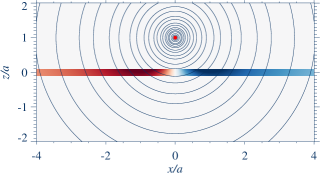
(a) The magnetic field: $\boldsymbol{B}$

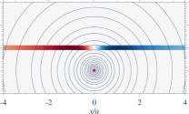
(b) The “potential” field: $\boldsymbol{P}$

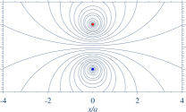
(c) The “closed” field: $\boldsymbol{B}_{\mathrm{cl}}$

Figure 1: The entangled physical origins of LABEL:sub@fig:B the magnetic field $\boldsymbol{B}=\boldsymbol{P}+\boldsymbol{B}_{\mathrm{cl}}$ for $z>0$ when it is decomposed into the fields LABEL:sub@fig:BP $\boldsymbol{P}$ which thread the boundary at $z=0$ and are potential for $z>0$ and LABEL:sub@fig:BC $\boldsymbol{B}_{\mathrm{cl}}$ which close on themselves for $z>0$. A red dot indicates a line current, $I\,\hat{\boldsymbol{y}}$, directed away from the observer and a blue dot indicates a line current, $-I\,\hat{\boldsymbol{y}}$, towards the observer. The black lines are contours of the vector potential that trace magnetic field lines. The color scale along $z=0$ corresponds to the vertical magnetic field component with red/blue corresponding to up/down. All three magnetic fields, $\boldsymbol{B}$, $\boldsymbol{P}$, and $\boldsymbol{B}_{\mathrm{cl}}$, are produced by a physical current $I\,\hat{\boldsymbol{y}}$ at $x/a=0;z/a=1$, but $\boldsymbol{P}$ is represented by an image current $I\,\hat{\boldsymbol{y}}$ at $x/a=0;z/a=-1$, while $\boldsymbol{B}_{\mathrm{cl}}$ is represented by a physical current $I\,\hat{\boldsymbol{y}}$ at $x/a=0;z/a=1$ and an image current $-I\,\hat{\boldsymbol{y}}$ at $x/a=0;z/a=-1$.

The gauge non-invariance of the magnetic helicity $H$ is closely related to the flux threading the bounding surface ${\partial\mathcal{V}}$. This flux is often mis-attributed to ‘exterior linkage’ similar to the way the potential field $\boldsymbol{P}$ is often confused with ‘external linkage’ (see pp 30-31 in Blackman, 2014). Consider the Cartesian $\left(\hat{\boldsymbol{x}},\hat{\boldsymbol{y}},\hat{\boldsymbol{z}}\right)$ geometry of Figure 1 where $\mathcal{V}=\left(x,y,z>0\right)$ corresponds to the domain of interest bounded by ${\partial\mathcal{V}}$ at $z=0$. Let this domain $\mathcal{V}$ contain a line current $I\,\hat{\boldsymbol{y}}$ at $x/a=0$ and $z/a=1$. Figure 1a shows the physical current source indicated by the red dot and contours of the vector potential tracing the magnetic field lines. The color scale represents $B_{z}$ at $z=0$ (the normal component at ${\partial\mathcal{V}}$) with red being positive and blue negative. All of the physical current sources in this example are contained inside the volume of interest $\mathcal{V}$! Using the generalized “method of images” Thomson (1845); Hammond (1960) any magnetic field $\boldsymbol{B}$ in $\mathcal{V}$ may be decomposed into two components $\boldsymbol{B}=\boldsymbol{P}+\boldsymbol{B}_{\mathrm{cl}}$: a magnetic field $\boldsymbol{P}$ that is potential in $\mathcal{V}$ and threads the boundary and a magnetic field $\boldsymbol{B}_{\mathrm{cl}}$ that closes on itself in $\mathcal{V}$, i.e., $\hat{\boldsymbol{n}}\cdot\boldsymbol{B}_{\mathrm{cl}}|_{\partial\mathcal{V}}=0$. For example, one can always find a mathematically unique potential field $\boldsymbol{P}$ in $\mathcal{V}$ corresponding to the normal component of $\boldsymbol{B}$ on the surface $z=0$, i.e., corresponding to the flux threading this bounding surface. This potential field, shown in Figure 1b, is represented by an image current $I\,\hat{\boldsymbol{y}}$ outside the volume of interest $\mathcal{V}$ at $x/a=0$ and $z/a=-1$ in ${\mathcal{V}^{*}}$, as $\boldsymbol{\nabla}\boldsymbol{\times}\boldsymbol{P}=0$ must be zero inside $\mathcal{V}$. Thus, the representation of flux threading the boundary by a potential field $\boldsymbol{P}$ misattributes the origin of this flux to a current source outside the volume of interest $\mathcal{V}$ Schuck et al. (2022). Similarly, the magnetic component that closes in $\mathcal{V}$, defined as $\boldsymbol{B}_{\mathrm{cl}}\equiv\boldsymbol{B}-\boldsymbol{P}$ and shown in Figure 1c, is represented by two anti-parallel currents: one corresponds to the physical current $I\,\hat{\boldsymbol{y}}$ in $\mathcal{V}$ and the other corresponds to its image current $-I\,\hat{\boldsymbol{y}}$. The image current is symmetrically placed across the boundary ${\partial\mathcal{V}}$ to ensure $\hat{\boldsymbol{n}}\cdot\boldsymbol{B}_{\mathrm{cl}}|_{\partial\mathcal{V}}=0$ at $z=0$ by construction. While mathematically $\boldsymbol{P}$ is an ‘external linkage,’ its physical origin is internal to $\mathcal{V}$! The superposition of $\boldsymbol{P}$ and $\boldsymbol{B}_{\mathrm{cl}}$ recovers the total magnetic field because the image currents in ${\mathcal{V}^{*}}$ cancel and all that remains is the physical current source inside $\mathcal{V}$. However, the decomposition for this example results in the apparent non-sequitur that the potential field $\boldsymbol{P}$ is curl free $\boldsymbol{\nabla}\boldsymbol{\times}\boldsymbol{P}=0$ in $\mathcal{V}$ but indeed physically produced by currents in $\mathcal{V}$! This example shows how easily the origins of magnetic fields can be confused by expressing them in forms that are mathematically convenient, for example, for calculating relative helicity. Yet the origins of these fields are of critical importance for understanding cause and effect, and so a means for tracking these origins while simultaneously calculating global quantities such as the relative helicity or magnetic energy is key for a complete understanding of dynamical astrophysical phenomena.

The primary purpose of this paper is to disentangle the linkages that originate with internal and external current sources in relative helicity for open systems. This work is organized as follows: §2 establishes the framework for attributing magnetic fields to electric current sources, §3 briefly discusses helicity in magnetically closed systems, §4 reviews the concepts of relative helicity for magnetically open systems, §5 extends relative helicity to simultaneously characterize the open-open and open-closed helicities as well as the domains of origin of the linked magnetic fields and develops novel expressions for internal and external relative helicity and internal-external relative helicity based on the domain of origin of the magnetic field in currents, §6 describes some of the implications of this work for the concept of free energy and §7 discusses the implications of these results for theory and observation.

2 The Attribution of Magnetic of Field to Internal and External Current Sources

The attribution of magnetic fields to physical current sources is necessary to fully understand cause and effect, the linkages of helicity, and changes in magnetic energy within a volume of interest $\mathcal{V}$. In classical electromagnetic theory, currents create magnetic fields. This statement is inherent in the Biot-Savart law Biot & Savart (1820) written in continuous form

$$\boldsymbol{B}\left(t,\boldsymbol{x}\right)=\frac{1}{c}\,\boldsymbol{\nabla}\boldsymbol{\times}\int\limits_{{\mathbb{R}^{3}}}{d^{3}x^{\prime}}\,\frac{\boldsymbol{J}\left(t,\boldsymbol{x}^{\prime}\right)}{\left|\boldsymbol{x}-\boldsymbol{x}^{\prime}\right|}=\frac{1}{c}\,\int\limits_{{\mathbb{R}^{3}}}{d^{3}x^{\prime}}\,\boldsymbol{J}\left(t,\boldsymbol{x}^{\prime}\right)\boldsymbol{\times}\frac{\boldsymbol{x}-\boldsymbol{x}^{\prime}}{\left|\boldsymbol{x}-\boldsymbol{x}^{\prime}\right|^{3}}\qquad\boldsymbol{x}\in{\mathbb{R}^{3}},$$ (3)

as a convolution with spatial moments of the free space Green’s function, where $c$ is the speed of light. In the right-most expression there are no spatial or temporal derivatives operating on the source $\boldsymbol{J}$. Green’s functions form the basis for understanding cause and effect in physics. Loosely speaking, the Green’s function propagates a “cause” at $\boldsymbol{x}^{\prime}$ to an “effect” at $\boldsymbol{x}$. This is how nature works despite the practice in MHD analysis to substitute $\boldsymbol{J}\Longrightarrow{c}\,\boldsymbol{\nabla}\boldsymbol{\times}\boldsymbol{B}/\left(4\,\pi\right)$ into the $\boldsymbol{J}\boldsymbol{\times}\boldsymbol{B}$ force to eliminate any explicit reference to $\boldsymbol{J}$ in MHD. Physically, the current $\boldsymbol{J}$ is manifestly the source of the magnetic vorticity. The Biot-Savart law provides attribution of a current element at $\boldsymbol{x}^{\prime}$ to the magnetic field at the location $\boldsymbol{x}$. In the pre-Maxwell formulation of electrodynamics, the magnetic field $\boldsymbol{B}$ at $\boldsymbol{x}$ depends on currents at all other points in the universe ${\mathbb{R}^{3}}$. Realistically, this universe dynamically corresponds to $\mathbb{R}\ll{c}\,\Delta t$. This has deep implications—the magnetic field is a non-local field despite the fact that it is often conceptually treated as a local object in MHD. Changes in $\boldsymbol{B}\left(t,\boldsymbol{x}\right)$ imply changes in $\boldsymbol{J}\left(t,\boldsymbol{x}^{\prime}\right)$ somewhere else!

While Equation (3) is intuitive, it is nearly impossible to apply in practice because access to complete information about all currents in the entire universe $\boldsymbol{x}\in{\mathbb{R}^{3}}$ is rare. Rather, in most cases, knowledge is limited to currents and magnetic fields in a volume $\mathcal{V}$ bounded by a surface ${\partial\mathcal{V}}$. Consider a simply connected internal volume $\mathcal{V}$ bounded by closed surface ${\partial\mathcal{V}}$ and an external domain denoted ${\mathcal{V}^{*}}$ such that ${\mathbb{R}^{3}}=\mathcal{V}+{\mathcal{V}^{*}}$. Suppose that both domains contain corresponding current systems $\boldsymbol{J}$ and $\boldsymbol{J}^{*}$. By the electromagnetic superposition principle, the total magnetic field in Equation (3) is then

$$\boldsymbol{B}\left(t,\boldsymbol{x}\right)=\boldsymbol{B}_{\mathrm{BS}}\left(\boldsymbol{J};t,\boldsymbol{x}\right)+\boldsymbol{B}_{\mathrm{BS}}\left(\boldsymbol{J}^{*};t,\boldsymbol{x}\right)\qquad\boldsymbol{x}\in{\mathbb{R}^{3}},$$ (4a)

with

$$\boldsymbol{B}_{\mathrm{BS}}\left(\boldsymbol{J};t,\boldsymbol{x}\right)=\overbrace{\frac{1}{c}\,\boldsymbol{\nabla}\boldsymbol{\times}\int\limits_{\mathcal{V}}{d^{3}x^{\prime}}\,\frac{\boldsymbol{J}\left(t,\boldsymbol{x}^{\prime}\right)}{\left|\boldsymbol{x}-\boldsymbol{x}^{\prime}\right|}}^{\mbox{Internal Sources}}\qquad\boldsymbol{x}\in{\mathbb{R}^{3}},$$ (4b)

$$\boldsymbol{B}_{\mathrm{BS}}\left(\boldsymbol{J}^{*};t,\boldsymbol{x}\right)=\overbrace{\frac{1}{c}\,\boldsymbol{\nabla}\boldsymbol{\times}\int\limits_{{\mathcal{V}^{*}}}{d^{3}x^{\prime}}\,\frac{\boldsymbol{J}^{*}\left(t,\boldsymbol{x}^{\prime}\right)}{\left|\boldsymbol{x}-\boldsymbol{x}^{\prime}\right|}}^{\mbox{External Sources}}\qquad\boldsymbol{x}\in{\mathbb{R}^{3}},$$ (4c)

where the total field is comprised of two integrants: one produced by internal sources, $\boldsymbol{J}$ in $\mathcal{V}$, and one produced by external sources, $\boldsymbol{J}^{*}$ in ${\mathcal{V}^{*}}$. Both integrants (4b) and (4c) are continuous vector fields for $\boldsymbol{x}\in{\mathbb{R}^{3}}$. If $\boldsymbol{J}$ and $\boldsymbol{B}$ are completely known in $\mathcal{V}$ then $\boldsymbol{B}_{\mathrm{BS}}\left(\boldsymbol{J};t,\boldsymbol{x}\right)$ can be computed directly by convolution and $\boldsymbol{B}_{\mathrm{BS}}\left(\boldsymbol{J}^{*};t,\boldsymbol{x}\right)$ in $\mathcal{V}$ may be computed from Equation (4a). Analogously, if $\boldsymbol{B}$ in $\mathcal{V}$ is known and $\boldsymbol{B}_{\mathrm{BS}}\left(\boldsymbol{J}^{*};t,\boldsymbol{x}\right)$ can be estimated then $\boldsymbol{B}_{\mathrm{BS}}\left(\boldsymbol{J};t,\boldsymbol{x}\right)$ in $\mathcal{V}$ may be computed from Equation (4a). Below we show that $\boldsymbol{B}_{\mathrm{BS}}\left(\boldsymbol{J};t,\boldsymbol{x}\right)$ and $\boldsymbol{B}_{\mathrm{BS}}\left(\boldsymbol{J}^{*};t,\boldsymbol{x}\right)$ in $\mathcal{V}$ and $\boldsymbol{B}_{\mathrm{BS}}\left(\boldsymbol{J};t,\boldsymbol{x}\right)$ in ${\mathcal{V}^{*}}$ may be computed from $\boldsymbol{B}$ in $\mathcal{V}\cup{\partial\mathcal{V}}$ without performing computationally expensive Biot-Savart convolution integrals by leveraging the powerful fundamental theorem of vector calculus. For the remainder of the paper we include the source $\boldsymbol{J}$ or $\boldsymbol{J}^{*}$ as an argument to the vector field when the source of the magnetic field is of interest. For example, $\boldsymbol{P}\left(\boldsymbol{J};t,\boldsymbol{x}\right)$ and $\boldsymbol{B}_{\mathrm{cl}}\left(\boldsymbol{J};t,\boldsymbol{x}\right)$ are, respectively, the potential magnetic field and the magnetic field that closes in $\mathcal{V}$ determined from the magnetic field $\boldsymbol{B}_{\mathrm{BS}}\left(\boldsymbol{J};t,\boldsymbol{x}\right)$ produced by currents $\boldsymbol{J}$ in $\mathcal{V}$. Correspondingly $\boldsymbol{P}\left(\boldsymbol{J}^{*};t,\boldsymbol{x}\right)$ and $\boldsymbol{B}_{\mathrm{cl}}\left(\boldsymbol{J}^{*};t,\boldsymbol{x}\right)$ are, respectively, the potential magnetic field and the magnetic field that closes in $\mathcal{V}$ determined from the magnetic field $\boldsymbol{B}_{\mathrm{BS}}\left(\boldsymbol{J}^{*};t,\boldsymbol{x}\right)$ produced by currents $\boldsymbol{J}^{*}$ in ${\mathcal{V}^{*}}$. And finally, $\boldsymbol{B}\left(t,\boldsymbol{x}\right)$ without the argument of current represents the total magnetic field at $t$ and $\boldsymbol{x}$ in Equation (4a).

2.1 The Fundamental Theorem of Vector Calculus: The Helmholtz Decomposition

Consider the fundamental theorem of vector calculus (the Helmholtz Decomposition, HD) for a vector field $\boldsymbol{F}\left(\boldsymbol{x}\right)$ in $\mathcal{V}$ Morse & Feshbach (1953); Gui & Dou (2007); Kustepeli (2016)

$$\boldsymbol{\mathcal{F}}_{\mathrm{HD}}\left(\boldsymbol{x}\right)=\boldsymbol{\nabla}\boldsymbol{\times}\boldsymbol{A}\left(\boldsymbol{x}\right)-\boldsymbol{\nabla}\Psi\left(\boldsymbol{x}\right),$$ (5a)

where

$$\boldsymbol{A}\left(\boldsymbol{x}\right)= \frac{1}{4\,\pi}\,\left[\int\limits_{\mathcal{V}}{\!d^{3}x^{\prime}}\frac{\boldsymbol{\nabla}^{\prime}\boldsymbol{\times}\boldsymbol{F}\left(\boldsymbol{x}^{\prime}\right)}{\left|\boldsymbol{x}-\boldsymbol{x}^{\prime}\right|}+\oint\limits_{\partial\mathcal{V}}{dS^{\prime}}\,\frac{\hat{\boldsymbol{n}}^{\prime}\boldsymbol{\times}\boldsymbol{F}\left(\boldsymbol{x}^{\prime}\right)}{\left|\boldsymbol{x}-\boldsymbol{x}^{\prime}\right|}\right],$$ (5b)

$$\Psi\left(\boldsymbol{x}\right)= \frac{1}{4\,\pi}\,\left[\int\limits_{\mathcal{V}}{\!d^{3}x^{\prime}}\frac{\boldsymbol{\nabla}^{\prime}\cdot\boldsymbol{F}\left(\boldsymbol{x}^{\prime}\right)}{\left|\boldsymbol{x}-\boldsymbol{x}^{\prime}\right|}+\oint\limits_{\partial\mathcal{V}}{dS^{\prime}}\,\frac{\hat{\boldsymbol{n}}^{\prime}\cdot\boldsymbol{F}\left(\boldsymbol{x}^{\prime}\right)}{\left|\boldsymbol{x}-\boldsymbol{x}^{\prime}\right|}\right],$$ (5c)

where $$\hat{\boldsymbol{n}} \mathcal{V} \boldsymbol{x} \mathcal{V} {\mathcal{V}^{*}} {\partial\mathcal{V}}$$ points into . There is a jump discontinuity in the value of the surface integrals as the observation point passes from to across a smooth surface producing

$$\boldsymbol{\mathcal{F}}_{\mathrm{HD}}\left(\boldsymbol{x}\right)=\left\{\begin{array}[]{ll}\boldsymbol{F}\left(\boldsymbol{x}\right)&\boldsymbol{x}\in\mathcal{V},\\ \boldsymbol{F}\left(\boldsymbol{x}\right)/2&\boldsymbol{x}\in{\partial\mathcal{V}},\\ 0&\boldsymbol{x}\in{\mathcal{V}^{*}}.\end{array}\right.$$ (5d)

The HD is a mathematical reconstruction theorem. It is ignorant of electromagnetic theory and does not inherently preserve physical properties of the field $\boldsymbol{F}\left(\boldsymbol{x}\right)$ across the boundary ${\partial\mathcal{V}}$. For example, if $\boldsymbol{F}$ is solenoidal for $\boldsymbol{x}\in{\mathbb{R}^{3}}$, then generally Equation (5d) will not maintain this property, e.g., continuity of $\hat{\boldsymbol{n}}\cdot\boldsymbol{F}$, across ${\partial\mathcal{V}}$. Furthermore, its value on a smooth surface converges to half the value just inside the boundary, which is an inconvenient property for astrophysical problems that involve physics in notional surfaces between domains, such as a photosphere. This motivates the alternative definition (see for example Kempka et al., 1996)

$$\alpha\left(\boldsymbol{x}\right)\boldsymbol{\mathfrak{F}}_{\mathrm{HD}}\left(\boldsymbol{x}\right)=\boldsymbol{\nabla}\boldsymbol{\times}\boldsymbol{A}\left(\boldsymbol{x}\right)-\boldsymbol{\nabla}\Psi\left(\boldsymbol{x}\right),$$ (6a)

$$\alpha\left(\boldsymbol{x}\right)=\frac{\chi\left(\boldsymbol{x}\right)}{4\,\pi}=\left\{\begin{array}[]{ll}1&\boldsymbol{x}\in\mathcal{V}\\ \left.\begin{array}[]{ll}1/2&\mbox{smooth surfaces}\\ 1/4&\mbox{edges of $\mathcal{V}$}\\ 1/8&\mbox{vertices of $\mathcal{V}$}\end{array}\right\}&\boldsymbol{x}\in{\partial\mathcal{V}}\\ 0&\boldsymbol{x}\in{\mathcal{V}^{*}}\end{array}\right.,$$ (6b)

where $$\chi\left(\boldsymbol{x}\right) {\partial\mathcal{V}} \alpha\left(\boldsymbol{x}\right) \boldsymbol{x}\in\mathcal{V} \boldsymbol{x}\in{\mathcal{V}^{*}} \boldsymbol{x}\in{\partial\mathcal{V}} \alpha\left(\boldsymbol{x}\right) \boldsymbol{x} {\partial\mathcal{V}} \boldsymbol{x}\in\mathcal{V} \boldsymbol{x}\in{\mathcal{V}^{*}} {\partial\mathcal{V}} \alpha=1/2 \mathcal{V} {\mathcal{V}^{*}} \alpha=1/2 \alpha=1/4 \alpha=1/8 \alpha=1 \boldsymbol{x}\in\mathcal{V} \alpha=0 \boldsymbol{x}\in{\mathcal{V}^{*}} \mathcal{V}$$ is the local internal solid angle of the principal volume at the observation point on Kellogg (1929); Courant & Hilbert (1989a, b); Bladel (1991). The factor is a constant, and therefore continuous and differentiable, on the open sets and which do not contain . The factor takes on other values when lies in the boundary because the principle volume of the observation point projects into both domains and . On smooth boundaries with well-defined tangent surfaces , i.e., half the principle volume lies in and half in . By analogy, for a cube, which is smooth almost everywhere, on faces, on edges, and at vertices (of a cuboid) and of course for and for , consistent with the projections of the fractions of the principal volumes into .

The $\alpha\left(\boldsymbol{x}\right)$ on the left of Equation (6a) ensures that the surface values of $\boldsymbol{\mathfrak{F}}_{\mathrm{HD}}\left(\boldsymbol{x}\right)$ are continuous from within the volume $\mathcal{V}$ as defined by the one-sided limiting process

$$\lim_{\boldsymbol{x}\in\mathcal{V}\rightarrow\boldsymbol{x}\in{\partial\mathcal{V}}}\boldsymbol{\mathfrak{F}}_{\mathrm{HD}}\left(\boldsymbol{x}\right)=\boldsymbol{F}\left(\boldsymbol{x}\right).$$ (6c)

Consequently

$$\boldsymbol{\mathfrak{F}}_{\mathrm{HD}}\left(\boldsymbol{x}\right)=\left\{\begin{array}[]{ll}\boldsymbol{F}\left(\boldsymbol{x}\right)&\boldsymbol{x}\in\mathcal{V}\cup{\partial\mathcal{V}},\\ \mbox{Arbitrary}&\boldsymbol{x}\in{\mathcal{V}^{*}}.\end{array}\right.$$ (6d)

$\boldsymbol{\mathfrak{F}}_{\mathrm{HD}}\left(\boldsymbol{x}\right)$ is arbitrary in ${\mathcal{V}^{*}}$ because $\alpha\left(\boldsymbol{x}\right)=0$ on the left-hand side of Equation (6a) for $\boldsymbol{x}\in{\mathcal{V}^{*}}$. Thus, $\boldsymbol{\mathfrak{F}}_{\mathrm{HD}}\left(\boldsymbol{x}\right)$ can formally be defined in ${\mathcal{V}^{*}}$ to properly preserve physical properties of $\boldsymbol{F}\left(\boldsymbol{x}\right)$ across ${\partial\mathcal{V}}$.

For a solenoidal field, the divergence term in (5c) may be ignored and expression $\boldsymbol{\mathfrak{F}}_{\mathrm{HD}}\left(\boldsymbol{x}\right)$ for the magnetic field becomes

$$\alpha\left(\boldsymbol{x}\right)\,\boldsymbol{B}_{\mathrm{HD}}\left(t,\boldsymbol{x}\right)=\frac{1}{4\,\pi}\,\boldsymbol{\nabla}\boldsymbol{\times}\int\limits_{\mathcal{V}}{d^{3}x^{\prime}}\frac{\boldsymbol{\nabla}^{\prime}\boldsymbol{\times}\boldsymbol{B}\left(t,\boldsymbol{x}^{\prime}\right)}{\left|\boldsymbol{x}-\boldsymbol{x}^{\prime}\right|}+\frac{1}{4\,\pi}\,\left[\boldsymbol{\nabla}\boldsymbol{\times}\oint\limits_{\partial\mathcal{V}}{dS^{\prime}}\,\frac{\hat{\boldsymbol{n}}^{\prime}\boldsymbol{\times}\boldsymbol{B}\left(t,\boldsymbol{x}^{\prime}\right)}{\left|\boldsymbol{x}-\boldsymbol{x}^{\prime}\right|}-\boldsymbol{\nabla}\oint\limits_{\partial\mathcal{V}}{dS^{\prime}}\,\frac{\hat{\boldsymbol{n}}^{\prime}\cdot\boldsymbol{B}\left(t,\boldsymbol{x}^{\prime}\right)}{\left|\boldsymbol{x}-\boldsymbol{x}^{\prime}\right|}\right]\qquad\boldsymbol{x}\in{\mathbb{R}^{3}}.$$ (7)

As mentioned above, this does not constrain $\boldsymbol{B}_{\mathrm{HD}}$ in the external universe where $\alpha\left(\boldsymbol{x}\right)=0$. Strictly speaking, if there is flux threading the boundary ${\partial\mathcal{V}}$ then the magnetic field determined by Equation (7) for $\boldsymbol{x}\in\mathcal{V}\cup{\partial\mathcal{V}}$ should be formally matched to a potential field in the external universe $\boldsymbol{x}\in{\mathcal{V}^{*}}$ to preserve the solenoidal property of $\boldsymbol{B}$ across ${\partial\mathcal{V}}$, i.e., as discussed in relation to Equation (6d) above for $\boldsymbol{x}\in{\mathcal{V}^{*}}$. However, practically speaking, this matching procedure is usually unnecessary as we are often interested in reconstructing 1. $\boldsymbol{B}$for $\boldsymbol{x}\in\mathcal{V}\cup{\partial\mathcal{V}}$ or determining 2. $\boldsymbol{B}_{\mathrm{BS}}\left(\boldsymbol{J}^{*};t,\boldsymbol{x}\right)$for $\boldsymbol{x}\in\mathcal{V}\cup{\partial\mathcal{V}}$ or 3. $\boldsymbol{B}_{\mathrm{BS}}\left(\boldsymbol{J};t,\boldsymbol{x}\right)$for $\boldsymbol{x}\in{\mathbb{R}^{3}}$ as discussed below.

2.2 Linking Magnetic Fields to their Current Sources

If the net displacement current is ignorable, then Ampère’s law

$$\boldsymbol{\nabla}\boldsymbol{\times}\boldsymbol{B}=\frac{4\,\pi}{c}\,\boldsymbol{J},$$ (8)

may be substituted into the volume integral to produce

$$\alpha\left(\boldsymbol{x}\right)\,\boldsymbol{B}_{\mathrm{HD}}\left(t,\boldsymbol{x}\right)=\frac{1}{c}\,\boldsymbol{\nabla}\boldsymbol{\times}\int\limits_{\mathcal{V}}{d^{3}x^{\prime}}\frac{\boldsymbol{J}\left(t,\boldsymbol{x}^{\prime}\right)}{\left|\boldsymbol{x}-\boldsymbol{x}^{\prime}\right|}+\frac{1}{4\,\pi}\,\left[\boldsymbol{\nabla}\boldsymbol{\times}\oint\limits_{\partial\mathcal{V}}{dS^{\prime}}\,\frac{\hat{\boldsymbol{n}}^{\prime}\boldsymbol{\times}\boldsymbol{B}\left(t,\boldsymbol{x}^{\prime}\right)}{\left|\boldsymbol{x}-\boldsymbol{x}^{\prime}\right|}-\boldsymbol{\nabla}\oint\limits_{\partial\mathcal{V}}{dS^{\prime}}\,\frac{\hat{\boldsymbol{n}}^{\prime}\cdot\boldsymbol{B}\left(t,\boldsymbol{x}^{\prime}\right)}{\left|\boldsymbol{x}-\boldsymbol{x}^{\prime}\right|}\right]\qquad\boldsymbol{x}\in{\mathbb{R}^{3}}.$$ (9)

Equation (4a) unambiguously associates the Biot-Savart integrals over current systems $\boldsymbol{J}$ and $\boldsymbol{J}^{*}$ to their corresponding magnetic field components $\boldsymbol{B}_{\mathrm{BS}}\left(\boldsymbol{J};t,\boldsymbol{x}\right)$ and $\boldsymbol{B}_{\mathrm{BS}}\left(\boldsymbol{J}^{*};t,\boldsymbol{x}\right)$, establishing cause and effect. This pre-Maxwell equation also implies that the magnetic field $\boldsymbol{B}\left(t,\boldsymbol{x}\right)$ at any location contains entangled magnetic contributions from both internal $\boldsymbol{J}$ and external $\boldsymbol{J}^{*}$ current systems. Thus, the surface integrals in Equation (9) implicitly also contain entangled magnetic contributions from both internal $\boldsymbol{J}$ and external $\boldsymbol{J}^{*}$ current systems. As shown below, these contributions separate cleanly when $\boldsymbol{x}\in\mathcal{V}$ or $\boldsymbol{x}\in{\mathcal{V}^{*}}$ but are entangled when the observation point is in the boundary $\boldsymbol{x}\in{\partial\mathcal{V}}$.

Since the factor $\alpha\left(\boldsymbol{x}\right)$ is chosen to enforce continuity of the HD from $\mathcal{V}$ to ${\partial\mathcal{V}}$, as in Equation (6c), the discussion of (9) is divided logically into two domains $\boldsymbol{x}\in\mathcal{V}\cup{\partial\mathcal{V}}$ and $\boldsymbol{x}\in{\mathcal{V}^{*}}$. For $\boldsymbol{x}\in\mathcal{V}\cup{\partial\mathcal{V}}$, Equation (9) becomes

$$\boldsymbol{B}\left(t,\boldsymbol{x}\right)=\frac{1}{\alpha\left(\boldsymbol{x}\right)\,c}\,\boldsymbol{\nabla}\boldsymbol{\times}\int\limits_{\mathcal{V}}{d^{3}x^{\prime}}\frac{\boldsymbol{J}\left(t,\boldsymbol{x}^{\prime}\right)}{\left|\boldsymbol{x}-\boldsymbol{x}^{\prime}\right|}+\frac{1}{4\,\pi\,\alpha\left(\boldsymbol{x}\right)}\,\left[\boldsymbol{\nabla}\boldsymbol{\times}\oint\limits_{\partial\mathcal{V}}{dS^{\prime}}\,\frac{\hat{\boldsymbol{n}}^{\prime}\boldsymbol{\times}\boldsymbol{B}\left(t,\boldsymbol{x}^{\prime}\right)}{\left|\boldsymbol{x}-\boldsymbol{x}^{\prime}\right|}-\boldsymbol{\nabla}\oint\limits_{\partial\mathcal{V}}{dS^{\prime}}\,\frac{\hat{\boldsymbol{n}}^{\prime}\cdot\boldsymbol{B}\left(t,\boldsymbol{x}^{\prime}\right)}{\left|\boldsymbol{x}-\boldsymbol{x}^{\prime}\right|}\right]\qquad\boldsymbol{x}\in\mathcal{V}\cup{\partial\mathcal{V}},$$ (10)

which addresses the reconstruction in item 1 above. Equations (4a) and (10) are equivalent in the intersection of their domain of validity $x\in\mathcal{V}\cup{\partial\mathcal{V}}$. This equivalence will be used to establish the formal correspondence between $\boldsymbol{B}_{\mathrm{BS}}\left(\boldsymbol{J};t,\boldsymbol{x}\right)$ and $\boldsymbol{B}_{\mathrm{BS}}\left(\boldsymbol{J}^{*};t,\boldsymbol{x}\right)$ in Equations (4b)-(4c) and the HD in Equation (10).

To establish the correspondence between internal and external sources in Equation (4a) and terms in (10), the Biot-Savart magnetic field produced by internal sources in the volume $\mathcal{V}$ from Equation (4b) is added to and subtracted from Equation (10) to produce for $\boldsymbol{x}\in\mathcal{V}\cup{\partial\mathcal{V}}$

$$\boldsymbol{B}\left(t,\boldsymbol{x}\right)= \underbrace{\overbrace{\frac{1}{c}\,\boldsymbol{\nabla}\boldsymbol{\times}\int\limits_{\mathcal{V}}{\!d^{3}x^{\prime}}\frac{\boldsymbol{J}\left(t,\boldsymbol{x}^{\prime}\right)}{\left|\boldsymbol{x}-\boldsymbol{x}^{\prime}\right|}}^{\mbox{Internal Sources}}}_{\boldsymbol{B}_{\mathrm{BS}}\left(\boldsymbol{J};t,\boldsymbol{x}\right)}$$ (11)

$$\qquad+\underbrace{\overbrace{\frac{1-\alpha\left(\boldsymbol{x}\right)}{\alpha\left(\boldsymbol{x}\right)\,c}\,\boldsymbol{\nabla}\boldsymbol{\times}\int\limits_{\mathcal{V}}{\!d^{3}x^{\prime}}\frac{\boldsymbol{J}\left(t,\boldsymbol{x}^{\prime}\right)}{\left|\boldsymbol{x}-\boldsymbol{x}^{\prime}\right|}+\frac{1}{4\,\pi\,\alpha\left(\boldsymbol{x}\right)}\,\left[\boldsymbol{\nabla}\boldsymbol{\times}\oint\limits_{\partial\mathcal{V}}{dS^{\prime}}\,\frac{\hat{\boldsymbol{n}}^{\prime}\boldsymbol{\times}\boldsymbol{B}\left(t,\boldsymbol{x}^{\prime}\right)}{\left|\boldsymbol{x}-\boldsymbol{x}^{\prime}\right|}-\boldsymbol{\nabla}\oint\limits_{\partial\mathcal{V}}{dS^{\prime}}\,\frac{\hat{\boldsymbol{n}}^{\prime}\cdot\boldsymbol{B}\left(t,\boldsymbol{x}^{\prime}\right)}{\left|\boldsymbol{x}-\boldsymbol{x}^{\prime}\right|}\right]}^{\mbox{External Sources}}}_{\boldsymbol{B}_{\mathrm{BS}}\left(\boldsymbol{J}^{*};t,\boldsymbol{x}\right)},$$

where the terms are now grouped according to their physical interpretation. This resolves items 2 and 3 for $\boldsymbol{x}\in\mathcal{V}\cup{\partial\mathcal{V}}$. However, as discussed below, there are more efficient computational expressions for $\boldsymbol{B}_{\mathrm{BS}}\left(\boldsymbol{J};t,\boldsymbol{x}\right)$ and $\boldsymbol{B}_{\mathrm{BS}}\left(\boldsymbol{J}^{*};t,\boldsymbol{x}\right)$ when the bounding surface is excluded, i.e., $\boldsymbol{x}\in\mathcal{V}$ or $\boldsymbol{x}\in{\mathcal{V}^{*}}$. Note that the formal appearance of the integrant due to internal sources proportional to $\boldsymbol{B}_{\mathrm{BS}}\left(\boldsymbol{J};t,\boldsymbol{x}\right)$ under “External Sources” in Equation (11) is a consequence of the entanglement of internal and external sources of $\boldsymbol{B}$ in evaluation of the surface integrals when the observation point is in the boundary $\boldsymbol{x}\in{\partial\mathcal{V}}$. The surface integrals depend on total magnetic field $\boldsymbol{B}\left(t,x\right)$ which implicitly contains entangled magnetic contributions from internal and external current sources. If we exclude the observation points in the surface, then $\alpha\left(\boldsymbol{x}\right)=1$ and, for observation points in the volume of interest, Equation (11) reduces to the intuitive form

$$\boldsymbol{B}\left(t,\boldsymbol{x}\right)=\underbrace{\overbrace{\frac{1}{c}\,\boldsymbol{\nabla}\boldsymbol{\times}\int\limits_{\mathcal{V}}{\!d^{3}x^{\prime}}\frac{\boldsymbol{J}\left(t,\boldsymbol{x}^{\prime}\right)}{\left|\boldsymbol{x}-\boldsymbol{x}^{\prime}\right|}}^{\mbox{Internal Sources}}}_{\boldsymbol{B}_{\mathrm{BS}}\left(\boldsymbol{J};t,\boldsymbol{x}\right)}+\underbrace{\overbrace{\frac{1}{4\,\pi}\,\left[\boldsymbol{\nabla}\boldsymbol{\times}\oint\limits_{\partial\mathcal{V}}{dS^{\prime}}\,\frac{\hat{\boldsymbol{n}}^{\prime}\boldsymbol{\times}\boldsymbol{B}\left(t,\boldsymbol{x}^{\prime}\right)}{\left|\boldsymbol{x}-\boldsymbol{x}^{\prime}\right|}-\boldsymbol{\nabla}\oint\limits_{\partial\mathcal{V}}{dS^{\prime}}\,\frac{\hat{\boldsymbol{n}}^{\prime}\cdot\boldsymbol{B}\left(t,\boldsymbol{x}^{\prime}\right)}{\left|\boldsymbol{x}-\boldsymbol{x}^{\prime}\right|}\right]}^{\mbox{External Sources}}}_{\boldsymbol{B}_{\mathrm{BS}}\left(\boldsymbol{J}^{*};t,\boldsymbol{x}\right)}\qquad\boldsymbol{x}\in\mathcal{V}.$$ (12)

The surface integrals now provide an efficient expression for the magnetic field in $\mathcal{V}$ produced by external sources

$$\boldsymbol{B}_{\mathrm{BS}}\left(\boldsymbol{J}^{*};t,\boldsymbol{x}\right)= \boldsymbol{B}\left(t,\boldsymbol{x}\right)-\boldsymbol{B}_{\mathrm{BS}}\left(\boldsymbol{J};t,\boldsymbol{x}\right),$$ (13a)

$$= \frac{1}{4\,\pi}\,\left[\boldsymbol{\nabla}\boldsymbol{\times}\oint\limits_{\partial\mathcal{V}}{dS^{\prime}}\,\frac{\hat{\boldsymbol{n}}^{\prime}\boldsymbol{\times}\boldsymbol{B}\left(t,\boldsymbol{x}^{\prime}\right)}{\left|\boldsymbol{x}-\boldsymbol{x}^{\prime}\right|}-\boldsymbol{\nabla}\oint\limits_{\partial\mathcal{V}}{dS^{\prime}}\,\frac{\hat{\boldsymbol{n}}^{\prime}\cdot\boldsymbol{B}\left(t,\boldsymbol{x}^{\prime}\right)}{\left|\boldsymbol{x}-\boldsymbol{x}^{\prime}\right|}\right]=\overbrace{\frac{1}{c}\,\boldsymbol{\nabla}\boldsymbol{\times}\int\limits_{{\mathcal{V}^{*}}}{d^{3}x^{\prime}}\frac{\boldsymbol{J}^{*}\left(t,\boldsymbol{x}^{\prime}\right)}{\left|\boldsymbol{x}-\boldsymbol{x}^{\prime}\right|}}^{\mbox{External Sources}}\qquad\boldsymbol{x}\in\mathcal{V}.$$ (13b)

This establishes $$\boldsymbol{B}_{\mathrm{BS}}\left(\boldsymbol{J}^{*};t,\boldsymbol{x}\right) \boldsymbol{x}\in\mathcal{V} \boldsymbol{B}$$ for by surface convolution alone. This expression may be subtracted from the total field to provide an expression for the internal sources by surface convolution that is equivalent to the Biot-Savart law for internal sources

$$\boldsymbol{B}_{\mathrm{BS}}\left(\boldsymbol{J};t,\boldsymbol{x}\right)=\boldsymbol{B}\left(t,\boldsymbol{x}\right)-\boldsymbol{B}_{\mathrm{BS}}\left(\boldsymbol{J}^{*};t,\boldsymbol{x}\right)=\overbrace{\frac{1}{c}\,\boldsymbol{\nabla}\boldsymbol{\times}\int\limits_{\mathcal{V}}{d^{3}x^{\prime}}\frac{\boldsymbol{J}\left(t,\boldsymbol{x}^{\prime}\right)}{\left|\boldsymbol{x}-\boldsymbol{x}^{\prime}\right|}}^{\mbox{Internal Sources}}\qquad\boldsymbol{x}\in\mathcal{V}.$$ (13c)

Analogously, if we consider observation points in the external universe then $\alpha\left(\boldsymbol{x}\right)=0$ and the surface terms extinguish the internal terms as Equation (9) becomes

$$0=\underbrace{\overbrace{\frac{1}{c}\boldsymbol{\nabla}\boldsymbol{\times}\int\limits_{\mathcal{V}}{d^{3}x^{\prime}}\frac{\boldsymbol{J}\left(t,\boldsymbol{x}^{\prime}\right)}{\left|\boldsymbol{x}-\boldsymbol{x}^{\prime}\right|}}^{\mbox{Internal Sources}}}_{\boldsymbol{B}_{\mathrm{BS}}\left(\boldsymbol{J};t,\boldsymbol{x}\right)}+\underbrace{\overbrace{\frac{1}{4\,\pi}\,\left[\boldsymbol{\nabla}\boldsymbol{\times}\oint\limits_{\partial\mathcal{V}}{dS^{\prime}}\,\frac{\hat{\boldsymbol{n}}^{\prime}\boldsymbol{\times}\boldsymbol{B}\left(t,\boldsymbol{x}^{\prime}\right)}{\left|\boldsymbol{x}-\boldsymbol{x}^{\prime}\right|}-\boldsymbol{\nabla}\oint\limits_{\partial\mathcal{V}}{dS^{\prime}}\,\frac{\hat{\boldsymbol{n}}^{\prime}\cdot\boldsymbol{B}\left(t,\boldsymbol{x}^{\prime}\right)}{\left|\boldsymbol{x}-\boldsymbol{x}^{\prime}\right|}\right]}^{-\left(\mbox{Internal Sources}\right)}}_{-\boldsymbol{B}_{\mathrm{BS}}\left(\boldsymbol{J};t,\boldsymbol{x}\right)}\,\qquad\boldsymbol{x}\in{\mathcal{V}^{*}},$$ (14a)

where

$$\boldsymbol{B}_{\mathrm{BS}}\left(\boldsymbol{J};t,\boldsymbol{x}\right)=-\frac{1}{4\,\pi}\,\left[\boldsymbol{\nabla}\boldsymbol{\times}\oint\limits_{\partial\mathcal{V}}{dS^{\prime}}\,\frac{\hat{\boldsymbol{n}}^{\prime}\boldsymbol{\times}\boldsymbol{B}\left(t,\boldsymbol{x}^{\prime}\right)}{\left|\boldsymbol{x}-\boldsymbol{x}^{\prime}\right|}-\boldsymbol{\nabla}\oint\limits_{\partial\mathcal{V}}{dS^{\prime}}\,\frac{\hat{\boldsymbol{n}}^{\prime}\cdot\boldsymbol{B}\left(t,\boldsymbol{x}^{\prime}\right)}{\left|\boldsymbol{x}-\boldsymbol{x}^{\prime}\right|}\right]=\overbrace{\frac{1}{c}\,\boldsymbol{\nabla}\boldsymbol{\times}\int\limits_{\mathcal{V}}{d^{3}x^{\prime}}\frac{\boldsymbol{J}\left(t,\boldsymbol{x}^{\prime}\right)}{\left|\boldsymbol{x}-\boldsymbol{x}^{\prime}\right|}}^{\mbox{Internal Sources}}\qquad\boldsymbol{x}\in{\mathcal{V}^{*}}.$$ (14b)

Equations (13b) and (14b) manifestly show that the surface integrals contain contributions to the magnetic field from both internal and external currents and that these contributions separate out cleanly for observation points $\boldsymbol{x}\in\mathcal{V}$ or $\boldsymbol{x}\in{\mathcal{V}^{*}}$ but are entangled for $\boldsymbol{x}\in{\partial\mathcal{V}}$. Equations (13b)-(13c) and (14b) establish $\boldsymbol{B}_{\mathrm{BS}}\left(\boldsymbol{J};t,\boldsymbol{x}\right)$ for $\boldsymbol{x}\in\mathcal{V}$ in item 3 by surface convolution alone. Note that even if $\boldsymbol{B}_{\mathrm{BS}}\left(\boldsymbol{J};t,\boldsymbol{x}\right)$ or $\boldsymbol{B}_{\mathrm{BS}}\left(\boldsymbol{J}^{*};t,\boldsymbol{x}\right)$ are required on ${\partial\mathcal{V}}$, this computation necessitates the evaluation of the Biot-Savart convolution only for surface points $\boldsymbol{x}\in{\partial\mathcal{V}}$. Furthermore, there are other more direct techniques for separating magnetic fields into $\boldsymbol{B}_{\mathrm{BS}}\left(\boldsymbol{J};t,\boldsymbol{x}\right)$ or $\boldsymbol{B}_{\mathrm{BS}}\left(\boldsymbol{J}^{*};t,\boldsymbol{x}\right)$ on a closed smooth surface (see Schuck et al., 2022, for a technique applicable to a spherical boundary). Recently, Leake et al. (In Prep. 2023) have developed a tool for applying the HD in Equations (6a)-(6b) and (7) for astrophysical MHD simulations.

Having established this framework for the attribution of magnetic fields to their origin in internal and external current sources, we now turn our attention to the implications of this causality for magnetic helicity and magnetic energy.

3 Helicity for Magnetically ‘Closed’ Systems

A magnetically ‘closed’ system has no magnetic flux threading the boundary ${\partial\mathcal{V}}$ anywhere, i.e., $\left.\boldsymbol{B}\cdot\hat{\boldsymbol{n}}\right|_{\partial\mathcal{V}}=0$. As demonstrated below, even a magnetically closed system with $\hat{\boldsymbol{n}}\cdot\boldsymbol{B}|_{\partial\mathcal{V}}=0$ is not completely electrodynamically isolated from the external universe ${\mathcal{V}^{*}}$.

For an ideal plasma, the evolution of the vector potential in the incomplete Gibbs gauge is determined by

$$\frac{\partial\boldsymbol{A}}{\partial t}=\boldsymbol{v}\boldsymbol{\times}\boldsymbol{B},$$ (15)

where $\boldsymbol{v}$ is the plasma velocity. Woltjer (1958) showed that the magnetic helicity is invariant

$$\frac{dH}{dt}=\frac{\partial}{\partial t}\int\limits_{\mathcal{V}}{d^{3}x}\,\boldsymbol{A}\cdot\boldsymbol{\nabla}\boldsymbol{\times}\boldsymbol{A}=\oint\limits_{\partial\mathcal{V}}{dS}\,\hat{\boldsymbol{n}}\cdot\boldsymbol{A}\boldsymbol{\times}\frac{\partial\boldsymbol{A}}{\partial t}=0,$$ (16)

in a closed system, stating

The surface integral vanishes because we consider a closed system. For then the motions inside the system may not affect the vector potential outside, and, as the vector potential is continuous, even when surface currents are present, $\partial\boldsymbol{A}/\partial t$ must vanish at the surface of the system.

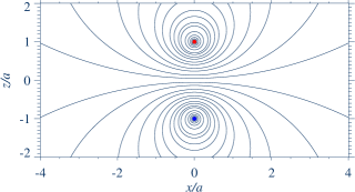
(a) A magnetically closed system: $z>0$

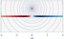
(b) Internal current system: $z>0$

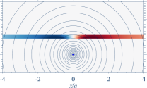
(c) External current system: $z<0$

Figure 2: The entangled origins of LABEL:sub@fig:BP12 the intrinsically solenoidal magnetic field $\boldsymbol{B}_{\mathrm{cl}}$ of a magnetically closed system for $z>0$ with $\hat{\boldsymbol{n}}\cdot\boldsymbol{B}_{\mathrm{cl}}|_{\partial\mathcal{V}}=0$ that is produced by two physical current systems: LABEL:sub@fig:BP:Internal one internal, $I\left(t\right)\,\hat{\boldsymbol{y}}$ at $x/a=0$ and $z/a=1$, and LABEL:sub@fig:BP:External one external, $-I\left(t\right)\,\hat{\boldsymbol{y}}$ at $x/a=0$ and $z/a=-1$. A red dot indicates a line current directed away from the observer and a blue dot indicates a line current towards the observer. The black lines are contours of the vector potential that trace magnetic field lines. The color scale along $z=0$ corresponds to the vertical magnetic field component with red/blue corresponding to up/down.

The physical implications of these boundary conditions are discussed in more detail in Appendix A. However, we touch on some obvious points here. First, $\partial\boldsymbol{A}/\partial t|_{\partial\mathcal{V}}=0$ implies that $\hat{\boldsymbol{n}}\cdot\partial\boldsymbol{B}/\partial t|_{\partial\mathcal{V}}=0$ but does not imply either $\hat{\boldsymbol{n}}\cdot\boldsymbol{J}|_{\partial\mathcal{V}}=0$ or $\hat{\boldsymbol{n}}\cdot\partial\boldsymbol{J}/\partial t|_{\partial\mathcal{V}}=0$—the two domains may share time-dependent current systems that pass through ${\partial\mathcal{V}}$. Second, hidden in Equation (16) is the assumption of gauge invariance which requires $\hat{\boldsymbol{n}}\cdot\boldsymbol{B}|_{\partial\mathcal{V}}=0$, e.g., $\hat{\boldsymbol{n}}\boldsymbol{\times}\boldsymbol{A}|_{\partial\mathcal{V}}=0$ to within a gauge transformation (see Appendix A). This is a stronger assumption than $\hat{\boldsymbol{n}}\cdot\partial\boldsymbol{B}/\partial t|_{\partial\mathcal{V}}=0$. Third, within the volume of interest $\mathcal{V}$, the magnetic field produced by “surface currents” is electrodynamically indistinguishable from the magnetic field produced by external currents $\boldsymbol{J}^{*}$ in ${\mathcal{V}^{*}}$. This last point suggests that even with the mathematical boundary conditions imposed by Woltjer (1958) that under special, albeit contrived, conditions, the motions in ${\mathcal{V}^{*}}$ can affect the magnetic field and plasma in $\mathcal{V}$. For example, consider the pedagogical system $\mathcal{V}$ and ${\mathcal{V}^{*}}$ bounded by ${\partial\mathcal{V}}$ at $z=0$ shown in Figure 2. The vector potential of this system is given by

$$A_{y}\left(t,x,z\right)=-\frac{I\left(t\right)}{c}\,\log\left[\frac{x^{2}+\left(z-a\right)^{2}}{x^{2}+\left(z+a\right)^{2}}\right],$$ (17)

where $I(t)$ is the current in the two thin, oppositely directed current channels at $x/a=0$ and $z/a=\pm 1$. The normal component, $B_{z}$, which is a superposition of these two current sources, has been contrived to precisely cancel at $z=0$, and $A_{y}(t,x,z=0)=0$ and thus $\mathcal{V}$ is a magnetically closed system by the mathematical boundary condition $\partial\boldsymbol{A}/\partial t|_{\partial\mathcal{V}}=0$ in Woltjer (1958). While there is no flux threading the boundary ${\partial\mathcal{V}}$ at $z=0$, Figure 2b shows that flux produced by the physical current source $I\left(t\right)\,\hat{\boldsymbol{y}}$ at $x/a=0$ and $z/a=1$ threads the boundary and permeates ${\mathcal{V}^{*}}$. Similarly Figure 2c shows that flux produced by the physical current source $-I\left(t\right)\,\hat{\boldsymbol{y}}$ at $x/a=0$ and $z/a=-1$ threads the boundary and permeates $\mathcal{V}$. The total magnetic field $\boldsymbol{B}\left(t,\boldsymbol{x}\right)$ for $\mathcal{V}$ shown in Figure 2a entangles the magnetic field from these two physical current sources and thus $\mathcal{V}$ and ${\mathcal{V}^{*}}$ are “communicating” in collusion to satisfy $B_{z}=0$ at $z=0$. This system results in the apparent non-sequitur that there can be magnetic field in $\mathcal{V}$ produced by currents $\boldsymbol{J}^{*}$ in ${\mathcal{V}^{*}}$ and magnetic field in ${\mathcal{V}^{*}}$ produced by currents $\boldsymbol{J}$ in $\mathcal{V}$ when no magnetic flux threads ${\partial\mathcal{V}}$, the boundary between $\mathcal{V}$ and ${\mathcal{V}^{*}}$. Of course this highly idealized system is not in force balance and is likely to relax violently to a lower energy state. Nonetheless, this example serves to demonstrate that a magnetically ‘closed’ system is not necessarily electrodynamically isolated and may be implicitly coupled to the external universe. A magnetically closed system may contain magnetic field produced by the external universe. Furthermore, the collusion between $\mathcal{V}$ and ${\mathcal{V}^{*}}$ described here is in common use in solar physics. It is analogous to the collusion between $\mathcal{V}$ and ${\mathcal{V}^{*}}$ required to impose flux preserving boundary conditions ($\hat{\boldsymbol{n}}\cdot\partial\boldsymbol{B}/\partial t|_{\partial\mathcal{V}}=0$) on the photosphere in photosphere-to-corona MHD simulations of the solar atmosphere (e.g., Kusano et al., 1995; Knizhnik et al., 2017; Linan et al., 2020; Bian & Jiang, 2023). We remark that the remainder of this paper is devoted to understanding the situation where two systems $\mathcal{V}$ and ${\mathcal{V}^{*}}$ are magnetically open and manifestly electrodynamically coupled.

Woltjer (1958) further showed that a force-free field $\boldsymbol{J}=\lambda\,\boldsymbol{B}$ with constant $\lambda$ represents the lowest state of magnetic energy that a magnetically closed system containing an ideal plasma can achieve while constrained by a prescribed helicity $H$. However, there was no obvious pathway for an ideal plasma to relax to the Woltjer state, because the equations of motion for an ideal MHD plasma exhibit an infinite number of symmetries corresponding to dynamical invariants, by Noether’s (1918) first theorem Frenkel et al. (1982). Thus, while the magnetic helicity, $H$, is preserved in an ideal plasma, it is not particularly unique or useful for describing ideal plasma dynamics—it is invariant, but it is just one of the infinity of invariants. The situation is different for a non-ideal plasma because Taylor (1974) conjectured that the magnetic helicity $H$ remains invariant even in the presence of weak dissipation which destroys the conservation of the other quantities. The Taylor conjecture provided a pathway for a closed system containing a near-ideal plasma to relax to the Woltjer linear force-free state while constrained by a prescribed helicity $H$. Helicity is a so-called “robust invariant,” meaning that it is approximately preserved during a rapid plasma relaxation to a lower energy state even if that involves dissipation, reconnection, and magnetic reorganization. Thus, while challenging to quantify, the magnetic helicity is an important measure of magnetic complexity in a near-ideal plasma.

4 Relative Helicity for Magnetically ‘Open’ Systems

The concept of helicity was then extended, by Berger & Field (1984) and Finn & Antonsen (1985), from magnetically ‘closed’ systems where magnetic “communication” is limited to current systems $\boldsymbol{J}$ in $\mathcal{V}$ and $\boldsymbol{J}^{*}$ in ${\mathcal{V}^{*}}$ that act in collusion to preserve $\hat{\boldsymbol{n}}\cdot\boldsymbol{B}|_{\partial\mathcal{V}}=0$ to magnetically ‘open’ systems where magnetic communication is manifest because magnetic flux threads the boundary ${\partial\mathcal{V}}$ and $\boldsymbol{J}$ in $\mathcal{V}$ and $\boldsymbol{J}^{*}$ in ${\mathcal{V}^{*}}$ can each independently contribute to $\hat{\boldsymbol{n}}\cdot\boldsymbol{B}|_{\partial\mathcal{V}}$. In this context, the helicity is measured relative to a reference magnetic field $\boldsymbol{B}_{\mathrm{R}}$ which threads the boundary ${\partial\mathcal{V}}$ of $\mathcal{V}$ in the same way as the magnetic field $\boldsymbol{B}$. Irregardless, for either open or closed systems, the linkages produced by currents in the external universe ${\mathcal{V}^{*}}$ can become entangled with the linkages produced by currents in the internal volume $\mathcal{V}$. The goal of this paper is to extend the work of Woltjer (1958), Berger & Field (1984), Finn & Antonsen (1985), and Berger (1999, 2003) and provide a clear distinction between the origin of the linkages in $\mathcal{V}$.

The relative magnetic helicity measure for systems supporting magnetic fields that thread the boundary ${\partial\mathcal{V}}$ proposed by Berger & Field (1984) and Finn & Antonsen (1985) is

$$\mathcal{H}=\int\limits_{\mathcal{V}}{d^{3}x}\left(\boldsymbol{A}+\boldsymbol{A}_{\mathrm{R}}\right)\cdot\left(\boldsymbol{B}-\boldsymbol{B}_{\mathrm{R}}\right),$$ (18)

where the reference magnetic field $\boldsymbol{B}_{\mathrm{R}}$ that threads the boundary ${\partial\mathcal{V}}$ is defined as

$$\boldsymbol{B}_{\mathrm{R}}=\boldsymbol{\nabla}\boldsymbol{\times}\boldsymbol{A}_{\mathrm{R}}\qquad\mbox{where}\qquad\left.\left(\boldsymbol{B}-\boldsymbol{B}_{\mathrm{R}}\right)\cdot\hat{\boldsymbol{n}}\right|_{\partial\mathcal{V}}=0,$$ (19)

and the magnetic field that closes in $\mathcal{V}$ is then defined as

$$\boldsymbol{A}_{\mathrm{cl}}= \boldsymbol{A}-\boldsymbol{A}_{\mathrm{R}},$$ (20a)

$$\boldsymbol{B}_{\mathrm{cl}}= \boldsymbol{B}-\boldsymbol{B}_{\mathrm{R}}=\boldsymbol{\nabla}\boldsymbol{\times}\boldsymbol{A}_{\mathrm{cl}}.$$ (20b)

The reference field represents the ‘open’ magnetic field that threads ${\partial\mathcal{V}}$ because $\hat{\boldsymbol{n}}\cdot\boldsymbol{B}_{\mathrm{R}}$ is nonzero on ${\partial\mathcal{V}}$, i.e., $\boldsymbol{B}_{\mathrm{R}}$ has components that enter and leave $\mathcal{V}$. The magnetic field $\boldsymbol{B}_{\mathrm{cl}}$ is solenoidal $\boldsymbol{\nabla}\cdot\boldsymbol{B}_{\mathrm{cl}}=0$, closes on itself in $\mathcal{V}$, and thus exhibits no normal component on ${\partial\mathcal{V}}$—it is an intrinsically solenoidal vector field in $\mathcal{V}$ Kemmer (1977); Schuck & Antiochos (2019). Note that expression (18) is gauge invariant because any gauge transformation of $\boldsymbol{A}$ or $\boldsymbol{A}_{\mathrm{R}}$ will involve the integral of the dot product between the gradient of a scalar $\boldsymbol{\nabla}\Lambda$ and an intrinsically solenoidal vector $\boldsymbol{B}-\boldsymbol{B}_{\mathrm{R}}$ that is tangent to ${\partial\mathcal{V}}$ and perpendicular to $\hat{\boldsymbol{n}}$ on ${\partial\mathcal{V}}$

$$\mathcal{H}\rightarrow\mathcal{H}+\int\limits_{\mathcal{V}}{d^{3}x}\,\boldsymbol{\nabla}\Lambda\cdot\left(\boldsymbol{B}-\boldsymbol{B}_{\mathrm{R}}\right)=\mathcal{H}-\oint\limits_{\partial\mathcal{V}}{dS}\,\hat{\boldsymbol{n}}\cdot\left[\Lambda\,\left(\boldsymbol{B}-\boldsymbol{B}_{\mathrm{R}}\right)\right]=\mathcal{H}.$$ (21)

All of the helicity terms developed in §5 have the analogous form and are similarly gauge invariant.

The potential magnetic field $\boldsymbol{P}$ is often used as a convenient reference field $\boldsymbol{B}_{\mathrm{R}}$. The potential field is harmonic and thus admits a dual representation in terms of a vector potential or in terms of the gradient of a scalar field

$$\boldsymbol{B}_{\mathrm{R}}\equiv\boldsymbol{P}=\boldsymbol{\nabla}\boldsymbol{\times}\boldsymbol{A}_{\mathrm{P}}=-\boldsymbol{\nabla}\psi\qquad\boldsymbol{x}\in\mathcal{V},$$ (22a)

which satisfies

$$\boldsymbol{\nabla}\boldsymbol{\times}\boldsymbol{P}=\boldsymbol{\nabla}\boldsymbol{\times}\boldsymbol{\nabla}\boldsymbol{\times}\boldsymbol{A}_{\mathrm{P}}=-\boldsymbol{\nabla}\boldsymbol{\times}\boldsymbol{\nabla}\psi=0 \qquad\boldsymbol{x}\in\mathcal{V},\qquad(\mbox{No Currents})$$ (22b)

$$\boldsymbol{\nabla}\cdot\boldsymbol{P}=\boldsymbol{\nabla}\cdot\boldsymbol{\nabla}\boldsymbol{\times}\boldsymbol{A}_{\mathrm{P}}=\nabla^{2}\psi=0 \qquad\boldsymbol{x}\in\mathcal{V}.\qquad(\mbox{No Monopoles})$$ (22c)

A unique solution for the vector potential, $$\boldsymbol{A}_{\mathrm{P}}$$, requires an arbitrary gauge condition for which the Coulomb gauge is a convenient choice (see Theorem 3.5 and Equations (3.23)-(3.25) in Girault & Raviart, 1986)

$$\boldsymbol{\nabla}\cdot\boldsymbol{A}_{\mathrm{P}}=0\quad\boldsymbol{x}\in\mathcal{V}\quad\mbox{and}\quad\hat{\boldsymbol{n}}\cdot\boldsymbol{A}_{\mathrm{P}}=0\quad\boldsymbol{x}\in{\partial\mathcal{V}},$$ (22d)

and with this gauge choice, the vector potential satisfies the vector Poisson equation

$$\nabla^{2}\boldsymbol{A}_{\mathrm{P}}=0\qquad\boldsymbol{x}\in\mathcal{V},$$ (22e)

with boundary condition

$$\hat{\boldsymbol{n}}\cdot\boldsymbol{B}=\hat{\boldsymbol{n}}\cdot\boldsymbol{\nabla}\boldsymbol{\times}\boldsymbol{A}_{\mathrm{P}}=-\hat{\boldsymbol{n}}\cdot\boldsymbol{\nabla}\psi\qquad\boldsymbol{x}\in{\partial\mathcal{V}}.$$ (22f)

Note that Equations (22c) and (22f) define the Neumann problem for the scalar potential $\psi$ which is unique to within an arbitrary scalar $\psi_{0}$ and Equations (22d)-(22f) define a unique vector potential for the same potential field $\boldsymbol{P}$. The field $\boldsymbol{P}$ is also the unique potential field that matches the normal component of $\boldsymbol{B}$ on the boundary ${\partial\mathcal{V}}$. A reference field $\boldsymbol{B}_{\mathrm{R}}$ that is potential is ‘convenient’ because no currents are supported by the potential field $\boldsymbol{P}$ in the volume of interest and thus the helicity of $\boldsymbol{B}_{\mathrm{R}}=\boldsymbol{P}$ in a simply connected domain may be intuitively defined as zero Berger (1999). However, as noted in the Introduction (§1), this convenience comes at the price of possibly misrepresenting the origin of the fields. Foreshadowing the development of §5, while $\boldsymbol{P}$ supports no internal currents in $\mathcal{V}$, Equation (22b) should not be interpreted to imply that $\boldsymbol{P}$ is produced exclusively by external currents! For example see Figure 1. Furthermore, while $\boldsymbol{B}_{\mathrm{cl}}$ supports the internal currents $\boldsymbol{J}$ in $\mathcal{V}$, it is generally produced by both these internal currents and by external currents $\boldsymbol{J}^{*}$ in ${\mathcal{V}^{*}}$. For example see Figure 2. This will be expanded on further in §5.2. In particular, non-potential magnetic fields in $\mathcal{V}$ can be produced by currents $\boldsymbol{J}^{*}$ in the external universe ${\mathcal{V}^{*}}$ when these currents thread the boundary ${\partial\mathcal{V}}$ to enter and leave $\mathcal{V}$. We emphasize that $\boldsymbol{B}=\boldsymbol{B}_{\mathrm{cl}}+\boldsymbol{P}$ is a mathematical decomposition determined by the geometry of the bounding surface ${\partial\mathcal{V}}$ that has no unique relationship with the origin of the magnetic field in currents.

Berger & Field (1984) showed that the evolution of the relative magnetic helicity for an ideal plasma depends only on boundary terms that may be computed from observables

$$\frac{d\mathcal{H}}{dt}=\frac{\partial}{\partial t}\int\limits_{\mathcal{V}}{d^{3}x}\left(\boldsymbol{A}+\boldsymbol{A}_{\mathrm{P}}\right)\cdot\left(\boldsymbol{B}-\boldsymbol{P}\right)=-2\,c\,\oint\limits_{\partial\mathcal{V}}{dS}\,\hat{\boldsymbol{n}}\cdot\boldsymbol{A}_{\mathrm{PC}}\boldsymbol{\times}\boldsymbol{E},$$ (23)

where $\boldsymbol{\nabla}\cdot\boldsymbol{A}_{\mathrm{PC}}=0$ in $\mathcal{V}$ is explicitly in the Coulomb gauge and the electric field $\boldsymbol{E}=-\boldsymbol{v}\boldsymbol{\times}\boldsymbol{B}/c$ is determined from the ideal Ohm’s law. Berger (1984) further argued that this relative helicity $\mathcal{H}$ is a robust invariant for finite volumes such as those enclosing flaring magnetic fields in the solar corona. A linear force-free field is the absolute minimum energy state of a plasma in volume $\mathcal{V}$ with a prescribed relative helicity $\mathcal{H}$ and a specified or ‘line-tied’ magnetic boundary $\left.\hat{\boldsymbol{n}}\cdot\boldsymbol{B}\right|_{\partial\mathcal{V}}=g\left(\boldsymbol{x}\right)$ condition Berger & Field (1984); Berger (1985); Jensen & Chu (1984); Dixon et al. (1989); Laurence & Avellaneda (1991).

Berger (1999, 2003) partitioned the relative helicity in Equation (18) into two further gauge invariant topological quantities: the closed-closed helicity $\mathcal{H}_{\mathrm{cl}}^{\mathrm{cl}}$ representing the linkages of magnetic field that closes in $\mathcal{V}$, and the open-closed helicity $\mathcal{H}_{\mathrm{cl}}^{\mathrm{o}}$ representing the linkages between the open magnetic field that threads the boundary ${\partial\mathcal{V}}$ and the magnetic field that closes inside $\mathcal{V}$:

$$\mathcal{H}=\int\limits_{\mathcal{V}}{d^{3}x}\,\underbrace{\overbrace{\left(\boldsymbol{A}-\boldsymbol{A}_{\mathrm{P}}\right)}^{\boldsymbol{A}_{\mathrm{cl}}}\cdot\overbrace{\left(\boldsymbol{B}-\boldsymbol{P}\right)}^{\boldsymbol{B}_{\mathrm{cl}}}}_{\mathcal{H}_{\mathrm{cl}}^{\mathrm{cl}}}+2\,\int\limits_{\mathcal{V}}{d^{3}x}\,\underbrace{\boldsymbol{A}_{\mathrm{P}}\cdot\overbrace{\left(\boldsymbol{B}-\boldsymbol{P}\right)}^{\boldsymbol{B}_{\mathrm{cl}}}}_{\mathcal{H}_{\mathrm{cl}}^{\mathrm{o}}},$$ (24)

where the Neumann potential magnetic field $\boldsymbol{P}$ has been implemented as the reference field $\boldsymbol{B}_{\mathrm{R}}$. Recently Pariat et al. (2017) (see also Moraitis et al., 2014; Linan et al., 2018; Zuccarello et al., 2018) have suggested that dynamic changes in the closed-closed helicity $\mathcal{H}_{\mathrm{cl}}^{\mathrm{cl}}$ may be a useful diagnostic of latent solar eruptivity leading to flares and coronal mass ejections. Pariat et al. (2017) denotes the first term in (24) $\mathcal{H}_{J}$ and designates it the “current carrying helicity” and denotes the second term $\mathcal{H}_{\mathrm{P}J}$ and designates it the “mutual helicity.”

There is nothing physically special about the linkages that close on themselves in $\mathcal{V}$ versus those that thread the boundary ${\partial\mathcal{V}}$: these fields are defined relative to a surface ${\partial\mathcal{V}}$ which often conveniently contains part of the photosphere in solar observational investigations where magnetic field data is regularly estimated from remote sensing observations, e.g., SDO/HMI. In other words, $\boldsymbol{P}$ and $\boldsymbol{B}_{\mathrm{cl}}$ are unique and topologically distinct only in the context of the field $\boldsymbol{B}$ and the volume $\mathcal{V}$ or equivalently ${\partial\mathcal{V}}$. A different volume $\mathcal{V}^{\prime}$ bounded by a different surface ${\partial\mathcal{V}}^{\prime}$ will lead to different potential fields $\boldsymbol{P}^{\prime}\neq\boldsymbol{P}$ and magnetic fields $\boldsymbol{B}_{\mathrm{cl}}^{\prime}\neq\boldsymbol{B}_{\mathrm{cl}}$ that close in $\mathcal{V}^{\prime}$ bounded by ${\partial\mathcal{V}}^{\prime}$, but the same total $\boldsymbol{B}=\boldsymbol{P}+\boldsymbol{B}_{\mathrm{cl}}=\boldsymbol{P}^{\prime}+\boldsymbol{B}_{\mathrm{cl}}^{\prime}$, at the same location $\boldsymbol{x}\in\mathcal{V}\cap\mathcal{V}^{\prime}$. The local force $\boldsymbol{J}\boldsymbol{\times}\boldsymbol{B}$ on the plasma is ultimately produced by the total magnetic field which contains no information about the boundary ${\partial\mathcal{V}}$, thus the magnetic field may be decomposed in whatever way is convenient to identify the magnetic topology and/or physical processes involved in the evolution of the plasma.

5 Relative Helicity with Attribution for Magnetically ‘Open’ Systems

Berger & Field (1984) and Finn & Antonsen (1985) established the relative helicity $\mathcal{H}$ as a gauge invariant measure of magnetic complexity in magnetically open systems. The potential field $\boldsymbol{P}$ is a convenient reference field as, mathematically, the origin of $\boldsymbol{P}$ is in currents supported by the external universe ${\mathcal{V}^{*}}$—hence its helicity $\int_{\mathcal{V}}{d^{3}x}\,\boldsymbol{A}_{\mathrm{P}}\cdot\boldsymbol{P}$ in $\mathcal{V}$ may be defined as zero in a simply connected domain Berger (1999). However, as noted in Schuck et al. (2022) and §1 and §2 here, the physical origin of potential field may be in current supported in $\mathcal{V}$. Thus the potential field $\boldsymbol{P}$ can misattribute the origin of flux threading the bounding surface to external current sources. This insight suggests that Berger’s decomposition of helicity in Equation (24) may be further disentangled when the origin of the magnetic field in currents is considered. The Berger & Field (1984) and Finn & Antonsen (1985) formula (18) is convenient for describing the attribution of helicity because it is gauge agnostic—we are free to write $\boldsymbol{A}$ and $\boldsymbol{A}_{\mathrm{R}}$ in any gauge. Below in §5.1-5.3 we extend Berger’s decomposition of relative helicity in Equation (24) to include attribution of the fields to their current sources in $\mathcal{V}$ and ${\mathcal{V}^{*}}$. This motivates new definitions of internal and external and internal-external relative helicity distinguished by the domain of the current system that produces the magnetic linkages. Our presentation is general in that it is easily extended mutatis mutandis to a coronal volume bounded by the photosphere and a boundary in the high corona or a box of length $L$ on a side.

5.1 Internal Relative Helicity in $\mathcal{V}$ Produced by Internal Sources: $\boldsymbol{J}$ in $\mathcal{V}$

To compute the internal relative helicity produced by internal sources we need to construct the field pairs $\left(\boldsymbol{A},\boldsymbol{B}\right)$ and $\left(\boldsymbol{A}_{\mathrm{P}},\boldsymbol{P}\right)$ produced by internal sources $\boldsymbol{J}$. For the current system $\boldsymbol{J}$ in the domain of interest $\mathcal{V}$ the vector potential and magnetic field follows directly from Equation (4b)

$$\boldsymbol{A}\left(\boldsymbol{J};t,\boldsymbol{x}\right)\equiv \frac{1}{c}\,\int\limits_{\mathcal{V}}{d^{3}x^{\prime}}\,\frac{\boldsymbol{J}\left(t,\boldsymbol{x}^{\prime}\right)}{\left|\boldsymbol{x}-\boldsymbol{x}^{\prime}\right|}\qquad \boldsymbol{x}\in{\mathbb{R}^{3}},$$ (25a)

$$\boldsymbol{B}_{\mathrm{BS}}\left(\boldsymbol{J};t,\boldsymbol{x}\right)\equiv \boldsymbol{\nabla}\boldsymbol{\times}\boldsymbol{A}\left(\boldsymbol{J};t,\boldsymbol{x}\right)\qquad \boldsymbol{x}\in{\mathbb{R}^{3}},$$ (25b)

which completely describes the attribution of the vector potential and magnetic field produced by currents $\boldsymbol{J}$ in $\mathcal{V}$. This field integrant may be decomposed in the usual fashion into magnetic fields that close in $\mathcal{V}$ and magnetic fields that thread the boundary ${\partial\mathcal{V}}$ using the potential field methodology described above in Equations (22a)-(22f). Explicitly this is

$$\boldsymbol{P}\left(\boldsymbol{J};t,\boldsymbol{x}\right)= \boldsymbol{\nabla}\boldsymbol{\times}\boldsymbol{A}_{\mathrm{P}}\left(\boldsymbol{J};t,\boldsymbol{x}\right)\quad\mbox{and}\quad\boldsymbol{P}\left(\boldsymbol{J};t,\boldsymbol{x}\right)=-\boldsymbol{\nabla}\psi\left(\boldsymbol{J};t,\boldsymbol{x}\right)\qquad \boldsymbol{x}\in\mathcal{V},$$ (26a)

$$\boldsymbol{\nabla}\cdot\boldsymbol{A}_{\mathrm{P}}\left(\boldsymbol{J};t,\boldsymbol{x}\right)= 0\quad\boldsymbol{x}\in\mathcal{V}\quad\mbox{and}\quad\hat{\boldsymbol{n}}\cdot\boldsymbol{A}_{\mathrm{P}}\left(\boldsymbol{J};t,\boldsymbol{x}\right)=0\quad \boldsymbol{x}\in{\partial\mathcal{V}},$$ (26b)

$$\nabla^{2}\boldsymbol{A}_{\mathrm{P}}\left(\boldsymbol{J};t,\boldsymbol{x}\right)= 0\quad\mbox{and}\quad\nabla^{2}\psi\left(\boldsymbol{J};t,\boldsymbol{x}\right)=0\qquad \boldsymbol{x}\in\mathcal{V},$$ (26c)

$$\hat{\boldsymbol{n}}\cdot\boldsymbol{B}_{\mathrm{BS}}\left(\boldsymbol{J};t,\boldsymbol{x}\right)= \hat{\boldsymbol{n}}\cdot\boldsymbol{\nabla}\boldsymbol{\times}\boldsymbol{A}_{\mathrm{P}}\left(\boldsymbol{J};t,\boldsymbol{x}\right)=-\hat{\boldsymbol{n}}\cdot\boldsymbol{\nabla}\psi\left(\boldsymbol{J};t,\boldsymbol{x}\right)\qquad \boldsymbol{x}\in{\partial\mathcal{V}}.$$ (26d)

Note that Equations (26a)-(26d) differ from (22a), and (22d)-(22f) in that the former represents the potential field produced on the boundary by physically internal sources and the latter represents the potential field produced on the boundary by all physical sources (internal and external). This distinction is imposed by the boundary conditions (26d) and (22f), which in the former case is determined by the normal component of the Biot-Savart law integrated over just the internal sources $\boldsymbol{J}$ and in the latter case by the total field $\boldsymbol{B}$.

The magnetic fields that close in $\mathcal{V}$ and are produced by internal current sources in $\mathcal{V}$ are then described as

$$\boldsymbol{A}_{\mathrm{cl}}\left(\boldsymbol{J};t,\boldsymbol{x}\right)\equiv \boldsymbol{A}\left(\boldsymbol{J};t,\boldsymbol{x}\right)-\boldsymbol{A}_{\mathrm{P}}\left(\boldsymbol{J};t,\boldsymbol{x}\right),$$ (27a)

$$\boldsymbol{B}_{\mathrm{cl}}\left(\boldsymbol{J};t,\boldsymbol{x}\right)\equiv \boldsymbol{B}_{\mathrm{BS}}\left(\boldsymbol{J};t,\boldsymbol{x}\right)-\boldsymbol{P}\left(\boldsymbol{J};t,x\right),$$

$$= \boldsymbol{\nabla}\boldsymbol{\times}\boldsymbol{A}_{\mathrm{cl}}\left(\boldsymbol{J};t,\boldsymbol{x}\right)=\boldsymbol{\nabla}\boldsymbol{\times}\left[\boldsymbol{A}\left(\boldsymbol{J};t,\boldsymbol{x}\right)-\boldsymbol{A}_{\mathrm{P}}\left(\boldsymbol{J};t,\boldsymbol{x}\right)\right].$$ (27b)

The internal relative helicity which corresponds to the internal current sources is then

$$\mathcal{H}\left(\boldsymbol{J},\boldsymbol{J}\right)=\underbrace{\int_{\mathcal{V}}{d^{3}x}\,\overbrace{\left[\boldsymbol{A}\left(\boldsymbol{J}\right)-\boldsymbol{A}_{\mathrm{P}}\left(\boldsymbol{J}\right)\right]}^{\boldsymbol{A}_{\mathrm{cl}}\left(\boldsymbol{J}\right)}\cdot\overbrace{\left[\boldsymbol{B}_{\mathrm{BS}}\left(\boldsymbol{J}\right)-\boldsymbol{P}\left(\boldsymbol{J}\right)\right]}^{\boldsymbol{B}_{\mathrm{cl}}\left(\boldsymbol{J}\right)}}_{\mathcal{H}_{\mathrm{cl}}^{\mathrm{cl}}\left(\boldsymbol{J},\boldsymbol{J}\right)}+\underbrace{2\,\int_{\mathcal{V}}{d^{3}x}\,\boldsymbol{A}_{\mathrm{P}}\left(\boldsymbol{J}\right)\cdot\overbrace{\left[\boldsymbol{B}_{\mathrm{BS}}\left(\boldsymbol{J}\right)-\boldsymbol{P}\left(\boldsymbol{J}\right)\right]}^{\boldsymbol{B}_{\mathrm{cl}}\left(\boldsymbol{J}\right)}}_{\mathcal{H}_{\mathrm{cl}}^{\mathrm{o}}\left(\boldsymbol{J},\boldsymbol{J}\right)},$$ (28)

where the independent variables $t$ and $\boldsymbol{x}$ have been suppressed for brevity. Both integrals are gauge invariant because $\boldsymbol{\nabla}\cdot\boldsymbol{B}_{\mathrm{cl}}\left(\boldsymbol{J}\right)=0$ and $\hat{\boldsymbol{n}}\cdot\left.\boldsymbol{B}_{\mathrm{cl}}\left(\boldsymbol{J}\right)\right|_{\partial\mathcal{V}}=0$ by construction (see Equation (21)). In the Berger (1999, 2003) paradigm, this expression describes the closed-closed helicity $\mathcal{H}_{\mathrm{cl}}^{\mathrm{cl}}\left(\boldsymbol{J},\boldsymbol{J}\right)$ of the magnetic field that is produced by internal current sources and closes in $\mathcal{V}$ and the open-closed helicity $\mathcal{H}_{\mathrm{cl}}^{\mathrm{o}}\left(\boldsymbol{J},\boldsymbol{J}\right)$ between the magnetic field that is produced by internal current sources and closes in $\mathcal{V}$ and the magnetic field that is produced by internal current sources and threads the boundary ${\partial\mathcal{V}}$. However, in our new paradigm $\mathcal{H}\left(\boldsymbol{J},\boldsymbol{J}\right)$ represents the total internal relative helicity in $\mathcal{V}$ of magnetic field produced by currents $\boldsymbol{J}$ in $\mathcal{V}$. This is arguably the true self-helicity of the current system $\boldsymbol{J}$ in $\mathcal{V}$. If there were no external currents $\boldsymbol{J}^{*}$, then Equations (24) and (28) would produce identical values.

5.2 External Relative Helicity in $\mathcal{V}$ Produced by External Sources: $\boldsymbol{J}^{*}$ in ${\mathcal{V}^{*}}$

To compute the external relative helicity produced by external sources we need to construct the field pairs $\left(\boldsymbol{A},\boldsymbol{B}\right)$ and $\left(\boldsymbol{A}_{\mathrm{P}},\boldsymbol{P}\right)$ produced by external sources $\boldsymbol{J}^{*}$. The magnetic vector potential $\boldsymbol{A}$ and corresponding magnetic field $\boldsymbol{B}$ produced by external current sources follows directly from (4c)

$$\boldsymbol{A}\left(\boldsymbol{J}^{*};t,\boldsymbol{x}\right)\equiv \frac{1}{c}\,\int\limits_{{\mathcal{V}^{*}}}{d^{3}x^{\prime}}\,\frac{\boldsymbol{J}^{*}\left(t,\boldsymbol{x}^{\prime}\right)}{\left|\boldsymbol{x}-\boldsymbol{x}^{\prime}\right|}\qquad \boldsymbol{x}\in{\mathbb{R}^{3}},$$ (29a)

$$\boldsymbol{B}_{\mathrm{BS}}\left(\boldsymbol{J}^{*};t,\boldsymbol{x}\right)\equiv \boldsymbol{\nabla}\boldsymbol{\times}\boldsymbol{A}\left(\boldsymbol{J}^{*};t,\boldsymbol{x}\right)\qquad \boldsymbol{x}\in{\mathbb{R}^{3}},$$ (29b)

where the domain of integration is over the entire external volume ${\mathcal{V}^{*}}$ that contains current sources $\boldsymbol{J}^{*}$. However, in practice, we do not have access to this information. Usually, at best, we have information about the currents $\boldsymbol{J}$ in our domain of interest $\mathcal{V}$ and information on the boundary ${\partial\mathcal{V}}$ and so while Equations (29a)-(29b) are formally correct and useful for developing insight, they are not practical for computation. However, the magnetic field due to external sources can be computed from (13a)-(13b). We emphasize again here that determining $\boldsymbol{B}_{\mathrm{BS}}\left(\boldsymbol{J}^{*};t,\boldsymbol{x}\right)$ in $\mathcal{V}$ does not require performing the Biot-Savart integral over $\boldsymbol{J}^{*}$ in ${\mathcal{V}^{*}}$.

Again, this field may be decomposed in the usual fashion into magnetic fields that close in $\mathcal{V}$ and magnetic fields that thread the boundary ${\partial\mathcal{V}}$ using the potential field methodology described above in equations (22a)-(22f). Explicitly this is

$$\boldsymbol{P}\left(\boldsymbol{J}^{*};t,\boldsymbol{x}\right)= \boldsymbol{\nabla}\boldsymbol{\times}\boldsymbol{A}_{\mathrm{P}}\left(\boldsymbol{J}^{*};t,\boldsymbol{x}\right)\quad\mbox{and}\quad\boldsymbol{P}\left(\boldsymbol{J}^{*};t,\boldsymbol{x}\right)=-\boldsymbol{\nabla}\psi\left(\boldsymbol{J}^{*};t,\boldsymbol{x}\right)\qquad \boldsymbol{x}\in\mathcal{V},$$ (30a)

$$\boldsymbol{\nabla}\cdot\boldsymbol{A}_{\mathrm{P}}\left(\boldsymbol{J}^{*};t,\boldsymbol{x}\right)= 0\quad\boldsymbol{x}\in\mathcal{V}\quad\mbox{and}\quad\hat{\boldsymbol{n}}\cdot\boldsymbol{A}_{\mathrm{P}}\left(\boldsymbol{J}^{*};t,\boldsymbol{x}\right)=0\quad \boldsymbol{x}\in{\partial\mathcal{V}},$$ (30b)

$$\nabla^{2}\boldsymbol{A}_{\mathrm{P}}\left(\boldsymbol{J}^{*};t,\boldsymbol{x}\right)= 0\quad\mbox{and}\quad\nabla^{2}\psi\left(\boldsymbol{J}^{*};t,\boldsymbol{x}\right)=0\qquad \boldsymbol{x}\in\mathcal{V},$$ (30c)

$$\hat{\boldsymbol{n}}\cdot\boldsymbol{B}_{\mathrm{BS}}\left(\boldsymbol{J}^{*};t,\boldsymbol{x}\right)= \hat{\boldsymbol{n}}\cdot\boldsymbol{\nabla}\boldsymbol{\times}\boldsymbol{A}_{\mathrm{P}}\left(\boldsymbol{J}^{*};t,\boldsymbol{x}\right)=-\hat{\boldsymbol{n}}\cdot\boldsymbol{\nabla}\psi\left(\boldsymbol{J}^{*};t,\boldsymbol{x}\right)\qquad \boldsymbol{x}\in{\partial\mathcal{V}}.$$ (30d)

Combining the results in Equations (22a), (26a) and (30a), and making use of Equations (22f), (26d), (30d), and (4a),

$$\psi\left(t,\boldsymbol{x}\right)=\psi\left(\boldsymbol{J};t,\boldsymbol{x}\right)+\psi\left(\boldsymbol{J}^{*};t,\boldsymbol{x}\right)\qquad\boldsymbol{x}\in\mathcal{V},$$ (31)

or

$$\boldsymbol{P}\left(t,\boldsymbol{x}\right)=\boldsymbol{P}\left(\boldsymbol{J};t,\boldsymbol{x}\right)+\boldsymbol{P}\left(\boldsymbol{J}^{*};t,\boldsymbol{x}\right)\qquad\boldsymbol{x}\in\mathcal{V},$$ (32)

and we see that the traditional Neumann potential field described by $\boldsymbol{P}=-\boldsymbol{\nabla}\psi$ conflates the magnetic field produced by internal current sources $\boldsymbol{J}$ and external current sources $\boldsymbol{J}^{*}$ as discussed in the introduction. A similar conflation occurs for the closed field $\boldsymbol{B}_{\mathrm{cl}}$. The closed field produced by external currents is

$$\boldsymbol{B}_{\mathrm{cl}}\left(\boldsymbol{J}^{*};t,x\right)=\boldsymbol{B}_{\mathrm{BS}}\left(\boldsymbol{J}^{*};t,\boldsymbol{x}\right)-\boldsymbol{P}\left(\boldsymbol{J}^{*};t,\boldsymbol{x}\right)\qquad\boldsymbol{x}\in\mathcal{V},$$ (33)

and then combining the results in Equations (20b),  (27b) and (33), and making use of Equations (22a), (4a), and (32),

$$\boldsymbol{B}_{\mathrm{cl}}\left(t,x\right)=\boldsymbol{B}_{\mathrm{cl}}\left(\boldsymbol{J};t,x\right)+\boldsymbol{B}_{\mathrm{cl}}\left(\boldsymbol{J}^{*};t,x\right)=\boldsymbol{B}\left(t,x\right)-\boldsymbol{P}\left(t,x\right)\qquad\boldsymbol{x}\in\mathcal{V}.$$ (34)

For the external current system $\boldsymbol{J}$ to contribute to the closed field $\boldsymbol{B}_{\mathrm{cl}}$ in $\mathcal{V}$ is perhaps not surprising given Figure 2. However, the external current system $\boldsymbol{J}^{*}$ in ${\mathcal{V}^{*}}$ can produce closed-closed helicity $\mathcal{H}_{\mathrm{cl}}^{\mathrm{cl}}$ in $\mathcal{V}$ by generating closed field in $\mathcal{V}$ on its own! The presence of current systems that pass from $\mathcal{V}$ to ${\mathcal{V}^{*}}$ or vice versa also implies that

$$\boldsymbol{\nabla}\boldsymbol{\times}\boldsymbol{B}_{\mathrm{cl}}\left(\boldsymbol{J}^{*};t,\boldsymbol{x}\right)\neq 0\qquad\boldsymbol{x}\in\mathcal{V}.$$ (35)

The external current, $\boldsymbol{J}^{*}$, in volume, ${\mathcal{V}^{*}}$, injects magnetic vorticity into $\mathcal{V}$. This is apparent if we consider the curl of (29b)

$$\boldsymbol{\nabla}\boldsymbol{\times}\boldsymbol{B}_{\mathrm{BS}}\left(\boldsymbol{J}^{*};t,\boldsymbol{x}\right)=\frac{1}{c}\,\boldsymbol{\nabla}\boldsymbol{\times}\boldsymbol{\nabla}\boldsymbol{\times}\int\limits_{{\mathcal{V}^{*}}}{d^{3}x^{\prime}}\,\frac{\boldsymbol{J}^{*}\left(t,\boldsymbol{x}^{\prime}\right)}{\left|\boldsymbol{x}-\boldsymbol{x}^{\prime}\right|}\qquad\boldsymbol{x}\in{\mathbb{R}^{3}},$$ (36)

where the observation point $\boldsymbol{x}$ is in $\mathcal{V}$ not ${\mathcal{V}^{*}}$. Using the vector relationship

$$\boldsymbol{\nabla}\boldsymbol{\times}\boldsymbol{\nabla}\boldsymbol{\times}\boldsymbol{a}=\boldsymbol{\nabla}\left(\boldsymbol{\nabla}\cdot\boldsymbol{a}\right)-\nabla^{2}\boldsymbol{a},$$ (37)

this becomes

$$\boldsymbol{\nabla}\boldsymbol{\times}\boldsymbol{B}_{\mathrm{BS}}\left(\boldsymbol{J}^{*};t,\boldsymbol{x}\right)=\frac{1}{c}\,\boldsymbol{\nabla}\left[\boldsymbol{\nabla}\cdot\int\limits_{{\mathcal{V}^{*}}}{d^{3}x^{\prime}}\,\frac{\boldsymbol{J}^{*}\left(t,\boldsymbol{x}^{\prime}\right)}{\left|\boldsymbol{x}-\boldsymbol{x}^{\prime}\right|}\right]-\frac{1}{c}\,\nabla^{2}\int\limits_{{\mathcal{V}^{*}}}{d^{3}x^{\prime}}\,\frac{\boldsymbol{J}^{*}\left(t,\boldsymbol{x}^{\prime}\right)}{\left|\boldsymbol{x}-\boldsymbol{x}^{\prime}\right|}\qquad\boldsymbol{x}\in{\mathbb{R}^{3}}.$$ (38)

The kernel in the second term has the form of a delta distribution because

$$\nabla^{2}\left|\boldsymbol{x}-\boldsymbol{x}^{\prime}\right|^{-1}=-4\,\pi\,\left\{\begin{array}[]{lr}\delta\left(\boldsymbol{x}-\boldsymbol{x}^{\prime}\right)&\boldsymbol{x}\in{\mathcal{V}^{*}},\\ \alpha^{*}\left(x\right)\,\delta\left(\boldsymbol{x}-\boldsymbol{x}^{\prime}\right)&\boldsymbol{x}\in{{\partial\mathcal{V}}^{*}},\\ 0&\boldsymbol{x}\in\mathcal{V}.\end{array}\right.$$ (39)

leading to

$$\boldsymbol{\nabla}\boldsymbol{\times}\boldsymbol{B}_{\mathrm{BS}}\left(\boldsymbol{J}^{*};t,\boldsymbol{x}\right)-\frac{1}{c}\,\boldsymbol{\nabla}\left[\boldsymbol{\nabla}\cdot\int\limits_{{\mathcal{V}^{*}}}{d^{3}x^{\prime}}\,\frac{\boldsymbol{J}^{*}\left(t,\boldsymbol{x}^{\prime}\right)}{\left|\boldsymbol{x}-\boldsymbol{x}^{\prime}\right|}\right]=\frac{4\,\pi}{c}\,\alpha^{*}\left(\boldsymbol{x}\right)\,\boldsymbol{J}^{*}\left(t,\boldsymbol{x}\right)\qquad\boldsymbol{x}\in{\mathbb{R}^{3}},$$ (40)

where

$$\alpha^{*}\left(\boldsymbol{x}\right)=1-\alpha\left(\boldsymbol{x}\right)=\left\{\begin{array}[]{ll}1&\boldsymbol{x}\in{\mathcal{V}^{*}}\\ \left.\begin{array}[]{ll}1/2&\mbox{smooth surfaces}\\ 3/4&\mbox{edges of $\mathcal{V}$}\\ 7/8&\mbox{vertices of $\mathcal{V}$}\end{array}\right\}&\boldsymbol{x}\in{{\partial\mathcal{V}}^{*}}\\ 0&\boldsymbol{x}\in\mathcal{V}\end{array}\right.,$$ (41)

follows from Equation (6b) for $\alpha\left(\boldsymbol{x}\right)$ and for the values in braces we have assumed that ${\mathcal{V}^{*}}$ encloses $\mathcal{V}$. Passing the divergence under the integral operator, using

$$\boldsymbol{\nabla}\frac{1}{\left|\boldsymbol{x}-\boldsymbol{x}^{\prime}\right|}=-\boldsymbol{\nabla}^{\prime}\frac{1}{\left|\boldsymbol{x}-\boldsymbol{x}^{\prime}\right|},$$ (42)

and

$$\boldsymbol{\nabla}\cdot\left(\phi\,\boldsymbol{a}\right)=\boldsymbol{a}\cdot\boldsymbol{\nabla}\phi+\phi\,\boldsymbol{\nabla}\cdot\boldsymbol{a},$$ (43)

this simplifies to

$$\boldsymbol{\nabla}\boldsymbol{\times}\boldsymbol{B}_{\mathrm{BS}}\left(\boldsymbol{J}^{*};t,\boldsymbol{x}\right)+\frac{1}{c}\,\boldsymbol{\nabla}\left[\int\limits_{{\mathcal{V}^{*}}}{d^{3}x^{\prime}}\,\boldsymbol{\nabla}^{\prime}\cdot\,\frac{\boldsymbol{J}^{*}\left(t,\boldsymbol{x}^{\prime}\right)}{\left|\boldsymbol{x}-\boldsymbol{x}^{\prime}\right|}-\int\limits_{{\mathcal{V}^{*}}}{d^{3}x^{\prime}}\,\frac{\boldsymbol{\nabla}^{\prime}\cdot\boldsymbol{J}^{*}\left(t,\boldsymbol{x}^{\prime}\right)}{\left|\boldsymbol{x}-\boldsymbol{x}^{\prime}\right|}\right]=\frac{4\,\pi}{c}\,\alpha^{*}\left(\boldsymbol{x}\right)\,\boldsymbol{J}^{*}\left(t,\boldsymbol{x}\right)\qquad\boldsymbol{x}\in{\mathbb{R}^{3}}.$$ (44)

The Gauss-Ostrogradsky theorem where $\hat{\boldsymbol{n}}$ points into $\mathcal{V}$

$$\int\limits_{\mathcal{V}}{d^{3}x}\,\boldsymbol{\nabla}\cdot\boldsymbol{a}=-\oint\limits_{{\partial\mathcal{V}}}{dS}\,\hat{\boldsymbol{n}}\cdot\boldsymbol{a},$$ (45)

relates the volume integral of the divergence to a surface integral over the normal component at the boundary of the volume. Then with the Gauss-Ostrogradsky theorem, Equation (44) becomes

$$\boldsymbol{\nabla}\boldsymbol{\times}\boldsymbol{B}_{\mathrm{BS}}\left(\boldsymbol{J}^{*};t,\boldsymbol{x}\right)-\frac{1}{c}\,\overbrace{\boldsymbol{\nabla}\left[\oint\limits_{{{\partial\mathcal{V}}^{*}}}{dS^{\prime}}\,\frac{\hat{\boldsymbol{n}}^{\prime}\cdot\boldsymbol{J}^{*}\left(t,\boldsymbol{x}^{\prime}\right)}{\left|\boldsymbol{x}-\boldsymbol{x}^{\prime}\right|}+\int\limits_{{\mathcal{V}^{*}}}{d^{3}x^{\prime}}\,\frac{\boldsymbol{\nabla}^{\prime}\cdot\boldsymbol{J}^{*}\left(t,\boldsymbol{x}^{\prime}\right)}{\left|\boldsymbol{x}-\boldsymbol{x}^{\prime}\right|}\right]}^{{\partial\boldsymbol{E}\left(\boldsymbol{J}^{*};t,\boldsymbol{x}\right)}/{\partial t}}=\frac{4\,\pi}{c}\,\alpha^{*}\left(\boldsymbol{x}\right)\,\boldsymbol{J}^{*}\left(t,\boldsymbol{x}\right)\qquad\boldsymbol{x}\in{\mathbb{R}^{3}},$$ (46a)

or with $$\boldsymbol{\nabla}\cdot\boldsymbol{J}^{*}=0 \boldsymbol{x}\in\mathcal{V}$$ for

$$\boldsymbol{\nabla}\boldsymbol{\times}\boldsymbol{B}_{\mathrm{BS}}\left(\boldsymbol{J}^{*};t,\boldsymbol{x}\right)+\frac{1}{c}\,\overbrace{\boldsymbol{\nabla}\oint\limits_{{\partial\mathcal{V}}}{dS^{\prime}}\,\frac{\hat{\boldsymbol{n}}^{\prime}\cdot\boldsymbol{J}\left(t,\boldsymbol{x}^{\prime}\right)}{\left|\boldsymbol{x}-\boldsymbol{x}^{\prime}\right|}}^{-{\partial\boldsymbol{E}\left(\boldsymbol{J}^{*};t,\boldsymbol{x}\right)}/{\partial t}}=0\qquad\boldsymbol{x}\in\mathcal{V}.$$ (46b)

where in the last expression we have taken the surface integral with respect to $${\partial\mathcal{V}} {{\partial\mathcal{V}}^{*}} \boldsymbol{\nabla}\cdot\boldsymbol{J}^{*}=0 \hat{\boldsymbol{n}}\cdot\left(\boldsymbol{J}-\boldsymbol{J}^{*}\right)=0 \boldsymbol{x}\in{\partial\mathcal{V}}$$ instead of , used as implied by Ampere’s law (8), and assumed that the normal component of the current is continuous across the boundary for . Equation (46b) has the form of the Ampère-Maxwell equation

$$\boldsymbol{\nabla}\boldsymbol{\times}\boldsymbol{B}_{\mathrm{BS}}\left(\boldsymbol{J}^{*};t,\boldsymbol{x}\right)-\frac{1}{c}\,\frac{\partial\boldsymbol{E}\left(\boldsymbol{J}^{*};t,\boldsymbol{x}\right)}{\partial t}=0\qquad\boldsymbol{x}\in\mathcal{V},$$ (46c)

where there is no external material current $\boldsymbol{J}^{*}$ in $\mathcal{V}$. Thus, the magnetic vorticity produced in $\mathcal{V}$ is balanced, but not generated, by a time-dependent electric field in $\mathcal{V}$, the so-called ‘displacement current,’ and both are produced by $\boldsymbol{J}^{*}$ in ${\mathcal{V}^{*}}$ or on ${\partial\mathcal{V}}$. We emphasize that the displacement current $\partial\boldsymbol{E}/\partial t$ is not a source of magnetic field. Closed magnetic field in the sense of $\oint\,\boldsymbol{B}\left(\boldsymbol{J}^{*};t,\boldsymbol{x}\right)\cdot{d\ell}\neq 0$ for $\boldsymbol{x}\in\mathcal{V}$, indicates the presence of magnetic vorticity—and not the exclusive presence of a local material current $\boldsymbol{J}$. The source of this magnetic vorticity in $\mathcal{V}$ may be a non-local current source, e.g., $\boldsymbol{J}^{*}$ in ${\mathcal{V}^{*}}$.

The presence of displacement currents must be reconciled with Ampére’s law (8). Consider $\boldsymbol{\nabla}\boldsymbol{\times}\boldsymbol{B}_{\mathrm{BS}}\left(\boldsymbol{J};t,\boldsymbol{x}\right)$ by following the derivation of (46a) mutatis mutandis

$$\boldsymbol{\nabla}\boldsymbol{\times}\boldsymbol{B}_{\mathrm{BS}}\left(\boldsymbol{J};t,\boldsymbol{x}\right)-\frac{1}{c}\,\overbrace{\boldsymbol{\nabla}\left[\oint\limits_{{\partial\mathcal{V}}}{dS^{\prime}}\,\hat{\boldsymbol{n}}^{\prime}\cdot\,\frac{\boldsymbol{J}\left(t,\boldsymbol{x}^{\prime}\right)}{\left|\boldsymbol{x}-\boldsymbol{x}^{\prime}\right|}+\int\limits_{\mathcal{V}}{d^{3}x^{\prime}}\,\frac{\boldsymbol{\nabla}^{\prime}\cdot\boldsymbol{J}\left(t,\boldsymbol{x}^{\prime}\right)}{\left|\boldsymbol{x}-\boldsymbol{x}^{\prime}\right|}\right]}^{{\partial\boldsymbol{E}\left(\boldsymbol{J};t,\boldsymbol{x}\right)}/{\partial t}}=\frac{4\,\pi}{c}\,\alpha\left(\boldsymbol{x}\right)\,\boldsymbol{J}\left(t,\boldsymbol{x}\right)\qquad\boldsymbol{x}\in{\mathbb{R}^{3}},$$ (47a)

or with $$\boldsymbol{\nabla}\cdot\boldsymbol{J}=0 \boldsymbol{x}\in\mathcal{V}$$ for

$$\boldsymbol{\nabla}\boldsymbol{\times}\boldsymbol{B}_{\mathrm{BS}}\left(\boldsymbol{J};t,\boldsymbol{x}\right)-\frac{1}{c}\,\overbrace{\boldsymbol{\nabla}\oint\limits_{{\partial\mathcal{V}}}{dS^{\prime}}\,\frac{\hat{\boldsymbol{n}}^{\prime}\cdot\boldsymbol{J}\left(t,\boldsymbol{x}^{\prime}\right)}{\left|\boldsymbol{x}-\boldsymbol{x}^{\prime}\right|}}^{{\partial\boldsymbol{E}\left(\boldsymbol{J};t,\boldsymbol{x}\right)}/{\partial t}}=\frac{4\,\pi}{c}\,\boldsymbol{J}\left(t,\boldsymbol{x}\right)\qquad\boldsymbol{x}\in\mathcal{V}.$$ (47b)

which has a material current because $$\nabla^{2}\left|\boldsymbol{x}-\boldsymbol{x}^{\prime}\right|^{-1}=-4\,\pi\,\delta\left(\boldsymbol{x}-\boldsymbol{x}^{\prime}\right) \boldsymbol{x}\in\mathcal{V} \boldsymbol{x}^{\prime}\in\mathcal{V}$$ is a delta distribution for and . This also has the form of the Ampère-Maxwell equation

$$\boldsymbol{\nabla}\boldsymbol{\times}\boldsymbol{B}_{\mathrm{BS}}\left(\boldsymbol{J};t,\boldsymbol{x}\right)-\frac{1}{c}\,\frac{\partial\boldsymbol{E}\left(\boldsymbol{J};t,\boldsymbol{x}\right)}{\partial t}=\frac{4\,\pi}{c}\,\boldsymbol{J}\left(t,\boldsymbol{x}\right)\qquad\boldsymbol{x}\in\mathcal{V}.$$ (47c)

Combining Equations (46a) and (47a)

$$\boldsymbol{\nabla}\boldsymbol{\times}\boldsymbol{B}_{\mathrm{BS}}\left(\boldsymbol{J};t,\boldsymbol{x}\right)+\boldsymbol{\nabla}\boldsymbol{\times}\boldsymbol{B}_{\mathrm{BS}}\left(\boldsymbol{J}^{*};t,\boldsymbol{x}\right)- \frac{1}{c}\,\overbrace{\left[\boldsymbol{\nabla}\oint\limits_{{\partial\mathcal{V}}}{dS^{\prime}}\,\frac{\hat{\boldsymbol{n}}^{\prime}\cdot\boldsymbol{J}\left(t,\boldsymbol{x}^{\prime}\right)}{\left|\boldsymbol{x}-\boldsymbol{x}^{\prime}\right|}-\boldsymbol{\nabla}\oint\limits_{{\partial\mathcal{V}}}{dS^{\prime}}\,\frac{\hat{\boldsymbol{n}}^{\prime}\cdot\boldsymbol{J}\left(t,\boldsymbol{x}^{\prime}\right)}{\left|\boldsymbol{x}-\boldsymbol{x}^{\prime}\right|}\right]}^{\mbox{Net Displacement Current}}=$$

$$\qquad\qquad\qquad\qquad\frac{4\,\pi}{c}\,\left[\alpha\left(\boldsymbol{x}\right)\,\boldsymbol{J}\left(t,\boldsymbol{x}\right)+\alpha^{*}\left(\boldsymbol{x}\right)\,\boldsymbol{J}^{*}\left(t,\boldsymbol{x}\right)\right]\qquad\boldsymbol{x}\in{\mathbb{R}^{3}},$$ (48a)

the displacement currents cancel and

$$\boldsymbol{\nabla}\boldsymbol{\times}\overbrace{\left[\boldsymbol{B}_{\mathrm{BS}}\left(\boldsymbol{J};t,\boldsymbol{x}\right)+\boldsymbol{B}_{\mathrm{BS}}\left(\boldsymbol{J}^{*};t,\boldsymbol{x}\right)\right]}^{\boldsymbol{B}}=\frac{4\,\pi}{c}\,\boldsymbol{j}\qquad\boldsymbol{x}\in{\mathbb{R}^{3}},$$ (48b)

$$\boldsymbol{j}\left(t;\boldsymbol{x}\right)=\alpha\left(\boldsymbol{x}\right)\,\boldsymbol{J}\left(t,\boldsymbol{x}\right)+\left[1-\alpha\left(\boldsymbol{x}\right)\right]\,\boldsymbol{J}^{*}\left(t,\boldsymbol{x}\right)\qquad\boldsymbol{x}\in{\mathbb{R}^{3}}$$ (48c)

recovers Ampére’s law (8) with $\boldsymbol{\nabla}\cdot\boldsymbol{j}=0$ for $\boldsymbol{x}\in{\mathbb{R}^{3}}$. Thus, even when the net displacement current density is zero in $\mathcal{V}$, as implied by Ampère’s law (8), there may be external contributions from $\boldsymbol{J}^{*}$ in ${\mathcal{V}^{*}}$ to $\boldsymbol{B}_{\mathrm{cl}}$ and displacement currents in $\mathcal{V}$.

To summarize the results to this point, determining the helicities due to internal sources requires computation of the vector potential $\boldsymbol{A}\left(\boldsymbol{J};t,\boldsymbol{x}\right)$ and magnetic field $\boldsymbol{B}_{\mathrm{BS}}\left(\boldsymbol{J};t,\boldsymbol{x}\right)$ via the Biot-Savart law (25a)-(25b). The magnetic field produced by external sources $\boldsymbol{B}_{\mathrm{BS}}\left(\boldsymbol{J}^{*};t,\boldsymbol{x}\right)$ may be computed by subtracting $\boldsymbol{B}_{\mathrm{BS}}\left(\boldsymbol{J};t,\boldsymbol{x}\right)$ from the total field $\boldsymbol{B}$ as in Equation (13a). The decomposition of these attributed fields into components that close in $\mathcal{V}$ and that thread the boundary ${\partial\mathcal{V}}$ requires constructing field pairs $\boldsymbol{A}_{\mathrm{P}}\left(\boldsymbol{J};t,\boldsymbol{x}\right)$ and $\boldsymbol{P}\left(\boldsymbol{J};t,\boldsymbol{x}\right)$ and $\boldsymbol{A}_{\mathrm{P}}\left(\boldsymbol{J}^{*};t,\boldsymbol{x}\right)$ and $\boldsymbol{P}\left(\boldsymbol{J}^{*};t,\boldsymbol{x}\right)$ in Equations (26a)-(26d) and Equations (30a)-(30d) which in turn may be used to construct $\boldsymbol{A}_{\mathrm{cl}}\left(\boldsymbol{J};t,\boldsymbol{x}\right)$, $\boldsymbol{B}_{\mathrm{cl}}\left(\boldsymbol{J};t,\boldsymbol{x}\right)$ and $\boldsymbol{B}_{\mathrm{cl}}\left(\boldsymbol{J}^{*};t,\boldsymbol{x}\right)$ in Equations (27a), (27b), and (33).

The last missing piece is to compute $\boldsymbol{A}_{\mathrm{cl}}\left(\boldsymbol{J}^{*};t,\boldsymbol{x}\right)$ from what we already know. First recall that

$$\boldsymbol{\nabla}\cdot\boldsymbol{B}_{\mathrm{cl}}\left(\boldsymbol{J}^{*};t,\boldsymbol{x}\right)=0\quad\boldsymbol{x}\in\mathcal{V}\quad\mbox{and}\quad\hat{\boldsymbol{n}}\cdot\boldsymbol{B}_{\mathrm{cl}}\left(\boldsymbol{J}^{*};t,\boldsymbol{x}\right)=0\quad\boldsymbol{x}\in{\partial\mathcal{V}},$$ (49)

is an intrinsically solenoidal vector field. Thus, $\boldsymbol{A}_{\mathrm{cl}}\left(\boldsymbol{J}^{*};t,\boldsymbol{x}\right)$ may be reconstructed in the Coulomb gauge with the Biot-Savart operator

$$\boldsymbol{A}_{\mathrm{cl}}\left(\boldsymbol{J}^{*};t,\boldsymbol{x}\right)=\frac{1}{4\,\pi}\,\boldsymbol{\nabla}\boldsymbol{\times}\int\limits_{\mathcal{V}}{d^{3}x^{\prime}}\,\frac{\boldsymbol{B}_{\mathrm{cl}}\left(\boldsymbol{J}^{*};t,\boldsymbol{x}\right)}{\left|\boldsymbol{x}-\boldsymbol{x}^{\prime}\right|}\qquad\boldsymbol{x}\in\mathcal{V}\cup{\partial\mathcal{V}}.$$ (50)

This is perhaps the conceptually simplest expression for $\boldsymbol{A}_{\mathrm{cl}}\left(\boldsymbol{J}^{*};t,\boldsymbol{x}\right)$, but alternatives are presented in Appendix B. The external relative helicity which corresponds to the external current sources is then

$$\mathcal{H}\left(\boldsymbol{J}^{*},\boldsymbol{J}^{*}\right)=\underbrace{\int_{\mathcal{V}}{d^{3}x}\,\overbrace{\left[\boldsymbol{A}\left(\boldsymbol{J}^{*}\right)-\boldsymbol{A}_{\mathrm{P}}\left(\boldsymbol{J}^{*}\right)\right]}^{\boldsymbol{A}_{\mathrm{cl}}\left(\boldsymbol{J}^{*}\right)}\cdot\overbrace{\left[\boldsymbol{B}_{\mathrm{BS}}\left(\boldsymbol{J}^{*}\right)-\boldsymbol{P}\left(\boldsymbol{J}^{*}\right)\right]}^{\boldsymbol{B}_{\mathrm{cl}}\left(\boldsymbol{J}^{*}\right)}}_{\mathcal{H}_{\mathrm{cl}}^{\mathrm{cl}}\left(\boldsymbol{J}^{*},\boldsymbol{J}^{*}\right)}+\underbrace{2\,\int_{\mathcal{V}}{d^{3}x}\,\boldsymbol{A}_{\mathrm{P}}\left(\boldsymbol{J}^{*}\right)\cdot\overbrace{\left[\boldsymbol{B}_{\mathrm{BS}}\left(\boldsymbol{J}^{*}\right)-\boldsymbol{P}\left(\boldsymbol{J}^{*}\right)\right]}^{\boldsymbol{B}_{\mathrm{cl}}\left(\boldsymbol{J}^{*}\right)}}_{\mathcal{H}_{\mathrm{cl}}^{\mathrm{o}}\left(\boldsymbol{J}^{*},\boldsymbol{J}^{*}\right)},$$ (51)

where we have again dropped the temporal and spatial variables for convenience. In the Berger (1999, 2003) paradigm, this expression describes the closed-closed helicity $\mathcal{H}_{\mathrm{cl}}^{\mathrm{cl}}\left(\boldsymbol{J}^{*},\boldsymbol{J}^{*}\right)$ of the magnetic field that is produced by external current sources and closes in $\mathcal{V}$ and the open-closed helicity $\mathcal{H}_{\mathrm{cl}}^{\mathrm{o}}\left(\boldsymbol{J}^{*},\boldsymbol{J}^{*}\right)$ between magnetic field that is produced by external current sources and closes in $\mathcal{V}$ and the magnetic field that is produced by external current sources and threads the boundary ${\partial\mathcal{V}}$. However, in our new paradigm $\mathcal{H}\left(\boldsymbol{J}^{*},\boldsymbol{J}^{*}\right)$ represents the total external relative helicity in $\mathcal{V}$ of magnetic field produced by currents $\boldsymbol{J}^{*}$ in ${\mathcal{V}^{*}}$. This is arguably the true self-helicity of the current system $\boldsymbol{J}^{*}$ in $\mathcal{V}$. If there were no internal currents $\boldsymbol{J}$, then Equations (24) and (51) would produce identical values.

5.3 The Relative Helicity of the Mutual Linkages Between the Internal $\boldsymbol{J}$ and External $\boldsymbol{J}^{*}$ Sources

Above we have established four gauge invariant quantities that describe the relative helicity of the linkages produced by currents $\boldsymbol{J}$ and $\boldsymbol{J}^{*}$ in $\mathcal{V}$ and ${\mathcal{V}^{*}}$, respectively: $\mathcal{H}_{\mathrm{cl}}^{\mathrm{cl}}\left(\boldsymbol{J},\boldsymbol{J}\right)$, $\mathcal{H}_{\mathrm{cl}}^{\mathrm{o}}\left(\boldsymbol{J},\boldsymbol{J}\right)$, $\mathcal{H}_{\mathrm{cl}}^{\mathrm{cl}}\left(\boldsymbol{J}^{*},\boldsymbol{J}^{*}\right)$, and $\mathcal{H}_{\mathrm{cl}}^{\mathrm{o}}\left(\boldsymbol{J}^{*},\boldsymbol{J}^{*}\right)$. Four other gauge invariant quantities may be constructed that describe the relative helicity of the mutual linkages between fields that have their origin in currents $\boldsymbol{J}$ and $\boldsymbol{J}^{*}$ in the internal $\mathcal{V}$ and external ${\mathcal{V}^{*}}$ volumes, respectively:

$$\mathcal{H}\left(\boldsymbol{J},\boldsymbol{J}^{*}\right)= \underbrace{\int_{\mathcal{V}}{d^{3}x}\,\overbrace{\left[\boldsymbol{A}\left(\boldsymbol{J}\right)-\boldsymbol{A}_{\mathrm{P}}\left(\boldsymbol{J}\right)\right]}^{\boldsymbol{A}_{\mathrm{cl}}\left(\boldsymbol{J}\right)}\cdot\overbrace{\left[\boldsymbol{B}_{\mathrm{BS}}\left(\boldsymbol{J}^{*}\right)-\boldsymbol{P}\left(\boldsymbol{J}^{*}\right)\right]}^{\boldsymbol{B}_{\mathrm{cl}}\left(\boldsymbol{J}^{*}\right)}}_{\mathcal{H}_{\mathrm{cl}}^{\mathrm{cl}}\left(\boldsymbol{J},\boldsymbol{J}^{*}\right)}+\underbrace{2\,\int_{\mathcal{V}}{d^{3}x}\,\boldsymbol{A}_{\mathrm{P}}\left(\boldsymbol{J}\right)\cdot\overbrace{\left[\boldsymbol{B}_{\mathrm{BS}}\left(\boldsymbol{J}^{*}\right)-\boldsymbol{P}\left(\boldsymbol{J}^{*}\right)\right]}^{\boldsymbol{B}_{\mathrm{cl}}\left(\boldsymbol{J}^{*}\right)}}_{\mathcal{H}_{\mathrm{cl}}^{\mathrm{o}}\left(\boldsymbol{J},\boldsymbol{J}^{*}\right)},$$ (52a)

$$\mathcal{H}\left(\boldsymbol{J}^{*},\boldsymbol{J}\right)= \underbrace{\int_{\mathcal{V}}{d^{3}x}\,\overbrace{\left[\boldsymbol{A}\left(\boldsymbol{J}^{*}\right)-\boldsymbol{A}_{\mathrm{P}}\left(\boldsymbol{J}^{*}\right)\right]}^{\boldsymbol{A}_{\mathrm{cl}}\left(\boldsymbol{J}^{*}\right)}\cdot\overbrace{\left[\boldsymbol{B}_{\mathrm{BS}}\left(\boldsymbol{J}\right)-\boldsymbol{P}\left(\boldsymbol{J}\right)\right]}^{\boldsymbol{B}_{\mathrm{cl}}\left(\boldsymbol{J}\right)}}_{\mathcal{H}_{\mathrm{cl}}^{\mathrm{cl}}\left(\boldsymbol{J}^{*},\boldsymbol{J}\right)}+\underbrace{2\,\int_{\mathcal{V}}{d^{3}x}\,\boldsymbol{A}_{\mathrm{P}}\left(\boldsymbol{J}^{*}\right)\cdot\overbrace{\left[\boldsymbol{B}_{\mathrm{BS}}\left(\boldsymbol{J}\right)-\boldsymbol{P}\left(\boldsymbol{J}\right)\right]}^{\boldsymbol{B}_{\mathrm{cl}}\left(\boldsymbol{J}\right)}}_{\mathcal{H}_{\mathrm{cl}}^{\mathrm{o}}\left(\boldsymbol{J}^{*},\boldsymbol{J}\right)}.$$ (52b)

Note that $\mathcal{H}_{\mathrm{cl}}^{\mathrm{cl}}\left(\boldsymbol{J},\boldsymbol{J}^{*}\right)=\mathcal{H}_{\mathrm{cl}}^{\mathrm{cl}}\left(\boldsymbol{J}^{*},\boldsymbol{J}\right)$ by reciprocity, but $\mathcal{H}\left(\boldsymbol{J},\boldsymbol{J}^{*}\right)\neq\mathcal{H}\left(\boldsymbol{J}^{*},\boldsymbol{J}\right)$ because $\mathcal{H}_{\mathrm{cl}}^{\mathrm{o}}\left(\boldsymbol{J},\boldsymbol{J}^{*}\right)\neq\mathcal{H}_{\mathrm{cl}}^{\mathrm{o}}\left(\boldsymbol{J}^{*},\boldsymbol{J}\right)$. To prove reciprocity, the difference between the integrands of the first term in Equations (52a) and (52b) may be expressed

$$\boldsymbol{A}_{\mathrm{cl}}\left(\boldsymbol{J}\right)\cdot\boldsymbol{B}_{\mathrm{cl}}\left(\boldsymbol{J}^{*}\right)-\boldsymbol{A}_{\mathrm{cl}}\left(\boldsymbol{J}^{*}\right)\cdot\boldsymbol{B}_{\mathrm{cl}}\left(\boldsymbol{J}\right)= \boldsymbol{A}_{\mathrm{cl}}\left(\boldsymbol{J}\right)\cdot\boldsymbol{\nabla}\boldsymbol{\times}\boldsymbol{A}_{\mathrm{cl}}\left(\boldsymbol{J}^{*}\right)-\boldsymbol{\nabla}\boldsymbol{\times}\boldsymbol{A}_{\mathrm{cl}}\left(\boldsymbol{J}\right)\cdot\boldsymbol{A}_{\mathrm{cl}}\left(\boldsymbol{J}^{*}\right),$$ (53a)

$$= \boldsymbol{\nabla}\cdot\left[\boldsymbol{A}_{\mathrm{cl}}\left(\boldsymbol{J}^{*}\right)\boldsymbol{\times}\boldsymbol{A}_{\mathrm{cl}}\left(\boldsymbol{J}\right)\right].$$ (53b)

Recalling that $\mathcal{H}_{\mathrm{cl}}^{\mathrm{cl}}$ is gauge invariant and a vector potential that produces closed magnetic field on ${\partial\mathcal{V}}$ may be expressed $\boldsymbol{A}_{\mathrm{cl}}=A\,\hat{\boldsymbol{n}}+\boldsymbol{\nabla}\Lambda$ for $\boldsymbol{x}\in{\partial\mathcal{V}}$, the integral of Equation (53b) with Equation (45) becomes

$$\mathcal{H}_{\mathrm{cl}}^{\mathrm{cl}}\left(\boldsymbol{J},\boldsymbol{J}^{*}\right)-\mathcal{H}_{\mathrm{cl}}^{\mathrm{cl}}\left(\boldsymbol{J}^{*},\boldsymbol{J}\right)=-\oint\limits_{\partial\mathcal{V}}{dS}\,\hat{\boldsymbol{n}}\cdot\left[\boldsymbol{A}_{\mathrm{cl}}\left(\boldsymbol{J}^{*}\right)\boldsymbol{\times}\boldsymbol{A}_{\mathrm{cl}}\left(\boldsymbol{J}\right)\right]=0.$$ (54)

5.4 Discussion

The superposition of Equations (28), (51), (52a), and (52b) reconstructs the relative helicity in Equation (18), for $\boldsymbol{B}_{\mathrm{R}}=\boldsymbol{P}$. Thus the traditional relative helicity may be decomposed into eight gauge invariant quantities that describe both the self-linking of magnetic field that closes in $\mathcal{V}$ and the mutual linking between magnetic field that closes in $\mathcal{V}$ and magnetic field that threads the boundary, while simultaneously distinguishing the physical origin of the magnetic field with currents $\boldsymbol{J}$ in $\mathcal{V}$ and $\boldsymbol{J}^{*}$ in ${\mathcal{V}^{*}}$. In the Berger (1999, 2003) paradigm these eight terms are arranged into ‘self’ and ‘mutual’ helicity based on the magnetic field properties open, $\boldsymbol{P}$, or closed, $\boldsymbol{B}_{\mathrm{cl}}$, on the boundary ${\partial\mathcal{V}}$, regardless of their origin in currents $\boldsymbol{J}$ and $\boldsymbol{J}^{*}$ in $\mathcal{V}$ and ${\mathcal{V}^{*}}$:

$$\mathcal{H}=\underbrace{\mathcal{H}_{\mathrm{cl}}^{\mathrm{cl}}\left(\boldsymbol{J},\boldsymbol{J}\right)+\mathcal{H}_{\mathrm{cl}}^{\mathrm{cl}}\left(\boldsymbol{J}^{*},\boldsymbol{J}^{*}\right)+\mathcal{H}_{\mathrm{cl}}^{\mathrm{cl}}\left(\boldsymbol{J},\boldsymbol{J}^{*}\right)+\mathcal{H}_{\mathrm{cl}}^{\mathrm{cl}}\left(\boldsymbol{J}^{*},\boldsymbol{J}\right)}_{\mbox{closed-closed}~{}\mathcal{H}_{\mathrm{cl}}^{\mathrm{cl}}~{}\mbox{(`self')}}+\underbrace{\mathcal{H}_{\mathrm{cl}}^{\mathrm{o}}\left(\boldsymbol{J},\boldsymbol{J}\right)+\mathcal{H}_{\mathrm{cl}}^{\mathrm{o}}\left(\boldsymbol{J}^{*},\boldsymbol{J}^{*}\right)+\mathcal{H}_{\mathrm{cl}}^{\mathrm{o}}\left(\boldsymbol{J},\boldsymbol{J}^{*}\right)+\mathcal{H}_{\mathrm{cl}}^{\mathrm{o}}\left(\boldsymbol{J}^{*},\boldsymbol{J}\right)}_{\mbox{open-closed}~{}\mathcal{H}_{\mathrm{cl}}^{\mathrm{o}}~{}\mbox{(`mutual')}}.$$ (55)

In our new paradigm, these terms are arranged into internal or external (self) and internal-external (mutual) helicity based on their origin in currents $\boldsymbol{J}$ and $\boldsymbol{J}^{*}$ in $\mathcal{V}$ and ${\mathcal{V}^{*}}$, respectively, regardless of the magnetic field properties on the boundary ${\partial\mathcal{V}}$:

$$\mathcal{H}= \overbrace{\mathcal{H}\left(\boldsymbol{J},\boldsymbol{J}\right)}^{{\mbox{internal}}\atop{\mbox{(self)}}}+\overbrace{\mathcal{H}\left(\boldsymbol{J}^{*},\boldsymbol{J}^{*}\right)}^{{\mbox{external}}\atop{\mbox{(self)}}}+\overbrace{\mathcal{H}\left(\boldsymbol{J},\boldsymbol{J}^{*}\right)+\mathcal{H}\left(\boldsymbol{J}^{*},\boldsymbol{J}\right)}^{\mbox{internal-external (mutual)}},$$ (56a)

$$= \underbrace{\mathcal{H}_{\mathrm{cl}}^{\mathrm{cl}}\left(\boldsymbol{J},\boldsymbol{J}\right)+\mathcal{H}_{\mathrm{cl}}^{\mathrm{o}}\left(\boldsymbol{J},\boldsymbol{J}\right)}_{\mbox{internal (self)}}+\underbrace{\mathcal{H}_{\mathrm{cl}}^{\mathrm{cl}}\left(\boldsymbol{J}^{*},\boldsymbol{J}^{*}\right)+\mathcal{H}_{\mathrm{cl}}^{\mathrm{o}}\left(\boldsymbol{J}^{*},\boldsymbol{J}^{*}\right)}_{\mbox{external (self)}}+\underbrace{\mathcal{H}_{\mathrm{cl}}^{\mathrm{cl}}\left(\boldsymbol{J},\boldsymbol{J}^{*}\right)+\mathcal{H}_{\mathrm{cl}}^{\mathrm{o}}\left(\boldsymbol{J},\boldsymbol{J}^{*}\right)+\mathcal{H}_{\mathrm{cl}}^{\mathrm{cl}}\left(\boldsymbol{J}^{*},\boldsymbol{J}\right)+\mathcal{H}_{\mathrm{cl}}^{\mathrm{o}}\left(\boldsymbol{J}^{*},\boldsymbol{J}\right)}_{\mbox{internal-external (mutual)}}.$$ (56b)

Seven of these components are independent as $\mathcal{H}_{\mathrm{cl}}^{\mathrm{cl}}\left(\boldsymbol{J}^{*},\boldsymbol{J}\right)=\mathcal{H}_{\mathrm{cl}}^{\mathrm{cl}}\left(\boldsymbol{J},\boldsymbol{J}^{*}\right)$. We emphasize that each of the seven independent components of relative helicity in this decomposition is gauge invariant, in isolation, a quality of a valid observable also emphasized recently by Schuck & Antiochos (2019). This more comprehensive set of seven helicity components provides a basis for a more detailed examination of the interplay between internally and externally sourced magnetic fields involved in reconnection during solar eruptions and potentially reconnection in the tail and magnetopause during terrestrial geomagnetic storms.

6 The Magnetic Energy

As described above, the magnetic field in $\mathcal{V}$ may be decomposed with the magnetic field components that simultaneously distinguish their physical origin as

$$\boldsymbol{B}=\boldsymbol{P}\left(\boldsymbol{J}\right)+\boldsymbol{B}_{\mathrm{cl}}\left(\boldsymbol{J}\right)+\boldsymbol{P}\left(\boldsymbol{J}^{*}\right)+\boldsymbol{B}_{\mathrm{cl}}\left(\boldsymbol{J}^{*}\right).$$ (57)

The local magnetic energy density is then comprised of 10 distinct terms proportional to:

$$B^{2}= \boldsymbol{P}^{2}\left(\boldsymbol{J}\right)+\boldsymbol{P}^{2}\left(\boldsymbol{J}^{*}\right)+2\,\boldsymbol{P}\left(\boldsymbol{J}\right)\cdot\boldsymbol{P}\left(\boldsymbol{J}^{*}\right)$$

$$+\boldsymbol{B}_{\mathrm{cl}}^{2}\left(\boldsymbol{J}\right)+\boldsymbol{B}_{\mathrm{cl}}^{2}\left(\boldsymbol{J}^{*}\right)+2\,\boldsymbol{B}_{\mathrm{cl}}\left(\boldsymbol{J}\right)\cdot\boldsymbol{B}_{\mathrm{cl}}\left(\boldsymbol{J}^{*}\right)$$

$$+2\,\boldsymbol{B}_{\mathrm{cl}}\left(\boldsymbol{J}\right)\cdot\left[\boldsymbol{P}\left(\boldsymbol{J}\right)+\boldsymbol{P}\left(\boldsymbol{J}^{*}\right)\right]+2\,\boldsymbol{B}_{\mathrm{cl}}\left(\boldsymbol{J}^{*}\right)\cdot\left[\boldsymbol{P}\left(\boldsymbol{J}\right)+\boldsymbol{P}\left(\boldsymbol{J}^{*}\right)\right].$$ (58)

The first row involves exclusively the energy density of magnetic field that threads the boundary ${\partial\mathcal{V}}$. The second row of terms involves exclusively the energy density of magnetic field that closes in $\mathcal{V}$. The bottom row describes the mutual energy density between magnetic field that threads the boundary ${\partial\mathcal{V}}$ and the magnetic field that closes in $\mathcal{V}$. The magnetic energy is

$$E\equiv\frac{1}{8\,\pi}\int\limits_{\mathcal{V}}{d^{3}x}\,{B^{2}}.$$ (59)

Note that mathematically both $\boldsymbol{P}\left(\boldsymbol{J}\right)=-\boldsymbol{\nabla}\psi\left(\boldsymbol{J}\right)$ and $\boldsymbol{P}\left(\boldsymbol{J}^{*}\right)=-\boldsymbol{\nabla}\psi\left(\boldsymbol{J}^{*}\right)$ may be described as the gradient of a scalar in the volume of interest $\mathcal{V}$. Thus, the bottom row of terms in (58) does not contribute to the net magnetic energy in $\mathcal{V}$ as with identities (43) and (45)

$$\int\limits_{\mathcal{V}}{d^{3}x}\,\boldsymbol{B}_{\mathrm{cl}}\cdot\boldsymbol{\nabla}\psi=\int\limits_{\mathcal{V}}{d^{3}x}\,\boldsymbol{\nabla}\cdot\left(\psi\,\boldsymbol{B}_{\mathrm{cl}}\right)=-\oint_{\partial\mathcal{V}}{dS}\,\psi\,\hat{\boldsymbol{n}}\cdot\boldsymbol{B}_{\mathrm{cl}}=0,$$ (60)

resulting in

$$E= \overbrace{-\frac{1}{8\,\pi}\int\limits_{\mathcal{V}}{d^{3}x}\,\left[\boldsymbol{P}\left(\boldsymbol{J}\right)\cdot\boldsymbol{\nabla}\psi\left(\boldsymbol{J}\right)+\boldsymbol{P}\left(\boldsymbol{J}^{*}\right)\cdot\boldsymbol{\nabla}\psi\left(\boldsymbol{J}^{*}\right)+2\,\boldsymbol{P}\left(\boldsymbol{J}\right)\cdot\boldsymbol{\nabla}\psi\left(\boldsymbol{J}^{*}\right)\right]}^{E_{\mathrm{Potential}}}$$

$$+\underbrace{\frac{1}{8\,\pi}\,\int\limits_{\mathcal{V}}{d^{3}x}\,\left[\boldsymbol{B}_{\mathrm{cl}}^{2}\left(\boldsymbol{J}\right)+\boldsymbol{B}_{\mathrm{cl}}^{2}\left(\boldsymbol{J}^{*}\right)+2\,\boldsymbol{B}_{\mathrm{cl}}\left(\boldsymbol{J}\right)\cdot\boldsymbol{B}_{\mathrm{cl}}\left(\boldsymbol{J}^{*}\right)\right]}_{E_{\mathrm{Free}}}.$$ (61)

6.1 The Pre and Post-Eruptive State of the Corona: Is the ‘Free Energy’ Relevant?

The potential field is a useful reference field for solar eruptions because only small changes in the normal component of the magnetic field are observed when comparing pre and post solar eruptions Wang (1992); Wang et al. (1994); Sudol & Harvey (2005); Wang (2006); Sun et al. (2017). Thus, the potential field $\boldsymbol{P}$ is believed to remain constant during the eruption. The potential state $E_{\mathrm{Potential}}$ with $\boldsymbol{P}$ matching $\hat{\boldsymbol{n}}\cdot\boldsymbol{B}$ on ${\partial\mathcal{V}}$ is often proven to be the ‘minimum energy state’ for volume $\mathcal{V}$ (see for example Priest, 2014). Consequently, the maximum ‘free energy’ $E_{\mathrm{Free}}$ of the corona that is available to drive solar eruptions while holding that normal component fixed in the photosphere has been computed as the difference between the energy of the magnetic field, $E$, in the coronal volume $\mathcal{V}$ and the energy of this potential magnetic field, $E_{\mathrm{Potential}}$, where Tanaka & Nakagawa (1973); Yang et al. (1983); Gary et al. (1987); Sakurai (1987); Low & Lou (1990); Klimchuk & Sturrock (1992); Tarr et al. (2013); Zhang (2016); Schuck & Antiochos (2019); Liu et al. (2023)

$$E_{\mathrm{Potential}}=-\frac{1}{8\,\pi}\int\limits_{\mathcal{V}}{d^{3}x}\,\left[\boldsymbol{P}\left(\boldsymbol{J}\right)\cdot\boldsymbol{\nabla}\psi\left(\boldsymbol{J}\right)+\boldsymbol{P}\left(\boldsymbol{J}^{*}\right)\cdot\boldsymbol{\nabla}\psi\left(\boldsymbol{J}^{*}\right)+2\,\boldsymbol{P}\left(\boldsymbol{J}\right)\cdot\boldsymbol{\nabla}\psi\left(\boldsymbol{J}^{*}\right)\right],$$ (62a)

and

$$E_{\mathrm{Free}}=E-E_{\mathrm{Potential}}=\frac{1}{8\,\pi}\,\int\limits_{\mathcal{V}}{d^{3}x}\,\left[\boldsymbol{B}_{\mathrm{cl}}^{2}\left(\boldsymbol{J}\right)+\boldsymbol{B}_{\mathrm{cl}}^{2}\left(\boldsymbol{J}^{*}\right)+2\,\boldsymbol{B}_{\mathrm{cl}}\left(\boldsymbol{J}\right)\cdot\boldsymbol{B}_{\mathrm{cl}}\left(\boldsymbol{J}^{*}\right)\right].$$ (62b)

Writing this ‘potential energy’ and ‘free energy’ explicitly in terms of magnetic fields with their origins makes it manifestly clear that ‘potential energy’ involves physical currents $\boldsymbol{J}$ in $\mathcal{V}$ (see Figure 1) and the ‘free energy’ involves physical currents $\boldsymbol{J}^{*}$ in the external universe (see Figure 2). Generally some magnetic energy must be pilfered from currents $\boldsymbol{J}^{*}$ in the external universe if $\boldsymbol{B}_{\mathrm{cl}}$ is completely dissipated or converted to kinetic energy in a solar eruption and some magnetic energy must be pilfered from the external universe to replace the flux threading the boundary that is produced by coronal currents $\boldsymbol{J}$ (see Figure 2b). This thievery makes ‘free energy’ a dubious concept.

The minimum energy state $E_{\mathrm{Potential}}$ is achieved if and only if all of the current sources of that potential field are external to the volume in ${\mathcal{V}^{*}}$, which in terms of Equation (57) is:

$$\boldsymbol{P}\left(\boldsymbol{J}\right)= 0\qquad \boldsymbol{x}\in\mathcal{V},$$ (63a)

$$\boldsymbol{P}= \boldsymbol{P}\left(\boldsymbol{J}^{*}\right)\qquad \boldsymbol{x}\in\mathcal{V},$$ (63b)

$$\boldsymbol{B}_{\mathrm{cl}}\left(\boldsymbol{J}\right)= 0\qquad \boldsymbol{x}\in\mathcal{V},$$ (63c)

$$\boldsymbol{B}_{\mathrm{cl}}\left(\boldsymbol{J}^{*}\right)= 0\qquad \boldsymbol{x}\in\mathcal{V},$$ (63d)

i.e., $\boldsymbol{B}=\boldsymbol{P}\left(\boldsymbol{J}^{*}\right)=-\boldsymbol{\nabla}\psi\left(\boldsymbol{J}^{*}\right)$ for $\boldsymbol{x}\in\mathcal{V}$. This critical caveat elucidates important assumptions underlying the achievability of this minimum energy state for the post eruptive state of the corona. Note that if (63c) is true then (63a) must be true—there must be a magnetic field component that closes in $\mathcal{V}$ for there to be a potential field $\boldsymbol{P}\left(\boldsymbol{J}\right)$ produced by currents $\boldsymbol{J}$ in $\mathcal{V}$. However, (63a) may be true when (63c) is false, e.g., the case of (core) currents $\boldsymbol{J}_{\mathrm{C}}$ sheathed by the opposing (neutralizing) currents $\boldsymbol{J}_{\mathrm{S}}$ that shield the boundary ${\partial\mathcal{V}}$ from flux produced by any internal currents $\boldsymbol{J}=\boldsymbol{J}_{\mathrm{C}}+\boldsymbol{J}_{\mathrm{S}}$ where $\hat{\boldsymbol{n}}\cdot\boldsymbol{B}_{\mathrm{BS}}\left(\boldsymbol{J}_{\mathrm{C}}+\boldsymbol{J}_{\mathrm{S}};t,\boldsymbol{x}\right)|_{\partial\mathcal{V}}=0$.

The traditional minimum energy proof Priest (2014) leaves the reader with the impression that $\boldsymbol{P}$ and $\boldsymbol{B}_{\mathrm{cl}}$ are independent. However this impression is destroyed by Equations (62b)-(62a) which include the origin of these fields. These fields are only independent when there is no flux threading the boundary produced by internal currents $\boldsymbol{J}$ in $\mathcal{V}$, i.e., all internal currents are perfectly shielded, and additionally no currents thread the boundary, $\hat{\boldsymbol{n}}\cdot\boldsymbol{J}|_{\partial\mathcal{V}}=0$,

$$\boldsymbol{P}\left(\boldsymbol{J}\right)= 0\qquad \boldsymbol{x}\in\mathcal{V},$$ (64a)

$$\boldsymbol{P}= \boldsymbol{P}\left(\boldsymbol{J}^{*}\right)\qquad \boldsymbol{x}\in\mathcal{V},$$ (64b)

$$\boldsymbol{B}_{\mathrm{cl}}= \boldsymbol{B}_{\mathrm{cl}}\left(\boldsymbol{J}\right)\qquad \boldsymbol{x}\in\mathcal{V},$$ (64c)

$$\boldsymbol{B}_{\mathrm{cl}}\left(\boldsymbol{J}^{*}\right)= 0\qquad \boldsymbol{x}\in\mathcal{V}.$$ (64d)

In this case it is possible to dissipate all the closed field, $\boldsymbol{B}_{\mathrm{cl}}$ and hold $\hat{\boldsymbol{n}}\cdot\boldsymbol{B}|_{\partial\mathcal{V}}$ constant on the boundary without modifying the external universe $\boldsymbol{J}^{*}$. However, $\boldsymbol{P}\left(\boldsymbol{J}\right)=0$ for $\boldsymbol{x}\in\mathcal{V}$ does not, in general, hold for the pre-eruptive state of the solar corona Schuck et al. (2022).

Suppose instead that the volume of interest $\mathcal{V}$ starts with the initial magnetic field described by (57) with the general current systems $\boldsymbol{J}^{*}_{\mathrm{i}}$ and $\boldsymbol{J}_{\mathrm{i}}$. The potential field of the initial state is then

$$\boldsymbol{P}=\boldsymbol{P}\left(\boldsymbol{J}^{*}_{\mathrm{i}}\right)+\boldsymbol{P}\left(\boldsymbol{J}_{\mathrm{i}}\right)\qquad\boldsymbol{x}\in\mathcal{V}.$$ (65)

The important question for a coronal volume $\mathcal{V}$ is not whether a potential field is the minimum energy state of that volume (it is!), but rather whether that state is accessible from an initial state in $\mathcal{V}$ by only dissipating energy in the volume (it possible but unlikely!). Possible examples of a rapid dissipation process where this question arises involve solar campfires Berghmans et al. (2021), jets Newton (1942), flares Carrington (1859), and coronal mass ejections Tousey (1973). If we then hold $\boldsymbol{P}$ constant on the boundary (photosphere) and only rapidly dissipate currents in $\mathcal{V}$ the volume of interest (the corona) then 1. All currents through ${\partial\mathcal{V}}$ must quickly rearrange so that they close in ${\mathcal{V}^{*}}$ (the convection zone) which leads to $\boldsymbol{B}_{\mathrm{cl}}\left(\boldsymbol{J}^{*}_{\mathrm{f}}\right)=0$ for $\boldsymbol{x}\in\mathcal{V}$, where $\boldsymbol{J}^{*}_{\mathrm{f}}$ and $\boldsymbol{J}_{\mathrm{f}}$ are the current systems in the final state. 2. There can be no currents $\boldsymbol{J}_{\mathrm{f}}$ in $\mathcal{V}$, i.e., $\boldsymbol{B}_{\mathrm{cl}}\left(\boldsymbol{J}_{\mathrm{f}}\right)=0$ which then implies $\boldsymbol{P}\left(\boldsymbol{J}_{\mathrm{f}}\right)=0$. 3. The convection zone currents must rapidly rearrange to replace the flux threading the boundary that was initially produced by currents in the coronal volume:

$$\boldsymbol{P}\left(\boldsymbol{J}^{*}_{\mathrm{f}}\right)=\boldsymbol{P}\left(\boldsymbol{J}^{*}_{\mathrm{i}}\right)+\boldsymbol{P}\left(\boldsymbol{J}_{\mathrm{i}}\right)\qquad\boldsymbol{x}\in\mathcal{V}.$$ (66)

This scenario where the convection zone responds nearly instantaneously to the dissipation of currents in the corona as it relaxes to a current free potential state is at odds with the high Alfvén speeds in the corona and low Alfvén speeds in the convection zone. Furthermore, this requires new currents $\boldsymbol{J}^{*}_{\mathrm{f}}$ in the convection zone to replace the flux threading the photosphere that was initially produced by coronal currents $\boldsymbol{J}_{\mathrm{i}}$. In other words, the convection zone must add energy to $\mathcal{V}$ during the eruption for the solar atmosphere to achieve a potential state consistent with the initial boundary condition. In this scenario the traditional ‘free energy’ is not really free, nor is the energy necessary to reach the potential state completely contained in the corona prior to the eruption. As such the ‘free energy’ calculation is dubious for this scenario.

A more likely scenario is that currents through the boundary (photosphere) change, but more importantly, coronal currents rearrange into thin chromospheric current layers $\boldsymbol{K}_{\mathrm{f}}$ to minimize their energy and shield the photosphere from changes in coronal currents (see the magnetic analog to Thomson’s theorem derived in Fiolhais & Providencia, 2008). The post-eruptive state of the solar atmosphere above the photosphere is then

$$\boldsymbol{B}=\boldsymbol{P}\left(\boldsymbol{J}^{*}_{\mathrm{f}}\right)+\boldsymbol{B}_{\mathrm{cl}}\left(\boldsymbol{J}^{*}_{\mathrm{f}}\right)+\boldsymbol{P}\left(\boldsymbol{J}_{\mathrm{f}}+\boldsymbol{K}_{\mathrm{f}}\right)+\boldsymbol{B}_{\mathrm{cl}}\left(\boldsymbol{J}_{\mathrm{f}}+\boldsymbol{K}_{\mathrm{f}}\right)\qquad\boldsymbol{x}\in\mathcal{V}.$$ (67a)

The potential field as inferred from the photosphere will remain constant and it continues to be physically produced both by external $$\boldsymbol{J}^{*}_{\mathrm{f}} \boldsymbol{J}_{\mathrm{f}}+\boldsymbol{K}_{\mathrm{f}}$$ and internal currents, but it is primarily the corona/chromosphere responding to changes in coronal currents not the convection zone

$$\boldsymbol{B}\neq\boldsymbol{P}=\boldsymbol{P}\left(\boldsymbol{J}^{*}_{\mathrm{f}}\right)+\boldsymbol{P}\left(\boldsymbol{J}_{\mathrm{f}}+\boldsymbol{K}_{\mathrm{f}}\right)=\boldsymbol{P}\left(\boldsymbol{J}^{*}_{\mathrm{i}}\right)+\boldsymbol{P}\left(\boldsymbol{J}_{\mathrm{i}}\right)\qquad\boldsymbol{x}\in\mathcal{V},$$ (67b)

with $$\boldsymbol{P}\left(\boldsymbol{J}^{*}_{\mathrm{f}}\right)\approx\boldsymbol{P}\left(\boldsymbol{J}^{*}_{\mathrm{i}}\right) \boldsymbol{P}\left(\boldsymbol{J}_{\mathrm{f}}+\boldsymbol{K}_{\mathrm{f}}\right)\approx\boldsymbol{P}\left(\boldsymbol{J}_{\mathrm{i}}\right)$$ and . The corona-chromosphere system above the photosphere will be non-potential post-eruption

$$\boldsymbol{\nabla}\boldsymbol{\times}\boldsymbol{B}_{\mathrm{BS}}\left(\boldsymbol{J}_{\mathrm{f}}+\boldsymbol{K}_{\mathrm{f}};t,\boldsymbol{x}\right)\neq 0\qquad\boldsymbol{x}\in\mathcal{V}.$$ (67c)

Thus, the solar atmosphere cannot achieve the minimum energy state and the ‘free energy’ calculation is dubious for this scenario as well.

The scenario where the free energy is most relevent corresponds to the limit between the two scenarios above, when all the currents in the volume $\mathcal{V}$ are pushed to the boundary ${\partial\mathcal{V}}$ in the form of current sheets, i.e., in the photosphere or at infinity $|\boldsymbol{x}|\rightarrow\infty$. This is the magnetic analog of Thomson’s theorem Fiolhais & Providencia (2008) which preserves $\hat{\boldsymbol{n}}\cdot\boldsymbol{B}|_{\partial\mathcal{V}}$ and establishes a potential field in $\mathcal{V}$. Then the energy that may be released in an eruption through dynamics and heating is exactly the free energy. Of course, this scenario will generate large forces in the photosphere, and in particular torsional forces which cannot be balanced by pressure gradient forces. These forces should manifest themselves as observable changes in the plasma flows and horizontal magnetic fields.

6.2 The Evolution of the Magnetic Potential Energy With Attribution

Using identities (43) and (45) on the first row of Equation (61), the magnetic energy in $\mathcal{V}$ becomes

$$E= \overbrace{\frac{1}{8\,\pi}\left[\oint\limits_{\partial\mathcal{V}}{dS}\,\psi\left(\boldsymbol{J}\right)\,\hat{\boldsymbol{n}}\cdot\boldsymbol{P}\left(\boldsymbol{J}\right)+\oint\limits_{\partial\mathcal{V}}{dS}\,\psi\left(\boldsymbol{J}^{*}\right)\,\hat{\boldsymbol{n}}\cdot\boldsymbol{P}\left(\boldsymbol{J}^{*}\right)+2\,\oint\limits_{\partial\mathcal{V}}{dS}\,\psi\left(\boldsymbol{J}^{*}\right)\,\hat{\boldsymbol{n}}\cdot\boldsymbol{P}\left(\boldsymbol{J}\right)\right]}^{E_{\mathrm{Potential}}=\frac{1}{8\,\pi}\,\oint\limits_{\partial\mathcal{V}}{dS}\,\psi\,\hat{\boldsymbol{n}}\cdot\boldsymbol{P}}$$

$$\qquad+\underbrace{\frac{1}{8\,\pi}\int\limits_{\mathcal{V}}{d^{3}x}\,\left[\boldsymbol{B}_{\mathrm{cl}}^{2}\left(\boldsymbol{J}\right)+\boldsymbol{B}_{\mathrm{cl}}^{2}\left(\boldsymbol{J}^{*}\right)+2\,\boldsymbol{B}_{\mathrm{cl}}\left(\boldsymbol{J}\right)\cdot\boldsymbol{B}_{\mathrm{cl}}\left(\boldsymbol{J}^{*}\right)\right]}_{E_{\mathrm{Free}}}.$$ (68)

The volume integral computation requires modeling, MHD simulations, or very dense coronal magnetic field observations to calculate the integrals involving magnetic fields that close in $\mathcal{V}$. However, the surface integrals may be computed from boundary observations alone. Using $\boldsymbol{P}\left(\boldsymbol{J}\right)=\boldsymbol{P}-\boldsymbol{P}\left(\boldsymbol{J}^{*}\right)$ and $\psi\left(\boldsymbol{J}\right)=\psi-\psi\left(\boldsymbol{J}^{*}\right)$, each surface term may be computed independently as each surface integral is invariant in isolation under the local gauge transformation $\psi\rightarrow\psi+\psi_{0}$ where $\psi_{0}$ is a constant

$$\oint\limits_{\partial\mathcal{V}}{dS}\,\psi\,\hat{\boldsymbol{n}}\cdot\boldsymbol{P}=\oint\limits_{\partial\mathcal{V}}{dS}\,\left(\psi+\psi_{0}\right)\,\hat{\boldsymbol{n}}\cdot\boldsymbol{P},$$ (69a)

because of the solenoidal property of magnetic fields

$$\oint\limits_{\partial\mathcal{V}}{dS}\,\psi_{0}\,\hat{\boldsymbol{n}}\cdot\boldsymbol{P}=\psi_{0}\,\oint\limits_{\partial\mathcal{V}}{dS}\,\hat{\boldsymbol{n}}\cdot\boldsymbol{P}=0.$$ (69b)

Consider Equation (68) in the solar context where $\mathcal{V}$ represents the volume from the photosphere up through the corona and ${\mathcal{V}^{*}}$ represents the convection zone below the photosphere. Then $\boldsymbol{P}$ represents the traditional potential field computed from the normal component of the magnetic field in the photosphere that satisfies $\boldsymbol{P}\rightarrow 0$ as $\left|\boldsymbol{x}\right|\rightarrow\infty$. Furthermore, the three surface integrals in (68) may be computed from photospheric vector magnetograms with Carl’s Indirect Coronal Current Imager (CICCI) described in Schuck et al. (2022) which computes the surface values of both $\boldsymbol{P}$ and $\boldsymbol{P}\left(\boldsymbol{J}^{*}\right)$. The CICCI software is released at the project gitlab (https://git.smce.nasa.gov/cicci) under a NASA open source license. The sum of the three surface integrals is simply the potential field energy in $\mathcal{V}$. If this sum changes during eruptive phenomena then the traditional potential field, $\boldsymbol{P}$, has changed. In principle $\boldsymbol{P}$ (and $\psi$) may remain constant if changes in $\hat{\boldsymbol{n}}\cdot\boldsymbol{P}\left(\boldsymbol{J}^{*}\right)$ and $\hat{\boldsymbol{n}}\cdot\boldsymbol{P}\left(\boldsymbol{J}\right)$ cancel out or changes in $\hat{\boldsymbol{n}}\cdot\boldsymbol{P}\left(\boldsymbol{J}^{*}\right)$ and $\hat{\boldsymbol{n}}\cdot\boldsymbol{P}\left(\boldsymbol{J}\right)$ are balanced overall by the changes in mutual energy—changes in the angle between $\boldsymbol{P}\left(\boldsymbol{J}^{*}\right)$ and $\boldsymbol{P}\left(\boldsymbol{J}\right)$ in $\mathcal{V}$. However, the former cancellation requires detailed balance between changes in coronal $\boldsymbol{J}$ and convection zone $\boldsymbol{J}^{*}$ currents—collusion between $\mathcal{V}$ and ${\mathcal{V}^{*}}$! The three individual surface integrals may be tracked in observations and simulations to determine how the origin of the flux threading the photosphere changes during eruptions and how a detailed balance is maintained if the photospheric flux remains constant during explosive coronal phenomena. These surface terms provide a definitive test: is the convection zone responding to replace flux lost during the eruption or is the corona/chromosphere system responding to shield the photosphere from losing flux during the eruption?

7 Summary and Conclusions: Implications for Modeling and Observation

This work has described the attribution of magnetic fields to current systems for astrophysical problems. A common approach in solar physics is to decompose a general magnetic field in $\mathcal{V}$ into a potential field $\boldsymbol{P}$ that threads the boundary ${\partial\mathcal{V}}$ with flux and a component $\boldsymbol{B}_{\mathrm{cl}}$ that closes on itself within the volume $\mathcal{V}$. Both of these components can have their physical origin in currents $\boldsymbol{J}$ in the internal volume $\mathcal{V}$ and $\boldsymbol{J}^{*}$ in the external universe ${\mathcal{V}^{*}}$. Thus, this representation $\left(\boldsymbol{P},\boldsymbol{B}_{\mathrm{cl}}\right)$, while mathematically convenient, entangles magnetic field that has its physical origin inside the volume of interest $\mathcal{V}$ with magnetic field that has its physical origin outside the volume of interest in the external universe ${\mathcal{V}^{*}}$. In particular, the naive implementation of the potential magnetic field $\boldsymbol{P}$ creates a cognitive dissonance that $\boldsymbol{P}$ is potential and curl free $\boldsymbol{\nabla}\boldsymbol{\times}\boldsymbol{P}=0$ for $\boldsymbol{x}\in\mathcal{V}$ but physically generated by currents $\boldsymbol{J}$ in $\mathcal{V}$ (see Figure 1 and discussion in §1, Introduction). Alternatively, there can be magnetic field in $\mathcal{V}$ produced by currents $\boldsymbol{J}^{*}$ in ${\mathcal{V}^{*}}$ and magnetic field in ${\mathcal{V}^{*}}$ produced by currents $\boldsymbol{J}$ in $\mathcal{V}$ when no net magnetic flux threads ${\partial\mathcal{V}}$, the boundary between $\mathcal{V}$ and ${\mathcal{V}^{*}}$ (see Figure 2 and discussion in §3). We have described how these non sequiturs may be resolved by attributing the magnetic field to its origin in $\boldsymbol{J}$ or $\boldsymbol{J}^{*}$ first and then decomposing these fields into potential $\boldsymbol{P}\left(\boldsymbol{J}\right)$ and $\boldsymbol{P}\left(\boldsymbol{J}^{*}\right)$ and closed $\boldsymbol{B}_{\mathrm{cl}}\left(\boldsymbol{J}\right)$ and $\boldsymbol{B}_{\mathrm{cl}}\left(\boldsymbol{J}^{*}\right)$ components.

As presented in §2, the computation of the magnetic field produced by known internal and unknown external current sources, $\boldsymbol{B}_{\mathrm{BS}}\left(\boldsymbol{J};t,\boldsymbol{x}\right)$ and $\boldsymbol{B}_{\mathrm{BS}}\left(\boldsymbol{J}^{*};t,\boldsymbol{x}\right)$, respectively, requires the computation of a Biot-Savart integral for $\boldsymbol{B}_{\mathrm{BS}}\left(\boldsymbol{J};t,\boldsymbol{x}\right)$ which establishes cause and effect between the internal current $\boldsymbol{J}$ and the corresponding magnetic field. This presentation intentionally emphasized this fundamental and intuitive formulation. However, Biot-Savart integrals presented to compute $\boldsymbol{A}\left(\boldsymbol{J};t,\boldsymbol{x}\right)$ and the corresponding field $\boldsymbol{B}_{\mathrm{BS}}\left(\boldsymbol{J};t,\boldsymbol{x}\right)$ are computationally intensive for sources $\boldsymbol{J}$ in $\mathcal{V}$ and often cannot be performed for $\boldsymbol{A}\left(\boldsymbol{J}^{*};t,\boldsymbol{x}\right)$ and $\boldsymbol{B}_{\mathrm{BS}}\left(\boldsymbol{J}^{*};t,\boldsymbol{x}\right)$ because $\boldsymbol{J}^{*}$ is not known in ${\mathcal{V}^{*}}$. From a practical perspective, constructing the magnetic field produced by external current sources $\boldsymbol{B}_{\mathrm{BS}}\left(\boldsymbol{J}^{*};t,\boldsymbol{x}\right)$ via the Helmholtz decomposition first will be more computationally efficient (see §2). This is particularly advantageous when only the magnetic energy is of interest, i.e., when the vector potentials $\boldsymbol{A}\left(\boldsymbol{J};t,\boldsymbol{x}\right)$ and $\boldsymbol{A}\left(\boldsymbol{J}^{*};t,\boldsymbol{x}\right)$ are not needed. This approach involves the evaluation of only surface integrals instead of convolutions over the entire volume of interest $\mathcal{V}$. Once $\boldsymbol{B}_{\mathrm{BS}}\left(\boldsymbol{J}^{*};t,\boldsymbol{x}\right)$ has been computed, the magnetic field produced by internal currents may then be constructed by subtraction $\boldsymbol{B}_{\mathrm{BS}}\left(\boldsymbol{J};t,\boldsymbol{x}\right)=\boldsymbol{B}-\boldsymbol{B}_{\mathrm{BS}}\left(\boldsymbol{J}^{*};t,\boldsymbol{x}\right)$, thereby establishing attribution of the magnetic field to a current system in a particular domain, i.e., $\boldsymbol{J}$ in $\mathcal{V}$ or $\boldsymbol{J}^{*}$ in ${\mathcal{V}^{*}}$, respectively. The potential and closed components of these magnetic fields may then be constructed by standard methods (see §4 and §5). The last computationally intensive piece is to construct the closed vector potentials $\boldsymbol{A}_{\mathrm{cl}}\left(\boldsymbol{J};t,\boldsymbol{x}\right)$ and $\boldsymbol{A}_{\mathrm{cl}}\left(\boldsymbol{J}^{*};t,\boldsymbol{x}\right)$. We provide direct approaches in §5 and some additional approaches for the latter vector potential in Appendix B. Note that the general results of this work are gauge agnostic, and so our results are not tied in any way to particular computational approaches or choices of gauge.

Previous work demonstrated that the relative magnetic helicity in Equation (18) from Berger & Field and Finn & Antonsen (1985) may be decomposed into the gauge invariant ‘self’ and ‘mutual’ helicities in Equation (24) from Berger (1999, 2003). This decomposition uses the terms ‘self’ to describe the linking of closed field $\boldsymbol{B}_{\mathrm{cl}}$ with itself, $\boldsymbol{A}_{\mathrm{cl}}$, in $\mathcal{V}$ and ‘mutual’ to describe the linking of closed field $\boldsymbol{B}_{\mathrm{cl}}$ with the open field $\boldsymbol{A}_{\mathrm{P}}$ in $\mathcal{V}$. Longcope & Malanushenko (2008) point out that these definitions of ‘self’ and ‘mutual’ helicity are conceptually distinct from the ‘self’ and ‘mutual’ helicity of isolated flux tubes where the ‘self’ helicity depends on the internal field of each isolated flux tube and the ‘mutual’ helicity describes how pairs of tubes are interlinked. Longcope & Malanushenko (2008) develop further definitions of “unconfined self helicity” and “additive self helicity” based on relative magnetic helicity in sub-volumes of $\mathcal{V}$ (See also Malanushenko et al., 2009; Valori et al., 2020).

The novel magnetic field decompositions described in this paper produce natural extensions of relative magnetic helicity and magnetic energy that incorporate the origin of the magnetic fields in currents $\boldsymbol{J}$ in the domain of interest $\mathcal{V}$ or $\boldsymbol{J}^{*}$ in the external domain ${\mathcal{V}^{*}}$ beyond the boundary ${\partial\mathcal{V}}$. As such, we propose new conceptual definitions of self and mutual helicity in $\mathcal{V}$ that are attributed to their current sources $\boldsymbol{J}$ and $\boldsymbol{J}^{*}$ in $\mathcal{V}$ and ${\mathcal{V}^{*}}$ respectively. We have extended Berger et al.’s (1998; 2003) representation to eight gauge invariant terms that simultaneously describe the origin of the magnetic fields in $\boldsymbol{J}$ and $\boldsymbol{J}^{*}$ and how the field components defined by ${\partial\mathcal{V}}$, e.g., $\left(\boldsymbol{A}_{\mathrm{cl}},\boldsymbol{B}_{\mathrm{cl}}\right)$ and $\left(\boldsymbol{A}_{\mathrm{P}},\boldsymbol{B}_{\mathrm{cl}}\right)$, link in relative magnetic helicity. Seven of these terms are independent. The sum of the eight terms recovers previous results in Equation (24). Combinations of these terms motivate the new definitions of self helicity and mutual helicity: 1. internal relative helicity $\mathcal{H}\left(\boldsymbol{J},\boldsymbol{J}\right)$ — the self helicity in $\mathcal{V}$ of magnetic fields produced by currents $\boldsymbol{J}$ in $\mathcal{V}$; 2. external relative helicity $\mathcal{H}\left(\boldsymbol{J}^{*},\boldsymbol{J}^{*}\right)$ — the self helicity in $\mathcal{V}$ of magnetic fields produced by currents $\boldsymbol{J}^{*}$ in ${\mathcal{V}^{*}}$; 3. internal-external relative helicity $\mathcal{H}\left(\boldsymbol{J},\boldsymbol{J}^{*}\right)$+$\mathcal{H}\left(\boldsymbol{J}^{*},\boldsymbol{J}\right)$ — the mutual helicity in $\mathcal{V}$ of magnetic fields produced by currents $\boldsymbol{J}$ in $\mathcal{V}$ with magnetic fields produced by currents $\boldsymbol{J}^{*}$ in ${\mathcal{V}^{*}}$. Tracking the evolution of the seven independent terms will provide insight into how magnetic linkages change during fundamental stellar processes such as flux emergence, coronal heating, and eruptive phenomena. However, tracking the evolution of these terms requires access to dense magnetic field measurement presently only available in simulations and modeling Pariat et al. (2017). Nonetheless, further consideration of the helicity transport across boundaries in terms of this framework may reveal observables that can be computed from photospheric observations alone (see the helicity transport representation developed in Schuck & Antiochos, 2019). We have also decomposed the magnetic energy in a volume into terms that describe the origin of the magnetic fields. This representation results directly in terms that may be computed from surface observations alone, and when combined with new theoretical and computational techniques Schuck et al. (2022), it has the potential to reveal the interplay between the photosphere, convection zone, and corona during solar eruptive phenomena.

The concept of cause and effect from currents to magnetic fields outlined in this work has broad application to solar physics. Attributing changes in current systems that lead to changes in magnetic structure has the potential to reveal causality in ‘sympathetic’ solar eruptions Bumba & Klvana (1993). Furthermore, combining the attribution of currents in simulations presented here with new attribution techniques, such as CICCI, applicable to the photospheric surface has the potential to unambiguously connect the photospheric/chromospheric magnetic fingerprints of eruptive phenomena to coronal current systems, e.g., the photospheric fingerprints of the formation of the flare current sheet in the corona.

We often ignore the interaction between the external universe ${\mathcal{V}^{*}}$ or equivalently boundary sources on ${\partial\mathcal{V}}$ and the evolution of magnetic fields in our volume of interest $\mathcal{V}$. However, the current sources in ${\mathcal{V}^{*}}$ are often major players in the evolution of the magnetic field in modeling the evolution in $\mathcal{V}$. Connecting the magnetic field with its origin in currents provides a deeper and clearer understanding of the evolution of astrophysical plasmas and MHD simulations.

Appendix A Woltjer’s Boundary Condition

The Woltjer (1958) boundary condition for a magnetically closed system $\mathcal{V}$ is $\partial\boldsymbol{A}/\partial t|_{\partial\mathcal{V}}=0$. This boundary condition certainly preserves the helicity in Equation (16), but its complete physical consequences are not manifest and so we clarify them below.

From Equation (16), the necessary and sufficient condition for helicity invariance in the Gibbs gauge is:

$$\frac{dH}{dt}=\oint\limits_{\partial\mathcal{V}}{dS}\,\hat{\boldsymbol{n}}\cdot\boldsymbol{A}\boldsymbol{\times}\frac{\partial\boldsymbol{A}}{\partial t}=0.$$ (A1)

The incomplete Gibbs gauge is defined by a transformation from a potential pair $\left(\varphi^{\prime},\boldsymbol{A}^{\prime}\right)$ to $\left(0,\boldsymbol{A}\right)$ via

$$\boldsymbol{A}= \boldsymbol{A}^{\prime}+\boldsymbol{\nabla}\Lambda^{\prime},$$ (A2a)

$$\varphi= \varphi^{\prime}-\frac{1}{c}\,\frac{\partial\Lambda^{\prime}}{\partial t}=0,$$ (A2b)

where

$$\Lambda^{\prime}=c\,\int\limits_{-\infty}^{t}{dt}\,\varphi^{\prime},$$ (A2c)

and

$$\boldsymbol{E}= -\frac{1}{c}\,\frac{\partial\boldsymbol{A}^{\prime}}{\partial t}-\boldsymbol{\nabla}\varphi^{\prime}=-\frac{1}{c}\,\frac{\partial\boldsymbol{A}}{\partial t},$$ (A3a)

$$\boldsymbol{B}= \boldsymbol{\nabla}\boldsymbol{\times}\boldsymbol{A}^{\prime}=\boldsymbol{\nabla}\boldsymbol{\times}\boldsymbol{A}.$$ (A3b)

Rewriting Equation (A1) in an arbitrary gauge

$$\frac{dH}{dt}=\oint\limits_{\partial\mathcal{V}}{dS}\,\hat{\boldsymbol{n}}\cdot\boldsymbol{A}\boldsymbol{\times}\frac{\partial\boldsymbol{A}}{\partial t}+\oint\limits_{\partial\mathcal{V}}{dS}\,\hat{\boldsymbol{n}}\cdot\boldsymbol{A}\boldsymbol{\times}\frac{\partial\boldsymbol{\nabla}\Lambda}{\partial t}+\oint\limits_{\partial\mathcal{V}}{dS}\,\hat{\boldsymbol{n}}\cdot\boldsymbol{\nabla}\Lambda\boldsymbol{\times}\frac{\partial\boldsymbol{A}}{\partial t}=0,$$ (A4)

and using the vector identity

$$\boldsymbol{\nabla}\boldsymbol{\times}\left(\phi\,\boldsymbol{a}\right)=\boldsymbol{\nabla}\phi\boldsymbol{\times}\boldsymbol{a}+\phi\,\boldsymbol{\nabla}\boldsymbol{\times}\boldsymbol{a}$$ (A5)

with Equation (1b) this becomes

$$\frac{dH}{dt}=\oint\limits_{\partial\mathcal{V}}{dS}\,\hat{\boldsymbol{n}}\cdot\boldsymbol{A}\boldsymbol{\times}\frac{\partial\boldsymbol{A}}{\partial t}+\oint\limits_{\partial\mathcal{V}}{dS}\,\hat{\boldsymbol{n}}\cdot\boldsymbol{\nabla}\boldsymbol{\times}\left(\Lambda\,\frac{\partial\boldsymbol{A}}{\partial t}-\frac{\partial\Lambda}{\partial t}\,\boldsymbol{A}\right)+\oint\limits_{\partial\mathcal{V}}{dS}\,\hat{\boldsymbol{n}}\cdot\left(\frac{\partial\Lambda}{\partial t}\,\boldsymbol{B}-\Lambda\,\frac{\partial\boldsymbol{B}}{\partial t}\right).$$ (A6)

The second surface integral involving the curl is identically zero and the third surface integral is zero for an arbitrary gauge transformation if $\hat{\boldsymbol{n}}\cdot\boldsymbol{B}|_{\partial\mathcal{V}}=0$. Thus, the boundary condition $\hat{\boldsymbol{n}}\cdot\boldsymbol{B}|_{\partial\mathcal{V}}=0$ to ensure gauge invariance is an implicit assumption in Equation (16).

The well-known jump conditions on the observable electric and magnetic fields across a boundary ${\partial\mathcal{V}}$ are: (see pp. 19-20 in Jackson, 1975)

$$\left\llbracket{\hat{\boldsymbol{n}}\cdot\boldsymbol{E}}\right\rrbracket= 4\,\pi\,\sigma,\qquad \left\llbracket{\hat{\boldsymbol{n}}\boldsymbol{\times}\boldsymbol{E}}\right\rrbracket= 0,$$ (A7a)

$$\left\llbracket{\hat{\boldsymbol{n}}\cdot\boldsymbol{B}}\right\rrbracket= 0,\qquad \left\llbracket{\hat{\boldsymbol{n}}\boldsymbol{\times}\boldsymbol{B}}\right\rrbracket= \frac{4\,\pi}{c}\,\boldsymbol{K},$$ (A7b)

where $$\sigma \boldsymbol{K} \left\llbracket{a}\right\rrbracket=\left.a\right|_{{\partial\mathcal{V}}^{+}}-\left.a^{*}\right|_{{\partial\mathcal{V}}^{-}} \mathcal{V} {\mathcal{V}^{*}}$$ is the surface charge, is the surface current, and is shorthand for the jump conditions from above the surface in (denoted with a superscript “+”) to below the surface in (denoted with a superscript “-”) (see p. 20 in Jackson, 1975). The jump condition on the tangential components of the magnetic field may be recast as a surface continuity equation Arnoldus (2006)

$$\left\llbracket{\hat{\boldsymbol{n}}\cdot\boldsymbol{\nabla}\boldsymbol{\times}\boldsymbol{B}}\right\rrbracket=-\frac{4\,\pi}{c}\,\boldsymbol{\nabla}_{\perp}\cdot\boldsymbol{K}.$$ (A7c)

The kinematic boundary condition at a fluid-fluid interface is

$$\left\llbracket{\hat{\boldsymbol{n}}\cdot\boldsymbol{v}}\right\rrbracket=0.$$ (A8)

The jump conditions on $\boldsymbol{E}$ and $\boldsymbol{B}$ rigorously correspond to jump conditions on the vector potential in the Gibbs gauge

$$\left\llbracket{\frac{\partial A_{n}}{\partial t}}\right\rrbracket= -4\,\pi\,c\,\sigma,\qquad \left\llbracket{\frac{\partial\boldsymbol{A}_{\perp}}{\partial t}}\right\rrbracket= 0,$$ (A9a)

$$\left\llbracket{\boldsymbol{A}_{\perp}}\right\rrbracket= 0,\qquad \left\llbracket{\boldsymbol{\nabla}_{\perp}{A_{n}}-\frac{\partial\boldsymbol{A}_{\perp}}{\partial n}}\right\rrbracket= \frac{4\,\pi}{c}\,\boldsymbol{K}.$$ (A9b)

The gauge invariance condition (2) implies that $\hat{\boldsymbol{n}}\cdot\boldsymbol{B}|_{\partial\mathcal{V}}=\hat{\boldsymbol{n}}\cdot\boldsymbol{\nabla}\boldsymbol{\times}\boldsymbol{A}|_{\partial\mathcal{V}}=0$ and thus $\hat{\boldsymbol{n}}\boldsymbol{\times}\boldsymbol{A}|_{\partial\mathcal{V}}=\hat{\boldsymbol{n}}\boldsymbol{\times}\boldsymbol{\nabla}\Lambda$. The jump condition $\left\llbracket{\partial\boldsymbol{A}_{\perp}/{\partial t}}\right\rrbracket=0$ in the Gibbs gauge (15) combined with the kinematic boundary condition (A8) and $\hat{\boldsymbol{n}}\cdot\boldsymbol{B}|_{\partial\mathcal{V}}=0$ requires either $\hat{\boldsymbol{n}}\cdot\boldsymbol{v}^{*}|_{{\partial\mathcal{V}}^{-}}=\hat{\boldsymbol{n}}\cdot\boldsymbol{v}|_{{\partial\mathcal{V}}^{+}}=0$ or $\left\llbracket{\hat{\boldsymbol{n}}\boldsymbol{\times}\boldsymbol{B}}\right\rrbracket=0$ (no surface current $\boldsymbol{K}$). Since $\boldsymbol{K}$ is explicitly considered by Woltjer (1958), the former condition $\hat{\boldsymbol{n}}\cdot\boldsymbol{v}|_{\partial\mathcal{V}}=0$ is implied. This then implies $\partial\boldsymbol{A}_{\perp}/{\partial t}|_{\partial\mathcal{V}}=0$ on the boundary (not to be confused with $\left\llbracket{\partial\boldsymbol{A}_{\perp}/{\partial t}}\right\rrbracket=0$), which is sufficient to ensure that the surface integral in Equation (16) is zero, i.e., that the system is sufficiently ‘isolated,’ to preserve helicity. This condition does not inherently preclude the existence of a surface charge $\sigma$ or surface current $\boldsymbol{K}$ on ${\partial\mathcal{V}}$ in boundary conditions (A9a)-(A9b). Indeed, since $B_{n}=0$ and $v_{n}=0$ on ${\partial\mathcal{V}}$, then the electric field is always normal to the boundary $\boldsymbol{E}=E_{n}\,\hat{\boldsymbol{n}}$ and the Poynting vector $c\,\boldsymbol{E}\boldsymbol{\times}\boldsymbol{B}/\left(4\,\pi\right)=\left(\boldsymbol{v}_{\perp}\boldsymbol{\times}\boldsymbol{B}_{\perp}\right)\boldsymbol{\times}\boldsymbol{B}_{\perp}/\left(4\,\pi\right)$ is always tangent to the boundary ${\partial\mathcal{V}}$—no net electromagnetic energy crosses the boundary, but collusion is permitted! Regardless of the gauge condition $\boldsymbol{\nabla}\cdot\boldsymbol{A}$, the jump condition on the tangential components $\left\llbracket{\boldsymbol{A}_{\perp}}\right\rrbracket=0$ follows by analogy from the jump conditions on the tangential components of the electric field. Just as $\left\llbracket{\boldsymbol{E}_{\perp}}\right\rrbracket=0$ because $\partial\boldsymbol{B}_{\perp}/\partial t$ must be finite in the surface ${\partial\mathcal{V}}$, so $\left\llbracket{A_{\perp}}\right\rrbracket=0$ because $\boldsymbol{B}_{\perp}$ must be finite in the surface ${\partial\mathcal{V}}$. However, in analogy with the jump conditions on the normal component of the electric field, the normal component of the vector potential in the Gibbs gauge may be discontinuous, $\left\llbracket{A_{n}}\right\rrbracket\neq 0$. Consequently, the jump conditions for the surface current $\boldsymbol{K}$ involve derivatives of all three components of the vector potential. Of course if $\boldsymbol{A}^{\prime}$ is in the Coloumb gauge with $\boldsymbol{\nabla}\cdot\boldsymbol{A}^{\prime}=0$ then it is apparent that $\left\llbracket{\boldsymbol{A}^{\prime}_{n}}\right\rrbracket=0$ (see p. 242 in Griffiths, 1999). Woltjer (1958) imposes quite reasonable, but more stringent, boundary conditions for a magnetically closed system, namely, $\partial\boldsymbol{A}/\partial t|_{\partial\mathcal{V}}=0$ in the Gibbs gauge, which requires $\sigma=0$ and $\boldsymbol{v}\boldsymbol{\times}\boldsymbol{B}|_{\partial\mathcal{V}}=0$. Under these conditions $\left\llbracket{{\partial\boldsymbol{A}}/{\partial t}}\right\rrbracket=0$ and, in the absence of free charge at the boundary, the Gibbs gauge reduces to the Coulomb gauge on the boundary with $\left\llbracket{\boldsymbol{A}}\right\rrbracket=0$ with $\left\llbracket{{\partial\boldsymbol{A}_{\perp}}/{\partial n}}\right\rrbracket={4\,\pi}{c}^{-1}\,\boldsymbol{K}$.

Appendix B Other expressions for $\boldsymbol{A}_{\mathrm{cl}}\left(\boldsymbol{J}^{*};t,\boldsymbol{x}\right)$ from $\boldsymbol{B}_{\mathrm{cl}}\left(\boldsymbol{J}^{*};t,\boldsymbol{x}\right)$

As mentioned in § 5.2, the expression (50) for $\boldsymbol{A}_{\mathrm{cl}}\left(\boldsymbol{J}^{*};t,\boldsymbol{x}\right)$ is conceptually simple, but involves a computationally intensive convolution integral of $\boldsymbol{B}_{\mathrm{cl}}\left(\boldsymbol{J}^{*};t,\boldsymbol{x}\right)$ in $\mathcal{V}$. However, alternative representations may be derived from the HD of $\boldsymbol{B}_{\mathrm{cl}}\left(\boldsymbol{J}^{*};t,\boldsymbol{x}\right)$ in Equation (7) of §2 in terms of the internal vorticity of $\boldsymbol{B}_{\mathrm{cl}}\left(\boldsymbol{J}^{*};t,\boldsymbol{x}\right)$ and its tangential components on the bounding surface ${\partial\mathcal{V}}$

$$\boldsymbol{B}_{\mathrm{cl}}\left(\boldsymbol{J}^{*};t,\boldsymbol{x}\right)=\boldsymbol{\nabla}\boldsymbol{\times}\left[\frac{1}{4\,\pi}\,\int\limits_{\mathcal{V}}{d^{3}x^{\prime}}\frac{\boldsymbol{\nabla}^{\prime}\boldsymbol{\times}\boldsymbol{B}_{\mathrm{cl}}\left(\boldsymbol{J}^{*};t,\boldsymbol{x}^{\prime}\right)}{\left|\boldsymbol{x}-\boldsymbol{x}^{\prime}\right|}+\frac{1}{4\,\pi}\,\oint\limits_{\partial\mathcal{V}}{dS^{\prime}}\,\frac{\hat{\boldsymbol{n}}^{\prime}\boldsymbol{\times}\boldsymbol{B}_{\mathrm{cl}}\left(\boldsymbol{J}^{*};t,\boldsymbol{x}^{\prime}\right)}{\left|\boldsymbol{x}-\boldsymbol{x}^{\prime}\right|}\right]\qquad\boldsymbol{x}\in\mathcal{V}.$$ (B1)

This implies

$$\boldsymbol{A}_{\mathrm{cl}}\left(\boldsymbol{J}^{*};t,\boldsymbol{x}\right)=\frac{1}{4\,\pi}\,\int\limits_{\mathcal{V}}{d^{3}x^{\prime}}\,\frac{\boldsymbol{\nabla}^{\prime}\boldsymbol{\times}\boldsymbol{B}_{\mathrm{cl}}\left(\boldsymbol{J}^{*};t,\boldsymbol{x}^{\prime}\right)}{\left|\boldsymbol{x}-\boldsymbol{x}^{\prime}\right|}+\frac{1}{4\,\pi}\oint\limits_{\partial\mathcal{V}}{dS^{\prime}}\,\frac{\hat{\boldsymbol{n}}^{\prime}\boldsymbol{\times}\boldsymbol{B}_{\mathrm{cl}}\left(\boldsymbol{J}^{*};t,\boldsymbol{x}^{\prime}\right)}{\left|\boldsymbol{x}-\boldsymbol{x}^{\prime}\right|}\qquad\boldsymbol{x}\in\mathcal{V}.$$ (B2)

However, as written, this also requires a computationally intensive Biot-Savart type convolution, but over $\boldsymbol{\nabla}^{\prime}\boldsymbol{\times}\boldsymbol{B}_{\mathrm{cl}}\left(\boldsymbol{J}^{*};t,\boldsymbol{x}^{\prime}\right)$. One alternative is to substitute (46b) into (B2)

$$\boldsymbol{A}_{\mathrm{cl}}\left(\boldsymbol{J}^{*};t,\boldsymbol{x}\right)=-\frac{1}{4\,\pi\,c}\,\int\limits_{\mathcal{V}}{d^{3}x^{\prime}}\,\frac{1}{\left|\boldsymbol{x}-\boldsymbol{x}^{\prime}\right|}\,\boldsymbol{\nabla}^{\prime}\oint\limits_{{\partial\mathcal{V}}}{dS^{\prime\prime}}\,\frac{\hat{\boldsymbol{n}}^{\prime\prime}\cdot\boldsymbol{J}\left(t,\boldsymbol{x}^{\prime\prime}\right)}{\left|\boldsymbol{x}^{\prime}-\boldsymbol{x}^{\prime\prime}\right|}+\frac{1}{4\,\pi}\oint\limits_{\partial\mathcal{V}}{dS^{\prime}}\,\frac{\hat{\boldsymbol{n}}^{\prime}\boldsymbol{\times}\boldsymbol{B}_{\mathrm{cl}}\left(\boldsymbol{J}^{*};t,\boldsymbol{x}\right)}{\left|\boldsymbol{x}-\boldsymbol{x}^{\prime}\right|}\qquad\boldsymbol{x}\in\mathcal{V}.$$ (B3)

Integrating by parts

$$\boldsymbol{A}_{\mathrm{cl}}\left(\boldsymbol{J}^{*};t,\boldsymbol{x}\right)= -\frac{1}{4\,\pi\,c}\,\int\limits_{\mathcal{V}}{d^{3}x^{\prime}}\,\boldsymbol{\nabla}^{\prime}\left[\frac{1}{\left|\boldsymbol{x}-\boldsymbol{x}^{\prime}\right|}\,\oint\limits_{{\partial\mathcal{V}}}{dS^{\prime\prime}}\,\frac{\hat{\boldsymbol{n}}^{\prime\prime}\cdot\boldsymbol{J}\left(t,\boldsymbol{x}^{\prime\prime}\right)}{\left|\boldsymbol{x}^{\prime}-\boldsymbol{x}^{\prime\prime}\right|}\right]+\frac{1}{4\,\pi}\oint\limits_{\partial\mathcal{V}}{dS^{\prime}}\,\frac{\hat{\boldsymbol{n}}^{\prime}\boldsymbol{\times}\boldsymbol{B}_{\mathrm{cl}}\left(\boldsymbol{J}^{*};t,\boldsymbol{x}\right)}{\left|\boldsymbol{x}-\boldsymbol{x}^{\prime}\right|}$$

$$\qquad-\frac{1}{4\,\pi\,c}\,\boldsymbol{\nabla}\int\limits_{\mathcal{V}}\frac{d^{3}x^{\prime}}{\left|\boldsymbol{x}-\boldsymbol{x}^{\prime}\right|}\,\oint\limits_{{\partial\mathcal{V}}}{dS^{\prime\prime}}\,\frac{\hat{\boldsymbol{n}}^{\prime\prime}\cdot\boldsymbol{J}\left(t,\boldsymbol{x}^{\prime\prime}\right)}{\left|\boldsymbol{x}^{\prime}-\boldsymbol{x}^{\prime\prime}\right|}\qquad\boldsymbol{x}\in\mathcal{V}.$$ (B4)

Using the Gauss-Ostrogradsky theorem applied to the gradient of a scalar

$$\int\limits_{\mathcal{V}}{d^{3}x}\,\boldsymbol{\nabla}{\phi}=-\oint\limits_{\partial\mathcal{V}}{dS}\,\hat{\boldsymbol{n}}\,\phi,$$ (B5)

$\boldsymbol{A}_{\mathrm{cl}}$ may be written as a double convolution

$$\boldsymbol{A}_{\mathrm{cl}}\left(\boldsymbol{J}^{*};t,\boldsymbol{x}\right)= \frac{1}{4\,\pi\,c}\,\oint\limits_{\partial\mathcal{V}}{dS^{\prime}}\,\oint\limits_{{\partial\mathcal{V}}}{dS^{\prime\prime}}\,\frac{\hat{\boldsymbol{n}}^{\prime}\hat{\boldsymbol{n}}^{\prime\prime}\cdot\boldsymbol{J}\left(t,\boldsymbol{x}^{\prime\prime}\right)}{\left|\boldsymbol{x}-\boldsymbol{x}^{\prime}\right|\,\left|\boldsymbol{x}^{\prime}-\boldsymbol{x}^{\prime\prime}\right|}+\frac{1}{4\,\pi}\oint\limits_{\partial\mathcal{V}}{dS^{\prime}}\,\frac{\hat{\boldsymbol{n}}^{\prime}\boldsymbol{\times}\boldsymbol{B}_{\mathrm{cl}}\left(\boldsymbol{J}^{*};t,\boldsymbol{x}\right)}{\left|\boldsymbol{x}-\boldsymbol{x}^{\prime}\right|}$$

$$\qquad-\frac{1}{4\,\pi\,c}\,\boldsymbol{\nabla}\int\limits_{\mathcal{V}}\frac{d^{3}x^{\prime}}{\left|\boldsymbol{x}-\boldsymbol{x}^{\prime}\right|}\,\oint\limits_{{\partial\mathcal{V}}}{dS^{\prime\prime}}\,\frac{\hat{\boldsymbol{n}}^{\prime\prime}\cdot\boldsymbol{J}\left(t,\boldsymbol{x}^{\prime\prime}\right)}{\left|\boldsymbol{x}^{\prime}-\boldsymbol{x}^{\prime\prime}\right|}\qquad\boldsymbol{x}\in\mathcal{V}$$ (B6)

over just boundary values. The last term is simply the gradient of a gauge function and may be ignored in our gauge invariant approach.

References

- Arnoldus (2006) Arnoldus, H. F. 2006, Optics Communications, 265, 52, doi: https://doi.org/10.1016/j.optcom.2006.03.024
- Berger (1984) Berger, M. A. 1984, Geophysical and Astrophysical Fluid Dynamics, 30, 79, doi: 10.1080/03091928408210078
- Berger (1985) —. 1985, Geophysical & Astrophysical Fluid Dynamics, 34, 265, doi: 10.1080/03091928508245446
- Berger (1985) Berger, M. A. 1985, ApJS, 59, 433, doi: 10.1086/191079
- Berger (1999) Berger, M. A. 1999, Plasma Physics and Controlled Fusion, 41, B167. http://stacks.iop.org/0741-3335/41/i=12B/a=312
- Berger (2003) Berger, M. A. 2003, in Advances in Nonlinear Dynamos, ed. A. Ferriz-Mas & M. Núñez, The Fluid Mechanics of Astrophysics and Geophysics (CRC Press), 354–374, doi: 10.1201/9780203493137.ch10
- Berger & Field (1984) Berger, M. A., & Field, G. B. 1984, Journal of Fluid Mechanics, 147, 133
- Berger et al. (1998) Berger, T. E., Loefdahl, M. G., Shine, R. S., & Title, A. M. 1998, ApJ, 495, 973
- Berghmans et al. (2021) Berghmans, D., Auchère, F., Long, D. M., et al. 2021, A&A, 656, L4, doi: 10.1051/0004-6361/202140380
- Bian & Jiang (2023) Bian, X., & Jiang, C. 2023, Frontiers in Astronomy and Space Sciences, 10, doi: 10.3389/fspas.2023.1097672
- Biot & Savart (1820) Biot, J.-B., & Savart, F. 1820, Ann. Chem. Phys, 15, 222. https://e-magnetica.pl/ref/biot-savart_1820
- Blackman (2014) Blackman, E. G. 2014, Space Science Reviews, 188, 59, doi: 10.1007/s11214-014-0038-6
- Bladel (1991) Bladel, J. G. V. 1991, Singular Electromagnetic Fields and Sources, IEEE/OUP series on electromagnetic wave theory (Wiley-IEEE Press), 252, doi: 10.1109/9780470546420
- Brading & Brown (2000) Brading, K., & Brown, H. R. 2000, arXiv e-prints, hep, doi: 10.48550/arXiv.hep-th/0009058
- Brading (2002) Brading, K. A. 2002, Studies in History and Philosophy of Science Part B: Studies in History and Philosophy of Modern Physics, 33, 3, doi: 10.1016/s1355-2198(01)00033-8
- Brandenburg (2006) Brandenburg, A. 2006, Astronomische Nachrichten, 327, 461, doi: 10.1002/asna.200610558
- Brandenburg (2020) —. 2020, The Astrophysical Journal, 901, 18, doi: 10.3847/1538-4357/abad92
- Bumba & Klvana (1993) Bumba, V., & Klvana, M. 1993, Ap&SS, 199, 45, doi: 10.1007/BF00612976
- Candelaresi et al. (2021) Candelaresi, S., Hornig, G., MacTaggart, D., & Simitev, R. D. 2021, Communications in Nonlinear Science and Numerical Simulation, 103, 106015, doi: https://doi.org/10.1016/j.cnsns.2021.106015
- Carrington (1859) Carrington, R. C. 1859, MNRAS, 20, 13, doi: 10.1093/mnras/20.1.13
- Courant & Hilbert (1989a) Courant, R., & Hilbert, D. 1989a, Wiley classics library, Vol. 1, Methods of mathematical physics. Vol. 1 / by R. Courant and D. Hilbert., 1st edn. (New York: Interscience Publishers, John Wiley & Sons), doi: 10.1002/9783527617210
- Courant & Hilbert (1989b) —. 1989b, Wiley classics library, Vol. 2, Methods of mathematical physics. Vol. 2, Partial differential equations / by R. Courant and D. Hilbert. (New York: Interscience Publishers, John Wiley & Sons), doi: 10.1002/9783527617234
- Călugăreanu (1959) Călugăreanu, G. 1959, Math. Pures Appl., 4, 5
- Demoulin et al. (2006) Demoulin, P., Pariat, E., & Berger, M. A. 2006, Sol. Phys., 233, 3, doi: 10.1007/s11207-006-0010-z
- Dixon et al. (1989) Dixon, A. M., Berger, M. A., Priest, E. R., & Browning, P. K. 1989, A&A, 225, 156
- Dupin (1813) Dupin, C. 1813, Développements de Géométrie, avec des applications à la stabilité des Vaisseaux, aux Déblais et Remblais, au Défilement, à l’Optique, etc. Ouvrage Approuvé par l’Institut de France pour faire suite à la géométrie descriptive et à la géométrie analytique de m. Monge. (Paris: V. Courcier)
- Field & Carroll (2000) Field, G. B., & Carroll, S. M. 2000, Physical Review D, 62, doi: 10.1103/physrevd.62.103008
- Finn & Antonsen (1985) Finn, J., & Antonsen, T. 1985, Comments Plasma Phys. Controlled Fusion, 9, 111
- Fiolhais & Providencia (2008) Fiolhais, M. C. N., & Providencia, C. 2008, arXiv e-prints, arXiv:0811.2598, doi: 10.48550/arXiv.0811.2598
- Frenkel et al. (1982) Frenkel, A., Levich, E., & Stilman, L. 1982, Physics Letters A, 88, 461, doi: https://doi.org/10.1016/0375-9601(82)90541-2
- Frisch et al. (1975) Frisch, U., Pouquet, A., LÉOrat, J., & Mazure, A. 1975, Journal of Fluid Mechanics, 68, 769–778, doi: 10.1017/S002211207500122X
- Gary et al. (1987) Gary, G. A., Moore, R. L., Hagyard, M. J., & Haisch, B. M. 1987, ApJ, 314, 782, doi: 10.1086/165104
- Gauss (1867) Gauss, C. F. 1867, in Werke, ed. C. Schäfe, Vol. 5 (Leipzig, Berlin: Königliche Gesellschaft der Wissenschaften zu Göttingen)
- Gibbs (1896) Gibbs, J. W. 1896, Nature, 53, 509, doi: 10.1038/053509a0
- Girault & Raviart (1986) Girault, V., & Raviart, P. 1986, Finite Element Methods for Navier-Stokes Equations: Theory and Algorithms, Springer Series in Computational Mathematics (Springer-Verlag Berlin Heidelberg). https://books.google.com/books?id=8C7vCAAAQBAJ
- Griffiths (1999) Griffiths, D. 1999, Introduction to Electrodynamics (Prentice Hall). https://books.google.com/books?id=M8XvAAAAMAAJ
- Gui & Dou (2007) Gui, Y. F., & Dou, W.-B. 2007, Progress In Electromagnetics Research, 69, 287
- Hammond (1960) Hammond, P. 1960, Proceedings of the IEE - Part C: Monographs, 107, 306. https://digital-library.theiet.org/content/journals/10.1049/pi-c.1960.0047
- Heyvaerts & Priest (1984) Heyvaerts, J., & Priest, E. R. 1984, A&A, 137, 63
- Jackson (1975) Jackson, J. D. 1975, Classical Electrodynamics, 2nd edn. (New York: John Wiley & Sons)
- Jackson (2002) Jackson, J. D. 2002, American Journal of Physics, 70, 917, doi: 10.1119/1.1491265
- Jensen & Chu (1984) Jensen, T. H., & Chu, M. S. 1984, Physics of Fluids, 27, 2881, doi: 10.1063/1.864602
- Karatas & Kowalski (1990) Karatas, D. L., & Kowalski, K. L. 1990, American Journal of Physics, 58, 123, doi: 10.1119/1.16219
- Kellogg (1929) Kellogg, O. D. 1929, Die Grundlehren der mathematischen Wissenschaften in Einzeldarstellungen, Vol. 31, Foundations of Potential Theory, 1st edn. (Berlin Heidelberg: Springer-Verlag), 384, doi: 10.1007/978-3-642-90850-7
- Kemmer (1977) Kemmer, N. 1977, Vector Analysis: A Physicist’s Guide to the Mathematics of Fields in Three Dimensions (Cambridge University Press), doi: 10.1017/CBO9780511569524
- Kempka et al. (1996) Kempka, S. N., Glass, M. W., Peery, J. S., Strickland, J. H., & Ingber, M. S. 1996, Accuracy considerations for implementing velocity boundary condiditons in vorticity formulations, Tech. Rep. SAND-96-0583, Sandia National Laboratory, Albuquerque, NM, doi: 10.2172/242701
- Klimchuk & Sturrock (1992) Klimchuk, J. A., & Sturrock, P. A. 1992, ApJ, 385, 344, doi: 10.1086/170943
- Knizhnik et al. (2017) Knizhnik, K. J., Antiochos, S. K., DeVore, C. R., & Wyper, P. F. 2017, ApJ, 851, L17, doi: 10.3847/2041-8213/aa9e0a
- Koenigl & Choudhuri (1985) Koenigl, A., & Choudhuri, A. R. 1985, ApJ, 289, 173, doi: 10.1086/162876
- Kusano et al. (1995) Kusano, K., Suzuki, Y., & Nishikawa, K. 1995, ApJ, 441, 942, doi: 10.1086/175413
- Kustepeli (2016) Kustepeli, A. 2016, Electromagnetics, 36, 135, doi: 10.1080/02726343.2016.1149755
- Laurence & Avellaneda (1991) Laurence, P., & Avellaneda, M. 1991, Journal of Mathematical Physics, 32, 1240, doi: 10.1063/1.529321
- Leake et al. (In Prep. 2023) Leake, J. E., Daldorff, L. K. S., Schuck, P. W., & Linton, M. G. In Prep. 2023, ApJ
- Linan et al. (2020) Linan, L., Pariat, É., Aulanier, G., Moraitis, K., & Valori, G. 2020, A&A, 636, A41, doi: 10.1051/0004-6361/202037548
- Linan et al. (2018) Linan, L., Pariat, É., Moraitis, K., Valori, G., & Leake, J. 2018, ApJ, 865, 52, doi: 10.3847/1538-4357/aadae7
- Liu et al. (2023) Liu, Y., Welsch, B. T., Valori, G., et al. 2023, The Astrophysical Journal, 942, 27, doi: 10.3847/1538-4357/aca3a6
- Longcope & Malanushenko (2008) Longcope, D. W., & Malanushenko, A. 2008, ApJ, 674, 1130, doi: 10.1086/524011
- Low & Lou (1990) Low, B. C., & Lou, Y. Q. 1990, ApJ, 352, 343, doi: 10.1086/168541
- Malanushenko et al. (2009) Malanushenko, A., Longcope, D. W., Fan, Y., & Gibson, S. E. 2009, The Astrophysical Journal, 702, 580, doi: 10.1088/0004-637X/702/1/580
- Moffatt (1969) Moffatt, H. K. 1969, Journal of Fluid Mechanics, 35, 117–129, doi: 10.1017/S0022112069000991
- Moffatt (1978) Moffatt, H. K. 1978, Magnetic field generation in electrically conducting fluids (Cambridge, England: Cambridge University Press), 353
- Moraitis et al. (2014) Moraitis, K., Tziotziou, K., Georgoulis, M. K., & Archontis, V. 2014, Sol. Phys., 289, 4453, doi: 10.1007/s11207-014-0590-y
- Morse & Feshbach (1953) Morse, P. M., & Feshbach, H. 1953, International Series in Pure and Applied Physics, Vol. 1, Methods in Theoretical Physics (New York: McGraw-Hill Pubublishing Co.)
- Newton (1942) Newton, H. W. 1942, Monthly Notices of the Royal Astronomical Society, 102, 2, doi: 10.1093/mnras/102.1.2
- Noether (1918) Noether, E. 1918, Nachrichten von der Gesellschaft der Wissenschaften zu Göttingen, Mathematisch-Physikalische Klasse, 1918, 235. http://eudml.org/doc/59024
- Pariat et al. (2017) Pariat, E., Leake, J. E., Valori, G., et al. 2017, A&A, 601, A125, doi: 10.1051/0004-6361/201630043
- Priest (2014) Priest, E. 2014, Magnetohydrodynamics of the Sun, doi: 10.1017/CBO9781139020732
- Przeszowski et al. (1996) Przeszowski, J., Naus, H. W. L., & Kalloniatis, A. C. 1996, Phys. Rev. D, 54, 5135, doi: 10.1103/PhysRevD.54.5135
- Sakurai (1987) Sakurai, T. 1987, Sol. Phys., 113, 137, doi: 10.1007/BF00147692
- Schrijver & Zwaan (2000) Schrijver, C. J., & Zwaan, C. 2000, Solar and Stellar Magnetic Activity, Cambridge astrophysics series (New York: Cambridge University Press)
- Schuck & Antiochos (2019) Schuck, P. W., & Antiochos, S. K. 2019, ApJ, 882, 151, doi: 10.3847/1538-4357/ab298a
- Schuck et al. (2022) Schuck, P. W., Linton, M. G., Khizhnik, K., & Leake, J. 2022, ApJ, 936, 94, doi: 10.3847/1538-4357/ac739a
- Sudol & Harvey (2005) Sudol, J. J., & Harvey, J. W. 2005, ApJ, 635, 647, doi: 10.1086/497361
- Sun et al. (2017) Sun, X., Hoeksema, J. T., Liu, Y., Kazachenko, M., & Chen, R. 2017, The Astrophysical Journal, 839, 67, doi: 10.3847/1538-4357/aa69c1
- Tanaka & Nakagawa (1973) Tanaka, K., & Nakagawa, Y. 1973, Sol. Phys., 33, 187, doi: 10.1007/BF00152390
- Tarr et al. (2013) Tarr, L., Longcope, D., & Millhouse, M. 2013, ApJ, 770, 4, doi: 10.1088/0004-637X/770/1/4
- Taylor (1974) Taylor, J. B. 1974, Physical Review Letters, 33, 1139, doi: 10.1103/PhysRevLett.33.1139
- Taylor (1986) Taylor, J. B. 1986, Rev. Mod. Phys., 58, 741, doi: 10.1103/RevModPhys.58.741
- Thomson (1868) Thomson, S. 1868, Transactions of the Royal Society of Edinburgh, 25, 217–260, doi: 10.1017/S0080456800028179
- Thomson (1845) Thomson, W. 1845, Journal de Mathématiques Pures et Appliquées, 1e série, 10. http://www.numdam.org/item/JMPA_1845_1_10__364_0/
- Tousey (1973) Tousey, R. 1973, in Space Research XIII, International Science Symposium No. 2, Space Research XIII: Proceedings of the Open Meetings of Working Groups on Physical Sciences of the Fifteenth Plenary Meeting of COSPAR (Berlin: Akademie-Verlag), 713–730
- Valori et al. (2020) Valori, G., Démoulin, P., Pariat, E., et al. 2020, A&A, 643, A26, doi: 10.1051/0004-6361/202038533
- Van Bladel (2007) Van Bladel, J. 2007, Electromagnetic Fields, 2nd edn., IEEE Press Series on Electromagnetic Wave Theory (Hoboken, NJ: Wiley - IEEE Press). http://books.google.com/books/about/Electromagnetic_Fields.html
- Wang (1992) Wang, H. 1992, Sol. Phys., 140, 85, doi: 10.1007/BF00148431
- Wang (2006) —. 2006, ApJ, 649, 490, doi: 10.1086/506320
- Wang et al. (1994) Wang, H., Ewell, M. W., J., Zirin, H., & Ai, G. 1994, ApJ, 424, 436, doi: 10.1086/173901
- White (1969) White, J. H. 1969, American Journal of Mathematics, 91, 693. http://www.jstor.org/stable/2373348
- Woltjer (1958) Woltjer, L. 1958, Proceedings of the National Academy of Science, 44, 489, doi: 10.1073/pnas.44.6.489
- Yang et al. (1983) Yang, H.-S., Chang, H.-M., & Harvey, J. W. 1983, Sol. Phys., 84, 139, doi: 10.1007/BF00157453
- Zhang (2016) Zhang, H. 2016, Sol. Phys., 291, 3501, doi: 10.1007/s11207-016-1009-8
- Zuccarello et al. (2018) Zuccarello, F. P., Pariat, E., Valori, G., & Linan, L. 2018, ApJ, 863, 41, doi: 10.3847/1538-4357/aacdfc