A single layer representation of the scattered field for multiple scattering problems

Abstract

The scattering of scalar waves by a set of scatterers is considered. It is proven that the scattered field can be represented as the integral of a density over an arbitrary smooth surface enclosing the scatterers. This is a generalization of the series expansion over spherical harmonics and spherical Bessel functions for spherical geometries. It allows an extension of the Fast Multiple Algorithm to non spherical domains.

Keywords: scattering theory, scalar waves, integral representation

1 Introduction and setting of the problem

We consider the scattering of scalar waves by a set of obstacles in $\mathbb{R}^{p},\,p=2,3$ in the harmonic regime with a time dependence of $e^{-i\omega t}$. When the number of obstacles is very large the solving of the scattering problem requires the use of an efficient algorithm, such as the Fast Multipole Method [1]. In the present work, we show that the scattered field can be represented by an integral supported by a surface enclosing the obstacles. This approach allows a drastic reduction of the number of unknowns and an extension of the Fast Multipole Method. The theoretical results are illustrated by simple numerical examples in the last section.

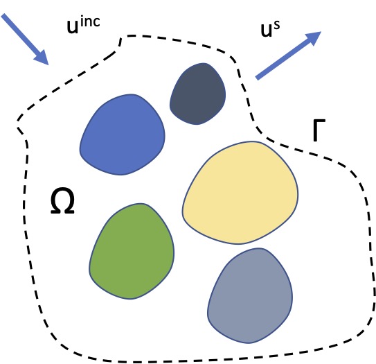
Figure 1: Sketch of the scattering problem under study.

Let us specify a few notations. The unit sphere of $\mathbb{R}^{p}$ is denoted $S^{p-1}$. For $\mathbf{x}\in\mathbb{R}^{p}$, we denote $x=\left|\mathbf{x}\right|,\,\hat{x}=\mathbf{x}/x$ and $k=\omega/c$. We denote $\mathcal{H}_{a}u=\Delta u+k^{2}au$, where the potential $a$ belongs to $L^{\infty}(\mathbb{R}^{p})$. The fundamental solution $g^{+}$ of the Helmholtz equation: $\mathcal{H}_{1}g^{+}=\delta_{0}$ with outgoing wave condition is: $g^{+}(\mathbf{x})=-\frac{1}{4\pi x}e^{ikx}$ for $p=3$ and $g^{+}(\mathbf{x})=-\frac{i}{4}H_{0}^{(1)}(kx)$ for $p=2$. The Green function with the incoming wave condition is denoted $g^{-}(\mathbf{x})$. Explicitly: $g^{-}(\mathbf{x})=-\frac{1}{4\pi x}e^{-ikx}$ for $p=3$, and $g^{-}(\mathbf{x})=-\frac{i}{4}H_{0}^{(2)}(kx)$ for $p=2$. The functions $H_{0}^{(1)}$ and $H_{0}^{(2)}$ are the Hankel functions of first and second type [2].

Let us consider the following time-harmonic scattering problem. Let $\Omega$ be a bounded domain of $\mathbb{R}^{p}$ with boundary $\partial\Omega=\Gamma$, containing a collection of scatterers (see Figure 1). The scatterers are characterized by a potential $a$ such that $a-1$ has a compact support $K\subset\Omega$. For a given incident field $u^{\rm inc}(x)$ satisfying the Helmholtz equation: $\mathcal{H}_{1}u^{\rm inc}=0$, the scattering problem consists in finding the scattered field $u^{s}(\mathbf{x})$ such that the total field $u=u^{\rm inc}+u^{s}$ satisfies:

$$\mathcal{H}_{a}u=0\,,$$

and $u^{s}$ satisfies a radiation condition at infinity: $\partial_{n}u^{s}-iku^{s}=o\left(x^{-1}\right)$ and $u^{s}(\mathbf{x})=O\left(x^{-1}\right)$ when $x\to\infty$.

This scattering problem has a unique solution, as stated in the following lemma:

Lemma 1.

The scattered field $u^{s}$ exists and is unique. There is a linear operator $\mathcal{T}$, the scattering amplitude, relating $u^{\rm inc}$ to $u^{s}$: $u^{s}=\mathcal{T}(u^{\rm inc})$.

Proof.

$\mathcal{H}_{a}(u^{s})=(\mathcal{H}_{1}-\mathcal{H}_{a})(u^{\rm inc})$ and $\mathcal{V}\equiv\mathcal{H}_{1}-\mathcal{H}_{a}$ is null outside the compact region $K$. Then : $\mathcal{H}_{1}(u^{s})=\mathcal{V}(u^{s})+\mathcal{V}(u^{\rm inc})$ and thus: $u^{s}=(1-\mathcal{G}_{1}\mathcal{V})^{-1}\mathcal{G}_{1}\mathcal{V}(u^{\rm inc})$ where the inverse operator $\mathcal{G}_{1}=\mathcal{H}_{1}^{-1}$ is an integral convolution operator with kernel $g^{+}$. ∎

The existence of the resolvent operator is classical although rather subtle (see for instance [3, 4]). This provides a decomposition of the total field in the form:

$$u=u^{\rm inc}+\mathcal{T}(u^{\rm inc}).$$

Let $B_{e}=B(O,R_{e})$ be the smallest ball with center $O$ containing $\Omega$ and $B_{i}=B(O,R_{i})$ the largest ball, with center $O$, contained in $K$. A modal expansion for the scattered field is valid outside $B_{e}$:

$$u^{s}(\mathbf{x})=\left\{\begin{array}[]{l}\sum_{n,m}u^{s}_{nm}h^{(1)}_{n}(kx)Y_{n}^{m}(\hat{x})\hbox{ for }p=3\\ \sum_{n}u^{s}_{n}H^{(1)}_{n}(kx)e^{in\theta}\hbox{ for }p=2\end{array}\right.,\,x>R_{e}.$$ (1)

Here, $h^{(1)}_{n}$ is the spherical Hankel function of first type and order $n$ [2] and $\theta$ is the polar angle of $\mathbf{x}$ in $\mathbb{R}^{2}$.

Whether the functions defined by these series can be extended inside the ball is a difficult problem known as Rayleigh hypothesis, it was essentially solved in the 80’ [8, 9].

Note that, if there is only one scatterer, i.e. $a$ is constant inside $K$, there is also a representation of the field inside $K$ by a series in the following form:

$$u(\mathbf{x})=\left\{\begin{array}[]{l}\sum_{n,m}u^{s}_{nm}j_{n}(kx)Y_{n}^{m}(\hat{x})\hbox{ for }p=3\\ \sum_{n}u^{s}_{n}J_{n}(kx)e^{in\theta}\hbox{ for }p=2\end{array}\right.,\,x<R_{i}.$$ (2)

Here, $J_{n}$ (resp. $j_{n})$ is the Bessel (resp. spherical Bessel) function of order $n$ [2].

When $\overline{\Omega}=K$ and the boundary $\Gamma$ is a sphere, both series can be matched on $\Gamma$, which leads to an explicit form of the scattering coefficients. By considering the traces of the field on the boundary, one can obtain a pseudo-differential operator relating the coefficient of the incident field to that of the scattered field. In the case where $\Gamma$ is not a sphere and $K$ is a proper subset of $\Omega$, this approach can be extended by using an integral representation of the fields: this is the purpose of this work. A pioneering work in that direction can be found in [5].

2 Integral representations of the incident and scattered fields

Our aim is to obtain a representation of the incident and scattered fields as an integral supported by $\Gamma$. Let us first specify some notations.

For $u\in H^{1}(\Omega)$ (the Sobolev space of function of $L^{2}(\Omega)$ with gradient in $L^{2}(\Omega)^{2}$, see [3, chap. 2] for more results on Sobolev spaces), the interior traces [3, chap. 2] of $u$ and its normal derivative on $\Gamma$ are denoted by:

$$\gamma^{-}(u)=\left.u\right|_{\Gamma},\,\gamma^{-}(\partial_{n}u)=\left.\partial_{n}u\right|_{\Gamma}$$ (3)

For fields belonging to $H^{1}_{\rm loc}(\Omega\setminus\mathbb{R}^{p})$, we denote the exterior traces by:

$$\gamma^{+}(u)=\left.u\right|_{\Gamma},\,\gamma^{+}(\partial_{n}u)=\left.\partial_{n}u\right|_{\Gamma}.$$ (4)

Given a field $u\in H^{1}_{\rm loc}(\mathbb{R}^{p})$, we denote $[f]_{\Gamma}$ the jump of $f$ across $\Gamma$, i.e.:

$$[u]_{\Gamma}=\gamma^{+}(u)-\gamma^{-}(u)\hbox{ and }[\partial_{n}u]_{\Gamma}=\gamma^{+}(\partial_{n}u)-\gamma^{-}(\partial_{n}u).$$ (5)

In order to have an integral representation of the fields, we state a result concerning the incident field. To do so, we first need a technical lemma. Note that in the following, the proofs of the results are given for $p=3$ and can be easily adapted for $p=2$ (or, in fact, any other dimension $>1$).

Lemma 2.

Given $\sigma\in H^{-1/2}(\Gamma)$, define:

$$J[\sigma](\hat{x})=\int_{\Gamma}\sigma(\mathbf{x}^{\prime})e^{-ik\hat{x}\cdot\mathbf{x}^{\prime}}d\mathbf{x}^{\prime}.$$ (6)

Assume that $k^{2}$ is not an eigenvalue of $-\Delta$ inside $\Omega$ with Dirichlet boundary conditions on $\Gamma$. If $J[\sigma](\hat{x})=0$, then $\sigma=0$. Moreover $J$ defines a bijection: $H^{-1/2}(\Gamma)\to L^{2}(S^{2})$.

Proof.

Consider the unique function $v$ satisfying $\mathcal{H}_{1}v=0$ in $\Omega\cup(\mathbb{R}^{3}\setminus\overline{\Omega})$ and the boundary conditions:

$$[v]_{\Gamma}=0,\,[\partial_{n}v]_{\Gamma}=\sigma.$$

Then $v$ is represented in the following integral form: $v(\mathbf{x})=\int_{\Gamma}g^{+}(\mathbf{x}-\mathbf{x}^{\prime})\sigma(\mathbf{x}^{\prime})d\mathbf{x}^{\prime}$. Outside $B_{e}$, $v$ can be expanded in spherical harmonics:

$$v(\mathbf{x})=\sum_{mn}v_{nm}h_{n}^{(1)}(kx)Y^{m}_{n}(\hat{x}).$$

The spherical Hankel functions have the following asymptotic forms [2] as $x\to\infty$:

$$h_{n}^{(1)}(kx)\equiv\sqrt{\frac{\pi}{2x}}H^{(1)}_{n+1/2}(x)\sim_{x\to\infty}\frac{e^{i\left(kx-(n+1)\pi/2\right)}}{kx},$$ (7)

$$h_{n}^{(2)}(kx)\equiv\sqrt{\frac{\pi}{2x}}H^{(2)}_{n+1/2}(x)\sim_{x\to\infty}\frac{e^{-i\left(kx-(n+1)\pi/2\right)}}{kx}.$$ (8)

From these relations, we deduce that the following asymptotic behavior holds: ${v(\mathbf{x})\sim\frac{e^{ikx}}{kx}w(\hat{x})}$ with

$$w(\hat{x})=\sum_{nm}v_{nm}e^{-i(n+1)\pi/2}Y_{n}^{m}(\hat{x}).$$

Besides, using the asymptotic form of the Green function:

$$g^{\pm}(\mathbf{x}-\mathbf{x}^{\prime})\sim_{x\to\infty}-\frac{e^{\pm ikx}}{4\pi x}e^{\mp ik\mathbf{x}\cdot\mathbf{x}^{\prime}},$$ (9)

we obtain:

$$v(x)\sim_{x\to\infty}\frac{e^{ikx}}{kx}J[\sigma](\hat{x}),$$

and thus $J[\sigma](\hat{x})=w(\hat{x})$. Consequently, the nullity of $J[\sigma](\hat{x})$ implies that of $w$ and thus that of $v$ in $\mathbb{R}^{3}\setminus\Omega$. Therefore $\gamma_{1}(v)=0$ and $\gamma_{2}(v)$ is non zero iff $v$ is a solution of the Dirichlet problem, therefore $v=0$ everywhere by the hypothesis on $k^{2}$, and thus $\sigma=0$. The surjectivity is obtained as follows. Take a function $\phi\in L^{2}(S^{2})$ and expand it in spherical harmonics:

$$\phi(\hat{x})=\sum_{nm}\phi_{nm}Y_{n}^{m}(\hat{x}).$$

Then construct a field:

$$u(\mathbf{x})=\sum_{nm}\phi_{nm}h_{n}^{(1)}(kx)Y_{n}^{m}(\hat{x}).$$

For a fixed $x>0$, this series converges in $L^{2}(S^{2})$, since $(h_{n}^{(1)}(kx))_{n}$ is a bounded sequence for every $x>0$. Finally, define the field $\tilde{u}$ equals to $u$ outside $\Omega$ and satisfying:

$$\mathcal{H}_{1}\tilde{u}=0\hbox{ in }\Omega,\gamma_{1}(\tilde{u})=\gamma_{1}(u)\hbox{ on }\Gamma.$$

Then $\tilde{u}$ satisfies: $\mathcal{H}_{1}\tilde{u}=[\partial_{n}\tilde{u}]_{\Gamma}\delta_{\Gamma}$ and it holds:

$$\tilde{u}(\mathbf{x})=\int_{\Gamma}[\partial_{n}\tilde{u}]_{\Gamma}g^{+}(\mathbf{x}-\mathbf{x}^{\prime})d\mathbf{x}^{\prime},\,\mathbf{x}\in\mathbb{R}^{3}\setminus\Omega.$$

Therefore, we obtain the existence of $\sigma=[\partial_{n}\tilde{u}]_{\Gamma}\in H^{-1/2}(\Gamma)$. ∎

Using this lemma, we are now in a position to prove the following result that provides a representation of the incident field as an integral over $\Gamma$:

Theorem 1.

The incident field can be represented in the form:

$$u^{\rm inc}(\mathbf{x})=i\int_{\Gamma}\sigma^{\rm inc}(\mathbf{x}^{\prime})\Im(g^{+}(\mathbf{x}-\mathbf{x}^{\prime}))dr^{\prime},\,\mathbf{x}\in\mathbb{R}^{p}$$

where $\sigma^{\rm inc}$ belongs to $H^{-1/2}(\Gamma)$.

Proof.

The incident field can be expanded in spherical harmonics in the form ${u^{\rm inc}=u^{+}+u^{-}}$, where:

$$u^{+}(\mathbf{x})=\frac{1}{2}\sum_{nm}i_{nm}h_{n}^{(1)}(kx)Y_{n}^{m}(\hat{x}),\,u^{-}(\mathbf{x})=\frac{1}{2}\sum_{nm}i_{nm}h_{n}^{(2)}(kx)Y_{n}^{m}(\hat{x}).$$

Using the asymptotic forms of the spherical Hankel functions (7,8) we obtain the existence of two functions $u^{\pm}_{\infty}(\hat{x})$ defined on $S^{2}$ and such that:

$$u^{\rm inc}(x)\sim\frac{e^{ikx}}{kx}u^{+}_{\infty}(\hat{x})+\frac{e^{-ikx}}{kx}u^{-}_{\infty}(\hat{x})$$

Explicitly, these functions are given by:

$$u^{+}_{\infty}(\hat{x})=\frac{1}{2}\sum_{nm}i_{nm}e^{-i(n+1)\pi/2}Y_{n}^{m}(\hat{x}),\,u^{-}_{\infty}(\hat{x})=\frac{1}{2}\sum_{nm}i_{nm}e^{i(n+1)\pi/2}Y_{n}^{m}(\hat{x}).$$

Since:

$$e^{-i(n+1)\pi/2}=(-1)^{n+1}e^{i(n+1)\pi/2}\hbox{ and }Y_{n}^{m}(-\hat{x})=(-1)^{n}Y_{n}^{m}(\hat{x}),$$

we have that:

$$u^{-}_{\infty}(-\hat{x})=\frac{1}{2}\sum_{nm}i_{nm}e^{i(n+1)\pi/2}Y_{n}^{m}(-\hat{x})=\frac{1}{2}\sum_{nm}i_{nm}(-1)^{n}e^{i(n+1)\pi/2}Y_{n}^{m}(\hat{x})$$

$$=-\frac{1}{2}\sum_{nm}i_{nm}e^{-i(n+1)\pi/2}Y_{n}^{m}(\hat{x})=-u^{+}_{\infty}(\hat{x}).$$

Consider now the field $\tilde{u}^{\rm inc}$, defined by the following integral:

$$\tilde{u}^{\rm inc}(\mathbf{x})=\frac{1}{2}\int_{\Gamma}\left[\sigma^{\rm inc}(\mathbf{x}^{\prime})g^{+}(\mathbf{x}-\mathbf{x}^{\prime})-\sigma^{\rm inc}(\mathbf{x}^{\prime})g^{-}(\mathbf{x}-\mathbf{x}^{\prime})\right]d\mathbf{x}^{\prime}.$$

Due to the continuity properties of a single layer potential [6], it satisfies $\mathcal{H}_{1}\tilde{u}^{\rm inc}=0$ . Using (9), it is given asymptotically as $x\to\infty$, by:

$$\tilde{u}^{\rm inc}(\mathbf{x})\sim\frac{e^{ikx}}{kx}\int_{\Gamma}\sigma^{\rm inc}(\mathbf{x}^{\prime})e^{-ik\hat{x}\cdot\mathbf{x}^{\prime}}d\mathbf{x}^{\prime}-\frac{e^{-ikx}}{kx}\int_{\Gamma}\sigma^{\rm inc}(\mathbf{x}^{\prime})e^{ik\hat{x}\cdot\mathbf{x}^{\prime}}d\mathbf{x}^{\prime}$$

Therefore, the existence of $\sigma^{\rm inc}$ satisfying: $u^{+}_{\infty}(\hat{x})=\int_{\Gamma}\sigma^{\rm inc}(\mathbf{x}^{\prime})e^{-ik\hat{x}\cdot\mathbf{x}^{\prime}}d\mathbf{x}^{\prime}$ follows from lemma (2) and the second relation:

$$u^{-}_{\infty}(\hat{x})=-\frac{e^{-ikx}}{kx}\int_{\Gamma}\sigma^{\rm inc}(\mathbf{x}^{\prime})e^{ik\hat{x}\cdot\mathbf{x}^{\prime}}d\mathbf{x}^{\prime}$$

is fulfilled thanks to:

$$u^{-}_{\infty}(\hat{x})=-u^{+}_{\infty}(-\hat{x})=-\int_{\Gamma}\sigma^{\rm inc}(\mathbf{x}^{\prime})e^{ik\hat{x}\cdot\mathbf{x}^{\prime}}d\mathbf{x}^{\prime}.$$

We conclude from Rellich lemma [3, p. 74] that $u^{\rm inc}=\tilde{u}^{\rm inc}$, since both fields satisfy the same equation and the same asymptotic behavior at infinity. The integral expression follows by noting that $g^{+}$ and $g^{-}$ are complex conjugated functions.

∎

Our next result is that the scattered field can also be represented by an integral over $\Gamma$:

Theorem 2.

There exists $\sigma^{s}\in H^{-1/2}(\Gamma)$ such that:

$$u^{s}(\mathbf{x})=\int_{\Gamma}\sigma^{s}(\mathbf{x}^{\prime})g^{+}(\mathbf{x}-\mathbf{x}^{\prime})d\mathbf{x}^{\prime},\mathbf{x}\in\mathbb{R}^{p}\setminus\Omega.$$ (10)

Proof.

Consider the field $\tilde{u}^{s}$ that is equal to $u^{s}$ outside $\Omega$ and that satisfies the following problem inside $\Omega$:

$$\mathcal{H}_{1}\tilde{u}^{s}=0\hbox{ inside }\Omega,\,\left.\tilde{u}^{s}\right|_{\Gamma}=\left.u^{s}\right|_{\Gamma}.$$

Over $\mathbb{R}^{p}$, it satisfies: $\mathcal{H}_{1}\tilde{u}^{s}=[\partial_{n}\tilde{u}^{s}]_{\Gamma}\delta_{\Gamma}.$ Given the outgoing wave condition at infinity, this gives:

$$u^{s}(\mathbf{x})=\int_{\Gamma}[\partial_{n}\tilde{u}^{s}]_{\Gamma}g^{+}(\mathbf{x}-\mathbf{x}^{\prime})d\mathbf{x}^{\prime},$$

and consequently the existence of the density $\sigma^{s}=[\partial_{n}\tilde{u}^{s}]_{\Gamma}$ belonging to $H^{-1/2}(\Gamma)$. ∎

We can now deduce the following representation result for the total field:

Corollary 1.

The total field $u$ can be written in the form

$$u(\mathbf{x})=u^{\rm tot,+}(\mathbf{x})+u^{\rm tot,-}(\mathbf{x}),$$ (11)

where

$$u^{\rm tot,+}(\mathbf{x})=\int_{\Gamma}\sigma^{+}(\mathbf{x}^{\prime})g^{+}(\mathbf{x}-\mathbf{x}^{\prime})d\mathbf{x}^{\prime},\,u^{\rm tot,-}(\mathbf{x})=\int_{\Gamma}\sigma^{-}(\mathbf{x}^{\prime})g^{-}(\mathbf{x}-\mathbf{x}^{\prime})dx^{\prime},$$ (12)

and $\sigma^{+},\sigma^{-}$ belong to $H^{-1/2}(\Gamma)$.

Proof.

This is a direct consequence of theorem 1 and theorem 2. Putting the scattered field and the incident field together, we obtain:

$$\sigma^{+}=[\partial_{n}\tilde{u}^{s}]_{\Gamma}+\frac{1}{2}\sigma^{\rm inc},\,\sigma^{-}=-\frac{1}{2}\sigma^{\rm inc}.$$ (13)

∎

3 Discussion and a numerical example

3.1 A numerical example

Let us consider the scattering of an electromagnetic plane wave in $E_{||}$ polarization by a collection of cylinders contained in a domain whose cross section $\Omega$ is bounded by an astroid $\Gamma$ (cf. Figure 2).

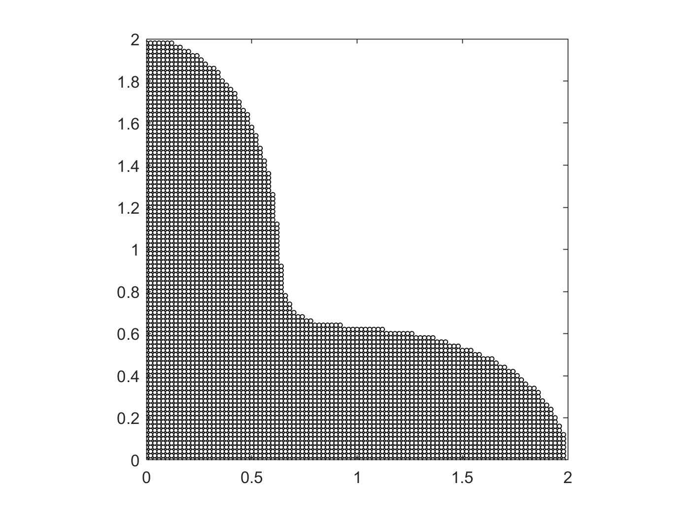
Figure 2: One quarter of the domain $\Omega$: it is a smooth astroid filled with small dielectic rods.

For numerical purpose, the units are that defined by the wavelength and we choose $\lambda=1$. The astroid contains $N=4657$ rods with relative permittivity 12. We use the multiple scattering approach described in [7].

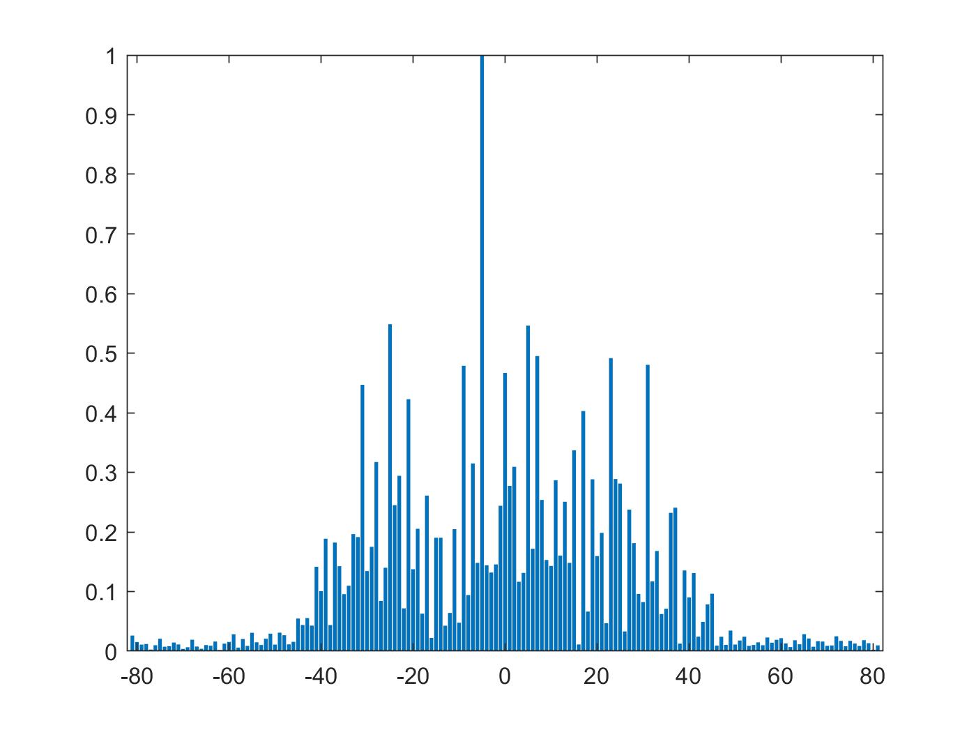
Figure 3: Normalized Discrete Fourier Transform coefficients of the sequence of coefficients $(s_{k})$.

We assume that the rods, at positions $(\mathbf{x}_{k})$, are small enough that they can each be characterized by only one scattering coefficient $s^{0}_{q}$ [7]. We denote $\mathbf{x}=(x_{1},x_{2})$.

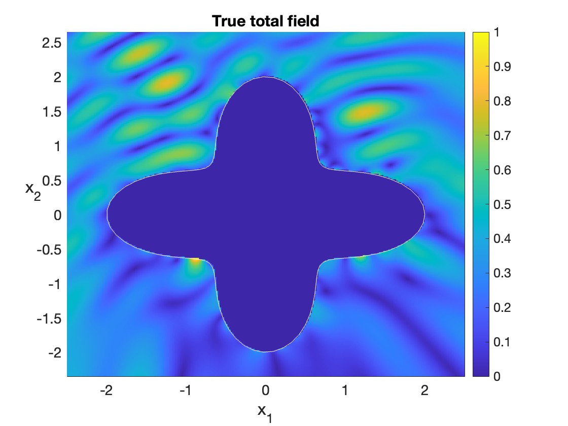
Figure 4: Map of the normalized modulus of the total field outside the astroid, computed by a direct summation over all the scatteres contained inside $\Omega$.

Figure 5: Map of the normalized modulus of the total field outside the astroid, computed by using the single layer representation of the scattered field.

At this step the scattered field is represented, everywhere outside the cylinders, by a sum over the rods in the form:

$$u^{s}(\mathbf{x})=\sum_{q=1}^{N}s^{0}_{q}H^{(1)}_{0}(k|\mathbf{x}-\mathbf{x}_{q}|).$$ (14)

The coefficients $\hat{s}=(s^{0}_{q})_{1,\ldots,N}$ are determined from the multiple scattering theory [7]. The scattering coefficient $s^{0}_{q}$ is related to the local incident field $u^{\rm inc,loc}_{q}$ through the scattering amplitude $t^{0}_{q}$: $s^{0}_{q}=t^{0}_{q}u^{\rm inc,loc}_{q}$. For a circular dielectric rod of radius $r_{q}$ and relative permittivity $\varepsilon_{q}=\nu_{q}^{2}$, it holds:

$$t^{0}_{q}=-\frac{J_{1}(kr_{q})J_{0}(k\nu_{q}r_{q})-\nu_{q}J_{0}(kr_{q})J_{1}(k\nu_{q}r_{q})}{H^{(1)}_{1}(kr_{q})J_{0}(k\nu_{q}r_{q})-\nu_{q}H^{(1)}_{0}(kr_{q})J_{1}(k\nu_{q}r_{q})}.$$

The local incident field is:

$$u^{\rm inc,loc}_{q}=u^{\rm inc}(\mathbf{x}_{q})+\sum_{j\neq q}s^{0}_{j}H_{0}^{(1)}(|\mathbf{x}_{q}-\mathbf{x}_{j}|).$$ (15)

Therefore, it holds:

$$s^{0}_{q}=t^{0}_{q}\left(u^{\rm inc}(\mathbf{x}_{q})+\sum_{j\neq q}s^{0}_{j}H_{0}^{(1)}(|\mathbf{x}_{q}-\mathbf{x}_{j}|)\right).$$ (16)

Let us denote $\overline{\overline{t}}$ the diagonal matrix defined by $\overline{\overline{t}}=diag(t^{0}_{1},\ldots,t^{0}_{N})$ and $\overline{\overline{h}}$ the matrix with entries $h_{ij}=H_{0}^{(1)}(|\mathbf{x}_{i}-\mathbf{x}_{j}|)$ for $i\neq j$ and $h_{ii}=0$. The coefficients $\hat{s}$ are obtained by solving the system:

$$\left((\overline{\overline{t}})^{-1}-\overline{\overline{h}}\right)\hat{s}=\hat{u}^{\rm inc}$$ (17)

where $\hat{u}^{\rm inc}=(u^{\rm inc}(\mathbf{x}_{q}))_{1,\ldots,N}$.

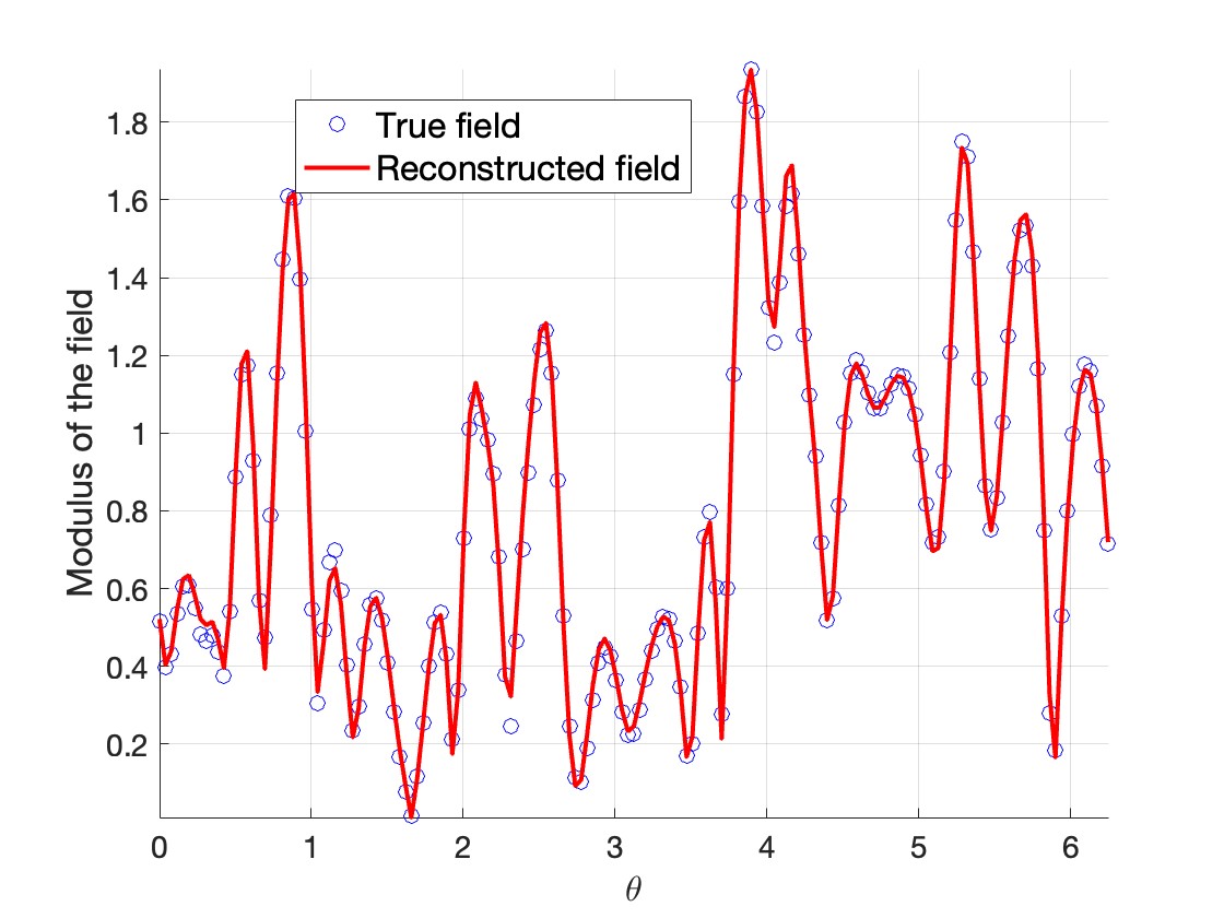
Figure 6: Modulus of the total field on a curve deduced from $\Gamma$ by a homothety of ratio 1.3. The red curve corresponds to the total field reconstructed by means of the single layer representation and the blue circles correspond to the total field computed by a direct summation over all the scatterers.

The point is to be able to represent the scattered field by means of a single layer potential as explained in section (2). The unicity of $\sigma^{s}$ being ensured by theorem (1), it can be determined by solving an integral equation of the first kind by imposing

$$\int_{\Gamma}\sigma^{s}(\mathbf{x}^{\prime})H^{(1)}_{0}(\mathbf{x}-\mathbf{x}^{\prime})d\mathbf{x}^{\prime}=u^{s}(\mathbf{x}),\mathbf{x}\in\Gamma.$$

In order to do so numerically, that is, to obtain a discretized version of the density $\sigma^{s}$, we simply write a discrete version of the integral:

$$u^{s}_{P}(\mathbf{x})=\sum_{p=1}^{P}\sigma^{s}_{p}H^{(1)}_{0}(k|\mathbf{x}-\mathbf{y}_{p}|),$$ (18)

and the points $(\mathbf{y}_{p})$ are put uniformly on $\Gamma$. On $\Gamma$, the scattered field can be written:

$$u^{s}_{p}\equiv u^{s}(\mathbf{y}^{\prime}_{p})=\sum_{q=1}^{N}s^{0}_{q}H^{(1)}_{0}(k|\mathbf{y}^{\prime}_{p}-\mathbf{x}_{q}|),\,\mathbf{y}^{\prime}_{p}\in\Gamma,p=1,\ldots,P.$$

The second set of points $(\mathbf{y}^{\prime}_{p})$ is different from $(\mathbf{y}_{p})$ in order to avoid the $0$ singularity of the Hankel function. In matrix form, this reads as:

$$\overline{\overline{H}}\hat{s}=\hat{u}^{s}$$ (19)

where $\hat{u}^{s}=(u^{s}_{p})$. Let us remark that $\overline{\overline{H}}$ is a $P\times N$ matrix. Then a square linear system is obtained by writing:

$$\sum_{p=1}^{P}\sigma^{s}_{p}H^{(1)}_{0}(k|\mathbf{y}^{\prime}_{p^{\prime}}-\mathbf{y}_{p}|)=u^{s}_{p^{\prime}},\,p^{\prime}=1\ldots P.$$

In matrix form, this can be written:

$$\overline{\overline{I}}\hat{\sigma}^{s}=\hat{u}^{s},$$ (20)

where: $\hat{\sigma}^{s}=(\sigma^{s}_{p})$ and $\overline{\overline{I}}$ is a $P\times P$ matrix with entries $I_{pp^{\prime}}=H^{(1)}_{0}(k|\mathbf{y}^{\prime}_{p^{\prime}}-\mathbf{y}_{p}|)$. Finally, we obtain a matrix $\overline{\overline{B}}$ relating $\hat{s}^{s}$ to $\hat{\sigma}^{s}$:

$$\overline{\overline{B}}=(\overline{\overline{I}})^{-1}\overline{\overline{H}}.$$ (21)

This matrix is a $P\times N$ matrix.

Heuristically, the number $P$ can be determined by recalling that the function $\sigma^{s}$ is periodic, since it is defined on a bounded curve. Consequently, the computation of the DFT of $(\sigma^{s}_{p})_{p\in\{1,\ldots P\}}$ can indicate whether the approximation is good, by checking the decreasing of the Fourier coefficients. This is examplified in Figure 3 where we have computed the DFT of the finite sequence $(\sigma^{s}_{p})$. It is important to have this criterium, since the discrete values of the density $(\sigma^{s}_{p})$ do not have a decreasing behavior with $P$. The final value is $P=160$.

We are able to reconstruct with a very good precision the diffracted field. In Figure 4 we have plotted a map of the total field outside the region where the scatterers are contained, obtained by summing the contributions of the dielectric rods, and in Figure 5 it is the reconstructed field. Both fields have been normalized so that their maximal value is equal to 1, in order to have the same color scale. For a more direct comparison, in Figure 6 we have plotted the total field on a curve deduced from $\Gamma$ by a homothety of ratio 1.3. We stress that, thanks to this approach the representation of the scattered field is now ensured by $160$ terms instead of 4657.

3.2 Extension of the Fast Multipole Method

It is important to remark that the single layer representation involves a surface $\Gamma$, enclosing the scatterers, that can be chosen at will. By this we mean that, given a set of scatterers and any smooth enough surface $\Gamma$ enclosing this set, the field scattered by this set and the incident field can be represented by an integral over $\Gamma$. This result is in fact a generalization of the expansion over spherical harmonics and spherical Bessel functions to an arbitrary surface. As a consequence, it is possible to split a given set of scatterers into several subset, apply multiple scattering theory to each smaller subset then use the representation by the single layers to couple the subsets in between them. In order to do so, an iterative algorithm is to be used. Let us be more specific: we put $p=2$ and consider simply two subsets $O^{1}=\cup_{j=1}^{N^{1}}\Omega^{1}_{j}$ and $O^{2}=\cup_{j=1}^{N^{2}}\Omega^{2}_{j}$ and two surfaces $\Gamma_{1}$ and $\Gamma_{2}$ enclosing respectively $O^{1}$ and $O^{2}$ (see Figure 7).

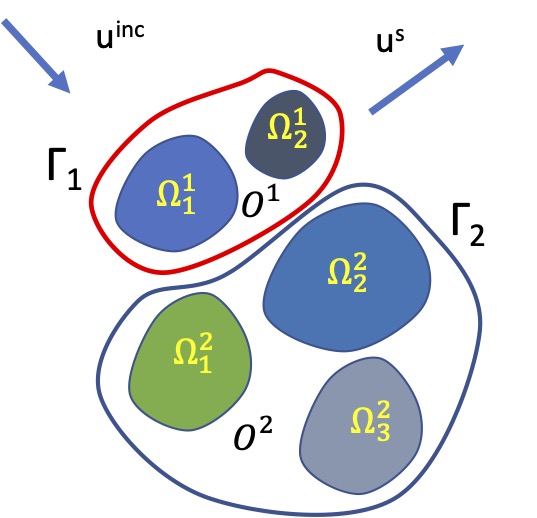
Figure 7: Sketch of the scattering problem with two subsets.

The incident field $u^{\rm inc}$ illuminates $O^{1}$ and $O^{2}$. As in the preceding section, we assume for simplicity that the wavelength is large enough that the obstacle $\Omega^{\alpha}_{j}$ ($\alpha=1,2$) can be considered to be a point at coordinate $\mathbf{x}_{j}^{\alpha}$, and that the field scattered by $\Omega^{\alpha}_{j}$ reads as:

$$u^{s,\alpha}_{j}(\mathbf{x})=s^{0,\alpha}_{j}H_{0}^{(1)}(k|\mathbf{x}-\mathbf{x}^{\alpha}_{j}|)$$

For each scatterer $\Omega^{1}_{j}\in O^{1}$, the incident field is the sum of the ”true” incident field $u^{\rm inc}(\mathbf{x}^{1}_{j})$ and the field coming from the other subset $O^{2}$ and given by the discrete single layer representation:

$$u^{s,2}(\mathbf{x}^{1}_{j})=\sum_{p=1}^{P_{2}}\sigma_{p}^{s,2}(\mathbf{y}_{p})H_{0}^{(1)}(k|\mathbf{x}^{1}_{j}-\mathbf{y}_{p}|).$$ (22)

Of course, there is the same set of relations obtained by making the switching $1\leftrightarrow 2$. Here the local incident field is therefore:

$$u^{\rm inc,loc}_{j}=u^{\rm inc}(\mathbf{x}^{1}_{j})+u^{s,2}(\mathbf{x}^{1}_{j}).$$ (23)

We denote the diagonal matrix $\overline{\overline{t^{\alpha}}}=diag(t^{0,\alpha}_{1},\ldots,t^{0,\alpha}_{N_{\alpha}})$, $\hat{u}^{s,2}=(u^{s,2}(x^{1}_{j}))$ (resp. $\hat{u}^{s,1}=(u^{s,1}(\mathbf{x}^{2}_{j}))$) and $\hat{u}^{{\rm inc},{\alpha}}=(u^{\rm inc}(\mathbf{x}^{\alpha}_{j}))$. As in the preceding section, the operator that relates the scattering coefficients $\hat{s}^{\alpha}=(s^{0,\alpha}_{j})$ to the discretized density $\hat{\sigma}^{s,\alpha}=(\sigma^{s,\alpha}_{p})$ is denoted by $\overline{\overline{B}}^{\alpha}$ (cf. (21)):

$$\hat{\sigma}^{\alpha}=\overline{\overline{B}}^{\alpha}\,\hat{s}^{\alpha}.$$ (24)

It is a $P_{\alpha}\times N_{\alpha}$ matrix. Finally, $\overline{\overline{R}}^{\alpha}$ is the matrix that relates $\hat{\sigma}^{s,\alpha}$ to $\hat{u}^{s,\alpha}$:

$$\hat{u}^{s,\alpha}=\overline{\overline{R}}^{\alpha}\,\hat{\sigma}^{\alpha}.$$ (25)

Explicitly (taking $\alpha=2$):

$$\hat{u}^{s,2}(\mathbf{x}^{1}_{j})=\sum_{p=1}^{P_{2}}H_{0}^{(1)}(|\mathbf{x}^{1}_{j}-\mathbf{y}^{2}_{p}|)\,\sigma^{s,2}_{p},\,j=1,\ldots N_{1}.$$ (26)

Therefore $\overline{\overline{R}}^{2}$ as entries: $R^{2}_{ij}=H_{0}^{(1)}(|\mathbf{x}^{1}_{i}-\mathbf{y}^{2}_{j}|),\,i=1,\ldots N_{1},\,j=1,\ldots P_{2}$. It is a $N_{1}\times P_{2}$ matrix. Finally, the linear system to be solved is:

$$\left[\begin{pmatrix}(\overline{\overline{t^{1}}})^{-1}&0\\ 0&(\overline{\overline{t^{2}}})^{-2}\end{pmatrix}-\begin{pmatrix}\overline{\overline{h}}^{1}&\overline{\overline{R}}^{2}\overline{\overline{B}}^{2}\\ \overline{\overline{R}}^{1}\overline{\overline{B}}^{1}&\overline{\overline{h}}^{2}\end{pmatrix}\right]\begin{pmatrix}\hat{s}^{1}\\ \hat{s}^{2}\end{pmatrix}=\begin{pmatrix}\hat{u}^{\rm inc,1}\\ \hat{u}^{\rm inc,2}\end{pmatrix}.$$ (27)

The numerical gain here lies in the diagonal terms $\overline{\overline{R}}^{\alpha}\overline{\overline{B}}^{\alpha}$. If we were to use directly the multiple scattering theory, we would have to compute these terms by coupling directly each cylinder to every other cylinder, which would involve the direct computation of the matrix with entries $H_{0}^{(1)}(|\mathbf{x}^{1}_{i}-\mathbf{x}^{2}_{j}|)$ of size $N_{1}\times N_{2}$. Here, we have to compute directly the matrix $\overline{\overline{h}}^{1}$ (resp. $\overline{\overline{h}}^{2}$) of size $N_{1}\times N_{1}$ (resp. $N_{2}\times N_{2}$) and then the coupling between the two subsets is ensured by the terms $\overline{\overline{R}}^{1}\overline{\overline{B}}^{1}$ and $\overline{\overline{R}}^{2}\overline{\overline{B}}^{2}$. While these matrices are of course of size $N_{2}\times N_{1}$ (resp. $N_{1}\times N_{2}$) they are obtained as the product of matrices of size $N_{2}\times P_{1}$ and $P_{1}\times N_{1}$ (resp. $N_{1}\times P_{2}$ and $P_{2}\times N_{1}$ ).

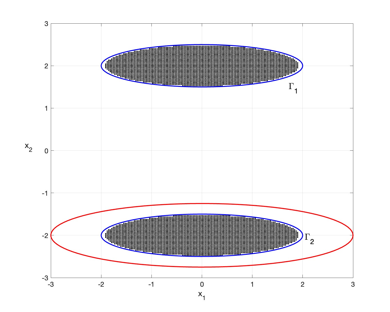
Figure 8: Two elliptic subsets containing each $3234$ dielectric cylinders. The red ellipsis indicates where the field is computed in Figure 10.

Let us give a numerical example. We consider two subsets of dielectric rods contained in two elliptical domains, as depicted in Figure 8. The incident field is a plane wave $u^{\rm inc}(\mathbf{x})=e^{-ikx_{2}}$ . As in the first numerical example, the length unit is that of the wavelength and we choose $\lambda=10$. There are $3234$ rods with radius $0.015$ and relative permittivity $\varepsilon=10$ in each domain. The map of the field is given in Figure 9. We have computed the maps by using the single layer representation (left panel) and by using the multiple scattering theory for the entire set of rods in the right panel. We have used $P_{1}=P_{2}=100$ points to compute the single layer representations (22). The maps and the scattering coefficients agree to a precision below $0.3\%$ (in $L^{2}$ norm for the entire region covered by the map).

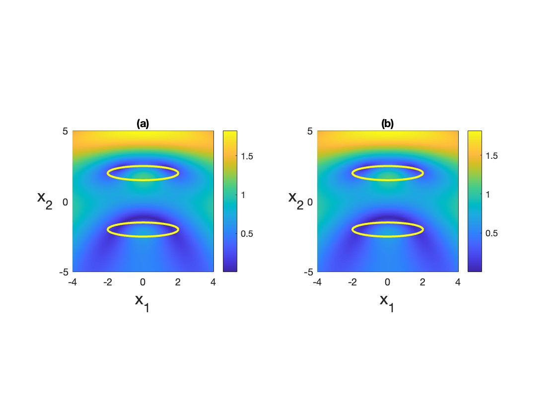
Figure 9: Maps of the modulus field. On the left (a) panel, the field is computed by using the extended Fast Multipole Method, on the right (b) panel, it is computed by using directly the multiple scattering theory for the entire set of cylinders.

In Figure 10, we have plotted the modulus of the scattered field on the red ellipsis plotted in Figure 8. The fields coincide to $0.6\%$.

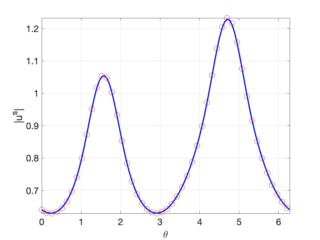
Figure 10: The curve in solid line corresponds to the field computed by using directly the single layer representations of the fields scattered by each subset (cf. (18)). The circles corresponds to the field computed by summing over the contribution of each cylinder (cf. (14)).

The calculation time on a laptop for the single layer approach is around $2$ to $3$ times faster than for the direct multiple scattering approach. It is to be noted that the number of points $P_{1,2}$ plays a negligible role in the total calculation time: reducing $P_{1}=P_{2}$ to $30$ does not change the calculation time up to the time fluctuations.

In conclusion, we have established a new way of representing the field scattered by a large collection of object by using a single layer representation. The scattered field is characterized by a density supported by the boundary of a domain containing the scatterers. From a numerical point of view, the gain lies in the number of parameters needed to represent the field. Since the sources are supported by a region of codimension 1, much less information is needed, as compared to a volumetric representation (of codimension 0). This result in a drastic reduction of the number of values required for representing the scattered field with a given precision. This result is a generalization of the representation of the field by spherical harmonics used in the Fast Multiple Method and extend this algorithm beyond the spherical geometry.

References

References

- [1] Gumerov N and Duraiswami R 2004 Fast Multipole Methods for the Helmholtz Equation in Three Dimensions (Elsevier: Amsterdam).
- [2] Abramowitz M and Stegun I 1964 Handbook of Mathematical Functions (Dover: London).
- [3] Cessenat M 1996 Mathematical Methods in Electromagnetism(World Scientific: Singapore).
- [4] Melrose R 1995 Geometric scattering theory (Cambridge University Press: Cambridge).
- [5] Maystre D 2006 Electromagnetic scattering by a set of objects: an integral methods based on scattering properties PIER 57 55-84.
- [6] Colton D and Kress R 2013 Integral Equation Method in Scattering Theory (SIAM: Philadelphia).
- [7] Felbacq D, Tayeb G and Maystre D 1995 Scattering by a random set of parallel cylinders J. Opt. Soc. Am. A 11 2526-2538.
- [8] Millar R F 1980 The Analytic Continuation of Solutions to Elliptic Boundary Value Problems in Two Independent Variables J. Math. Anal. Appl. 76 498-515.
- [9] Maystre D and Cadilhac M 1985 Singularities of the continuation of fields and validity of Rayleigh’s hypothesis J. Math. Phys. 26 2201-2204.