PROXIMAL BELLMAN MAPPINGS FOR REINFORCEMENT LEARNING
AND THEIR APPLICATION TO ROBUST ADAPTIVE FILTERING

Abstract

This paper aims at the algorithmic/theoretical core of reinforcement learning (RL) by introducing the novel class of proximal Bellman mappings. These mappings are defined in reproducing kernel Hilbert spaces (RKHSs), to benefit from the rich approximation properties and inner product of RKHSs, they are shown to belong to the powerful Hilbertian family of (firmly) nonexpansive mappings, regardless of the values of their discount factors, and possess ample degrees of design freedom to even reproduce attributes of the classical Bellman mappings and to pave the way for novel RL designs. An approximate policy-iteration scheme is built on the proposed class of mappings to solve the problem of selecting online, at every time instance, the “optimal” exponent $p$ in a $p$-norm loss to combat outliers in linear adaptive filtering, without training data and any knowledge on the statistical properties of the outliers. Numerical tests on synthetic data showcase the superior performance of the proposed framework over several non-RL and kernel-based RL schemes.

1 Introduction

In reinforcement learning (RL) [1], an agent takes a decision/action based on feedback provided by the surrounding environment on the agent’s past actions. RL is a sequential-decision-making framework with the goal of minimizing the long-term loss/price $Q$ to be paid by the agent for its own decisions. RL has deep roots in dynamic programming [1, 2], and a far-reaching range of applications which extend from autonomous navigation, robotics, resource planning, sensor networks, biomedical imaging, and can reach even to gaming [1].

This paper aims at the algorithmic/theoretical core of RL by introducing the novel class of proximal Bellman mappings (3), defined in reproducing kernel Hilbert spaces (RKHSs), which serve as approximating spaces for the one-step $g$ and long-term $Q$ losses in RL, and are well known for their rich properties, such as the reproducing property of their inner product [3, 4]. This study stands as the first stepping stone for (i) a simple, flexible and general framework, which can even reproduce attributes of the classical Bellman mappings (2), such as their fixed-point sets or the mappings themselves (see Proposition 1), and for (ii) the exciting combination of arguments from RKHSs and nonparametric-approximation theory [5] with the powerful Hilbertian toolbox of nonexpansive mappings [6]; see Theorem 1.

Usually in RL, $g$ and $Q$ are considered as points of the Banach space $\mathcal{B}$ of all (essentially) bounded functions [7], equipped with the $\mathcal{L}_{\infty}$-norm. As such, Bellman mappings operate from $\mathcal{B}$ to $\mathcal{B}$, they are shown to be contractions [6] by appropriately constraining the values of their discount factors (see (2)), and possess thus unique fixed points [6]. Unfortunately, $\mathcal{B}$ lacks an inner product by definition. To overcome this inconvenience, the popular strategy in RL is to assume that $g,Q$ are spanned by a basis of vectors, usually learned from training data, with a fixed and finite cardinality, which amounts to saying that $g,Q$ belong to a Euclidean vector space of fixed dimension. These modeling assumptions can be met in almost all currently popular RL frameworks, from temporal difference (TD) [1] and least-squares (LS)TD [8, 9, 10], to Bellman-residual (BR) methodologies [11] and kernel-based RL (KBRL) [12, 13, 14, 15, 16, 11, 9, 17]. Notwithstanding, the Bellman mappings introduced in [12, 13] are still defined on Banach spaces, with no guarantees that they operate from an RKHS $\mathcal{H}$ to $\mathcal{H}$. Although [18, 19] utilize RKHSs, they do not discuss Bellman mappings. Proximal mappings have been used in [20] only in the popular context of minimizing loss functions, without any consideration of using proximal mappings directly as Bellman ones.

Unlike typical contraction-based designs in Banach spaces, the novel proximal Bellman mappings (3) are shown to be (firmly) nonexpansive with potentially non-unique fixed points in RKHSs, regardless of the value of their discount factors (see Theorem 1). This result improves upon the result of the predecessor [21] of this work, where the nonexpansivity of the introduced Bellman mappings was established via appropriate conditions on their discount factors. Moreover, the benefit of using potentially infinite-dimensional RKHSs comes also from the freedom of allowing for $Q$-function representations by dynamically changing bases, with variable and even growing cardinality, to accommodate online-learning scenarios where the basis vectors are not learned solely from (offline) training data, but may be continuously and dynamically learned also from streaming (online) test data.

To highlight such online-learning settings, this study considers robust adaptive filtering [22] as the application domain of the proximal Bellman mappings (3). The goal is to combat outliers in the classical data-generation model $y_{n}=\boldsymbol{\theta}_{*}^{\intercal}\mathbf{x}_{n}+o_{n}$, where $n\in\mathbb{N}$ denotes discrete time ($\mathbb{N}$ is the set of all non-negative integers), $\boldsymbol{\theta}_{*}$ is the $L\times 1$ vector whose entries are the system parameters that need to be identified, $(\mathbf{x}_{n},y_{n})$ stands for the input-output pair of available data, where $\mathbf{x}_{n}$ is an $L\times 1$ vector and $y_{n}$ is real-valued, and $\intercal$ denotes vector/matrix transposition. Outliers $o_{n}$ are defined as contaminating data that do not adhere to a nominal data generation model [23], and are often modeled as random variables (RVs) with non-Gaussian heavy tailed distributions, e.g., $\alpha$-stable ones [24].

Since the least-squares (LS) error criterion is notoriously sensitive to outliers [23], non-LS criteria, such as least mean p-power (LMP) [25, 26, 27, 28, 29, 30, 31] and maximum correntropy (MC) [32], have been studied instead of LS ones in robust adaptive filtering. To avoid a lengthy exposition, this work focuses on the LMP criterion and algorithm [25], which, for an arbitrarily fixed $\boldsymbol{\theta}_{0}$, generates estimates $(\boldsymbol{\theta}_{n})_{n\in\mathbb{N}}$ of $\boldsymbol{\theta}_{*}$ as follows:

$$\boldsymbol{\theta}_{n+1}\coloneqq\boldsymbol{\theta}_{n}+\rho p\lvert e_{n}\rvert^{p-2}e_{n}\mathbf{x}_{n}\,,$$ (1)

where $e_{n}\coloneqq y_{n}-\mathbf{x}_{n}^{\intercal}\boldsymbol{\theta}_{n}$, $\rho$ is the learning rate (step size), and $p$ is a fixed user-defined real-valued number within the interval $[1,2]$ to ensure that the $p$-norm loss $\lvert y_{n}-\mathbf{x}_{n}^{\intercal}\boldsymbol{\theta}\rvert^{p}$ is a convex function of $\boldsymbol{\theta}$ [25]. Notice that if $p=1$ and $2$, then (1) boils down to the classical sign-LMS and LMS, respectively [22]. Combination of adaptive filters with different forgetting factors but with the same fixed $p$-norm [29], as well as with different $p$-norms [33] have been also considered.

This paper provides an online and data-driven solution to the problem of dynamically selecting $p$ by using the proposed proximal Bellman mappings, without any prior knowledge on the statistical properties of $o_{n}$. It is worth mentioning that this work and its predecessor [21] are the first attempts in the literature to apply RL arguments to robust adaptive filtering. Algorithm 1 offers an approximate policy-iteration (API) strategy, where the underlying state space is considered to be the low-dimensional $\mathbb{R}^{4}$, independent of the dimension $L$ of $\boldsymbol{\theta}_{*}$, whereas [21] uses the high-dimensional $\mathbb{R}^{2L+1}$. The action space is considered to be discrete: an action is a value of $p$ taken from a finite grid of the interval $[1,2]$. Moreover, experience replay [34] (past-data reuse) is introduced, unlike the classical Bellman operators where information on transition probabilities in a Markov decision process is required in advance [1]. Note that [21] employs rollout for data reuse and exploration [1].

Numerical tests on synthetic data showcase the superior performance of the advocated framework over several non-RL and RL schemes. Due to space limitations, proofs, the convergence analysis of the proposed algorithm, as well as further RL designs and numerical tests will be reported elsewhere.

2 Proximal Bellman Mappings

First, some key RL concepts are in order [1]. The state space is denoted in general by $\mathfrak{S}\subset\mathbb{R}^{D}$, with a state vector $\mathbf{s}\in\mathfrak{S}$, and the action space by $\mathfrak{A}$, with action $a\in\mathfrak{A}$. For convenience, the state-action tuple is defined as $\mathbf{z}\coloneqq(\mathbf{s},a)\in\mathfrak{Z}\coloneqq\mathfrak{S}\times\mathfrak{A}$. The classical Bellman mappings, e.g., [35]: $\forall(\mathbf{s},a)\in\mathfrak{Z}$,

$$(T_{\mu}^{\diamond}Q)(\mathbf{s},a) \coloneqq g(\mathbf{s},a)+\alpha\mathbb{E}_{\mathbf{s}^{\prime}{\mathbin{}\mid\mathbin{}}(\mathbf{s},a)}\{Q(\mathbf{s}^{\prime},\mu(\mathbf{s}^{\prime}))\}\,,$$ (2a)

$$(T^{\diamond}Q)(\mathbf{s},a) \coloneqq g(\mathbf{s},a)+\alpha\mathbb{E}_{\mathbf{s}^{\prime}{\mathbin{}\mid\mathbin{}}(\mathbf{s},a)}\{\inf_{a^{\prime}\in\mathfrak{A}}Q(\mathbf{s}^{\prime},a^{\prime})\}\,,$$ (2b)

quantify the total loss (= one-step loss $g$ + expected long-term loss $Q$) that the agent suffers whenever it takes action $a$ at state $\mathbf{s}$. Both $g$ and $Q$ map a state-action tuple $(\mathbf{s},a)$ to a real number. In (2), $\mathbb{E}_{\mathbf{s}^{\prime}{\mathbin{}\mid\mathbin{}}(\mathbf{s},a)}\{\cdot\}$ stands for the conditional expectation over all possible subsequent states $\mathbf{s}^{\prime}$ of $\mathbf{s}$, conditioned on $(\mathbf{s},a)$, and $\alpha$ is the discount factor with typical values in $(0,1)$. Mapping (2a) refers to the case where the agent takes actions according to the stationary policy $\mu(\cdot):\mathfrak{S}\to\mathfrak{A}:\mathbf{s}\mapsto\mu(\mathbf{s})$, while (2b) stands as the greedy case of (2a). As explained in Section 1, typically in RL, $T_{\mu}^{\diamond},T^{\diamond}$ map points of $\mathcal{B}$ to $\mathcal{B}$. Because of $\alpha\in(0,1)$, $T_{\mu}^{\diamond},T^{\diamond}$ are shown to be contractions [1], and thus, their fixed-point sets $\operatorname{Fix}T_{\mu}^{\diamond}$ and $\operatorname{Fix}T^{\diamond}$ are singletons, where $\operatorname{Fix}T\coloneqq\{Q\in\mathcal{H}{\mathbin{}\mid\mathbin{}}TQ=Q\}$ for a mapping $T:\mathcal{B}\to\mathcal{B}$.

In quest of an inner product, the blanket assumption of this study is that $g,Q$ belong to an RKHS $\mathcal{H}$, with well-known properties [3, 4], a reproducing kernel $\kappa(\cdot,\cdot):\mathfrak{Z}\times\mathfrak{Z}\to\mathbb{R}$, with $\kappa(\mathbf{z},\cdot)\in\mathcal{H}$, $\forall\mathbf{z}\in\mathfrak{Z}$, and an inner product which satisfies the reproducing property: $Q(\mathbf{z})=\langle Q\mathop{}|\mathop{}\kappa(\mathbf{z},\cdot)\rangle_{\mathcal{H}}$, $\forall Q\in\mathcal{H}$, $\forall\mathbf{z}\in\mathfrak{Z}$. Space $\mathcal{H}$ may be infinite dimensional; e.g., whenever $\kappa(\cdot,\cdot)$ is the Gaussian kernel [3, 4]. For compact notations, let $\varphi(\mathbf{z})\coloneqq\kappa(\mathbf{z},\cdot)$, and $Q^{\intercal}Q^{\prime}\coloneqq\langle Q\mathop{}|\mathop{}Q^{\prime}\rangle_{\mathcal{H}}$, $\forall Q,Q^{\prime}\in\mathcal{H}$.

This study introduces the following novel class of proximal Bellman mappings: for a user-defined set of proper and lower-semi-continuous convex functions $\{f_{i}\colon\mathcal{H}\to\mathbb{R}\cup\{+\infty\}\}_{i=1}^{I}$ [6], define $T\coloneqq T_{\{f_{i}\}_{i=1}^{I}}\colon\mathcal{H}\to\mathcal{H}\colon Q\mapsto TQ\coloneqq T_{\{f_{i}\}_{i=1}^{I}}Q$ as

$$TQ \coloneqq g+\alpha\sum\nolimits_{i=1}^{I}w_{i}\operatorname{Prox}_{f_{i}}(\tfrac{Q-g}{\alpha})\,,$$ (3)

where the proximal mapping $\operatorname{Prox}_{f_{i}}(Q)\coloneqq\operatorname{argmin}_{Q^{\prime}\in\mathcal{H}}f_{i}(Q^{\prime})+(1/2)\lVert Q^{\prime}-Q\rVert_{\mathcal{H}}^{2}$ [6], and coefficients $\{w_{i}\}_{i=1}^{I}\subset[0,1]$ satisfy $\sum_{i=1}^{I}w_{i}=1$. The user-defined $\{f_{i}\}_{i=1}^{I}$ introduce ample degrees of design freedom as the following proposition demonstrates. Under conditions, mappings (3) can reproduce $\operatorname{Fix}T_{\mu}^{\diamond}$ in Proposition 1(i), and even replicate (2b) in Proposition 1(ii). Moreover, (3) open the door to novel RL designs, as Proposition 1(iii) exhibits.

Proposition 1.

1. Consider a stationary policy $\mu(\cdot)$ and define $\bar{\varphi}^{\mu}(\mathbf{z})\coloneqq\mathbb{E}_{\mathbf{s}^{\prime}{\mathbin{}\mid\mathbin{}}\mathbf{z}}\{\varphi(\mathbf{s}^{\prime},\mu(\mathbf{s}^{\prime}))\}$, $\forall\mathbf{z}\in\mathfrak{Z}$. Assume that $\bar{\varphi}^{\mu}(\mathbf{z})\in\mathcal{H}$, $\forall\mathbf{z}\in\mathfrak{Z}$, and let $\bar{h}^{\mu}(\mathbf{z})\coloneqq\varphi(\mathbf{z})-\alpha\bar{\varphi}^{\mu}(\mathbf{z})$. Assume also that $\mathbb{E}_{\mathbf{s}^{\prime}{\mathbin{}\mid\mathbin{}}\mathbf{z}}\{\cdot\}$ interchanges with the inner product $\langle\cdot\mathop{}|\mathop{}\cdot\rangle_{\mathcal{H}}$. Further, define

   $$C^{\mu}\coloneqq\bigcap_{\mathbf{z}\in\mathfrak{Z}}\left\{Q\in\mathcal{H}\nonscript\,\middle|\allowbreak\nonscript\,\mathopen{}\langle Q\mathop{}|\mathop{}\bar{h}^{\mu}(\mathbf{z})\rangle_{\mathcal{H}}=\mathbb{E}_{\mathbf{s}^{\prime}\nonscript\,|\allowbreak\nonscript\,\mathopen{}\mathbf{z}}\{g(\mathbf{s}^{\prime},\mu(\mathbf{s}^{\prime}))\}\right\}\,,$$

   with $C^{\mu}\neq\emptyset$, let $I=1$ in (3), and set $f_{1}\coloneqq\iota_{C^{\mu}}$, where $\iota_{A}$ stands for the indicator function of a set $A\subset\mathcal{H}$, that is, $\iota_{A}(Q)=0$, if $Q\in A$, and $\iota_{A}(Q)=+\infty$, if $Q\notin A$ [6]. Then, $\operatorname{Fix}T=\operatorname{Fix}T_{\mu}^{\diamond}$.

2. Define $h_{Q}(\mathbf{s},a)\coloneqq\mathbb{E}_{\mathbf{s}^{\prime}{\mathbin{}\mid\mathbin{}}(\mathbf{s},a)}\{\inf_{a^{\prime}\in\mathfrak{A}}Q(\mathbf{s}^{\prime},a^{\prime})\}$, $\forall(\mathbf{s},a)\in\mathfrak{S}\times\mathfrak{A}$, and assume that $h_{Q}\in\mathcal{H}$, $\forall Q\in\mathcal{H}$. For $I=1$, the form $TQ\coloneqq g+\alpha\operatorname{Prox}_{\iota_{\{h_{Q}\}}}((Q-g)/\alpha)$ of (3) coincides with (2b).

3. For each $i$ in (3), consider a number $N^{\textnormal{av}}_{i}$ of sampling points $\{\mathbf{s}_{ij}^{\textnormal{av}},a_{ij}^{\textnormal{av}},{\mathbf{s}_{ij}^{\textnormal{av}}}^{\prime}\}_{j=1}^{N^{\textnormal{av}}_{i}}$, and let $\mathbf{z}_{ij}^{\textnormal{av}}\coloneqq(\mathbf{s}_{ij}^{\textnormal{av}},a_{ij}^{\textnormal{av}})$. Consider also a stationary policy $\mu(\cdot)$ and define $h^{\mu}_{i}\coloneqq\varphi(\mathbf{z}_{i1}^{\textnormal{av}})-\alpha\sum_{j=1}^{N^{\textnormal{av}}_{i}}d_{ij}\varphi({\mathbf{s}_{ij}^{\textnormal{av}}}^{\prime},\mu({\mathbf{s}_{ij}^{\textnormal{av}}}^{\prime}))$, for some real-valued averaging weights $\{d_{ij}\}$, where $\mathbf{z}_{i1}^{\textnormal{av}}$ was selected arbitrarily as a reference point in the definition of $h^{\mu}_{i}$. Moreover, by letting $g_{ij}^{\mu}\coloneqq g({\mathbf{s}_{ij}^{\textnormal{av}}}^{\prime},\mu({\mathbf{s}_{ij}^{\textnormal{av}}}^{\prime}))$, define the hyperslab

   $$H^{\mu}_{i}\coloneqq\{Q\in\mathcal{H}{\mathbin{}\mid\mathbin{}}\;\lvert\langle Q\mathop{}|\mathop{}h^{\mu}_{i}\rangle_{\mathcal{H}}-\sum_{j=1}^{N^{\textnormal{av}}_{i}}d_{ij}g_{ij}^{\mu}\rvert\leq\epsilon_{i}\}\,,$$ (4)

   for some user-defined tolerance $\epsilon_{i}\geq 0$. Let also $f_{i}\coloneqq\iota_{H^{\mu}_{i}}$. Then, (3) takes the following form:

   $$TQ{}={} Q-\sum_{i=1}^{I}w_{i}\frac{\operatorname{Soft}_{\alpha\epsilon_{i}}(\langle Q\mathop{}|\mathop{}h^{\mu}_{i}\rangle_{\mathcal{H}}-g(\mathbf{z}_{i1}^{\textnormal{av}}))}{\lVert h^{\mu}_{i}\rVert_{\mathcal{H}}^{2}}h^{\mu}_{i}\,,$$ (5)

   where the soft-thresholding function $\operatorname{Soft}_{\gamma}(\cdot)$ is defined for some $\gamma>0$ as follows: $\operatorname{Soft}_{\gamma}(\xi)=0$, if $\xi\in[-\gamma,\gamma]$; $\operatorname{Soft}_{\gamma}(\xi)=\xi-\gamma$, if $\xi\in(\gamma,+\infty)$; and $\operatorname{Soft}_{\gamma}(\xi)=\xi+\gamma$, if $\xi\in(-\infty,-\gamma)$.

The following theorem establishes a connection between (3) and the Hilbertian toolbox of nonexpansive mappings [6].

Theorem 1.

Mapping (3) is firmly nonexpansive [6] in the Hilbert space $(\mathcal{H},\langle\cdot\mathop{}|\mathop{}\cdot\rangle_{\mathcal{H}})$, regardless of the value of the discount factor $\alpha>0$. Whenever $\cap_{i=1}^{I}\operatorname{argmin}_{Q\in\mathcal{H}}f_{i}(Q)\neq\emptyset$, then $\operatorname{Fix}T=g+\alpha\cap_{i=1}^{I}\operatorname{argmin}_{Q\in\mathcal{H}}f_{i}(Q)$.

The online-Bellman-residual (OBR) method [11] shows similarities with (5), since it can be reproduced by (5) for the setting where $I=1$, $N_{i}^{\textnormal{av}}=1$, $\epsilon_{i}=0$, and the scaling factor $1/\lVert h_{i}^{\mu}\rVert_{\mathcal{H}}^{2}$ does not appear in (5). Theorem 1 provides nonexpansivity without constraining the values of $\alpha$. The predecessor [21] of this work defined nonexpansive Bellman mappings in RKHS under assumptions on $\alpha$. The Bellman mappings in [12, 13, 14, 15, 16, 17] share similarities with those in (3), but they follow the standard RL context, they are viewed as contractions in $\mathcal{B}$, and no discussion on RKHSs is reported.

3 Application to Robust Adaptive Filtering

In this section, mappings (3) are applied to the problem of robust adaptive filtering of Section 1. An RL solution to this problem appeared for the first time in the literature in the predecessor [21] of this study. Since online-learning solutions are of interest, the iteration index of the proposed sequential-decision RL framework coincides with the time index $n$ of the streaming data $(\mathbf{x}_{n},y_{n})_{n\in\mathbb{N}}$ of (1). To this end, the arguments of Section 2 are adequately adapted to include hereafter the extra time dimension $n$, which will be indicated by the super-/sub-scripts $[n]$, $(n)$, or $n$ in notations.

3.1 Defining the state-action space

The action space $\mathfrak{A}$ is defined as any finite grid of the range $[1,2]$ of the exponent $p$ in the $\ell_{p}$-norm. The goal of the proposed RL framework is to generate a sequence of actions $(a_{n}=p_{n})_{n\in\mathbb{N}}$ in some “optimal” sense. The state space $\mathfrak{S}$ is assumed to be continuous. Unlike [21], where $\mathfrak{S}$ is the high dimensional $\mathbb{R}^{2L+1}$, this study considers $\mathfrak{S}\coloneqq\mathbb{R}^{4}$, rendering the dimension of $\mathfrak{S}$ independent of $L$ to address the “curse of dimensionality” observed in [21]. Due to the streaming nature of $(\mathbf{x}_{n},y_{n})_{n\in\mathbb{N}}$, state vectors $(\mathbf{s}_{n}\coloneqq[s_{1}^{(n)},s_{2}^{(n)},s_{3}^{(n)},s_{4}^{(n)}]^{\intercal})_{n\in\mathbb{N}}$ are defined inductively by the following heuristic rules:

$$s_{1}^{(n)} \coloneqq\log_{10}(y_{n}-\boldsymbol{\theta}_{n}^{\intercal}\mathbf{x}_{n})^{2}\,,$$ (6a)

$$s_{2}^{(n)} \coloneqq\tfrac{1}{M_{\textnormal{av}}}\sum\nolimits_{m=1}^{M_{\textnormal{av}}}\log_{10}\frac{(y_{n-m}-\boldsymbol{\theta}_{n}^{\intercal}\mathbf{x}_{n-m})^{2}}{\lVert\mathbf{x}_{n-m}\rVert_{2}^{2}}\,,$$ (6b)

$$s_{3}^{(n)} \coloneqq\log_{10}\lVert\mathbf{x}_{n}\rVert_{2}\,,$$ (6c)

$$s_{4}^{(n)} \coloneqq\varpi s_{4}^{(n-1)}+(1-\varpi)\log_{10}\frac{\lVert\boldsymbol{\theta}_{n}-\boldsymbol{\theta}_{n-1}\rVert_{2}}{\rho}\,,$$ (6d)

where $M_{\textnormal{av}}\in\mathbb{N}_{*}$, $\varpi\in(0,1)$ are user-defined parameters, and $\rho$ comes from (1). The classical prior loss [22] is used in (6a), an $M_{\textnormal{av}}$-length sliding-window sampling average of the posterior loss [22] is provided in (6b), normalized by the norm of the input signal to remove as much as possible its effect on the error, the instantaneous norm of the input signal appears in (6c), and a smoothing auto-regressive process is used in (6d) to monitor the consecutive displacement of the estimates $(\boldsymbol{\theta}_{n})_{n\in\mathbb{N}}$. The reason for including $\rho$ in (6d) is to remove $\rho$’s effect from $s_{4}^{(n)}$. Owing to (1), the initial value $s_{4}^{(0)}$ in (6d) is set equal to $\log_{10}[(1/\rho)\lVert\boldsymbol{\theta}_{1}-\boldsymbol{\theta}_{0}\rVert_{2}]=\log_{10}{p_{0}}+(p_{0}-1)s_{1}^{(0)}+s_{3}^{(0)}$. The $\log_{10}(\cdot)$ function is employed to decrease the dynamic range of the positive values in (6).

3.2 Approximate policy iteration (API)

1:Arbitrarily initialize $Q_{0}$, $\mu_{0}(\cdot)$, and $\boldsymbol{\theta}_{0}\in\mathbb{R}^{L}$.

2:while $n\in\mathbb{N}$ do

3:   Data $(\mathbf{x}_{n},y_{n})$ become available. Let $\mathbf{s}_{n}$ as in (6).

4:   Policy improvement: Update $a_{n}\coloneqq\mu_{n}(\mathbf{s}_{n})$ by (7).

5:   Update $\boldsymbol{\theta}_{n+1}$ by (1), where $p\coloneqq p_{n}\coloneqq a_{n}$.

6:   Sample $\{\{\mathbf{z}_{ij}^{\textnormal{av}}[n],{\mathbf{s}_{ij}^{\textnormal{av}}}^{\prime}[n]\}_{j=1}^{N_{i}^{\textnormal{av}}[n]}\}_{i=1}^{I}$, and generate hyperslabs $\{H_{i}^{\mu_{n}}\}_{i=1}^{I}$ (see Section 3.2).

7:   Policy evaluation: Update $Q_{n+1}$ by (11).

8:   Increase $n$ by one, and go to Line 2.

9:end while

Algorithm 1 Approximate policy iteration for LMP.

The setting of Proposition 1(iii) is considered here. Since that setting can be viewed as an approximation of the classical Bellman mappings in (2) (see Propositions 1(i) and 1(ii)), this section offers the approximate-policy-iteration (API) Algorithm 1 for the problem at hand based on the standard PI strategy [1].

With $Q_{n}$ available, the stationary policy $\mu_{n}(\cdot)$, which is necessary in 4 of Algorithm 1 and for constructing (4) and (5), is defined according to the standard greedy rule [1]

$$\mu_{n}(\mathbf{s})\coloneqq\arg\min\nolimits_{a\in\mathfrak{A}}Q_{n}(\mathbf{s},a)\,,\quad\forall\mathbf{s}\in\mathfrak{S}\,.$$ (7)

Variations of policy improvement via rollout can be also considered; see for example [21].

To avoid lengthy arguments, only two hyperslabs $\{H_{i}^{\mu_{n}}\}_{i=1}^{2}$ are utilized in (4); that is, $I\coloneqq 2$. Hyperslab $H_{1}^{\mu_{n}}$ employs currently and recently sampled data, while $H_{2}^{\mu_{n}}$ employs sampled data from the “remote past.” Samples $\{\mathbf{z}_{1j}^{\textnormal{av}}[n],{\mathbf{s}_{1j}^{\textnormal{av}}}^{\prime}[n]\}_{j=1}^{N_{1}^{\textnormal{av}}[n]}$ are defined as follows: $\mathbf{z}_{11}^{\textnormal{av}}[n]\coloneqq\mathbf{z}_{n-1}=(\mathbf{s}_{n-1},a_{n-1})$ and ${\mathbf{s}_{11}^{\textnormal{av}}}^{\prime}[n]\coloneqq\mathbf{s}_{n}$, and $\{(\mathbf{z}_{1j}^{\textnormal{av}}[n],{\mathbf{s}_{1j}^{\textnormal{av}}}^{\prime}[n])\}_{j=2}^{N_{1}^{\textnormal{av}}[n]}\coloneqq\{(\mathbf{s}_{\tau},a_{\tau},\mathbf{s}_{\tau+1})\}_{\tau\in\mathcal{M}[n]}$, where

$$\mathcal{M}[n]\coloneqq\{\tau\in\{n-1-N_{\textnormal{w}},\ldots,n-2\}{\mathbin{}\mid\mathbin{}}\kappa(\mathbf{z}_{n-1},\mathbf{z}_{\tau})>c\}\,,$$ (8)

for the user-defined sliding-window size $N_{\textnormal{w}}$ and $c>0$. The value $g(\mathbf{z}_{11}^{\textnormal{av}}[n])$ of the one-step loss needed in (5) is defined as

$$g(\mathbf{z}_{11}^{\textnormal{av}}[n])\coloneqq\tfrac{1}{M_{\textnormal{av}}}\sum\nolimits_{m=1}^{M_{\textnormal{av}}}\log_{10}\frac{(y_{n-m}-\boldsymbol{\theta}_{n}^{\intercal}\mathbf{x}_{n-m})^{2}}{\lVert\mathbf{x}_{n-m}\rVert_{2}^{2}}\,.$$ (9)

Hyperslab $H_{2}^{\mu_{n}}$ reuses samples $\{\mathbf{z}_{2j}^{\textnormal{av}}[n],{\mathbf{s}_{2j}^{\textnormal{av}}}^{\prime}[n]\}_{j=1}^{N_{2}^{\textnormal{av}}[n]}$ from the “remote past,” along the lines of [34]. Arbitrarily sampling the state-action space to receive feedback from the surrounding environment (exploration) led to slow adaptation and unstable performance. This is the reason why samples from the remote past are used here. For illustration, only a single “remote-past” datum, that is, $N_{2}^{\textnormal{av}}[n]\coloneqq 1$, is used: $\mathbf{z}_{21}^{\textnormal{av}}[n]\coloneqq\mathbf{z}_{\nu-1}=(\mathbf{s}_{\nu-1},a_{\nu-1})$ and ${\mathbf{s}_{21}^{\textnormal{av}}}^{\prime}[n]\coloneqq\mathbf{s}_{\nu}$, for some $\nu<n$. The value $g(\mathbf{z}_{21}^{\textnormal{av}}[n])$ of the one-step loss is defined as in (9), but with $\nu$ in the place of $n$.

Recalling Propositions 1(i) and 1(iii), coefficients $\mathbf{d}_{i}[n]\coloneqq[d_{i1}[n],\ldots,d_{iN_{i}^{\textnormal{av}}[n]}[n]]^{\intercal}$, which are needed in (4) and (5), were introduced so that $\sum_{j=1}^{N^{\textnormal{av}}_{i}[n]}d_{ij}[n]\varphi({\mathbf{s}_{ij}^{\textnormal{av}}}^{\prime}[n],\mu({\mathbf{s}_{ij}^{\textnormal{av}}}^{\prime}[n]))$ approximates $\bar{\varphi}^{\mu}(\mathbf{z})=\mathbb{E}_{\mathbf{s}^{\prime}{\mathbin{}\mid\mathbin{}}\mathbf{z}}\{\varphi(\mathbf{s}^{\prime},\mu(\mathbf{s}^{\prime}))\}$. Although there are several ways to determine $\mathbf{d}_{i}[n]$, motivated by the offline-learning context in [36], the following solution to a ridge-regression problem is put forth here:

$$\mathbf{d}_{i}[n] \coloneqq\arg\min_{\mathbf{d}\in\mathbb{R}^{N_{i}^{\textnormal{av}}[n]}}\left\lVert\varphi(\mathbf{z}_{i1}^{\textnormal{av}}[n])-\boldsymbol{\Phi}_{i}^{\textnormal{av}}[n]\mathbf{d}\right\rVert_{\mathcal{H}}^{2}+\sigma_{i}\lVert\mathbf{d}\rVert_{2}^{2}$$

$$=\left\{({\boldsymbol{\Phi}_{i}^{\textnormal{av}}[n]}^{\intercal}\boldsymbol{\Phi}_{i}^{\textnormal{av}}[n]+\sigma_{i}\mathbf{I}_{N_{i}^{\textnormal{av}}[n]})^{-1}{\boldsymbol{\Phi}_{i}^{\textnormal{av}}[n]}^{\intercal}\varphi(\mathbf{z}_{i1}^{\textnormal{av}}[n])\right\}\,,$$ (10)

where $\boldsymbol{\Phi}_{i}^{\textnormal{av}}[n]\coloneqq[\varphi(\mathbf{z}_{i1}^{\textnormal{av}}[n]),\ldots,\varphi(\mathbf{z}_{iN_{i}^{\textnormal{av}}[n]}^{\textnormal{av}}[n])]$ and $\sigma_{i}\geq 0$.

Motivated by the (firm) nonexpansivity of the mappings in (3), established by Theorem 1, the policy evaluation in 7 of Algorithm 1 is realized by the well-known Krasnosel’skiĭ-Mann algorithm [6]:

$$Q_{n+1}\coloneqq(1-\lambda_{n})Q_{n}+\lambda_{n}T_{n}(Q_{n})\,,$$ (11)

where $(\lambda_{n})_{n\in\mathbb{N}}$ is a user-defined sequence in $[0,1]$ such that $\sum_{n\in\mathbb{N}}\lambda_{n}(1-\lambda_{n})=+\infty$, and $T_{n}$ is taken from (5).

A direct application of (5) and (11) may lead to memory and computational complications, since at each $n$, (5) may add new kernel functions into the representation of $Q_{n+1}$ via $h_{i}^{\mu_{n}}$. This unpleasant phenomenon is fueled by the potential infinite dimensionality of $\mathcal{H}$; see, for example, the Gaussian-kernel case [4]. To address this “curse of dimensionality,” random Fourier features (RFF) [37] are employed here. Avoiding most of the details due to space limitations, the feature map $\varphi(\mathbf{z})$ is approximated by the following Euclidean vector

$$\tilde{\varphi}(\mathbf{z})\coloneqq(\tfrac{2}{D_{\textnormal{F}}})^{1/2}[\cos{(\mathbf{v}_{1}^{\intercal}\mathbf{z}+b_{1})},\ldots,\cos{\mathbf{(v}_{D_{\textnormal{F}}}^{\intercal}\mathbf{z}+b_{D_{\textnormal{F}}})}]^{\intercal}\,,$$ (12)

with $D_{\textnormal{F}}\in\mathbb{N}_{*}$ being a user-defined dimension, while $\{\mathbf{v}_{k}\}_{k=1}^{D_{\textnormal{F}}}$ and $\{b_{k}\}_{k=1}^{D_{\textnormal{F}}}$ are Gaussian and uniform RVs, respectively.

4 Numerical Tests

In all tests, the action space $\mathfrak{A}\coloneqq\{1,1.25,1.5,1.75,2\}$. Figures 1 and 2 demonstrate the performance of Algorithm 1 against (i) (1), where $p\in\mathfrak{A}$ is kept fixed throughout all iterations; (ii) [29], which uses a combination of adaptive filters with different forgetting factors but with the same fixed $p$-norm; (iii) [33], which uses a combination of LMP (1) ($p=1$ and $p=2$) iterations; (iv) the kernel-based TD(0) [18] with experience replay and RFF; (v) the online-Bellman-residual (OBR) method [11] with experience replay and RFF; (vi) the kernel-based (K)LSPI [10] with experience replay, and (vii) the predecessor of this work [21]. Tests were also run to examine the effect of several of Algorithm 1’s parameters on performance; see Figure 3. Due to the similarity of OBR with (5), additional realizations of OBR are shown also in Figure 3. The metric of performance is the normalized deviation from the desired $\boldsymbol{\theta}_{*}$; see the vertical axes in all figures. The Gaussian kernel [4] was considered, approximated by RFF as in (12). The dimension $L$ of $\mathbf{x}_{n},\boldsymbol{\theta}_{*}$ in (1) is $100$, and the learning rate $\rho=10^{-3}$. Both $\mathbf{x}_{n}$ and $\boldsymbol{\theta}_{*}$ are generated from the Gaussian distribution $\mathcal{N}(\mathbf{0},\mathbf{I}_{L})$, with $(\mathbf{x}_{n})_{n\in\mathbb{N}}$ and the entries of $\boldsymbol{\theta}_{*}$ designed to be independent. Moreover, $M_{\textnormal{av}}\coloneqq 300$ and $\varpi\coloneqq 0.3$ in (6), $w_{1}\coloneqq w_{2}\coloneqq 0.5$ and $\epsilon_{1}\coloneqq 0,\epsilon_{2}\coloneqq 0.05$ in (5), while $\lambda_{n}\coloneqq 0.25$, $\forall n\in\mathbb{N}$, in (11). In (10), $\sigma_{1}\coloneqq 10^{-3}$ and $\sigma_{2}\coloneqq 0$. In (8), $N_{\textnormal{w}}=10$ and $c=0.95$.

Two types of outliers were considered. First, $\alpha$-stable outliers [38] are considered, with parameters $\alpha_{\textnormal{stable}}=1$, $\beta_{\textnormal{stable}}=0.5$, $\sigma_{\textnormal{stable}}=1$, which yield a considerably heavy-tailed distribution. Second, “sparse” outliers are also generated, with values taken from the interval $[-100,100]$ via the uniform distribution. Sparse outliers appear in randomly selected $10\%$ of the total number of time instances in Figures 1, 2 and 3, whereas Gaussian noise with $\textnormal{SNR}=30\textnormal{dB}$ appears at every time instance $n$. As it is customary in adaptive filtering, system $\boldsymbol{\theta}_{*}$ is changed randomly at time $20,000$ to test the tracking ability of Algorithm 1. Each test is repeated independently for $100$ times, and uniformly averaged curves are reported.

As it can be verified by Figures 1, 2 and 3, Algorithm 1 outperforms all competing methods. KLSPI [10] fails to provide fast convergence speed. The convergence speed of [21] is hindered by the high dimensionality of the adopted state space $\mathbb{R}^{2L+1}$. TD(0) [18] converges fast, but with a subpar performance when compared with Algorithm 1. More tests on several other scenarios will be reported in the journal version of the paper.

5 Conclusions

The novel class of proximal Bellman mappings was introduced to offer a simple, flexible, and general framework for reinforcement learning (RL). The proposed framework possesses ample degrees of design freedom that allows not only for reproducing attributes of the classical Bellman mappings, widely used in RL, but also to open the door to novel RL designs. The paper provided also the exciting connection between the advocated proximal Bellman mappings and the powerful Hilbertian toolbox of nonexpansive and monotone mappings. As a non-trivial application of the proposed class of mappings, the problem of robust adaptive filtering was considered, which appears to be addressed under the light of RL for the first time in the literature by this study and its predecessor. Numerical tests showcase the superior performance of the proposed design over non-RL and kernel-based RL schemes.

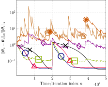
(a)

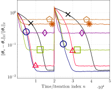
(b)

Fig. 1: : Algorithm 1 ($\alpha=0.9$). Markers , , , , correspond to (1) w/ $p=1,1.25,1.5,1.75,2$, respectively. Marker denotes the algorithm which randomly chooses $p$, $\forall n$.

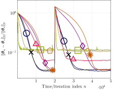
(a)

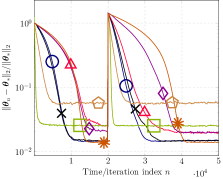
(b)

Fig. 2: : Algorithm 1 ($\alpha=0.9$). : OBR ($\alpha=0.9$) [11]. : Kernel-based TD(0) ($\alpha=0.9$) [18]. : [29] ($p=1,\gamma_{1}=0.9,\gamma_{2}=0.99$). : KLSPI ($\alpha=0.9$) [10]. : Combination of LMS and sign-LMS[33], : [21].

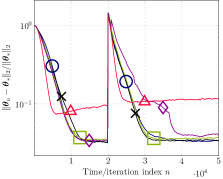
(a)

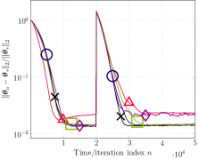
(b)

Fig. 3: Algorithm 1 w/ several parameters. : $\alpha=0.9$. : $\alpha=0.75$. : $\alpha=0$. : OBR ($\alpha=0.9$) [11]. : OBR ($\alpha=0.75$) [11].

References

- [1] D Bertsekas “Reinforcement Learning and Optimal Control” Athena Scientific, 2019
- [2] Richard Ernest Bellman “Dynamic Programming” Dover Publications, 2003
- [3] N Aronszajn “Theory of reproducing kernels” In Transactions of the American Mathematical Society 68, 1950, pp. 337–404
- [4] B Schölkopf and A J Smola “Learning with Kernels: Support Vector Machines, Regularization, Optimization, and Beyond” MIT Press, 2002
- [5] László Györfi, Michael Kohler, Adam Krzyżak and Harro Walk “A Distribution-Free Theory of Nonparametric Regression” New York: Springer, 2010
- [6] H H Bauschke and P L Combettes “Convex Analysis and Monotone Operator Theory in Hilbert Spaces” New York: Springer, 2011
- [7] Robert G Bartle “The Elements of Integration and Lebesgue Measure” John Wiley & Sons, 1995
- [8] Michail G Lagoudakis and Ronald Parr “Least-squares policy iteration” In J. Mach. Learn. Res. 4 JMLR.org, 2003, pp. 1107–1149
- [9] Amir-Massoud Farahmand, Mohammad Ghavamzadeh, Csaba Szepesvári and Shie Mannor “Regularized policy iteration with nonparametric function spaces” In J. Machine Learning Research 17.1, 2016, pp. 4809–4874
- [10] Xin Xu, Dewen Hu and Xicheng Lu “Kernel-based least squares policy iteration for reinforcement learning” In IEEE Transactions on Neural Networks 18.4, 2007, pp. 973–992
- [11] Wen Sun and J Andrew Bagnell “Online Bellman residual and temporal difference algorithms with predictive error guarantees” In Proc. International Joint Conference on Artificial Intelligence, 2016, pp. 4213–4217
- [12] Dirk Ormoneit and Śaunak Sen “Kernel-based reinforcement learning” In Machine Learning 49, 2002, pp. 161–178
- [13] Dirk Ormoneit and Peter Glynn “Kernel-based reinforcement learning in average-cost problems” In IEEE Transactions on Automatic Control 47.10, 2002, pp. 1624–1636
- [14] Andre Barreto, Doina Precup and Joelle Pineau “Reinforcement learning using kernel-based stochastic factorization” In Proc. NIPS 24, 2011
- [15] Andre Barreto, Doina Precup and Joelle Pineau “On-line reinforcement learning using incremental kernel-based stochastic factorization” In Proc. NIPS 25, 2012
- [16] Branislav Kveton and Georgios Theocharous “Structured kernel-based reinforcement learning” In Proc. AAAI Conference on Artificial Intelligence 27, 2013, pp. 569–575
- [17] Branislav Kveton and Georgios Theocharous “Kernel-based reinforcement learning on representative states” In Proc. AAAI Conference on Artificial Intelligence 26.1, 2021, pp. 977–983
- [18] Jihye Bae et al. “Reinforcement learning via kernel temporal difference” In Proc. IEEE EMBS, 2011, pp. 5662–5665 DOI: 10.1109/IEMBS.2011.6091370
- [19] Yiwen Wang and Jose C Príncipe “Reinforcement learning in reproducing kernel Hilbert spaces” In IEEE Signal Processing Magazine 38.4, 2021, pp. 34–45 DOI: 10.1109/MSP.2021.3076309
- [20] Sridhar Mahadevan et al. “Proximal Reinforcement Learning: A New Theory of Sequential Decision Making in Primal-Dual Spaces” In arXiv:1405.6757 abs/1405.6757, 2014 arXiv: http://arxiv.org/abs/1405.6757
- [21] Minh Vu, Yuki Akiyama and K Slavakis “Dynamic Selection of p-Norm in Linear Adaptive Filtering via Online Kernel-Based Reinforcement Learning” In Proc. IEEE ICASSP, 2023
- [22] A H Sayed “Adaptive Filters” Wiley, 2011 URL: https://books.google.co.jp/books?id=VBaenqIVftUC
- [23] Peter J Rousseeuw and Annick Leroy “Robust Regression and Outlier Detection” Wiley, 1987
- [24] M Shao and C L Nikias “Signal processing with fractional lower order moments: Stable processes and their applications” In Proc. IEEE 81.7, 1993, pp. 986–1010 DOI: 10.1109/5.231338
- [25] Soo-Chang Pei and Chien-Cheng Tseng “Least mean p-power error criterion for adaptive FIR filter” In IEEE Journal on Selected Areas in Communications 12.9, 1994, pp. 1540–1547 DOI: 10.1109/49.339922
- [26] Yegui Xiao, Y Tadokoro and K Shida “Adaptive algorithm based on least mean p-power error criterion for Fourier analysis in additive noise” In IEEE Trans. Signal Process. 47.4, 1999, pp. 1172–1181 DOI: 10.1109/78.752620
- [27] Ercan E Kuruoğlu “Nonlinear least -norm filters for nonlinear autoregressive -stable processes” In Digital Signal Processing 12.1, 2002, pp. 119–142
- [28] C Gentile “The robustness of the p-norm algorithms” In Machine Learning 53, 2003, pp. 265–299
- [29] Ángel Navia-Vazquez and Jerónimo Arenas-Garcia “Combination of recursive least p-norm algorithms for robust adaptive filtering in alpha-stable noise” In IEEE Trans. Signal Process. 60.3, 2012, pp. 1478–1482 DOI: 10.1109/TSP.2011.2176935
- [30] Badong Chen et al. “Smoothed least mean p-power error criterion for adaptive filtering” In Digital Signal Processing 40.C, 2015, pp. 154–163
- [31] Konstantinos Slavakis and Masahiro Yukawa “Outlier-robust kernel hierarchical-optimization RLS on a budget with affine constraints” In Proc. IEEE ICASSP, 2021, pp. 5335–5339
- [32] A Singh and José C Príncipe “Using correntropy as a cost function in linear adaptive filters” In Proc. International Joint Conference on Neural Networks, 2009, pp. 2950–2955
- [33] Jonathon Chambers and Apostolos Avlonitis “A robust mixed-norm adaptive filter algorithm” In IEEE Signal Processing Letters 4.2 IEEE, 1997, pp. 46–48
- [34] T Schaul, J Quan, I Antonoglou and D Silver “Prioritized experience replay” In Proc. International Conference on Learning Representations, 2016
- [35] Marc G Bellemare et al. “Increasing the action gap: New operators for reinforcement learning” In Proc. AAAI Conference on Artificial Intelligence 30.1, 2016 DOI: 10.1609/aaai.v30i1.10303
- [36] Steffen Grunewalder et al. “Modelling transition dynamics in MDPs with RKHS embeddings” In arXiv preprint arXiv:1206.4655, 2012
- [37] Ali Rahimi and Benjamin Recht “Random features for large-scale kernel machines” In Proc. NIPS 20, 2007
- [38] José María Miotto “Pylevy”, https://github.com/josemiotto/pylevy, 2020