The muon parton distribution functions

Abstract

We compute the Parton Distribution Functions (PDFs) of the unpolarised muon for the leptons, the photon, the light quarks, and the gluon. We discuss in detail the issues stemming from the necessity of evaluating the strong coupling constant at scales of the order of the typical hadron mass, and compare our novel approach with those currently available in the literature. While we restrict our phenomenological results to be leading-logarithmic accurate, we set up our formalism in a way that renders it straightforward to achieve next-to-leading logarithmic accuracy in the QED, QCD, and mixed QED$\times$QCD contributions.

1 Introduction

The post-LHC generation of high-energy physics experiments will most likely be at lepton colliders. The vast majority of extensive feasibility studies for such colliders have been, and are, carried out by assuming electron/positron beams, with either a circular or a linear geometry. An interesting alternative option is that of a $\mu^{+}\mu^{-}$ collider; while the technical difficulties of controlling and accelerating muon beams remain significant, so are the benefits stemming from building such a machine. Among these, a prominent one is the possibility of achieving much larger c.m. energies w.r.t. those relevant to $e^{+}e^{-}$ colliders with much smaller rings; to be definite, we shall assume that at the typical $\mu^{+}\mu^{-}$ accelerator one will have $\sqrt{s}={\cal O}(1-10~{}{\rm TeV})$.

Because of the large collider energy, the incoming muons are expected to copiously radiate before initiating the hard process; in fact, the particles produced during this radiation phase may eventually undergo hard collisions themselves. Thus, the situation is quite analogous to that of hadronic collisions, and indeed production processes can be described in the same manner, namely by means of a collinear-factorisation formula

$$\sigma_{\mu^{+}\mu^{-}\to X}(s)=\sum_{ij}\int dz_{1}dz_{2}\Gamma_{\!i/\mu^{+}}(z_{1})\Gamma_{\!j/\mu^{-}}(z_{2})\hat{\sigma}_{ij\to X}(z_{1}z_{2}s)\,,$$ (1)

in which process-independent Parton Distribution Functions (PDFs, $\Gamma_{\!i/\mu^{+}}$ and $\Gamma_{\!j/\mu^{-}}$) are convoluted with process-specific short-distance cross sections ($\hat{\sigma}_{ij\to X}$), in which partons ($i$ and $j$) that emerge from the muon beams collide in the hard process. This picture is of course valid for $e^{+}e^{-}$ collisions as well; the difference between the two is that the larger $\mu^{+}\mu^{-}$ c.m. energies imply that the muon PDFs can be probed at values of their arguments (the “Bjorken $x$”, $z_{1}$ and $z_{2}$ in eq. (1)) which are much smaller than their electron counterparts, since when the outgoing system $X$ is produced in the central region of a detector with an invariant mass squared equal to $Q^{2}$ , then $z_{1,2}\sim\sqrt{Q^{2}/s}$. With that being said, the peculiarity of lepton colliders w.r.t. to hadron ones is that the majority of hard collisions still result in large-invariant mass systems, and are due to partons whose identities are the same as those of the respective beams, i.e. $i=\mu^{+}$ and $j=\mu^{-}$, since $\Gamma_{\!\mu^{\pm}/\mu^{\pm}}(z)\sim\delta(1-z)$. Conversely, when $Q^{2}\ll s$, the production process is generally initiated by partons whose identities are different w.r.t. those of the respective beams ($i\neq\mu^{+}$ and $j\neq\mu^{-}$), since for these partons the PDFs peak at small $z$’s. We point out that the set of such partons includes the strongly-interacting ones, i.e. the quarks and the gluon.

It is therefore important, in the context of $\mu^{+}\mu^{-}$-collider studies, that muon PDFs be available for all possible parton types. This necessity has recently been addressed by two different groups Han:2020uid ; Han:2021kes ; Garosi:2023bvq , which have essentially used the same approach. In this paper we follow a strategy that differs from that of refs. Han:2020uid ; Han:2021kes ; Garosi:2023bvq in three major aspects; we shall comment in detail about these in sect. 2. The technical features of our work are discussed in sect. 3, and the resulting PDFs are presented in sect. 4, where we also give sample predictions relevant to dijet production. Finally, we conclude and give an outlook on future work in sect. 5.

2 Motivations

There are three defining features of the PDFs of refs. Han:2020uid ; Han:2021kes ; Garosi:2023bvq . Firstly, the strong-coupling constant is set equal to zero for all scales below a certain threshold, $\alpha_{\scriptscriptstyle S}(\mu)=0$ for $\mu\leq Q_{0}$, while above that threshold a perturbative RGE-evolved form is adopted. Secondly, the $W$ and the $Z$ bosons are regarded as partons, and included in the evolution above the EW scale. Thirdly, the evolution starts from leading-order (LO) initial conditions, and is leading-logarithmic (LL) accurate. We shall now comment on these aspects, w.r.t. which our work has significant differences.

As far as the treatment of strong interactions is concerned, one must bear in mind that lepton PDFs are naturally evolved starting from a scale $\mu_{0}$ of the order of the lepton mass, and ideally strictly equal to the mass itself (lest spurious logarithms are generated in the evolution Bertone:2019hks ). By considering strongly-interacting partons, one is therefore in principle forced to evaluate $\alpha_{\scriptscriptstyle S}$ at scales of the same order as $\Lambda_{\rm QCD}$, thus outside of the perturbative domain. As was said before, this problem is circumvented in refs. Han:2020uid ; Han:2021kes ; Garosi:2023bvq by simply switching QCD off below a scale $Q_{0}={\cal O}(1~{}{\rm GeV})$. Obviously, this is a purely technical procedure: no dynamical mechanism is invoked that could result in this behaviour. More concerning, a strategy of this kind can be seen as equivalent to a renormalon-inspired approach whereby $Q_{0}$ is a free parameter whose value is completely unconstrained, and fixed a posteriori in an observable-dependent manner (see e.g. ref. Webber:1998um for a discussion that focuses on cross sections). In the context of PDF evolution it is unclear whether such a potential dependence on the observable destroys PDF universality and, more pragmatically, how the value of $Q_{0}$ should be chosen (ref. Han:2021kes sets $Q_{0}=0.5$ GeV and considers $Q_{0}=0.7$ GeV as an alternative option, whereas in ref. Garosi:2023bvq variations in the range $0.52\leq Q_{0}\leq 1$ GeV are explored, the default value being $Q_{0}=0.7$ GeV). In this paper, we instead adopt a simple analytical parametrisation Webber:1998um of $\alpha_{\scriptscriptstyle S}$ which is valid for any non-null scale value and is inspired by a dispersive approach; we shall discuss this in sect. 3.1.

For what concerns the heavy EW vector bosons $V=W,Z$, we remind the reader that the argument for treating them as partons amounts essentially to saying that, since $m_{V}^{2}\ll s$, one is in a regime of collinear dominance, where the boson mass is negligible, and its role is thus similar to that of any light particle. In fact, the actual condition is whether $m_{V}^{2}\ll Q^{2}$ or not, where $Q^{2}$ is the invariant mass squared of the system produced in the hard collision. However, as was discussed in sect. 1, for partons different from the muon (therefore including the vector bosons), the cross section associated with invariant masses of the order of the c.m. energy is very small, being strongly suppressed by the $z\to 1$ behaviour of the PDFs themselves. In order to be slightly more quantitative, let us consider the typical figure of merit of collinear physics, which in the case of a vector boson $V$ reads $\alpha_{\scriptscriptstyle W}/\pi\log(Q^{2}/m_{V}^{2})$. For this to have, say, the same value ($0.067$) as its analogue $\alpha/\pi\log(s/m_{e}^{2})$ relevant to an electron in a $\sqrt{s}=350$ GeV collision (i.e. at the FCC-ee) one needs $\sqrt{Q^{2}}\sim 2$ TeV. The c.m. energy required for this value of $Q^{2}$ to correspond to a non-negligible cross section depends of course on the process considered, but an average rough estimate would lead to tens of TeV’s (see e.g. fig. 1 of ref. Han:2021kes ). This is in fact compatible with observations made elsewhere (see e.g. refs. Bauer:2017isx ; Ruiz:2021tdt ) that for true collinear dominance to be achieved in the case of massive vector bosons, and thus for resummation to be necessary, the energies involved need to be much larger than those suggested by naive logarithmic counting. We also point out that with $\sqrt{Q^{2}}=2$ TeV one has $m_{V}^{2}/Q^{2}\sim 2\!\cdot\!10^{-3}$; for comparison, $(\alpha_{\scriptscriptstyle W}/\pi)^{2}\sim 1.1\!\cdot\!10^{-4}$: in other words, power-suppressed effects are larger than the coupling-constant factor of a $2\to 2+n$ process relative to a $2\to n$ one. Finally, we mention the fact that the inclusion of EW heavy bosons in the set of partons implies that the evolution above the EW is carried out in the unbroken EW phase. The practical consequence of this is that there will exist PDFs associated with non-standard objects, namely the “$Z/\gamma$ interference”, that are meant to be convoluted with interference matrix elements (i.e. whose amplitudes on the left- and right-hand side of the cut differ); matrix elements of the latter kind are presently not readily available in codes that compute short-distance cross sections (see however refs. Bothmann:2020sxm ; Pagani:2021vyk ; Pagani:2023wgc for recent progress). For all these reasons, in our approach we do not treat the EW heavy vector bosons as partons, and we do not include them in the evolution of our muon PDFs, regardless of the scale considered.

Finally, refs. Han:2020uid ; Han:2021kes ; Garosi:2023bvq work at the LO+LL precision. This implies that the only non-null initial condition is that of the muon (equal to $\delta(1-z)$), with all of the other PDFs generated dynamically, with evolution equations based on ${\cal O}(\alpha)$ and ${\cal O}(\alpha_{\scriptscriptstyle S})$ splitting kernels. While presently this is a sufficiently pragmatic choice (to which we shall also adhere for our phenomenological predictions), a future increase of accuracy may prove very demanding, since it will entail the computation of the next-to-leading order (NLO) splitting kernels relevant to the heavy-boson sector. Conversely, our approach is based on a simpler QED+QCD evolution, for which all of the required kernels and initial conditions are available at least to NLO; we can thus easily obtain NLO+NLL-accurate predictions. Importantly, an additional benefit of that is the capability of studying explicitly the small-$x$ behaviour of the PDFs.

We conclude this section with an aside that concerns the assumptions on small-scale physics that enter the muon-PDFs determination. If one focuses on the strongly-interacting partons, it may be tempting to describe them as the convolution of the photon quark and gluon PDFs with a function that gives the collinear-photon content of the muon. The latter would be the Weizsäcker-Williams function vonWeizsacker:1934nji ; Williams:1934ad , or any other Equivalent Photon Approximation (EPA), while the former ones would be taken from available fits (for those currently relevant, see e.g. refs. Gluck:1991jc ; Schuler:1995fk ; Schuler:1996fc ; Cornet:2004nb ; Slominski:2005bw ). The underlying idea here is that, thanks to their data-driven determinations, photon PDFs would bypass the necessity of a theoretical modeling of the small-scale behaviour of $\alpha_{\scriptscriptstyle S}$. Unfortunately, such a strategy suffers from severe drawbacks that prevent one from using it in practice. In particular, the quality of photon-PDF fits is generally rather poor, thus inducing systematic uncertainties comparable to or larger than those stemming from the assumptions on $\alpha_{\scriptscriptstyle S}$ in the infrared region. Furthermore, EPAs cannot describe the full complexity of the photon content of a lepton at arbitrary scales (for a discussion specific to this point, see e.g. sect. 4.2.3 of ref. Frixione:2019lga ). In addition to this, it is necessary to bear in mind that the partonic contents of the muon are still predominantly given by the muon itself and the photon, while the presence of the other charged leptons must be taken into account too. It is unclear how to combine the evolution of these partons with that of the strongly-interacting partons originating from the mechanism sketched above. Even if successful, such a combination would entail evaluating the photon PDFs at scales of the order of the muon mass, which poses the very problem one sought to avoid in the first place when introducing these PDFs; obviously, this is true regardless of the quality of the photon-PDF fits, and thus applies even if that quality were to improve in the future. For all of these reasons, we deem that the usage of photon PDFs is not adequate for obtaining reliable muon PDFs, and we shall not discuss this approach any further in this paper.

3 Technicalities

We obtain the muon PDFs by following the same procedure as in refs. Bertone:2019hks ; Bertone:2022ktl : the evolution equations are written in terms of an evolution operator and of the initial conditions in Mellin space, solved there, and inverted numerically back to the $z$ space. The only differences w.r.t. what has been done in refs. Bertone:2019hks ; Bertone:2022ktl are: a) the inclusion of the ${\cal O}(\alpha_{\scriptscriptstyle S})$ splitting kernels; b) the addition of the gluon as an active parton. Furthermore, we neglect the contributions of the ${\cal O}(\alpha^{2})$ splitting kernels, since these are on the same footing as their ${\cal O}(\alpha_{\scriptscriptstyle S}^{2})$ and ${\cal O}(\alpha\alpha_{\scriptscriptstyle S})$ counterparts, which we ignore here. These changes do not entail any conceptual modifications w.r.t. refs. Bertone:2019hks ; Bertone:2022ktl , and only a few minor practical ones; more details are given in sect. 3.2. For consistency, we use LO initial conditions, but we note that the ${\cal O}(\alpha)$ (i.e. NLO) ones computed in ref. Frixione:2019lga do not require any changes when strong interactions are included (the effects of the latter being of ${\cal O}(\alpha\alpha_{\scriptscriptstyle S})$ or higher). We take into account all parton-mass thresholds: each parton participates in the evolution only at and above the corresponding threshold, set equal to its mass (whose value is in turn that of the PDG Zyla:2020zbs ), as is done in ref. Bertone:2022ktl ; the starting scale of the evolution $\mu_{0}$ is set equal to the muon mass. Finally, lest the stability of the results be degraded, at large $z$’s we switch from the numerical to the analytical solution, and are thus able to obtain a smooth behaviour in the whole $z\in(0,1)$ range; we point out that the analytical $z\to 1$ solutions of refs. Bertone:2019hks ; Bertone:2022ktl are unchanged when including strong interactions (both at the LL and the NLL accuracy).

3.1 QCD at small scales

The setup just described, in particular the fact that $\mu_{0}=m_{\mu}$ and the inclusion of the ${\cal O}(\alpha_{\scriptscriptstyle S})$ splitting kernels, requires that $\alpha_{\scriptscriptstyle S}(\mu)$ be computed for any $\mu\geq m_{\mu}$. As was anticipated in sect. 2, we are able to do so by adopting the analytical parametrisation of $\alpha_{\scriptscriptstyle S}$ of ref. Webber:1998um . We point out that, as for all approaches that assume a universal small-scale behaviour of $\alpha_{\scriptscriptstyle S}$, this is expected to induce power-suppressed corrections of ${\cal O}(\Lambda_{\rm QCD}^{2p}/Q^{2p})$ to observables which, given the typical values of $Q^{2}$ relevant to $\mu^{+}\mu^{-}$ collisions, we shall safely neglect here. At the same time, using e.g. a dispersive approach Dokshitzer:1995qm , one sees that the singular behaviour of QCD structure functions is unaffected Dasgupta:1996hh by the small-scale behaviour of $\alpha_{\scriptscriptstyle S}$, and thus that the evolution equations are unchanged.

As far as the strong coupling constant is concerned, for a better phenomenological treatment we use the two-loop QCD $\beta$ function:

$$\beta_{{\rm QCD}}(\alpha_{\scriptscriptstyle S})=-b_{0}\alpha_{\scriptscriptstyle S}^{2}-b_{1}\alpha_{\scriptscriptstyle S}^{3}+{\cal O}(\alpha_{\scriptscriptstyle S}^{4})\,,$$ (2)

with

$$b_{0} = \frac{11C_{\scriptscriptstyle A}-2N_{\scriptscriptstyle F}}{12\pi}\,,$$ (3)

$$b_{1} = \frac{17C_{\scriptscriptstyle A}^{2}-5C_{\scriptscriptstyle A}N_{\scriptscriptstyle F}-3C_{\scriptscriptstyle F}N_{\scriptscriptstyle F}}{24\pi^{2}}\,,$$ (4)

and the number of flavours $N_{\scriptscriptstyle F}$ is understood to be that relevant to the scale range one is working in. Thus, $N_{\scriptscriptstyle F}=5$ for $\mu>m_{b}$, $N_{\scriptscriptstyle F}=4$ for $m_{c}<\mu<m_{b}$, and $N_{\scriptscriptstyle F}=3$ for $\mu_{0}<\mu<m_{c}$ (note that following refs. Bertone:2022ktl ; Zyla:2020zbs we assume $m_{s}<m_{\mu}$). The exact solution for $\alpha_{\scriptscriptstyle S}(\mu)$ of the RGE stemming from eq. (2) is:

$$\int_{\alpha_{\scriptscriptstyle S}^{f}}^{\alpha_{\scriptscriptstyle S}^{\rm RGE}(\mu)}\frac{da}{\beta_{{\rm QCD}}(a)}=\log\frac{\mu^{2}}{\mu_{f}^{2}}\,,$$ (5)

where $\alpha_{\scriptscriptstyle S}^{f}$ is the input value of the coupling constant at the reference scale $\mu_{f}$. The coupling constant to be used in the full scale range $\mu_{0}<\mu<\infty$ is defined as the sum of a perturbative and a non-perturbative part:

$$\alpha_{\scriptscriptstyle S}(\mu)=\alpha_{\scriptscriptstyle S}^{\rm pert}(\mu)+\alpha_{\scriptscriptstyle S}^{\rm np}(\mu)\,.$$ (6)

As far as the former is concerned, we use:

$$\alpha_{\scriptscriptstyle S}^{\rm pert}(\mu)=\left\{\begin{array}[]{ll}1\Big{/}\Big{(}b_{0}\log\big{[}y(\mu)\big{]}\Big{)}&\phantom{aaaaaa}\mu<\mu_{\rm pert}\\ \alpha_{\scriptscriptstyle S}^{\rm RGE}(\mu)&\phantom{aaaaaa}\mu>\mu_{\rm pert}\\ \end{array}\right.\,,$$ (7)

while for the non-perturbative part, we use:

$$\alpha_{\scriptscriptstyle S}^{\rm np}(\mu) = \left\{\begin{array}[]{ll}\frac{1}{b_{0}}a^{\rm np}(y(\mu))&\phantom{aaaaaa}\mu<\mu_{\rm pert}\\ 0&\phantom{aaaaaa}\mu>\mu_{\rm pert}\\ \end{array}\right.\,,$$ (10)

$$a^{\rm np}(y) = \frac{y+b}{(1-y)(1+b)}\left(\frac{1+c}{y+c}\right)^{p}\,,$$ (11)

where $b$, $c$, and $p$ are free, low-energy parameters, The auxiliary functions $x(\mu)$ and $y(\mu)$ are:

$$y(\mu)=x(\mu)\left[1+\left(\frac{\log x(\mu)}{2\pi}\right)^{2}\right]^{\frac{b_{1}}{2b_{0}^{2}}}\,,\;\;\;\;\;\;\;\;x(\mu)=\frac{\mu^{2}}{\Lambda_{\rm QCD}^{2}}\,,$$ (12)

where $\Lambda_{\rm QCD}$ is implicitly defined as follows:

$$\alpha_{\scriptscriptstyle S}^{f}=\frac{1}{b_{0}\log\big{[}y(\mu_{f})\big{]}}+\frac{1}{b_{0}}\,a^{\rm np}(y(\mu_{f}))\,.$$ (13)

All of the above can be restricted to one-loop accuracy by formally setting $b_{1}=0$ everywhere.

We point out that the upper forms in eqs. (7) and (10) guarantee a continuous and smooth behaviour of $\alpha_{\scriptscriptstyle S}(\mu)$ at the Landau pole $\mu=\Lambda_{\rm QCD}$, so they must be adopted at small scales. Conversely, at large scales the difference w.r.t. the exact RGE solution may be noticeable, and for this reason we have introduced the scale $\mu_{\rm pert}$ at which we switch from one functional form to the other. In practice, it is convenient to set $\mu_{\rm pert}$ equal to one of the quark-mass thresholds: of the two possible sensible options ($m_{c}$ and $m_{b}$) we choose the former: $\mu_{\rm pert}=m_{c}$ henceforth. With this, we proceed as follows: we start by setting $\alpha_{\scriptscriptstyle S}^{f}=0.118$ at $\mu_{f}=m_{\scriptscriptstyle Z}\equiv 91.18$ GeV; with $N_{\scriptscriptstyle F}=5$, this determines $\alpha_{\scriptscriptstyle S}^{\rm RGE}(\mu)\equiv\alpha_{\scriptscriptstyle S}(\mu)$ for any $\mu\geq m_{b}$ by means of eq. (5). When then iterate the procedure by setting $\alpha_{\scriptscriptstyle S}^{f}=\alpha_{\scriptscriptstyle S}^{\rm RGE}(\mu_{f})$ at $\mu_{f}=m_{b}$, so as to obtain $\alpha_{\scriptscriptstyle S}(\mu)$ in $m_{c}\leq\mu<m_{b}$ by solving again eq. (5) with $N_{\scriptscriptstyle F}=4$. We now switch to the upper forms in eqs. (7) and (10) and, by setting $\mu_{f}=m_{c}$, $\alpha_{\scriptscriptstyle S}^{f}=\alpha_{\scriptscriptstyle S}^{\rm RGE}(\mu_{f})$, and $N_{\scriptscriptstyle F}=3$, we determine $\Lambda_{\rm QCD}$ with eq. (13), after fixing the low-energy parameters as is indicated in the “def” column of table 1 Webber:1998um . This allows us to obtain $\alpha_{\scriptscriptstyle S}(\mu)$ in $m_{s}\leq\mu<m_{c}$, and therefore to iterate the procedure just described, with the $N_{\scriptscriptstyle F}=2$ value of $\Lambda_{\rm QCD}$ determined after setting $\mu_{f}=m_{s}$ and $\alpha_{\scriptscriptstyle S}^{f}=\alpha_{\scriptscriptstyle S}(\mu_{f})$. The procedure terminates with the matching conditions imposed at the down-quark threshold. In other words, we do not impose any matching conditions at the up-quark threshold (the up quark being the lightest of the quarks with our settings), and therefore the parameters of $\alpha_{\scriptscriptstyle S}$ have the same values for $\mu\in(0,m_{u})$ as for $\mu\in(m_{u},m_{d})$. We point out that the computation of $\alpha_{\scriptscriptstyle S}(\mu)$ for any value $\mu<m_{\mu}$ would be (indirectly) relevant to the muon PDFs only if we aimed at extracting the low-energy parameters of eq. (11) from data (see eq. (14)), which we do not in this work. On the other hand, what was done above allows one to use, without any modifications, this form of $\alpha_{\scriptscriptstyle S}(\mu)$ when including QCD effects in the PDFs of the electron (which we shall not do here).

	def	do1	do2	up1	up2
$b$	0.25	0.2125	0.2875	0.2875	0.2125
$c$	4	4.6	4.6	3.4	3.4
$p$	4	4	4	4	4

Table 1: Values of the non-perturbative parameters that appear in eq. (11). Those in the first column are the default ones; the other columns report the variations we consider in this work.

There are a number of practical, as opposed to conceptual, differences w.r.t. what has been done in ref. Webber:1998um . In particular, we work here at the two-loop level, rather than at the one-loop one; we implement mass thresholds and continuity conditions at them; and we use the exact RGE solution for the perturbative part of coupling constant for scales larger than the charm mass. Conversely, the low-energy parameters $b$, $c$, and $p$ have the same default values as in ref. Webber:1998um . This does not need to be so, and in principle these parameters should be fitted to experimental data. This is outside of the scope of the present work; however, we remark that in ref. Webber:1998um a general compatibility (within ${\cal O}(20\%)$ uncertainties) with event-shape and structure functions data is established by computing the $(a,b)=(1,1)$ and $(2,1)$ moments of $\alpha_{\scriptscriptstyle S}$ according to the definition

$$F_{a,b}(\mu)=\frac{a}{\mu^{a}}\int_{0}^{\mu}\frac{d\kappa}{\kappa}\kappa^{a}\Big{[}\alpha_{\scriptscriptstyle S}(\kappa)\Big{]}^{b}$$ (14)

at $\mu=2$ GeV. In view of this, we have computed the same moments for different scenarios; we report the results in table 2.

	LO(a)	LO(b)	LO(c)	def	do1	do2	up1	up2
$F_{1,1}(2~{}{\rm GeV})$	0.511	0.417	0.543	0.469	0.440	0.455	0.504	0.487
$F_{2,1}(2~{}{\rm GeV})$	0.450	0.344	0.497	0.400	0.393	0.395	0.406	0.404

Table 2: Values of the first two moments of $\alpha_{\scriptscriptstyle S}$ for various settings of the low-energy parameters. See the text for details.

The LO(a) column results from performing the same computation as in ref. Webber:1998um : one-loop $\beta$ function, with $N_{\scriptscriptstyle F}=3$ evolution from $\alpha_{\scriptscriptstyle S}(m_{\scriptscriptstyle Z})=0.118$; we find perfect agreement with table 1 of that paper. For the LO(b) and LO(c) columns we also use a one-loop $\beta$ function, but we now implement continuity conditions at the charm and bottom thresholds, starting with an $N_{\scriptscriptstyle F}=5$ evolution at the $Z$ mass and setting there $\alpha_{\scriptscriptstyle S}(m_{\scriptscriptstyle Z})=0.118$ and $\alpha_{\scriptscriptstyle S}(m_{\scriptscriptstyle Z})=0.135$, respectively. Since $\alpha_{\scriptscriptstyle S}(m_{\scriptscriptstyle Z})=0.118$ is also the initial condition chosen in ref. Webber:1998um , the difference between the LO(a) and LO(b) results is entirely due to using threshold conditions and the corresponding number of flavours in the latter case, which gives significantly smaller values for the moments. Column LO(c) shows that, in order to increase these moments with a variable-flavour-number evolution, one needs to start from a much larger $\alpha_{\scriptscriptstyle S}(m_{\scriptscriptstyle Z})$ value; this is actually consistent with what is observed when fitting one-loop-evolved hadronic PDFs (see e.g. ref. Yan:2022pzl ). The remaining columns in table 2 report the results obtained with the two-loop, threshold-matched evolution discussed at the beginning of this section; we see that those obtained with the default parameters are slightly smaller than, but within 10% of, those of ref. Webber:1998um .

The bottom line is that, for the present phenomenological needs, the default values of the low-energy parameters that enter the non-perturbative part of $\alpha_{\scriptscriptstyle S}(\mu)$ can be set as is done in ref. Webber:1998um . Again, the ranges in which they can vary are best established by means of comparisons to data. Absent those, a theoretical argument is that of choosing them in a way that prevents $\alpha_{\scriptscriptstyle S}(\mu)$ from being larger than one or smaller than zero (neither of which conditions is guaranteed a priori by eq. (11)). By using this argument while fixing the value of $p$ (so as to have an extremely sharp decrease of power-suppressed effects) we end up by tolerating $\pm 15\%$ variations w.r.t. the default values of the $b$ and $c$ parameters. These variations can be combined in the same or in opposite directions, resulting in the four possible scenarios denoted by “do1”, “do2”, “up1”, and “up2” in table 1. These lead to the predictions for the first two moments of $\alpha_{\scriptscriptstyle S}$ reported in the four rightmost columns of table 2.

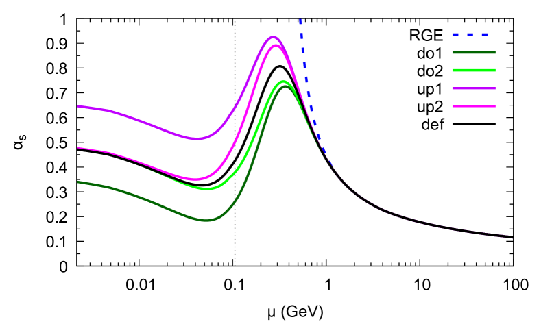
Figure 1: Strong coupling constant as a function of the scale (in GeV), for various choices of the low-energy parameters. The vertical dotted line indicates the value of the muon mass: for this work, only the values to its right are relevant. See the text for details.

The behaviour of $\alpha_{\scriptscriptstyle S}(\mu)$ as a function of $\mu$ is shown in fig. 1, for $\mu>m_{u}$. The five solid lines are the results for $\alpha_{\scriptscriptstyle S}(\mu)$ as is defined in eq. (6), while the dashed line is the result of the solution $\alpha_{\scriptscriptstyle S}^{\rm RGE}(\mu)$ of the perturbative RGE equation (5). The solid lines correspond to the different choices of the non-perturbative parameters of table 1: black for default, dark green for do1, light green for do2, dark magenta for up1, and light magenta for up2. From the figure and the results of table 2 we infer that the low-energy parameter variations we consider in this paper are quite conservative, and likely overestimate the true uncertainty of the analytical model adopted for the strong coupling constant.

3.2 PDF evolution

Following the notation introduced in ref. Bertone:2022ktl , we adopt an evolution basis with a 5-dimensional singlet sector, plus 13 non-singlet functions. For factorisation and renormalisation schemes both chosen equal to $\overline{\rm MS}$, we write the splitting kernels relevant to the non-singlet and singlet evolution as follows

$$P(x,\mu)=\sum_{i=0}^{\infty}\sum_{j=0}^{\infty}\left(\frac{\alpha_{\scriptscriptstyle S}(\mu)}{2\pi}\right)^{i}\left(\frac{\alpha(\mu)}{2\pi}\right)^{j}P^{(i,j)}(x)\,,$$ (15)

$${\mathbb{P}}(x,\mu)=\sum_{i=0}^{\infty}\sum_{j=0}^{\infty}\left(\frac{\alpha_{\scriptscriptstyle S}(\mu)}{2\pi}\right)^{i}\left(\frac{\alpha(\mu)}{2\pi}\right)^{j}{\mathbb{P}}^{(i,j)}(x)\,,$$ (16)

respectively. As is customary, the coefficients on the r.h.s. of eqs. (15) and (16) can be further decomposed into their valence and sea components, by means of which one defines in turn the standard $\pm$ combinations.

With this notation, each of the non-singlet PDFs evolve according to:

$$\frac{\partial\Gamma_{\!a}}{\partial\log\mu^{2}}=P_{a}\otimes\Gamma_{\!a}$$ (17)

which applies to the following $13$ cases when $\mu>m_{b}$ (since there we consider the evolution with $N_{l}=3$ lepton, $N_{u}=2$ up-type quarks, and $N_{d}=3$ down-type quarks, denoted collectively by $f$ in the last line of eq. (18)),

$$\begin{array}[]{rclcc}\Gamma_{\!a}&&&\phantom{aaa}\longleftrightarrow\phantom{aaa}&P_{a}\\ \hline\cr\Gamma_{\!l2}&\;=&\Gamma_{\!e^{-}}+\Gamma_{\!e^{+}}-\left(\Gamma_{\!\mu^{-}}+\Gamma_{\!\mu^{+}}\right)&\phantom{aaa}\longleftrightarrow\phantom{aaa}&P_{l}^{+}\\ \Gamma_{\!l3}&\;=&\Gamma_{\!e^{-}}+\Gamma_{\!e^{+}}+\Gamma_{\!\mu^{-}}+\Gamma_{\!\mu^{+}}-2\left(\Gamma_{\!\tau^{-}}+\Gamma_{\!\tau^{+}}\right)&\phantom{aaa}\longleftrightarrow\phantom{aaa}&P_{l}^{+}\\ \Gamma_{\!uc}&\;=&\Gamma_{\!u}+\Gamma_{\!\bar{u}}-\left(\Gamma_{\!c}+\Gamma_{\!\bar{c}}\right)&\phantom{aaa}\longleftrightarrow\phantom{aaa}&P_{u}^{+}\\ \Gamma_{\!ds}&\;=&\Gamma_{\!d}+\Gamma_{\!\bar{d}}-\left(\Gamma_{\!s}+\Gamma_{\!\bar{s}}\right)&\phantom{aaa}\longleftrightarrow\phantom{aaa}&P_{d}^{+}\\ \Gamma_{\!sb}&\;=&\Gamma_{\!s}+\Gamma_{\!\bar{s}}-\left(\Gamma_{\!b}+\Gamma_{\!\bar{b}}\right)&\phantom{aaa}\longleftrightarrow\phantom{aaa}&P_{d}^{+}\\ \Gamma_{\!f,{\rm\scriptscriptstyle NS}}&\;=&\Gamma_{\!f}-\Gamma_{\!\bar{f}}&\phantom{aaa}\longleftrightarrow\phantom{aaa}&P_{f}^{-}\end{array}\,.$$ (18)

In general, the perturbative coefficients of the $\pm$ combinations of the kernels stemming from eq. (15) that are relevant to eq. (18) are non-null, except for:

$$P_{l}^{\pm(1,0)}=P_{l}^{\pm(2,0)}=P_{l}^{\pm(1,1)}=0\,.$$ (19)

The singlet evolution occurs in a five-dimensional space, that corresponds to the following three linear combinations:

$$\Gamma_{\!\Sigma^{l}} = \sum_{l}^{N_{l}}\left(\Gamma_{\!l^{-}}+\Gamma_{\!l^{+}}\right)\,,$$ (20)

$$\Gamma_{\!\Sigma^{u}} = \sum_{u}^{N_{u}}\left(\Gamma_{\!u}+\Gamma_{\!\bar{u}}\right)\,,$$ (21)

$$\Gamma_{\!\Sigma^{d}} = \sum_{d}^{N_{d}}\left(\Gamma_{\!d}+\Gamma_{\!\bar{d}}\right)\,,$$ (22)

in addition to the photon ($\Gamma_{\!\gamma}$) and gluon ($\Gamma_{\!g}$) densities. It is written thus:

$$\frac{\partial}{\partial\log\mu^{2}}\left(\begin{array}[]{c}\Gamma_{\!\Sigma^{u}}\\ \Gamma_{\!\Sigma^{d}}\\ \Gamma_{\!\Sigma^{l}}\\ \Gamma_{\!\gamma}\\ \Gamma_{\!g}\\ \end{array}\right)={\mathbb{P}}\otimes\left(\begin{array}[]{c}\Gamma_{\!\Sigma^{u}}\\ \Gamma_{\!\Sigma^{d}}\\ \Gamma_{\!\Sigma^{l}}\\ \Gamma_{\!\gamma}\\ \Gamma_{\!g}\\ \end{array}\right),$$ (23)

with the conventions of eq. (16) for the perturbative coefficients. Explicitly, up to the NLO we have:

$${\mathbb{P}}^{(1,0)} = \left(\begin{array}[]{ccccc}P_{q}^{+(1,0)}&0&\phantom{a}0\phantom{a}&\phantom{a}0\phantom{a}&2N_{u}P_{qg}^{(1,0)}\\ 0&P_{q}^{+(1,0)}&0&0&2N_{d}P_{qg}^{(1,0)}\\ 0&0&0&0&0\\ 0&0&0&0&0\\ P_{gq}^{(1,0)}&P_{gq}^{(1,0)}&0&0&P_{gg}^{(1,0)}\\ \end{array}\right),$$ (29)

$${\mathbb{P}}^{(2,0)} = \left(\begin{array}[]{ccccc}P_{q}^{+(2,0)}+2N_{u}P_{qq}^{{\rm S}(2,0)}&2N_{u}P_{qq}^{{\rm S}(2,0)}&0&0&2N_{u}P_{qg}^{(2,0)}\\ 2N_{d}P_{qq}^{{\rm S}(2,0)}&P_{q}^{+(2,0)}+2N_{d}P_{qq}^{{\rm S}(2,0)}&\phantom{a}0\phantom{a}&\phantom{a}0\phantom{a}&2N_{d}P_{qg}^{(2,0)}\\ 0&0&0&0&0\\ 0&0&0&0&0\\ P_{gq}^{(2,0)}&P_{gq}^{(2,0)}&0&0&P_{gg}^{(2,0)}\\ \end{array}\right),$$ (35)

$${\mathbb{P}}^{(0,1)} = \left(\begin{array}[]{ccccc}P_{u}^{+(0,1)}&0&\phantom{a}0\phantom{a}&2N_{u}P_{u\gamma}^{(0,1)}&\phantom{a}0\phantom{a}\\ 0&P_{d}^{+(0,1)}&0&2N_{d}P_{d\gamma}^{(0,1)}&0\\ 0&0&P_{l}^{+(0,1)}&2N_{l}P_{l\gamma}^{(0,1)}&0\\ P_{\gamma u}^{(0,1)}&P_{\gamma d}^{(0,1)}&P_{\gamma l}^{(0,1)}&P_{\gamma\gamma}^{(0,1)}&0\\ 0&0&0&0&0\\ \end{array}\right),$$ (41)

$${\mathbb{P}}^{(0,2)} = \left(\begin{array}[]{ccccc}P_{u}^{+(0,2)}+2N_{u}P_{uu}^{{\rm S}(2,0)}&2N_{u}P_{ud}^{{\rm S}(2,0)}&2N_{u}P_{ul}^{{\rm S}(2,0)}&2N_{u}P_{u\gamma}^{(0,2)}&\phantom{a}0\phantom{a}\\ 2N_{d}P_{du}^{{\rm S}(2,0)}&P_{d}^{+(0,2)}+2N_{d}P_{dd}^{{\rm S}(2,0)}&2N_{d}P_{dl}^{{\rm S}(2,0)}&2N_{d}P_{d\gamma}^{(0,2)}&0\\ 2N_{l}P_{lu}^{{\rm S}(2,0)}&2N_{l}P_{ld}^{{\rm S}(2,0)}&P_{l}^{+(0,2)}+2N_{l}P_{ll}^{{\rm S}(2,0)}&2N_{l}P_{l\gamma}^{(0,2)}&0\\ P_{\gamma u}^{(0,2)}&P_{\gamma d}^{(0,2)}&P_{\gamma l}^{(0,2)}&P_{\gamma\gamma}^{(0,2)}&0\\ 0&0&0&0&0\\ \end{array}\right),$$ (47)

$${\mathbb{P}}^{(1,1)} = \left(\begin{array}[]{ccccc}P_{u}^{+(1,1)}&0&\phantom{a}0\phantom{a}&2N_{u}P_{u\gamma}^{(1,1)}&2N_{u}P_{ug}^{(1,1)}\\ 0&P_{d}^{+(1,1)}&0&2N_{d}P_{d\gamma}^{(1,1)}&2N_{d}P_{dg}^{(1,1)}\\ \phantom{a}0\phantom{a}&0&0&0&0\\ P_{\gamma u}^{(1,1)}&P_{\gamma d}^{(1,1)}&0&P_{\gamma\gamma}^{(1,1)}&P_{\gamma g}^{(1,1)}\\ P_{gu}^{(1,1)}&P_{gd}^{(1,1)}&0&P_{g\gamma}^{(1,1)}&P_{gg}^{(1,1)}\\ \end{array}\right).$$ (54)

The entries of the matrices in eqs. (29)–(54) can be found in, or easily derived from the results of, refs. Curci:1980uw ; Furmanski:1980cm ; Ellis:1996nn ; deFlorian:2015ujt ; deFlorian:2016gvk .

As is shown in refs. Bertone:2019hks ; Frixione:2021wzh ; Bertone:2022ktl , the evolution equation of eq. (23) (and analogously for its non-singlet counterparts of eq. (17)) is conveniently solved in Mellin space, where it is re-expressed in terms of an evolution operator, thus:

$$\frac{\partial{\mathbb{E}}_{N}^{(K)}(\mu)}{\partial\log\mu^{2}}={\mathbb{M}}_{N}^{(K)}(\alpha(\mu),\alpha_{\scriptscriptstyle S}(\mu))\,{\mathbb{E}}_{N}^{(K)}(\mu)\,,$$ (55)

where the index $K$ understands a dependence on the chosen factorisation scheme (see refs. Frixione:2019lga ; Frixione:2021wzh for more details). We stress that the evolution kernel ${\mathbb{M}}_{N}^{(K)}$ coincides with the Mellin transform of the matrix ${\mathbb{P}}$ that appears in eq. (23) (or with its scalar counterparts $P_{a}$ that appear in eq. (17) for the non-singlet densities) only if the factorisation and renormalisation schemes are both chosen equal to $\overline{\rm MS}$ – in all of the other cases, ${\mathbb{M}}_{N}^{(K)}$ is constructed starting from ${\mathbb{P}}$ following the procedure described in refs. Frixione:2021wzh ; Bertone:2022ktl . Furthermore, the kernel ${\mathbb{M}}_{N}^{(K)}$ depends on parameters whose values are determined by the mass range one considers, and specifically by the number of lepton and light-quark flavours which are active there. Therefore, eq. (55) is solved in the range $\mu_{I}<\mu<m_{k}$, with $m_{k}$ a fermion threshold, and $\mu_{I}=\max(\mu_{0},m_{k-1})$, starting with a $k$ value for which $\mu_{I}=\mu_{0}$, and with continuity conditions imposed at the thresholds.

As far as such a solution is concerned, we note that eq. (55) has the same structure as its counterpart in ref. Bertone:2022ktl , except for the fact that it differs from the latter in a single practical aspect. Namely, in ref. Bertone:2022ktl we have considered the cases where ${\mathbb{M}}_{N}^{(K)}$ does not depend on $\mu$, neither directly nor through $\alpha(\mu)$ (this corresponds to the $\overline{\rm MS}$ UV-renormalisation scheme where the running of $\alpha$ is neglected); where ${\mathbb{M}}_{N}^{(K)}$ depends on $\mu$ only through $\alpha(\mu)$ (this corresponds to the $\overline{\rm MS}$ UV-renormalisation scheme); and finally where ${\mathbb{M}}_{N}^{(K)}$ has a direct dependence on $\mu$, but $\alpha$ does not run (this corresponds to the $\alpha(m_{\scriptscriptstyle Z})$ and $G_{\mu}$ UV-renormalisation schemes). Thus, here we have to deal with the last possible case not already taken into account in ref. Bertone:2022ktl , namely that where ${\mathbb{M}}_{N}^{(K)}$ has a direct dependence on $\mu$ (through $\alpha_{\scriptscriptstyle S}(\mu)$), and $\alpha$ is running. It turns out that we can still solve the corresponding evolution equation in a similar manner as in ref. Bertone:2022ktl , i.e. by relying on a path-ordered approach. However, we do so in two different ways, that correspond to choosing different evolution variables; the relevant solutions are then used to validate each other by means of mutual cross-checks. The first evolution variable we adopt is:

$$l=\log\frac{\mu^{2}}{\mu^{2}_{I}}\,;$$ (56)

as was already said, $\mu_{I}$ is the lower end of the current mass range. For each value of $l$, we obtain $\mu$ by simply inverting eq. (56), i.e. $\mu^{2}=\mu_{I}^{2}\,\exp(l)$, and we then evaluate both $\alpha(\mu)$ and $\alpha_{\scriptscriptstyle S}(\mu)$. The second evolution variable is:

$$t=\frac{1}{2\pi\beta_{0}}\log\frac{\alpha(\mu)}{\alpha(\mu_{I})}\,,$$ (57)

with $\beta_{0}$ the LO coefficient of the QED $\beta$ function, in the range where the evolution is taking place, defined according to what follows:

$$\frac{d\alpha(\mu)}{d\log\mu^{2}}\equiv\beta_{{\rm QED}}(\alpha)=\beta_{0}\alpha^{2}+\beta_{1}\alpha^{3}+{\cal O}(\alpha^{4})\,.$$ (58)

In this case, we can immediately obtain $\alpha(\mu)$ by inverting eq. (57):

$$\alpha(\mu)=\alpha(\mu_{I})\,e^{2\pi\beta_{0}\,t}\,.$$ (59)

In order to obtain $\alpha_{\scriptscriptstyle S}(\mu)$ for any $\mu>\mu_{I}$, we first solve the QED RGE eq. (58) to obtain $\mu$ from $\alpha(\mu)$

$$\mu^{2}=\mu_{I}^{2}\exp\left[\!B_{{\rm QED}}\Big{(}\alpha(\mu)\Big{)}-B_{{\rm QED}}\Big{(}\alpha(\mu_{I})\Big{)}\right],$$ (60)

with the $B_{{\rm QED}}$ function at the NLO given by

$$B_{{\rm QED}}(a)\equiv\int\frac{da}{\beta_{{\rm QED}}(a)}=-\frac{1}{\beta_{0}a}-\frac{\beta_{1}}{\left(\beta_{0}\right)^{2}}\log\left(\frac{a}{\beta_{0}+a\,\beta_{1}}\right)\,,$$ (61)

and we then evaluate $\alpha_{\scriptscriptstyle S}(\mu)$.

The path-ordered approach relies on a discretised solution, which is explained in details in sect. 5.2. of ref. Bertone:2022ktl . Here, we limit ourselves to mentioning that, in view of the more complicated scale dependence of ${\mathbb{M}}_{N}^{(K)}$ w.r.t. that of the cases studied in ref. Bertone:2022ktl , and of the more extended scale range w.r.t. that relevant to the electron PDFs, we have re-assessed the dependence of the PDFs upon the number of discrete steps by means of which the evolution operator is constructed. Denoting by $n_{k}$ the number of discrete steps in the $k^{th}$ mass-threshold interval, and by $n=\sum_{k}n_{k}$ the total number of steps, we have found very stable solutions with $50\leq n_{k}\leq 1000$ and $1000\leq n\leq 2000$: with these ranges, the muon and photon PDFs exhibit a relative variation of ${\cal O}(10^{-7})$, while for all of the other partons the effect is of ${\cal O}(10^{-5})$. As such, the impact of the variations of these discrete parameters on the PDFs is totally negligible; we point out that this also allows us to conclude that the inclusion of the scale dependence of $\alpha_{\scriptscriptstyle S}$ does not lead to any qualitative or quantitative changes w.r.t. the findings of ref. Bertone:2022ktl .

As was already mentioned, for the phenomenological results presented in this paper we retain only the ${\cal O}(\alpha_{\scriptscriptstyle S})$ and ${\cal O}(\alpha)$ kernels, i.e. those of eqs. (29) and (41) respectively. We also point out that the basis of the non-singlet functions in eq. (18) is only one among several equally sensible choices; we have verified, by also adopting the basis suggested in ref. Bertone:2015lqa , that our results are basis-independent.

4 Results

In this section we present our predictions for the muon PDFs, and for the dijet cross sections that result from them. In particular, we are interested in assessing the uncertainties that stem from the parametrisation of the strong coupling constant at small scales. In order to do this, in addition to our own approach which has been discussed in detail in sect. 3.1, we have also implemented the strategy of refs. Han:2020uid ; Han:2021kes ; Garosi:2023bvq , where $\alpha_{\scriptscriptstyle S}$ is set equal to zero for $\mu\leq Q_{0}$. We shall refer to these two approaches as “analytical” and “truncated”, respectively. In both of these cases, the uncertainties are defined as the envelopes of the variations of the relevant low-energy parameter(s) – for the analytical approach, these are given in table 1, whereas for the truncated approach we take $Q_{0}\in[0.52,1.0]$ GeV Han:2021kes ; Garosi:2023bvq . We point out that there is a fundamental difference between the uncertainties thus computed with the two methods. Namely, while the low-energy-parameter ranges are to a certain extent always arbitrary, the lower end of the $Q_{0}$ range is necessarily an unstable point, since small variations towards lower values induce progressively larger envelopes (as one moves towards the Landau pole of the perturbatively-computed $\alpha_{\scriptscriptstyle S}$); this behaviour has no analogue in the analytical approach we employ in this work.

4.1 Results for the PDFs

In this section we focus on the PDFs as standalone objects. In general, the muon PDF is utterly dominant, and its size dwarfs that of the PDFs of all of the other partons; in this sense, the situation is quite analogous to that of the electron PDFs. However, this statement is only correct at intermediate and large $z$ values: at $z\to 0$, other partons dominate. As was already discussed in sect. 1, the large c.m. energies expected at muon colliders render the $z\to 0$ region quite relevant for certain production processes. Therefore, in view of the fact that this constitutes a novelty w.r.t. what happens at $e^{+}e^{-}$ colliders, we shall concentrate on this $z$ region in the following. However, we stress that our PDFs do treat the large-$z$ region without any approximation or discontinuity, and as their electron counterparts Bertone:2019hks ; Bertone:2022ktl they can be straightforwardly used to study the production of large-mass systems as well.

Before proceeding to show explicit results, we mention a couple of features of the PDFs (with the analytical low-scale approach) that serve as cross checks. Firstly, we find that by not including the ${\cal O}(\alpha_{\scriptscriptstyle S})$ splitting kernels (i.e. by performing a pure-QED LL evolution, with all of the partons except for the gluon, which cannot be generated in this way) the PDFs of all the leptons and of the photon change by a negligible amount (a relative ${\cal O}(10^{-5})$ factor or smaller) w.r.t. to our default ${\cal O}(\alpha_{\scriptscriptstyle S})+{\cal O}(\alpha)$ coupled-evolution PDFs. Conversely, the PDFs of the quarks display relative differences of tens of percent; typically, the inclusion of QCD splitting kernels results in enhancing (depleting) the PDFs at small (large) $z$ values. Overall, and consistently with basic expectations, the enhancement has a much larger effect than the depletion, since quark PDFs decrease with $z$ (see later). Secondly, while by default we use two-loop coupling constants in our evolution, we have verified that, by employing a one-loop expression for $\alpha_{\scriptscriptstyle S}$, the lepton and photon PDFs change by a relative ${\cal O}(10^{-6})$ factor. While the effect on the quark and gluon PDFs is much larger (up to 10% at $\mu=30$ GeV), it is basically driven by the differences between the two RGE solutions for $\alpha_{\scriptscriptstyle S}$ (at $\mu=m_{c}$, the two-loop value of $\alpha_{\scriptscriptstyle S}(\mu)$ is about 17% larger than its one-loop counterpart, if an initial condition $\alpha_{\scriptscriptstyle S}(m_{\scriptscriptstyle Z})=0.118$ is adopted for both evolutions).

	an.	tr.
$\mu^{-}$	$97.8592_{-0.00\%}^{+0.00\%}$	$97.8592_{-0.00\%}^{+0.00\%}$
$\gamma$	$2.0756_{-0.00\%}^{+0.00\%}$	$2.0756_{-0.00\%}^{+0.00\%}$
$\sum l$	$0.0265_{-0.00\%}^{+0.00\%}$	$0.0265_{-0.00\%}^{+0.00\%}$
$\sum q$	$0.0332_{-0.02\%}^{+0.02\%}$	$0.0333_{-0.23\%}^{+0.17\%}$
$g$	$0.0056_{-0.10\%}^{+0.10\%}$	$0.0055_{-1.03\%}^{+1.01\%}$

Table 3: Fractions of momentum carried by the muon, the photon, all of the leptons different from $\mu^{-}$ ($\sum l$), all of the quarks ($\sum q$), and the gluon, computed with the PDFs based on the analytical (left column) and truncated (right column) low-energy approach. The results are obtained at $\mu=m_{\scriptscriptstyle Z}$.

In table 3 we report the fractions of muon momentum carried by either individual partons or combinations of partons, at $\mu=m_{\scriptscriptstyle Z}$. In addition to the central values, we show the fractional uncertainties due to the choices of the low-energy parameters. We note that the central values stemming from the analytical and truncated approaches are essentially identical or very close to each other. In fact, this is an artifact of the definition of the momentum fraction, that weights each PDF by a factor of $z$, which thus suppresses the contributions of the small-$z$ region; as we shall show later, the differences between the two approaches increase with decreasing $z$. One can also observe a reasonable agreement with the results in the last line of table 1 of ref. Han:2021kes , where the same quantities are reported. As far as the uncertainties associated with the low-energy parameters are concerned, for both the analytical and the truncated approach they are negligible for the muon, photon, and lepton contributions. They remain relatively small in the case of the quarks and the gluon; however, what one can see there is that the uncertainties of the truncated approach are about a factor of ten larger than those stemming from the analytical approach, which is an example of the general features discussed at the beginning of sect. 4.

Figure 2: PDFs at $\mu=30$ GeV. The contents of the two panels are identical, the only difference between the two being the variable on the $x$ axis. Apart from the case of $\mu^{+}$, the antifermion PDFs coincide with those of the corresponding fermions, and are not shown. Also not shown is the strange PDF, since it coincides with that of the down. Finally, on these scales the $\mu^{+}$ and $e^{-}$ results cannot be distinguished from one another.

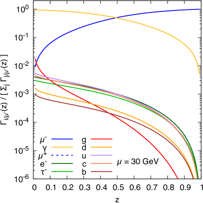
Figure 3: Ratios of individual PDFs over their sum, at $\mu=30$ GeV. The contents of the two panels are identical, the only difference between the two being the variable on the $x$ axis. Apart from the case of $\mu^{+}$, the antifermion PDFs coincide with those of the corresponding fermions, and are not shown. Also not shown is the strange PDF, since it coincides with that of the down. Finally, on these scales the $\mu^{+}$ and $e^{-}$ results cannot be distinguished from one another.

In fig. 2 we show the PDFs of all partons at $\mu=30$ GeV (as a representative scale relevant to the production of a small-mass system) as a function of either $\log_{10}z$ (left panel) or $z$ (right panel). The PDFs are obtained with the analytical low-energy approach, and correspond to the default low-energy parameters. The relative impact of these PDFs is presented in fig. 3, where we plot the ratios of the individual PDFs over the sum of all of them. The plots show clearly the dominance of the muon PDF as $z\to 1$. Conversely, as one moves towards $z=0$, all of the other partons become increasingly important (bar for the non-muon leptons) – still, the muon PDF remains larger than the photon PDF for $z\gtrsim 0.5$, larger than the gluon PDF for $z\gtrsim 0.017$, and larger than the PDF of the largest among the quarks (the up quark) for $z\gtrsim 0.004$. At small $z$ the largest PDF is that of the photon; however, the gluon has the steepest slope of all partons, and in particular its PDF increases faster than the photon one for $z\to 0$. The cumulative impact of the quark PDFs is also non negligible in that region. These facts, coupled with the trivial observation that short-distance cross sections mediated by strong interactions are much larger that those stemming from electroweak interactions, imply that a muon collider constitutes a very favourable environment for clean studies of low-mass hadron-induced systems.

We have considered the same plots as in figs. 2 and 3 for several scales, up to 10 TeV. Qualitatively, we have found the same patterns as at $30$ GeV; quantitatively, in the small-$z$ region the relative impact of the PDFs of the strongly-interacting partons grows with the scale. Having said that, we point out that, given the collider energy, larger scales are mostly associated with larger $z$ values; when such scales are relevant, in order to probe small $z$’s one needs to focus on very boosted systems.

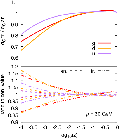
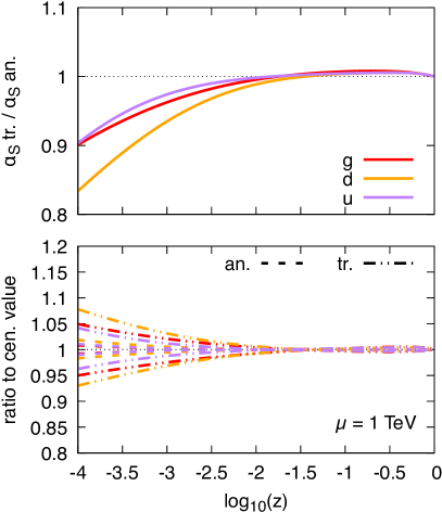
Figure 4: Dependence of the gluon, $u$-quark, and $d$-quark PDFs on the low-energy parameters. See the text for details.

We now turn to consider the dependence of the PDFs on the approach chosen for the small-scale behaviour of $\alpha_{\scriptscriptstyle S}$, as well as that on the relevant low-energy parameters. We summarise our findings in fig. 4; the left-side panels, obtained at $\mu=30$ GeV, have the same layouts as the right-side ones, obtained at $\mu=1$ TeV. The upper panels show the ratio of the PDFs obtained with the default parameters in the truncated approach over their counterparts in the analytical approach. While there are differences among the partons considered, broadly speaking the analytical approach gives larger (smaller) PDFs than the truncated one for $z\lesssim 0.05$ ($z\gtrsim 0.05$). These differences are largest at the smallest $z$ values: e.g. for $z=10^{-4}$, the analytical-approach PDFs are larger than the truncated-approach ones by $20-30$% at $\mu=30$ GeV, and by $10-15$% at $\mu=1$ TeV. This information has to be taken together with that on the uncertainties due to the choices of the low-energy parameters. In the lower panels fig. 4 we display such fractional uncertainties for the analytical (dashed curves) and truncated (dot-dashed curves) approaches; the curves represent the envelopes, computed as was explained at the beginning of sect. 4. One sees here the local (in $z$) version of what has been observed in table 3: the analytical approach gives significantly smaller uncertainties than the truncated one. In both cases, the uncertainties decrease with the scale. We shall soon see (sect. 4.2) the implications of these facts on selected observables.

4.2 Results for dijet cross sections

In this section we report our predictions for dijet total rates. We work with LO short-distance cross sections (i.e. at ${\cal O}(\alpha_{\scriptscriptstyle S}^{n}\alpha^{m})$ with $n+m=2$); as such, jets coincide with partons (i.e. there is no need for a jet-finding algorithm), and are defined by means of the simplest acceptance cuts:

$$p_{\scriptscriptstyle T}^{(j)}>p_{\scriptscriptstyle T}^{cut}\,,\;\;\;\;\;\;\;\;\left|\eta^{(j)}\right|<3\,.$$ (62)

The collider energy is $\sqrt{s}=10$ TeV, and we consider $p_{\scriptscriptstyle T}^{cut}=10$ GeV and $p_{\scriptscriptstyle T}^{cut}=100$ GeV; the factorisation and renormalisation scales are set equal to $p_{\scriptscriptstyle T}^{(j)}$.

We point out that in the presence of EW interactions the definition of the partonic content of a jet constitutes a non-trivial problem (see e.g. ref. Frederix:2016ost for an extended discussion of this matter). By working at the LO most of the complications can be avoided, and we can obtain sensible results by considering only light quarks and gluons when defining the jets. Conversely, since we are working at an $\mu^{+}\mu^{-}$ collider, the initial-state and intermediate partons can be light quarks, gluons, leptons, and photons. In summary, the results of this section have been obtained by employing the $2\to 2$ matrix elements relevant to the processes:

$$p_{1}+p_{2}\;\longrightarrow\;p_{3}+p_{4}\,,$$ (63)

with

$$p_{1}\,,p_{2}\in\big{\{}q_{i},\bar{q}_{i},g,l_{i}^{\pm},\gamma\big{\}}\,,\;\;\;\;\;\;\;\;p_{3}\,,p_{4}\in\big{\{}q_{i},\bar{q}_{i},g\big{\}}\,.$$ (64)

In view of this, the intermediate $s$- or $t$-channel partons are light quarks, gluons, or photons.

$\sigma$($p_{\scriptscriptstyle T}^{cut}=10$ GeV) [pb]	an.	tr.
${\cal O}(\alpha_{\scriptscriptstyle S}^{2})$	$18.33_{-1.25\%}^{+1.30\%}$	$15.00_{-10.99\%}^{+10.23\%}$
$\gamma$-ind.	$8.24_{-0.91\%}^{+0.68\%}$	$7.56_{-3.75\%}^{+3.71\%}$
total	$26.58_{-1.15\%}^{+1.11\%}$	$22.57_{-8.56\%}^{+8.04\%}$

Table 4: Total dijet rates for $p_{\scriptscriptstyle T}^{cut}=10$ GeV, in pb.

$\sigma$($p_{\scriptscriptstyle T}^{cut}=100$ GeV) [fb]	an.	tr.
${\cal O}(\alpha_{\scriptscriptstyle S}^{2})$	$41.38_{-0.03\%}^{+0.03\%}$	$41.17_{-0.85\%}^{+0.46\%}$
$\gamma$-ind.	$90.03_{-0.02\%}^{+0.01\%}$	$89.67_{-0.32\%}^{+0.24\%}$
total	$136.91_{-0.00\%}^{+0.00\%}$	$136.35_{-0.48\%}^{+0.28\%}$

Table 5: Total dijet rates for $p_{\scriptscriptstyle T}^{cut}=100$ GeV, in fb.

The total dijet rates within the acceptance cuts of eq. (62) are given in the last line of tables 4 (for $p_{\scriptscriptstyle T}^{cut}=10$ GeV) and 5 (for $p_{\scriptscriptstyle T}^{cut}=100$ GeV) – note the different units employed in these two tables. In addition to these, we also report the results for the sum of the ${\cal O}(\alpha_{\scriptscriptstyle S}^{2})$ contributions (first line), i.e. of the pure-QCD processes, and for the sum of the photon-induced contributions (second line), i.e. those with $\gamma\gamma$, $\gamma q$, and $\gamma g$ partonic initial states. Thus, the differences between the results in the third line and the sum of their counterparts in the first and second lines is equal to the sum of the ${\cal O}(\alpha^{2})$ contributions of the four-fermion processes.

These results complement, and confirm, those for standalone PDFs that we have discussed in sect. 4.1. In particular: a) the low-energy-parameter uncertainties of the analytical approach are always much smaller than those of the truncated one; b) these uncertainties are significantly larger with $p_{\scriptscriptstyle T}^{cut}=10$ GeV than with $p_{\scriptscriptstyle T}^{cut}=100$ GeV; in the latter case, those stemming from the analytical approach are essentially negligible; c) at $p_{\scriptscriptstyle T}^{cut}=10$ GeV, the central values stemming from the analytical and truncated approaches are fairly different from one another. Moreover, they are not within the low-energy parameter uncertainty ranges; this underscores again the fundamental difference between the two approaches, which plays an increasingly important role as one probes smaller $z$ values, i.e. not only for small-mass systems, but also for those that feature large longitudinal boosts. We conclude with two additional observations. Firstly, the low-energy parameter uncertainties of the photon-induced contributions stem entirely from the corresponding quark- and gluon-PDF uncertainties (i.e. these are negligible in the case of the $\gamma\gamma$ channel; as it was discussed sect. 4.1, the photon PDF is fairly stable against the variations of these parameters). Secondly, the relative impact of the four-fermion contributions grows with $p_{\scriptscriptstyle T}^{cut}$: it is negligible at $p_{\scriptscriptstyle T}^{cut}=10$ GeV, and becomes equal to about 4% of the total at $p_{\scriptscriptstyle T}^{cut}=100$ GeV, where it is overwhelmingly due to the $l^{+}l^{-}$ channels.

5 Conclusions and outlook

We have computed the PDFs of the unpolarised muon in the context of a coupled QED-QCD evolution; the set of partons is constituted by the leptons, the light quarks (including the $c$ and $b$ quarks), the photon, and the gluon. Our work differs in several notable ways w.r.t. those in the literature Han:2020uid ; Han:2021kes ; Garosi:2023bvq that have studied the same topic. Firstly, we adopt a dispersive-inspired parametrisation of $\alpha_{\scriptscriptstyle S}$ that allows one to compute it for any scale values, including those of ${\cal O}(\Lambda_{\rm QCD})$ and below. This implies that the resulting predictions are stable w.r.t. the variations of the low-energy parameters that control the small-scale behaviour of $\alpha_{\scriptscriptstyle S}$, at variance with what happens in the truncated approach of refs. Han:2020uid ; Han:2021kes ; Garosi:2023bvq , which is inherently unstable. An additional benefit of our approach is that its low-energy parameters can be fitted to data (typically, of $e^{+}e^{-}$ event shapes or of hadronic structure functions) without loss of predictive power in the context of $\mu^{+}\mu^{-}$ physics, since they are assumed to underpin the universal features of small-scale $\alpha_{\scriptscriptstyle S}$. Secondly, we do not consider the heavy electroweak vector bosons as partons. In essence, even for collider energies of tens of TeVs, the cases where the boson masses are negligible, and the resummation of the large logarithms they induce is important, are extremely marginal; conversely, vector-boson mass effects are ubiquitous, and this suggests that a treatment based on perturbative matrix-element computations is to be preferred. Thirdly, while in this paper we limit ourselves to presenting LL-accurate predictions, in order to facilitate the comparison with the results of refs. Han:2020uid ; Han:2021kes ; Garosi:2023bvq in terms of the aspects mentioned above, we have shown that an increase of precision does not entail any new conceptual features, and can thus be easily achieved.

From a practical viewpoint, the muon PDFs are computed in the same manner as was done for their electron counterparts in refs. Bertone:2019hks ; Bertone:2022ktl : in particular, they take into account all lepton and light-quark mass thresholds, and are continuous and smooth over the whole $z\in(0,1)$ range. As such, they do not present any qualitatively new feature in the $z\to 1$ region, where the muon-parton PDF is hugely dominant. Because of this, in our phenomenological studies we have only considered the small-$z$ region, either by looking directly at the PDFs, or by computing dijet cross sections with small transverse-momentum cuts. The overall conclusion is that the different treatment of the small-scale behaviour of $\alpha_{\scriptscriptstyle S}$ w.r.t. that of refs. Han:2020uid ; Han:2021kes ; Garosi:2023bvq induces visible difference both for the central values and for the uncertainties associated with low-energy parameter variations, which in our case are significantly smaller.

As a follow-up of this work we shall compute the PDFs at the NLL accuracy in the QED, QCD, and mixed QED$\times$QCD contributions. While interesting in itself, the crucial advantage of our ability to do so is that it gives us the possibility of studying in more detail the small-$z$ behaviour of the PDFs and, if need be, to resum the large logarithmic contributions that potentially arise there.

References

- (1) T. Han, Y. Ma and K. Xie, High energy leptonic collisions and electroweak parton distribution functions, Phys. Rev. D 103 (2021) L031301, [2007.14300].
- (2) T. Han, Y. Ma and K. Xie, Quark and gluon contents of a lepton at high energies, JHEP 02 (2022) 154, [2103.09844].
- (3) F. Garosi, D. Marzocca and S. Trifinopoulos, LePDF: Standard Model PDFs for High-Energy Lepton Colliders, 2303.16964.
- (4) V. Bertone, M. Cacciari, S. Frixione and G. Stagnitto, The partonic structure of the electron at the next-to-leading logarithmic accuracy in QED, JHEP 03 (2020) 135, [1911.12040].
- (5) B. R. Webber, QCD power corrections from a simple model for the running coupling, JHEP 10 (1998) 012, [hep-ph/9805484].
- (6) C. W. Bauer, N. Ferland and B. R. Webber, Standard Model Parton Distributions at Very High Energies, JHEP 08 (2017) 036, [1703.08562].
- (7) R. Ruiz, A. Costantini, F. Maltoni and O. Mattelaer, The Effective Vector Boson Approximation in high-energy muon collisions, JHEP 06 (2022) 114, [2111.02442].
- (8) E. Bothmann and D. Napoletano, Automated evaluation of electroweak Sudakov logarithms in Sherpa, Eur. Phys. J. C 80 (2020) 1024, [2006.14635].
- (9) D. Pagani and M. Zaro, One-loop electroweak Sudakov logarithms: a revisitation and automation, JHEP 02 (2022) 161, [2110.03714].
- (10) D. Pagani, T. Vitos and M. Zaro, Improving NLO QCD event generators with high-energy EW corrections, 2309.00452.
- (11) C. F. von Weizsacker, Radiation emitted in collisions of very fast electrons, Z. Phys. 88 (1934) 612–625.
- (12) E. J. Williams, Nature of the high-energy particles of penetrating radiation and status of ionization and radiation formulae, Phys. Rev. 45 (1934) 729–730.
- (13) M. Gluck, E. Reya and A. Vogt, Photonic parton distributions, Phys. Rev. D 46 (1992) 1973–1979.
- (14) G. A. Schuler and T. Sjostrand, Low and high mass components of the photon distribution functions, Z. Phys. C 68 (1995) 607–624, [hep-ph/9503384].
- (15) G. A. Schuler and T. Sjostrand, Parton distributions of the virtual photon, Phys. Lett. B 376 (1996) 193–200, [hep-ph/9601282].
- (16) F. Cornet, P. Jankowski and M. Krawczyk, A New 5 flavor NLO analysis and parametrizations of parton distributions of the real photon, Phys. Rev. D 70 (2004) 093004, [hep-ph/0404063].
- (17) W. Slominski, H. Abramowicz and A. Levy, NLO photon parton parametrization using ee and ep data, Eur. Phys. J. C 45 (2006) 633–641, [hep-ph/0504003].
- (18) S. Frixione, Initial conditions for electron and photon structure and fragmentation functions, JHEP 11 (2019) 158, [1909.03886].
- (19) V. Bertone, M. Cacciari, S. Frixione, G. Stagnitto, M. Zaro and X. Zhao, Improving methods and predictions at high-energy e+e- colliders within collinear factorisation, JHEP 10 (2022) 089, [2207.03265].
- (20) Particle Data Group collaboration, P. Zyla et al., Review of Particle Physics, PTEP 2020 (2020) 083C01.
- (21) Y. L. Dokshitzer, G. Marchesini and B. R. Webber, Dispersive approach to power behaved contributions in QCD hard processes, Nucl. Phys. B 469 (1996) 93–142, [hep-ph/9512336].
- (22) M. Dasgupta and B. R. Webber, Power corrections and renormalons in deep inelastic structure functions, Phys. Lett. B 382 (1996) 273–281, [hep-ph/9604388].
- (23) xFitter Developers’ Team collaboration, F. Giuli et al., The photon PDF from high-mass Drell–Yan data at the LHC, Eur. Phys. J. C 77 (2017) 400, [1701.08553].
- (24) M. Yan, T.-J. Hou, P. Nadolsky and C. P. Yuan, CT18 global PDF fit at leading order in QCD, Phys. Rev. D 107 (2023) 116001, [2205.00137].
- (25) D. de Florian, G. F. R. Sborlini and G. Rodrigo, Two-loop QED corrections to the Altarelli-Parisi splitting functions, JHEP 10 (2016) 056, [1606.02887].
- (26) G. Curci, W. Furmanski and R. Petronzio, Evolution of Parton Densities Beyond Leading Order: The Nonsinglet Case, Nucl. Phys. B 175 (1980) 27–92.
- (27) W. Furmanski and R. Petronzio, Singlet Parton Densities Beyond Leading Order, Phys. Lett. B 97 (1980) 437–442.
- (28) R. K. Ellis and W. Vogelsang, The Evolution of parton distributions beyond leading order: The Singlet case, hep-ph/9602356.
- (29) D. de Florian, G. F. R. Sborlini and G. Rodrigo, QED corrections to the Altarelli–Parisi splitting functions, Eur. Phys. J. C 76 (2016) 282, [1512.00612].
- (30) S. Frixione, On factorisation schemes for the electron parton distribution functions in QED, JHEP 07 (2021) 180, [2105.06688].
- (31) V. Bertone, S. Carrazza, D. Pagani and M. Zaro, On the Impact of Lepton PDFs, JHEP 11 (2015) 194, [1508.07002].
- (32) R. Frederix, S. Frixione, V. Hirschi, D. Pagani, H.-S. Shao and M. Zaro, The complete NLO corrections to dijet hadroproduction, JHEP 04 (2017) 076, [1612.06548].