$k$-Contraction in a Generalized Lurie System

Abstract

We derive a sufficient condition for $k$-contraction in a generalized Lurie system, that is, the feedback connection of a nonlinear dynamical system and a memoryless nonlinear function. For $k=1$, this reduces to a sufficient condition for standard contraction. For $k=2$, this condition implies that every bounded solution of the closed-loop system converges to an equilibrium, which is not necessarily unique. We demonstrate the theoretical results by analyzing $k$-contraction in a biochemical control circuit with nonlinear dissipation terms.

I Introduction

Contraction theory [25, 9, 1] provides powerful analytical tools for the global analysis of nonlinear systems, and has found applications in numerous fields including neural networks [39, 15], robotics [12, 46, 21, 44], learning theory [50, 7, 44, 40, 19], multi-agent systems [37], nonlinear control [5, 27], systems biology [41, 29, 43], and adaptive control [8, 47]. However, if a contracting system admits an equilibrium then this equilibrium must be unique and globally exponentially stable. Thus, contraction theory cannot be directly applied to systems that admit more than a single equilibrium, such as multi-stable systems that are ubiquitous in many fields of science (see, e.g., [3, 11]). Note though that contraction theory has been extended to other contexts such as synchronization through the use of the so called virtual system [49, 37].

Motivated by the seminal study of Muldowney and Li [32, 23] and closely related works [22, 31], Wu et al. recently developed the notion of $k$-contraction [51], with $k>0$ an integer, and more generally of $\alpha$-contraction [52], with $\alpha>0$ real. Roughly speaking, a system is $k$-contracting if its flow contracts $k$-dimensional bodies. For $k=1$, this reduces to standard contraction. In a time-invariant $2$-contracting system every bounded solution converges to an equilibrium, yet the equilibrium is not necessarily unique. This allows global analysis of nonlinear systems that are not contracting (i.e., not $1$-contracting). More generally, a system is $\alpha$-contracting, with $\alpha$ real, if any attractor has a Hausdorff dimension smaller than $\alpha$ [52]. The main tool used in generalizing contraction to $k$- and $\alpha$-contraction is compound matrices [6].

One of the advantages of contraction theory is that interconnections of contracting subsystems are often contracting overall [25, 42]. However, this property does not generalize directly to $k$-contraction; for example, the series interconnection of two 2-contracting subsystems is not 2-contracting in general [31, 34]. Thus, finding necessary or sufficient conditions under which an interconnection is $k$-contracting is still an open question. Refs. [35, 28] present several sufficient conditions guaranteeing $k$-contraction in parallel and series interconnections, as well as in skew-symmetric feedback interconnections. A small-gain condition guaranteeing 2-contraction in a feedback interconnection is presented in [4]. One reason that proving $k$-contraction in interconnections is difficult is that $k$-compounds of block matrices do not necessarily exhibit an obvious block structure. This challenge is partially addressed in [14] which derives a sufficient condition for $k$-contraction that does not require computing $k$-compounds, at the cost of potentially conservative results. In this work, we consider a specific type of feedback interconnections referred to as a generalized Lurie system. By leveraging this special structure we obtain an explicit and easy to verify sufficient condition for $k$-contraction.

A Lurie system, named after Anatolii Isakovich Lurie [16, 24], is the feedback connection of a linear time-invariant (LTI) dynamical system and a nonlinear function. This may be interpreted as the simplest generalization of the feedback connection of an LTI system and a linear controller. The absolute stability problem is to find conditions guaranteeing asymptotic stability of the closed-loop system for every nonlinear function in some admissible class, e.g., sector bounded functions.

Lurie systems were first studied as a tool to analyze the stability of surfacing submarines [26], but it turns out that many dynamical systems that combine linear and nonlinear dynamics can be represented as a Lurie system. In addition, the analysis of the absolute stability problem led to many important theoretical advances in systems and control theory including the KYP Lemma and passivity-based analysis of interconnected systems [20], and the formulation of an optimal control approach in the stability analysis of switched linear systems (see the survey paper [30]).

Several authors studied the stability of Lurie systems using contraction theory (see, e.g., [2, 17, 38] and also [33] which studies contraction in the more general context of DAEs), but such systems often admit more than one equilibrium, which implies that the system is not contracting with respect to (w.r.t.) any norm. Ref. [36] derived sufficient conditions for $k$-contraction in Lurie systems and demonstrated their applications in the case $k=2$ to several models including recurrent neural networks and opinion dynamics models.

Here, we derive new sufficient conditions for $k$-contraction for a much more general class of systems that we refer to as a generalized Lurie model. Our results generalize earlier works in two important aspects. First, we consider a wider class of systems, where both the dynamic subsystem as well as the memoryless subsystem are nonlinear. This adds significant flexibility in choosing an appropriate Lurie representation for a given closed-loop system, extending the applicability of our earlier sufficient condition for $k$-contraction in [36]. Second, we allow studying $k$-contraction with respect to a state-dependent metric, adding a significant additional degree of freedom [25]. We demonstrate our theoretical results by analyzing the global behaviour of a biochemical control circuit.

This note is organized as follows. Section II reviews some preliminary results that are used in the paper. Section III introduces the generalized Lurie model. Section IV states our main results. The proofs of these results are given in Section V. Section VI describes an application of our theoretical results. The final section concludes and describes possible directions for further research.

We use the following notation. Vectors [matrices] are denoted by small [capital] letters. For a vector $x$ and $1\leq p\leq\infty$, $|x|_{p}$ is the $L_{p}$ norm of $x$. For a matrix $A$, $A^{\mathsf{T}}$ is the transpose of $A$. For a square matrix $A$, $\det(A)$ is the determinant of $A$. $I_{n}$ is the $n\times n$ identity matrix. For a symmetric matrix $A\in\mathbb{R}^{n\times n}$, the eigenvalues of $A$ are

$$\lambda_{1}(A)\geq\lambda_{2}(A)\geq\dots\geq\lambda_{n}(A).$$

A symmetric matrix $A\in\mathbb{R}^{n\times n}$ is called positive definite [positive semi-definite] and denoted $A\succ 0$ [$A\succeq 0$], if $x^{\mathsf{T}}Ax>0$ for any $x\in\mathbb{R}^{n}\setminus\{0\}$ [$x^{\mathsf{T}}Ax\geq 0$ for any $x\in\mathbb{R}^{n}$]. For an integer $k>0$, let $[1,k]=\{1,2,\dots,k\}$. For a differentiable function $f:\mathbb{R}\to\mathbb{R}$, $f^{\prime}(s)$ is the derivative of $f$ at $s$.

II Preliminaries

II-A Compound matrices

The analysis of $k$-contraction and $\alpha$-contraction builds on the $k$-compounds of the Jacobian of the vector field. We briefly review this topic, referring to [6] for more details and proofs.

Given $A\in\mathbb{R}^{n\times m}$ and $k\in[1,\min\{n,m\}]$, the $k$-multiplicative compound matrix of $A$, denoted $A^{(k)}$, is the matrix that includes all the $k$-minors of $A$, ordered lexicographically. Thus, $A^{(k)}$ is $\binom{n}{k}\times\binom{m}{k}$. For example, for

$$A=\begin{bmatrix}a_{11}&a_{12}&a_{13}\\ a_{21}&a_{22}&a_{23}\end{bmatrix}$$

and $k=2$, we have

$$A^{(2)}=\begin{bmatrix}\det\begin{bmatrix}a_{11}&a_{12}\\ a_{21}&a_{22}\end{bmatrix}&\det\begin{bmatrix}a_{11}&a_{13}\\ a_{21}&a_{23}\end{bmatrix}&\det\begin{bmatrix}a_{12}&a_{13}\\ a_{22}&a_{23}\end{bmatrix}\end{bmatrix}.$$

By definition, $A^{(1)}=A$, and if $A\in\mathbb{R}^{n\times n}$ then $A^{(n)}=\det(A)$. Also, $I_{n}^{(k)}=I_{r}$, with $r:=\binom{n}{k}$, and $(A^{(k)})^{\mathsf{T}}=(A^{\mathsf{T}})^{(k)}$.

The Cauchy-Binet theorem asserts that for any $A\in\mathbb{R}^{n\times m}$, $B\in\mathbb{R}^{m\times p}$ and $k\in[1,\min\{n,m,p\}]$, we have

$$(AB)^{(k)}=A^{(k)}B^{(k)}.$$ (1)

This justifies the term multiplicative compound. Note that for $A,B\in\mathbb{R}^{n\times n}$ and $k=n$, this reduces to $\det(AB)=\det(A)\det(B)$. Furthermore, Eq. (1) implies that $A^{(k)}$ is invertible iff $A$ is invertible, and $(A^{(k)})^{-1}=(A^{-1})^{(k)}$.

If $D\in\mathbb{R}^{n\times n}$ is diagonal, that is, $D=\operatorname{diag}(\lambda_{1},\dots,\lambda_{n})$ then $D^{(k)}$ is also diagonal, with

$$D^{(k)}=\operatorname{diag}\left(\prod_{i=1}^{k}\lambda_{i},(\prod_{i=1}^{k-1}\lambda_{i})\lambda_{k+1},\dots,\prod_{i=n-k+1}^{n}\lambda_{i}\right).$$

More generally, the $k$-multiplicative compound of a square matrix $A\in\mathbb{R}^{n\times n}$ has an important spectral property. If $\lambda_{1},\dots,\lambda_{n}$ are the eigenvalues of $A$ then the eigenvalues of $A^{(k)}$ are all the $\binom{n}{k}$ products:

$$\lambda_{i_{1}}\dots\lambda_{i_{k}},\quad 1\leq i_{1}<\dots<i_{k}\leq n.$$

It follows that if $A\succ 0$ [$A\succeq 0$], then $A^{(k)}\succ 0$ [$A^{(k)}\succeq 0$].

The $k$-multiplicative compound has an important geometric interpretation. Fix $k$ vectors $a^{1},\dots,a^{k}\in\mathbb{R}^{n}$. The parallelotope generated by these vectors is

$$\mathcal{P}(a^{1},\dots,a^{k}):=\left\{\sum_{i=1}^{k}c_{i}a^{i}\,|\,c_{i}\in[0,1]\right\}$$

(see Fig. 1). Define the $n\times k$ matrix $V:=\begin{bmatrix}a^{1}&\dots&a^{k}\end{bmatrix}$. Then the volume of $\mathcal{P}(a^{1},\dots,a^{k})$ is equal to $|V^{(k)}|_{2}.$ Note that $V^{(k)}$ has dimensions $\binom{n}{k}\times\binom{k}{k}$, i.e., it is a column vector. In the particular case $k=n$, this gives the well-known expression $\text{volume}(\mathcal{P}(a^{1},\dots,a^{n}))=|\det\begin{bmatrix}a^{1}&\dots&a^{n}\end{bmatrix}|.$

Figure 1: A 3D parallelotope.

To study the evolution of a parallelotope under a dynamical system, consider the linear time-invariant (LTI) system

$$\dot{x}=Ax$$ (2)

and let $x(t,x_{0})$ denote its solution at time $t$ when $x(0)=x_{0}$. Fix initial conditions $a^{1},\dots,a^{k}\in\mathbb{R}^{n}$, and consider the time-varying parallelotope $\mathcal{P}(x(t,a^{1}),\dots,x(t,a^{k})).$ We already know that the volume of this parallelotope is the $L_{2}$ norm of the vector $v(t):=\begin{bmatrix}x(t,a^{1})&\dots&x(t,a^{k})\end{bmatrix}^{(k)}$. Now,

$$\dot{v}(t) =\frac{d}{dt}\big{(}\exp(At)\begin{bmatrix}a^{1}&\dots&a^{k}\end{bmatrix}\big{)}^{(k)}$$

$$=\frac{d}{dt}\left((\exp(At))^{(k)}\begin{bmatrix}a^{1}&\dots&a^{k}\end{bmatrix}^{(k)}\right)$$

$$=\frac{d}{dt}\left((\exp(At))^{(k)}\right)v(0),$$ (3)

where the second equality follows from the Cauchy-Binet theorem.

Eq. (II-A) leads to the notion of the $k$-additive compound of a (square) matrix $A\in\mathbb{R}^{n\times n}$. For $\varepsilon\geq 0$, consider the $\binom{n}{k}\times\binom{n}{k}$ matrix $(I_{n}+\varepsilon A)^{(k)}$. Every entry of this matrix is a $k$-minor of $I_{n}+\varepsilon A$, so we can write

$$(I_{n}+\varepsilon A)^{(k)}=B_{0}\varepsilon^{0}+B_{1}\varepsilon^{1}+\dots+B_{k}\varepsilon^{k}.$$

Note that setting $\varepsilon=0$ gives $B_{0}=I_{r}$, with $r:=\binom{n}{k}$. The matrix $B_{1}$ is called the $k$-additive compound of $A$, denoted $A^{[k]}$. Thus,

$$\frac{d}{dt}(\exp(At))^{(k)}|_{t=0}=\frac{d}{dt}(I_{n}+At)^{(k)}|_{t=0}=A^{[k]}.$$

Thus, (II-A) yields $\dot{v}(t)=A^{[k]}v(t).$ It follows from the Cauchy-Binet theorem that for any $A,B\in\mathbb{R}^{n\times n}$, we have $(A+B)^{[k]}=A^{[k]}+B^{[k]}$, and hence the term additive compound. Furthermore, it follows from the definitions above that $(A^{[k]})^{\mathsf{T}}=(A^{\mathsf{T}})^{[k]}$, and that if $T\in\mathbb{R}^{n\times n}$ is non-singular then

$$(TAT^{-1})^{[k]}=T^{(k)}A^{[k]}(T^{(k)})^{-1}.$$

.

The $k$-additive compound of $A\in\mathbb{R}^{n\times n}$ has an important spectral property. If $\lambda_{1},\dots,\lambda_{n}$ are the eigenvalues of $A$ then the eigenvalues of $A^{(k)}$ are all the $\binom{n}{k}$ sums:

$$\lambda_{i_{1}}+\dots+\lambda_{i_{k}},\quad 1\leq i_{1}<\dots<i_{k}\leq n.$$

In particular, $A^{[k]}$ is Hurwitz iff the sum of every $k$ eigenvalues of $A$ has a negative real part, and then the volume of every $k$-parallelotope decays to zero exponentially under (2).

II-B $k$-contraction

Consider the time-varying nonlinear system

$$\dot{x}=f(t,x)$$ (4)

with $f:\mathbb{R}_{+}\times\mathbb{R}^{n}\to\mathbb{R}^{n}$ continuously differentiable. Let $J(t,x):=\frac{\partial}{\partial x}f(t,x)$. The nonlinear system is called (infinitesimally) $k$-contracting if there exists a matrix measure $\mu:\mathbb{R}^{n\times n}\to\mathbb{R}$ such that

$$\mu\big{(}(J(t,x))^{[k]}\big{)}\leq-\eta<0,$$ (5)

for all $t,x$. Intuitively speaking, this implies that the flow of (4) contracts $k$-dimensional bodies. For $k=1$, (5) reduces to the standard condition for contraction (that is, $1$-contraction).

In this paper, we focus on systems which are $k$-contracting with respect to a scaled Euclidean norm. In this case, for an invertible scaling matrix $\Theta$, condition (5) can be written as

$$\sum_{i=1}^{k}\lambda_{i}\left(\Theta J(t,x)\Theta^{-1}+\Theta^{-\mathsf{T}}J^{\mathsf{T}}(t,x)\Theta^{\mathsf{T}}\right)\leq-2\eta<0.$$ (6)

II-C Singular values of the product of two matrices

For a matrix $A$, let $\sigma_{1}(A)\geq\sigma_{2}(A)\geq\dots$ denote the ordered singular values of $A$. We require the following result.

Lemma 1.

[18, Thm. 3.3.14] Fix $A\in\mathbb{R}^{m\times p},B\in\mathbb{R}^{p\times n}$. For any $k\in[1,\min\{m,p,n\}]$, and $s>0$, we have

$$\sum_{i=1}^{k}\sigma_{i}^{s}(AB)\leq\sum_{i=1}^{k}(\sigma_{i}(A)\sigma_{i}(B))^{s}.$$ (7)

III Generalized Lurie systems

In this section, we define the generalized Lurie system that is analyzed in this note. We first recall the standard Lurie system. Consider the feedback interconnection of a linear system

$$\dot{x} =Ax+Bu,$$

$$y =Cx,$$ (8)

where $x\in\mathbb{R}^{n}$ is the state, $u\in\mathbb{R}^{m}$ is the input, $y\in\mathbb{R}^{p}$ is the output, with a memoryless nonlinear function $\Phi:\mathbb{R}^{p}\to\mathbb{R}^{m}$, that is,

$$u=-\Phi(y).$$ (9)

The closed-loop system (III)-(9) is called a Lurie system. The absolute stability problem is to determine if the closed-loop system is stable for a specific class of nonlinear functions, e.g., sector-bounded functions.

The stability analysis of Lurie system plays an important role in systems and control theory (see, e.g., [48, 20]). This has several reasons. One of them is that many real-world systems can be represented as a Lurie system. For example, consider the networked system

$$\dot{x}=-Dx+W_{1}h(W_{2}x)$$

with $D\in\mathbb{R}^{n\times n}$, $h:\mathbb{R}^{s}\to\mathbb{R}^{q}$, and $W_{1}\in\mathbb{R}^{n\times q}$, $W_{2}\in\mathbb{R}^{s\times n}$. This can be represented in the form

$$\dot{x} =-Dx+u,$$

$$y =x,$$

$$u =W_{1}h(W_{2}y),$$ (10)

which is a Lurie system.

A Lurie system typically admits more than a single equilibrium point, and thus is not contracting in any norm. However, it may still be $k$-contracting, with $k>1$. In particular, if the system is $2$-contracting then, since the closed-loop system is time-invariant, every bounded solution of the system converges to an equilibrium (which is not necessarily unique), see, e.g., [23, 51]. The recent paper [36] analyzed $k$-contraction in Lurie systems and demonstrated the results for a networked system, with applications in nonlinear consensus algorithms, neural networks, and power systems.

III-A Generalized Lurie system

Consider the feedback interconnection of a nonlinear dynamical system

$$\dot{x} =f(x,u),$$

$$y =g(x),$$ (11)

with a memoryless nonlinear function $\Phi$ as in (9) (see Fig. 2). We refer to (III-A) and (9) as a generalized Lurie system. Such a system may also represent an uncertain nonlinear system, when the uncertainty is modeled using a class of possible memoryless nonlinear functions.

Figure 2: Block diagram of a generalized Lurie system.

Combining (III-A) and (9) yields the closed-loop system

$$\dot{x}=f_{cl}(x):=f(x,-\Phi(y))=f(x,-\Phi(g(x))).$$ (12)

The Jacobian of this closed-loop system is

$$J_{cl}(x)\ :=\ \frac{\partial}{\partial x}f_{cl}(x)$$

$$\ =\ \frac{\partial f}{\partial x}(x,-\Phi(g(x)))$$

$$-\frac{\partial f}{\partial u}(x,-\Phi(g(x)))\frac{\partial\Phi}{\partial y}(g(x))\frac{\partial g}{\partial x}(x).$$

This specific structure will be used in the analysis of $k$-contraction in the next section. We note that the recent paper [4] derives a sufficient condition for $2$-contraction of a general feedback system, but the special structure of a generalized Lurie system allows for more explicit results.

IV Main results

Our main result provides a sufficient condition for $k$-contraction of a generalized Lurie system system w.r.t. a space-dependent scaled $L_{2}$ metric. For $k=1$, this reduces to a sufficient condition for standard contraction.

Let $\Theta:\mathbb{R}^{n}\to\mathbb{R}^{n\times n}$ be such that $0\prec\sigma_{1}I_{n}\preceq\Theta^{\mathsf{T}}(x)\Theta(x)\preceq\sigma_{2}I_{n}$ for all $x\in\mathbb{R}^{n}$, and define the derivatives of $\Theta$ along solutions of the open-loop and closed-loop systems $\dot{\Theta}_{ol}:\mathbb{R}^{n}\times\mathbb{R}^{m}\to\mathbb{R}^{n\times n}$ and $\dot{\Theta}_{cl}:\mathbb{R}^{n}\to\mathbb{R}^{n\times n}$ by

$$\left(\dot{\theta}_{ol}(x,u)\right)_{ij} :=\left(\frac{\partial\theta_{ij}}{\partial x}(x)\right)^{\mathsf{T}}f(x,u),\text{ and}$$

$$\left(\dot{\theta}_{cl}(x)\right)_{ij} :=\left(\frac{\partial\theta_{ij}}{\partial x}(x)\right)^{\mathsf{T}}f_{cl}(x),$$

respectively. Note that

$$\left(\dot{\theta}_{ol}(x,-\Phi(g(x)))\right)_{ij} =\left(\frac{\partial\theta_{ij}}{\partial x}(x)\right)^{\mathsf{T}}f(x,-\Phi(g(x)))$$

$$=\left(\frac{\partial\theta_{ij}}{\partial x}(x)\right)^{\mathsf{T}}f_{cl}(x)$$

$$=\left(\dot{\theta}_{cl}(x)\right)_{ij}.$$

Define the Riemannian Jacobians [25] for the open-loop and closed-loop systems:

$$\tilde{J}_{ol}(x,u) :=\Theta(x)\frac{\partial f}{\partial x}(x,u)\Theta^{-1}(x)+\dot{\Theta}_{ol}(x)\Theta^{-1}(x),$$ (13)

$$\tilde{J}_{cl}(x) :=\Theta(x)J_{cl}(x)\Theta^{-1}(x)+\dot{\Theta}_{cl}(x)\Theta^{-1}(x).$$ (14)

We can now state our main result. For the sake of brevity, we write $f$ for $f(x,u)$, $\Theta$ for $\Theta(x)$, and so on.

Theorem 1.

Fix $k\in[1,n]$. Assume that there exist $\eta_{1},\eta_{2}\in\mathbb{R}$ such that

$$\sum_{i=1}^{k}\lambda_{i} \Big{(}\tilde{J}_{ol}+\left(\tilde{J}_{ol}\right)^{\mathsf{T}}+\Theta\frac{\partial f}{\partial u}\left(\frac{\partial f}{\partial u}\right)^{\mathsf{T}}\Theta^{\mathsf{T}}$$

$$+\Theta^{-1}\left(\frac{\partial g}{\partial x}\right)^{\mathsf{T}}\frac{\partial g}{\partial x}\Theta^{-\mathsf{T}}\Big{)}\leq-\eta_{1},$$ (15)

for all $x,u$, and also that at least one of the following two conditions holds: either

$$\sum_{i=1}^{k}\lambda_{i}\left(\Theta\frac{\partial f}{\partial u}\left(\frac{\partial\Phi}{\partial y}\frac{\partial\Phi}{\partial y}^{\mathsf{T}}-I_{m}\right)\frac{\partial f}{\partial u}^{\mathsf{T}}\Theta^{\mathsf{T}}\right)\leq-\eta_{2}$$ (16)

or

$$\sum_{i=1}^{k}\lambda_{i}\left(\Theta^{-1}\frac{\partial g}{\partial x}^{\mathsf{T}}\left(\frac{\partial\Phi}{\partial y}^{\mathsf{T}}\frac{\partial\Phi}{\partial y}-I_{p}\right)\frac{\partial g}{\partial x}\Theta^{-\mathsf{T}}\right)\leq-\eta_{2}$$ (17)

for all $x,u$. Then

$$\sum_{i=1}^{k}\lambda_{i}\left(\tilde{J}_{cl}(x)+\tilde{J}_{cl}^{\mathsf{T}}(x)\right)\leq-\eta_{1}-\eta_{2}$$ (18)

for all $x$. In particular, if $\eta_{1}+\eta_{2}>0$ then the closed-loop system (12) is $k$-contracting w.r.t. the scaled $L_{2}$ norm $z\to|\Theta(z)z|_{2}$ with rate $(\eta_{1}+\eta_{2})/2$.

Note that condition (1) only involves $f$ and $g$, that is, the nonlinear dynamical system. Conditions (16) and (17) involve both the nonlinear dynamical system and the nonlinear function $\Phi$. Note also that there is no requirement on the individual signs of $\eta_{1}$ and $\eta_{2}$, but only on the sign of their sum.

Theorem 1 is stated with a state-dependent metric, as this provides more generality and there exist numerical algorithms for searching for a suitable $\Theta(x)$ in the case of $1$-contraction [5, 7, 27]. However, in what follows we will typically assume for simplicity that $\Theta(x)$ is a constant and symmetric matrix.

Remark 1.

When $\Theta$ is chosen to be constant and symmetric, condition (1) can be written in a form reminiscent of an algebraic Riccati inequality (ARI). To show this, first note that (1) is equivalent to

$$\left(\tilde{J}_{ol}+\left(\tilde{J}_{ol}\right)^{\mathsf{T}}+\Theta\frac{\partial f}{\partial u}\left(\frac{\partial f}{\partial u}\right)^{\mathsf{T}}\Theta^{\mathsf{T}}+\Theta^{-1}\left(\frac{\partial g}{\partial x}\right)^{\mathsf{T}}\frac{\partial g}{\partial x}\Theta^{-\mathsf{T}}\right)^{[k]}$$

$$\preceq-\eta_{1}I_{r}.$$ (19)

Let $P:=\Theta^{2}$. Multiplying (1) on the left and on the right by $\Theta^{(k)}$ gives

$$P^{(k)}\frac{\partial f}{\partial x}^{[k]}+\left(\frac{\partial f}{\partial x}^{[k]}\right)^{\mathsf{T}}P^{(k)}$$

$$+\Theta^{(k)}\left(\Theta\frac{\partial f}{\partial u}\left(\frac{\partial f}{\partial u}\right)^{\mathsf{T}}\Theta+\Theta^{-1}\left(\frac{\partial g}{\partial x}\right)^{\mathsf{T}}\frac{\partial g}{\partial x}\Theta^{-1}\right)^{[k]}\Theta^{(k)}$$

$$\preceq-\eta_{1}P^{(k)}.$$ (20)

In particular, for $k=1$ we have

$$P\frac{\partial f}{\partial x}+\left(\frac{\partial f}{\partial x}\right)^{\mathsf{T}}P+P\frac{\partial f}{\partial u}\left(\frac{\partial f}{\partial u}\right)^{\mathsf{T}}P+\left(\frac{\partial g}{\partial x}\right)^{\mathsf{T}}\frac{\partial g}{\partial x}\preceq-\eta_{1}P.$$

Remark 2.

The sufficient condition for $k$-contraction for a standard Lurie system in [36] can be recovered as a special case of Theorem 1 when $\Theta$ is chosen as constant and symmetric, and in addition the nonlinear dynamical subsystem (III-A) reduces to an LTI, i.e., $f(x,u)=Ax+Bu$ and $g(x)=Cx$. As in Remark 1, in this case (1) can be written as

$$P^{(k)}A^{[k]}+(A^{[k]})^{\mathsf{T}}P^{(k)}$$ (21)

$$+\Theta^{(k)}\left(\Theta BB^{\mathsf{T}}\Theta+\Theta^{-1}C^{\mathsf{T}}C\Theta^{-1}\right)^{[k]}\Theta^{(k)}\preceq-\eta_{1}P^{(k)},$$

and (16) and (17) become the conditions of [36, Theorem 1], namely, either

$$\sum_{i=1}^{k}\lambda_{i}\left(\Theta B\left(\frac{\partial\Phi}{\partial y}\frac{\partial\Phi}{\partial y}^{\mathsf{T}}-I_{m}\right)B^{\mathsf{T}}\Theta\right)\leq-\eta_{2},$$

or

$$\sum_{i=1}^{k}\lambda_{i}\left(\Theta^{-1}C^{\mathsf{T}}\left(\frac{\partial\Phi}{\partial y}^{\mathsf{T}}\frac{\partial\Phi}{\partial y}-I_{p}\right)C\Theta^{-1}\right)\leq-\eta_{2}.$$

Remark 3.

There are several special cases where conditions (16), (17) simplify. For example, take $\Theta(x)=pI_{n}$, with $p>0$. If $f(x,u)=h(x)+u$ then (16) becomes

$$p^{2}\sum_{i=1}^{k}\lambda_{i}\left(\frac{\partial\Phi}{\partial y}\frac{\partial\Phi}{\partial y}^{\mathsf{T}}-I_{m}\right)\leq-\eta_{2},$$ (22)

that is,

$$p^{2}\left(-k+\sum_{i=1}^{k}\sigma_{i}^{2}\left(\frac{\partial\Phi}{\partial y}\right)\right)\leq-\eta_{2},$$ (23)

where $\sigma_{1}(A)\geq\sigma_{2}(A)\geq\dots$ denote the ordered singular values of the matrix $A$. Similarly, if $g(x)=x$ then (17) becomes

$$p^{-2}\left(-k+\sum_{i=1}^{k}\sigma^{2}_{i}\left(\frac{\partial\Phi}{\partial y}\right)\right)\leq-\eta_{2}.$$ (24)

V Proof of Theorem 1

To simplify the notation, let

$$\tilde{A}(x,u) :=\Theta(x)\frac{\partial f}{\partial x}(x,u)\Theta^{-1}(x), \;\tilde{B}(x,u) :=\Theta(x)\frac{\partial f}{\partial u}(x,u),$$

$$\tilde{C}(x) :=\frac{\partial g}{\partial x}(x)\Theta^{-\mathsf{T}}(x), J_{\Phi}(y) :=\frac{\partial\Phi}{\partial y}(y).$$

By (14),

$$\tilde{J}_{cl}(x) =\Theta(x)J_{cl}(x)\Theta^{-1}(x)+\dot{\Theta}_{cl}(x)\Theta^{-1}(x)$$

$$=\tilde{A}(x,-\Phi(g(x)))+\dot{\Theta}_{cl}(x)\Theta^{-1}(x)$$

$$-\tilde{B}(x,-\Phi(g(x)))J_{\Phi}(g(x))\tilde{C}(x).$$

Omitting the arguments of the Jacobians and of $P$, and using (1) yields that $(\tilde{J}_{cl}+\tilde{J}_{cl}^{\mathsf{T}})^{[k]}$ is equal to

$$\left(\tilde{A}+\tilde{A}^{\mathsf{T}}+\dot{\Theta}_{cl}\Theta^{-1}+\Theta^{-\mathsf{T}}\dot{\Theta}_{cl}^{\mathsf{T}}-\tilde{B}J_{\Phi}\tilde{C}-\tilde{C}^{\mathsf{T}}J_{\Phi}^{\mathsf{T}}\tilde{B}^{\mathsf{T}}\right)^{[k]}$$

$$\preceq-\eta_{1}I_{r}-\left(\tilde{B}\tilde{B}^{\mathsf{T}}+\tilde{C}^{\mathsf{T}}\tilde{C}+\tilde{B}J_{\Phi}\tilde{C}+\tilde{C}^{\mathsf{T}}J_{\Phi}^{\mathsf{T}}\tilde{B}^{\mathsf{T}}\right)^{[k]}$$ (25)

$$=-\eta_{1}I_{r}-\left(\tilde{B}\tilde{B}^{\mathsf{T}}+\tilde{C}^{\mathsf{T}}\tilde{C}+(\tilde{B}+\tilde{C}^{\mathsf{T}}J_{\Phi}^{\mathsf{T}})(\tilde{B}+\tilde{C}^{\mathsf{T}}J_{\Phi}^{\mathsf{T}})^{\mathsf{T}}\right.$$

$$\quad\quad\quad\quad\quad\left.-\tilde{B}\tilde{B}^{\mathsf{T}}-\tilde{C}^{\mathsf{T}}J_{\Phi}^{\mathsf{T}}J_{\Phi}\tilde{C}\right)^{[k]}$$

$$\preceq-\eta_{1}I_{r}+\left(\tilde{C}^{\mathsf{T}}(J_{\Phi}^{\mathsf{T}}J_{\Phi}-I_{p})\tilde{C}\right)^{[k]}.$$

Now if (17) holds then

$$(\tilde{J}_{cl}+\tilde{J}_{cl}^{\mathsf{T}})^{[k]}\preceq-(\eta_{1}+\eta_{2})I_{r}.$$ (26)

Alternatively, continuing similarly from (V), it can also be shown that

$$(\tilde{J}_{cl}+\tilde{J}_{cl}^{\mathsf{T}})^{[k]} \preceq-\eta_{1}I_{r}+\left(\tilde{B}(J_{\Phi}J_{\Phi}^{\mathsf{T}}-I_{m})\tilde{B}^{\mathsf{T}}\right)^{[k]},$$

and condition (16) implies that (26) holds. This completes the proof of Theorem 1. $\blacksquare$

VI Applications

We now describe an application of Theorem 1 to the general nonlinear networked system:

$$\dot{x}(t)=-d(x(t))+W_{1}f\left(W_{2}x(t)\right)+v,$$ (27)

where $x\in\Omega\subseteq\mathbb{R}^{n}$, $d(x)=\begin{bmatrix}d_{1}(x_{1})&\dots&d_{n}(x_{n})\end{bmatrix}^{\mathsf{T}}$, $W_{1}\in\mathbb{R}^{n\times m},W_{2}\in\mathbb{R}^{q\times n}$ are matrices of interconnection weights, $v\in\mathbb{R}^{n}$ is a constant “offset” vector, and $f:\mathbb{R}^{q}\to\mathbb{R}^{m}$. Note that (27) cannot be expressed naturally as a standard Lurie system, as it does not include a linear dynamics.

Equations of the form (27) are common in recurrent neural network models. In this context, the function $f$ in (27) is typically diagonal, that is, $q=m$ and $f(z)=\begin{bmatrix}f_{1}(z_{1})&\dots&f_{q}(z_{q})\end{bmatrix}^{\mathsf{T}},$ where the $f_{i}$s are the neuron activation functions. More generally, the $f_{i}$s may represent functions that are bounded or saturated, and are thus nonlinear. We assume that the state space $\Omega$ is convex, and that $f$ and $d$ are continuously differentiable. Let

$$J_{f}(z)=\begin{bmatrix}\frac{\partial f_{1}}{\partial z_{1}}(z)&\dots&\frac{\partial f_{1}}{\partial z_{q}}(z)\\ \vdots&\ddots&\\ \frac{\partial f_{m}}{\partial z_{1}}(z)&\dots&\frac{\partial f_{m}}{\partial z_{q}}(z)\end{bmatrix}$$

denote the Jacobian of the vector field $f$.

In the analysis below, we usually assume that $d(x)$ represents nonlinear dissipation, and this will be used to establish $k$-contraction. Intuitively, increasing the dissipation should make the system “more stable”. This is formalized in the next result, which provides a sufficient condition for $k$-contraction of (27) based on Theorem 1.

Theorem 2.

Consider system (27). Fix $k\in[1,n]$. Define

$$\alpha_{k}:=k^{-1}\inf\big{\{}\sum_{j=1}^{k}d^{\prime}_{i_{j}}(x_{i_{j}})\,|\,x\in\Omega,1\leq i_{1}<\dots<i_{k}\leq n\big{\}}.$$ (28)

If $\alpha_{k}>0$ and

$${\sup_{x\in\Omega}}\|J_{f}(W_{2}x)\|_{2}^{2}\ \sum_{i=1}^{k}\sigma_{i}^{2}(W_{1})\sigma_{i}^{2}(W_{2})\ <\ \alpha_{k}^{2}k$$ (29)

then (27) is $k$-contracting w.r.t. the $L_{2}$ norm. Furthermore, if these conditions hold for $k=2$ then every bounded trajectory of (27) converges to an equilibrium point (which is not necessarily unique).

Remark 4.

The condition $\alpha_{k}>0$ amounts to requiring that for any $x\in\Omega$ the sum of every $k$ eigenvalues of the matrix

$$D(x):=\operatorname{diag}(d^{\prime}_{1}(x_{1}),\dots,d^{\prime}_{n}(x_{n}))$$ (30)

is positive. In particular, for $k=1$, this amounts to requiring that $D(x)$ is a positive diagonal matrix for any $x\in\Omega$, but for $k>1$ some of the $d_{i}^{\prime}$s may be negative, as long as the sum of every $k$ of the $d_{i}^{\prime}$s is positive.

Proof:

By (29), there exists $\gamma\in\mathbb{R}$ such that

$$0<\gamma<\alpha_{k}\text{ and }{\sup_{x\in\Omega}}\|J_{f}(W_{2}x)\|_{2}^{2}\ \sum_{i=1}^{k}\sigma_{i}^{2}(W_{1})\sigma_{i}^{2}(W_{2})<\gamma^{2}k.$$ (31)

We represent (27) as a generalized Lurie system, namely, the interconnection of the nonlinear system

$$\dot{x} =-d(x)+v+\gamma u,$$

$$y =x,$$ (32)

and the time-invariant nonlinearity

$$\Phi(y):=-\gamma^{-1}W_{1}f(W_{2}y).$$ (33)

We now apply Theorem 1 to this generalized Lurie system. Let $\Theta=qI$ with $q>0$. Then (1) becomes

$$-2\sum_{i=1}^{k}\lambda_{i}(D(x))+kq^{2}\gamma^{2}+kq^{-2}\leq-\eta_{1},$$ (34)

with $D$ as in (30). By (28), $k\alpha_{k}\leq\sum_{i=1}^{k}\lambda_{i}(D(x))$, so (34) will hold if

$$\left(-2\alpha_{k}+\gamma^{2}p+p^{-1}\right)k\leq-\eta_{1},$$

with $p:=q^{2}$. Taking $p:=\alpha_{k}\gamma^{-2}$ gives that (34) indeed holds for $\eta_{1}=\frac{\alpha_{k}^{2}-\gamma^{2}}{\alpha_{k}}$, and (31) implies that $\eta_{1}>0$.

To verify that condition (17) in Theorem 1 also holds, note that in (VI) we have $y=g(x)=x$, so we can use the approach in Remark 3. Consider

$$\sum_{i=1}^{k}\sigma_{i}^{2}(J_{\Phi}) =\sum_{i=1}^{k}\sigma_{i}^{2}(-\gamma^{-1}W_{1}J_{f}W_{2})$$

$$\leq\gamma^{-2}\sum_{i=1}^{k}\sigma_{i}^{2}(W_{1}J_{f})\sigma_{i}^{2}(W_{2})$$

$$\leq\gamma^{-2}\sigma_{1}^{2}(J_{f})\sum_{i=1}^{k}\sigma_{i}^{2}(W_{1})\sigma_{i}^{2}(W_{2})$$

$$<k,$$

where the first two inequalities follow from Lemma 1, and the third from (31). We conclude that there exists $\eta_{2}>0$ such that (24) holds, and Theorem 1 implies that (27) is $k$-contracting. Since $P=pI_{n}$, the closed-loop system is $k$-contracting w.r.t. the (unweighted) $L_{2}$ norm.

If (29) holds with $k=2$ then (27) is a time-invariant 2-contracting system and it is known (see, e.g., [23]) that this implies that every bounded trajectory converges to an equilibrium point. This completes the proof of Theorem 2. ∎

Remark 5.

In the context of neural network models, several approaches for stability analysis require that the connection matrix (or matrices) is symmetric, see, e.g., [13, 10]. Theorem 2 includes no such assumption.

Remark 6.

Let $e^{1},\dots,e^{n}$ denote the canonical basis in $\mathbb{R}^{n}$. Suppose that in the networked system (27) we have $q=1$ and $W_{2}=c(e^{i})^{\mathsf{T}}$ for some $c\in\mathbb{R}$ and $i\in[1,n]$. Then (33) becomes

$$\Phi(y)=-\gamma^{-1}W_{1}f(cx_{i}),$$

that is, the representation of the network as a generalized Lurie system is “single-output” in the sense that the nonlinear feedback depends only on the state-variable $x_{i}$. The singular values of $W_{2}$ are $|c|,0,\dots,0$, so the sufficient condition in (29) simplifies to

$${\sup_{x\in\Omega}}\|J_{f}(cx_{i})\|_{2}^{2}\ c^{2}\sigma_{1}^{2}(W_{2})\ <\ \alpha_{k}^{2}k.$$

A similar simplification occurs if the generalized Lurie system is “single-input”, that is, $m=1$ and $W_{1}=ce^{i}$ for some $c\in\mathbb{R}$ and $i\in[1,n]$.

VI-A A biochemical control circuit

To demonstrate the theoretical results above, consider the feedback system

$$\dot{x}_{1} =-d_{1}(x_{1})+r(x_{n}),$$

$$\dot{x}_{2} =-d_{2}(x_{2})+x_{1},$$

$$\dot{x}_{3} =-d_{3}(x_{3})+x_{2},$$

$$\vdots$$ (35)

$$\dot{x}_{n} =-d_{n}(x_{n})+x_{n-1},$$

with $d_{i},r:\mathbb{R}\to\mathbb{R}$ continuously differentiable.

Remark 7.

Ref. [45, Chapter 4] used this model, in the particular case of linear dissipation, that is,

$$d_{i}(x_{i})=c_{i}x_{i},\quad c_{i}>0,$$

and the positive feedback function

$$r(s)=(1+s)/(\zeta+s),\quad\zeta>1.$$

as a model of the control of protein synthesis in the cell. Every $x_{i}$ represents the concentration of mRNA molecules or enzymes or products, so the state space is $\Omega=\mathbb{R}^{n}_{+}$. This system was also analyzed using contraction theory in [31].

We now analyze the more general case of not necessarily linear dissipation and a general feedback function $r$ using Theorem 2. First note that we can write (VI-A) as the networked system (27) with $d(x)=\begin{bmatrix}d_{1}(x_{1})&\dots&d_{n}(x_{n})\end{bmatrix}^{\mathsf{T}}$, $W_{1}=\begin{bmatrix}1&0&\dots&0\end{bmatrix}^{\mathsf{T}}$, $W_{2}=\begin{bmatrix}0&\dots&0&1\end{bmatrix}$, $v=0$, and $f(s)=r(s)$. Thus, $J_{f}(W_{2}x)=r^{\prime}(x_{n}).$

The next result follows immediately from Theorem 2 and the fact that the singular values of both $W_{1}$ and $W_{2}$ are $1,0,0,\dots$.

Corollary 1.

Consider the system (VI-A) and assume that $\Omega=\mathbb{R}^{n}_{+}$ is an invariant set for this system. Fix $k\in[1,n]$. Suppose that

$$\alpha_{k}: =k^{-1}\inf\big{\{}\sum_{j=1}^{k}d_{i_{j}}^{\prime}(x_{i_{j}})\,|\,x\in\mathbb{R}^{n}_{+},1\leq i_{1}<\dots<i_{k}\leq n\big{\}}$$

$$>0,$$

and that

$$\max_{x_{n}\geq 0}(r^{\prime}(x_{n}))^{2}<\alpha_{k}^{2}k.$$ (36)

Then (VI-A) is $k$-contracting on $\Omega$.

Corollary 1 provides a simple and easy to check sufficient condition for $k$-contraction for any $k\in[1,n]$. Note that this condition depends on a balance between the “$k$-total dissipation” $\alpha_{k}$ on the one hand, and the maximal derivative of the feedback function $r$ on the other hand. Note also that the analysis in [45, Chapter 4] is based on the theory of irreducible cooperative systems, and this requires that $r^{\prime}(s)\geq 0$ for all $s\geq 0$. Corollary 1 does not include any condition on the sign of $r^{\prime}$. In particular, $r^{\prime}(s)$ may have a different sign for different values of $s$.

As a specific numerical example, consider (VI-A) with $n=3$, $d_{1}(x_{1})=\tanh(x_{1})+\frac{1}{4}$, $d_{2}(x_{2})=\frac{1}{\sqrt{5}}x_{2}$, $d_{3}(x_{3})=\frac{1}{\sqrt{5}}x_{3}$, and $r(s)=\frac{(1+s)^{2}}{(2+s)^{2}}$, that is,

$$\dot{x}_{1} =-\tanh(x_{1})-\frac{1}{4}+\frac{(1+x_{3})^{2}}{(2+x_{3})^{2}},$$

$$\dot{x}_{2} =(-x_{2}/\sqrt{5})+x_{1},$$ (37)

$$\dot{x}_{3} =(-x_{3}/\sqrt{5})+x_{2}.$$

Since $r(s)\geq\frac{1}{4}$ for all $s\geq 0$, we have that $\dot{x}_{1}\geq-\tanh(x_{1})$, and combining this with the other equations in (VI-A) implies that $\mathbb{R}^{3}_{+}$ is an invariant set of $\eqref{eq:exa_sm}$.

A point $e\in\mathbb{R}^{3}_{+}$ is an equilibrium point of (VI-A) if $e_{2}=\sqrt{5}e_{1}$, $e_{3}=\sqrt{5}e_{2}$, and $\tanh(e_{1})+\frac{1}{4}=\frac{(1+5e_{1})^{2}}{(2+5e_{1})^{2}}.$ It is straightforward to verify that there are two equilibrium points in $\mathbb{R}^{3}_{+}$, namely, $e^{1}=\begin{bmatrix}0&0&0\end{bmatrix}^{\mathsf{T}}$ and $e^{2}\approx\begin{bmatrix}0.1860&0.4160&0.9301\end{bmatrix}^{\mathsf{T}}$, so the system is not contracting (i.e., not $1$-contracting) w.r.t. any norm. Consider the conditions in Corollary 1 for $k=2$. Here, $\alpha_{2}=\frac{1}{2\sqrt{5}},$ and $r^{\prime}(x_{3})=2\frac{1+x_{3}}{(2+x_{3})^{3}},$ so $r^{\prime}(x_{3})\leq 1/4$ for all $x_{3}\geq 0$, and (36) holds for $k=2$. We conclude that the system is $2$-contracting, so every bounded solution converges to an equilibrium point. Furthermore, a simple calculation shows that the Jacobian of the dynamics at $e^{1}=0$ is $J(e^{1})=\begin{bmatrix}1&0&{1}/{4}\\ 1&-{1}/{\sqrt{5}}&0\\ 0&1&-{1}/{\sqrt{5}}\end{bmatrix}.$ This matrix has two stable complex eigenvalues, and one real unstable eigenvalue. This implies that all trajectories with initial condition in $\mathbb{R}^{3}_{+}\setminus\{0\}$ do not converge to $e^{1}$. Hence, all bounded trajectories converge to $e^{2}$. Fig. 3 depicts trajectories of the system for five (randomly chosen) initial conditions. It may be seen that all trajectories converge to $e^{2}$.

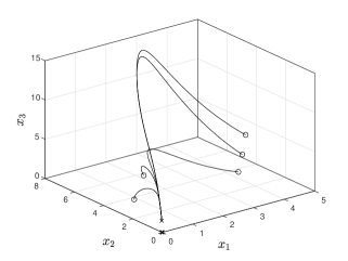
Figure 3: Trajectories of (VI-A) from five initial conditions marked by circles. Equilibrium points are marked by a cross.

VII Conclusion

We derived a sufficient condition for $k$-contraction of a generalized Lurie system, that is, the feedback connection of nonlinear dynamical system and a nonlinear feedback function. Such systems typically have more than a single equilibrium and are thus not $1$-contracting w.r.t. any norm. Nevertheless, if they are $2$-contracting then every bounded solution converges to an equilibrium (which is not necessarily unique) and establishing such a global property is important in many applications. For example, in a neural network model of an associative memory every stored memory pattern corresponds to an equilibrium, and $2$-contraction implies that for any initial condition the solution will indeed converge to some stored pattern.

Topics for further research include the following. First, a given nonlinear system can often be represented as a generalized Lurie system in several ways. An interesting question is how to find the “best” possible representation? Second, our results only consider $k$-contraction w.r.t. (scaled) $L_{2}$ norms and it may be of interest to analyze $k$-contraction w.r.t. other norms. Third, Theorem 2 provides a sufficient condition for $k$-contraction that uses the singular values of the connection matrices $W_{1}$ and $W_{2}$ in the networked system (27). In other words, it is based on the spectral properties of the connection graphs (see also Remark 6). An interesting research direction is to further develop this into a graph-theoretic approach to $k$-contraction.

References

• [1] Z. Aminzare and E. D. Sontag, “Contraction methods for nonlinear systems: A brief introduction and some open problems,” in Proc. 53rd IEEE Conf. on Decision and Control, Los Angeles, CA, 2014, pp. 3835–3847.
• [2] V. Andrieu and S. Tarbouriech, “LMI conditions for contraction and synchronization,” IFAC-PapersOnLine, vol. 52, no. 16, pp. 616–621, 2019, 11th IFAC Symposium on Nonlinear Control Systems (NOLCOS 2019).
• [3] D. Angeli, J. E. Ferrell, and E. D. Sontag, “Detection of multistability, bifurcations, and hysteresis in a large class of biological positive-feedback systems,” Proceedings of the National Academy of Sciences, vol. 101, no. 7, pp. 1822–1827, 2004.
• [4] D. Angeli, D. Martini, G. Innocenti, and A. Tesi, “A small-gain theorem for 2-contraction of nonlinear interconnected systems,” 2023. [Online]. Available: https://arxiv.org/abs/2305.03211
• [5] E. M. Aylward, P. A. Parrilo, and J.-J. E. Slotine, “Stability and robustness analysis of nonlinear systems via contraction metrics and SOS programming,” Automatica, vol. 44, no. 8, pp. 2163–2170, 2008.
• [6] E. Bar-Shalom, O. Dalin, and M. Margaliot, “Compound matrices in systems and control theory: a tutorial,” Math. Control Signals Systems, 2023.
• [7] N. Boffi, S. Tu, N. Matni, J.-J. Slotine, and V. Sindhwani, “Learning stability certificates from data,” in Proceedings of the 2020 Conference on Robot Learning, ser. Proceedings of Machine Learning Research, vol. 155, 2021, pp. 1341–1350.
• [8] N. M. Boffi and J.-J. E. Slotine, “Implicit regularization and momentum algorithms in nonlinearly parameterized adaptive control and prediction,” Neural Computation, vol. 33, no. 3, pp. 590–673, 2021.
• [9] F. Bullo, Contraction Theory for Dynamical Systems.   Kindle Direct Publishing, 2022. [Online]. Available: http://motion.me.ucsb.edu/book-ctds
• [10] V. Centorrino, A. Gokhale, A. Davydov, G. Russo, and F. Bullo, “Euclidean contractivity of neural networks with symmetric weights,” IEEE Control Systems Letters, vol. 7, pp. 1724–1729, 2023.
• [11] C.-Y. Cheng, K.-H. Lin, and C.-W. Shin, “Multistability in recurrent neural networks,” SIAM J. Applied Math., vol. 66, no. 4, pp. 1301–1320, 2006.
• [12] S.-J. Chung and J.-J. E. Slotine, “Cooperative robot control and concurrent synchronization of Lagrangian systems,” IEEE Trans. Robot., vol. 25, no. 3, pp. 686–700, 2009.
• [13] M. A. Cohen and S. Grossberg, “Absolute stability of global pattern formation and parallel memory storage by competitive neural networks,” IEEE Trans. Systems, Man, and Cybernetics, vol. SMC-13, no. 5, pp. 815–826, 1983.
• [14] O. Dalin, R. Ofir, E. B. Shalom, A. Ovseevich, F. Bullo, and M. Margaliot, “Verifying $k$-contraction without computing $k$-compounds,” 2022, submitted. [Online]. Available: https://arxiv.org/abs/2209.01046
• [15] A. Davydov, S. Jafarpour, and F. Bullo, “Non-Euclidean contraction theory for robust nonlinear stability,” IEEE Trans. Automat. Control, vol. 67, no. 12, pp. 6667–6681, 2022.
• [16] A. Fradkov, “Early ideas of the absolute stability theory,” in 2020 European Control Conference (ECC), 2020, pp. 762–768.
• [17] M. Giaccagli, V. Andrieu, S. Tarbouriech, and D. Astolfi, “Infinite gain margin, contraction and optimality: an LMI-based design,” Euro. J. Control, p. 100685, 2022.
• [18] R. A. Horn and C. R. Johnson, Topics in Matrix Analysis.   Cambridge University Press, 1991.
• [19] S. Jafarpour, A. Davydov, A. Proskurnikov, and F. Bullo, “Robust implicit networks via non-Euclidean contractions,” in Advances in Neural Information Processing Systems, M. Ranzato, A. Beygelzimer, Y. Dauphin, P. Liang, and J. W. Vaughan, Eds., vol. 34.   Curran Associates, Inc., 2021, pp. 9857–9868.
• [20] H. K. Khalil, Nonlinear Systems, 3rd ed.   Upper Saddle River, NJ: Prentice-Hall, 2002.
• [21] A. Lakshmanan, A. Gahlawat, and N. Hovakimyan, “Safe feedback motion planning: A contraction theory and $\mathcal{L}_{1}$-adaptive control based approach,” in Proc. 59th IEEE Conf. on Decision and Control, 2020, pp. 1578–1583.
• [22] G. Leonov, I. M. Burkin, and A. I. Shepeljavyi, Frequency Methods in Oscillation Theory.   Springer, 1996.
• [23] M. Y. Li and J. S. Muldowney, “On R. A. Smith’s autonomous convergence theorem,” Rocky Mountain J. Math., vol. 25, no. 1, pp. 365–378, 1995.
• [24] M. R. Liberzon, “Lur’e problem of absolute stability - a historical essay,” IFAC Proc. Volumes, vol. 34, no. 6, pp. 25–28, 2001, 5th IFAC Symposium on Nonlinear Control Systems 2001, St Petersburg, Russia, 4-6 July 2001.
• [25] W. Lohmiller and J.-J. E. Slotine, “On contraction analysis for non-linear systems,” Automatica, vol. 34, pp. 683–696, 1998.
• [26] K. A. Lurie, “Some recollections about Anatolii Isakovich Lurie,” IFAC Proc. Volumes, vol. 34, no. 6, pp. 35–38, 2001, 5th IFAC Symp. Nonlinear Control Systems, St. Petersburg, Russia.
• [27] I. R. Manchester and J.-J. E. Slotine, “Control contraction metrics: Convex and intrinsic criteria for nonlinear feedback design,” IEEE Trans. Automat. Control, vol. 62, no. 6, pp. 3046–3053, 2017.
• [28] ——, “Combination properties of weakly contracting systems,” 2015. [Online]. Available: https://arxiv.org/abs/1408.5174
• [29] M. Margaliot, E. D. Sontag, and T. Tuller, “Entrainment to periodic initiation and transition rates in a computational model for gene translation,” PLoS ONE, vol. 9, no. 5, p. e96039, 2014.
• [30] M. Margaliot, “Stability analysis of switched systems using variational principles: An introduction,” Automatica, vol. 42, no. 12, pp. 2059–2077, 2006.
• [31] M. Margaliot, E. D. Sontag, and T. Tuller, “Contraction after small transients,” Automatica, vol. 67, pp. 178–184, 2016.
• [32] J. S. Muldowney, “Compound matrices and ordinary differential equations,” Rocky Mountain J. Math., vol. 20, no. 4, pp. 857–872, 1990.
• [33] H. D. Nguyen, T. L. Vu, J.-J. Slotine, and K. Turitsyn, “Contraction analysis of nonlinear DAE systems,” IEEE Trans. Automat. Control, vol. 66, no. 1, 2021.
• [34] R. Ofir, M. Margaliot, Y. Levron, and J.-J. Slotine, “Serial interconnections of 1-contracting and 2-contracting systems,” in Proc. 60th IEEE Conf. on Decision and Control, 2021, pp. 3906–3911.
• [35] ——, “A sufficient condition for $k$-contraction of the series connection of two systems,” IEEE Trans. Automat. Control, vol. 67, no. 9, pp. 4994–5001, 2022.
• [36] R. Ofir, A. Ovseevich, and M. Margaliot, “Contraction and k-contraction in Lurie systems with applications to networked systems,” Automatica, 2023, to appear. [Online]. Available: https://arxiv.org/abs/2212.13440
• [37] Q.-C. Pham and J.-J. Slotine, “Stable concurrent synchronization in dynamic system networks,” Neural Networks, vol. 20, no. 1, pp. 62–77, 2007.
• [38] A. V. Proskurnikov, A. Davydov, and F. Bullo, “The Yakubovich S-Lemma revisited: Stability and contractivity in non-Euclidean norms,” SIAM J. Control Optim., vol. 61, no. 4, pp. 1955–1978, 2023.
• [39] H. Qiao, J. Peng, and Z.-B. Xu, “Nonlinear measures: a new approach to exponential stability analysis for Hopfield-type neural networks,” IEEE Trans. Neural Networks, vol. 12, no. 2, pp. 360–370, 2001.
• [40] M. Revay, R. Wang, and I. R. Manchester, “Recurrent equilibrium networks: Flexible dynamic models with guaranteed stability and robustness,” IEEE Trans. Automat. Control, pp. 1–16, 2023.
• [41] G. Russo, M. di Bernardo, and E. D. Sontag, “Global entrainment of transcriptional systems to periodic inputs,” PLOS Computational Biology, vol. 6, p. e1000739, 2010.
• [42] G. Russo, M. di Bernardo, and E. Sontag, “A contraction approach to the hierarchical analysis and design of networked systems,” IEEE Trans. Automat. Control, vol. 58, no. 5, pp. 1328–1331, 2013.
• [43] G. Russo, M. di Bernardo, and J. J. Slotine, “Contraction theory for systems biology,” in Design and Analysis of Biomolecular Circuits: Engineering Approaches to Systems and Synthetic Biology, H. Koeppl, G. Setti, M. di Bernardo, and D. Densmore, Eds.   New York, NY: Springer, 2011, pp. 93–114.
• [44] S. Singh, B. Landry, A. Majumdar, J.-J. Slotine, and M. Pavone, “Robust feedback motion planning via contraction theory,” Int. J. Robotics Research, 2023.
• [45] H. L. Smith, Monotone Dynamical Systems: An Introduction to the Theory of Competitive and Cooperative Systems, ser. Mathematical Surveys and Monographs.   Providence, RI: Amer. Math. Soc., 1995, vol. 41.
• [46] D. Sun, S. Jha, and C. Fan, “Learning certified control using contraction metric,” in Proceedings of the 2020 Conference on Robot Learning, ser. Proceedings of Machine Learning Research, vol. 155, 2021, pp. 1519–1539.
• [47] H. Tsukamoto, S.-J. Chung, and J.-J. E. Slotine, “Neural stochastic contraction metrics for learning-based control and estimation,” IEEE Control Systems Letters, vol. 5, no. 5, pp. 1825–1830, 2021.
• [48] M. Vidyasagar, Nonlinear Systems Analysis.   SIAM, 2002.
• [49] W. Wang and J. J. E. Slotine, “On partial contraction analysis for coupled nonlinear oscillators,” Biological Cybernetics, vol. 92, no. 1, 2005.
• [50] P. M. Wensing and J.-J. Slotine, “Beyond convexity—contraction and global convergence of gradient descent,” PLOS ONE, vol. 15, no. 8, pp. 1–29, 08 2020.
• [51] C. Wu, I. Kanevskiy, and M. Margaliot, “$k$-contraction: theory and applications,” Automatica, vol. 136, p. 110048, 2022.
• [52] C. Wu, R. Pines, M. Margaliot, and J.-J. Slotine, “Generalization of the multiplicative and additive compounds of square matrices and contraction theory in the Hausdorff dimension,” IEEE Trans. Automat. Control, vol. 67, no. 9, pp. 4629–4644, 2022.