A Fast Optimization View: Reformulating Single Layer Attention
in LLM Based on Tensor and SVM Trick, and Solving It in Matrix Multiplication Time

Large language models have played a pivotal role in revolutionizing various facets of our daily existence. Serving as the cornerstone of virtual assistants, they have seamlessly streamlined information retrieval and task automation. Spanning domains from healthcare to education, these models have made an enduring impact, elevating productivity, decision-making processes, and accessibility, thereby influencing and, to a certain extent, reshaping the lifestyles of people.

Solving attention regression is a fundamental task in optimizing LLMs. In this work, we focus on giving a provable guarantee for the one-layer attention network objective function

$$L(X,Y)=\sum_{j_{0}=1}^{n}\sum_{i_{0}=1}^{d}(\langle\langle\exp(\operatorname{\mathsf{A}}_{j_{0}}x),{\bf 1}_{n}\rangle^{-1}\exp(\operatorname{\mathsf{A}}_{j_{0}}x),A_{3}Y_{*,i_{0}}\rangle-b_{j_{0},i_{0}})^{2}$$

Here $\mathsf{A}\in\mathbb{R}^{n^{2}\times d^{2}}$ is Kronecker product between $A_{1}\in\mathbb{R}^{n\times d}$ and $A_{2}\in\mathbb{R}^{n\times d}$. $A_{3}$ is a matrix in $\mathbb{R}^{n\times d}$, $\mathsf{A}_{j_{0}}\in\mathbb{R}^{n\times d^{2}}$ is the $j_{0}$-th block of $\mathsf{A}$. The $X,Y\in\mathbb{R}^{d\times d}$ are variables we want to learn. $B\in\mathbb{R}^{n\times d}$ and $b_{j_{0},i_{0}}\in\mathbb{R}$ is one entry at $j_{0}$-th row and $i_{0}$-th column of $B$, $Y_{*,i_{0}}\in\mathbb{R}^{d}$ is the $i_{0}$-column vector of $Y$, and $x\in\mathbb{R}^{d^{2}}$ is the vectorization of $X$.

In a multi-layer LLM network, the matrix $B\in\mathbb{R}^{n\times d}$ can be viewed as the output of a layer, and $A_{1}=A_{2}=A_{3}\in\mathbb{R}^{n\times d}$ can be viewed as the input of a layer. The matrix version of $x$ can be viewed as $QK^{\top}$ and $Y$ can be viewed as $V$. We provide an iterative greedy algorithm to train loss function $L(X,Y)$ up $\epsilon$ that runs in $\widetilde{O}(({\cal T}_{\mathrm{mat}}(n,n,d)+{\cal T}_{\mathrm{mat}}(n,d,d)+d^{2\omega})\log(1/\epsilon))$ time. Here ${\cal T}_{\mathrm{mat}}(a,b,c)$ denotes the time of multiplying $a\times b$ matrix another $b\times c$ matrix, and $\omega\approx 2.37$ denotes the exponent of matrix multiplication.

1 Introduction

Large language models (LLMs) like GPT-1 [149], BERT [49], GPT-2 [154], GPT-3 [24], ChatGPT [35], GPT-4 [134], OPT [209], Llama [174], and Llama 2 [176] have demonstrated impressive capabilities in natural language processing (NLP). These models understand and generate complex language, enabling a wide range of applications such as sentiment analysis [200], language translation [1], question answering [23], and text summarization [137]. Despite their high-quality performance, there remains untapped potential in optimizing and training these massive models, making it a challenging endeavor in the present day.

The primary technical foundation supporting the capabilities of LLMs is the attention matrix [149, 179, 24, 49]. The central concept of attention is to learn representations that emphasize the most relevant parts of the input. To be more specific, the attention mechanism compares the query vectors (the output tokens) with the key vectors (the input tokens). The attention weights are then determined based on the similarity of this comparison, indicating the relative importance of each input token. These attention weights are used to compute weighted averages of the value vectors, resulting in the output representation. By leveraging attention, LLMs acquire the ability to focus on the crucial aspects of the input, allowing them to gather pertinent information more efficiently and precisely. This capability enables LLMs to process longer texts effectively and comprehend intricate semantic relationships. Notably, the self-attention mechanism enables LLMs to establish connections between various segments of the input sequence, enhancing their contextual understanding.

We start with defining the general Attention forward layer,

Definition 1.1 ($\ell$-th layer forward computation).

Let ${\bf 1}_{n}$ be the $n$-dimensional vector whose entries are all $1$. Let $\operatorname{diag}:\mathbb{R}^{n}\to\mathbb{R}^{n\times n}$ be a function: each entry of the vector in $\mathbb{R}^{n}$ is mapped to the diagonal entry of the matrix in $\mathbb{R}^{n\times n}$ and other entries of this matrix are all $0$’s. Given weights $Q,K,V\in\mathbb{R}^{d\times d}$, let $X_{\ell}\in\mathbb{R}^{n\times d}$ denote the $\ell$-th layer input and $X_{\ell+1}\in\mathbb{R}^{n\times d}$

$$X_{\ell+1}\leftarrow D^{-1}\exp(X_{\ell}QK^{\top}X_{\ell}^{\top})X_{\ell}V$$

where $D:=\operatorname{diag}(\exp(X_{\ell}QK^{\top}X_{\ell}^{\top}){\bf 1}_{n})$

Mathematically, a general optimization with respect to attention computation is defined as:

Definition 1.2 (Attention optimization).

Let $A_{1},A_{2},A_{3},B\in\mathbb{R}^{n\times d}$ and $X,Y\in\mathbb{R}^{d\times d}$. The attention computation is defined as:

$$\min_{X,Y\in\mathbb{R}^{d\times d}}\|D(X)^{-1}\exp(A_{1}XA_{2}^{\top})A_{3}Y-B\|_{F}^{2},$$

where $D(X)\in\mathbb{R}^{n\times n}$ is $D(X):=\operatorname{diag}(\exp(A_{1}XA_{2}^{\top}){\bf 1}_{n})$.

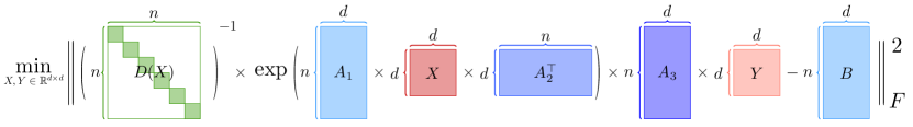
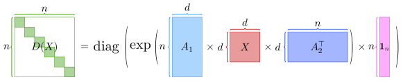
Figure 1: The visualization of the attention optimization (see Definition 1.2). Let $A_{1},A_{2},A_{3},B\in\mathbb{R}^{n\times d}$ and $X,Y\in\mathbb{R}^{d\times d}$. We first get $\exp(A_{1}XA_{2}^{\top})\in\mathbb{R}^{n\times n}$ by multiplying $A_{1}$, $X$, and $A_{2}^{\top}$. Then, we have $D(X)\in\mathbb{R}^{n\times n}$ by computing $\operatorname{diag}(\exp(A_{1}XA_{2}^{\top}){\bf 1}_{n})$. After that, we multiply $D(X)^{-1}$, $\exp(A_{1}XA_{2}^{\top})$, $A_{3}$, and $Y$ and subtract $B$ from their product. Finally, we compute the minimum of the Frobenius norm of their difference. The blue rectangles represent the $n\times d$ matrices, the purple rectangle represents the $n$-dimensioal vector, the red squares represent the $d\times d$ matrices, and the green squares represent the $n\times n$ diagonal matrices.

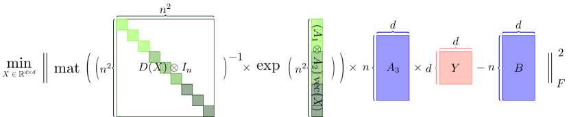
Figure 2: The visualization of a variation of Definition 1.2. Let $A_{1},A_{2},A_{3},B\in\mathbb{R}^{n\times d}$, $X\in\mathbb{R}^{d\times d}$, $D(X)\in\mathbb{R}^{n\times n}$ (see Figure 1 and Definition 1.2), and $\operatorname{\mathsf{A}}=A_{1}\otimes A_{2}\in\mathbb{R}^{n^{2}\times d^{2}}$. $\mathrm{mat}:\mathbb{R}^{n^{2}}\to\mathbb{R}^{n\times n}$ is defined by $X_{i,j}=\mathrm{mat}(x)_{i,j}:=x_{(i-1)\cdot n+j}$, and $\operatorname{vec}=\mathrm{mat}^{-1}$. We first get that $(D(X)\otimes I_{n})^{-1}\in\mathbb{R}^{n^{2}\times n^{2}}$ and multiply $\operatorname{\mathsf{A}}$ with $\operatorname{vec}(X)$. Then, we multiply $(D(X)\otimes I_{n})^{-1}\in\mathbb{R}^{n^{2}\times n^{2}}$ with $\operatorname{\mathsf{A}}\cdot\operatorname{vec}(X)\in\mathbb{R}^{n^{2}}$, which gives us a vector in $\mathbb{R}^{n^{2}}$. We use $\mathrm{mat}$ to transform that into a matrix in $\mathbb{R}^{n\times n}$. After that, we multiply this matrix with $A_{3}Y\in\mathbb{R}^{n\times d}$. Finally, we compute the minimum of the Frobenius norm of $\mathrm{mat}((D(X)\otimes I_{n})^{-1}\cdot\exp(\operatorname{\mathsf{A}}\operatorname{vec}(X)))A_{3}Y-B$. In this figure, we give an example when $n=3$: in the matrix $D(X)\otimes I_{n}$, the three light green squares (and their nearby white area) make up the first chunk, the three middle green squares (and their nearby white area) make up the second chunk, and the three dark green squares (and their nearby white area) make up the third chunk. The blue rectangles represent the matrices in $\mathbb{R}^{n\times d}$. The red rectangle represents the matrix in $\mathbb{R}^{d\times d}$.

Here $X=QK^{\top},Y=V$ are the weights we want to learn, and $A_{1},A_{2},A_{3}$ are the input of a layer $X_{\ell}$, and the $B$ are the output layer $X_{\ell+1}$. Attention computation has been analyzed in many recent works [203, 11, 29, 75, 57, 171, 175, 139, 125, 208, 140, 159], but none of them give a complete analysis of the full version of the attention computation problem. They all simplify this problem by different strategies (see details in Table 1).

However, simplifying this problem may lead to a significant decrease in the model performance, which may require extra model training or fine-tuning. This results in deployment obstacles.

In this paper, our focus is on optimizing the attention mechanism. Our goal is to present a complete, un-simplified analysis of the attention problem defined in Definition 1.2, a task that, to the best of our knowledge, has not been done before. We provide a provable guarantee for optimizing the attention function in the case of a single-layer attention network. Our motivation stems from the critical role of the attention optimization problem in the functionality of LLMs, and we firmly believe that our theoretical analysis will significantly influence the development of LLMs.

As [11], they show that one step forward computation of attention can be done in $o(n^{2})$ time without formulating the $n\times n$ matrix. However, it is still an open problem about how fast we optimize the loss function via the iterative method.

How fast can we optimize the training process of attention matrix (See Definition 1.2)?

In this study, we make progress towards this fundamental question.

To establish the correctness of our algorithm, we conduct a comprehensive analysis of the positive semi-definite (PSD) property and the Lipschitz continuity of the Hessian matrix constructed from the attention matrix. These two properties provide the necessary assurance for employing TensorSRHT and Newton’s method, ensuring both fast computation and convergence, respectively.

Now, we will present our main result as follows.

Theorem 1.3 (Informal version of our main theorem).

Let $A_{1},A_{2},A_{2}\in\mathbb{R}^{n\times d}$. There is an algorithm that runs in $\widetilde{O}({\cal T}_{\mathrm{mat}}(n,d,n)+{\cal T}_{\mathrm{mat}}(n,d,d)+d^{2\omega})\log(1/\epsilon)$ solves to the attention problem up to $\epsilon$ accuracy with probability $1-1/\operatorname{poly}(n)$. Here $\omega\approx 2.37$.

Here $\omega$ denotes the exponent of matrix multiplication [182, 105, 15, 62, 106, 189], ${\cal T}_{\mathrm{mat}}(a,b,c)$ denotes the time of multiplying an $a\times b$ size matrix with another $b\times c$ size matrix, and ${\cal T}_{\mathrm{mat}}(n,n,n)=n^{\omega}$. See more details of matrix multiplication notation in Section 4.7.

Relationship with the Softmax Regression Problem

Moreover, the attention weight can be viewed as the output of a softmax regression model, which is defined as follows:

Definition 1.4 (Single softmax regression [55] and multiple softmax regression [72]).

Given a matrix $A\in\mathbb{R}^{n\times d}$ and a vector $c\in\mathbb{R}^{n}$, the single softmax regression problem is defined as

$${\bf Part~{}1.}\min_{x\in\mathbb{R}^{d}}\|\langle\exp(Ax),{\bf 1}_{n}\rangle^{-1}\exp(Ax)-c\|_{2}^{2}.$$

Let $D(X)\in\mathbb{R}^{n\times n}$ be defined as in Definition 1.2. Given $A_{1},A_{2}\in\mathbb{R}^{n\times d}$ and $X\in\mathbb{R}^{d\times d}$

$${\bf Part~{}2.}\min_{X\in\mathbb{R}^{d\times d}}\|D(X)^{-1}\exp(A_{1}XA_{2}^{\top})-C\|_{F}^{2}$$

On the one hand, due to the observation in [72, 73], the equation in Part 1 of Definition 1.4 can be viewed as one row of the equation in Part 2 of Definition 1.4.

On the other hand, due to the well-known tensor trick (see [58, 52] as an example), the Part 2 equation Definition 1.4 is equivalent to

$$\min_{X\in\mathbb{R}^{d\times d}}\|(D(X)\otimes I_{n})^{-1}\exp(\operatorname{\mathsf{A}}\operatorname{vec}(X))-\operatorname{vec}(C)\|_{2}^{2},$$ (1)

which can be a slightly more complicated version of the Part 1 equation in Definition 1.4. In particular, instead of one re-scaling factor, we will have $n$ rescaling factor. We split $\exp(\operatorname{\mathsf{A}}\operatorname{vec}(X))\in\mathbb{R}^{n^{2}}$ into $n$ chunks, and each chunk has size $n$. For each chunk, we use the same rescaling factor.

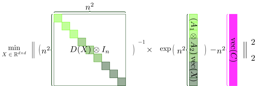
Figure 3: The visualization of Eq. (1). Let $A_{1},A_{2}\in\mathbb{R}^{n\times d}$, $X\in\mathbb{R}^{d\times d}$, $C,D(X)\in\mathbb{R}^{n\times n}$ (see Figure 1 and Definition 1.2), and $\operatorname{\mathsf{A}}=A_{1}\otimes A_{2}\in\mathbb{R}^{n^{2}\times d^{2}}$. We first get that $(D(X)\otimes I_{n})^{-1}\in\mathbb{R}^{n^{2}\times n^{2}}$ and multiply $\operatorname{\mathsf{A}}$ with $\operatorname{vec}(X)$. Then, we multiply $(D(X)\otimes I_{n})^{-1}\in\mathbb{R}^{n^{2}\times n^{2}}$ with $\operatorname{\mathsf{A}}\cdot\operatorname{vec}(X)\in\mathbb{R}^{n^{2}}$. After that, we compute $c=\operatorname{vec}(C)\in\mathbb{R}^{n^{2}}$ and subtract it from $(D(X)\otimes I_{n})^{-1}\exp(\operatorname{\mathsf{A}}\cdot\operatorname{vec}(X))$. Finally, we compute the minimum of the $\ell_{2}$ norm of $(D(X)\otimes I_{n})^{-1}\exp(\operatorname{\mathsf{A}}\cdot\operatorname{vec}(X))-c$. In this figure, we give an example when $n=3$: in the matrix $D(X)\otimes I_{n}$, the three light green squares (and their nearby white area) make up the first chunk, the three middle green squares (and their nearby white area) make up the second chunk, and the three dark green squares (and their nearby white area) make up the third chunk. The purple rectangle represents $c=\operatorname{vec}(C)\in\mathbb{R}^{n^{2}}$.

Note that the multiple softmax regression problem is a simplified version of what we study in Definition 1.2. We believe that our work can also support the study of softmax regression.

Relatinship with Support Vector Machines (SVM)

The usual SVM [91, 37, 77, 175] objective function in optimization can be viewed as a product of a summation of a batch of inner product. Inspired by that, we can define $n$ functions $f(x)_{j_{0}}\in\mathbb{R}^{n}$ for each $j_{0}\in[n]$ and $d$ functions $h(Y)_{i_{0}}\in\mathbb{R}^{n}$. Here $x$ is the vectorization of $X$ and $y$ is the vectorization of $Y$. Then the objective function in Definition 1.2 $\|D(X)^{-1}\exp(A_{1}XA_{2}^{\top})A_{3}Y-B\|_{F}^{2}$ can be turned into

$$\sum_{j_{0}=1}^{n}\sum_{i_{0}=1}^{d}(\langle f(x)_{j_{0}},h(Y)_{i_{0}}\rangle-b_{j_{0},i_{0}})^{2}$$ (2)

where $b_{j_{0},i_{0}}$ is the entry of matrix $B\in\mathbb{R}^{n\times d}$. We call this formulation SVM-inspired formulation.

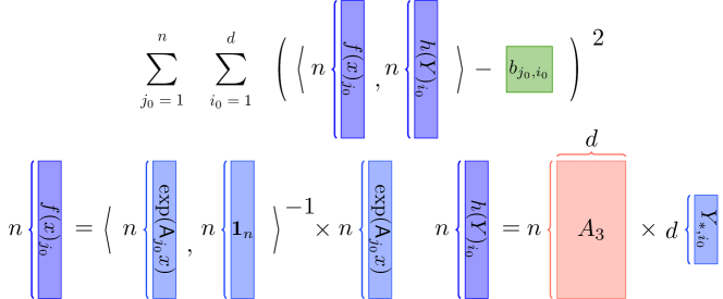
Figure 4: The visualization of Eq. (2). Let $A_{1},A_{2},A_{3},B\in\mathbb{R}^{n\times d}$ and $X,Y\in\mathbb{R}^{d\times d}$. We have $\operatorname{\mathsf{A}}=A_{1}\otimes A_{2}\in\mathbb{R}^{n^{2}\times d^{2}}$ and $\operatorname{\mathsf{A}}_{j_{0}}\in\mathbb{R}^{n\times d^{2}}$ is the $j_{0}$-th block of $\operatorname{\mathsf{A}}$. $x=\operatorname{vec}(X)\in\mathbb{R}^{d^{2}}$. First, we use the definition of $f(x)_{j_{0}}\in\mathbb{R}^{n}$ (see Definition 4.10) and $h(Y)_{i_{0}}\in\mathbb{R}^{n}$ (see Definition 4.11) to compute them. Then, we find their inner produce and subtract the entry of $B$ at $j_{0}$-th row and $i_{0}$-column from the inner produce. Finally, we compute the square of this difference and add all of them from $i_{0}=1$ to $i_{0}=d$ and from $j_{0}=1$ to $j_{0}=n$. In this figure, we use blue rectangles to represent vectors, where the dark blue represents $f(x)_{j_{0}}$ and $h(Y)_{i_{0}}$, and the light blue represents the terms used to compute $f(x)_{j_{0}}$ and $h(Y)_{i_{0}}$. The green square represents the scalar. The red rectangle represents the matrix.

Roadmap

In Section 2, we introduce related research work. In Section 3, we provide an overview of the techniques we will use throughout the rest of the paper. In Section 4, we present the basic notations we use, some mathematical facts, and helpful definitions that support the following proof. In Section 5, we compute the gradients of the helpful functions defined earlier. In Section 6, we define the Hessian for further discussion. In Section 7, we compute the Hessian matrix with respect to $X$. In Section 8, we demonstrate that the Hessian for $X$ is Lipschitz. In Section 9, we show that the Hessian matrix with respect to $X$ is positive semidefinite (PSD). In Section 10, we compute the Hessian matrix with respect to $Y$ and show that it is Lipschitz and positive semidefinite (PSD). In Section 11, we compute the Hessian matrix with respect to both $X$ and $Y$. In Section 12, we demonstrate that the Hessian matrix with respect to both $X$ and $Y$ is Lipschitz. In Section 13, we introduce some tensor sketch techniques to obtain fast approximations of the Hessian. In Section 14, we introduce the Newton step.

2 Related Work

Attention

[18] represents one of the earliest works that employed attention in NLP. They assumed that a fixed-length vector could enhance the performance of the encoder-decoder design by incorporating an attention mechanism. This mechanism allows the decoder to focus on relevant words in the source sentence while generating translations. Consequently, this approach significantly improves the performance of machine translation models compared to those without an attention mechanism. Subsequently, [113] explained two variants of attention: local attention, which considers a subset of source words at a time, and global attention, which attends to all source words.

Attention finds extensive applications across various domains. In image captioning, [192] utilizes attention matrices to align specific parts of an image with words in a caption. In the context of the Transformer model [179], attention matrices capture differences between words in a sentence. In the realm of graph neural networks, [177] investigates these neural network architectures designed for graph-structured data, computing attention matrices between each node and its neighbors.

On the theoretical side, after the emergence of LLMs, there has been a substantial body of work dedicated to studying attention computation [57, 11, 203, 40, 118, 29, 99]. Notably, recent research by [203, 40, 99] employs Locality Sensitive Hashing (LSH) techniques to approximate attention mechanisms. In particular, [203] introduces $\mathsf{KDEformer}$, an efficient algorithm for approximating dot-product attention. This algorithm provides provable spectral norm bounds and outperforms various pre-trained models. Additionally, current research explores both static and dynamic approaches to calculating attention, as evidenced by the works of [29] and [11]. Furthermore, [118] delves into the regularization of hyperbolic regression problems, which involve functions like $\exp$, $\sinh$, and $\cosh$. Lastly, [57] proposes randomized and deterministic algorithms for reducing the dimensionality of attention matrices in LLMs, achieving high accuracy while significantly reducing feature dimensions.

Additionally, numerous studies have attempted to analyze theoretical attention from the perspectives of optimization and convergence [111, 69, 172, 205]. [111] investigated how transformers acquire knowledge about word co-occurrence patterns. [69] focused on studying regression problems inspired by neural networks that employ exponential activation functions. [172] analyzed why models occasionally prioritize significant words and explained how the attention mechanism evolves during the training process. [205] demonstrated that the presence of a heavy-tailed noise distribution contributes to the bad performance of stochastic gradient descent (SGD) compared to adaptive methods.

Theoretical LLMs

There are numerous amount of works focusing on the theoretical aspects of LLMs. In [155], the syntactic representations of the attention matrix and the individual word embeddings are presented, together with the mathematical justification of elucidating the geometrical properties of these representations. [84] introduces a structural probe that analyzes, under the linear transformation of a word representation space of a neural network, whether or not syntax trees are embedded.

[39, 110, 151, 100] study the optimization of LLMs. [39] proposes a new algorithm called ZO-BCD. It has favorable overall query complexity and a smaller computational complexity in each iteration. [110] creates a simple scalable second-order optimizer, called Sophia. In different parts of the parameter, Sophia adapts to the curvature. This may be strongly heterogeneous for language modeling tasks. The bound of the running time does not rely on the condition number of the loss.

Other theoretical LLM papers study the knowledge and skills of LLMs. [188] analyzes distinct “skill” neurons, which are regarded as robust indicators of downstream tasks when employing the process of soft prompt-tuning, as discussed in [108], for language models. [50] find a positive relationship between the activation of these neurons and the expression of their corresponding facts, through analyzing BERT. Simultaneously, [32] employs a fully unsupervised approach to extract latent knowledge from a language model’s internal activations. In addition, [79] and [124] show that in the feed-forward layers of pre-trained models, language models localize knowledge. [194] explores the feasibility of selecting a specific subset of layers for modification and determining the optimal location for integrating a classifier. [123] demonstrate that large trained transformers exhibit sparsity in their feedforward activations. Zero-th order algorithm for training LLM has been analyzed [125, 54, 204].

LLMs Application and Evaluation

Recently, there has been much interest in developing LLM-based systems for conversational AI and task-oriented dialogue, like Google’s Meena chatbot [148], Microsoft 365 Copilot [161], Adobe firefly, Adobe Photoshop, GPT series [149, 154, 24, 35, 134], and BERT [49].

Moreover, LLM evaluation is also a popular research area. Within the field of NLP, LLMs are evaluated based on natural language understanding [20, 102, 103, 45], reasoning [23, 187, 193], natural language generation [183, 147, 137, 36, 47], and multilingual tasks [10, 5, 112, 199]. Robustness [109, 181, 207], ethics [48], biases [65], and trustworthiness [80] are also important aspects. More specifically, the abilities of LLMs in social science [51, 66, 131], mathematics [12, 53, 184, 19], science [42, 67], engineering [19, 122, 138, 160], and medical applications [38, 87] are evaluated.

Sketching

Sketching is a powerful tool that is used to accelerate the performance of machine learning algorithms and optimization processes. The fundamental concept of sketching is to partition a large input matrix into a significantly smaller sketching matrix but still preserve the main characteristics of the original matrix. Therefore, the algorithms may work with the smaller matrix instead of the huge original, which leads to a substantial reduction in processing time. Many previous works have studied sketching, proposed sketching algorithms, and supported these algorithms with robust theoretical guarantees. For example, the Johnson-Lindenstrauss lemma is proposed by [89]: it shows that under a certain high-dimensional space, projecting points to a lower-dimensional subspace may preserve the pairwise distances between these points. This mathematical property becomes the foundation of the development of faster algorithms for tasks such as nearest neighbor search. In addition, as explained in [2], the Fast Johnson-Lindenstrauss Transform (FJLT) introduces a specific family of structured random projections that can be applied to a matrix in input sparsity time.

More recently, sketching has been applied to many numerical linear algebra tasks, such as linear regression [46, 133], dynamic kernel estimation [143], submodular maximization [144], matrix sensing [145], gradient-based algorithm [195], clustering [59, 64], convex programming [167, 146, 93, 90, 117], online optimization problems [150], training neural networks [173, 197, 169, 70, 25], reinforcement learning [191, 196], tensor decomposition [165, 60], relational database [141], low-rank approximation [30, 128, 126, 8, 164], distributed problems [31, 190], weighted low rank approximation [152, 76, 168], CP decomposition [129], regression inspired by softmax [118, 74, 162, 55], matrix sensing [145], and Kronecker product regression [153].

Second-order Method

Second-order method have been used for solving many convex optimization and non-convex optimization problems, such as linear programming [41, 26, 93, 167, 71, 83], empirical risk minimization [117, 146], support vector machines [77], cutting plan method [116, 90], semi-definite programming [88, 81, 71, 170], hyperbolic programming/polynomials [61, 211], streaming algorithm [119, 27, 170], federated learning [28].

Convergence and Deep Neural Network Optimization

Many works focus on analyzing optimization, convergence guarantees, and training improvement. [107] shows that stochastic gradient descent optimizes over-parameterized neural networks on structured data, while [63] demonstrates that gradient descent optimizes over-parameterized neural networks. In [16], a convergence theory for over-parameterized deep neural networks via gradient descent is developed. [17] analyzes the convergence rate of training recurrent neural networks. [3] provides a fine-grained analysis of optimization and generalization for over-parameterized two-layer neural networks. [4] studies exact computation with an infinitely wide neural network. [33] proposes a Gram-Gauss-Newton method for optimizing over-parameterized neural networks. [201] improves the analysis of the global convergence of stochastic gradient descent when training deep neural networks, requiring a milder over-parameterization compared to prior research. Other research, such as [135, 96, 206], focuses on optimization and generalization, while [69, 118] emphasize the convergence rate and stability. Works like [25, 173, 9, 127, 202] concentrate on specialized optimization algorithms and techniques for training neural networks, and [115, 82] concentrate on leveraging neural network structure.

Algorithmic Regularization

There is a significant body of research exploring the latent bias inherent in gradient descent when applied to separable classification tasks. This research typically employs logistic or exponentially-tailed loss functions to maximize margins, as demonstrated in previous studies [97, 68, 101, 98, 158, 130, 132]. These novel findings have also been applied to non-separable data through the utilization of gradient-based techniques [86, 95, 94]. Analysis of implicit bias in regression problems and associated loss functions is carried out using methods such as mirror descent [198, 13, 14, 178, 157, 180, 7, 68] and stochastic gradient descent [85, 120, 114, 210, 56, 121, 22]. These findings extend to the implicit bias of adaptive and momentum-based optimization methods [92, 185, 186, 142].

3 Technique Overview

In this section, we will introduce the primary technique employed in this paper. The notations used in this section are presented in Preliminary (Section 4).

3.1 Analysis

Split Hessian into blocks ($X,Y$)

In the fast approximation and convergence guarantee of the training process for the attention matrix, the positive semi-definite property is a key focus in Section 6. In comparison to single/multiple softmax regression, both the weights $X$ and $Y$ (refer to Definition 1.2) need to be considered. Therefore, our Hessian matrix discussed in Section 6 has the following format

$$H=\begin{bmatrix}H_{x,x}&H_{x,y}\\ H_{y,x}&H_{y,y}\end{bmatrix}$$

To establish the positive semi-definite property, we will examine the properties of the matrix above individually.

Positive Semi-Definite For Hessian $H_{x,x}$, $H_{y,y}$

The positive semi-definite of the Hessian, denoted as ${H_{x,x},H_{y,y}}$, constitutes a crucial initial step in the proof outlined in Lemma 6.1. These Hessian are discussed in detail in Section 9 and Section 10.

Leveraging Lemma 10.1 and Lemma 9.1, we can establish the following results if the regularization weight sufficiently large (see Section 9 in details), then

$$H(x)\succeq l\cdot I_{d^{2}}~{}~{}\text{and}~{}~{}H(y)\succeq l\cdot I_{d^{2}}$$

Spectral upper bound for $H_{x,y}$, $H_{y,x}$

To establish the spectral upper bound of $H_{x,y}$, we can decompose $H_{x,y}$ into $\{{G_{i}}\}_{i=1}^{4}$ as described in Lemma 12.10. Building upon the results from Lemma 12.10, we obtain: $\max_{i\in[n]}\|G_{i}\|\leq R^{2}$. The spectral upper bound for $H_{x,y}$ is then established in Lemma 12.8 as follows: $\|H(x,y)\|\leq nd\cdot 10R^{2}$.

Given this upper bound, our final focus in the proof of the positive semi-definite property (PSD) will be as follows.

PSD for Hessian $H$

The Hessian matrix $H$ can be regarded as a combination of four matrices. The norm of the diagonal elements ($H_{x,x}$ in Section 9 and $H_{y,y}$ in Section 10) can be guaranteed to have a higher lower bound than $H_{x,y}$ and $H_{y,x}$ which are discussed in Section 11. Consequently, based on the positive semi-definite property of the diagonal matrix, the computation of the off-diagonal part of the matrix does not affect the positivity of the entire matrix, thereby establishing a positive semi-definite. With $a_{1}$, $a_{2}$, $a_{3}$ as the bound of the matrix above respectively in Lemma 6.1, we have the following result

$$H\succeq\{\alpha_{1}-\alpha_{3},\alpha_{2}-\alpha_{3}\}\cdot I_{2d^{2}}$$

Given the relationship of $\{a_{i}\}_{i=1}^{3}$ as discussed above, the positive semi-definite property of the Hessian matrix is established.

Lipschitz property for Hessian

The Lipschitz property of the Hessian is determined by the upper bound and Lipschitz property of the basic functions that constitute the Hessian matrix $H$. Since $H$ has three parts $H_{x,x}$, $H_{x,y}$ and $H_{y,y}$. In Section 10, due to $H(y)$ is independent of $y$, the Lipschitz property can be easily established. For details of others, we refer the readers to read Section 12.

To compute the Lipschitz continuity of $H_{x,x}$, we will begin by providing a brief explanation. In our proof, we first establish upper bounds for the functions $u(x)$, $c(x)$, and $f(x)$ in Lemma 8.4, which together form the matrix $H_{x,x}$ (as detailed in Section 4.3). Importantly, we ensure that these basic functions possess the Lipschitz property in Lemma 8.5. Using the foundational components mentioned above, we can decompose $H_{x,x}$ into four distinct parts denoted as $\{G_{k}\}_{k=1}^{4}$. We will leverage the Lipschitz property of the basic functions above and a method introduced below, The following task is extensively involved in the Lipschitz proof (for each $G_{k}$), we want to bound

$$|\prod_{i=1}^{t}\beta_{i}(x)-\prod_{i=1}^{t}\beta_{i}(\widetilde{x})|,$$

which can be upper bounded by

$$\sum_{j=0}^{t-1}|\prod_{i=0}^{j}\beta_{i}(\widetilde{x})\prod_{i^{\prime}=j+1}^{t}\beta_{i^{\prime}}(x)-\prod_{i=1}^{j+1}\beta_{i}(\widetilde{x})\prod_{i^{\prime}=j+2}^{t+1}\beta_{i^{\prime}}(x)|$$

where assume that $\beta_{0}(x)=1$ and $\beta_{t+1}(x)=1$ for convenient. We will then proceed to establish the Lipschitz continuity of $H_{x,x}$

$$\sum_{k=1}^{K}\|G_{k}(x,y)-G_{k}(\widetilde{x},\widetilde{y})\|\leq n^{1.5}\exp(20R^{2})(\|x-\widetilde{x}\|_{2}+\|y-\widetilde{y}\|_{2})$$

3.2 Algorithm

Forward Computation

To simplify the computation of the attention matrix, we can decompose the computation process into three components: $f$, $c$, and $h$ as defined in Section 4.2. The forward computation can then be completed in $O({\cal T}_{\mathrm{mat}}(n,d,d)+{\cal T}_{\mathrm{mat}}(n,n,d))$ time, as stated in Lemma 5.3.

Gradient Computation

We can compute the gradient in Section 5 as follows:

$$\frac{\mathrm{d}L(x,y)}{\mathrm{d}x} =\operatorname{vec}(A_{1}^{\top}p(x,y)A_{2}),$$

for some matrix $p(x,y)\in\mathbb{R}^{n\times n}$. Here $A_{1}^{\top}p(x,y)A_{2}$ can be computed in ${\cal T}_{\mathrm{mat}}(n,d,n)+{\cal T}_{\mathrm{mat}}(d,n,d)$ time. Similarly,

$$\frac{\mathrm{d}L(x,y)}{\mathrm{d}y} =\operatorname{vec}(A_{3}^{\top}\widetilde{q}(x,y)),$$

which also takes ${\cal T}_{\mathrm{mat}}(n,n,d)+{\cal T}_{\mathrm{mat}}(n,d,d)$ time. We will now establish the overall running time for gradient computation. By utilizing the results from Lemma 5.4 and Lemma 5.5, we can efficiently compute the gradients of $g(x(t))$ and $g(y(t))$ in ${\cal T}_{\mathrm{mat}}(n,d,n)+{\cal T}_{\mathrm{mat}}(n,d,d)$ time.

Straightforward Hessian Computation

Computing the Hessian in straightforward way would take ${\cal T}_{\mathrm{mat}}(d^{2},n^{2},d^{2})$ time, because we need to explicitly write down $\operatorname{\mathsf{A}}^{\top}\operatorname{\mathsf{A}}\in\mathbb{R}^{d^{2}\times d^{2}}$ where $\operatorname{\mathsf{A}}\in\mathbb{R}^{n^{2}\times d^{2}}$. This is too slow, we will use sketching ideas to speed up this running time. Using sketching matrices to speed up the Hessian computation has been extensively studied in convex and non-convex optimization [93, 117, 167, 71, 77, 146].

TensorSRHT Fast Approximation for Hessian

Building upon the aforementioned properties, we can apply the Newton Method in Section 14 to establish convergence for the regression problem. Now, let’s delve into the primary contribution of this paper. Given that $\operatorname{\mathsf{A}}\in\mathbb{R}^{n^{2}\times d^{2}}$ (Refer to Definition 4.8), the time complexity of regression becomes prohibitively expensive. Our contribution aims to execute a fast approximation to significantly reduce the time complexity when using the Newton Method. Employing a matrix sketching approach, we can construct a sparse Hessian. This reduces the time from ${\cal T}_{\mathrm{mat}}(d^{2},n^{2},d^{2})$ down to $\widetilde{O}(nd)+{\cal T}_{\mathrm{mat}}(d^{2},d^{2},d^{2})$ (we consider the regime $n\gg d$ in the paper which is the most common setting in practice because $n$ is the length of the document, and $d$ is feature dimension).

Overall Time

In Summary, we know that

• Computing forward function ${\cal T}_{\mathrm{mat}}(n,n,d)+{\cal T}_{\mathrm{mat}}(n,d,d)$ time (Lemma 5.3)

• Computing gradient takes ${\cal T}_{\mathrm{mat}}(n,n,d)+{\cal T}_{\mathrm{mat}}(n,d,d)$ time (Lemma 5.4 and Lemma 5.5)

• Compute Hessian takes $\widetilde{O}(nd)+{\cal T}_{\mathrm{mat}}(d^{2},d^{2},d^{2})$ (Lemma 13.6)

• Compute $g$ times inverse of approximate hessian, this can be done in ${\cal T}_{\mathrm{mat}}(d^{2},d^{2},d^{2})=d^{2\omega}$

The total time can be expressed as $\widetilde{O}({\cal T}_{\mathrm{mat}}(n,d,n)+{\cal T}_{\mathrm{mat}}(n,d,d)+d^{2\omega})\log(1/\epsilon)$. Here $\omega$ is the exponent of matrix multiplication.

4 Preliminary

Previous works	Simplified version of Def. 1.2	How Def. 1.2 is simplified
[203, 11, 29]	$D^{-1}\exp(A_{1}XA_{2}^{\top})A_{3}Y$	$Q=A_{1}X$, $K=A_{2}$, $V=A_{3}Y$, both $X,Y$ are not considered
[55]	$(D^{-1}\exp(A_{1}XA_{2}^{\top}))_{i,*}$	one row, $A_{3}Y$ are not considered
[72, 73]	$D^{-1}\exp(A_{1}XA_{2}^{\top})$	$A_{3}Y$ are not considered
[75]	$D^{-1}\exp(A_{1}XA_{2}^{\top})$	$A_{3}Y$ is not considered and need the symmetric assumption for matrix
[57]	$D^{-1}\exp(A_{2}A_{2}^{\top})$	symmetric, $A_{3}Y$ is not considered
[171]	$A_{1}XA_{2}^{\top}A_{3}$	$D$ and $\exp$ are both removed, $Y$ is not considered

Table 1: Here $D:=\operatorname{diag}(\exp(A_{1}XA_{2}^{\top}){\bf 1}_{n})$.

In Section 4.1, we present the basic mathematical properties of vectors, norms and matrices. In section 4.2, we provide a definition of $L(X,Y)$. In Section 4.3, we define a series of helpful functions with respect to $X$. In section 4.4, we define a series of helpful functions with respect to $Y$. In Section 4.5, we define a series of helpful functions with respect to both $X$ and $Y$. In Section 4.6, we define the regularization function. In Section 4.7, we introduce facts related to fast matrix multiplication.

Notation

Now we define the basic notations we use in this paper.

First, we define the notations related to the sets. We use $\mathbb{N}$ to denote the set of positive integers, namely $\mathbb{N}:=\{1,2,3,\dots\}$. Let $n$ and $d$ be in $\mathbb{N}$. We define $[n]:=\{1,2,\dots,n\}$. We use $\mathbb{R},\mathbb{R}^{n},\mathbb{R}^{n\times d}$ to denote the set containing all real numbers, all $n$-dimensional vectors, and $n\times d$ matrices, whose entries are all in $\mathbb{R}$. We use $\mathbb{R}_{+}$ to denote the set containing all positive real numbers.

Then, we define the notations related to vectors. Let $x,y\in\mathbb{R}^{d}$. For all $i\in[d]$, we define $x_{i}\in\mathbb{R}$ as the $i$-th entry of $x$. We define $\langle\cdot,\cdot\rangle:\mathbb{R}^{d}\times\mathbb{R}^{d}\to\mathbb{R}$ as $\langle x,y\rangle:=\sum_{i=1}^{d}x_{i}y_{i}$, which is called the inner product between $x$ and $y$. We define $x\circ y\in\mathbb{R}^{d}$ as $(x\circ y)_{i}:=x_{i}\cdot y_{i}$, for all $i\in[d]$. For all $p\in\{1,2,\infty\}$, we define $\|x\|_{p}:=(\sum_{i\in[d]}|x_{i}|^{p})^{1/p}$, which is the $\ell_{p}$ norm of $x$. We use ${\bf 1}_{d}$ and ${\bf 0}_{d}$ to denote the $d$-dimensional vectors whose entries are all $1$’s and $0$’s, respectively.

After that, we define the notations related to matrices. Let $A\in\mathbb{R}^{n\times d}$. For all $i\in[n]$ and $j\in[d]$, we use $A_{i,j}\in\mathbb{R}$ to denote the entry of $A$ at $i$-th row and $j$-th column, use $A_{i,*}\in\mathbb{R}^{d}$ and $A_{*,j}\in\mathbb{R}^{n}$ to denote vectors, where $(A_{i,*})_{j}=A_{i,j}=(A_{*,j})_{i}$. We use $A^{\top}\in\mathbb{R}^{d\times n}$ to denote the transpose of the matrix $A$, where $A_{i,j}^{\top}=A_{j,i}$. For $X\in\mathbb{R}^{d\times d}$, we define $x=\operatorname{vec}(X)\in\mathbb{R}^{d^{2}}$ as $X_{i,j}=\operatorname{vec}(X)_{(i-1)\times d+j}$. For $x\in\mathbb{R}^{d}$, we define $\operatorname{diag}(x)\in\mathbb{R}^{d\times d}$ as $\operatorname{diag}(x)_{i,i}=x_{i}$, for all $i\in[d]$ and other entries of $\operatorname{diag}(x)$ are all $0$’s. $\|A\|_{F}\in\mathbb{R}$ and $\|A\|\in\mathbb{R}$ denote the Frobenius norm and the spectral norm of $A\in\mathbb{R}^{n\times d}$, respectively, where $\|A\|_{F}:=\sqrt{\sum_{i\in[n]}\sum_{j\in[d]}|A_{i,j}|^{2}}$ and $\|A\|:=\max_{x\in\mathbb{R}^{d}}\|Ax\|_{2}/\|x\|_{2}$. Let $\operatorname{\mathsf{A}}\in\mathbb{R}^{n^{2}\times d^{2}}$. For each $j_{1}\in[n]$, we use $\operatorname{\mathsf{A}}_{j_{1}}\in\mathbb{R}^{n\times d^{2}}$ to denote one $n\times d^{2}$ block from $\operatorname{\mathsf{A}}\in\mathbb{R}^{n^{2}\times d^{2}}$. Let $C,D\in\mathbb{R}^{d\times d}$ be symmetric matrices, $C\succeq D$ if for all $y\in\mathbb{R}^{d}$, $y^{\top}Cy\geq y^{\top}Dy$. $C$ is said to be a positive semidefinite (PSD) matrix if $y^{\top}Cy\geq 0$. We use $I_{d}$ to denote the $d\times d$ identity matrix. $\operatorname{nnz}(A)$ represents the number of entries in the matrix $A$ that are not equal to zero. ${\bf 0}_{n\times n}\in\mathbb{R}^{n\times n}$ is a matrix, where for all $i,j\in[n]$, $({\bf 0}_{n\times n})_{i,j}=0$.

Let $n_{1},n_{2},d_{1},d_{2}$ be positive integers. Let $A\in\mathbb{R}^{n_{1}\times d_{1}}$ and $B\in\mathbb{R}^{n_{2}\times d_{2}}$. We define the Kronecker product between matrices $A$ and $B$, denoted $A\otimes B\in\mathbb{R}^{n_{1}n_{2}\times d_{1}d_{2}}$, as $(A\otimes B)_{(i_{1}-1)n_{2}+i_{2},(j_{1}-1)d_{2}+j_{2}}$ is equal to $A_{i_{1},j_{1}}B_{i_{2},j_{2}}$, where $i_{1}\in[n_{1}],j_{1}\in[d_{1}],i_{2}\in[n_{2}],j_{2}\in[d_{2}]$. $\mathrm{mat}:\mathbb{R}^{n^{2}}\to\mathbb{R}^{n\times n}$ is defined by $X_{i,j}=\mathrm{mat}(x)_{i,j}:=x_{(i-1)\cdot n+j}$, and $\operatorname{vec}=\mathrm{mat}^{-1}$.

Figure 5: The visualization of the functions $\mathrm{mat}:\mathbb{R}^{n^{2}}\to\mathbb{R}^{n\times n}$ and $\operatorname{vec}=\mathrm{mat}^{-1}:\mathbb{R}^{n\times n}\to\mathbb{R}^{n^{2}}$. We have $x\in\mathbb{R}^{n^{2}}$ and $X\in\mathbb{R}^{n\times n}$. In this figure, we give an example of $n=3$. In the left figure, by the function $\mathrm{mat}$, the first three entries of the vector $x$ are mapped to $X_{1,1}$, $X_{1,2}$, and $X_{1,3}$ respectively, the second three entries of the vector $x$ are mapped to $X_{2,1}$, $X_{2,2}$, and $X_{2,3}$ respectively, and the third three entries of the vector $x$ are mapped to $X_{3,1}$, $X_{3,2}$, and $X_{3,3}$ respectively. For the right figure, every entry in $X$ is mapped to $x$ by $\operatorname{vec}$ in the reverse pattern of $\mathrm{mat}$.

4.1 Basic Facts

In this section, we will introduce the basic mathematical facts.

Fact 4.1.

Let $a,b\in\mathbb{R}$.

For all vectors $u,v,w\in\mathbb{R}^{n}$, we have

• $\langle u,v\rangle=\langle u\circ v,{\bf 1}_{n}\rangle=u^{\top}\mathrm{diag}(v){\bf 1}_{n}$

• $\langle u\circ v,w\rangle=\langle u\circ w,v\rangle$

• $\langle u\circ v,w\rangle=\langle u\circ v\circ w,{\bf 1}_{n}\rangle=u^{\top}\operatorname{diag}(v)w$

• $\langle u\circ v\circ w\circ z,{\bf 1}_{n}\rangle=u^{\top}\operatorname{diag}(v\circ w)z$

• $u\circ v=v\circ u=\operatorname{diag}(u)\cdot v=\operatorname{diag}(v)\cdot u$

• $u^{\top}(v\circ w)=v^{\top}(u\circ w)=w^{\top}(u\circ v)=u^{\top}\operatorname{diag}(v)w=v^{\top}\operatorname{diag}(u)w=w^{\top}\operatorname{diag}(u)v$

• $\operatorname{diag}(u)^{\top}=\operatorname{diag}(u)$

• $\operatorname{diag}(u)\cdot\operatorname{diag}(v)\cdot{\bf 1}_{n}=\operatorname{diag}(u)v$

• $\operatorname{diag}(u\circ v)=\operatorname{diag}(u)\operatorname{diag}(v)$

• $\operatorname{diag}(u)+\operatorname{diag}(v)=\operatorname{diag}(u+v)$

• $\langle u,v\rangle=\langle v,u\rangle$

• $\langle u,v\rangle=u^{\top}v=v^{\top}u$

• $a\langle w,v\rangle+b\langle u,v\rangle=\langle aw+bu,v\rangle=\langle v,aw+bu\rangle=a\langle v,w\rangle+b\langle v,u\rangle$.

Fact 4.2.

Let $R>0$.

For vectors $x,y\in\mathbb{R}^{n}$, and a constant $\alpha\in\mathbb{R}$ we have

• $\|x\circ y\|_{2}\leq\|x\|_{\infty}\cdot\|y\|_{2}$

• $\|x\|_{\infty}\leq\|x\|_{2}\leq\sqrt{n}\|x\|_{\infty}$

• $\|\exp(x)\|_{\infty}\leq\exp(\|x\|_{2})$

• $\|x+y\|_{2}\leq\|x\|_{2}+\|y\|_{2}$

• $\|\alpha x\|_{2}\leq|\alpha|\cdot\|x\|_{2}$

• For any $\|x\|_{2},\|y\|_{2}\leq R$, we have $\|\exp(x)-\exp(y)\|_{2}\leq\exp(R)\cdot\|x-y\|_{2}$

Fact 4.3.

For matrices $X,Y\in\mathbb{R}^{n\times n}$, and for any vector $x\in\mathbb{R}^{n}$, we have

• $\|X^{\top}\|=\|X\|$

• $\|X\|\geq\|Y\|-\|X-Y\|$

• $\|X+Y\|\leq\|X\|+\|Y\|$

• $\|X\cdot Y\|\leq\|X\|\cdot\|Y\|$

• If $X\preceq\alpha\cdot Y$, then $\|X\|\leq\alpha\cdot\|Y\|$

• $\|Yx\|_{2}\leq\|Y\|\cdot\|x\|_{2}$

Fact 4.4.

For any vectors $u,v\in\mathbb{R}^{n}$, we have

• Part 1. $uu^{\top}\preceq\|u\|_{2}^{2}\cdot I_{n}$

• Part 2. $\operatorname{diag}(u)\preceq\|u\|_{2}\cdot I_{n}$

• Part 3. $\operatorname{diag}(u\circ u)\preceq\|u\|_{2}^{2}\cdot I_{n}$

• Part 4. $uv^{\top}+vu^{\top}\preceq uu^{\top}+vv^{\top}$

• Part 5. $uv^{\top}+vu^{\top}\succeq-(uu^{\top}+vv^{\top})$

• Part 6. $(v\circ u)(v\circ u)^{\top}\preceq\|v\|^{2}_{\infty}uu^{\top}$

• Part 7. $\operatorname{diag}(u\circ v)\preceq\|u\|_{2}\|v\|_{2}\cdot I_{n}$

Fact 4.5.

Let $g,f:\mathbb{R}^{d}\to\mathbb{R}^{n}$ and $q:\mathbb{R}^{d}\to\mathbb{R}$.

Let $x\in\mathbb{R}^{d}$ be an arbitrary vector.

Let $a\in\mathbb{R}$ be an arbitrary real number.

Then, we have

• $\frac{\mathrm{d}q(x)^{a}}{\mathrm{d}x}=a\cdot q(x)^{a-1}\cdot\frac{\mathrm{d}q(x)}{\mathrm{d}x}$

• $\frac{\mathrm{d}\|f(x)\|^{2}_{2}}{\mathrm{d}t}=2\langle f(x),\frac{\mathrm{d}f(x)}{\mathrm{d}t}\rangle$

• $\frac{\mathrm{d}\langle f(x),g(x)\rangle}{\mathrm{d}t}=\langle\frac{\mathrm{d}f(x)}{\mathrm{d}t},g(x)\rangle+\langle f(x),\frac{\mathrm{d}g(x)}{\mathrm{d}t}\rangle$

• $\frac{\mathrm{d}(g(x)\circ f(x))}{\mathrm{d}t}=\frac{\mathrm{d}g(x)}{\mathrm{d}t}\circ f(x)+g(x)\circ\frac{\mathrm{d}f(x)}{\mathrm{d}t}$ (product rule for Hadamard product)

4.2 General Definitions

In this section, we introduce some general definitions.

Definition 4.6 (Index summary).

We use $i$ to denote indices in $[d^{2}]$ range, and $j$ to denote indices in $[n^{2}]$ range.

We use $i_{0},i_{1},i_{2}$ to denote indices in $[d]$, and $j_{0},j_{1},j_{2}$ to denote indices in $[n]$.

Definition 4.7.

If the following conditions hold

• $A_{1}\in\mathbb{R}^{n\times d}$

• $A_{2}\in\mathbb{R}^{n\times d}$

• Let $\mathsf{A}\in\mathbb{R}^{n^{2}\times d^{2}}$ denote the Kronecker product between $A_{1},A_{2}$

  • For each $j_{0}\in[n]$, we use $\operatorname{\mathsf{A}}_{j_{0}}\in\mathbb{R}^{n\times d^{2}}$ to be one $n\times d^{2}$ block from $\operatorname{\mathsf{A}}\in\mathbb{R}^{n^{2}\times d^{2}}$

• $A_{3}\in\mathbb{R}^{n\times d}$

• $B\in\mathbb{R}^{n\times d}$, let $b_{j_{0},i_{0}}$ denote the $(j_{0},i_{0})$-th entry in $B\in\mathbb{R}^{n\times d}$ for each $j_{0}\in[n]$ and $i_{0}\in[d]$

• $X\in\mathbb{R}^{d\times d}$

Our final goal is to study the loss function, defined as:

$$L(X,Y):=0.5\cdot\|\underbrace{D(X)^{-1}}_{n\times n}\underbrace{\exp(A_{1}XA_{2}^{\top})}_{n\times n}\underbrace{A_{3}}_{n\times d}\underbrace{Y}_{d\times d}-\underbrace{B}_{n\times d}\|_{F}^{2}$$

where

• we define $D(X)\in\mathbb{R}^{n\times n}$ as $D(X):=\operatorname{diag}(\exp(A_{1}XA_{2}^{\top}){\bf 1}_{n})$

• For each $j_{0}\in[n]$, we define $D(X)_{j_{0},j_{0}}\in\mathbb{R}$ to be $\langle\exp(\operatorname{\mathsf{A}}_{j_{0}}x),{\bf 1}_{n}\rangle$ where $\operatorname{\mathsf{A}}_{j_{0}}\in\mathbb{R}^{n\times d^{2}}$ is the $j_{0}$-th block of $\operatorname{\mathsf{A}}\in\mathbb{R}^{n^{2}\times d^{2}}$ and $x\in\mathbb{R}^{d^{2}}$ is the vectorization of $X\in\mathbb{R}^{d\times d}$

Further, for each $j_{0}\in[n],i_{0}\in[d]$, we define $L(X,Y)_{j_{0},i_{0}}$ as follows:

$$L(X,Y)_{j_{0},i_{0}}:=0.5(\langle\langle\exp(\operatorname{\mathsf{A}}_{j_{0}}x),{\bf 1}_{n}\rangle^{-1}\exp(\operatorname{\mathsf{A}}_{j_{0}}x),A_{3}Y_{*,i_{0}}\rangle-b_{j_{0},i_{0}})^{2}$$

Using tensor-trick in [72, 73], we can see that

$$L(X,Y)=\sum_{j_{0}=1}^{n}\sum_{i_{0}=1}^{d}L(X,Y)_{j_{0},i_{0}}.$$

4.3 Helpful Definitions With Respect to $X$

Now, we introduce a few helpful definitions related to $X\in\mathbb{R}^{d\times d}$.

Definition 4.8.

Let $\operatorname{\mathsf{A}}=A_{1}\otimes A_{2}\in\mathbb{R}^{n^{2}\times d^{2}}$, where $A_{1},A_{2}\in\mathbb{R}^{n\times d}$, and $\operatorname{\mathsf{A}}_{j_{0}}\in\mathbb{R}^{n\times d^{2}}$ be one $n\times d^{2}$ block from $\operatorname{\mathsf{A}}$.

We define $u(x)_{j_{0}}:\mathbb{R}^{d^{2}}\rightarrow\mathbb{R}^{n}$ as follows:

$$u(x)_{j_{0}}:=\underbrace{\exp(\operatorname{\mathsf{A}}_{j_{0}}x)}_{n\times 1}.$$

Definition 4.9.

Let $\operatorname{\mathsf{A}}=A_{1}\otimes A_{2}\in\mathbb{R}^{n^{2}\times d^{2}}$, where $A_{1},A_{2}\in\mathbb{R}^{n\times d}$, and $\operatorname{\mathsf{A}}_{j_{0}}\in\mathbb{R}^{n\times d^{2}}$ be one $n\times d^{2}$ block from $\operatorname{\mathsf{A}}$.

We define $\alpha(x)_{j_{0}}:\mathbb{R}^{d^{2}}\rightarrow\mathbb{R}$ as:

$$\alpha(x)_{j_{0}}:=\langle\underbrace{\exp(\operatorname{\mathsf{A}}_{j_{0}}x)}_{n\times 1},\underbrace{{\bf 1}_{n}}_{n\times 1}\rangle.$$

Definition 4.10.

Let $\alpha(x)_{j_{0}}\in\mathbb{R}$ be defined as in Definition 4.9.

Let $u(x)_{j_{0}}\in\mathbb{R}^{n}$ be defined as in Definition 4.8.

We define $f(x)_{j_{0}}:\mathbb{R}^{d^{2}}\rightarrow\mathbb{R}^{n}$

$$f(x)_{j_{0}}:=\underbrace{\alpha(x)_{j_{0}}^{-1}}_{\mathrm{scalar}}\underbrace{u(x)_{j_{0}}}_{n\times 1}.$$

4.4 A Helpful Definition With Respect to $Y$

In this section, we introduce a helpful definition related to $Y\in\mathbb{R}^{d\times d}$.

Definition 4.11.

For each $i_{0}\in[d]$, we define $h()_{i_{0}}:\mathbb{R}^{d\times d}\rightarrow\mathbb{R}^{n}$ as:

$$h(Y)_{i_{0}}:=\underbrace{A_{3}}_{n\times d}\underbrace{Y_{*,i_{0}}}_{d\times 1}.$$

4.5 Helpful Definitions With Respect to Both $X$ and $Y$

In this section, we introduce some helpful definitions related to both $X\in\mathbb{R}^{d\times d}$ and $Y\in\mathbb{R}^{d\times d}$.

Definition 4.12.

We define $c(x,y)_{j_{0},i_{0}}:\mathbb{R}^{d^{2}}\times\mathbb{R}^{d^{2}}\rightarrow\mathbb{R}$ as follows:

$$c(x,y)_{j_{0},i_{0}}:=\langle f(x)_{j_{0}},h(y)_{i_{0}}\rangle-b_{j_{0},i_{0}}.$$

Furthermore, we define $c(x,:)_{j_{0},i_{0}}$ as follows

$$c(x,:)_{j_{0},i_{0}}:=\langle f(x)_{j_{0}},v\rangle-b_{j_{0},i_{0}}$$

for some fixed vector $v\in\mathbb{R}^{n}$ which doesn’t depend on $x$ and also doesn’t depend on $y$.

Similarly, we also define $c(:,y)_{j_{0},i_{0}}$ as follows

$$c(:,y)_{j_{0},i_{0}}:=\langle v,h(y)_{i_{0}}\rangle-b_{j_{0},i_{0}}$$

for some fixed vector $v\in\mathbb{R}^{n}$ which doesn’t depend on $x$ and also doesn’t depend on $y$.

Definition 4.13.

We define

$$L(x,:)_{j_{0},i_{0}}:=0.5c(x,:)_{j_{0},i_{0}}^{2}$$

and

$$L(:,y)_{j_{0},i_{0}}:=0.5c(:,y)_{j_{0},i_{0}}^{2}$$

and

$$L(x,y)_{j_{0},i_{0}}:=0.5c(x,y)_{j_{0},i_{0}}^{2}$$

4.6 Regularization

In this section, we define the regularization loss we use.

Definition 4.14.

Let $W\in\mathbb{R}^{n\times n}$ denote a positive diagonal matrix. We use the following regularization loss

$$\|(W\otimes I)(A_{1}\otimes A_{2})x\|_{2}^{2}+\|WA_{3}y\|_{F}^{2}$$

Note that $\|WA_{3}y\|_{F}^{2}=\sum_{i_{0}=1}^{d}\|WA_{3}y_{i_{0}}\|_{2}^{2}$.

4.7 Fast Matrix Multiplication

We use ${\cal T}_{\mathrm{mat}}(a,b,c)$ to denote the time of multiplying an $a\times b$ matrix with another $b\times c$ matrix. Fast matrix multiplication [44, 182, 105, 78, 34, 15, 62, 106, 189] is a fundamental tool in theoretical computer science.

Fact 4.15.

${\cal T}_{\mathrm{mat}}(a,b,c)=O({\cal T}_{\mathrm{mat}}(b,a,c))=O({\cal T}_{\mathrm{mat}}(a,c,b))$.

For $k\in\mathbb{R}_{+}$, we define $\omega(k)\in\mathbb{R}_{+}$ to be the value such that $\forall n\in\mathbb{N}$, ${\cal T}_{\mathrm{mat}}(n,n,n^{k})=O(n^{\omega(k)})$.

For convenience, we define three special values of $\omega(k)$. We define $\omega$ to be the fast matrix multiplication exponent, i.e., $\omega:=\omega(1)$. We define $\alpha\in\mathbb{R}_{+}$ to be the dual exponent of matrix multiplication, i.e., $\omega(\alpha)=2$. We define $\beta:=\omega(2)$.

The following fact can be found in Lemma 3.6 of [88], also see [21].

Fact 4.16 (Convexity of $\omega(k)$).

The function $\omega(k)$ is convex.

5 Gradient

In Section 5.1, we show the gradient with respect to variables $x$. In Section 5.2, we prove the gradient with respect to variables $y$. In Section 5.3, we compute running time of $c,f,h$. In Section 5.4, we reformulate the gradient with respect to $X$ to compute time complexity. In Section 5.5, we reformulate the gradient with respect to $Y$ to compute time complexity.

5.1 Gradient for $x$

In this section, we compute the gradient for $x$. Most of the following gradient computations can be found in [72, 73].

Lemma 5.1 (Gradient with respect to $x$).

If the following conditions hold

• For each $i\in[d^{2}]$, let $\operatorname{\mathsf{A}}_{j_{0},i}\in\mathbb{R}^{n}$ denote the $i$-th column for $\operatorname{\mathsf{A}}_{j_{0}}\in\mathbb{R}^{n\times d}$

• Let $u(x)_{j_{0}}\in\mathbb{R}^{n}$ be defined as Definition 4.8

• Let $\alpha(x)_{j_{0}}\in\mathbb{R}$ be defined as Definition 4.9

• Let $f(x)_{j_{0}}\in\mathbb{R}^{n}$ be defined as Definition 4.10

• Let $c(x,:)_{j_{0},i_{0}}\in\mathbb{R}$ be defined as Definition 4.12

• Let $L(x,:)_{j_{0},i_{0}}\in\mathbb{R}$ be defined as Definition 4.13

Then, for each $i\in[d^{2}]$, for each $j_{0}\in[n]$, we have

• Part 1.

  $$\frac{\mathrm{d}u(x)_{j_{0}}}{\mathrm{d}x_{i}}=u(x)_{j_{0}}\circ\operatorname{\mathsf{A}}_{j_{0},i}$$

• Part 2.

  $$\frac{\mathrm{d}\alpha(x)_{j_{0}}}{\mathrm{d}x_{i}}=\langle u(x)_{j_{0}}\circ\operatorname{\mathsf{A}}_{i_{0},i},{\bf 1}_{n}\rangle$$

• Part 3.

  $$\frac{\mathrm{d}f(x)_{j_{0}}}{\mathrm{d}x_{i}}=f(x)_{j_{0}}\circ\operatorname{\mathsf{A}}_{j_{0},i}-f(x)_{j_{0}}\cdot\langle f(x)_{j_{0}},\operatorname{\mathsf{A}}_{j_{0},i}\rangle$$

• Part 4. For a fixed vector $v\in\mathbb{R}^{n}$ (which doesn’t depend on $x$), we have

  $$\frac{\mathrm{d}\langle f(x)_{j_{0}},v\rangle}{\mathrm{d}x_{i}}=\langle f(x)_{j_{0}}\circ\operatorname{\mathsf{A}}_{j_{0},i},v\rangle-\langle f(x)_{j_{0}},v\rangle\cdot\langle f(x)_{j_{0}},\operatorname{\mathsf{A}}_{j_{0},i}\rangle$$

  

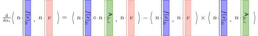
  Figure 6: The visualization of Part 4 of Lemma 5.1. We are given $f(x)_{j_{0}},v,\operatorname{\mathsf{A}}_{j_{0},i}\in\mathbb{R}^{n}$. The left-hand side of the equation is the derivative of the inner product of $f(x)_{j_{0}}$ and $v$ with respect to $x_{i}\in\mathbb{R}$. For the right-hand side, we have three steps. Step 1: we compute the Hadamard product of $f(x)_{j_{0}}$ and $\operatorname{\mathsf{A}}_{j_{0},i}$. Step 2: We find the inner product of this Hadamard product and $v$. Step 3: We subtract the product of two inner products, one is of $f(x)_{j_{0}}$ and $v$ and the other is of $f(x)_{j_{0}}$ and $\operatorname{\mathsf{A}}_{j_{0},i}$, from the result of step 2. The purple rectangles represent the vector $f(x)_{j_{0}}$. The red rectangles represent the vector $v$. The green rectangles represent the vector $\operatorname{\mathsf{A}}_{j_{0},i}$.

• Part 5. For each $i_{0}\in[d]$

  $$\frac{\mathrm{d}c(x,:)_{j_{0},i_{0}}}{\mathrm{d}x_{i}}=\langle f(x)_{j_{0}}\circ\operatorname{\mathsf{A}}_{j_{0},i},v\rangle-\langle f(x)_{j_{0}},v\rangle\cdot\langle f(x)_{j_{0}},\operatorname{\mathsf{A}}_{j_{0},i}\rangle$$

• Part 6.

  $$\frac{\mathrm{d}L(x,:)_{j_{0},i_{0}}}{\mathrm{d}x_{i}}=c(x,:)_{j_{0},i_{0}}\cdot(\langle f(x)_{j_{0}}\circ\operatorname{\mathsf{A}}_{j_{0},i},v\rangle-\langle f(x)_{j_{0}},v\rangle\cdot\langle f(x)_{j_{0}},\operatorname{\mathsf{A}}_{j_{0},i}\rangle)$$

• Part 7. (for hessian diagonal term)

  $$\frac{\mathrm{d}\langle f(x)_{j_{0}}\circ\operatorname{\mathsf{A}}_{j_{0},i},v\rangle}{\mathrm{d}x_{i}}=\langle f(x)_{j_{0}}\circ\operatorname{\mathsf{A}}_{j_{0},i}\circ\operatorname{\mathsf{A}}_{j_{0},i},v\rangle-\langle f(x)_{j_{0}}\circ\operatorname{\mathsf{A}}_{j_{0},i},v\rangle\cdot\langle f(x)_{j_{0}},\operatorname{\mathsf{A}}_{j_{0},i}\rangle$$

  

  Figure 7: The visualization of Part 7 of Lemma 5.1. We are given $f(x)_{j_{0}},v,\operatorname{\mathsf{A}}_{j_{0},i}\in\mathbb{R}^{n}$. First, we compute the Hadamard product between $f(x)_{j_{0}}$ and $\operatorname{\mathsf{A}}_{j_{0},i}$. The left-hand side of the equation is the derivative of the inner product of this Hadamard product and $v$ with respect to $x_{i}\in\mathbb{R}$. For the right-hand side, we have four steps. Step 1: We compute the inner product of the Hadamard product of $f(x)_{j_{0}},\operatorname{\mathsf{A}}_{j_{0},i},\operatorname{\mathsf{A}}_{j_{0},i}$ and $v$. Step 2: We compute the inner product of the Hadamard product of $f(x)_{j_{0}},\operatorname{\mathsf{A}}_{j_{0},i}$ and $v$. Step 3: We compute the inner product between $f(x)_{j_{0}}$ and $\operatorname{\mathsf{A}}_{j_{0},i}$. Step 4: We subtract the product of steps 2 and 3 from step 1. The purple rectangles represent the vector $f(x)_{j_{0}}$. The red rectangles represent the vector $v$. The green rectangles represent the vector $\operatorname{\mathsf{A}}_{j_{0},i}$.

• Part 8. (for hessian off-diagonal term)

  $$\frac{\mathrm{d}\langle f(x)_{j_{0}}\circ\operatorname{\mathsf{A}}_{j_{0},i},v\rangle}{\mathrm{d}x_{l}}=\langle f(x)_{j_{0}}\circ\operatorname{\mathsf{A}}_{j_{0},i}\circ\operatorname{\mathsf{A}}_{j_{0},l},v\rangle-\langle f(x)_{j_{0}}\circ\operatorname{\mathsf{A}}_{j_{0},l},v\rangle\cdot\langle f(x)_{j_{0}},\operatorname{\mathsf{A}}_{j_{0},i}\rangle$$

• Part 9 (for hessian diagonal term, this can be obtained by using Part 4 as a black-box)

  $$\frac{\mathrm{d}\langle f(x)_{j_{0}},\operatorname{\mathsf{A}}_{j_{0},i}\rangle}{\mathrm{d}x_{i}}=\langle f(x)_{j_{0}},\operatorname{\mathsf{A}}_{j_{0},i}\circ\operatorname{\mathsf{A}}_{j_{0},i}\rangle-\langle f(x)_{j_{0}},\operatorname{\mathsf{A}}_{j_{0},i}\rangle\cdot\langle f(x)_{j_{0}},\operatorname{\mathsf{A}}_{j_{0},i}\rangle$$

  

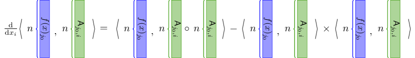
  Figure 8: The visualization of Part 9 of Lemma 5.1. We are given $f(x)_{j_{0}},\operatorname{\mathsf{A}}_{j_{0},i}\in\mathbb{R}^{n}$. The left-hand side of the equation is the derivative of the inner product of $f(x)_{j_{0}}$ and $\operatorname{\mathsf{A}}_{j_{0},i}$ with respect to $x_{i}\in\mathbb{R}$. For the right-hand side, we have three steps. Step 1: we compute the Hadamard product of $\operatorname{\mathsf{A}}_{j_{0},i}$ and $\operatorname{\mathsf{A}}_{j_{0},i}$. Step 2: We find the inner product of $f(x)_{j_{0}}$ and this Hadamard product. Step 3: We subtract the square of inner product of $f(x)_{j_{0}}$ and $\operatorname{\mathsf{A}}_{j_{0},i}$ from the result of step 2. The purple rectangles represent the vector $f(x)_{j_{0}}$. The green rectangles represent the vector $\operatorname{\mathsf{A}}_{j_{0},i}$.

• Part 10 (for hessian off-diagonal term, this can be obtained by using Part 4 as a black-box)

  $$\frac{\mathrm{d}\langle f(x)_{j_{0}},\operatorname{\mathsf{A}}_{j_{0},i}\rangle}{\mathrm{d}x_{l}}=\langle f(x)_{j_{0}},\operatorname{\mathsf{A}}_{j_{0},i}\circ\operatorname{\mathsf{A}}_{j_{0},l}\rangle-\langle f(x)_{j_{0}},\operatorname{\mathsf{A}}_{j_{0},i}\rangle\cdot\langle f(x)_{j_{0}},\operatorname{\mathsf{A}}_{j_{0},l}\rangle$$

Proof.

Proof of Part 1. See Part 4 of Proof of Lemma 5.18 in [72] (Page 14).

Proof of Part 2. See Part 5 of Proof of Lemma 5.18 in [72] (Page 14).

Proof of Part 3. See Part 9 of Proof of Lemma 5.18 in [72] (page 15).

Proof of Part 4. See Part 14 of Proof of Lemma 5.18 in [72] (page 15).

Proof of Part 5.

Note that by Definition 4.12, we have

$$c(x,:)_{j_{0},i_{0}}:=\langle f(x)_{j_{0}},v\rangle-b_{j_{0},i_{0}}$$ (3)

Therefore, we have

$$\frac{\mathrm{d}c(x,:)_{j_{0},i_{0}}}{\mathrm{d}x_{i}}= ~{}\frac{\mathrm{d}(\langle f(x)_{j_{0}},v\rangle-b_{j_{0},i_{0}})}{\mathrm{d}x_{i}}$$

$$= ~{}\frac{\mathrm{d}\langle f(x)_{j_{0}},v\rangle}{\mathrm{d}x_{i}}$$

$$= ~{}\langle f(x)_{j_{0}}\circ\operatorname{\mathsf{A}}_{j_{0},i},v\rangle-\langle f(x)_{j_{0}},v\rangle\cdot\langle f(x)_{j_{0}},\operatorname{\mathsf{A}}_{j_{0},i}\rangle,$$

where the first step comes from Eq. (3), the second step follows from $\frac{\mathrm{d}b_{j_{0},i_{0}}}{\mathrm{d}x_{i}}=0$, and the third step is due to Part 4.

Proof of Part 6. Noted that by Definition 4.13, we have

$$L(x,:)_{j_{0},i_{0}}=0.5c(x,:)_{j_{0},i_{0}}^{2}$$ (4)

Therefore, we have

$$\frac{\mathrm{d}L(x,:)_{j_{0},i_{0}}}{\mathrm{d}x_{i}}= ~{}\frac{\mathrm{d}(0.5c(x,:)_{j_{0},i_{0}}^{2})}{\mathrm{d}x_{i}}$$

$$= ~{}c(x,:)_{j_{0},i_{0}}\frac{\mathrm{d}c(x,:)}{\mathrm{d}x_{i}}$$

$$= ~{}c(x,:)_{j_{0},i_{0}}\cdot(\langle f(x)_{j_{0}}\circ\operatorname{\mathsf{A}}_{j_{0},i},v\rangle-\langle f(x)_{j_{0}},v\rangle\cdot\langle f(x)_{j_{0}},\operatorname{\mathsf{A}}_{j_{0},i}\rangle),$$

where the first step is due to Eq. (4), the second step is because of chain rule of derivative, the last step comes from Part 5.

Proof of Part 7.

We have

$$\frac{\mathrm{d}\langle f(x)_{j_{0}}\circ\operatorname{\mathsf{A}}_{j_{0},i},v\rangle}{\mathrm{d}x_{i}}= ~{}\langle\frac{\mathrm{d}(f(x)_{j_{0}}\circ\operatorname{\mathsf{A}}_{j_{0},i})}{\mathrm{d}x_{i}},v\rangle$$

$$= ~{}\langle\frac{\mathrm{d}f(x)_{j_{0}}}{\mathrm{d}x_{i}}\circ\operatorname{\mathsf{A}}_{j_{0},i},v\rangle$$

$$= ~{}\langle(f(x)_{j_{0}}\circ\operatorname{\mathsf{A}}_{j_{0},i}-f(x)_{j_{0}}\cdot\langle f(x)_{j_{0}},\operatorname{\mathsf{A}}_{j_{0},i}\rangle)\circ\operatorname{\mathsf{A}}_{j_{0},i},v\rangle$$

$$= ~{}\langle f(x)_{j_{0}}\circ\operatorname{\mathsf{A}}_{j_{0},i}\circ\operatorname{\mathsf{A}}_{j_{0},i}-f(x)_{j_{0}}\cdot\langle f(x)_{j_{0}},\operatorname{\mathsf{A}}_{j_{0},i}\rangle\circ\operatorname{\mathsf{A}}_{j_{0},i},v\rangle$$

$$= ~{}\langle f(x)_{j_{0}}\circ\operatorname{\mathsf{A}}_{j_{0},i}\circ\operatorname{\mathsf{A}}_{j_{0},i},v\rangle-\langle f(x)_{j_{0}}\cdot\langle f(x)_{j_{0}},\operatorname{\mathsf{A}}_{j_{0},i}\rangle\circ\operatorname{\mathsf{A}}_{j_{0},i},v\rangle$$

$$= ~{}\langle f(x)_{j_{0}}\circ\operatorname{\mathsf{A}}_{j_{0},i}\circ\operatorname{\mathsf{A}}_{j_{0},i},v\rangle-\langle f(x)_{j_{0}},\operatorname{\mathsf{A}}_{j_{0},i}\rangle\cdot\langle f(x)_{j_{0}}\circ\operatorname{\mathsf{A}}_{j_{0},i},v\rangle$$

where the first step is due to Fact 4.5, the second step comes from Fact 4.5, the third step is because of Part 4, the fourth step is owing to simple algebra, the fifth step follows from Fact 4.1, and the last step comes from Fact 4.1.

Proof of Part 8.

We have

$$\frac{\mathrm{d}\langle f(x)_{j_{0}}\circ\operatorname{\mathsf{A}}_{j_{0},i},v\rangle}{\mathrm{d}x_{l}}= ~{}\langle\frac{\mathrm{d}(f(x)_{j_{0}}\circ\operatorname{\mathsf{A}}_{j_{0},i})}{\mathrm{d}x_{l}},v\rangle$$

$$= ~{}\langle\frac{\mathrm{d}f(x)_{j_{0}}}{\mathrm{d}x_{l}}\circ\operatorname{\mathsf{A}}_{j_{0},i},v\rangle$$

$$= ~{}\langle(f(x)_{j_{0}}\circ\operatorname{\mathsf{A}}_{j_{0},l}-f(x)_{j_{0}}\cdot\langle f(x)_{j_{0}},\operatorname{\mathsf{A}}_{j_{0},l}\rangle)\circ\operatorname{\mathsf{A}}_{j_{0},i},v\rangle$$

$$= ~{}\langle f(x)_{j_{0}}\circ\operatorname{\mathsf{A}}_{j_{0},i}\circ\operatorname{\mathsf{A}}_{j_{0},l}-f(x)_{j_{0}}\cdot\langle f(x)_{j_{0}},\operatorname{\mathsf{A}}_{j_{0},l}\rangle\circ\operatorname{\mathsf{A}}_{j_{0},i},v\rangle$$

$$= ~{}\langle f(x)_{j_{0}}\circ\operatorname{\mathsf{A}}_{j_{0},i}\circ\operatorname{\mathsf{A}}_{j_{0},l},v\rangle-\langle f(x)_{j_{0}}\cdot\langle f(x)_{j_{0}},\operatorname{\mathsf{A}}_{j_{0},l}\rangle\circ\operatorname{\mathsf{A}}_{j_{0},i},v\rangle$$

$$= ~{}\langle f(x)_{j_{0}}\circ\operatorname{\mathsf{A}}_{j_{0},i}\circ\operatorname{\mathsf{A}}_{j_{0},l},v\rangle-\langle f(x)_{j_{0}},\operatorname{\mathsf{A}}_{j_{0},l}\rangle\cdot\langle f(x)_{j_{0}}\circ\operatorname{\mathsf{A}}_{j_{0},i},v\rangle$$

where the first step comes from Fact 4.5, the second step is because of Fact 4.5, the third step follows from Part 4, the fourth step is due to simple algebra, the fifth step is owing to Fact 4.1, and the last step comes from Fact 4.1.

Proof of Part 9.

We have

$$\frac{\mathrm{d}\langle f(x)_{j_{0}},\operatorname{\mathsf{A}}_{j_{0},i}\rangle}{\mathrm{d}x_{i}}= ~{}\langle\frac{\mathrm{d}f(x)_{j_{0}}}{\mathrm{d}x_{i}},\operatorname{\mathsf{A}}_{j_{0},i}\rangle$$

$$= ~{}\langle f(x)_{j_{0}}\circ\operatorname{\mathsf{A}}_{j_{0},i}-f(x)_{j_{0}}\cdot\langle f(x)_{j_{0}},\operatorname{\mathsf{A}}_{j_{0},i}\rangle,\operatorname{\mathsf{A}}_{j_{0},i}\rangle$$

$$= ~{}\langle f(x)_{j_{0}},\operatorname{\mathsf{A}}_{j_{0},i}\circ\operatorname{\mathsf{A}}_{j_{0},i}\rangle-\langle f(x)_{j_{0}},\operatorname{\mathsf{A}}_{j_{0},i}\rangle\cdot\langle f(x)_{j_{0}},\operatorname{\mathsf{A}}_{j_{0},i}\rangle$$

where the first step is due to Fact 4.5, the second step comes from Part 4, and the last step is because of Fact 4.1.

Proof of Part 10. We have

$$\frac{\mathrm{d}\langle f(x)_{j_{0}},\operatorname{\mathsf{A}}_{j_{0},i}\rangle}{\mathrm{d}x_{l}}= ~{}\langle\frac{\mathrm{d}f(x)_{j_{0}}}{\mathrm{d}x_{l}},\operatorname{\mathsf{A}}_{j_{0},i}\rangle$$

$$= ~{}\langle f(x)_{j_{0}}\circ\operatorname{\mathsf{A}}_{j_{0},l}-f(x)_{j_{0}}\cdot\langle f(x)_{j_{0}},\operatorname{\mathsf{A}}_{j_{0},l}\rangle,\operatorname{\mathsf{A}}_{j_{0},i}\rangle$$

$$= ~{}\langle f(x)_{j_{0}},\operatorname{\mathsf{A}}_{j_{0},i}\circ\operatorname{\mathsf{A}}_{j_{0},l}\rangle-\langle f(x)_{j_{0}},\operatorname{\mathsf{A}}_{j_{0},i}\rangle\cdot\langle f(x)_{j_{0}},\operatorname{\mathsf{A}}_{j_{0},l}\rangle$$

where the first step comes from Fact 4.5, the second step is owing to Part 4, and the last step is due to Fact 4.1. ∎

5.2 Gradient With Respect to $y$

In this section, we compute the gradient with respect to $y$.

Lemma 5.2.

If the following conditions hold

• Let $v\in\mathbb{R}^{n}$ which doesn’t depend on x and also doesn’t depend on y.

• Let $c(:,y)_{j_{0},i_{0}}\in\mathbb{R}$ be defined as Definition 4.12.

• Let $L(:,y)_{j_{0},i_{0}}\in\mathbb{R}$ be defined as Definition 4.13.

• Let $h(y_{i_{0}}):=\underbrace{A_{3}}_{n\times d}\underbrace{y_{i_{0}}}_{d\times 1}.$

• Let $h(y_{i_{0}})=h(y)_{i_{0}}$ for convenient

• Let $A_{3,*,i_{2}}\in\mathbb{R}^{n}$ denote the $i_{2}$-th column of matrix $A_{3}\in\mathbb{R}^{n\times d}$ for each $i_{2}\in[d]$

Then, we have

• Part 1. If $i_{1}=i_{0}$

  $$\frac{\mathrm{d}h(y_{i_{0}})}{\mathrm{d}y_{i_{1},i_{2}}}=A_{3,*,i_{2}}$$

• Part 2. If $i_{1}\neq i_{0}$

  $$\frac{\mathrm{d}h(y_{i_{0}})}{\mathrm{d}y_{i_{1},i_{2}}}={\bf 0}_{n}$$

• Part 3. If $i_{1}=i_{0}$

  $$\frac{\mathrm{d}\langle v,h(y)_{i_{0}}\rangle}{\mathrm{d}y_{i_{1},i_{2}}}=\langle v,A_{3,*,i_{2}}\rangle$$

• Part 4. If $i_{1}\neq i_{0}$

  $$\frac{\mathrm{d}\langle v,h(y)_{i_{0}}\rangle}{\mathrm{d}y_{i_{1},i_{2}}}=0$$

• Part 5. If $i_{1}=i_{0}$

  $$\frac{\mathrm{d}c(:,y)_{j_{0},i_{0}}}{\mathrm{d}y_{i_{1},i_{2}}}=\langle v,A_{3,*,i_{2}}\rangle$$

• Part 6. If $i_{1}\neq i_{0}$

  $$\frac{\mathrm{d}c(:,y)_{j_{0},i_{0}}}{\mathrm{d}y_{i_{1},i_{2}}}=0$$

• Part 7. If $i_{1}=i_{0}$

  $$\frac{\mathrm{d}L(:,y)_{j_{0},i_{0}}}{\mathrm{d}y_{i_{1},i_{2}}}=c(:,y)_{j_{0},i_{0}}\langle v,A_{3,*,i_{2}}\rangle$$

• Part 8. If $i_{1}\neq i_{0}$

  $$\frac{\mathrm{d}L(:,y)_{j_{0},i_{0}}}{\mathrm{d}y_{i_{1},i_{2}}}=0$$

Proof.

Proof of Part 1.

$$\frac{\mathrm{d}h(y_{i_{0}})}{\mathrm{d}y_{i_{1},i_{2}}}= ~{}\frac{\mathrm{d}A_{3}y_{i_{0}}}{\mathrm{d}y_{i_{1},i_{2}}}$$

$$= ~{}A_{3,*,i_{2}}$$

where the first step is due to the definition of $h(y_{i_{0}})$ (see the Lemma statement), and the last step comes from that for $i\neq i_{2},~{}\frac{\mathrm{d}}{\mathrm{d}y_{i_{2}}}f(y_{i})=0$.

Proof of Part 2.

$$\frac{\mathrm{d}h(y_{i_{0}})}{\mathrm{d}y_{i_{1},i_{2}}}= ~{}{\bf 0}_{n}$$

where the first step is due to $i_{1}\neq i_{2}$.

Proof of Part 3.

$$\frac{\mathrm{d}\langle v,h(y)_{i_{0}}\rangle}{\mathrm{d}y_{i_{1},i_{2}}}= ~{}\langle v,\frac{\mathrm{d}h(y_{i_{0}})}{\mathrm{d}y_{i_{1},i_{2}}}\rangle$$

$$= ~{}\langle v,A_{3,*,i_{2}}\rangle$$

where the first step comes from Fact 4.5, the second step is due to the result of Part 1.

Proof of Part 4.

$$\frac{\mathrm{d}\langle v,h(y)_{i_{0}}\rangle}{\mathrm{d}y_{i_{1},i_{2}}}= ~{}\langle v,\frac{\mathrm{d}h(y_{i_{0}})}{\mathrm{d}y_{i_{1},i_{2}}}\rangle$$

$$= ~{}0$$

where the first step is becaues of Fact 4.5, the second step comes from the result of Part 2.

Proof of Part 5.

$$\frac{\mathrm{d}c(:,y)_{j_{0},i_{0}}}{\mathrm{d}y_{i_{1},i_{2}}}= ~{}\frac{\mathrm{d}\langle v,h(y)_{i_{0}}\rangle-b_{j_{0},i_{0}}}{\mathrm{d}y_{i_{1},i_{2}}}$$

$$\ = ~{}\frac{\mathrm{d}\langle v,h(y)_{i_{0}}\rangle}{\mathrm{d}y_{i_{1},i_{2}}}$$

$$= ~{}\langle v,A_{3,*,i_{2}}\rangle$$

where the first step comes from the Definition 4.12, the second step is because of $\frac{\mathrm{d}b_{j_{0},i_{0}}}{\mathrm{d}y_{i_{1},i_{2}}}=0$, and the last step is due to Part 3.

Proof of Part 6.

$$\frac{\mathrm{d}c(:,y)_{j_{0},i_{0}}}{\mathrm{d}y_{i_{1},i_{2}}}= ~{}\frac{\mathrm{d}\langle v,h(y)_{i_{0}}\rangle-b_{j_{0},i_{0}}}{\mathrm{d}y_{i_{1},i_{2}}}$$

$$\ = ~{}\frac{\mathrm{d}\langle v,h(y)_{i_{0}}\rangle}{\mathrm{d}y_{i_{1},i_{2}}}$$

$$= ~{}0$$

where the first step is due to the Definition 4.12, the second step comes from $\frac{\mathrm{d}b_{j_{0},i_{0}}}{\mathrm{d}y_{i_{1},i_{2}}}=0$, and the last step is owing to Part 4.

Proof of Part 7.

$$\frac{\mathrm{d}L(:,y)_{j_{0},i_{0}}}{\mathrm{d}y_{i_{1},i_{2}}}= ~{}\frac{\mathrm{d}0.5c(:,y)_{j_{0},i_{0}}^{2}}{\mathrm{d}y_{i_{1},i_{2}}}$$

$$= ~{}c(:,y)_{j_{0},i_{0}}\cdot\frac{\mathrm{d}c(:,y)_{j_{0},i_{0}}}{\mathrm{d}y_{i_{1},i_{2}}}$$

$$= ~{}c(:,y)_{j_{0},i_{0}}\langle v,A_{3,*,i_{2}}\rangle$$

where the first step is due to the Definition 4.13, the second step comes from the chain rule of derivative, and the last step is owing to Part 5.

Proof of Part 8.

$$\frac{\mathrm{d}L(:,y)_{j_{0},i_{0}}}{\mathrm{d}y_{i_{1},i_{2}}}= ~{}\frac{\mathrm{d}0.5c(:,y)_{j_{0},i_{0}}^{2}}{\mathrm{d}y_{i_{1},i_{2}}}$$

$$= ~{}c(:,y)_{j_{0},i_{0}}\cdot\frac{\mathrm{d}c(:,y)_{j_{0},i_{0}}}{\mathrm{d}y_{i_{1},i_{2}}}$$

$$= ~{}0$$

where the first step is because of the Definition 4.13, the second step is due to the chain rule of derivative, and the last step comes from Part 6. ∎

5.3 Computation of $c,f,h$

In this section, we explain how to compute $c(x,y),f(x),h(y)$.

Lemma 5.3.

If the following conditions hold

• For each $j_{0}\in[n]$, $i_{0}\in[d]$, let $c(x,y)_{j_{0},i_{0}}\in\mathbb{R}$ be defined as Definition 4.12. (We can view $c(x,y)$ as an $n\times d$ matrix)

• For each $j_{0}\in[n]$, let $f(x)_{j_{0}}\in\mathbb{R}^{n}$ be defined as Definition 4.10. (We can view $f(x)$ as an $n\times n$ matrix)

• For each $i_{0}\in[d]$, let $h(y)_{i_{0}}\in\mathbb{R}^{n}$ be defined as Definition 4.11. (We can view $h(y)$ as $n\times d$ matrix)

• Let $A_{3}\in\mathbb{R}^{n\times d}$

• We can view $y$ as an $d\times d$ matrix

Then, we can compute $f,h,c$ in $O({\cal T}_{\mathrm{mat}}(n,d,d)+{\cal T}_{\mathrm{mat}}(n,n,d))$ time.

Proof.

By definition 4.11, we have

$$\underbrace{h(y)}_{n\times d}=\underbrace{A_{3}}_{n\times d}\underbrace{y}_{d\times d}.$$ (5)

First $h(y)\in\mathbb{R}^{n\times d}$ can be viewed as multiplying $n\times d$ matrix ($A_{3}$) and $d\times d$ matrix ($y$), this can be computed in ${\cal T}_{\mathrm{mat}}(n,d,d)$.

Figure 9: The visualization of Eq. (5). We have $A_{3}\in\mathbb{R}^{n\times d}$. $h:\mathbb{R}^{d\times d}\to\mathbb{R}^{n\times d}$ is a function, which maps the matrix $y\in\mathbb{R}^{d\times d}$ to $h(y)$ by multiplying $A_{3}$ and $y$. The red rectangles represent matrices which are the factors, and the blue rectangle represents the matrix which is the product.

We also have

$$\underbrace{f(x)}_{n\times n}=\underbrace{D(X)^{-1}}_{n\times n}\exp(\underbrace{A_{1}}_{n\times d}\underbrace{X}_{d\times d}\underbrace{A_{2}^{\top}}_{d\times n}),\mathrm{~{}~{}~{}and~{}~{}~{}}D(X)=\operatorname{diag}(\exp(A_{1}XA_{2}^{\top}){\bf 1}_{n})$$ (6)

Then the computation of $f(x)\in\mathbb{R}^{n\times n}$ can be done in ${\cal T}_{\mathrm{mat}}(n,n,d)+{\cal T}_{\mathrm{mat}}(n,d,d)$.

Figure 10: The visualization of Eq. (6). We have $A_{1},A_{2}\in\mathbb{R}^{n\times d}$, $X\in\mathbb{R}^{d\times d}$, and $D(X)\in\mathbb{R}^{n\times n}$ (see Definition 1.2 and Figure 1). First, we find the inverse of the matrix $D(X)$ and compute $\exp(A_{1}XA_{2}^{\top})\in\mathbb{R}^{n\times n}$, as shown in Figure 1. Then, we multiply $D(X)^{-1}$ and $\exp(A_{1}XA_{2}^{\top})$ to get $f(x)\in\mathbb{R}^{n\times n}$. The green squares represent the square matrices in $\mathbb{R}^{n\times n}$. The blue rectangles represent the matrices in $\mathbb{R}^{n\times d}$ (the dark blue denotes the transpose of the matrix in $\mathbb{R}^{n\times d}$). The red square represents the square matrices in $\mathbb{R}^{d\times d}$.

Given that

$$\underbrace{c(x,y)}_{n\times d}=\underbrace{f(x)}_{n\times n}\underbrace{h(y)}_{n\times d}-\underbrace{B}_{n\times d}$$ (7)

Then $c$ can be done in ${\cal T}_{\mathrm{mat}}(n,n,d)$.

Figure 11: The visualization of Eq. (7). Let $f(x)\in\mathbb{R}^{n\times n}$ (see Figure 10) and $h(y)\in\mathbb{R}^{n\times d}$ (see Figure 9). We have $B\in\mathbb{R}^{n\times d}$. We multiply $f(x)$ with $h(y)$ and subtract $B$ from their product to get $c(x,y)\in\mathbb{R}^{n\times d}$. The green square represents the square matrices in $\mathbb{R}^{n\times n}$. The blue rectangles represent the matrix in $\mathbb{R}^{n\times d}$.

∎

5.4 Reformulating Gradient ($x$) in Matrix View

In this section, we reformulate the gradient $x$ in the matrix’s view.

Lemma 5.4.

If the following conditions hold

• $\frac{\mathrm{d}L(x,y)_{j_{0},i_{0}}}{\mathrm{d}x_{i}}=c(x,y)_{j_{0},i_{0}}\cdot(\langle f(x)_{j_{0}}\circ\operatorname{\mathsf{A}}_{j_{0},i},h(y)_{i_{0}}\rangle-\langle f(x)_{j_{0}},h(y)_{i_{0}}\rangle\cdot\langle f(x)_{j_{0}},\operatorname{\mathsf{A}}_{j_{0},i}\rangle)$

• Let $c(x,y)\in\mathbb{R}^{n\times d}$

• Let $f(x)_{j_{0}}\in\mathbb{R}^{n}$

• Let $h(y)_{i_{0}}\in\mathbb{R}^{n}$

• Let $\frac{\mathrm{d}L(x,y)}{\mathrm{d}x}=\sum_{j_{0}=1}^{n}\sum_{i_{0}=1}^{d}\frac{\mathrm{d}L(x,y)_{j_{0},i_{0}}}{\mathrm{d}x}$

• Let

  $$q(x,y)_{j_{0}}=\sum_{i_{0}=1}^{d}c(x,y)_{j_{0},i_{0}}h(y)_{i_{0}}$$

then, we have

• Part 1.

  $$\frac{\mathrm{d}L(x,y)_{j_{0},i_{0}}}{\mathrm{d}x}=\underbrace{c(x,:)_{j_{0},i_{0}}}_{\mathrm{scalar}}\cdot\underbrace{\operatorname{\mathsf{A}}_{j_{0}}^{\top}}_{d^{2}\times n}\underbrace{(f(x)_{j_{0}}-f(x)_{j_{0}}f(x)_{j_{0}}^{\top})}_{n\times n}\underbrace{h(y)_{i_{0}}}_{n\times 1}$$

• Part 2. Suppose $c(x,y),\operatorname{\mathsf{A}},f(x),h(y)$ are given, then $\frac{\mathrm{d}L(x,y)_{j_{0},i_{0}}}{\mathrm{d}x}$ can be computed in $O(nd^{2})$ time.

• Part 3.

  $$\frac{\mathrm{d}L(x,y)}{\mathrm{d}x}=\sum_{j_{0}=1}^{n}\operatorname{\mathsf{A}}_{j_{0}}^{\top}(f(x)_{j_{0}}-f(x)_{j_{0}}f(x)_{j_{0}})q(x,y)_{j_{0}}$$

• Part 4. Suppose $c(x,y),\operatorname{\mathsf{A}},f(x),h(y)$ are given, then $\frac{\mathrm{d}L(x,y)}{\mathrm{d}x}\in\mathbb{R}^{d^{2}}$ can be computed in ${\cal T}_{\mathrm{mat}}(n,d,n)+{\cal T}_{\mathrm{mat}}(n,d,d)$ time

Proof.

Proof of Part 1.

Note that by Fact 4.1, we have

$$\langle f(x)_{j_{0}}\circ\operatorname{\mathsf{A}}_{j_{0},i},h(y)_{i_{0}}\rangle=\operatorname{\mathsf{A}}_{j_{0},i}^{\top}\operatorname{diag}(f(x)_{j_{0}})h(y)_{i_{0}}$$

and

$$\langle f(x)_{j_{0}},v\rangle\cdot\langle f(x)_{j_{0}},\operatorname{\mathsf{A}}_{j_{0},i}\rangle=\operatorname{\mathsf{A}}_{j_{0},i}^{\top}f(x)_{j_{0}}f(x)_{j_{0}}^{\top}h(y)_{i_{0}}$$

Thus, we complete the proof.

Proof of Part 2.

We first compute $(\operatorname{diag}(f(x)_{j_{0}})-f(x)_{j_{0}}f(x)_{j_{0}}^{\top})h(y)_{i_{0}}$, this can be done in $O(n)$ time.

Then we can compute the rest, it takes $O(nd^{2})$ time.

Proof of Part 3 and Part 4.

Firstly, we can compute $q(x,y)_{j_{0}}\in\mathbb{R}^{n}$.

Recall from the Lemma statement, we have

$$q(x,y)_{j_{0}}=\sum_{i_{0}=1}^{d}c(x,y)_{j_{0},i_{0}}h(y)_{i_{0}}.$$ (8)

Let $q(x,y)_{j_{0}}\in\mathbb{R}^{n}$ denote the $j_{0}$-th column of $q(x,y)$.

Then we have

$$q(x,y)=\underbrace{h(y)}_{n\times d}\underbrace{c(x,y)^{\top}}_{d\times n}$$

This takes ${\cal T}_{\mathrm{mat}}(n,d,n)$ time.

Then, we compute

$$p(x,y)_{j_{0}}=(\operatorname{diag}(f(x)_{j_{0}})-f(x)_{j_{0}}f(x)_{j_{0}})q(x,y)_{j_{0}}.$$ (9)

This takes $O(n^{2})$ time in total.

We can show that

$$~{}\frac{\mathrm{d}L(x,y)}{\mathrm{d}x}$$

$$= ~{}\sum_{j_{0}=1}^{n}\sum_{i_{0}=1}^{d}\frac{\mathrm{d}L(x,y)_{j_{0},i_{0}}}{\mathrm{d}x}$$

$$= ~{}\sum_{j_{0}=1}^{n}\sum_{i_{0}=1}^{d}\underbrace{c(x,y)_{j_{0},i_{0}}}_{\mathrm{scalar}}\cdot\underbrace{\operatorname{\mathsf{A}}_{j_{0}}^{\top}}_{d^{2}\times n}\underbrace{(\operatorname{diag}(f(x)_{j_{0}})-f(x)_{j_{0}}f(x)_{j_{0}}^{\top})}_{n\times n}\underbrace{h(y)_{i_{0}}}_{n\times 1}$$

$$= ~{}\sum_{j_{0}=1}^{n}\operatorname{\mathsf{A}}_{j_{0}}^{\top}(\operatorname{diag}(f(x)_{j_{0}})-f(x)_{j_{0}}f(x)_{j_{0}})q(x,y)_{j_{0}}$$

$$= ~{}\sum_{j_{0}=1}^{n}\operatorname{\mathsf{A}}_{j_{0}}^{\top}p(x,y)_{j_{0}}$$

$$= ~{}\operatorname{vec}(A_{1}^{\top}p(x,y)A_{2})$$

where the first step is based on Definition 4.7, the second step is because of Part 1, the third step is due to Eq. (8), the fourth step follows from Eq. (9), and the last step due to tensor-trick.

Note that $A_{1}^{\top}p(x,y)A_{2}$ can be computed in ${\cal T}_{\mathrm{mat}}(n,d,n)+{\cal T}_{\mathrm{mat}}(d,n,d)$ time. ∎

5.5 Reformulating Gradient ($y$) in Matrix View

In this section, we reformulate the gradient $y$ in the matrix’s view.

Lemma 5.5.

If the following conditions hold

• if $i_{1}=i_{0}$, $\frac{\mathrm{d}L(x,y)_{j_{0},i_{0}}}{\mathrm{d}y_{i_{1},i_{2}}}=c(x,y)_{j_{0},i_{0}}\langle f(x)_{j_{0}},A_{3,*,i_{2}}\rangle$

• if $i_{1}\neq i_{0}$, $\frac{\mathrm{d}L(x,y)_{j_{0},i_{0}}}{\mathrm{d}y_{i_{1},i_{2}}}=0$

• Let $\frac{\mathrm{d}L(x,y)}{\mathrm{d}y_{i_{0},i_{2}}}=\sum_{j_{0}=1}^{n}c(x,y)_{j_{0},i_{0}}\langle f(x)_{j_{0}},A_{3,*,i_{2}}\rangle$

• Let $\widetilde{q}(x,y)_{i_{0}}=\sum_{j_{0}=1}^{n}f(x)_{j_{0}}c(x,y)_{j_{0},i_{0}}$

Then we have

• Part 1.

  $$\frac{\mathrm{d}L(x,y)_{j_{0},i_{0}}}{\mathrm{d}y_{i_{0},i_{2}}}=A_{3,*,i_{2}}^{\top}f(x)_{j_{0}}c(x,y)_{j_{0},i_{0}}$$

• Part 2.

  $$\frac{\mathrm{d}L(x,y)}{\mathrm{d}y_{i_{0},i_{2}}}=A_{3,*,i_{2}}^{\top}\widetilde{q}(x,y)_{i_{0}}$$

• Part 3.

  $$\frac{\mathrm{d}L(x,y)}{\mathrm{d}y}=\operatorname{vec}(\underbrace{A_{3}^{\top}}_{d\times n}\underbrace{\widetilde{q}(x,y)}_{n\times d})$$

• Part 4. Computing $\frac{\mathrm{d}L(x,y)}{\mathrm{d}y}$ takes ${\cal T}_{\mathrm{mat}}(n,n,d)+{\cal T}_{\mathrm{mat}}(n,d,d)$

Proof.

Proof of Part 1.

$$\frac{\mathrm{d}L(x,y)_{j_{0},i_{0}}}{\mathrm{d}y_{i_{0},i_{2}}}= ~{}c(x,y)_{j_{0},i_{0}}\langle f(x)_{j_{0}},A_{3,*,i_{2}}\rangle$$

$$= ~{}A_{3,*,i_{2}}^{\top}f(x)_{j_{0}}c(x,y)_{j_{0},i_{0}}$$

where the first step comes from the assumption from the Lemma statement and the second step is based on Fact 4.1.

Proof of Part 2.

$$\frac{\mathrm{d}L(x,y)}{\mathrm{d}y_{i_{0},i_{2}}}= ~{}\sum_{j_{0}=1}^{n}c(x,y)_{j_{0},i_{0}}\langle f(x)_{j_{0}},A_{3,*,i_{2}}\rangle$$

$$= ~{}\sum_{j_{0}=1}^{n}A_{3,*,i_{2}}^{\top}f(x)_{j_{0}}c(x,y)_{j_{0},i_{0}}$$

$$= ~{}A_{3,*,i_{2}}^{\top}\widetilde{q}(x,y)_{i_{0}}$$

where the first step is due to the assumption from the Lemma statement, the second step is because of Fact 4.1, and the last step comes from the definition of $\widetilde{q}(x,y)_{i_{0}}$ (see from the Lemma statement).

Proof of Part 3.

$$\frac{\mathrm{d}L(x,y)}{\mathrm{d}y}=\operatorname{vec}(A_{3}^{\top}\widetilde{q}(x,y))$$

where the first step comes from tensor trick based on Part 2.

Proof of Part 4. Computing $\widetilde{q}(x,y)\in\mathbb{R}^{n\times d}$ takes ${\cal T}_{\mathrm{mat}}(n,n,d)$ time.

Computing $A_{3}^{\top}\widetilde{q}(x,y)$ takes ${\cal T}_{\mathrm{mat}}(n,d,d)$ time.

∎

6 Hessian

In this section, we provide more details related to Hessian.

Finally the hessian $H\in\mathbb{R}^{2d^{2}\times 2d^{2}}$ which can be written as

$$H=\begin{bmatrix}H_{x,x}&H_{x,y}\\ H_{y,x}&H_{y,y}\end{bmatrix}$$

where

• $H_{x,x}\in\mathbb{R}^{d^{2}\times d^{2}}$ is $\frac{\mathrm{d}^{2}L}{\mathrm{d}x\mathrm{d}x}$ (see details in Section 7)

• $H_{x,y}$, $H_{y,x}\in\mathbb{R}^{d^{2}\times d^{2}}$ is $\frac{\mathrm{d}^{2}L}{\mathrm{d}x\mathrm{d}y}$ (see details in Section 11)

• $H_{y,y}\in\mathbb{R}^{d^{2}\times d^{2}}$ is $\frac{\mathrm{d}^{2}L}{\mathrm{d}y\mathrm{d}y}$ (see details in Section 10)

  • We can view $H_{y,y}=\begin{bmatrix}H_{y,y,1,1}&0&0&\cdots&0\\ 0&H_{y,y,2,2}&0&\cdots&0\\ 0&0&H_{y,y,3,3}&\cdots&0\\ \vdots&\vdots&\vdots&\ddots&\vdots\\ 0&0&0&\cdots&H_{y,y,d,d}\end{bmatrix}$

  • where $H_{y,y,i_{0},i_{0}}=\sum_{j_{0}=1}^{n}\frac{\mathrm{d}^{2}L_{j_{0},i_{0}}}{\mathrm{d}y_{i_{0},*}\mathrm{d}y_{i_{0},*}}\in\mathbb{R}^{d\times d}$ for each $i_{0}\in[d]$

Lemma 6.1.

If the following conditions hold

• $H_{x,x}\succeq\alpha_{1}I_{d^{2}}$

• $H_{y,y}\succeq\alpha_{2}I_{d^{2}}$

• $\|H_{x,y}\|\leq\alpha_{3}$

• $\|H_{y,x}\|\leq\alpha_{3}$

• Let $\alpha_{1}\geq\alpha_{3}>0$, $\alpha_{2}\geq\alpha_{3}>0$

Then we have

$$H\succeq\{\alpha_{1}-\alpha_{3},\alpha_{2}-\alpha_{3}\}\cdot I_{2d^{2}}$$

Proof.

Let $u,v\in\mathbb{R}^{d^{2}}$, then we have

$$\begin{bmatrix}u^{\top}&v^{\top}\end{bmatrix}H\begin{bmatrix}u\\ v\end{bmatrix}= ~{}u^{\top}H_{x,x}u+v^{\top}H_{y,y}v+u^{\top}H_{x,y}v+v^{\top}H_{y,x}u$$

$$\geq ~{}\|u\|_{2}^{2}\cdot\alpha_{1}+\|v\|_{2}^{2}\cdot\alpha_{2}+u^{\top}H_{x,y}v+v^{\top}H_{y,x}u$$

$$\geq ~{}\|u\|_{2}^{2}\cdot\alpha_{1}+\|v\|_{2}^{2}\cdot\alpha_{2}-\|u\|_{2}\|v\|_{2}(\|H_{x,y}\|+\|H_{y,x}\|)$$

$$\geq ~{}\|u\|_{2}^{2}\cdot\alpha_{1}+\|v\|_{2}^{2}\cdot\alpha_{2}-\|u\|_{2}\|v\|_{2}2\alpha_{3}$$

$$\geq ~{}\|u\|_{2}^{2}\cdot\alpha_{1}+\|v\|_{2}^{2}\cdot\alpha_{2}-(\|u\|_{2}^{2}+\|v\|_{2}^{2})\alpha_{3}$$

$$\geq ~{}(\|u\|_{2}^{2}+\|v\|_{2}^{2})\cdot\min\{\alpha_{1}-\alpha_{3},\alpha_{2}-\alpha_{3}\}$$

where the first step is based on the expansion of $H$, the second step is due to $H_{x,x}\succeq\alpha_{1}I_{d^{2}},H_{y,y}\succeq\alpha_{2}I_{d^{2}}$, the third step comes from Fact 4.2 and Fact 4.3 , the fourth step is because of $\|H_{x,y}\|\leq\alpha_{3},\|H_{y,x}\|\leq\alpha_{3}$, the fifth step is owing to $2\|u\|_{2}\|v\|_{2}\leq\|u\|_{2}^{2}+\|v\|_{2}^{2}$, and the last step is based on the simple algebra.

Thus, it implies

$$H\succeq\{\alpha_{1}-\alpha_{3},\alpha_{2}-\alpha_{3}\}\cdot I_{2d^{2}}$$

∎

Algorithm 1 Our Algorithm

1:procedure TrainingAlgorithm($A_{1},A_{2},A_{3},B\in\mathbb{R}^{n\times d}$) $\triangleright$ Theorem 1.3

2:     Let $x(0),y(0)\in\mathbb{R}^{d^{2}}$ denote initialization point

3:     for $t=0\to T-1$ do

4:          /*Forward*/

5:         Compute $h(y(t))\in\mathbb{R}^{n\times d}$ $\triangleright$ ${\cal T}_{\mathrm{mat}}(n,d,d)$ time

6:         Compute $f(x(t))\in\mathbb{R}^{n\times n}$ $\triangleright$ ${\cal T}_{\mathrm{mat}}(n,d,n)$ time

7:         Compute $c(x(t),y(t))\in\mathbb{R}^{n\times d}$ (based on $f(x(t))$, $h(y(t))$) $\triangleright$ ${\cal T}_{\mathrm{mat}}(n,d,d)$ time

8:          /*Gradient*/

9:         Compute $g(x(t))$ based on Lemma 5.4 $\triangleright$ ${\cal T}_{\mathrm{mat}}(n,d,n)+{\cal T}_{\mathrm{mat}}(n,d,d)$ time

10:         Compute $g(y(t))$ based on Lemma 5.5 $\triangleright$ ${\cal T}_{\mathrm{mat}}(n,d,n)+{\cal T}_{\mathrm{mat}}(n,d,d)$ time

11:          /*Hessian*/

12:         Compute $\widetilde{H}$ via TensorSRHT $\triangleright$ $\widetilde{O}(nd+d^{2\omega})$

13:          /*Update*/

14:         $\begin{bmatrix}x(t+1)\\ y(t+1)\end{bmatrix}\leftarrow\begin{bmatrix}x(t)\\ y(t)\end{bmatrix}-\begin{bmatrix}g(x(t))\\ g(y(t))\end{bmatrix}\widetilde{H}^{-1}$ $\triangleright$ $O(d^{2\omega})$

15:     end for

16:end procedure

7 Hessian for $X$

In Section 7.1, we compute the Hessian matrix with respect to $x$. In Section 7.2, we present a helpful lemma to simplify the Hessian. In Section 7.3, we define $B(x)$, representing the Hessian.

7.1 Hessian

Now, we start to compute the Hessian matrix with respect to $x$.

Lemma 7.1.

If the following conditions hold

• Let $\gamma(x)_{j_{0}}:=\langle f(x)_{j_{0}},v\rangle$ (We define this notation for easy of writing proofs.)

Then we have for each $i\in[d^{2}]$, $l\in[d^{2}]$

• Part 1. $i=l$ Hessian diagonal term

  $$\frac{\mathrm{d}^{2}L_{j_{0},i_{0}}}{\mathrm{d}x_{i}\mathrm{d}x_{i}}= ~{}(\langle f(x)_{j_{0}}\circ\operatorname{\mathsf{A}}_{j_{0},i},v\rangle-\gamma_{j_{0}}(x)\cdot\langle f(x)_{j_{0}},\operatorname{\mathsf{A}}_{j_{0},i}\rangle)^{2}$$

  $$~{}+c(x,:)_{j_{0},i_{0}}\cdot$$

  $$~{}($$

  $$~{}+\langle f(x)_{j_{0}}\circ\operatorname{\mathsf{A}}_{j_{0},i}\circ\operatorname{\mathsf{A}}_{j_{0},i},v\rangle(1-\gamma_{j_{0}}(x))$$

  $$~{}-2\langle f(x)_{j_{0}}\circ\operatorname{\mathsf{A}}_{j_{0},i},v\rangle\cdot\langle f(x)_{j_{0}},\operatorname{\mathsf{A}}_{j_{0},i}\rangle$$

  $$~{}+2\langle f(x)_{j_{0}},\operatorname{\mathsf{A}}_{j_{0},i}\rangle^{2}\cdot\gamma_{j_{0}}(x)$$

  $$~{})$$

• Part 2. $i\neq l$ Hessian off-diagonal term

  $$\frac{\mathrm{d}^{2}L_{j_{0},i_{0}}}{\mathrm{d}x_{i}\mathrm{d}x_{l}}= ~{}(\langle f(x)_{j_{0}}\circ\operatorname{\mathsf{A}}_{j_{0},i},v\rangle-\gamma_{j_{0}}(x)\cdot\langle f(x)_{j_{0}},\operatorname{\mathsf{A}}_{j_{0},i}\rangle)$$

  $$~{}\cdot(\langle f(x)_{j_{0}}\circ\operatorname{\mathsf{A}}_{j_{0},l},v\rangle-\gamma_{j_{0}}(x)\cdot\langle f(x)_{j_{0}},\operatorname{\mathsf{A}}_{j_{0},l}\rangle)$$

  $$~{}+c(x,:)_{j_{0},i_{0}}\cdot$$

  $$~{}($$

  $$~{}+\langle f(x)_{j_{0}}\circ\operatorname{\mathsf{A}}_{j_{0},i}\circ\operatorname{\mathsf{A}}_{j_{0},l},v\rangle(1-\langle f(x)_{j_{0}},v\rangle))$$

  $$~{}-\langle f(x)_{j_{0}}\circ\operatorname{\mathsf{A}}_{j_{0},i},v\rangle\cdot\langle f(x)_{j_{0}},\operatorname{\mathsf{A}}_{j_{0},l}\rangle-\langle f(x)_{j_{0}}\circ\operatorname{\mathsf{A}}_{j_{0},l},v\rangle\cdot\langle f(x)_{j_{0}},\operatorname{\mathsf{A}}_{j_{0},i}\rangle$$

  $$~{}+2\langle f(x)_{j_{0}},\operatorname{\mathsf{A}}_{j_{0},i}\rangle\langle f(x)_{j_{0}},\operatorname{\mathsf{A}}_{j_{0},l}\rangle\cdot\gamma_{j_{0}}(x)$$

  $$~{})$$

Proof.

Proof of Part 1.

At first, we have

$$~{}\frac{\mathrm{d}}{\mathrm{d}x_{i}}(\langle f(x)_{j_{0}}\circ\operatorname{\mathsf{A}}_{j_{0},i},v\rangle-\langle f(x)_{j_{0}},v\rangle\cdot\langle f(x)_{j_{0}},\operatorname{\mathsf{A}}_{j_{0},i}\rangle)$$

$$= ~{}\underbrace{\frac{\mathrm{d}}{\mathrm{d}x_{i}}\langle f(x)_{j_{0}}\circ\operatorname{\mathsf{A}}_{j_{0},i},v\rangle}_{\mathrm{Part~{}7~{}of~{}Lemma~{}\ref{lem:gradient_x}}}$$

$$~{}-\underbrace{(\frac{\mathrm{d}}{\mathrm{d}x_{i}}\langle f(x)_{j_{0}},v\rangle)}_{{\mathrm{Part~{}4~{}of~{}Lemma~{}\ref{lem:gradient_x}}}}\cdot\langle f(x)_{j_{0}},\operatorname{\mathsf{A}}_{j_{0},i}\rangle$$

$$~{}-\underbrace{(\frac{\mathrm{d}}{\mathrm{d}x_{i}}\langle f(x)_{j_{0}},\operatorname{\mathsf{A}}_{j_{0},i}\rangle)}_{{\mathrm{Part~{}9~{}of~{}Lemma~{}\ref{lem:gradient_x}}}}\cdot\langle f(x)_{j_{0}},v\rangle$$

$$= ~{}\langle f(x)_{j_{0}}\circ\operatorname{\mathsf{A}}_{j_{0},i}\circ\operatorname{\mathsf{A}}_{j_{0},i},v\rangle-\langle f(x)_{j_{0}}\circ\operatorname{\mathsf{A}}_{j_{0},i},v\rangle\cdot\langle f(x)_{j_{0}},\operatorname{\mathsf{A}}_{j_{0},i}\rangle$$

$$~{}-(\langle f(x)_{j_{0}}\circ\operatorname{\mathsf{A}}_{j_{0},i},v\rangle-\langle f(x)_{j_{0}},v\rangle\cdot\langle f(x)_{j_{0}},\operatorname{\mathsf{A}}_{j_{0},i}\rangle)\cdot\langle f(x)_{j_{0}},\operatorname{\mathsf{A}}_{j_{0},i}\rangle$$

$$~{}-(\langle f(x)_{j_{0}}\circ\operatorname{\mathsf{A}}_{j_{0},i},\operatorname{\mathsf{A}}_{j_{0},i}\rangle-\langle f(x)_{j_{0}},\operatorname{\mathsf{A}}_{j_{0},i}\rangle\langle f(x)_{j_{0}},\operatorname{\mathsf{A}}_{j_{0},i}\rangle)\cdot\langle f(x)_{j_{0}},v\rangle$$

$$= ~{}\langle f(x)_{j_{0}}\circ\operatorname{\mathsf{A}}_{j_{0},i}\circ\operatorname{\mathsf{A}}_{j_{0},i},v\rangle$$

$$~{}-2\langle f(x)_{j_{0}}\circ\operatorname{\mathsf{A}}_{j_{0},i},v\rangle\cdot\langle f(x)_{j_{0}},\operatorname{\mathsf{A}}_{j_{0},i}\rangle$$

$$~{}+2\langle f(x)_{j_{0}},\operatorname{\mathsf{A}}_{j_{0},i}\rangle^{2}\cdot\langle f(x)_{j_{0}},v\rangle$$

$$~{}-\langle f(x)_{j_{0}}\circ\operatorname{\mathsf{A}}_{j_{0},i}\circ\operatorname{\mathsf{A}}_{j_{0},i},v\rangle\cdot\langle f(x)_{j_{0}},v\rangle$$

where the first step is based on the product rule of derivative, the second step comes from Part 4, Part 7, and Part 9 of Lemma 5.1, and the last step is due to simple algebra.

Then we can show that

$$~{}\frac{\mathrm{d}}{\mathrm{d}x_{i}}(\frac{\mathrm{d}}{\mathrm{d}x_{i}}L_{j_{0},i_{0}})$$

$$= ~{}\frac{\mathrm{d}}{\mathrm{d}x_{i}}(c(x,:)_{j_{0},i_{0}}\cdot(\langle f(x)_{j_{0}}\circ\operatorname{\mathsf{A}}_{j_{0},i},v\rangle-\langle f(x)_{j_{0}},v\rangle\cdot\langle f(x)_{j_{0}},\operatorname{\mathsf{A}}_{j_{0},i}\rangle))$$

$$= ~{}(\langle f(x)_{j_{0}}\circ\operatorname{\mathsf{A}}_{j_{0},i},v\rangle-\langle f(x)_{j_{0}},v\rangle\cdot\langle f(x)_{j_{0}},\operatorname{\mathsf{A}}_{j_{0},i}\rangle)^{2}$$

$$~{}+c(x,:)_{j_{0},i_{0}}\cdot\frac{\mathrm{d}}{\mathrm{d}x_{i}}(\langle f(x)_{j_{0}}\circ\operatorname{\mathsf{A}}_{j_{0},i},v\rangle-\langle f(x)_{j_{0}},v\rangle\cdot\langle f(x)_{j_{0}},\operatorname{\mathsf{A}}_{j_{0},i}\rangle),$$

where the first step comes from Part 6 of Lemma 5.1 and the second step is due to Part 5 of Lemma 5.1.

Combining the above two equations, we complete the proof.

Proof of Part 2.

Firstly, we can show that

$$~{}\frac{\mathrm{d}}{\mathrm{d}x_{l}}(\langle f(x)_{j_{0}}\circ\operatorname{\mathsf{A}}_{j_{0},i},v\rangle-\langle f(x)_{j_{0}},v\rangle\cdot\langle f(x)_{j_{0}},\operatorname{\mathsf{A}}_{j_{0},i}\rangle)$$

$$= ~{}\underbrace{\frac{\mathrm{d}}{\mathrm{d}x_{l}}\langle f(x)_{j_{0}}\circ\operatorname{\mathsf{A}}_{j_{0},i},v\rangle}_{\mathrm{Part~{}8~{}of~{}Lemma~{}\ref{lem:gradient_x}}}$$

$$~{}-\underbrace{(\frac{\mathrm{d}}{\mathrm{d}x_{l}}\langle f(x)_{j_{0}},v\rangle)}_{{\mathrm{Part~{}4~{}of~{}Lemma~{}\ref{lem:gradient_x}}}}\cdot\langle f(x)_{j_{0}},\operatorname{\mathsf{A}}_{j_{0},i}\rangle$$

$$~{}-\underbrace{(\frac{\mathrm{d}}{\mathrm{d}x_{l}}\langle f(x)_{j_{0}},\operatorname{\mathsf{A}}_{j_{0},i}\rangle)}_{{\mathrm{Part~{}10~{}of~{}Lemma~{}\ref{lem:gradient_x}}}}\cdot\langle f(x)_{j_{0}},v\rangle$$

$$= ~{}\langle f(x)_{j_{0}}\circ\operatorname{\mathsf{A}}_{j_{0},i}\circ\operatorname{\mathsf{A}}_{j_{0},l},v\rangle-\langle f(x)_{j_{0}}\circ\operatorname{\mathsf{A}}_{j_{0},l},v\rangle\cdot\langle f(x)_{j_{0}},\operatorname{\mathsf{A}}_{j_{0},i}\rangle$$

$$~{}-(\langle f(x)_{j_{0}}\circ\operatorname{\mathsf{A}}_{j_{0},l},v\rangle-\langle f(x)_{j_{0}},v\rangle\cdot\langle f(x)_{j_{0}},\operatorname{\mathsf{A}}_{j_{0},l}\rangle)\cdot\langle f(x)_{j_{0}},\operatorname{\mathsf{A}}_{j_{0},i}\rangle$$

$$~{}-(\langle f(x)_{j_{0}}\circ\operatorname{\mathsf{A}}_{j_{0},i},\operatorname{\mathsf{A}}_{j_{0},l}\rangle-\langle f(x)_{j_{0}},\operatorname{\mathsf{A}}_{j_{0},i}\rangle\langle f(x)_{j_{0}},\operatorname{\mathsf{A}}_{j_{0},l}\rangle)\cdot\langle f(x)_{j_{0}},v\rangle$$

$$= ~{}\langle f(x)_{j_{0}}\circ\operatorname{\mathsf{A}}_{j_{0},i}\circ\operatorname{\mathsf{A}}_{j_{0},l},v\rangle$$

$$~{}-\langle f(x)_{j_{0}}\circ\operatorname{\mathsf{A}}_{j_{0},i},v\rangle\cdot\langle f(x)_{j_{0}},\operatorname{\mathsf{A}}_{j_{0},l}\rangle-\langle f(x)_{j_{0}}\circ\operatorname{\mathsf{A}}_{j_{0},l},v\rangle\cdot\langle f(x)_{j_{0}},\operatorname{\mathsf{A}}_{j_{0},i}\rangle$$

$$~{}+2\langle f(x)_{j_{0}},\operatorname{\mathsf{A}}_{j_{0},i}\rangle\langle f(x)_{j_{0}},\operatorname{\mathsf{A}}_{j_{0},l}\rangle\cdot\langle f(x)_{j_{0}},v\rangle$$

$$~{}-\langle f(x)_{j_{0}}\circ\operatorname{\mathsf{A}}_{j_{0},i}\circ\operatorname{\mathsf{A}}_{j_{0},l},v\rangle\cdot\langle f(x)_{j_{0}},v\rangle$$

where the first step is owing to the product rule of derivative, the second step is based on Part 4, Part 8, and Part 10 of Lemma 5.1, and the last step comes from simple algebra.

We have

$$~{}\frac{\mathrm{d}}{\mathrm{d}x_{l}}(\frac{\mathrm{d}}{\mathrm{d}x_{i}}L_{j_{0},i_{0}})$$

$$= ~{}\frac{\mathrm{d}}{\mathrm{d}x_{l}}(c(x,:)_{j_{0},i_{0}}\cdot(\langle f(x)_{j_{0}}\circ\operatorname{\mathsf{A}}_{j_{0},i},v\rangle-\langle f(x)_{j_{0}},v\rangle\cdot\langle f(x)_{j_{0}},\operatorname{\mathsf{A}}_{j_{0},i}\rangle))$$

$$= ~{}(\langle f(x)_{j_{0}}\circ\operatorname{\mathsf{A}}_{j_{0},i},v\rangle-\langle f(x)_{j_{0}},v\rangle\cdot\langle f(x)_{j_{0}},\operatorname{\mathsf{A}}_{j_{0},i}\rangle)$$

$$~{}\cdot(\langle f(x)_{j_{0}}\circ\operatorname{\mathsf{A}}_{j_{0},l},v\rangle-\langle f(x)_{j_{0}},v\rangle\cdot\langle f(x)_{j_{0}},\operatorname{\mathsf{A}}_{j_{0},l}\rangle)$$

$$~{}+c(x,:)_{j_{0},i_{0}}\cdot\frac{\mathrm{d}}{\mathrm{d}x_{l}}(\langle f(x)_{j_{0}}\circ\operatorname{\mathsf{A}}_{j_{0},i},v\rangle-\langle f(x)_{j_{0}},v\rangle\cdot\langle f(x)_{j_{0}},\operatorname{\mathsf{A}}_{j_{0},i}\rangle)$$

Combining the above two equations, we complete the proof. ∎

7.2 A Helpful Lemma

In this section, we present a helpful Lemma.

Lemma 7.2.

We have

• Part 1.

  $$\langle f(x)_{j_{0}}\circ\operatorname{\mathsf{A}}_{j_{0},i}\circ\operatorname{\mathsf{A}}_{j_{0},l},v\rangle=\underbrace{\operatorname{\mathsf{A}}_{j_{0},i}^{\top}}_{d^{2}\times n}\underbrace{\operatorname{diag}(f(x)_{j_{0}}\circ v)}_{n\times n}\underbrace{\operatorname{\mathsf{A}}_{j_{0},l}}_{n\times d^{2}}$$

• Part 2.

  $$~{}\langle f(x)_{j_{0}}\circ\operatorname{\mathsf{A}}_{j_{0},i},v\rangle\cdot\langle f(x)_{j_{0}},\operatorname{\mathsf{A}}_{j_{0},l}\rangle+\langle f(x)_{j_{0}}\circ\operatorname{\mathsf{A}}_{j_{0},l},v\rangle\cdot\langle f(x)_{j_{0}},\operatorname{\mathsf{A}}_{j_{0},i}\rangle$$

  $$= ~{}\operatorname{\mathsf{A}}_{j_{0},i}^{\top}(\underbrace{(f(x)_{j_{0}}\circ v)(f(x)_{j_{0}})^{\top}+f(x)_{j_{0}}(f(x)_{j_{0}}\circ v)^{\top}}_{\operatorname{rank}-2})\operatorname{\mathsf{A}}_{j_{0},l}$$

• Part 3.

  $$\langle f(x)_{j_{0}}\circ\operatorname{\mathsf{A}}_{j_{0},i},v\rangle\cdot\langle f(x)_{j_{0}}\circ\operatorname{\mathsf{A}}_{j_{0},l},v\rangle=\operatorname{\mathsf{A}}_{j_{0},i}^{\top}\underbrace{(f(x)_{j_{0}}\circ v)(f(x)_{j_{0}}\circ v)^{\top}}_{\operatorname{rank}-1}\operatorname{\mathsf{A}}_{j_{0},l}$$

• Part 4.

  $$\langle f(x)_{j_{0}},\operatorname{\mathsf{A}}_{j_{0},i}\rangle\cdot\langle f(x)_{j_{0}},\operatorname{\mathsf{A}}_{j_{0},l}\rangle=\operatorname{\mathsf{A}}_{j_{0},i}^{\top}\underbrace{(f(x)_{j_{0}})(f(x)_{j_{0}})^{\top}}_{\operatorname{rank}-1}\operatorname{\mathsf{A}}_{j_{0},l}$$

Proof.

Proof of Part 1. We have

$$\langle f(x)_{j_{0}}\circ\operatorname{\mathsf{A}}_{j_{0},i}\circ\operatorname{\mathsf{A}}_{j_{0},l},v\rangle= ~{}\operatorname{\mathsf{A}}_{j_{0},i}^{\top}\operatorname{diag}(f(x)_{j_{0}}\circ v)\operatorname{\mathsf{A}}_{j_{0},l}$$

where the first step follows from Fact 4.1.

Proof of Part 2. We have

$$~{}\langle f(x)_{j_{0}}\circ\operatorname{\mathsf{A}}_{j_{0},i},v\rangle\cdot\langle f(x)_{j_{0}},\operatorname{\mathsf{A}}_{j_{0},l}\rangle+\langle f(x)_{j_{0}}\circ\operatorname{\mathsf{A}}_{j_{0},l},v\rangle\cdot\langle f(x)_{j_{0}},\operatorname{\mathsf{A}}_{j_{0},i}\rangle$$

$$= ~{}\langle f(x)_{j_{0}}\circ v,\operatorname{\mathsf{A}}_{j_{0},i}\rangle\cdot f(x)_{j_{0}}^{\top}\operatorname{\mathsf{A}}_{j_{0},l}$$

$$~{}+\langle f(x)_{j_{0}}\circ v,\operatorname{\mathsf{A}}_{j_{0},l}\rangle\cdot\operatorname{\mathsf{A}}_{j_{0},i}^{\top}\cdot f(x)_{j_{0}}$$

$$= ~{}\operatorname{\mathsf{A}}_{j_{0},i}^{\top}\cdot(f(x)_{j_{0}}\circ v)(f(x)_{j_{0}})^{\top}\operatorname{\mathsf{A}}_{j_{0},i}$$

$$~{}+\operatorname{\mathsf{A}}_{j_{0},i}^{\top}f(x)_{j_{0}}(f(x)_{j_{0}}\circ v)^{\top}\operatorname{\mathsf{A}}_{j_{0},l}$$

$$= ~{}\operatorname{\mathsf{A}}_{j_{0},i}^{\top}((f(x)_{j_{0}}\circ v)(f(x)_{j_{0}})^{\top}$$

$$~{}+f(x)_{j_{0}}(f(x)_{j_{0}}\circ v)^{\top})\operatorname{\mathsf{A}}_{j_{0},l}$$

where the first step follows from Fact 4.1, the second step follows from Fact 4.1, and the last step follows from the simple algebra.

Proof of Part 3. We have

$$\langle f(x)_{j_{0}}\circ\operatorname{\mathsf{A}}_{j_{0},i},v\rangle\cdot\langle f(x)_{j_{0}}\circ\operatorname{\mathsf{A}}_{j_{0},l},v\rangle= ~{}\langle f(x)_{j_{0}}\circ v,\operatorname{\mathsf{A}}_{j_{0},i}\rangle\langle f(x)_{j_{0}}\circ v,\operatorname{\mathsf{A}}_{j_{0},l}\rangle$$

$$= ~{}\operatorname{\mathsf{A}}_{j_{0},i}^{\top}(f(x)_{j_{0}}\circ v)(f(x)_{j_{0}}\circ v)^{\top}\operatorname{\mathsf{A}}_{j_{0},l}$$

where the first step follows from Fact 4.1, and the last step follows from Fact 4.1.

Proof of Part 4. We have

$$\langle f(x)_{j_{0}},\operatorname{\mathsf{A}}_{j_{0},i}\rangle\cdot\langle f(x)_{j_{0}},\operatorname{\mathsf{A}}_{j_{0},l}\rangle= ~{}\operatorname{\mathsf{A}}_{j_{0},i}^{\top}f(x)_{j_{0}}f(x)_{j_{0}}^{\top}\operatorname{\mathsf{A}}_{j_{0},l}$$

where the first step follows from Fact 4.1. ∎

7.3 Defining $B(x)$

In this section, we formally define $B(x)$.

Definition 7.3.

If the following conditions hold

• Let $\gamma_{j_{0}}(x)=\langle f(x)_{j_{0}},v\rangle$

We define $B(x)\in\mathbb{R}^{n\times n}$ as follows

$$B(x):= B_{\operatorname{diag}}^{1}$$

$$~{}+B_{\operatorname{rank}}^{1}+B_{\operatorname{rank}}^{2}+B_{\operatorname{rank}}^{3}$$

where

• $B_{\operatorname{diag}}^{1}:=(1-\gamma_{j_{0}}(x))\cdot c(x,:)_{j_{0},i_{0}}\cdot\operatorname{diag}(f(x)_{j_{0}}\circ v)$

and

• $B_{\operatorname{rank}}^{1}:=-(2\gamma_{j_{0}}(x)+c(x,:)_{j_{0},i_{0}})\cdot((f(x)_{j_{0}}\circ v)f(x)_{j_{0}}^{\top}+f(x)_{j_{0}}(f(x)_{j_{0}}\circ v)^{\top})$

• $B_{\operatorname{rank}}^{2}:=(2\gamma_{j_{0}}(x)c(x,:)_{j_{0},i_{0}}+\gamma_{j_{0}}(x)^{2})\cdot f(x)_{j_{0}}f(x)_{j_{0}}^{\top}$

• $B_{\operatorname{rank}}^{3}:=(f(x)_{j_{0}}\circ v)\cdot(f(x)_{j_{0}}\circ v)^{\top}$

Lemma 7.4.

Let $B(x)$ be defined as Definition 7.3, then we have

$$\frac{\mathrm{d}^{2}L_{j_{0},i_{0}}}{\mathrm{d}x\mathrm{d}x}=\underbrace{\operatorname{\mathsf{A}}_{j_{0}}^{\top}}_{d^{2}\times n}\underbrace{B(x)}_{n\times n}\underbrace{\operatorname{\mathsf{A}}_{j_{0}}}_{n\times d^{2}}$$

Proof.

The proof follows by combining Lemma 7.1 and Lemma 7.2. ∎

8 Lipschitz Property of $H_{x,x}$

In Section 8.1, we present the main results of the Lipschitz property of $H_{x,x}$. In Section 8.2, we summarize the results from following steps 1-9. In Section 8.3, we compute the upper bound of basic functions for the following proof. In Section 8.4, we compute the Lipschitz Property of basic functions for the following proof. In Section 8.5, we analyze the first step of Lipschitz function $c(x,:)_{j_{0},i_{0}}\cdot\operatorname{diag}(f(x)_{j_{0}}\circ v)$. In Section 8.6, we analyze the second step of Lipschitz function $-\gamma_{j_{0}}(x)\cdot c(x,:)_{j_{0},i_{0}}\cdot\operatorname{diag}(f(x)_{j_{0}}\circ v)$. In Section 8.7, we analyze the third step of Lipschitz function $-2\gamma_{j_{0}}(x)\cdot(f(x)_{j_{0}}\circ v)f(x)_{j_{0}}^{\top}$. In Section 8.8, we analyze the fourth step of Lipschitz function $-c(x,:)_{j_{0},i_{0}}\cdot(f(x)_{j_{0}}\circ v)f(x)_{j_{0}}^{\top}$. In Section 8.9, we analyze the fifth step of Lipschitz function $-2\gamma_{j_{0}}(x)\cdot f(x)_{j_{0}}(f(x)_{j_{0}}\circ v)^{\top}$. In Section 8.10, we analyze the sixth step of Lipschitz function $-c(x,:)_{j_{0},i_{0}})\cdot f(x)_{j_{0}}(f(x)_{j_{0}}\circ v)^{\top}$. In Section 8.11, we analyze the seventh step of Lipschitz function $2\gamma_{j_{0}}(x)c(x,:)_{j_{0},i_{0}}\cdot f(x)_{j_{0}}f(x)_{j_{0}}^{\top}$. In Section 8.12, we analyze the eighth step of Lipschitz function $\gamma_{j_{0}}(x)^{2}\cdot f(x)_{j_{0}}f(x)_{j_{0}}^{\top}$. In Section 8.13, we analyze the nineth step of Lipschitz function $(f(x)_{j_{0}}\circ v)\cdot(f(x)_{j_{0}}\circ v)^{\top}$.

8.1 Main Result

In this section, we present the main result of the Lipschitz property.

Lemma 8.1.

If the following conditions hold

• Let $H_{j_{0},i_{0}}=\frac{\mathrm{d}^{2}L_{j_{0},i_{0}}}{\mathrm{d}x\mathrm{d}x}:\mathbb{R}^{d^{2}}\rightarrow\mathbb{R}^{d^{2}\times d^{2}}$

• Let $H=\sum_{j_{0}=1}^{n}\sum_{i_{0}=1}^{d}H_{j_{0},i_{0}}$ (because $L=\sum_{j_{0}=1}^{n}\sum_{i_{0}=1}^{d}L_{j_{0},i_{0}}$)

• Let $\operatorname{\mathsf{A}}\in\mathbb{R}^{n^{2}\times d^{2}}$ and $u(x)_{j_{0}}\in\mathbb{R}^{n}$ be defined as Definition 4.8

• Let $\alpha(x)_{j_{0}}\in\mathbb{R}$ be defined as Definition 4.9

• Let $f(x)_{j_{0}}\in\mathbb{R}^{n}$ be defined as Definition 4.10

• Let $c(x,:)_{j_{0},i_{0}}\in\mathbb{R}$ be defined as Definition 4.12

• Let $\gamma(x)_{j_{0}}=\langle f(x)_{j_{0}},v\rangle\in\mathbb{R}$

• $\|A_{1}\|,\|A_{2}\|,\|A_{3}\|\leq R$, $\|\operatorname{\mathsf{A}}_{j_{0}}\|\leq R$, $\|x\|_{2}\leq R$,$|b_{j_{0},i_{0}}|\leq R$, $\|v\|_{2}\leq R^{2}$

• Let $R\geq 4$

• Let $M:=\exp(O(R^{2}+\log(nd)))$

Then, we have for all $x,\widetilde{x}\in\mathbb{R}^{d^{2}}$

• Part 1. For each $j_{0}\in[n]$, $i_{0}\in[d]$

  $$\|H_{j_{0},i_{0}}(x)-H_{j_{0},i_{0}}(\widetilde{x})\|\leq M\cdot\|x-\widetilde{x}\|_{2}$$

• Part 2.

  $$\|H(x)-H(\widetilde{x})\|\leq M\cdot\|x-\widetilde{x}\|_{2}$$

Proof.

Proof of Part 1. We have

$$\|H_{j_{0},i_{0}}(x)-H_{j_{0},i_{0}}(\widetilde{x})\|\leq ~{}\sum_{k=1}^{9}\|\operatorname{\mathsf{A}}_{j_{0}}^{\top}\|\cdot\|G_{k}(x)-G_{k}(\widetilde{x})\|\cdot\|\operatorname{\mathsf{A}}_{j_{0}}\|$$

$$\leq ~{}9R^{2}\cdot n^{1.5}\exp(20R^{2})$$

$$\leq ~{}n^{1.5}\exp(30R^{2})$$

where the first step follows from definition of $H_{j_{0},i_{0}}(x)$, the second step follows from Lemma 8.2, and last step follows from simple algebra.

Proof of Part 2.

Then, we have

$$\|H(x)-H(\widetilde{x})\|\leq ~{}\sum_{j_{0}=1}^{n}\sum_{i_{0}=1}^{d}\|H_{j_{0},i_{0}}(x)-H_{j_{0},i_{0}}(\widetilde{x})\|$$

$$\leq ~{}nd\cdot n^{1.5}\exp(30R^{2})$$

where the first step follows from triangle inequality and $H=\sum_{j_{0}=1}^{n}\sum_{i_{0}=1}^{d}H_{j_{0},i_{0}}$, and the second step follows from Part 1. ∎

8.2 Summary of Nine Steps

In this section, we provide a summary of the nine-step calculation of Lipschitz for different matrix functions.

Lemma 8.2.

If the following conditions hold

• $G_{1}(x)=c(x,:)_{j_{0},i_{0}}\cdot\operatorname{diag}(f(x)_{j_{0}}\circ v)$

• $G_{2}(x)=-\gamma_{j_{0}}(x)\cdot c(x,:)_{j_{0},i_{0}}\cdot\operatorname{diag}(f(x)_{j_{0}}\circ v)$

• $G_{3}(x)=-2\gamma_{j_{0}}(x)\cdot(f(x)_{j_{0}}\circ v)f(x)_{j_{0}}^{\top}$

• $G_{4}(x)=-c(x,:)_{j_{0},i_{0}}\cdot(f(x)_{j_{0}}\circ v)f(x)_{j_{0}}^{\top}$

• $G_{5}(x)=-2\gamma_{j_{0}}(x)\cdot f(x)_{j_{0}}(f(x)_{j_{0}}\circ v)^{\top}$ (The proof of this is identical to $G_{3}$)

• $G_{6}(x)=-c(x,:)_{j_{0},i_{0}}\cdot f(x)_{j_{0}}(f(x)_{j_{0}}\circ v)^{\top}$ (The proof of this is identical to $G_{4}$)

• $G_{7}(x)=2\gamma_{j_{0}}(x)c(x,:)_{j_{0},i_{0}}\cdot f(x)_{j_{0}}f(x)_{j_{0}}^{\top}$

• $G_{8}(x)=\gamma_{j_{0}}(x)^{2}\cdot f(x)_{j_{0}}f(x)_{j_{0}}^{\top}$

• $G_{9}(x)=(f(x)_{j_{0}}\circ v)\cdot(f(x)_{j_{0}}\circ v)^{\top}$

Then, we have

$$\max_{k\in[9]}\|G_{k}(x)-G_{k}(\widetilde{x})\|\leq n^{1.5}\exp(20R^{2}).$$

Proof.

The proof follows from Lemma 8.7, Lemma 8.8, Lemma 8.9, Lemma 8.10, Lemma 8.11, Lemma 8.12, Lemma 8.13, Lemma 8.14, and Lemma 8.15. ∎

8.3 A Core Tool: Upper Bound for Several Basic Functions

In this section, we analyze the upper bound of several basic functions.

Lemma 8.3 ([55, 72]).

Provided that the subsequent requirements are satisfied

• Let $\operatorname{\mathsf{A}}\in\mathbb{R}^{n^{2}\times d^{2}}$ satisfy $\max_{j_{0}\in[n]}\|\operatorname{\mathsf{A}}_{j_{0}}\|\leq R$

• Let $x\in\mathbb{R}^{d^{2}}$ satisfy that $\|x\|_{2}\leq R$

• We define $u(x)$ as Definition 4.8

• Let $\beta$ be the greatest lower bound of $\langle u(x)_{j_{0}},{\bf 1}_{n}\rangle$

Then we have

$$\beta\geq\exp(-R^{2}).$$

Lemma 8.4 (Basic Functions Upper Bound).

If the following conditions hold,

• Let $u(x)_{j_{0}}\in\mathbb{R}^{n}$ be defined as Definition 4.8

• Let $\alpha(x)_{j_{0}}\in\mathbb{R}$ be defined as Definition 4.9

• Let $f(x)_{j_{0}}\in\mathbb{R}^{n}$ be defined as Definition 4.10

• Let $c(x,:)_{j_{0},i_{0}}\in\mathbb{R}$ be defined as Definition 4.12

• Let $\gamma(x)_{j_{0}}=\langle f(x)_{j_{0}},v\rangle\in\mathbb{R}$

• Let $\beta$ be the greatest lower bound of $\langle u(x)_{j_{0}},{\bf 1}_{n}\rangle$

• $\|A_{1}\|,\|A_{2}\|,\|A_{3}\|\leq R$

• $\|\operatorname{\mathsf{A}}_{j_{0}}\|\leq R$

• $\|x\|_{2}\leq R$

• $|b_{j_{0},i_{0}}|\leq R$

• Let $R\geq 4$

• $\|v\|_{2}\leq R^{2}$

Then we have: for all $x\in\mathbb{R}^{d^{2}}$

• Part 1. $\|u(x)_{j_{0}}\|_{2}\leq\sqrt{n}\cdot\exp(R^{2})$

• Part 2. $|\alpha(x)_{j_{0}}|\leq n\exp(R^{2})$

• Part 3. $|\alpha(x)_{j_{0}}|^{-1}\leq\exp(R^{2})$

• Part 4. $\|f(x)_{j_{0}}\|_{2}\leq 1$

• Part 5. $|\gamma(x)_{j_{0}}|\leq R^{2}$

• Part 6. $|c(x,:)_{j_{0},i_{0}}|\leq 2R^{2}$

Proof.

We present our proof as follows.

Proof of Part 1. We have

$$\|u(x)_{j_{0}}\|_{2}= ~{}\|\exp{\operatorname{\mathsf{A}}_{j_{0}}x}\|_{2}$$

$$\leq ~{}\sqrt{n}\cdot\|\exp(\operatorname{\mathsf{A}}_{j_{0}}x)\|_{\infty}$$

$$\leq ~{}\sqrt{n}\cdot\exp(\|\operatorname{\mathsf{A}}_{j_{0}}x\|_{2})$$

$$\leq ~{}\sqrt{n}\cdot\exp(R^{2})$$

where the first step follows from Definition 4.8, the second step is based on Fact 4.2, the third step follows from Fact 4.2, and the fourth step is because of $\|\operatorname{\mathsf{A}}_{j_{0}}\|\leq R$ and $\|x\|_{2}\leq R$ (see from the Lemma statement).

Proof of Part 2. We have

$$|\alpha(x)_{j_{0}}|= ~{}|\langle u(x)_{j_{0}},{\bf 1}_{n}\rangle|$$

$$\leq ~{}\sqrt{n}\cdot\|u(x)_{j_{0}}\|_{2}$$

$$\leq ~{}\sqrt{n}\cdot\sqrt{n}\cdot\exp(R^{2})$$

$$= ~{}n\exp(R^{2})$$

where the first step is due to Definition 4.9, the second is based on Fact 4.2, the third step follows from Part 1. and the forth step follows from simple algebra.

Proof of Part 3.

We have

$$|\alpha^{-1}(x)_{j_{0}}|= ~{}\frac{1}{\langle u(x)_{j_{0}},{\bf 1}_{n}\rangle}$$

$$\leq ~{}\frac{1}{\beta}$$

$$\leq ~{}\exp(R^{2})$$

where the first step is because of Definition 4.9, the second step follows from the definition of $\beta$ and the third step is due to Lemma 8.3.

Proof of Part 4. We have

$$\|f(x)_{j_{0}}\|_{2}\leq ~{}\|f(x)_{j_{0}}\|_{1}$$

$$= ~{}1$$

where the first step follows from Fact 4.2, the second step is due to Definition 4.10

Proof of Part 5. We have

$$|\gamma(x)_{j_{0}}|= ~{}|\langle f(x)_{j_{0}},v\rangle|$$

$$\leq ~{}\|f(x)_{j_{0}}\|_{2}\cdot\|v\|_{2}$$

$$\leq ~{}1\cdot R^{2}$$

$$= ~{}R^{2}$$

where the first step follows from the definition of $\gamma(x)_{j_{0}}$ (see from the Lemma statement), the second step follows from Cauchy–Schwarz inequality, the third step follows from Part 2 and the upper bound for the $\ell_{2}$ norm of $v$ (from the Lemma statement), and the last step follows from simple algebra.

Proof of Part 6. We have

$$|c(x,:)_{j_{0},i_{0}}|= ~{}|\langle f(x)_{j_{0}},v\rangle-b_{j_{0},i_{0}}|$$

$$\leq ~{}|\gamma_{j_{0}}(x)-b_{j_{0},i_{0}}|$$

$$\leq ~{}|\gamma_{j_{0}}(x)|+|b_{j_{0},i_{0}}|$$

$$\leq ~{}R^{2}+R$$

$$\leq ~{}2R^{2}$$

where the first step is based on Definition 4.12, the second step is because of the definition of $\gamma_{j_{0}}(x)$, the third step follows from triangle inequality, the fourth step is based on Part 6 and $|b_{j_{0},i_{0}}|\leq R$ (see from the Lemma statement), and the last step follows from $R\geq 1$. ∎

8.4 A Core Tool: Lipschitz Property for Several Basic Functions

In this section, we analyze the Lipschitz property of several basic functions.

Lemma 8.5 (Basic Functions Lipschitz Property).

If the following conditions hold,

• $\|v\|\leq R^{2}$

• $\|\operatorname{\mathsf{A}}_{j_{0}}\|\leq R$

• Let $\beta$ be the greatest lower bound of $\langle u(x)_{j_{0}},{\bf 1}_{n}\rangle$

• Let $\beta^{-1}\leq\exp(R^{2})$

• Let $R\geq 4$

Then, we have: for all $x,\widetilde{x}\in\mathbb{R}^{d^{2}}$

• Part 1. $\|u(x)_{j_{0}}-u(\widetilde{x})_{j_{0}}\|_{2}\leq\sqrt{n}\exp(2R^{2})\cdot\|x-\widetilde{x}\|_{2}$

• Part 2. $|\alpha(x)^{-1}-\alpha^{-1}(\widetilde{x})|\leq n\exp(4R^{2})\cdot\|x-\widetilde{x}\|_{2}$

• Part 3. $\|f(x)_{j_{0}}-f(\widetilde{x})_{j_{0}}\|_{2}\leq n^{1.5}R\exp(6R^{2})\cdot\|x-\widetilde{x}\|_{2}$

• Part 4. $|\gamma(x)_{j_{0}}-\gamma(\widetilde{x})_{j_{0}}|\leq n^{1.5}\exp(7R^{2})\cdot\|x-\widetilde{x}\|_{2}$

• Part 5. $|c(x,:)_{j_{0},i_{0}}-c(\widetilde{x},:)_{j_{0},i_{0}}|\leq n^{1.5}\exp(7R^{2})\cdot\|x-\widetilde{x}\|_{2}$

Proof.

Proof of Part 1.

$$\|u(x)_{j_{0}}-u(\widetilde{x})_{j_{0}}\|_{2}= ~{}\|\exp(\operatorname{\mathsf{A}}_{j_{0}}x)-\exp(\operatorname{\mathsf{A}}_{j_{0}}\widetilde{x})\|_{2}$$

$$\leq ~{}\exp(\|\operatorname{\mathsf{A}}_{j_{0}}x\|_{2})\cdot 2\|\operatorname{\mathsf{A}}_{j_{0}}(x-\widetilde{x})\|_{\infty}$$

$$\leq ~{}\sqrt{n}\exp(R^{2})\cdot 2\|\operatorname{\mathsf{A}}_{j_{0}}(x-\widetilde{x})\|_{2}$$

$$\leq ~{}\sqrt{n}\exp(R^{2})\cdot 2\|\operatorname{\mathsf{A}}_{j_{0}}\|\cdot\|x-\widetilde{x}\|_{2}$$

$$\leq ~{}2\sqrt{n}R\exp(R^{2})\cdot\|x-\widetilde{x}\|_{2}$$

$$\leq ~{}\sqrt{n}\exp(2R^{2})\cdot\|x-\widetilde{x}\|_{2}$$

where the first step is due to Definition 4.8, the second step is because of Fact 4.2, the third step is based on Fact 4.2, the fourth step follows from Fact 4.3 , fifth step is due to $\|\operatorname{\mathsf{A}}_{j_{0}}\|\leq R$.

Proof of Part 2 We have

$$|\alpha(x)^{-1}_{j_{0}}-\alpha(\widetilde{x})^{-1}_{j_{0}}|\leq ~{}\alpha(x)^{-1}\alpha(\widetilde{x})^{-1}\cdot|\alpha(x)-\alpha(\widetilde{x})|$$

$$\leq ~{}\beta^{-2}\cdot|\alpha(x)-\alpha(\widetilde{x})|$$

$$\leq ~{}\beta^{-2}\cdot|\langle u(x)_{j_{0}},{\bf 1}_{n}\rangle-\langle u(\widetilde{x})_{j_{0}},{\bf 1}_{n}\rangle|$$

$$\leq ~{}\beta^{-2}\cdot\sqrt{n}\|u(x)_{j_{0}}-u(\widetilde{x})_{j_{0}}\|_{2}$$

$$\leq ~{}2\beta^{-2}\cdot nR\exp(R^{2})\|x-\widetilde{x}\|_{2}$$

$$\leq ~{}n\exp(4R^{2})\cdot\|x-\widetilde{x}\|_{2}$$

where the first step is due to simple algebra, the second step is due to $\beta\geq\langle u(x)_{j_{0}},{\bf 1}_{n}\rangle$, the third step follows from Definition of $\alpha(x)$ (see Definition 4.9), the fourth step is based on Fact 4.1 and Fact 4.2, the fifth step is because of Part 1, and the sixth step follows from $R>4$ and $\beta^{-1}\leq\exp(R^{2})$.

Proof of Part 3. We have

$$\|f(x)_{j_{0}}-f(\widetilde{x})_{j_{0}}\|_{2}= ~{}\|\alpha(x)_{j_{0}}^{-1}u(x)_{j_{0}}-\alpha(\widetilde{x})_{j_{0}}^{-1}u(\widetilde{x})_{j_{0}}\|_{2}$$

$$\leq ~{}\|\alpha(x)_{j_{0}}^{-1}u(x)_{j_{0}}-\alpha(\widetilde{x})_{j_{0}}^{-1}u(x)_{j_{0}}\|_{2}+\|\alpha(\widetilde{x})_{j_{0}}^{-1}u(x)_{j_{0}}-\alpha(\widetilde{x})_{j_{0}}^{-1}u(\widetilde{x})_{j_{0}}\|_{2}$$

$$= ~{}|\alpha(x)_{j_{0}}^{-1}-\alpha(\widetilde{x})_{j_{0}}^{-1}|\cdot\|u(x)_{j_{0}}\|_{2}+|\alpha(\widetilde{x})_{j_{0}}^{-1}|\cdot\|u(x)_{j_{0}}-u(\widetilde{x})_{j_{0}}\|_{2}$$

$$\leq ~{}n^{1.5}\exp(6R^{2})\cdot\|x-\widetilde{x}\|_{2}$$

where the first step is due to Definition 4.10, the second step is based on triangle inequality, the third step follows from Fact 4.2, the fourth follows from combination of Part 1, Part 2 and Lemma 8.4.

Proof of Part 4. We have

$$|\gamma_{j_{0}}(x)-\gamma_{j_{0}}(\widetilde{x})|= ~{}|\langle f(x)_{j_{0}},v\rangle-\langle f(\widetilde{x})_{j_{0}},v\rangle|$$

$$\leq ~{}|\langle f(x)_{j_{0}}-f(\widetilde{x})_{j_{0}},v\rangle|$$

$$\leq ~{}\|v\|_{2}\cdot\|f(x)_{j_{0}}-f(\widetilde{x})\|_{2}$$

$$\leq ~{}n^{1.5}\exp(7R^{2})\cdot\|x-\widetilde{x}\|_{2}$$

where the first step is based on the definition of $\gamma_{j_{0}}(x)$, the second is because of Fact 4.1, the third step is due to Cauchy–Schwarz inequality, and the last step follows from Part 3, $\|v\|\leq R^{2}$ and $R\geq 4$.

Proof of Part 5. We have

$$|c(x,:)_{j_{0},i_{0}}-c(\widetilde{x},:)_{j_{0},i_{0}}|= ~{}|\langle f(x)_{j_{0}},v\rangle-\langle f(\widetilde{x})_{j_{0}},v\rangle|$$

$$\leq ~{}|\gamma_{j_{0}}(x)-\gamma_{j_{0}}(\widetilde{x})|$$

$$\leq ~{}n^{1.5}\exp(7R^{2})\cdot\|x-\widetilde{x}\|_{2}$$

where the first step follows from Definition 4.12, the second step is based on the definition of $\gamma_{j_{0}}(x)$ and the last step follows from Part 4. ∎

For convenient, we define

Definition 8.6.

We define $R_{0}$ as follows

$$R_{0}:=n^{1.5}\exp(10R^{2}).$$

8.5 Calculation: Step 1 Lipschitz for Matrix Function $c(x,:)_{j_{0},i_{0}}\cdot\operatorname{diag}(f(x)_{j_{0}}\circ v)$

In this section, we introduce our calculation of Lipschitz for $c(x,:)_{j_{0},i_{0}}\cdot\operatorname{diag}(f(x)_{j_{0}}\circ v)$.

Lemma 8.7.

If the following conditions

• Let $G_{1}(x)=c(x,:)_{j_{0},i_{0}}\cdot\operatorname{diag}(f(x)_{j_{0}}\circ v)$

• Let $R_{0}$ be defined as Definition 8.6

• Let $\operatorname{\mathsf{A}}\in\mathbb{R}^{n^{2}\times d^{2}}$ and $u(x)_{j_{0}}\in\mathbb{R}^{n}$ be defined as Definition 4.8

• Let $\alpha(x)_{j_{0}}\in\mathbb{R}$ be defined as Definition 4.9

• Let $f(x)_{j_{0}}\in\mathbb{R}^{n}$ be defined as Definition 4.10

• Let $c(x,:)_{j_{0},i_{0}}\in\mathbb{R}$ be defined as Definition 4.12

• Let $\gamma(x)_{j_{0}}=\langle f(x)_{j_{0}},v\rangle\in\mathbb{R}$

• $\|A_{1}\|,\|A_{2}\|,\|A_{3}\|\leq R$, $\|\operatorname{\mathsf{A}}_{j_{0}}\|\leq R$, $\|x\|_{2}\leq R$,$|b_{j_{0},i_{0}}|\leq R$, $\|v\|_{2}\leq R^{2}$

• Let $R\geq 4$

Then, we have

$$\|G_{1}(x)-G_{1}(\widetilde{x})\|\leq 10R^{4}\cdot R_{0}\cdot\|x-\widetilde{x}\|_{2}$$

Proof.

We define

$$G_{1,1}= ~{}c(x,:)_{j_{0},i_{0}}\cdot\operatorname{diag}(f(x)_{j_{0}}\circ v)-c(\widetilde{x},:)_{j_{0},i_{0}}\cdot\operatorname{diag}(f(x)_{j_{0}}\circ v)$$

$$G_{1,2}= ~{}c(\widetilde{x},:)_{j_{0},i_{0}}\cdot\operatorname{diag}(f(x)_{j_{0}}\circ v)-c(\widetilde{x},:)_{j_{0},i_{0}}\cdot\operatorname{diag}(f(\widetilde{x})_{j_{0}}\circ v)$$

we have

$$\|G_{1,1}\|= ~{}\|c(x,:)_{j_{0},i_{0}}\cdot\operatorname{diag}(f(x)_{j_{0}}\circ v)-c(\widetilde{x},:)_{j_{0},i_{0}}\cdot\operatorname{diag}(f(x)_{j_{0}}\circ v)\|$$

$$\leq ~{}|c(x,:)_{j_{0},i_{0}}-c(\widetilde{x},:)_{j_{0},i_{0}}|\cdot\|\operatorname{diag}(f(x)_{j_{0}}\circ v)\|$$

$$\leq ~{}R^{2}\cdot|c(x,:)_{j_{0},i_{0}}-c(\widetilde{x},:)_{j_{0},i_{0}}|$$

$$\leq ~{}R^{2}R_{0}\cdot\|x-\widetilde{x}\|_{2}$$

where the first step is based on definition $G_{1,1}$, the second step is due to Fact 4.3, the third step follows from Lemma 8.4, and the fourth step is because of Lemma 8.5.

Additionally, we have

$$\|G_{1,2}\|= ~{}\|c(\widetilde{x},:)_{j_{0},i_{0}}\cdot\operatorname{diag}(f(x)_{j_{0}}\circ v)-c(\widetilde{x},:)_{j_{0},i_{0}}\cdot\operatorname{diag}(f(\widetilde{x})_{j_{0}}\circ v)\|$$

$$\leq ~{}|c(\widetilde{x},:)_{j_{0},i_{0}}|\cdot\|v\|_{2}\cdot\|\operatorname{diag}(f(x)_{j_{0}})-\operatorname{diag}(f(\widetilde{x})_{j_{0}})\|$$

$$\leq ~{}2R^{4}\cdot\|f(x)_{j_{0}}-f(\widetilde{x})_{j_{0}}\|_{2}$$

$$\leq ~{}2R^{4}\cdot R_{0}\cdot\|x-\widetilde{x}\|_{2}$$

where the first step is because of definition of $G_{1,2}$, the second step is due to Fact 4.3, the third step follows from Lemma 8.4, and the fourth step is because of Lemma 8.5.

Combining the above two equations, we complete the proof. ∎

8.6 Calculation: Step 2 Lipschitz for Matrix Function $-\gamma_{j_{0}}(x)\cdot c(x,:)_{j_{0},i_{0}}\cdot\operatorname{diag}(f(x)_{j_{0}}\circ v)$

In this section, we introduce our calculation of Lipschitz for $-\gamma_{j_{0}}(x)\cdot c(x,:)_{j_{0},i_{0}}\cdot\operatorname{diag}(f(x)_{j_{0}}\circ v)$.

Lemma 8.8.

If the following conditions hold

• Let $G_{2}(x)=-\gamma_{j_{0}}(x)\cdot c(x,:)_{j_{0},i_{0}}\cdot\operatorname{diag}(f(x)_{j_{0}}\circ v)$

• Let $\alpha(x)_{j_{0}}\in\mathbb{R}$ be defined as Definition 4.9

• Let $f(x)_{j_{0}}\in\mathbb{R}^{n}$ be defined as Definition 4.10

• Let $c(x,:)_{j_{0},i_{0}}\in\mathbb{R}$ be defined as Definition 4.12

• Let $\gamma(x)_{j_{0}}=\langle f(x)_{j_{0}},v\rangle\in\mathbb{R}$

• Let $R\geq 4$

Then, we have

$$\|G_{2}(x)-G_{2}(\widetilde{x})\|\leq 10R^{4}\cdot R_{0}\|x-\widetilde{x}\|_{2}$$

Proof.

We define

$$G_{2,1}= ~{}-\gamma_{j_{0}}(x)\cdot c(x,:)_{j_{0},i_{0}}\cdot\operatorname{diag}(f(x)_{j_{0}}\circ v)-(-\gamma_{j_{0}}(\widetilde{x}))\cdot c(x,:)_{j_{0},i_{0}}\cdot\operatorname{diag}(f(x)_{j_{0}}\circ v)$$

$$G_{2,2}= ~{}-\gamma_{j_{0}}(\widetilde{x})\cdot c(x,:)_{j_{0},i_{0}}\cdot\operatorname{diag}(f(x)_{j_{0}}\circ v)-(-\gamma_{j_{0}}(\widetilde{x}))\cdot c(\widetilde{x},:)_{j_{0},i_{0}}\cdot\operatorname{diag}(f(x)_{j_{0}}\circ v)$$

$$G_{2,3}= ~{}-\gamma_{j_{0}}(\widetilde{x})\cdot c(\widetilde{x},:)_{j_{0},i_{0}}\cdot\operatorname{diag}(f(x)_{j_{0}}\circ v)-(-\gamma_{j_{0}}(\widetilde{x}))\cdot c(\widetilde{x},:)_{j_{0},i_{0}}\cdot\operatorname{diag}(f(\widetilde{x})_{j_{0}}\circ v)$$

We have

$$\|G_{2,1}\|= ~{}\|(-\gamma_{j_{0}}(x))\cdot c(x,:)_{j_{0},i_{0}}\cdot\operatorname{diag}(f(x)_{j_{0}}\circ v)-(-\gamma_{j_{0}}(\widetilde{x}))\cdot c(x,:)_{j_{0},i_{0}}\cdot\operatorname{diag}(f(x)_{j_{0}}\circ v)\|$$

$$\leq ~{}|\gamma_{j_{0}}(x)-\gamma_{j_{0}}(\widetilde{x})|\cdot|c(x,:)_{j_{0},i_{0}}|\cdot\|\operatorname{diag}(f(x)_{j_{0}}\circ v)\|$$

$$\leq ~{}2R^{4}\cdot\|\gamma_{j_{0}}(x)-\gamma_{j_{0}}(\widetilde{x})\|$$

$$\leq ~{}2R^{4}\cdot R_{0}\cdot\|x-\widetilde{x}\|_{2},$$

where the first step is because of definition of $G_{2,1}$, the second step is due to Fact 4.3, the third step follows from Lemma 8.4, and the fourth step is because of Lemma 8.5.

Additionally, we have

$$\|G_{2,2}\|= ~{}\|-\gamma_{j_{0}}(\widetilde{x})\cdot c(x,:)_{j_{0},i_{0}}\cdot\operatorname{diag}(f(x)_{j_{0}}\circ v)-(-\gamma_{j_{0}}(\widetilde{x}))\cdot c(\widetilde{x},:)_{j_{0},i_{0}}\cdot\operatorname{diag}(f(x)_{j_{0}}\circ v)\|$$

$$\leq ~{}\|\gamma_{j_{0}}(\widetilde{x})\cdot\operatorname{diag}(f(\widetilde{x})_{j_{0}}\circ v)\|\cdot\|c(x,:)_{j_{0},i_{0}}-c(\widetilde{x},:)_{j_{0},i_{0}}\|$$

$$\leq ~{}R^{4}\cdot|c(x,:)_{j_{0},i_{0}}-c(\widetilde{x},:)_{j_{0},i_{0}}|$$

$$\leq ~{}R^{4}R_{0}\cdot\|x-\widetilde{x}\|_{2}$$

where the first step is because of definition of $G_{2,2}$, the second step is due to Fact 4.3, the third step follows from Lemma 8.4, and the fourth step is because of Lemma 8.5.

Additionally, we have

$$\|G_{2,3}\|= ~{}\|-\gamma_{j_{0}}(\widetilde{x})\cdot c(\widetilde{x},:)_{j_{0},i_{0}}\cdot\operatorname{diag}(f(x)_{j_{0}}\circ v)-(-\gamma_{j_{0}}(\widetilde{x}))\cdot c(\widetilde{x},:)_{j_{0},i_{0}}\cdot\operatorname{diag}(f(\widetilde{x})_{j_{0}}\circ v)\|$$

$$\leq ~{}\|\gamma_{j_{0}}(\widetilde{x})\|\cdot\|c(\widetilde{x},:)_{j_{0},i_{0}}\|\cdot\|c(x,:)_{j_{0},i_{0}}-c(\widetilde{x},:)_{j_{0},i_{0}}\|$$

$$\leq ~{}2R^{4}\cdot R_{0}\cdot\|x-\widetilde{x}\|_{2}$$

where the first step is because of definition of $G_{2,3}$, the second step is due to Fact 4.3, the third step follows from Lemma 8.4 and Lemma 8.5.

Combining all the above equations finish the proof. ∎

8.7 Calculation: Step 3 Lipschitz for Matrix Function $-2\gamma_{j_{0}}(x)\cdot(f(x)_{j_{0}}\circ v)f(x)_{j_{0}}^{\top}$

In this section, we introduce our calculation of Lipschitz for $-2\gamma_{j_{0}}(x)\cdot(f(x)_{j_{0}}\circ v)f(x)_{j_{0}}^{\top}$.

Lemma 8.9.

If the following conditions hold

• Let $G_{3}(x)=-2\gamma_{j_{0}}(x)\cdot(f(x)_{j_{0}}\circ v)f(x)_{j_{0}}^{\top}$.

• Let $R_{0}$ be defined in Definition 8.6.

• Let $\alpha(x)_{j_{0}}\in\mathbb{R}$ be defined as Definition 4.9

• Let $f(x)_{j_{0}}\in\mathbb{R}^{n}$ be defined as Definition 4.10

• Let $c(x,:)_{j_{0},i_{0}}\in\mathbb{R}$ be defined as Definition 4.12

• Let $\gamma(x)_{j_{0}}=\langle f(x)_{j_{0}},v\rangle\in\mathbb{R}$

• $\|A_{1}\|,\|A_{2}\|,\|A_{3}\|\leq R$, $\|\operatorname{\mathsf{A}}_{j_{0}}\|\leq R$, $\|x\|_{2}\leq R$,$|b_{j_{0},i_{0}}|\leq R$, $\|v\|_{2}\leq R^{2}$

• Let $R\geq 4$

Then, we have

$$\|G_{3}(x)-G_{3}(\widetilde{x})\|\leq 10R^{4}\cdot R_{0}\|x-\widetilde{x}\|_{2}$$

Proof.

We define

$$G_{3,1}= ~{}-2\gamma_{j_{0}}(x)\cdot(f(x)_{j_{0}}\circ v)f(x)_{j_{0}}^{\top}-(-2\gamma_{j_{0}}(\widetilde{x})\cdot(f(x)_{j_{0}}\circ v)f(x)_{j_{0}}^{\top})$$

$$G_{3,2}= ~{}-2\gamma_{j_{0}}(\widetilde{x})\cdot(f(x)_{j_{0}}\circ v)f(x)_{j_{0}}^{\top}-(-2\gamma_{j_{0}}(\widetilde{x})\cdot(f(\widetilde{x})_{j_{0}}\circ v)f(x)_{j_{0}}^{\top})$$

$$G_{3,3}= ~{}-2\gamma_{j_{0}}(\widetilde{x})\cdot(f(\widetilde{x})_{j_{0}}\circ v)f(x)_{j_{0}}^{\top}-(-2\gamma_{j_{0}}(\widetilde{x})\cdot(f(\widetilde{x})_{j_{0}}\circ v)f(\widetilde{x})_{j_{0}}^{\top})$$

For $G_{3,1}$, we have

$$\|G_{3,1}\|\leq ~{}2\cdot|\gamma(x)_{j_{0}}-\gamma(\widetilde{x})_{j_{0}}|\cdot\|f(x)_{j_{0}}\circ v\|_{2}\cdot\|f(x)_{j_{0}}\|_{2}$$

$$\leq ~{}2R_{0}\cdot R^{2}\|x-\widetilde{x}\|_{2}$$

where the first step is based on Fact 4.3 and the second step is due to Lemma 8.4 and Lemma 8.5.

Similarly, we have

$$\|G_{3,2}\|\leq 2R_{0}\cdot R^{4}\|x-\widetilde{x}\|_{2}$$

and

$$\|G_{3,3}\|\leq 2R_{0}\cdot R^{4}\|x-\widetilde{x}\|_{2}$$

∎

8.8 Calculation: Step 4 Lipschitz for Matrix Function $-c(x,:)_{j_{0},i_{0}}\cdot(f(x)_{j_{0}}\circ v)f(x)_{j_{0}}^{\top}$

In this section, we introduce our calculation of Lipschitz for $-c(x,:)_{j_{0},i_{0}}\cdot(f(x)_{j_{0}}\circ v)f(x)_{j_{0}}^{\top}$.

Lemma 8.10.

If the following conditions hold

• Let $\alpha(x)_{j_{0}}\in\mathbb{R}$ be defined as Definition 4.9

• Let $f(x)_{j_{0}}\in\mathbb{R}^{n}$ be defined as Definition 4.10

• Let $c(x,:)_{j_{0},i_{0}}\in\mathbb{R}$ be defined as Definition 4.12

• Let $\gamma(x)_{j_{0}}=\langle f(x)_{j_{0}},v\rangle\in\mathbb{R}$

• $\|A_{1}\|,\|A_{2}\|,\|A_{3}\|\leq R$, $\|\operatorname{\mathsf{A}}_{j_{0}}\|\leq R$, $\|x\|_{2}\leq R$,$|b_{j_{0},i_{0}}|\leq R$, $\|v\|_{2}\leq R^{2}$

• Let $R\geq 4$

• Let $G_{4}(x)=-c(x,:)_{j_{0},i_{0}}\cdot(f(x)_{j_{0}}\circ v)f(x)_{j_{0}}^{\top}$

Then, we have

$$\|G_{4}(x)-G_{4}(\widetilde{x})\|\leq 10R^{4}\cdot R_{0}\|x-\widetilde{x}\|_{2}$$

Proof.

We define

$$G_{4,1}= ~{}-c(x,:)_{j_{0},i_{0}}\cdot(f(x)_{j_{0}}\circ v)f(x)_{j_{0}}^{\top}-(-c(\widetilde{x},:)_{j_{0},i_{0}}\cdot(f(x)_{j_{0}}\circ v)f(x)_{j_{0}}^{\top})$$

$$G_{4,2}= ~{}-c(\widetilde{x},:)_{j_{0},i_{0}}\cdot(f(x)_{j_{0}}\circ v)f(x)_{j_{0}}^{\top}-(-c(\widetilde{x},:)_{j_{0},i_{0}}\cdot(f(\widetilde{x})_{j_{0}}\circ v)f(x)_{j_{0}}^{\top})$$

$$G_{4,3}= ~{}-c(\widetilde{x},:)_{j_{0},i_{0}}\cdot(f(\widetilde{x})_{j_{0}}\circ v)f(x)_{j_{0}}^{\top}-(-c(\widetilde{x},:)_{j_{0},i_{0}}\cdot(f(\widetilde{x})_{j_{0}}\circ v)f(\widetilde{x})_{j_{0}}^{\top})$$

For $G_{4,1}$, we have

$$\|G_{4,1}\|\leq R^{2}\cdot R_{0}\cdot\|x-\widetilde{x}\|_{2}$$

For $G_{4,2}$, we have

$$\|G_{4,2}\|\leq 2R^{4}\cdot R_{0}\cdot\|x-\widetilde{x}\|_{2}$$

For $G_{4,3}$, we have

$$\|G_{4,3}\|\leq 2R^{4}\cdot R_{0}\cdot\|x-\widetilde{x}\|_{2}$$

∎

8.9 Calculation: Step 5 Lipschitz for Matrix Function $-2\gamma_{j_{0}}(x)\cdot f(x)_{j_{0}}(f(x)_{j_{0}}\circ v)^{\top}$

In this section, we introduce our calculation of Lipschitz for $-2\gamma_{j_{0}}(x)\cdot f(x)_{j_{0}}(f(x)_{j_{0}}\circ v)^{\top}$.

Lemma 8.11.

If the following conditions hold

• Let $R_{0}$ be defined as Definition 8.6

• Let $\alpha(x)_{j_{0}}\in\mathbb{R}$ be defined as Definition 4.9

• Let $f(x)_{j_{0}}\in\mathbb{R}^{n}$ be defined as Definition 4.10

• Let $c(x,:)_{j_{0},i_{0}}\in\mathbb{R}$ be defined as Definition 4.12

• Let $\gamma(x)_{j_{0}}=\langle f(x)_{j_{0}},v\rangle\in\mathbb{R}$

• $\|A_{1}\|,\|A_{2}\|,\|A_{3}\|\leq R$, $\|\operatorname{\mathsf{A}}_{j_{0}}\|\leq R$, $\|x\|_{2}\leq R$,$|b_{j_{0},i_{0}}|\leq R$, $\|v\|_{2}\leq R^{2}$

• Let $R\geq 4$

• Let $G_{5}(x)=-2\gamma_{j_{0}}(x)\cdot f(x)_{j_{0}}(f(x)_{j_{0}}\circ v)^{\top}$

Then, we have

$$\|G_{5}(x)-G_{5}(\widetilde{x})\|\leq 10R^{4}\cdot R_{0}\|x-\widetilde{x}\|_{2}$$

Proof.

This proof is similar to the proof of Lemma 8.9, so we omit it here. ∎

8.10 Calculation: Step 6 Lipschitz for Matrix Function $-c(x,:)_{j_{0},i_{0}}\cdot f(x)_{j_{0}}(f(x)_{j_{0}}\circ v)^{\top}$

In this section, we introduce our calculation of Lipschitz for $-c(x,:)_{j_{0},i_{0}}\cdot f(x)_{j_{0}}(f(x)_{j_{0}}\circ v)^{\top}$.

Lemma 8.12.

If the following conditions hold

• Let $\alpha(x)_{j_{0}}\in\mathbb{R}$ be defined as Definition 4.9

• Let $f(x)_{j_{0}}\in\mathbb{R}^{n}$ be defined as Definition 4.10

• Let $c(x,:)_{j_{0},i_{0}}\in\mathbb{R}$ be defined as Definition 4.12

• Let $\gamma(x)_{j_{0}}=\langle f(x)_{j_{0}},v\rangle\in\mathbb{R}$

• $\|A_{1}\|,\|A_{2}\|,\|A_{3}\|\leq R$, $\|\operatorname{\mathsf{A}}_{j_{0}}\|\leq R$, $\|x\|_{2}\leq R$,$|b_{j_{0},i_{0}}|\leq R$, $\|v\|_{2}\leq R^{2}$

• Let $R\geq 4$

• Let $G_{6}(x)=-c(x,:)_{j_{0},i_{0}}\cdot f(x)_{j_{0}}(f(x)_{j_{0}}\circ v)^{\top}$

Then, we have

$$\|G_{5}(x)-G_{5}(\widetilde{x})\|\leq 10R^{4}\cdot R_{0}\|x-\widetilde{x}\|_{2}$$

Proof.

This proof is similar to the proof of Lemma 8.10, so we omit it here. ∎

8.11 Calculation: Step 7 Lipschitz for Matrix Function $2\gamma_{j_{0}}(x)c(x,:)_{j_{0},i_{0}}\cdot f(x)_{j_{0}}f(x)_{j_{0}}^{\top}$

In this section, we introduce our calculation of Lipschitz for $2\gamma_{j_{0}}(x)c(x,:)_{j_{0},i_{0}}\cdot f(x)_{j_{0}}f(x)_{j_{0}}^{\top}$.

Lemma 8.13.

If the following conditions hold

• Let $\alpha(x)_{j_{0}}\in\mathbb{R}$ be defined as Definition 4.9

• Let $f(x)_{j_{0}}\in\mathbb{R}^{n}$ be defined as Definition 4.10

• Let $c(x,:)_{j_{0},i_{0}}\in\mathbb{R}$ be defined as Definition 4.12

• Let $\gamma(x)_{j_{0}}=\langle f(x)_{j_{0}},v\rangle\in\mathbb{R}$

• $\|A_{1}\|,\|A_{2}\|,\|A_{3}\|\leq R$, $\|\operatorname{\mathsf{A}}_{j_{0}}\|\leq R$, $\|x\|_{2}\leq R$,$|b_{j_{0},i_{0}}|\leq R$, $\|v\|_{2}\leq R^{2}$

• Let $R\geq 4$

• Let $G_{7}(x)=2\gamma_{j_{0}}(x)c(x,:)_{j_{0},i_{0}}\cdot f(x)_{j_{0}}f(x)_{j_{0}}^{\top}$

Then, we have

$$\|G_{7}(x)-G_{7}(\widetilde{x})\|\leq 10R^{4}R_{0}\|x-\widetilde{x}\|_{2}$$

Proof.

We define

$$G_{7,1}= ~{}2\gamma_{j_{0}}(x)c(x,:)_{j_{0},i_{0}}\cdot f(x)_{j_{0}}f(x)_{j_{0}}^{\top}-2\gamma_{j_{0}}(\widetilde{x})c(x,:)_{j_{0},i_{0}}\cdot f(x)_{j_{0}}f(x)_{j_{0}}^{\top}$$

$$G_{7,2}= ~{}2\gamma_{j_{0}}(\widetilde{x})c(x,:)_{j_{0},i_{0}}\cdot f(x)_{j_{0}}f(x)_{j_{0}}^{\top}-2\gamma_{j_{0}}(\widetilde{x})c(\widetilde{x},:)_{j_{0},i_{0}}\cdot f(x)_{j_{0}}f(x)_{j_{0}}^{\top}$$

$$G_{7,3}= ~{}2\gamma_{j_{0}}(\widetilde{x})c(\widetilde{x},:)_{j_{0},i_{0}}\cdot f(x)_{j_{0}}f(x)_{j_{0}}^{\top}-2\gamma_{j_{0}}(\widetilde{x})c(\widetilde{x},:)_{j_{0},i_{0}}\cdot f(\widetilde{x})_{j_{0}}f(x)_{j_{0}}^{\top}$$

$$G_{7,4}= ~{}2\gamma_{j_{0}}(\widetilde{x})c(\widetilde{x},:)_{j_{0},i_{0}}\cdot f(\widetilde{x})_{j_{0}}f(x)_{j_{0}}^{\top}-2\gamma_{j_{0}}(\widetilde{x})c(\widetilde{x},:)_{j_{0},i_{0}}\cdot f(\widetilde{x})_{j_{0}}f(\widetilde{x})_{j_{0}}^{\top}$$

For $G_{7,1}$, we have

$$\|G_{7,1}\|= ~{}\|2\gamma_{j_{0}}(x)c(x,:)_{j_{0},i_{0}}\cdot f(x)_{j_{0}}f(x)_{j_{0}}^{\top}-2\gamma_{j_{0}}(\widetilde{x})c(x,:)_{j_{0},i_{0}}\cdot f(x)_{j_{0}}f(x)_{j_{0}}^{\top}\|$$

$$\leq ~{}2|\gamma_{j_{0}}(x)-\gamma_{j_{0}}(\widetilde{x})|\|c(x,:)_{j_{0},i_{0}}\cdot f(x)_{j_{0}}f(x)_{j_{0}}^{\top}\|$$

$$\leq ~{}2R_{0}\cdot|c(x,:)_{j_{0},i_{0}}|\cdot\|f(x)_{j_{0}}\|\cdot\|f(x)_{j_{0}}^{\top}\|$$

$$\leq ~{}2R_{0}\cdot 2R^{2}\cdot\|x-\widetilde{x}\|_{2}$$

where the first step is due to the definition of $G_{7,1}$, the second step is because of Fact 4.3, the third step is based on Part 4 of Lemma 8.5 and Fact 4.3, and the last step comes from Part 4 and Part 6 of Lemma 8.4.

Similarly, for $G_{7,2}$, we have

$$\|G_{7,2}\|\leq 2R_{0}\cdot R^{2}\cdot\|x-\widetilde{x}\|_{2}$$

For $G_{7,3}$, we have

$$\|G_{7,3}\|\leq 2R_{0}\cdot 2R^{4}\cdot\|x-\widetilde{x}\|_{2}$$

For $G_{7,4}$, we have

$$\|G_{7,4}\|\leq 2R_{0}\cdot 2R^{4}\cdot\|x-\widetilde{x}\|_{2}$$

∎

8.12 Calculation: Step 8 Lipschitz for Matrix Function $\gamma_{j_{0}}(x)^{2}\cdot f(x)_{j_{0}}f(x)_{j_{0}}^{\top}$

In this section, we introduce our calculation of Lipschitz for $\gamma_{j_{0}}(x)^{2}\cdot f(x)_{j_{0}}f(x)_{j_{0}}^{\top}$.

Lemma 8.14.

If the following conditions hold

• Let $\alpha(x)_{j_{0}}\in\mathbb{R}$ be defined as Definition 4.9

• Let $f(x)_{j_{0}}\in\mathbb{R}^{n}$ be defined as Definition 4.10

• Let $c(x,:)_{j_{0},i_{0}}\in\mathbb{R}$ be defined as Definition 4.12

• Let $\gamma(x)_{j_{0}}=\langle f(x)_{j_{0}},v\rangle\in\mathbb{R}$

• $\|A_{1}\|,\|A_{2}\|,\|A_{3}\|\leq R$, $\|\operatorname{\mathsf{A}}_{j_{0}}\|\leq R$, $\|x\|_{2}\leq R$,$|b_{j_{0},i_{0}}|\leq R$, $\|v\|_{2}\leq R^{2}$

• Let $R\geq 4$

• Let $G_{8,1}=\gamma_{j_{0}}(x)^{2}\cdot f(x)_{j_{0}}f(x)_{j_{0}}^{\top}$

Then, we have

$$\|G_{8}(x)-G_{8}(\widetilde{x})\|\leq 10R^{4}R_{0}\|x-\widetilde{x}\|_{2}$$

Proof.

We define

$$G_{8,1}= ~{}\gamma_{j_{0}}(x)\gamma_{j_{0}}(x)\cdot f(x)_{j_{0}}f(x)_{j_{0}}^{\top}-\gamma_{j_{0}}(\widetilde{x})\gamma_{j_{0}}(x)\cdot f(x)_{j_{0}}f(x)_{j_{0}}^{\top}$$

$$G_{8,2}= ~{}\gamma_{j_{0}}(\widetilde{x})\gamma_{j_{0}}(x)\cdot f(x)_{j_{0}}f(x)_{j_{0}}^{\top}-\gamma_{j_{0}}(\widetilde{x})^{2}\cdot f(x)_{j_{0}}f(x)_{j_{0}}^{\top}$$

$$G_{8,3}= ~{}\gamma_{j_{0}}(\widetilde{x})^{2}\cdot f(x)_{j_{0}}f(x)_{j_{0}}^{\top}-\gamma_{j_{0}}(\widetilde{x})^{2}\cdot f(\widetilde{x})_{j_{0}}f(x)_{j_{0}}^{\top}$$

$$G_{8,4}= ~{}\gamma_{j_{0}}(\widetilde{x})^{2}\cdot f(\widetilde{x})_{j_{0}}f(x)_{j_{0}}^{\top}-\gamma_{j_{0}}(\widetilde{x})^{2}\cdot f(\widetilde{x})_{j_{0}}f(\widetilde{x})_{j_{0}}^{\top}$$

We can show that

$$\max_{i\in[4]}\|G_{8,i}\|\leq R^{4}\cdot R_{0}\cdot\|x-\widetilde{x}\|_{2}$$

∎

8.13 Calculation: Step 9 Lipschitz for Matrix Function $(f(x)_{j_{0}}\circ v)\cdot(f(x)_{j_{0}}\circ v)^{\top}$

In this section, we introduce our calculation of Lipschitz for $(f(x)_{j_{0}}\circ v)\cdot(f(x)_{j_{0}}\circ v)^{\top}$.

Lemma 8.15.

If the following conditions hold

• Let $\alpha(x)_{j_{0}}\in\mathbb{R}$ be defined as Definition 4.9

• Let $f(x)_{j_{0}}\in\mathbb{R}^{n}$ be defined as Definition 4.10

• Let $c(x,:)_{j_{0},i_{0}}\in\mathbb{R}$ be defined as Definition 4.12

• Let $\gamma(x)_{j_{0}}=\langle f(x)_{j_{0}},v\rangle\in\mathbb{R}$

• $\|A_{1}\|,\|A_{2}\|,\|A_{3}\|\leq R$, $\|\operatorname{\mathsf{A}}_{j_{0}}\|\leq R$, $\|x\|_{2}\leq R$,$|b_{j_{0},i_{0}}|\leq R$, $\|v\|_{2}\leq R^{2}$

• Let $R\geq 4$

• Let $G_{9}(x)=(f(x)_{j_{0}}\circ v)\cdot(f(x)_{j_{0}}\circ v)^{\top}$

Then, we have

$$\|G_{9}(x)-G_{9}(\widetilde{x})\|\leq 10R^{4}R_{0}\|x-\widetilde{x}\|_{2}$$

Proof.

We define

$$G_{9,1}= ~{}(f(x)_{j_{0}}\circ v)\cdot(f(x)_{j_{0}}\circ v)^{\top}-(f(\widetilde{x})_{j_{0}}\circ v)\cdot(f(x)_{j_{0}}\circ v)^{\top}$$

$$G_{9,2}= ~{}(f(\widetilde{x})_{j_{0}}\circ v)\cdot(f(x)_{j_{0}}\circ v)^{\top}-(f(\widetilde{x})_{j_{0}}\circ v)\cdot(f(\widetilde{x})_{j_{0}}\circ v)^{\top}$$

We can show that

$$\max_{i\in[2]}\|G_{9,i}\|\leq R^{4}\cdot R_{0}\cdot\|x-\widetilde{x}\|_{2}$$

∎

9 Hessian for $X$ Is PSD

In Section 9.1, we present the main result of PSD bound for Hessian. In Section 9.2, we show the PSD bound for $B(x)$. In this section, our focus will be on establishing the PSD bound for $H_{x,x}$. Throughout this section, we will use the symbol $H$ to represent $H_{x,x}$ for the sake of simplicity.

9.1 Main Result

In this section, we introduce the main result of the PSD bound for Hessian.

Lemma 9.1.

If the following conditions hold

• Let $j_{0}\in[n]$

• Let $i_{0}\in[d]$

• Let $H_{j_{0},i_{0}}=\frac{\mathrm{d}^{2}L_{j_{0},i_{0}}}{\mathrm{d}x\mathrm{d}x}\in\mathbb{R}^{d^{2}\times d^{2}}$

• Let $B_{j_{0},i_{0}}(x)\in\mathbb{R}^{n\times n}$ be defined as Definition 7.3.

  • Therefore, $H_{j_{0},i_{0}}=\operatorname{\mathsf{A}}_{j_{0}}^{\top}B_{j_{0},i_{0}}(x)\operatorname{\mathsf{A}}_{j_{0}}\in\mathbb{R}^{d^{2}\times d^{2}}$

• Let $\max_{j_{0}\in[n]}\|\operatorname{\mathsf{A}}_{j_{0}}\|\leq R$

• Let $\sigma_{\min}$ be the smallest singular value. We define $\sigma_{\min}(\operatorname{\mathsf{A}}_{\min}):=\min_{j_{0}\in[n]}\sigma_{\min}(\operatorname{\mathsf{A}}_{j_{0}})$.

• Let $H=\sum_{j_{0}=1}^{n}\sum_{i_{0}=1}^{d}H_{j_{0},i_{0}}$

• Let $H_{\operatorname{reg},j_{0},i_{0}}=\operatorname{\mathsf{A}}_{j_{0}}^{\top}(B_{j_{0},i_{0}}(x)+W^{2})\operatorname{\mathsf{A}}_{j_{0}}$ where $W\in\mathbb{R}^{n\times n}$ is a positive diagonal matrix.

• Let $H_{\operatorname{reg}}=\sum_{j_{0}=1}^{n}\sum_{i_{0}=1}^{d}H_{\operatorname{reg},j_{0},i_{0}}$

• Let $C_{0}:=30R^{8}$ (be a local parameter in this lemma)

• Let $l>0$ (denote the strongly convex parameter for hessian)

Then, we have

• Part 1. For each $j_{0}\in[n]$, for each $i_{0}\in[d]$

  $$-C_{0}I_{n}\preceq B_{j_{0},i_{0}}(x)\preceq C_{0}I_{n}$$

• Part 2. For each $j_{0}\in[n]$, for each $i_{0}\in[d]$

  $$\|H_{j_{0},i_{0}}(x)\|\leq C_{0}R^{2}.$$

• Part 3. For each $j_{0}\in[n]$, $i_{0}\in[d]$, if $\min_{j_{1}\in[n]}w_{j_{1},j_{1}}\geq\frac{l}{\sigma_{\min}(\operatorname{\mathsf{A}}_{j_{0}})^{2}}+C_{0}$, then we have

  $$H_{\operatorname{reg},j_{0},i_{0}}(x)\succeq l\cdot I_{d^{2}}$$

• Part 4. For each $j_{0}\in[n]$, $i_{0}\in[d]$, if $\min_{j_{1}\in[n]}w_{j_{1},j_{1}}\geq\frac{l}{\sigma_{\min}(\operatorname{\mathsf{A}}_{j_{0}})^{2}}+100\cdot C_{0}$, then we have

  $$1.1\cdot(B(x)_{j_{0},i_{0}}+W^{2})\succeq W^{2}\succeq 0.9\cdot(B(x)_{j_{0},i_{0}}+W^{2})$$

  and

  $$1.1H_{j_{0},i_{0}}\succeq H_{\operatorname{reg},j_{0},i_{0}}\succeq 0.9H_{j_{0},i_{0}}$$

• Part 5. For each $j_{0}\in[n]$, $i_{0}\in[d]$, if $\min_{j_{1}\in[n]}w_{j_{1},j_{1}}\geq\frac{l}{nd\sigma_{\min}(\operatorname{\mathsf{A}}_{\min})^{2}}+C_{0}$, then we have

  $$H_{\operatorname{reg}}(x)\succeq l\cdot I_{d^{2}}$$

• Part 6. For each $j_{0}\in[n]$, $i_{0}\in[d]$, if $\min_{j_{1}\in[n]}w_{j_{1},j_{1}}\geq\frac{l}{nd\sigma_{\min}(\operatorname{\mathsf{A}}_{\min})^{2}}+100\cdot C_{0}$, then we have

  $$1.1H\succeq H_{\operatorname{reg}}\succeq 0.9H$$

Proof.

Proof of Part 1.

It directly follows from Lemma 9.2.

Proof of Part 2. We have

$$\|H_{j_{0},i_{0}}\|= ~{}\|\operatorname{\mathsf{A}}_{j_{0}}^{\top}B_{j_{0},i_{0}}(x)\operatorname{\mathsf{A}}_{j_{0}}\|$$

$$\leq ~{}\|\operatorname{\mathsf{A}}_{j_{0}}\|^{2}\cdot\|B_{j_{0},i_{0}}(x)\|$$

$$\leq ~{}R^{2}\cdot\|B_{j_{0},i_{0}}(x)\|$$

$$\leq ~{}30R^{10}$$

where the first step follows from the $H_{j_{0},i_{0}}=\operatorname{\mathsf{A}}_{j_{0}}^{\top}B_{j_{0},i_{0}}(x)\operatorname{\mathsf{A}}_{j_{0}}$, the second step follows from Fact 4.3, the third step follows from $\max_{j_{0}\in[n]}\|\operatorname{\mathsf{A}}_{j_{0}}\|\leq R$, and the last step follow from Part 1.

Proof of Part 3.

The proof is similar to [55].

Proof of Part 4.

The proof is similar to [55].

Proof of Part 5 and Part 6. It is because we can write $H$ as summation of $nd$ terms $H_{j_{0},i_{0}}$ for all $j_{0}\in[d]$, $i_{0}\in[d]$. ∎

9.2 PSD Bound

In this section, we analyze the PSD bound for each of the $B_{\operatorname{rank}}$ and $B_{\operatorname{diag}}$.

Lemma 9.2.

If the following condition holds

• $B_{\operatorname{diag}}^{1}:=(1-\gamma_{j_{0}}(x))\cdot c(x,:)_{j_{0},i_{0}}\cdot\operatorname{diag}(f(x)_{j_{0}}\circ v)$

• $B_{\operatorname{rank}}^{1}:=-(2\gamma_{j_{0}}(x)+c(x,:)_{j_{0},i_{0}})\cdot((f(x)_{j_{0}}\circ v)f(x)_{j_{0}}^{\top}+f(x)_{j_{0}}(f(x)_{j_{0}}\circ v)^{\top})$

• $B_{\operatorname{rank}}^{2}:=(2\gamma_{j_{0}}(x)c(x,:)_{j_{0},i_{0}}+\gamma_{j_{0}}(x)^{2})\cdot f(x)_{j_{0}}f(x)_{j_{0}}^{\top}$

• $B_{\operatorname{rank}}^{3}:=(f(x)_{j_{0}}\circ v)\cdot(f(x)_{j_{0}}\circ v)^{\top}$

• $|\gamma(x)_{j_{0}}|\leq R^{2}$

• $|c(x,:)_{j_{0},i_{0}}|\leq 2R^{2}$

• $\|v\|_{2}\leq R^{2}$

Then, we have

• Part 1.

  $$-8R^{6}\cdot I_{n}\preceq B_{\operatorname{diag}}^{1}\preceq 8R^{6}\cdot I_{n}$$

• Part 2.

  $$-16R^{8}\cdot I_{n}\preceq B_{\operatorname{rank}}^{1}\preceq 16R^{8}\cdot I_{n}$$

• Part 3.

  $$-8R^{4}\cdot I_{n}\preceq B_{\operatorname{rank}}^{2}\preceq 8R^{4}\cdot I_{n}$$

• Part 4.

  $$0\cdot I_{n}\preceq B_{\operatorname{rank}}^{3}\preceq 8R^{4}\cdot I_{n}$$

Proof.

Proof of Part 1.

$$B_{\operatorname{diag}}^{1}= ~{}(1-\gamma_{j_{0}}(x))\cdot c(x,:)_{j_{0},i_{0}}\cdot\operatorname{diag}(f(x)_{j_{0}}\circ v)$$

$$\preceq ~{}|1-\gamma_{j_{0}}(x)||c(x,:)_{j_{0},i_{0}}|\|f(x)_{j_{0}}\|_{2}\|v\|_{2}$$

$$\preceq ~{}8R^{2}\cdot I_{n}$$

where the first step follows from the definition of $B_{\operatorname{diag}}^{1}$, the second step follows from Fact 4.4, and the last step follows from Lemma 8.4, $|\gamma(x)_{j_{0}}|\leq R^{2},~{}|c(x,:)_{j_{0},i_{0}}|\leq 2R^{2}$, and $\|v\|_{2}\leq R^{2}$.

Proof of Part 2.

$$B_{\operatorname{rank}}^{1}= ~{}-(2\gamma_{j_{0}}(x)+c(x,:)_{j_{0},i_{0}})\cdot((f(x)_{j_{0}}\circ v)f(x)_{j_{0}}^{\top}+f(x)_{j_{0}}(f(x)_{j_{0}}\circ v)^{\top})$$

$$\succeq ~{}-|2\gamma_{j_{0}}(x)+c(x,:)_{j_{0},i_{0}}|\cdot(f(x)_{j_{0}}\circ v)\cdot f(x)_{j_{0}}\circ v)^{\top}+f(x)_{j_{0}}f(x)_{j_{0}}^{\top})$$

$$\succeq ~{}4R^{2}\cdot\|f(x)_{j_{0}}\circ v\|_{2}^{2}\cdot\|f(x)_{j_{0}}\|_{2}^{2}$$

$$\succeq ~{}4R^{2}\|f(x)_{j_{0}}\|_{2}^{2}\|v\|_{2}^{2}\cdot\|f(x)_{j_{0}}\|_{2}^{2}$$

$$\succeq ~{}16R^{8}\cdot I_{n}$$

where the first step follows from the definition of $B_{\operatorname{rank}}^{1}$, the second step follows from Fact 4.4, the third step follows from $|\gamma(x)_{j_{0}}|\leq R^{2},~{}|c(x,:)_{j_{0},i_{0}}|\leq 2R^{2}$ and Fact 4.4, the fourth step follows from Fact 4.1, and last step follows from Lemma 8.4 and $\|v\|_{2}\leq R^{2}$.

Proof of Part 3.

$$B_{\operatorname{rank}}^{2}= ~{}(2\gamma_{j_{0}}(x)c(x,:)_{j_{0},i_{0}}+\gamma_{j_{0}}(x)^{2})\cdot f(x)_{j_{0}}f(x)_{j_{0}}^{\top}$$

$$\preceq ~{}|2\gamma_{j_{0}}(x)c(x,:)_{j_{0},i_{0}}+\gamma_{j_{0}}(x)^{2}|\|f(x)_{j_{0}}\|_{2}^{2}$$

$$\preceq ~{}8R^{4}\cdot I_{n}$$

where the first step follows from definition of $B_{\operatorname{rank}}^{2}$, the second step follows from Fact 4.4, and the last step follows from $|\gamma(x)_{j_{0}}|\leq R^{2},~{}|c(x,:)_{j_{0},i_{0}}|\leq 2R^{2}$ and Lemma 8.4.

Proof of Part 4.

$$B_{\operatorname{rank}}^{3}= ~{}(f(x)_{j_{0}}\circ v)\cdot(f(x)_{j_{0}}\circ v)^{\top}$$

$$\preceq ~{}\|f(x)_{j_{0}}\circ v\|_{2}^{2}$$

$$\preceq ~{}\|f(x)_{j_{0}}\|_{2}^{2}\|v\|_{2}^{2}$$

$$\preceq ~{}8R^{4}\cdot I_{n}$$

where the first step follows from definition of $B_{\operatorname{rank}}^{3}$, the second step follows from Fact 4.4, the third step follows from Fact 4.1, and the last step follows from $\|v\|_{2}\leq R^{2}$ and Lemma 8.4.

∎

10 Hessian for $Y$

In Section 10.1, we present the hessian property with respect to $Y$. In Section 10.2, we compute the Hessian matrix with respect to $Y$ for one $j_{0},i_{0}$.

10.1 Hessian Property

In this section, we analyze the Hessian properties.

Lemma 10.1.

If the following conditions hold

• Let $B_{j_{0}}(x)=f(x)_{j_{0}}f(x)_{j_{0}}^{\top}\in\mathbb{R}^{n\times n}$ (because of Lemma 10.2)

• Let $B(x)=\sum_{j_{0}=1}^{n}B_{j_{0}}(x)$

• Let $H_{j_{0},i_{0}}=\frac{\mathrm{d}^{2}L_{j_{0},i_{0}}}{\mathrm{d}y_{i_{0}}\mathrm{d}y_{i_{0}}}=A_{3}^{\top}B_{j_{0}}(x)A_{3}\in\mathbb{R}^{d\times d}$

• Let $H_{i_{0}}\in\mathbb{R}^{d\times d}$ be $H_{i_{0}}=\frac{\mathrm{d}^{2}L}{\mathrm{d}y_{i_{0}}\mathrm{d}y_{i_{0}}}=\sum_{j_{0}=1}^{d}H_{j_{0},i_{0}}$

• Let $H_{\operatorname{reg},i_{0}}=A_{3}^{\top}(B(x)+W^{2})A_{3}$ where $W\in\mathbb{R}^{n\times n}$ is a positive diagonal matrix

• Let $H(y)\in\mathbb{R}^{d^{2}\times d^{2}}$ be $H(y)=\begin{bmatrix}H_{1}&0&\cdots&0\\ 0&H_{2}&\cdots&0\\ \vdots&\vdots&\ddots&\vdots\\ 0&0&\cdots&H_{d}\end{bmatrix}$

Then, we have

• Part 1.

  $$0\preceq B_{j_{0}}(x)\preceq I_{n}$$

• Part 2.

  $$0\preceq B(x)\preceq n\cdot I_{n}$$

• Part 3. If $\min_{j_{1}\in[n]}w_{j_{1},j_{1}}^{2}\geq\frac{l}{\sigma_{\min}(A_{3})^{2}}$

  $$H_{\operatorname{reg},i_{0}}\succeq l\cdot I_{d},~{}~{}~{}H(y)\succeq l\cdot I_{d^{2}}$$

• Part 4. If $\min_{j_{1}\in[n]}w_{j_{1},j_{1}}^{2}\geq\frac{l}{\sigma_{\min}(A_{3})^{2}}+100n$

  $$0.9(W^{2}+B(x))\preceq W^{2}\preceq 1.1(W^{2}+B(x))$$

• Part 5. Lipschitz, Due to $H(y)$ is independent of $y$, then

  $$\|H(y)-H(\widetilde{y})\|\leq\|y-\widetilde{y}\|_{2}$$

Proof.

For hessian closed-form, we can obtain them from Lemma 10.2.

The proofs are straightforward, so we omit the details here. ∎

10.2 Hessian for One $j_{0},i_{0}$

In this section, we analyze the Hessian for the matrix $Y$ with one $j_{0},i_{0}$.

Lemma 10.2.

If the following conditions hold

• We define a temporary notation here $v:=f(x)_{j_{0}}$ (for simplicity we drop the index $j_{0}$ in the statement. Note that $v$ could have different meaning in other sections.)

• Let $f(x)_{j_{0}}$ be defined as Definition 4.10.

• Let $c(x,:)_{j_{0},i_{0}}$ be defined as Definition 4.12.

• Let $h(y)_{i_{0}}$ be defined as Definition 4.11.

• Let $L_{j_{0},i_{0}}$ be defined as Definition 4.10.

Then, we have

• Part 1. For $i_{1}=i_{2}$, the diagonal case

  $$\frac{\mathrm{d}^{2}L_{j_{0},i_{0}}}{\mathrm{d}y_{i_{0},i_{1}}\mathrm{d}y_{i_{0},i_{1}}}=A_{3,*,i_{1}}^{\top}vv^{\top}A_{3,*,i_{1}}$$

• Part 2. For $i_{1}\neq i_{2}$, the off-diagonal case

  $$\frac{\mathrm{d}^{2}L_{j_{0},i_{0}}}{\mathrm{d}y_{i_{0},i_{1}}\mathrm{d}y_{i_{0},i_{2}}}=A_{3,*,i_{1}}^{\top}vv^{\top}A_{3,*,i_{2}}$$

• Part 3. The $\frac{\mathrm{d}^{2}L_{j_{0},i_{0}}}{\mathrm{d}y_{i_{0}}\mathrm{d}y_{i_{0}}}\in\mathbb{R}^{d\times d}$

  $$\frac{\mathrm{d}^{2}L_{j_{0},i_{0}}}{\mathrm{d}y_{i_{0}}\mathrm{d}y_{i_{0}}}=A_{3}^{\top}vv^{\top}A_{3}$$

Proof.

Proof of Part 1.

$$\frac{\mathrm{d}^{2}L_{j_{0},i_{0}}}{\mathrm{d}y_{i_{0},i_{1}}\mathrm{d}y_{i_{0},i_{1}}}= ~{}\frac{\mathrm{d}}{\mathrm{d}y_{i_{0},i_{1}}}(\frac{\mathrm{d}}{\mathrm{d}y_{i_{0},i_{1}}}L_{j_{0},i_{0}})$$

$$= ~{}\frac{\mathrm{d}}{\mathrm{d}y_{i_{0},i_{1}}}(c(:,y)_{j_{0},i_{0}}\langle v,A_{3,*,i_{1}}\rangle)$$

$$= ~{}\langle v,A_{3,*,i_{1}}\rangle\cdot\langle v,A_{3,*,i_{1}}\rangle$$

$$= ~{}A_{3,*,i_{1}}^{\top}vv^{\top}A_{3,*,i_{1}}$$

where the first step follows from simple algebra, the second step follows from Lemma 5.2, the third step follows from Lemma 5.2, and the last step follows from Fact 4.1.

Proof of Part 2.

$$\frac{\mathrm{d}^{2}L_{j_{0},i_{0}}}{\mathrm{d}y_{i_{0},i_{2}}\mathrm{d}y_{i_{0},i_{1}}}= ~{}\frac{\mathrm{d}}{\mathrm{d}y_{i_{0},i_{2}}}(\frac{\mathrm{d}}{\mathrm{d}y_{i_{0},i_{1}}}L_{j_{0},i_{0}})$$

$$= ~{}\frac{\mathrm{d}}{\mathrm{d}y_{i_{0},i_{2}}}(c(:,y)_{j_{0},i_{0}}\langle v,A_{3,*,i_{1}}\rangle)$$

$$= ~{}\langle v,A_{3,*,i_{2}}\rangle\cdot\langle v,A_{3,*,i_{1}}\rangle$$

$$= ~{}A_{3,*,i_{1}}^{\top}vv^{\top}A_{3,*,i_{2}}$$

where the first step follows from simple algebra, the second step follows from Lemma 5.2, the third step follows from Lemma 5.2, and the last step follows from Fact 4.1.

Proof of Part 3.

It follows by combining above two parts directly. ∎

11 Hessian for $X$ and $Y$

In Section 11.1, we compute the Hessian matrix with respect to both $X$ and $Y$. In Section 11.2, we present several helpful lemmas for the following proof. In Section 11.2, we create $B(x)$ for the further analysis.

11.1 Computing Hessian

In this section, we compute the Hessian matrix for $X$ and $Y$.

Lemma 11.1.

If the following conditions hold

• Let $f(x)_{j_{0}}$ be defined as Definition 4.10.

• Let $c(x,y)_{j_{0},i_{0}}$ be defined as Definition 4.12.

• Let $h(y)_{i_{0}}$ be defined as Definition 4.11.

• Let $L_{j_{0},i_{0}}$ be defined as Definition 4.7.

Then, we have

• Part 1.

  $$\frac{\mathrm{d}}{\mathrm{d}y_{i_{0},i_{1}}}(\frac{\mathrm{d}}{\mathrm{d}x_{i}}L_{j_{0},i_{0}})= ~{}\langle f(x)_{j_{0}},A_{3,*,i_{1}}\rangle\cdot\langle f(x)_{j_{0}}\circ\operatorname{\mathsf{A}}_{j_{0},i},h(y)_{i_{0}}\rangle$$

  $$~{}-\langle f(x)_{j_{0}},A_{3,*,i_{1}}\rangle\langle f(x)_{j_{0}},h(y)_{i_{0}}\rangle\cdot\langle f(x)_{j_{0}},\operatorname{\mathsf{A}}_{j_{0},i}\rangle$$

  $$~{}+c(x,y)_{j_{0},i_{0}}\cdot(\langle f(x)_{j_{0}}\circ\operatorname{\mathsf{A}}_{j_{0},i},A_{3,*,i_{1}}\rangle-\langle f(x)_{j_{0}},A_{3,*,i_{1}}\rangle\cdot\langle f(x)_{j_{0}},\operatorname{\mathsf{A}}_{j_{0},i}\rangle)$$

Proof.

We can show

$$~{}\frac{\mathrm{d}}{\mathrm{d}y_{i_{0},i_{1}}}(\frac{\mathrm{d}}{\mathrm{d}x_{i}}L_{j_{0},i_{0}})$$

$$= ~{}\frac{\mathrm{d}}{\mathrm{d}y_{i_{0},i_{1}}}(c(x,y)_{j_{0},i_{0}}\cdot(\langle f(x)_{j_{0}}\circ\operatorname{\mathsf{A}}_{j_{0},i},h(y)_{i_{0}}\rangle-\langle f(x)_{j_{0}},h(y)_{i_{0}}\rangle\cdot\langle f(x)_{j_{0}},\operatorname{\mathsf{A}}_{j_{0},i}\rangle))$$

$$= \frac{\mathrm{d}}{\mathrm{d}y_{i_{0},i_{1}}}(c(x,y)_{j_{0},i_{0}})\cdot(\langle f(x)_{j_{0}}\circ\operatorname{\mathsf{A}}_{j_{0},i},h(y)_{i_{0}}\rangle-\langle f(x)_{j_{0}},h(y)_{i_{0}}\rangle\cdot\langle f(x)_{j_{0}},\operatorname{\mathsf{A}}_{j_{0},i}\rangle)$$

$$~{}+(c(x,y)_{j_{0},i_{0}})\cdot\frac{\mathrm{d}}{\mathrm{d}y_{i_{0},i_{1}}}(\langle f(x)_{j_{0}}\circ\operatorname{\mathsf{A}}_{j_{0},i},h(y)_{i_{0}}\rangle-\langle f(x)_{j_{0}},h(y)_{i_{0}}\rangle\cdot\langle f(x)_{j_{0}},\operatorname{\mathsf{A}}_{j_{0},i}\rangle)$$

$$= ~{}\langle f(x)_{j_{0}},A_{3,*,i_{1}}\rangle\cdot(\langle f(x)_{j_{0}}\circ\operatorname{\mathsf{A}}_{j_{0},i},h(y)_{i_{0}}\rangle-\langle f(x)_{j_{0}},h(y)_{i_{0}}\rangle\cdot\langle f(x)_{j_{0}},\operatorname{\mathsf{A}}_{j_{0},i}\rangle)$$

$$~{}+c(x,y)_{j_{0},i_{0}}\cdot(\langle f(x)_{j_{0}}\circ\operatorname{\mathsf{A}}_{j_{0},i},A_{3,*,i_{1}}\rangle-\langle f(x)_{j_{0}},A_{3,*,i_{1}}\rangle\cdot\langle f(x)_{j_{0}},\operatorname{\mathsf{A}}_{j_{0},i}\rangle)$$

$$= ~{}\langle f(x)_{j_{0}},A_{3,*,i_{1}}\rangle\cdot\langle f(x)_{j_{0}}\circ\operatorname{\mathsf{A}}_{j_{0},i},h(y)_{i_{0}}\rangle$$

$$~{}-\langle f(x)_{j_{0}},A_{3,*,i_{1}}\rangle\langle f(x)_{j_{0}},h(y)_{i_{0}}\rangle\cdot\langle f(x)_{j_{0}},\operatorname{\mathsf{A}}_{j_{0},i}\rangle$$

$$~{}+c(x,y)_{j_{0},i_{0}}\cdot(\langle f(x)_{j_{0}}\circ\operatorname{\mathsf{A}}_{j_{0},i},A_{3,*,i_{1}}\rangle-\langle f(x)_{j_{0}},A_{3,*,i_{1}}\rangle\cdot\langle f(x)_{j_{0}},\operatorname{\mathsf{A}}_{j_{0},i}\rangle)$$

where the first step is due to Part 6 of Lemma 5.1, the second step comes from the product rule of derivative, the third step is based on Lemma 10.2, and the last step follows from simple algebra.

Thus, we complete the proof. ∎

11.2 A Helpful Lemma

In this section, we provide a helpful Lemma.

Lemma 11.2.

If the following conditions hold

• Let $f(x)_{j_{0}}$ be defined in Definition 4.10.

• Let $\operatorname{\mathsf{A}}\in\mathbb{R}^{n^{2}\times d^{2}}$ be defined in Definition 4.8.

• Let $c(x,y)_{j_{0},i_{0}}$ be defined as Definition 4.12.

• Let $h(y)_{i_{0}}$ be defined as Definition 4.11.

• Let $L_{j_{0},i_{0}}$ be defined as Definition 4.7.

Then, we have

• Part 1.

  $$\langle f(x)_{j_{0}},A_{3,*,i_{1}}\rangle\cdot\langle f(x)_{j_{0}}\circ\operatorname{\mathsf{A}}_{j_{0},i},h(y)_{i_{0}}\rangle=\operatorname{\mathsf{A}}_{j_{0},i}^{\top}(f(x)_{j_{0}}\circ h(y)_{i_{0}})f(x)_{j_{0}}^{\top}A_{3,*,i_{1}}$$

• Part 2.

  $$\langle f(x)_{j_{0}},A_{3,*,i_{1}}\rangle\cdot\langle f(x)_{j_{0}},h(y)_{i_{0}}\rangle\cdot\langle f(x)_{j_{0}},\operatorname{\mathsf{A}}_{j_{0},i}\rangle=\langle f(x)_{j_{0}},h(y)_{i_{0}}\rangle\cdot\operatorname{\mathsf{A}}_{j_{0},i}^{\top}f(x)_{j_{0}}f(x)_{j_{0}}^{\top}A_{3,*,i_{1}}$$

• Part 3.

  $$\langle f(x)_{j_{0}}\circ\operatorname{\mathsf{A}}_{j_{0},i}^{\top},A_{3,*,i_{1}}\rangle=\operatorname{\mathsf{A}}_{j_{0},i}^{\top}\operatorname{diag}(f(x)_{j_{0}})A_{3,*,i_{1}}$$

• Part 4.

  $$\langle f(x)_{j_{0}},A_{3,*,i_{1}}\rangle\cdot\langle f(x)_{j_{0}},\operatorname{\mathsf{A}}_{j_{0},i}\rangle=\operatorname{\mathsf{A}}_{j_{0},i}^{\top}f(x)_{j_{0}}f(x)_{j_{0}}^{\top}A_{3,*,i_{1}}$$

Proof.

Proof of Part 1.

$$\langle f(x)_{j_{0}},A_{3,*,i_{1}}\rangle\cdot\langle f(x)_{j_{0}}\circ\operatorname{\mathsf{A}}_{j_{0},i},h(y)_{i_{0}}\rangle= ~{}\langle f(x)_{j_{0}}\circ h(y)_{i_{0}},\operatorname{\mathsf{A}}_{j_{0},i}\rangle f(x)_{j_{0}}^{\top}A_{3,*,i_{1}}$$

$$= ~{}\operatorname{\mathsf{A}}_{j_{0},i}^{\top}(f(x)_{j_{0}}\circ h(y)_{i_{0}})f(x)_{j_{0}}^{\top}A_{3,*,i_{1}}$$

where the first step follows from Fact 4.1, and the second step follows from Fact 4.1.

Proof of Part 2.

$$\langle f(x)_{j_{0}},A_{3,*,i_{1}}\rangle\cdot\langle f(x)_{j_{0}},h(y)_{i_{0}}\rangle\cdot\langle f(x)_{j_{0}},\operatorname{\mathsf{A}}_{j_{0},i}\rangle= ~{}\langle f(x)_{j_{0}},h(y)_{i_{0}}\rangle\operatorname{\mathsf{A}}_{j_{0},i}^{\top}f(x)_{j_{0}}f(x)_{j_{0}}^{\top}A_{3,*,i_{1}}$$

where the first step follows from Fact 4.1.

Proof of Part 3.

$$\langle f(x)_{j_{0}}\circ\operatorname{\mathsf{A}}_{j_{0},i},A_{3,*,i_{1}}\rangle= ~{}(f(x)_{j_{0}}\circ\operatorname{\mathsf{A}}_{j_{0},i})^{\top}A_{3,*,i_{1}}$$

$$= ~{}(\operatorname{diag}(f(x)_{j_{0}})\operatorname{\mathsf{A}}_{j_{0},i})^{\top}A_{3,*,i_{1}}$$

$$= ~{}\operatorname{\mathsf{A}}_{j_{0},i}^{\top}\operatorname{diag}(f(x)_{j_{0}})A_{3,*,i_{1}}$$

where the first, second, and last step follows from Fact 4.1.

Proof of Part 4.

$$\langle f(x)_{j_{0}},A_{3,*,i_{1}}\rangle\cdot\langle f(x)_{j_{0}},\operatorname{\mathsf{A}}_{j_{0},i}\rangle=\operatorname{\mathsf{A}}_{j_{0},i}^{\top}f(x)_{j_{0}}f(x)_{j_{0}}^{\top}A_{3,*,i_{1}}$$

where the first step follows from Fact 4.1.

∎

11.3 Creating $B(x,y)$

In this section, we give a formal definition of $B(x,y)$.

Definition 11.3.

We define $B(x,y)$

$$B(x,y)=B_{\operatorname{diag}}^{1}+B_{\operatorname{rank}}^{1}+B_{\operatorname{rank}}^{2}+B_{\operatorname{rank}}^{1}$$

where

• $B_{\operatorname{rank}}^{1}(x,y)=(f(x)_{j_{0}}\circ h(y)_{i_{0}})f(x)_{j_{0}}^{\top}$

• $B_{\operatorname{rank}}^{2}(x,y)=-\langle f(x)_{j_{0}},h(y)_{i_{0}}\rangle f(x)_{j_{0}}f(x)_{j_{0}}^{\top}$

• $B_{\operatorname{diag}}^{1}(x,y)=-c(x,y)_{j_{0},i_{0}}\operatorname{diag}(f(x)_{j_{0}})$

• $B_{\operatorname{rank}}^{3}(x,y)=c(x,y)_{j_{0},i_{0}}f(x)_{j_{0}}f(x)_{j_{0}}^{\top}$

Lemma 11.4.

If the following conditions

• Let $B(x,y)$ be defined as Definition 11.3.

Then, we have

• Part 1.

  $$\frac{\mathrm{d}^{2}L_{j_{0},i_{0}}}{\mathrm{d}y_{i_{0}}\mathrm{d}x}=\operatorname{\mathsf{A}}_{j_{0}}^{\top}B(x,y)A_{3}\in\mathbb{R}^{d^{2}\times d}$$

• Part 2. $i_{1}\neq i_{0}$

  $$\frac{\mathrm{d}^{2}L_{j_{0},i_{0}}}{\mathrm{d}y_{i_{1}}\mathrm{d}x}=\operatorname{\mathsf{A}}_{j_{0}}^{\top}{\bf 0}_{n\times n}A_{3}\in\mathbb{R}^{d^{2}\times d}={\bf 0}_{n\times n}$$

Proof.

Proof of Part 1. We have

$$\frac{\mathrm{d}^{2}L_{j_{0},i_{0}}}{\mathrm{d}y_{i_{0},i_{2}}\mathrm{d}x_{i}}= ~{}\operatorname{\mathsf{A}}^{\top}_{j_{0},i}B(x,y)A_{3,*,i_{2}}$$

where the first step follows from combining Lemma 11.1 and Lemma 11.2.

Then, we can have

$$\frac{\mathrm{d}^{2}L_{j_{0},i_{0}}}{\mathrm{d}y_{i_{0}}\mathrm{d}x}=\operatorname{\mathsf{A}}_{j_{0}}^{\top}B(x,y)A_{3}$$

Proof of Part 2. We have

$$\frac{\mathrm{d}^{2}L_{j_{0},i_{0}}}{\mathrm{d}y_{i_{1},i_{2}}\mathrm{d}x_{i}}= ~{}\operatorname{\mathsf{A}}^{\top}_{j_{0},i}{\bf 0}_{n\times n}A_{3,*,i_{2}}={\bf 0}_{n\times n}$$

where the first step follows from combining Lemma 11.1 and Lemma 11.2.

Then, we can have

$$\frac{\mathrm{d}^{2}L_{j_{0},i_{0}}}{\mathrm{d}y_{i_{1}}\mathrm{d}x}=\operatorname{\mathsf{A}}_{j_{0}}^{\top}{\bf 0}_{n\times n}A_{3}={\bf 0}_{n\times n}$$

∎

12 Lipschitz for Hessian of $x,y$

In Section 12.1, we present the main results of the Lipschitz property of $H_{x,y}$. In Section 12.2, we summarize the results from the following steps 1-4. In Section 12.3, we compute the upper bound of basic functions for the following proof. In Section 12.4, we compute the Lipschitz Property of basic functions for the following proof. In Section 12.5, we analyze the first step of Lipschitz function $(f(x)_{j_{0}}\circ h(y)_{i_{0}})f(x)_{j_{0}}^{\top}$. In Section 12.6, we analyze the second step of Lipschitz function $-\langle f(x)_{j_{0}},h(y)_{i_{0}}\rangle f(x)_{j_{0}}f(x)_{j_{0}}^{\top}$. In Section 12.7, we analyze the third step of Lipschitz function $-c(x,y)_{j_{0},i_{0}}\operatorname{diag}(f(x)_{j_{0}})$. In Section 12.8, we analyze the fourth step of Lipschitz function $c(x,y)_{j_{0},i_{0}}f(x)_{j_{0}}f(x)_{j_{0}}^{\top}$. In Section 12.9, we compute the PSD upper bound for the Hessian matrix. In Section 12.10, we summarize PSD upper bound of $G(x,y)$.

12.1 Main Results

In this section, we present the main result of Section 12.

Lemma 12.1.

If the following conditions hold

• $\max_{j_{0}\in[n]}\|\operatorname{\mathsf{A}}_{j_{0}}\|\leq R$

• Let $H(x,y)_{j_{0},i_{0}}\in\mathbb{R}^{d^{2}\times d}$ denote $\frac{\mathrm{d}^{2}L_{j_{0},i_{0}}}{\mathrm{d}x\mathrm{d}y_{i_{0}}}$

• $\frac{\mathrm{d}^{2}L_{j_{0},i_{0}}}{\mathrm{d}x\mathrm{d}y_{i_{1}}}={\bf 0}_{d^{2}\times d}$

• Let $H(x,y)\in\mathbb{R}^{d^{2}\times d^{2}}$ be

  $$H(x,y):=\begin{bmatrix}\sum_{j_{0}=1}^{n}H_{j_{0},1}(x,y)&\sum_{j_{0}=1}^{n}H_{j_{0},2}(x,y)&\cdots&\sum_{j_{0}=1}^{n}H_{j_{0},d}(x,y)\end{bmatrix}$$

Then we have

• Part 1. For $j_{0}\in[d],i_{0}\in[n]$

  $$\|H(x,y)_{j_{0},i_{0}}-H(\widetilde{x},\widetilde{y})_{j_{0},i_{0}}\|\leq n^{1.5}\exp(20R^{2})\cdot(\|x-\widetilde{x}\|_{2}+\|y-\widetilde{y}\|_{2})$$

• Part 2.

  $$\|H(x,y)-H(\widetilde{x},\widetilde{y})\|\leq n^{2.5}d(\|x-\widetilde{x}\|_{2}+\|y-\widetilde{y}\|_{2})$$

Proof.

Proof of Part 1. It follows from Lemma 12.2.

Proof of Part 2. We can show that

$$\|H(x,y)-H(\widetilde{x},\widetilde{y})\|\leq nd\cdot n^{1.5}\exp(20R^{2})(\|x-\widetilde{x}\|_{2}+\|y-\widetilde{y}\|_{2})$$

where the first step follows from that we can write $H$ as summation of $nd$ terms $H_{j_{0},i_{0}}$ for all $j_{0}\in[d]$, $i_{0}\in[d]$. ∎

12.2 Summary of Four Steps on Lipschitz for Matrix Functions

In this section, we summarize the four steps for analyzing the Lipschitz for different matrix functions.

Lemma 12.2.

If the following conditions hold

• $G_{1}(x,y)=(f(x)_{j_{0}}\circ h(y)_{i_{0}})f(x)_{j_{0}}^{\top}$

• $G_{2}(x,y)=-\langle f(x)_{j_{0}},h(y)_{i_{0}}\rangle f(x)_{j_{0}}f(x)_{j_{0}}^{\top}$

• $G_{3}(x,y)=-c(x,y)_{j_{0},i_{0}}\operatorname{diag}(f(x)_{j_{0}})$

• $G_{4}(x,y)=c(x,y)_{j_{0},i_{0}}f(x)_{j_{0}}f(x)_{j_{0}}^{\top}$

Then, we have

$$\sum_{k=1}^{4}\|G_{k}(x,y)-G_{k}(\widetilde{x},\widetilde{y})\|\leq n^{1.5}\exp(20R^{2})(\|x-\widetilde{x}\|_{2}+\|y-\widetilde{y}\|_{2})$$

Proof.

The proof follows from Lemma 12.5, Lemma 12.6, Lemma 12.7, and Lemma 12.8. ∎

12.3 A Core Tool: Upper Bound for Several Basic Functions

In this section, we give an upper bound for each of the basic functions.

Lemma 12.3.

If the following conditions hold

• Let $f(y)_{j_{0}}\in\mathbb{R}^{n}$ be defined as Definition 4.10.

• Let $h(y)_{i_{0}}\in\mathbb{R}^{n}$ be defined as Definition 4.11.

• Let $c(x,y)_{j_{0},i_{0}}\in\mathbb{R}$ be defined as Definition 4.12.

• Let $R\geq 4$

• $\|A_{3}\|\leq R$

• $\|y_{i_{0}}\|\leq R$

• $\|b_{j_{0},i_{0}}\|_{2}\leq R$

Then, we have

• Part 1. $\|h(y)_{i_{0}}\|_{2}\leq R^{2}$

• Part 2. $|c(x,y)_{j_{0},i_{0}}|\leq 2R^{2}$

Proof.

Proof of Part 1.

$$\|h(y)_{i_{0}}\|_{2}= ~{}\|A_{3}y_{i_{0}}\|_{2}$$

$$\leq ~{}\|A_{3}\|\|y_{i_{0}}\|_{2}$$

$$\leq ~{}R^{2}$$

where the first step is due to Definition 4.11, the second step is based on Fact 4.3 and the third step is because of Lemma 8.4.

Proof of Part 2.

$$|c(x,y)_{j_{0},i_{0}}|= ~{}|\langle f(x)_{j_{0}},h(y)_{i_{0}}\rangle-b_{j_{0},i_{0}}|$$

$$\leq ~{}\|f(x)_{j_{0}}\|_{2}\|h(y)_{i_{0}}\|_{2}+|b_{j_{0},i_{0}}|$$

$$\leq ~{}R^{2}+R$$

$$\leq ~{}2R^{2}$$

where the first step is because of Definition 4.12, the second step is based on triangle inequality and Cauchy–Schwarz inequality, the third step is due to Lemma 8.4, and the last step follows from $R\geq 4$. ∎

12.4 A Core Tool: Lipschitz Property for Several Basic Functions

In this section, we introduce the Lipschitz property for several basic functions.

Lemma 12.4.

If the following conditions hold

• Let $f(y)_{j_{0}}\in\mathbb{R}^{n}$ be defined as Definition 4.10.

• Let $h(y)_{i_{0}}\in\mathbb{R}^{n}$ be defined as Definition 4.11.

• Let $c(x,y)_{j_{0},i_{0}}\in\mathbb{R}$ be defined as Definition 4.12.

• Let $R\geq 4$

• $\|A_{3}\|\leq R$

• $\|y_{i_{0}}\|\leq R$

• $\|b_{j_{0},i_{0}}\|_{2}\leq R$

• Let $R_{0}$ be defined as Definition 8.6.

Then, we have

• Part 1. $\|h(y)_{i_{0}}-h(\widetilde{y})_{i_{0}}\|_{2}\leq R\|y-\widetilde{y}\|_{2}$

• Part 2. $|c(x,y)_{j_{0},i_{0}}-c(\widetilde{x},y_{j_{0},i_{0}})|\leq R^{2}\cdot R_{0}\|x-\widetilde{x}\|$

• Part 3. $|c(x,y)_{j_{0},i_{0}}-c(x,\widetilde{y})_{j_{0},i_{0}})|\leq R\|y-\widetilde{y}\|_{2}$

Proof.

Proof of Part 1.

$$\|h(y)_{i_{0}}-h(\widetilde{y})_{i_{0}}\|_{2}= ~{}\|A_{3}y_{i_{0}}-A_{3}\widetilde{y}_{i_{0}}\|_{2}$$

$$\leq ~{}\|A_{3}\|\|y_{i_{0}}-\widetilde{y}_{i_{0}}\|_{2}$$

$$\leq ~{}R\|y-\widetilde{y}\|_{2}$$

where the first step follows from Definition 4.11, the second step is based on Fact 4.3, and the third step is due to Lemma 8.4.

Proof of Part 2.

$$|c(x,y)_{j_{0},i_{0}}-c(\widetilde{x},y_{j_{0},i_{0}})|= ~{}|\langle f(x)_{j_{0}},h(y)_{i_{0}}\rangle-b_{j_{0},i_{0}}-(\langle f(\widetilde{x})_{j_{0}},h(y)_{i_{0}}\rangle-b_{j_{0},i_{0}})|$$

$$\leq ~{}\|f(x)_{j_{0}}-f(\widetilde{x})_{j_{0}}\|_{2}\|h(y)_{i_{0}}\|_{2}$$

$$\leq ~{}R^{2}\cdot R_{0}\|x-\widetilde{x}\|_{2}$$

where the first step is due to Definition 4.12, the second step follows from Cauchy–Schwarz inequality, and the third step is because of Part 1 of Lemma 12.3 and Part 3 of Lemma 8.5.

Proof of Part 3.

$$|c(x,y)_{j_{0},i_{0}}-c(x,\widetilde{y})_{j_{0},i_{0}})|= ~{}|\langle f(x)_{j_{0}},h(y)_{i_{0}}\rangle-b_{j_{0},i_{0}}-(\langle f(x)_{j_{0}},h(\widetilde{y})_{i_{0}}\rangle-b_{j_{0},i_{0}})|$$

$$\leq ~{}\|f(x)_{j_{0}}\|_{2}\cdot\|h(y)_{i_{0}}-h(\widetilde{y})_{i_{0}}\|_{2}$$

$$\leq ~{}R\|y-\widetilde{y}\|_{2}$$

where the first step follows from Definition 4.12, the second step is due to Cauchy–Schwarz inequality and the third step is because of Part 4 of Lemma 8.4 and Part 1 of this Lemma. ∎

12.5 Calculation: Step 1 Lipschitz for Matrix Function $(f(x)_{j_{0}}\circ h(y)_{i_{0}})f(x)_{j_{0}}^{\top}$

In this section, we calculate the Lipschitz for $(f(x)_{j_{0}}\circ h(y)_{i_{0}})f(x)_{j_{0}}^{\top}$.

Lemma 12.5.

If the following conditions

• Let $G_{1}(x,y)=(f(x)_{j_{0}}\circ h(y)_{i_{0}})f(x)_{j_{0}}^{\top}$

• Let $R_{0}$ be defined in Definition 8.6.

• Let $\alpha(x)_{j_{0}}\in\mathbb{R}$ be defined as Definition 4.9

• Let $f(x)_{j_{0}}\in\mathbb{R}^{n}$ be defined as Definition 4.10

• Let $c(x,y)_{j_{0},i_{0}}\in\mathbb{R}$ be defined as Definition 4.12

• Let $\gamma(x)_{j_{0}}=\langle f(x)_{j_{0}},v\rangle\in\mathbb{R}$

• $\|A_{1}\|,\|A_{2}\|,\|A_{3}\|\leq R$, $\|\operatorname{\mathsf{A}}_{j_{0}}\|\leq R$, $\|x\|_{2}\leq R$,$|b_{j_{0},i_{0}}|\leq R$, $\|v\|_{2}\leq R^{2}$

• Let $R\geq 4$

Then, we have

$$\|G_{1}(x,y)-G_{1}(\widetilde{x},\widetilde{y})\|\leq 2R^{2}\cdot R_{0}(\|x-\widetilde{x}\|_{2}+\|y-\widetilde{y}\|_{2})$$

Proof.

We define

$$G_{1,1}= ~{}(f(x)_{j_{0}}\circ h(y)_{i_{0}})f(x)_{j_{0}}^{\top}-(f(\widetilde{x})_{j_{0}}\circ h(y)_{i_{0}})f(x)_{j_{0}}^{\top}$$

$$G_{1,2}= ~{}(f(\widetilde{x})_{j_{0}}\circ h(y)_{i_{0}})f(x)_{j_{0}}^{\top}-(f(\widetilde{x})_{j_{0}}\circ h(\widetilde{y})_{i_{0}})f(x)_{j_{0}}^{\top}$$

$$G_{1,3}= ~{}(f(\widetilde{x})_{j_{0}}\circ h(\widetilde{y})_{i_{0}})f(x)_{j_{0}}^{\top}-(f(\widetilde{x})_{j_{0}}\circ h(\widetilde{y})_{i_{0}})f(\widetilde{x})_{j_{0}}^{\top}$$

where the first step follows from definition of $G_{1,1}$, the second step is based on Fact 4.2 and the third step is due to Lemma 8.4.

We have

$$\|G_{1,1}\|= ~{}\|(f(x)_{j_{0}}\circ h(y)_{i_{0}})f(x)_{j_{0}}^{\top}-(f(\widetilde{x})_{j_{0}}\circ h(y)_{i_{0}})f(x)_{j_{0}}^{\top}\|$$

$$\leq ~{}\|f(x)_{j_{0}}-f(\widetilde{x})_{j_{0}}\|_{\infty}\cdot\|h(y)_{i_{0}}\|_{2}\cdot\|f(x)_{j_{0}}\|_{2}$$

$$\leq ~{}R^{2}\cdot R_{0}\|x-\widetilde{x}\|_{2}$$

where the first step follows from definition of $G_{1,1}$, the second step is due to Fact 4.3, and the third step is based on combining Lemma 8.4, Lemma 8.5, and Lemma 12.3.

Also, we have

$$\|G_{1,2}\|= ~{}\|(f(\widetilde{x})_{j_{0}}\circ h(y)_{i_{0}})f(x)_{j_{0}}^{\top}-(f(\widetilde{x})_{j_{0}}\circ h(\widetilde{y})_{i_{0}})f(x)_{j_{0}}^{\top}\|$$

$$\leq ~{}\|f(\widetilde{x})_{j_{0}}\|_{2}\cdot\|h(y)_{i_{0}}-h(\widetilde{y})_{i_{0}}\|_{2}\cdot\|f(x)_{j_{0}}\|_{2}$$

$$\leq ~{}R\|y-\widetilde{y}\|_{2}$$

where the first step is based on definition of $G_{1,2}$, the second step is because of Fact 4.3, and the third step follows from Lemma 12.4.

Additionally,

$$\|G_{1,3}\|= ~{}\|(f(\widetilde{x})_{j_{0}}\circ h(\widetilde{y})_{i_{0}})f(x)_{j_{0}}^{\top}-(f(\widetilde{x})_{j_{0}}\circ h(\widetilde{y})_{i_{0}})f(\widetilde{x})_{j_{0}}^{\top}\|$$

$$\leq ~{}\|f(\widetilde{x})_{j_{0}}\|_{2}\cdot\|h(\widetilde{y})_{i_{0}}\|_{2}\cdot\|f(x)_{j_{0}}-f(\widetilde{x})_{j_{0}}\|_{2}$$

$$\leq ~{}R^{2}\cdot R_{0}\|x-\widetilde{x}\|_{2}$$

where the first step follows from the definition of $G_{1,3}$, the second step follows from Fact 4.3, and the third step is because of Lemma 8.5.

Combining all the above equations we complete the proof. ∎

12.6 Calculation: Step 2 Lipschitz for Matrix Function $-\langle f(x)_{j_{0}},h(y)_{i_{0}}\rangle f(x)_{j_{0}}f(x)_{j_{0}}^{\top}$

In this section, we calculate the Lipschitz for $-\langle f(x)_{j_{0}},h(y)_{i_{0}}\rangle f(x)_{j_{0}}f(x)_{j_{0}}^{\top}$.

Lemma 12.6.

If the following conditions

• Let $\alpha(x)_{j_{0}}\in\mathbb{R}$ be defined as Definition 4.9

• Let $f(x)_{j_{0}}\in\mathbb{R}^{n}$ be defined as Definition 4.10

• Let $c(x,y)_{j_{0},i_{0}}\in\mathbb{R}$ be defined as Definition 4.12

• Let $\gamma(x)_{j_{0}}=\langle f(x)_{j_{0}},v\rangle\in\mathbb{R}$

• $\|A_{1}\|,\|A_{2}\|,\|A_{3}\|\leq R$, $\|\operatorname{\mathsf{A}}_{j_{0}}\|\leq R$, $\|x\|_{2}\leq R$,$|b_{j_{0},i_{0}}|\leq R$, $\|v\|_{2}\leq R^{2}$

• Let $R\geq 4$

• Let $G_{2}(x,y)=-\langle f(x)_{j_{0}},h(y)_{i_{0}}\rangle f(x)_{j_{0}}f(x)_{j_{0}}^{\top}$

Then, we have

$$\|G_{2}(x,y)-G_{2}(\widetilde{x},\widetilde{y})\|\leq 3R^{2}R_{0}(\|x-\widetilde{x}\|_{2}+\|y-\widetilde{y}\|_{2})$$

Proof.

We define

$$G_{2,1}= ~{}-\langle f(x)_{j_{0}},h(y)_{i_{0}}\rangle f(x)_{j_{0}}f(x)_{j_{0}}^{\top}-(-\langle f(\widetilde{x})_{j_{0}},h(y)_{i_{0}}\rangle f(x)_{j_{0}}f(x)_{j_{0}}^{\top})$$

$$G_{2,2}= ~{}-\langle f(\widetilde{x})_{j_{0}},h(y)_{i_{0}}\rangle f(x)_{j_{0}}f(x)_{j_{0}}^{\top}-(-\langle f(\widetilde{x})_{j_{0}},h(\widetilde{y})_{i_{0}}\rangle f(x)_{j_{0}}f(x)_{j_{0}}^{\top})$$

$$G_{2,3}= ~{}-\langle f(\widetilde{x})_{j_{0}},h(\widetilde{y})_{i_{0}}\rangle f(x)_{j_{0}}f(x)_{j_{0}}^{\top}-(-\langle f(\widetilde{x})_{j_{0}},h(\widetilde{y})_{i_{0}}\rangle f(\widetilde{x})_{j_{0}}f(x)_{j_{0}}^{\top})$$

$$G_{2,4}= ~{}-\langle f(\widetilde{x})_{j_{0}},h(\widetilde{y})_{i_{0}}\rangle f(\widetilde{x})_{j_{0}}f(x)_{j_{0}}^{\top}-(-\langle f(\widetilde{x})_{j_{0}},h(\widetilde{y})_{i_{0}}\rangle f(\widetilde{x})_{j_{0}}f(\widetilde{x})_{j_{0}}^{\top})$$

We have

$$\|G_{2,1}\|= ~{}\|-\langle f(x)_{j_{0}},h(y)_{i_{0}}\rangle f(x)_{j_{0}}f(x)_{j_{0}}^{\top}-(-\langle f(\widetilde{x})_{j_{0}},h(y)_{i_{0}}\rangle f(x)_{j_{0}}f(x)_{j_{0}}^{\top})\|$$

$$\leq ~{}\|f(x)_{j_{0}}-f(\widetilde{x})_{j_{0}}\|_{2}\cdot\|h(y)_{i_{0}}\|_{2}\cdot\|f(x)_{j_{0}}\|_{2}\cdot\|f(x)_{j_{0}}\|_{2}$$

$$\leq ~{}R^{2}\cdot R_{0}\|x-\widetilde{x}\|_{2}$$

where the first step is based on the definition of $G_{2,1}$, the second step follows from Fact 4.1, and the third step is because of Lemma 8.4.

and

$$\|G_{2,2}\|= ~{}\|-\langle f(\widetilde{x})_{j_{0}},h(y)_{i_{0}}\rangle f(x)_{j_{0}}f(x)_{j_{0}}^{\top}-(-\langle f(\widetilde{x})_{j_{0}},h(\widetilde{y})_{i_{0}}\rangle f(x)_{j_{0}}f(x)_{j_{0}}^{\top})\|$$

$$\leq ~{}\|f(\widetilde{x})_{j_{0}}\|_{2}\cdot\|h(y)_{i_{0}}-h(\widetilde{y})_{i_{0}}\|\cdot\|f(x)_{j_{0}}\|_{2}\cdot\|f(x)_{j_{0}}\|_{2}$$

$$\leq ~{}R\|y-\widetilde{y}\|_{2}$$

where the first step is due to the definition of $G_{2,1}$, the second step is based on Fact 4.1, and the third step follows from Lemma 12.4.

Similarly, we have

$$\|G_{2,3}\|\leq ~{}R^{2}\cdot R_{0}\|x-\widetilde{x}\|_{2}$$

$$\|G_{2,4}\|\leq ~{}R^{2}\cdot R_{0}\|x-\widetilde{x}\|_{2}$$

Combining all the above equations we complete the proof. ∎

12.7 Calculation: Step 3 Lipschitz for Matrix Function $-c(x,y)_{j_{0},i_{0}}\operatorname{diag}(f(x)_{j_{0}})$

In this section, we calculate the Lipschitz for $-c(x,y)_{j_{0},i_{0}}\operatorname{diag}(f(x)_{j_{0}})$.

Lemma 12.7.

If the following conditions

• Let $\alpha(x)_{j_{0}}\in\mathbb{R}$ be defined as Definition 4.9

• Let $f(x)_{j_{0}}\in\mathbb{R}^{n}$ be defined as Definition 4.10

• Let $c(x,y)_{j_{0},i_{0}}\in\mathbb{R}$ be defined as Definition 4.12

• Let $\gamma(x)_{j_{0}}=\langle f(x)_{j_{0}},v\rangle\in\mathbb{R}$

• $\|A_{1}\|,\|A_{2}\|,\|A_{3}\|\leq R$, $\|\operatorname{\mathsf{A}}_{j_{0}}\|\leq R$, $\|x\|_{2}\leq R$,$|b_{j_{0},i_{0}}|\leq R$, $\|v\|_{2}\leq R^{2}$

• Let $R\geq 4$

• Let $R_{0}$ be defined as Definition 8.6.

• Let $G_{3}(x,y)=-c(x,y)_{j_{0},i_{0}}\operatorname{diag}(f(x)_{j_{0}})$

Then, we have

$$\|G_{3}(x,y)-G_{3}(\widetilde{x},\widetilde{y})\|\leq 3R^{2}\cdot R_{0}(\|x-\widetilde{x}\|_{2}+\|y-\widetilde{y}\|_{2})$$

Proof.

We define

$$G_{3,1}= ~{}-c(x,y)_{j_{0},i_{0}}\operatorname{diag}(f(x)_{j_{0}})-(-c(\widetilde{x},y)_{j_{0},i_{0}}\operatorname{diag}(f(x)_{j_{0}}))$$

$$G_{3,2}= ~{}-c(\widetilde{x},y)_{j_{0},i_{0}}\operatorname{diag}(f(x)_{j_{0}})-(-c(\widetilde{x},\widetilde{y})_{j_{0},i_{0}}\operatorname{diag}(f(x)_{j_{0}}))$$

$$G_{3,3}= ~{}-c(\widetilde{x},\widetilde{y})_{j_{0},i_{0}}\operatorname{diag}(f(x)_{j_{0}})-(-c(\widetilde{x},\widetilde{y})_{j_{0},i_{0}}\operatorname{diag}(f(\widetilde{x})_{j_{0}}))$$

For $G_{3,1}$, we have

$$\|G_{3,1}\|= ~{}\|-c(x,y)_{j_{0},i_{0}}\operatorname{diag}(f(x)_{j_{0}})-(-c(\widetilde{x},y)_{j_{0},i_{0}}\operatorname{diag}(f(x)_{j_{0}}))\|$$

$$\leq ~{}|c(x,y)_{j_{0},i_{0}}-c(\widetilde{x},y)_{j_{0},i_{0}}|\cdot\|f(x)_{j_{0}}\|_{2}$$

$$\leq ~{}R^{2}\cdot R_{0}\|x-\widetilde{x}\|_{2}$$

where the first step follows from definition of $G_{3,1}$, the second step is based on Fact 4.2 and the third step is because of Lemma 12.4.

Similarly, we have

$$\|G_{3,2}\|\leq ~{}R\|y-\widetilde{y}\|_{2}$$

$$\|G_{3,3}\|\leq ~{}2R^{2}\cdot R_{0}\|x-\widetilde{x}\|_{2}$$

Combining all the above equations we complete the proof. ∎

12.8 Calculation: Step 4 Lipschitz for Matrix Function $c(x,y)_{j_{0},i_{0}}f(x)_{j_{0}}f(x)_{j_{0}}^{\top}$

In this section, we calculate the Lipschitz for $c(x,y)_{j_{0},i_{0}}f(x)_{j_{0}}f(x)_{j_{0}}^{\top}$.

Lemma 12.8.

If the following conditions

• Let $\alpha(x)_{j_{0}}\in\mathbb{R}$ be defined as Definition 4.9

• Let $f(x)_{j_{0}}\in\mathbb{R}^{n}$ be defined as Definition 4.10

• Let $c(x,y)_{j_{0},i_{0}}\in\mathbb{R}$ be defined as Definition 4.12

• Let $\gamma(x)_{j_{0}}=\langle f(x)_{j_{0}},v\rangle\in\mathbb{R}$

• $\|A_{1}\|,\|A_{2}\|,\|A_{3}\|\leq R$, $\|\operatorname{\mathsf{A}}_{j_{0}}\|\leq R$, $\|x\|_{2}\leq R$,$|b_{j_{0},i_{0}}|\leq R$, $\|v\|_{2}\leq R^{2}$

• Let $R\geq 4$

• Let $R_{0}$ be defined in Definition 8.6.

• Let $G_{4}(x,y)=c(x,y)_{j_{0},i_{0}}f(x)_{j_{0}}f(x)_{j_{0}}^{\top}$

Then, we have

$$\|G_{4}(x,y)-G_{4}(\widetilde{x},\widetilde{y})\|\leq 5R^{2}\cdot R_{0}(\|x-\widetilde{x}\|_{2}+\|y-\widetilde{y}\|_{2})$$

Proof.

We define

$$G_{4,1}= ~{}c(x,y)_{j_{0},i_{0}}f(x)_{j_{0}}f(x)_{j_{0}}^{\top}-c(\widetilde{x},y)_{j_{0},i_{0}}f(x)_{j_{0}}f(x)_{j_{0}}^{\top}$$

$$G_{4,2}= ~{}c(\widetilde{x},y)_{j_{0},i_{0}}f(x)_{j_{0}}f(x)_{j_{0}}^{\top}-c(\widetilde{x},\widetilde{y})_{j_{0},i_{0}}f(x)_{j_{0}}f(x)_{j_{0}}^{\top}$$

$$G_{4,3}= ~{}c(\widetilde{x},\widetilde{y})_{j_{0},i_{0}}f(x)_{j_{0}}f(x)_{j_{0}}^{\top}-c(\widetilde{x},\widetilde{y})_{j_{0},i_{0}}f(\widetilde{x})_{j_{0}}f(x)_{j_{0}}^{\top}$$

$$G_{4,4}= ~{}c(\widetilde{x},\widetilde{y})_{j_{0},i_{0}}f(\widetilde{x})_{j_{0}}f(x)_{j_{0}}^{\top}-c(\widetilde{x},\widetilde{y})_{j_{0},i_{0}}f(\widetilde{x})_{j_{0}}f(\widetilde{x})_{j_{0}}^{\top}$$

For $G_{4,1}$, we have

$$\|G_{4,1}\|= ~{}\|c(x,y)_{j_{0},i_{0}}f(x)_{j_{0}}f(x)_{j_{0}}^{\top}-c(\widetilde{x},y)_{j_{0},i_{0}}f(x)_{j_{0}}f(x)_{j_{0}}^{\top}\|$$

$$\leq ~{}|c(x,y)_{j_{0},i_{0}}-c(\widetilde{x},y)_{j_{0},i_{0}}|\cdot\|f(x)_{j_{0}}\|_{2}\cdot\|f(x)_{j_{0}}\|_{2}$$

$$\leq ~{}R^{2}\cdot R_{0}\|x-\widetilde{x}\|_{2}$$

where the first step is due to definition of $G_{4,1}$, the second step is because of Fact 4.2 and the third step follows from Lemma 8.4 and Lemma 8.5.

Similarly, we have

$$\|G_{4,2}\|\leq ~{}R\|y-\widetilde{y}\|_{2}$$

$$\|G_{4,3}\|\leq ~{}2R^{2}\cdot R_{0}\|x-\widetilde{x}\|_{2}$$

$$\|G_{4,4}\|\leq ~{}2R^{2}\cdot R_{0}\|x-\widetilde{x}\|_{2}$$

Combining all the above equations we complete the proof. ∎

12.9 PSD Upper Bound for Hessian $x,y$

In this section, we analyze the PSD upper bound for Hessian.

Lemma 12.9.

If the following conditions hold

• $\max_{j_{0}\in[n]}\|\operatorname{\mathsf{A}}_{j_{0}}\|\leq R$

• Let $H(x,y)_{j_{0},i_{0}}\in\mathbb{R}^{d^{2}\times d}$ denote $\frac{\mathrm{d}^{2}L_{j_{0},i_{0}}}{\mathrm{d}x\mathrm{d}y_{i_{0}}}$

• $\frac{\mathrm{d}^{2}L_{j_{0},i_{0}}}{\mathrm{d}x\mathrm{d}y_{i_{1}}}={\bf 0}_{d^{2}\times d}$

• Let $H(x,y)\in\mathbb{R}^{d^{2}\times d^{2}}$ be

  $$H(x,y):=\begin{bmatrix}\sum_{j_{0}=1}^{n}H_{j_{0},1}(x,y)&\sum_{j_{0}=1}^{n}H_{j_{0},2}(x,y)&\cdots&\sum_{j_{0}=1}^{n}H_{j_{0},d}(x,y)\end{bmatrix}$$

Then we have

• Part 1. For $j_{0}\in[d],i_{0}\in[n]$

  $$\|H(x,y)_{j_{0},i_{0}}\|\leq 10R^{2}$$

• Part 2.

  $$\|H(x,y)\|\leq nd\cdot 10R^{2}$$

Proof.

Proof of Part 1. It follows from Lemma 12.10.

Proof of Part 2. We can show that

$$\|H(x,y)\|= ~{}\sum_{j_{0}}^{d}\sum_{i_{0}}^{n}\|H(x,y)_{j_{0},i_{0}}\|$$

$$\leq ~{}nd\cdot 10R^{2}$$

where the first step is due to the assumption of $H(x,y)$, and the second step comes from Part 1. ∎

12.10 Upper Bound on Hessian Spectral Norms

In this section, we find the upper bound for the Hessian spectral norms.

Lemma 12.10.

If the following conditions hold

• $G_{1}(x,y)=(f(x)_{j_{0}}\circ h(y)_{i_{0}})f(x)_{j_{0}}^{\top}$

• $G_{2}(x,y)=-\langle f(x)_{j_{0}},h(y)_{i_{0}}\rangle f(x)_{j_{0}}f(x)_{j_{0}}^{\top}$

• $G_{3}(x,y)=-c(x,y)_{j_{0},i_{0}}\operatorname{diag}(f(x)_{j_{0}})$

• $G_{4}(x,y)=c(x,y)_{j_{0},i_{0}}f(x)_{j_{0}}f(x)_{j_{0}}^{\top}$

Then, we have

• Part 1. $\|G_{1}(x,y)\|\leq R^{2}$

• Part 2. $\|G_{2}(x,y)\|\leq R^{2}$

• Part 3. $\|G_{3}(x,y)\|\leq 2R^{2}$

• Part 4. $\|G_{4}(x,y)\|\leq 2R^{2}$

• Part 5.

  $$\sum_{k=1}^{4}\|G_{k}(x,y)\|\leq 10R^{2}$$

Proof.

The proof is straightforward by using upper bound on each term ∎

13 Generating a Spectral Sparsifier via TensorSketch

Tensor type sketching has been widely used in problems [165, 58, 52, 6, 163, 173, 166, 202, 170]. Section 13.1 presents the definition of oblivious subspace embedding. In Section 13.2, we give an overview of $\mathsf{TensorSRHT}$ and introduce its basic property. In Section 13.3, we present the definition of the property of $\mathsf{TensorSparse}$. In Section 13.4, we introduce the fast approximation for hessian via sketching.

13.1 Oblivious Subspace Embedding

We define oblivious subspace embedding,

Definition 13.1 (Oblivious subspace embedding, [156]).

We define $(\epsilon,\delta,d,n)$-Oblivious subspace embedding (OSE) as follows: Suppose $\Pi$ is a distribution on $m\times n$ matrices $S$, where $m$ is a function of $n,d,\epsilon$, and $\delta$. Suppose that with probability at least $1-\delta$, for any fixed $n\times d$ orthonormal basis $U$, a matrix $S$ drawn from the distribution $\Pi$ has the property that the singular values of $SU$ lie in the range $[1-\epsilon,1+\epsilon]$.

13.2 TensorSRHT

We define a well-known sketching matrix family called TensorSRHT [104, 6]. It has been used in many optimization literature [163, 173, 166].

Definition 13.2 (Tensor subsampled randomized Hadamard transform (TensorSRHT) [6, 163]).

The $\mathsf{TensorSRHT}$ $S:\mathbb{R}^{n}\times\mathbb{R}^{n}\to\mathbb{R}^{m}$ is defined as

$$S:=\frac{1}{\sqrt{m}}P\cdot(HD_{1}\otimes HD_{2}),$$

where each row of $P\in\{0,1\}^{m\times n^{2}}$ contains only one $1$ at a random coordinate and one can view $P$ as a sampling matrix. $H$ is a $n\times n$ Hadamard matrix, and $D_{1}$, $D_{2}$ are two $n\times n$ independent diagonal matrices with diagonals that are each independently set to be a Rademacher random variable (uniform in $\{-1,1\}$).

It is known [6] that TensorSRHT matrices imply the OSE.

Lemma 13.3 ([6, 163] , see for example, Lemma 2.12 in [163]).

Let $S$ be a TensorSRHT matrix defined in Definition 13.2. If

$$m=O(\epsilon^{-2}d^{2}\log^{3}(nd/\epsilon\delta)),$$

then $S$ is an $(\epsilon,\delta,d^{2},n^{2})$-OSE for degree-$2$ tensors.

Further for matrices $A_{1},A_{2}\in\mathbb{R}^{n\times d}$, $S(A_{1}\otimes A_{2})$ can be computed in $\widetilde{O}(nd+md^{2})$ time.

13.3 TensorSparse

[166] define TensorSparse by compose Sparse embedding [133, 43] with tensor operation [136].

Definition 13.4 (TensorSparse, see Definition 7.6 in [166]).

Let $h_{1},h_{2}:[n]\times[s]\rightarrow[m/s]$ be $O(\log 1/\delta)$-wise independent hash functions and let $\sigma_{1},\sigma_{2}:[n]\times[s]\rightarrow\{\pm 1\}$ be $O(\log 1/\delta)$-wise independent random sign functions. Then, the degree two tensor sparse transform, $S:\mathbb{R}^{n}\times\mathbb{R}^{n}\rightarrow\mathbb{R}^{m}$ is given as:

$$R_{r,(i,j)}= ~{}\exists k\in[s]:\sigma_{1}(i,k)\sigma_{2}(j,k)/\sqrt{s}\cdot{\bf 1}[((h_{1}(i,k)+h_{2}(j,k))~{}\text{mod~{}}m/s)+(k-1)m/s=r]$$

Lemma 13.5 (Theorem 7.10 in [166]).

Let $\epsilon\in(0,1)$ be precision parameter and $\delta\in(0,1)$ be success probability. Let $S\in\mathbb{R}^{m\times n^{2}}$ be a ${\sf TensorSparse}$ matrix (Def. 13.4). Suppose $m=\Omega(\epsilon^{-2}d^{2}\log(n/\delta))$ and $s=\epsilon^{-1}\log(n/\delta)$, then TensorSparse provides $(\epsilon,\delta,d^{2},n^{2})$-OSE.

Further for matrices $A_{1},A_{2}\in\mathbb{R}^{n\times d}$, $S(A_{1}\otimes A_{2})$ can be computed in $O((\operatorname{nnz}(A_{1})+\operatorname{nnz}(A_{2}))s+md^{2})$ time

13.4 Fast Approximation for Hessian via Sketching

In this section, we present the fast approximation for hessian via sketching.

Lemma 13.6.

If the following conditions hold

• Let $A_{1}\in\mathbb{R}^{n\times d}$, let $A_{2}\in\mathbb{R}^{n\times d}$

• Let $\operatorname{\mathsf{A}}=(A_{1}\otimes A_{2})\in\mathbb{R}^{n^{2}\times d^{2}}$

• Let $W\in\mathbb{R}^{n\times n}$ denote a positive diagonal matrix

• Let $\overline{A}_{1}=WA_{1}$

• Let $\overline{\operatorname{\mathsf{A}}}=(\overline{A}_{1}\otimes A_{2})\in\mathbb{R}^{n^{2}\times d^{2}}$

Then, we have

• Part 1.

  $$\operatorname{\mathsf{A}}^{\top}(W^{2}\otimes I_{n})\operatorname{\mathsf{A}}=\overline{\operatorname{\mathsf{A}}}^{\top}\overline{\operatorname{\mathsf{A}}}$$

• Part 2. For any constant $\epsilon\in(0,0.1)$, there is an algorithm runs in $\widetilde{O}(nd+d^{4})$ time to compute $S\overline{\operatorname{\mathsf{A}}}$ such that

  $$(1-\epsilon)\cdot\overline{\operatorname{\mathsf{A}}}^{\top}\overline{\operatorname{\mathsf{A}}}\preceq\overline{\operatorname{\mathsf{A}}}^{\top}S^{\top}S\overline{\operatorname{\mathsf{A}}}\preceq(1+\epsilon)\cdot\overline{\operatorname{\mathsf{A}}}^{\top}\overline{\operatorname{\mathsf{A}}}$$

  holds with probability $1-\delta$.

• Part 3. For any $\epsilon\in(0,0.1)$, there is an algorithm runs in $\widetilde{O}(\operatorname{nnz}(A_{1})+\operatorname{nnz}(A_{2})+d^{4})$ time to compute $S\overline{\operatorname{\mathsf{A}}}$ such that

  $$(1-\epsilon)\cdot\overline{\operatorname{\mathsf{A}}}^{\top}\overline{\operatorname{\mathsf{A}}}\preceq\overline{\operatorname{\mathsf{A}}}^{\top}S^{\top}S\overline{\operatorname{\mathsf{A}}}\preceq(1+\epsilon)\cdot\overline{\operatorname{\mathsf{A}}}^{\top}\overline{\operatorname{\mathsf{A}}}$$

  holds with probability $1-\delta$.

Proof.

Proof of Part 1.

We can show

$$\operatorname{\mathsf{A}}^{\top}(W^{2}\otimes I_{n})\operatorname{\mathsf{A}}= ~{}\operatorname{\mathsf{A}}^{\top}(W\otimes I_{n})\cdot(W\otimes I_{n})\operatorname{\mathsf{A}}$$

$$= ~{}((A_{1}\otimes A_{2})(W\otimes I_{n}))^{\top}\cdot((A_{1}\otimes A_{2})(W\otimes I_{n}))$$

$$= ~{}(\overline{A}_{1}\otimes A_{2})^{\top}(\overline{A}_{1}\otimes A_{2})$$

$$= ~{}\overline{\operatorname{\mathsf{A}}}^{\top}\overline{\operatorname{\mathsf{A}}}$$

where the first step follows from $(W^{2}\otimes I)=(W\otimes I_{n})\cdot(W\otimes I_{n})$ (where $\otimes$ operation and $W$ is a diagonal matrix), the second step follows from the definition of $\operatorname{\mathsf{A}}$, the third step follows from the definition of $\overline{A}_{1}$, and the last step follows from the definition of $\overline{\operatorname{\mathsf{A}}}$.

Proof of Part 2.

It follows from using Lemma 13.3.

Proof of Part 3.

It follows from using Lemma 13.5.

∎

14 Analysis Of Algorithm 1

We introduce the concept of a $(l,M)$-good function in Section 14.1 and discuss the notion of a well-initialized point. Subsequently, we will present our approximation and update rule methods in Section 14.2. In light of the optimization problem introduced in Definition 1.2, we put forward Algorithm 1, and in this section, we establish the correctness and convergence of the algorithm.

14.1 $(l,M)$-Good Loss Function

We will now introduce the definition of a $(l,M)$-Good Loss Function. Next, let’s revisit the optimization problem defined in Definition 4.7 as follows:

$$L(X,Y):=0.5\cdot\|\underbrace{D(X)^{-1}}_{n\times n}\underbrace{\exp(A_{1}XA_{2}^{\top})}_{n\times n}\underbrace{A_{3}}_{n\times d}\underbrace{Y}_{d\times d}-\underbrace{B}_{n\times d}\|_{F}^{2}$$

We will now demonstrate that our optimization function possesses the following properties.

Definition 14.1 ($(l,M)$-good Loss function).

For a function $L:\mathbb{R}^{d}\rightarrow\mathbb{R}$, if the following conditions hold,

• Hessian is $M$-Lipschitz. If there exists a positive scalar $M>0$ such that

  $$\|\nabla^{2}L(x,y)-\nabla^{2}L(\widetilde{x},\widetilde{y})\|\leq M\cdot(\|x-\widetilde{x}\|_{2}+\|y-\widetilde{y}\|_{2})$$

• $l$-local Minimum. Given $l>0$ as a positive scalar. If there exists a vector $x^{*}\in\mathbb{R}^{d^{2}}$ and $y^{*}\in\mathbb{R}^{d^{2}}$ such that the following holds

  • $\nabla L(x^{*},y^{*})={\bf 0}_{d}$.

  • $\nabla^{2}L(x^{*},y^{*})\succeq l\cdot I_{2d^{2}}$.

• Good Initialization Point. Let $x_{0}$ and $y_{0}$ denote the initialization point. If $r_{0}:=(\|x_{0}-x_{*}\|_{2}+\|y_{0}-y_{*}\|_{2})$ satisfies

  $$r_{0}M\leq 0.1l.$$

we say $L$ is $(l,M)$-good

Drawing upon Lemma 6.1 and Lemma 12.1, we can establish that our loss function (See Definition 4.7) satisfies the aforementioned assumption.

14.2 Convergence

After introducing the approximation method ’Sparsifier via TensorSketch’ in Section 13, we will now proceed to introduce the update method employed in Algorithm 1. In this section, we demonstrate the concept of approximate update and present an induction hypothesis.

Definition 14.2 (Approximate Update).

The following process is considered by us

$$\begin{bmatrix}x(t+1)\\ y(t+1)\end{bmatrix}\leftarrow\begin{bmatrix}x(t)\\ y(t)\end{bmatrix}-\begin{bmatrix}g(x(t))\\ g(y(t))\end{bmatrix}\widetilde{H}^{-1}$$

A tool from previous work is presented by us now.

Lemma 14.3 (Iterative shrinking, a variation of Lemma 6.9 on page 32 of [118]).

If the following conditions hold

• Loss Function $L$ is $(l,M)$-good (see Definition 14.1).

• Let $\epsilon\in(0,0.1)$ (see Lemma 13.6).

• Let $x^{*},y^{*}$ be defined in Definition 14.1 and $x_{t},y_{t}$ be defined in Definition 14.2.

• Let $r_{t}:=\|x_{t}-x^{*}\|_{2}+\|y_{t}-y^{*}\|_{2}$.

• Let $\overline{r}_{t}:=M\cdot r_{t}$

It follows that

$$r_{t+1}\leq 2\cdot(\epsilon_{0}+\overline{r}_{t}/(l-\overline{r}_{t}))\cdot r_{t}.$$

In this context, where $T$ denotes the total number of iterations in the algorithm, we require the following lemma based on the induction hypothesis to apply Lemma 14.3. This lemma is a well-established concept in the literature, and for further details, you can refer to [118].

Lemma 14.4 (Induction hypothesis, Lemma 6.10 on page 34 of [118]).

If the following condition hold

• $\epsilon=0.01$ (see Lemma 13.6)

• Let $x^{*},y^{*}$ be defined in Definition 14.1 and $x_{t},y_{t}$ be defined in Definition 14.2.

• Let $r_{t}:=\|x_{t}-x^{*}\|_{2}+\|y_{t}-y^{*}\|_{2}$.

• For each $i\in[T]$, $r_{i}\leq 0.4\cdot r_{i-1}$, for all $i\in[t]$

• Let $l$ and $M$ be Defined in Definition 14.1

• $M\cdot r_{i}\leq 0.1l$, for all $i\in[t]$.

It follows that

• $r_{t+1}\leq 0.4r_{t}$

• $M\cdot r_{t+1}\leq 0.1l$

References

• AAA+ [23] Zaid Alyafeai, Maged S Alshaibani, Badr AlKhamissi, Hamzah Luqman, Ebrahim Alareqi, and Ali Fadel. Taqyim: Evaluating arabic nlp tasks using chatgpt models. arXiv preprint arXiv:2306.16322, 2023.
• AC [06] Nir Ailon and Bernard Chazelle. Approximate nearest neighbors and the fast johnson-lindenstrauss transform. In Proceedings of the thirty-eighth annual ACM symposium on Theory of computing, pages 557–563, 2006.
• [3] Sanjeev Arora, Simon Du, Wei Hu, Zhiyuan Li, and Ruosong Wang. Fine-grained analysis of optimization and generalization for overparameterized two-layer neural networks. In International Conference on Machine Learning, pages 322–332. PMLR, 2019.
• [4] Sanjeev Arora, Simon S Du, Wei Hu, Zhiyuan Li, Russ R Salakhutdinov, and Ruosong Wang. On exact computation with an infinitely wide neural net. Advances in neural information processing systems, 32, 2019.
• AHO+ [23] Kabir Ahuja, Rishav Hada, Millicent Ochieng, Prachi Jain, Harshita Diddee, Samuel Maina, Tanuja Ganu, Sameer Segal, Maxamed Axmed, Kalika Bali, et al. Mega: Multilingual evaluation of generative ai. arXiv preprint arXiv:2303.12528, 2023.
• AKK+ [20] Thomas D Ahle, Michael Kapralov, Jakob BT Knudsen, Rasmus Pagh, Ameya Velingker, David P Woodruff, and Amir Zandieh. Oblivious sketching of high-degree polynomial kernels. In Proceedings of the Fourteenth Annual ACM-SIAM Symposium on Discrete Algorithms, pages 141–160. SIAM, 2020.
• ALH [21] Navid Azizan, Sahin Lale, and Babak Hassibi. Stochastic mirror descent on overparameterized nonlinear models. IEEE Transactions on Neural Networks and Learning Systems, 33(12):7717–7727, 2021.
• ALS+ [18] Alexandr Andoni, Chengyu Lin, Ying Sheng, Peilin Zhong, and Ruiqi Zhong. Subspace embedding and linear regression with orlicz norm. In International Conference on Machine Learning, pages 224–233. PMLR, 2018.
• ALS+ [22] Josh Alman, Jiehao Liang, Zhao Song, Ruizhe Zhang, and Danyang Zhuo. Bypass exponential time preprocessing: Fast neural network training via weight-data correlation preprocessing. arXiv preprint arXiv:2211.14227, 2022.
• AMC+ [23] Ahmed Abdelali, Hamdy Mubarak, Shammur Absar Chowdhury, Maram Hasanain, Basel Mousi, Sabri Boughorbel, Yassine El Kheir, Daniel Izham, Fahim Dalvi, Majd Hawasly, et al. Benchmarking arabic ai with large language models. arXiv preprint arXiv:2305.14982, 2023.
• [11] Josh Alman and Zhao Song. Fast attention requires bounded entries. arXiv preprint arXiv:2302.13214, 2023.
• [12] Daman Arora, Himanshu Gaurav Singh, et al. Have llms advanced enough? a challenging problem solving benchmark for large language models. arXiv preprint arXiv:2305.15074, 2023.
• [13] Ehsan Amid and Manfred K Warmuth. Winnowing with gradient descent. In Conference on Learning Theory, pages 163–182. PMLR, 2020.
• [14] Ehsan Amid and Manfred KK Warmuth. Reparameterizing mirror descent as gradient descent. Advances in Neural Information Processing Systems, 33:8430–8439, 2020.
• AW [21] Josh Alman and Virginia Vassilevska Williams. A refined laser method and faster matrix multiplication. In Proceedings of the 2021 ACM-SIAM Symposium on Discrete Algorithms (SODA), pages 522–539. SIAM, 2021.
• [16] Zeyuan Allen-Zhu, Yuanzhi Li, and Zhao Song. A convergence theory for deep learning via over-parameterization. In International conference on machine learning, pages 242–252. PMLR, 2019.
• [17] Zeyuan Allen-Zhu, Yuanzhi Li, and Zhao Song. On the convergence rate of training recurrent neural networks. Advances in neural information processing systems, 32, 2019.
• BCB [14] Dzmitry Bahdanau, Kyunghyun Cho, and Yoshua Bengio. Neural machine translation by jointly learning to align and translate. arXiv preprint arXiv:1409.0473, 2014.
• BCE+ [23] Sébastien Bubeck, Varun Chandrasekaran, Ronen Eldan, Johannes Gehrke, Eric Horvitz, Ece Kamar, Peter Lee, Yin Tat Lee, Yuanzhi Li, Scott Lundberg, et al. Sparks of artificial general intelligence: Early experiments with gpt-4. arXiv preprint arXiv:2303.12712, 2023.
• BCL+ [23] Yejin Bang, Samuel Cahyawijaya, Nayeon Lee, Wenliang Dai, Dan Su, Bryan Wilie, Holy Lovenia, Ziwei Ji, Tiezheng Yu, Willy Chung, et al. A multitask, multilingual, multimodal evaluation of chatgpt on reasoning, hallucination, and interactivity. arXiv preprint arXiv:2302.04023, 2023.
• BCS [97] Peter Bürgisser, Michael Clausen, and Mohammad A Shokrollahi. Algebraic complexity theory, volume 315. Springer Science & Business Media, 1997.
• BGVV [20] Guy Blanc, Neha Gupta, Gregory Valiant, and Paul Valiant. Implicit regularization for deep neural networks driven by an ornstein-uhlenbeck like process. In Conference on learning theory, pages 483–513. PMLR, 2020.
• BHS+ [23] Ning Bian, Xianpei Han, Le Sun, Hongyu Lin, Yaojie Lu, and Ben He. Chatgpt is a knowledgeable but inexperienced solver: An investigation of commonsense problem in large language models. arXiv preprint arXiv:2303.16421, 2023.
• BMR+ [20] Tom Brown, Benjamin Mann, Nick Ryder, Melanie Subbiah, Jared D Kaplan, Prafulla Dhariwal, Arvind Neelakantan, Pranav Shyam, Girish Sastry, Amanda Askell, et al. Language models are few-shot learners. Advances in neural information processing systems, 33:1877–1901, 2020.
• BPSW [20] Jan van den Brand, Binghui Peng, Zhao Song, and Omri Weinstein. Training (overparametrized) neural networks in near-linear time. arXiv preprint arXiv:2006.11648, 2020.
• Bra [20] Jan van den Brand. A deterministic linear program solver in current matrix multiplication time. In Proceedings of the Fourteenth Annual ACM-SIAM Symposium on Discrete Algorithms (SODA), pages 259–278. SIAM, 2020.
• BS [23] Jan den van Brand and Zhao Song. A $\sqrt{n}$ passes streaming algorithm for solving bipartite matching exactly. Manuscript, 2023.
• BSY [23] Song Bian, Zhao Song, and Junze Yin. Federated empirical risk minimization via second-order method. arXiv preprint arXiv:2305.17482, 2023.
• BSZ [23] Jan van den Brand, Zhao Song, and Tianyi Zhou. Algorithm and hardness for dynamic attention maintenance in large language models. arXiv preprint arXiv:2304.02207, 2023.
• BW [14] Christos Boutsidis and David P Woodruff. Optimal cur matrix decompositions. In Proceedings of the forty-sixth annual ACM symposium on Theory of computing (STOC), pages 353–362, 2014.
• BWZ [16] Christos Boutsidis, David P Woodruff, and Peilin Zhong. Optimal principal component analysis in distributed and streaming models. In Proceedings of the forty-eighth annual ACM symposium on Theory of Computing, pages 236–249, 2016.
• BYKS [22] Collin Burns, Haotian Ye, Dan Klein, and Jacob Steinhardt. Discovering latent knowledge in language models without supervision. arXiv preprint arXiv:2212.03827, 2022.
• CGH+ [19] Tianle Cai, Ruiqi Gao, Jikai Hou, Siyu Chen, Dong Wang, Di He, Zhihua Zhang, and Liwei Wang. Gram-gauss-newton method: Learning overparameterized neural networks for regression problems. arXiv preprint arXiv:1905.11675, 2019.
• CGLZ [20] Matthias Christandl, François Le Gall, Vladimir Lysikov, and Jeroen Zuiddam. Barriers for rectangular matrix multiplication. In arXiv preprint, 2020.
• Cha [22] ChatGPT. Optimizing language models for dialogue. OpenAI Blog, November 2022.
• CHBP [23] Yew Ken Chia, Pengfei Hong, Lidong Bing, and Soujanya Poria. Instructeval: Towards holistic evaluation of instruction-tuned large language models. arXiv preprint arXiv:2306.04757, 2023.
• CL [01] Chih-Chung Chang and Chih-Jen Lin. Training v-support vector classifiers: theory and algorithms. Neural computation, 13(9):2119–2147, 2001.
• CLBBJ [23] Joseph Chervenak, Harry Lieman, Miranda Blanco-Breindel, and Sangita Jindal. The promise and peril of using a large language model to obtain clinical information: Chatgpt performs strongly as a fertility counseling tool with limitations. Fertility and Sterility, 2023.
• CLMY [21] HanQin Cai, Yuchen Lou, Daniel McKenzie, and Wotao Yin. A zeroth-order block coordinate descent algorithm for huge-scale black-box optimization. In International Conference on Machine Learning, pages 1193–1203. PMLR, 2021.
• CLP+ [21] Beidi Chen, Zichang Liu, Binghui Peng, Zhaozhuo Xu, Jonathan Lingjie Li, Tri Dao, Zhao Song, Anshumali Shrivastava, and Christopher Re. Mongoose: A learnable lsh framework for efficient neural network training. In International Conference on Learning Representations, 2021.
• CLS [19] Michael B Cohen, Yin Tat Lee, and Zhao Song. Solving linear programs in the current matrix multiplication time. In STOC, 2019.
• CNP [23] Cayque Monteiro Castro Nascimento and André Silva Pimentel. Do large language models understand chemistry? a conversation with chatgpt. Journal of Chemical Information and Modeling, 63(6):1649–1655, 2023.
• Coh [16] Michael B Cohen. Nearly tight oblivious subspace embeddings by trace inequalities. In Proceedings of the twenty-seventh annual ACM-SIAM symposium on Discrete algorithms, pages 278–287. SIAM, 2016.
• Cop [82] Don Coppersmith. Rapid multiplication of rectangular matrices. SIAM Journal on Computing, 11(3):467–471, 1982.
• CPK+ [23] Minje Choi, Jiaxin Pei, Sagar Kumar, Chang Shu, and David Jurgens. Do llms understand social knowledge? evaluating the sociability of large language models with socket benchmark. arXiv preprint arXiv:2305.14938, 2023.
• CW [13] Kenneth L Clarkson and David P Woodruff. Low-rank approximation and regression in input sparsity time. In STOC, 2013.
• CWJ+ [23] Yi Chen, Rui Wang, Haiyun Jiang, Shuming Shi, and Ruifeng Xu. Exploring the use of large language models for reference-free text quality evaluation: A preliminary empirical study. arXiv preprint arXiv:2304.00723, 2023.
• CZL+ [23] Yong Cao, Li Zhou, Seolhwa Lee, Laura Cabello, Min Chen, and Daniel Hershcovich. Assessing cross-cultural alignment between chatgpt and human societies: An empirical study. arXiv preprint arXiv:2303.17466, 2023.
• DCLT [18] Jacob Devlin, Ming-Wei Chang, Kenton Lee, and Kristina Toutanova. Bert: Pre-training of deep bidirectional transformers for language understanding. arXiv preprint arXiv:1810.04805, 2018.
• DDH+ [21] Damai Dai, Li Dong, Yaru Hao, Zhifang Sui, Baobao Chang, and Furu Wei. Knowledge neurons in pretrained transformers. arXiv preprint arXiv:2104.08696, 2021.
• DGG [23] Aniket Deroy, Kripabandhu Ghosh, and Saptarshi Ghosh. How ready are pre-trained abstractive models and llms for legal case judgement summarization? arXiv preprint arXiv:2306.01248, 2023.
• DJS+ [19] Huaian Diao, Rajesh Jayaram, Zhao Song, Wen Sun, and David Woodruff. Optimal sketching for kronecker product regression and low rank approximation. Advances in neural information processing systems, 32, 2019.
• DL [23] Xuan-Quy Dao and Ngoc-Bich Le. Investigating the effectiveness of chatgpt in mathematical reasoning and problem solving: Evidence from the vietnamese national high school graduation examination. arXiv preprint arXiv:2306.06331, 2023.
• DLMS [23] Yichuan Deng, Zhihang Li, Sridhar Mahadevan, and Zhao Song. Zero-th order algorithm for softmax attention optimization. arXiv preprint arXiv:2307.08352, 2023.
• DLS [23] Yichuan Deng, Zhihang Li, and Zhao Song. Attention scheme inspired softmax regression. arXiv preprint arXiv:2304.10411, 2023.
• DML [21] Alex Damian, Tengyu Ma, and Jason D Lee. Label noise sgd provably prefers flat global minimizers. Advances in Neural Information Processing Systems, 34:27449–27461, 2021.
• DMS [23] Yichuan Deng, Sridhar Mahadevan, and Zhao Song. Randomized and deterministic attention sparsification algorithms for over-parameterized feature dimension. arXiv preprint arXiv:2304.04397, 2023.
• DSSW [18] Huaian Diao, Zhao Song, Wen Sun, and David Woodruff. Sketching for kronecker product regression and p-splines. In International Conference on Artificial Intelligence and Statistics, pages 1299–1308. PMLR, 2018.
• DSWY [22] Yichuan Deng, Zhao Song, Yitan Wang, and Yuanyuan Yang. A nearly optimal size coreset algorithm with nearly linear time. arXiv preprint arXiv:2210.08361, 2022.
• DSY [23] Yichuan Deng, Zhao Song, and Junze Yin. Faster robust tensor power method for arbitrary order. arXiv preprint arXiv:2306.00406, 2023.
• DSZZ [23] Yichuan Deng, Zhao Song, Lichen Zhang, and Ruizhe Zhang. Efficient algorithm for solving hyperbolic programs. arXiv preprint arXiv:2306.07587, 2023.
• DWZ [23] Ran Duan, Hongxun Wu, and Renfei Zhou. Faster matrix multiplication via asymmetric hashing. In FOCS, 2023.
• DZPS [18] Simon S Du, Xiyu Zhai, Barnabas Poczos, and Aarti Singh. Gradient descent provably optimizes over-parameterized neural networks. arXiv preprint arXiv:1810.02054, 2018.
• EMZ [21] Hossein Esfandiari, Vahab Mirrokni, and Peilin Zhong. Almost linear time density level set estimation via dbscan. In Proceedings of the AAAI Conference on Artificial Intelligence, volume 35, pages 7349–7357, 2021.
• Fer [23] Emilio Ferrara. Should chatgpt be biased? challenges and risks of bias in large language models. arXiv preprint arXiv:2304.03738, 2023.
• Fra [23] Michael C Frank. Baby steps in evaluating the capacities of large language models. Nature Reviews Psychology, pages 1–2, 2023.
• GGL+ [23] Taicheng Guo, Kehan Guo, Zhengwen Liang, Zhichun Guo, Nitesh V Chawla, Olaf Wiest, Xiangliang Zhang, et al. What indeed can gpt models do in chemistry? a comprehensive benchmark on eight tasks. arXiv preprint arXiv:2305.18365, 2023.
• GLSS [18] Suriya Gunasekar, Jason Lee, Daniel Soudry, and Nathan Srebro. Characterizing implicit bias in terms of optimization geometry. In International Conference on Machine Learning, pages 1832–1841. PMLR, 2018.
• GMS [23] Yeqi Gao, Sridhar Mahadevan, and Zhao Song. An over-parameterized exponential regression. arXiv preprint arXiv:2303.16504, 2023.
• GQSW [22] Yeqi Gao, Lianke Qin, Zhao Song, and Yitan Wang. A sublinear adversarial training algorithm. arXiv preprint arXiv:2208.05395, 2022.
• GS [22] Yuzhou Gu and Zhao Song. A faster small treewidth sdp solver. arXiv preprint arXiv:2211.06033, 2022.
• GSX [23] Yeqi Gao, Zhao Song, and Shenghao Xie. In-context learning for attention scheme: from single softmax regression to multiple softmax regression via a tensor trick. arXiv preprint arXiv:2307.02419, 2023.
• [73] Yeqi Gao, Zhao Song, and Junze Yin. Gradientcoin: A peer-to-peer decentralized large language models. arXiv preprint arXiv:2308.10502, 2023.
• [74] Yeqi Gao, Zhao Song, and Junze Yin. An iterative algorithm for rescaled hyperbolic functions regression. arXiv preprint arXiv:2305.00660, 2023.
• [75] Yeqi Gao, Zhao Song, Xin Yang, and Ruizhe Zhang. Fast quantum algorithm for attention computation. arXiv preprint arXiv:2307.08045, 2023.
• [76] Yuzhou Gu, Zhao Song, Junze Yin, and Lichen Zhang. Low rank matrix completion via robust alternating minimization in nearly linear time. arXiv preprint arXiv:2302.11068, 2023.
• GSZ [23] Yuzhou Gu, Zhao Song, and Lichen Zhang. A nearly-linear time algorithm for structured support vector machines. arXiv preprint arXiv:2307.07735, 2023.
• GU [18] François Le Gall and Florent Urrutia. Improved rectangular matrix multiplication using powers of the coppersmith-winograd tensor. In Proceedings of the Twenty-Ninth Annual ACM-SIAM Symposium on Discrete Algorithms (SODA), 2018.
• HBKG [23] Peter Hase, Mohit Bansal, Been Kim, and Asma Ghandeharioun. Does localization inform editing? surprising differences in causality-based localization vs. knowledge editing in language models. arXiv preprint arXiv:2301.04213, 2023.
• HF [23] Thilo Hagendorff and Sarah Fabi. Human-like intuitive behavior and reasoning biases emerged in language models–and disappeared in gpt-4. arXiv preprint arXiv:2306.07622, 2023.
• HJS+ [22] Baihe Huang, Shunhua Jiang, Zhao Song, Runzhou Tao, and Ruizhe Zhang. Solving sdp faster: A robust ipm framework and efficient implementation. In 2022 IEEE 63rd Annual Symposium on Foundations of Computer Science (FOCS), pages 233–244. IEEE, 2022.
• HLSY [21] Baihe Huang, Xiaoxiao Li, Zhao Song, and Xin Yang. Fl-ntk: A neural tangent kernel-based framework for federated learning analysis. In International Conference on Machine Learning, pages 4423–4434. PMLR, 2021.
• HLZ [23] Sophie Huiberts, Yin Tat Lee, and Xinzhi Zhang. Upper and lower bounds on the smoothed complexity of the simplex method. In Proceedings of the 55th Annual ACM Symposium on Theory of Computing, pages 1904–1917, 2023.
• HM [19] John Hewitt and Christopher D Manning. A structural probe for finding syntax in word representations. In Proceedings of the 2019 Conference of the North American Chapter of the Association for Computational Linguistics: Human Language Technologies, Volume 1 (Long and Short Papers), pages 4129–4138, 2019.
• HWLM [21] Jeff Z HaoChen, Colin Wei, Jason Lee, and Tengyu Ma. Shape matters: Understanding the implicit bias of the noise covariance. In Conference on Learning Theory, pages 2315–2357. PMLR, 2021.
• JDST [20] Ziwei Ji, Miroslav Dudik, Robert E Schapire, and Matus Telgarsky. Gradient descent follows the regularization path for general losses. In Conference on Learning Theory, pages 2109–2136. PMLR, 2020.
• JGP+ [23] Douglas Johnson, Rachel Goodman, J Patrinely, Cosby Stone, Eli Zimmerman, Rebecca Donald, Sam Chang, Sean Berkowitz, Avni Finn, Eiman Jahangir, et al. Assessing the accuracy and reliability of ai-generated medical responses: an evaluation of the chat-gpt model. ., 2023.
• JKL+ [20] Haotian Jiang, Tarun Kathuria, Yin Tat Lee, Swati Padmanabhan, and Zhao Song. A faster interior point method for semidefinite programming. In 2020 IEEE 61st annual symposium on foundations of computer science (FOCS), pages 910–918. IEEE, 2020.
• JL [84] William B Johnson and Joram Lindenstrauss. Extensions of lipschitz mappings into a hilbert space. Contemporary mathematics, 26(189-206):1, 1984.
• JLSW [20] Haotian Jiang, Yin Tat Lee, Zhao Song, and Sam Chiu-wai Wong. An improved cutting plane method for convex optimization, convex-concave games, and its applications. In Proceedings of the 52nd Annual ACM SIGACT Symposium on Theory of Computing, pages 944–953, 2020.
• Joa [06] Thorsten Joachims. Training linear svms in linear time. In Proceedings of the 12th ACM SIGKDD international conference on Knowledge discovery and data mining, pages 217–226, 2006.
• JST [21] Ziwei Ji, Nathan Srebro, and Matus Telgarsky. Fast margin maximization via dual acceleration. In International Conference on Machine Learning, pages 4860–4869. PMLR, 2021.
• JSWZ [21] Shunhua Jiang, Zhao Song, Omri Weinstein, and Hengjie Zhang. A faster algorithm for solving general lps. In Proceedings of the 53rd Annual ACM SIGACT Symposium on Theory of Computing, pages 823–832, 2021.
• JT [18] Ziwei Ji and Matus Telgarsky. Risk and parameter convergence of logistic regression. arXiv preprint arXiv:1803.07300, 2018.
• [95] Ziwei Ji and Matus Telgarsky. The implicit bias of gradient descent on nonseparable data. In Conference on Learning Theory, pages 1772–1798. PMLR, 2019.
• [96] Ziwei Ji and Matus Telgarsky. Polylogarithmic width suffices for gradient descent to achieve arbitrarily small test error with shallow relu networks. arXiv preprint arXiv:1909.12292, 2019.
• JT [20] Ziwei Ji and Matus Telgarsky. Directional convergence and alignment in deep learning. Advances in Neural Information Processing Systems, 33:17176–17186, 2020.
• JT [21] Ziwei Ji and Matus Telgarsky. Characterizing the implicit bias via a primal-dual analysis. In Algorithmic Learning Theory, pages 772–804. PMLR, 2021.
• KKL [20] Nikita Kitaev, Łukasz Kaiser, and Anselm Levskaya. Reformer: The efficient transformer. arXiv preprint arXiv:2001.04451, 2020.
• KMH+ [20] Jared Kaplan, Sam McCandlish, Tom Henighan, Tom B Brown, Benjamin Chess, Rewon Child, Scott Gray, Alec Radford, Jeffrey Wu, and Dario Amodei. Scaling laws for neural language models. arXiv preprint arXiv:2001.08361, 2020.
• KPOT [21] Ganesh Ramachandra Kini, Orestis Paraskevas, Samet Oymak, and Christos Thrampoulidis. Label-imbalanced and group-sensitive classification under overparameterization. Advances in Neural Information Processing Systems, 34:18970–18983, 2021.
• LBL+ [22] Percy Liang, Rishi Bommasani, Tony Lee, Dimitris Tsipras, Dilara Soylu, Michihiro Yasunaga, Yian Zhang, Deepak Narayanan, Yuhuai Wu, Ananya Kumar, et al. Holistic evaluation of language models. arXiv preprint arXiv:2211.09110, 2022.
• LBR+ [23] Md Tahmid Rahman Laskar, M Saiful Bari, Mizanur Rahman, Md Amran Hossen Bhuiyan, Shafiq Joty, and Jimmy Xiangji Huang. A systematic study and comprehensive evaluation of chatgpt on benchmark datasets. arXiv preprint arXiv:2305.18486, 2023.
• LDFU [13] Yichao Lu, Paramveer Dhillon, Dean P Foster, and Lyle Ungar. Faster ridge regression via the subsampled randomized hadamard transform. Advances in neural information processing systems, 26, 2013.
• LG [14] François Le Gall. Powers of tensors and fast matrix multiplication. In Proceedings of the 39th international symposium on symbolic and algebraic computation, pages 296–303, 2014.
• LG [23] François Le Gall. Faster rectangular matrix multiplication by combination loss analysis. arXiv preprint arXiv:2307.06535, 2023.
• LL [18] Yuanzhi Li and Yingyu Liang. Learning overparameterized neural networks via stochastic gradient descent on structured data. Advances in neural information processing systems, 31, 2018.
• LL [21] Xiang Lisa Li and Percy Liang. Prefix-tuning: Optimizing continuous prompts for generation. arXiv preprint arXiv:2101.00190, 2021.
• LLGB [23] Xinzhe Li, Ming Liu, Shang Gao, and Wray Buntine. A survey on out-of-distribution evaluation of neural nlp models. arXiv preprint arXiv:2306.15261, 2023.
• LLH+ [23] Hong Liu, Zhiyuan Li, David Hall, Percy Liang, and Tengyu Ma. Sophia: A scalable stochastic second-order optimizer for language model pre-training. arXiv preprint arXiv:2305.14342, 2023.
• LLR [23] Yuchen Li, Yuanzhi Li, and Andrej Risteski. How do transformers learn topic structure: Towards a mechanistic understanding. arXiv preprint arXiv:2303.04245, 2023.
• LNV+ [23] Viet Dac Lai, Nghia Trung Ngo, Amir Pouran Ben Veyseh, Hieu Man, Franck Dernoncourt, Trung Bui, and Thien Huu Nguyen. Chatgpt beyond english: Towards a comprehensive evaluation of large language models in multilingual learning. arXiv preprint arXiv:2304.05613, 2023.
• LPM [15] Minh-Thang Luong, Hieu Pham, and Christopher D Manning. Effective approaches to attention-based neural machine translation. arXiv preprint arXiv:1508.04025, 2015.
• LR [20] Tengyuan Liang and Alexander Rakhlin. Just interpolate: Kernel “ridgeless” regression can generalize. ., 2020.
• LSS+ [20] Jason D Lee, Ruoqi Shen, Zhao Song, Mengdi Wang, et al. Generalized leverage score sampling for neural networks. Advances in Neural Information Processing Systems, 33:10775–10787, 2020.
• LSW [15] Yin Tat Lee, Aaron Sidford, and Sam Chiu-wai Wong. A faster cutting plane method and its implications for combinatorial and convex optimization. In 2015 IEEE 56th Annual Symposium on Foundations of Computer Science, pages 1049–1065. IEEE, 2015.
• LSZ [19] Yin Tat Lee, Zhao Song, and Qiuyi Zhang. Solving empirical risk minimization in the current matrix multiplication time. In Conference on Learning Theory, pages 2140–2157. PMLR, 2019.
• [118] Zhihang Li, Zhao Song, and Tianyi Zhou. Solving regularized exp, cosh and sinh regression problems. arXiv preprint arXiv:2303.15725, 2023.
• [119] S. Cliff Liu, Zhao Song, Hengjie Zhang, Lichen Zhang, and Tianyi Zhou. Space-efficient interior point method, with applications to linear programming and maximum weight bipartite matching. In International Colloquium on Automata, Languages and Programming (ICALP), pages 88:1–88:14, 2023.
• LWA [21] Zhiyuan Li, Tianhao Wang, and Sanjeev Arora. What happens after sgd reaches zero loss?–a mathematical framework. arXiv preprint arXiv:2110.06914, 2021.
• LWM [19] Yuanzhi Li, Colin Wei, and Tengyu Ma. Towards explaining the regularization effect of initial large learning rate in training neural networks. Advances in Neural Information Processing Systems, 32, 2019.
• LXWZ [23] Jiawei Liu, Chunqiu Steven Xia, Yuyao Wang, and Lingming Zhang. Is your code generated by chatgpt really correct? rigorous evaluation of large language models for code generation. arXiv preprint arXiv:2305.01210, 2023.
• LYB+ [22] Zonglin Li, Chong You, Srinadh Bhojanapalli, Daliang Li, Ankit Singh Rawat, Sashank J Reddi, Ke Ye, Felix Chern, Felix Yu, Ruiqi Guo, et al. Large models are parsimonious learners: Activation sparsity in trained transformers. arXiv preprint arXiv:2210.06313, 2022.
• MBAB [22] Kevin Meng, David Bau, Alex Andonian, and Yonatan Belinkov. Locating and editing factual associations in gpt. Advances in Neural Information Processing Systems, 35:17359–17372, 2022.
• MGN+ [23] Sadhika Malladi, Tianyu Gao, Eshaan Nichani, Alex Damian, Jason D Lee, Danqi Chen, and Sanjeev Arora. Fine-tuning language models with just forward passes. arXiv preprint arXiv:2305.17333, 2023.
• MM [13] Xiangrui Meng and Michael W Mahoney. Low-distortion subspace embeddings in input-sparsity time and applications to robust linear regression. In Proceedings of the forty-fifth annual ACM symposium on Theory of computing, pages 91–100, 2013.
• MOSW [22] Alexander Munteanu, Simon Omlor, Zhao Song, and David Woodruff. Bounding the width of neural networks via coupled initialization a worst case analysis. In International Conference on Machine Learning, pages 16083–16122. PMLR, 2022.
• MRS [20] Konstantin Makarychev, Aravind Reddy, and Liren Shan. Improved guarantees for k-means++ and k-means++ parallel. Advances in Neural Information Processing Systems, 33:16142–16152, 2020.
• MS [21] Linjian Ma and Edgar Solomonik. Fast and accurate randomized algorithms for low-rank tensor decompositions. Advances in Neural Information Processing Systems, 34:24299–24312, 2021.
• MWG+ [20] Edward Moroshko, Blake E Woodworth, Suriya Gunasekar, Jason D Lee, Nati Srebro, and Daniel Soudry. Implicit bias in deep linear classification: Initialization scale vs training accuracy. Advances in neural information processing systems, 33:22182–22193, 2020.
• NKL+ [23] John J Nay, David Karamardian, Sarah B Lawsky, Wenting Tao, Meghana Bhat, Raghav Jain, Aaron Travis Lee, Jonathan H Choi, and Jungo Kasai. Large language models as tax attorneys: A case study in legal capabilities emergence. arXiv preprint arXiv:2306.07075, 2023.
• NLG+ [19] Mor Shpigel Nacson, Jason Lee, Suriya Gunasekar, Pedro Henrique Pamplona Savarese, Nathan Srebro, and Daniel Soudry. Convergence of gradient descent on separable data. In The 22nd International Conference on Artificial Intelligence and Statistics, pages 3420–3428. PMLR, 2019.
• NN [13] Jelani Nelson and Huy L Nguyên. Osnap: Faster numerical linear algebra algorithms via sparser subspace embeddings. In 2013 ieee 54th annual symposium on foundations of computer science, pages 117–126. IEEE, 2013.
• Ope [23] OpenAI. Gpt-4 technical report, 2023.
• OS [20] Samet Oymak and Mahdi Soltanolkotabi. Toward moderate overparameterization: Global convergence guarantees for training shallow neural networks. IEEE Journal on Selected Areas in Information Theory, 1(1):84–105, 2020.
• Pag [13] Rasmus Pagh. Compressed matrix multiplication. ACM Transactions on Computation Theory (TOCT), 5(3):1–17, 2013.
• PD [23] Dongqi Pu and Vera Demberg. Chatgpt vs human-authored text: Insights into controllable text summarization and sentence style transfer. arXiv preprint arXiv:2306.07799, 2023.
• PMM+ [23] Vishal Pallagani, Bharath Muppasani, Keerthiram Murugesan, Francesca Rossi, Biplav Srivastava, Lior Horesh, Francesco Fabiano, and Andrea Loreggia. Understanding the capabilities of large language models for automated planning. arXiv preprint arXiv:2305.16151, 2023.
• PMXA [23] Abhishek Panigrahi, Sadhika Malladi, Mengzhou Xia, and Sanjeev Arora. Trainable transformer in transformer. arXiv preprint arXiv:2307.01189, 2023.
• PSZA [23] Abhishek Panigrahi, Nikunj Saunshi, Haoyu Zhao, and Sanjeev Arora. Task-specific skill localization in fine-tuned language models. arXiv preprint arXiv:2302.06600, 2023.
• QJS+ [22] Lianke Qin, Rajesh Jayaram, Elaine Shi, Zhao Song, Danyang Zhuo, and Shumo Chu. Adore: Differentially oblivious relational database operators. In VLDB, 2022.
• QQ [19] Qian Qian and Xiaoyuan Qian. The implicit bias of adagrad on separable data. Advances in Neural Information Processing Systems, 32, 2019.
• QRS+ [22] Lianke Qin, Aravind Reddy, Zhao Song, Zhaozhuo Xu, and Danyang Zhuo. Adaptive and dynamic multi-resolution hashing for pairwise summations. In BigData, 2022.
• QSW [23] Lianke Qin, Zhao Song, and Yitan Wang. Fast submodular function maximization. arXiv preprint arXiv:2305.08367, 2023.
• QSZ [23] Lianke Qin, Zhao Song, and Ruizhe Zhang. A general algorithm for solving rank-one matrix sensing. arXiv preprint arXiv:2303.12298, 2023.
• QSZZ [23] Lianke Qin, Zhao Song, Lichen Zhang, and Danyang Zhuo. An online and unified algorithm for projection matrix vector multiplication with application to empirical risk minimization. In International Conference on Artificial Intelligence and Statistics (AISTATS), pages 101–156. PMLR, 2023.
• QZZ+ [23] Chengwei Qin, Aston Zhang, Zhuosheng Zhang, Jiaao Chen, Michihiro Yasunaga, and Diyi Yang. Is chatgpt a general-purpose natural language processing task solver? arXiv preprint arXiv:2302.06476, 2023.
• Rat [20] Kovid Rathee. Meet google meena, 2020.
• RNS+ [18] Alec Radford, Karthik Narasimhan, Tim Salimans, Ilya Sutskever, et al. Improving language understanding by generative pre-training. ., 2018.
• RRS+ [21] Aravind Reddy, Ryan A Rossi, Zhao Song, Anup Rao, Tung Mai, Nedim Lipka, Gang Wu, Eunyee Koh, and Nesreen Ahmed. Online map inference and learning for nonsymmetric determinantal point processes. arXiv preprint arXiv:2111.14674, 2021.
• RSM+ [23] Rafael Rafailov, Archit Sharma, Eric Mitchell, Stefano Ermon, Christopher D Manning, and Chelsea Finn. Direct preference optimization: Your language model is secretly a reward model. arXiv preprint arXiv:2305.18290, 2023.
• RSW [16] Ilya Razenshteyn, Zhao Song, and David P Woodruff. Weighted low rank approximations with provable guarantees. In Proceedings of the forty-eighth annual ACM symposium on Theory of Computing, pages 250–263, 2016.
• RSZ [22] Aravind Reddy, Zhao Song, and Lichen Zhang. Dynamic tensor product regression. In NeurIPS, 2022.
• RWC+ [19] Alec Radford, Jeffrey Wu, Rewon Child, David Luan, Dario Amodei, Ilya Sutskever, et al. Language models are unsupervised multitask learners. OpenAI blog, 1(8):9, 2019.
• RYW+ [19] Emily Reif, Ann Yuan, Martin Wattenberg, Fernanda B Viegas, Andy Coenen, Adam Pearce, and Been Kim. Visualizing and measuring the geometry of bert. Advances in Neural Information Processing Systems, 32, 2019.
• Sar [06] Tamas Sarlos. Improved approximation algorithms for large matrices via random projections. In 2006 47th annual IEEE symposium on foundations of computer science (FOCS’06), pages 143–152. IEEE, 2006.
• SATA [22] Haoyuan Sun, Kwangjun Ahn, Christos Thrampoulidis, and Navid Azizan. Mirror descent maximizes generalized margin and can be implemented efficiently. Advances in Neural Information Processing Systems, 35:31089–31101, 2022.
• SHN+ [18] Daniel Soudry, Elad Hoffer, Mor Shpigel Nacson, Suriya Gunasekar, and Nathan Srebro. The implicit bias of gradient descent on separable data. The Journal of Machine Learning Research, 19:2822–2878, 2018.
• SHT [23] Clayton Sanford, Daniel Hsu, and Matus Telgarsky. Representational strengths and limitations of transformers. arXiv preprint arXiv:2306.02896, 2023.
• SM+ [23] Giriprasad Sridhara, Sourav Mazumdar, et al. Chatgpt: A study on its utility for ubiquitous software engineering tasks. arXiv preprint arXiv:2305.16837, 2023.
• Spa [23] Jared Spataro. Introducing microsoft 365 copilot – your copilot for work, 2023.
• SSZ [23] Ritwik Sinha, Zhao Song, and Tianyi Zhou. A mathematical abstraction for balancing the trade-off between creativity and reality in large language models. arXiv preprint arXiv:2306.02295, 2023.
• SWYZ [21] Zhao Song, David Woodruff, Zheng Yu, and Lichen Zhang. Fast sketching of polynomial kernels of polynomial degree. In International Conference on Machine Learning, pages 9812–9823. PMLR, 2021.
• SWZ [17] Zhao Song, David P Woodruff, and Peilin Zhong. Low rank approximation with entrywise l1-norm error. In Proceedings of the 49th Annual ACM SIGACT Symposium on Theory of Computing, pages 688–701, 2017.
• SWZ [19] Zhao Song, David P Woodruff, and Peilin Zhong. Relative error tensor low rank approximation. In Proceedings of the Thirtieth Annual ACM-SIAM Symposium on Discrete Algorithms, pages 2772–2789. SIAM, 2019.
• SXZ [22] Zhao Song, Zhaozhuo Xu, and Lichen Zhang. Speeding up sparsification using inner product search data structures. arXiv preprint arXiv:2204.03209, 2022.
• SY [21] Zhao Song and Zheng Yu. Oblivious sketching-based central path method for solving linear programming problems. In 38th International Conference on Machine Learning (ICML), 2021.
• SYYZ [23] Zhao Song, Mingquan Ye, Junze Yin, and Lichen Zhang. Efficient alternating minimization with applications to weighted low rank approximation. arXiv preprint arXiv:2306.04169, 2023.
• SYZ [21] Zhao Song, Shuo Yang, and Ruizhe Zhang. Does preprocessing help training over-parameterized neural networks? Advances in Neural Information Processing Systems, 34:22890–22904, 2021.
• [170] Zhao Song, Mingquan Ye, and Lichen Zhang. Streaming semidefinite programs: $o(\sqrt{n})$ passes, small space and fast runtime. Manuscript, 2023.
• [171] Zhao Song, Junze Yin, and Lichen Zhang. Solving attention kernel regression problem via pre-conditioner. arXiv preprint arXiv:2308.14304, 2023.
• SZKS [21] Charlie Snell, Ruiqi Zhong, Dan Klein, and Jacob Steinhardt. Approximating how single head attention learns. arXiv preprint arXiv:2103.07601, 2021.
• SZZ [21] Zhao Song, Lichen Zhang, and Ruizhe Zhang. Training multi-layer over-parametrized neural network in subquadratic time. arXiv preprint arXiv:2112.07628, 2021.
• TLI+ [23] Hugo Touvron, Thibaut Lavril, Gautier Izacard, Xavier Martinet, Marie-Anne Lachaux, Timothée Lacroix, Baptiste Rozière, Naman Goyal, Eric Hambro, Faisal Azhar, et al. Llama: Open and efficient foundation language models. arXiv preprint arXiv:2302.13971, 2023.
• TLTO [23] Davoud Ataee Tarzanagh, Yingcong Li, Christos Thrampoulidis, and Samet Oymak. Transformers as support vector machines. arXiv preprint arXiv:2308.16898, 2023.
• TMS+ [23] Hugo Touvron, Louis Martin, Kevin Stone, Peter Albert, Amjad Almahairi, Yasmine Babaei, Nikolay Bashlykov, Soumya Batra, Prajjwal Bhargava, Shruti Bhosale, et al. Llama 2: Open foundation and fine-tuned chat models. arXiv preprint arXiv:2307.09288, 2023.
• VCC+ [17] Petar Veličković, Guillem Cucurull, Arantxa Casanova, Adriana Romero, Pietro Lio, and Yoshua Bengio. Graph attention networks. arXiv preprint arXiv:1710.10903, 2017.
• VKR [19] Tomas Vaskevicius, Varun Kanade, and Patrick Rebeschini. Implicit regularization for optimal sparse recovery. Advances in Neural Information Processing Systems, 32, 2019.
• VSP+ [17] Ashish Vaswani, Noam Shazeer, Niki Parmar, Jakob Uszkoreit, Llion Jones, Aidan N Gomez, Łukasz Kaiser, and Illia Polosukhin. Attention is all you need. Advances in neural information processing systems, 30, 2017.
• WGL+ [20] Blake Woodworth, Suriya Gunasekar, Jason D Lee, Edward Moroshko, Pedro Savarese, Itay Golan, Daniel Soudry, and Nathan Srebro. Kernel and rich regimes in overparametrized models. In Conference on Learning Theory, pages 3635–3673. PMLR, 2020.
• WHH+ [23] Jindong Wang, Xixu Hu, Wenxin Hou, Hao Chen, Runkai Zheng, Yidong Wang, Linyi Yang, Haojun Huang, Wei Ye, Xiubo Geng, et al. On the robustness of chatgpt: An adversarial and out-of-distribution perspective. arXiv preprint arXiv:2302.12095, 2023.
• Wil [12] Virginia Vassilevska Williams. Multiplying matrices faster than coppersmith-winograd. In Proceedings of the forty-fourth annual ACM symposium on Theory of computing, pages 887–898, 2012.
• WLJ+ [23] Longyue Wang, Chenyang Lyu, Tianbo Ji, Zhirui Zhang, Dian Yu, Shuming Shi, and Zhaopeng Tu. Document-level machine translation with large language models. arXiv preprint arXiv:2304.02210, 2023.
• WLL+ [23] Tianwen Wei, Jian Luan, Wei Liu, Shuang Dong, and Bin Wang. Cmath: Can your language model pass chinese elementary school math test? arXiv preprint arXiv:2306.16636, 2023.
• WMCL [21] Bohan Wang, Qi Meng, Wei Chen, and Tie-Yan Liu. The implicit bias for adaptive optimization algorithms on homogeneous neural networks. In International Conference on Machine Learning, pages 10849–10858. PMLR, 2021.
• WMZ+ [21] Bohan Wang, Qi Meng, Huishuai Zhang, Ruoyu Sun, Wei Chen, and Zhi-Ming Ma. Momentum doesn’t change the implicit bias. ., 2021.
• WQR+ [23] Zhaofeng Wu, Linlu Qiu, Alexis Ross, Ekin Akyürek, Boyuan Chen, Bailin Wang, Najoung Kim, Jacob Andreas, and Yoon Kim. Reasoning or reciting? exploring the capabilities and limitations of language models through counterfactual tasks. arXiv preprint arXiv:2307.02477, 2023.
• WWZ+ [22] Xiaozhi Wang, Kaiyue Wen, Zhengyan Zhang, Lei Hou, Zhiyuan Liu, and Juanzi Li. Finding skill neurons in pre-trained transformer-based language models. arXiv preprint arXiv:2211.07349, 2022.
• WXXZ [23] Virginia Vassilevska Williams, Yinzhan Xu, Zixuan Xu, and Renfei Zhou. New bounds for matrix multiplication: from alpha to omega, 2023.
• WZ [16] David P Woodruff and Peilin Zhong. Distributed low rank approximation of implicit functions of a matrix. In 2016 IEEE 32nd International Conference on Data Engineering (ICDE), pages 847–858. IEEE, 2016.
• WZD+ [20] Ruosong Wang, Peilin Zhong, Simon S Du, Russ R Salakhutdinov, and Lin Yang. Planning with general objective functions: Going beyond total rewards. Advances in Neural Information Processing Systems, 33:14486–14497, 2020.
• XBK+ [15] Kelvin Xu, Jimmy Ba, Ryan Kiros, Kyunghyun Cho, Aaron Courville, Ruslan Salakhudinov, Rich Zemel, and Yoshua Bengio. Show, attend and tell: Neural image caption generation with visual attention. In International conference on machine learning, pages 2048–2057. PMLR, 2015.
• XLH+ [23] Fangzhi Xu, Qika Lin, Jiawei Han, Tianzhe Zhao, Jun Liu, and Erik Cambria. Are large language models really good logical reasoners? a comprehensive evaluation from deductive, inductive and abductive views. arXiv preprint arXiv:2306.09841, 2023.
• XQP+ [22] Shuo Xie, Jiahao Qiu, Ankita Pasad, Li Du, Qing Qu, and Hongyuan Mei. Hidden state variability of pretrained language models can guide computation reduction for transfer learning. arXiv preprint arXiv:2210.10041, 2022.
• XSS [21] Zhaozhuo Xu, Zhao Song, and Anshumali Shrivastava. Breaking the linear iteration cost barrier for some well-known conditional gradient methods using maxip data-structures. Advances in Neural Information Processing Systems, 34:5576–5589, 2021.
• XSS [23] Zhaozhuo Xu, Zhao Song, and Anshumali Shrivastava. A tale of two efficient value iteration algorithms for solving linear mdps with large action space. In AISTATS, 2023.
• XZZ [18] Chang Xiao, Peilin Zhong, and Changxi Zheng. Bourgan: Generative networks with metric embeddings. Advances in neural information processing systems, 31, 2018.
• YKM [20] Chulhee Yun, Shankar Krishnan, and Hossein Mobahi. A unifying view on implicit bias in training linear neural networks. arXiv preprint arXiv:2010.02501, 2020.
• ZAG+ [23] Wenxuan Zhang, Sharifah Mahani Aljunied, Chang Gao, Yew Ken Chia, and Lidong Bing. M3exam: A multilingual, multimodal, multilevel benchmark for examining large language models. arXiv preprint arXiv:2306.05179, 2023.
• ZDL+ [23] Wenxuan Zhang, Yue Deng, Bing Liu, Sinno Jialin Pan, and Lidong Bing. Sentiment analysis in the era of large language models: A reality check. arXiv preprint arXiv:2305.15005, 2023.
• ZG [19] Difan Zou and Quanquan Gu. An improved analysis of training over-parameterized deep neural networks. Advances in neural information processing systems, 32, 2019.
• Zha [22] Lichen Zhang. Speeding up optimizations via data structures: Faster search, sample and maintenance. Master’s thesis, Carnegie Mellon University, 2022.
• ZHDK [23] Amir Zandieh, Insu Han, Majid Daliri, and Amin Karbasi. Kdeformer: Accelerating transformers via kernel density estimation. arXiv preprint arXiv:2302.02451, 2023.
• ZHL+ [23] Eric Zelikman, Qian Huang, Percy Liang, Nick Haber, and Noah D Goodman. Just one byte (per gradient): A note on low-bandwidth decentralized language model finetuning using shared randomness. arXiv preprint arXiv:2306.10015, 2023.
• ZKV+ [20] Jingzhao Zhang, Sai Praneeth Karimireddy, Andreas Veit, Seungyeon Kim, Sashank Reddi, Sanjiv Kumar, and Suvrit Sra. Why are adaptive methods good for attention models? Advances in Neural Information Processing Systems, 33:15383–15393, 2020.
• ZPD+ [20] Yi Zhang, Orestis Plevrakis, Simon S Du, Xingguo Li, Zhao Song, and Sanjeev Arora. Over-parameterized adversarial training: An analysis overcoming the curse of dimensionality. Advances in Neural Information Processing Systems, 33:679–688, 2020.
• ZPD+ [23] Yunqing Zhao, Tianyu Pang, Chao Du, Xiao Yang, Chongxuan Li, Ngai-Man Cheung, and Min Lin. On evaluating adversarial robustness of large vision-language models. arXiv preprint arXiv:2305.16934, 2023.
• ZPGA [23] Haoyu Zhao, Abhishek Panigrahi, Rong Ge, and Sanjeev Arora. Do transformers parse while predicting the masked word? arXiv preprint arXiv:2303.08117, 2023.
• ZRG+ [22] Susan Zhang, Stephen Roller, Naman Goyal, Mikel Artetxe, Moya Chen, Shuohui Chen, Christopher Dewan, Mona Diab, Xian Li, Xi Victoria Lin, et al. Opt: Open pre-trained transformer language models. arXiv preprint arXiv:2205.01068, 2022.
• ZWB+ [21] Difan Zou, Jingfeng Wu, Vladimir Braverman, Quanquan Gu, Dean P Foster, and Sham Kakade. The benefits of implicit regularization from sgd in least squares problems. Advances in neural information processing systems, 34:5456–5468, 2021.
• ZZ [23] Ruizhe Zhang and Xinzhi Zhang. A hyperbolic extension of kadison-singer type results. In ICALP, 2023.