Aggregating Long-term Sharp Features via Hybrid Transformers for Video Deblurring

Abstract

Video deblurring methods, aiming at recovering consecutive sharp frames from a given blurry video, usually assume that the input video suffers from consecutively blurry frames. However, in real-world blurry videos taken by modern imaging devices, sharp frames usually appear in the given video, thus making temporal long-term sharp features available for facilitating the restoration of a blurry frame. In this work, we propose a video deblurring method that leverages both neighboring frames and present sharp frames using hybrid Transformers for feature aggregation. Specifically, we first train a blur-aware detector to distinguish between sharp and blurry frames. Then, a window-based local Transformer is employed for exploiting features from neighboring frames, where cross attention is beneficial for aggregating features from neighboring frames without explicit spatial alignment. To aggregate long-term sharp features from detected sharp frames, we utilize a global Transformer with multi-scale matching capability. Moreover, our method can easily be extended to event-driven video deblurring by incorporating an event fusion module into the global Transformer. Extensive experiments on benchmark datasets demonstrate that our proposed method outperforms state-of-the-art video deblurring methods as well as event-driven video deblurring methods in terms of quantitative metrics and visual quality. The source code and trained models are available at https://github.com/shangwei5/STGTN.

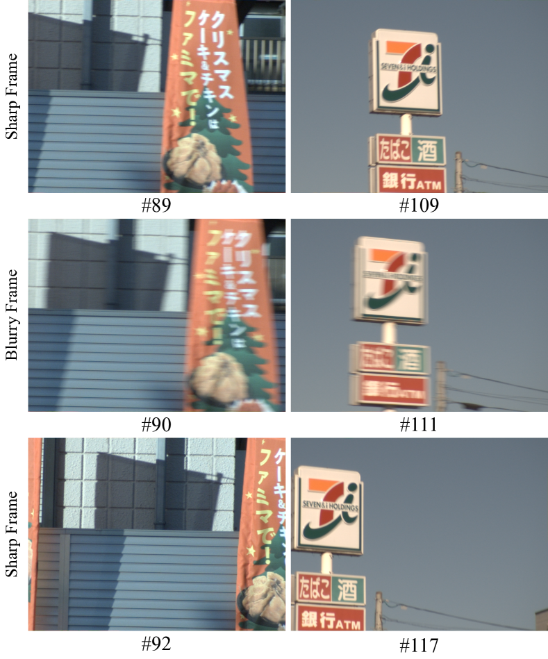
Figure 1: Examples of sharp frames observed in real-world blurry videos [1], where # denotes the frame number in a captured video. Long-term sharp features extracted from these sharp frames can be leveraged to enhance the restoration of the corresponding blurry frame.

I Introduction

With the widespread use of modern hand-held or onboard imaging devices, videos have emerged as the predominant form of media data. Due to the movement of camera or moving objects when capturing videos, blur is inevitable in many scenes, which not only leads to unpleasant visual perception but also has adverse effects on downstream applications, e.g., SLAM [2], 3D reconstruction [3] and tracking [4]. Video deblurring, aiming at recovering consecutive sharp frames, received considerable research attention in recent years [5, 6, 7, 8, 9]. Unlike single image deblurring [10, 11, 12], video deblurring methods [11, 12, 13, 14, 15, 5, 6] can leverage temporal information from adjacent blurry frames. In literature [16, 11, 17, 8], existing video deblurring methods mainly focus on the feature aggregation of adjacent blurry frames.

Due to the remarkable achievements of deep learning, extensive research has been conducted on video deblurring methods, demonstrating promising performance [11, 12, 13, 14, 15, 5, 6]. Among these methods, convolutional neural network (CNN)-based [5, 18, 19, 20, 21, 22], recurrent neural network (RNN)-based [11, 14, 7] and Transformer-based [8, 9] network architectures have been extensively investigated. Correspondingly, the strategies for feature aggregation of adjacent blurry frames can be categorized from three perspectives, i.e., explicit feature alignment and fusion based on optical flow [17, 6], temporal features propagation using recurrent states [7], and attention-based long-range feature dependency [8].

Despite advancements in deblurring performance, existing video deblurring networks are typically trained on datasets that assume consecutive blurry frames in videos and often struggle to generalize well to real-world blurry videos. However, it is a well-known fact that blur does not occur consecutively in videos. For instance, as depicted in Fig. 1, some frames in a blurry video are extremely sharp and clean, where temporal long-term sharp features are available from these sharp frames. This phenomenon arises from the dynamic variation of exposure phases when the auto-exposure function is activated [23, 24], which leads to varying amounts of blur caused by accidental camera shake or moving objects across different frames. Some relevant works have found this phenomenon [25, 6]. In [25], one deblurring model is specifically trained for a given testing video by utilizing sharp frames presented in this video as pseudo ground-truth. In [6], detected sharp frames are explicitly aligned to the current blurry frame, and the features are simply concatenated and fused in a two-stage CNN framework. Although Transformer-based model, e.g., VRT [8], is able to exploit temporal dependency of adjacent frames, long-term sharp features cannot be fully utilized, and the training and testing of VRT require a lot of resources.

In this work, we propose a video deblurring method by aggregating long-term sharp features from detected sharp frames as well as features from neighboring frames. First, a blur-aware detector is learned for distinguishing sharp frames from blurry frames. In particular, we train a blur-aware detector using a bidirectional LSTM as the backbone [6], as shown in Fig. 2. This detector enables us to identify two sharp frames for each blurry frame in both forward and backward directions. Besides cross-entropy classification loss, we introduce contrastive learning loss to improve the discrimination between sharp and blurry frames, thereby enhancing the generalization ability of our method for real-world blurry videos. Then, hybrid Transformers are adopted for aggregating features from neighboring frames and detected sharp frames. As shown in Fig. 3, a window-based local Transformer is adopted for aggregating features from neighboring frames, where the features of neighboring frames are fused with the current frame by cross-attention with shifted windows. As for detected sharp frames, a global Transformer is employed to aggregate similar long-term sharp features in a multi-scale scheme. To reduce the computational cost, global attention matrix is computed at the coarsest level. Moreover, we introduce an event fusion module into the global Transformer, thereby facilitating the extension of our method to event-based video deblurring and effectively bridging the gap between conventional video deblurring and event-driven video deblurring.

Extensive experiments have been conducted on two synthetic datasets including the GOPRO dataset [26] and REDS dataset [26], as well as one real-world BSD dataset [1] to evaluate the generalization ability of video deblurring methods on real-world blurry videos. For event-driven video deblurring, the CED dataset [27] and RBE dataset [28] are employed to assess the performance of state-of-the-art methods. By aggregating long-term sharp features, our proposed method demonstrates significant quantitative improvements over existing video deblurring methods, and there is a notable enhancement in visual quality. Our approach also exhibits higher efficiency compared to Transformer-based methods such as VRT [8]. Moreover, for event-driven video deblurring tasks, our event fusion module contributes significantly for improving performance without introducing substantial computational overhead.

The contributions of this work are three-fold:

• We propose a novel video deblurring framework that utilizes hybrid Transformers to aggregate features from both detected sharp frames and neighboring frames.

• A blur-aware detector is trained to distinguish between sharp and blurry frames, allowing us to extract long-term sharp features from detected sharp frames and facilitate the restoration of blurry ones.

• We introduce an event fusion module that extends our method to event-driven video deblurring. Extensive experiments on synthetic and real-world blurry datasets have been conducted to demonstrate the effectiveness of our approach in video deblurring as well as event-driven video deblurring.

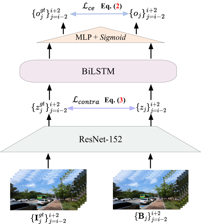
Figure 2: The architecture of the blur-aware detector is designed to distinguish between sharp and blurry frames, where a set of 5 adjacent frames, i.e., $\bm{B}_{i-2},\cdots,\bm{B}_{i},\cdots,\bm{B}_{i+2}$, are taken as input. The current frame $\bm{B}_{i}$ is then classified as either blurry or sharp. During the training process of the detector, we introduce contrastive loss Eq. (3) is introduced to enhance the discrimination between blurry and sharp frames.

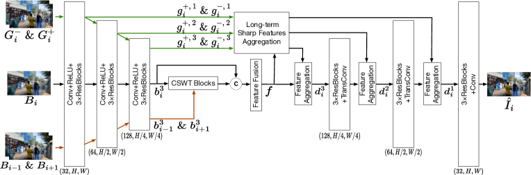
Figure 3: The flowchart of $\mathcal{F}_{\text{HybFormer}}$ for restoring a blurry frame $\bm{B}_{i}$ with its neighboring frames $\bm{B}_{i-1}$ and $\bm{B}_{i+1}$, as well as its corresponding detected sharp frames $\bm{G}_{i}^{-}\text{ and }\bm{G}_{i}^{+}$, is presented. The restoration process in $\mathcal{F}_{\text{HybFormer}}$ involves four steps: extracting features from all frames using a three-scale CNN, fusing the features of adjacent frames by window-based local Transformer, aggregating long-term sharp features using global Transformer, and finally reconstructing the latent frame $\hat{\bm{I}}_{i}$ with a decoder based on a three-scale CNN. Details regarding the window-based local Transformer and global Transformer can be found in Fig. 4 and Fig. 5, respectively.

The remainder of this paper is organized as follows. Section II briefly reviews relevant works, Section III introduces our proposed method for video deblurring as well as extension to event-driven video deblurring, Section IV presents the experimental results and ablation studies, and Section V ends this paper with concluding remarks.

II Related Work

In this section, we briefly survey relevant works including image and video deblurring, event-driven video deblurring, and Transformer-based image and video restoration methods.

II-A Image and Video Deblurring

For single image deblurring, deep learning-based methods [12, 12, 11, 29, 30, 31] have been widely studied. Tao et al. [11] proposed a scale-recurrent network in a coarse-to-fine scheme to extract multi-scale features from blurry image. Zhang et al. [30] presented a deep hierarchical multi-patch network inspired by spatial pyramid matching to handle blurry images. Ren et al. [12] adopted an asymmetric autoencoder and a fully-connected network to tackle image deblurring in a self-supervised manner. Cho et al. [13] reevaluated coarse-to-fine approach in single image deblurring and propose a fast and accurate deblurring network. Li et al. [31] proposed to adopt image quality assessment as guidance for image deblurring.

For video deblurring, Kim et al. [14] developed a spatial-temporal recurrent network with a dynamic temporal blending layer for latent frame restoration. To better leverage spatial and temporal information, Kim et al. [15] introduced an optical flow estimation step for aligning and aggregating information across the neighboring frames to restore latent clean frames. In [32], Wang et al. developed deformable convolution in a pyramid manner to implicitly align adjacent frames for better leveraging temporal information. Pan et al. [5] proposed to simultaneously estimate the optical flow and latent frames for video deblurring with the help of temporal sharpness prior. The estimated optical flow from intermediate latent frames, representing motion blur information, is fed back to the reconstruction network to generate final sharp frames. Zhong et al. [1] incorporated residual dense blocks into RNN cells to efficiently extract spatial features of the current frame. Additionally, a global spatio-temporal attention module is proposed to fuse effective hierarchical features from past and future frames, aiding in better deblurring of the current frame.

Existing video deblurring methods assume consecutively blurry frames, which is commonly inconsistent with real-world blurry videos. Shang et al. [6] found that some frames in a video with motion blur are sharp, and proposed to detect sharp frames in a video and then restore the current frame by the guidance of sharp frames. But they simply concatenate warped sharp frames and current frames for deblurring, which limits the restoration due to insufficient exploitation of sharp textures. In this work, we propose a new framework to better exploit sharp frames for video deblurring, where long-term sharp features can be aggregated by hybrid Transformers.

II-B Event-driven Video Deblurring

Event cameras [33, 34] are innovative sensors that record intensity changes in a scene at a microsecond level with slight power consumption, and have potential applications in a variety of computer vision tasks, e.g., visual tracking [35], stereo vision [36] and optical flow estimation [37]. A related research area focuses on utilizing the pure events to reconstruct high frame rate image sequences [38, 39, 40]. Recently, Pan et al. [28] formulated event-driven motion deblurring as a double integral model. Yet, the noisy hard sampling mechanism of event cameras often introduces strong accumulated noise and loss of scene details. Jiang et al. [41] proposed a sequential formulation of event-based motion deblurring, then unfolded its optimization steps as an end-to-end deep deblurring architecture. Wang et al. [42] proposed an explainable network, an event-enhanced sparse learning network (eSL-Net), to recover high-quality images from event cameras. In this work, we introduce an event fusion module to our method, bridging the gap between video deblurring and event-driven video deblurring.

II-C Transformer-based Image and Video Restoration

Recently, Transformer-based networks have shown significant performance gains in natural language and high-level vision tasks [43, 44]. As Transformer is optimized for effective representation learning and captures global interactions between contexts, it has shown promising performance in several low-level vision problems [45, 46, 47, 48]. Chen et al. [45] developed a new pre-trained model (IPT) to maximally excavate the capability of Transformer for studying the low-level computer vision task. Liang et al. [46] proposed SwinIR, a strong baseline model for image restoration based on the Swin Transformer [49] and validated its effectiveness across different low-level tasks. Yang et al. [50] proposed to use attention mechanisms to transfer high-resolution textures from reference images to low resolution images. Low resolution and reference images are formulated as queries and keys in a Transformer, respectively. Such a design encourages joint feature learning across low resolution images and reference images, enabling the discovery of deep feature correspondences through attention and accurate texture feature transfer. Zamir et al. [47] proposed an efficient Transformer model, i.e., Restormer, which incorporates key designs in the building blocks, including multi-head attention and feed-forward network, to capture long-range pixel interactions while still remaining applicable to large images. Wang et al. [48] combined a hierarchical encoder-decoder network with Transformer block forming Uformer, an effective and efficient image restoration model. Liang et al. [8] proposed a large model for video restoration with parallel frame prediction and long-range temporal dependency modeling abilities. In this work, we propose a new strategy for fusing neighboring frames and long-term sharp frames. We utilize a window-based local Transformer to fuse neighboring frames without explicit spatial alignment using optical flow. Additionally, a global Transformer is adopted for transferring sharp features from detected sharp frames, resulting in significant improvements for deblurring.

III Proposed Method

In this section, we first present our proposed video deblurring framework by aggregating long-term sharp features, then the key components including blur-aware detector and hybrid Transformers are elaborated in detail, and finally our method is extended to event-driven video deblurring by introducing an event fusion module.

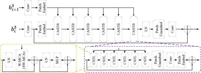
Figure 4: The architecture of CSWT Blocks $f_{\text{cswt}}$ for fusing adjacent frame features, where the third scale features $\bm{b}^{3}_{i}$ and $\bm{b}^{3}_{i+1}$ of frames $\bm{B}_{i}$ and $\bm{B}_{i+1}$ can be aggregated using cross-attention without explicit spatial alignment.

III-A Video Deblurring Framework by Aggregating Long-term Sharp Features

For an observed blurry video $\{\bm{B}_{i}\}_{i=1}^{M}$ with $M$ frames, video deblurring aims to recover consecutive sharp frames $\{\hat{\bm{I}}_{i}\}_{i=1}^{M}$. In existing video deblurring methods [17, 15, 14], a fact that sharp frames may appear in a real-world blurry video is ignored, and thus research attention is mainly paied on the feature fusion of adjacent blurry frames. As shown in Fig. 1, sharp frames usually are present near a blurry frame, and thus temporal long-term sharp features are available for facilitating the restoration of a blurry frame. It is a natural strategy to take these sharp frames as input of reconstruction network. However, there usually exists considerable temporal motion between blurry frame $\bm{B}_{i}$ and sharp frames. This phenomenon has also been investigated in [6], where optical flow-based warping network is adopted for spatial alignment of sharp and blurry frames, and the features are concatenated simply, possibly suffering from the problem of undesirable artifacts and not fully removing blur (Please see D²Nets in Figs. 6 and 7).

In this work, we propose a new video deblurring framework for aggregating long-term sharp features. For a blurry frame $\bm{B}_{i}$ with size $H\times W\times 3$, our proposed video deblurring framework for aggregating long-term sharp features can be defined as

$${\bm{G}_{i}^{+},\bm{G}_{i}^{-}} =\mathcal{F}_{\text{Detector}}(\bm{B}_{i-N},\cdots\bm{B}_{i},\cdots\bm{B}_{i+N}),$$ (1)

$$\hat{\bm{I}}_{i} =\mathcal{F}_{\text{HybFormer}}(\bm{G}_{i}^{-},\bm{B}_{i-1},\bm{B}_{i},\bm{B}_{i+1},\bm{G}_{i}^{+}),$$

where $\mathcal{F}_{\text{Detector}}$ is a blur-aware detector for finding two sharp frames $\bm{G}_{i}^{+}$ and $\bm{G}_{i}^{-}$ in adjacent $N$ frames, where the former one is in the rear direction and the latter one is in the front direction of blurry frame $\bm{B}_{i}$. When there are more than one sharp frame in the same direction, we choose the nearest sharp frame from $\bm{B}_{i}$. When there is no sharp frame in $N$ adjacent frames, $\bm{G}_{i}^{+}$ and $\bm{G}_{i}^{-}$ are simply set as $\bm{B}_{i+2}$ and $\bm{B}_{i-2}$, respectively. That is to say, for a blurry frame $\bm{B}_{i}$, we construct a set $\{\bm{G}_{i}^{-},\bm{B}_{i-1},\bm{B}_{i},\bm{B}_{i+1},\bm{G}_{i}^{+}\}$, based on which the blurry frame $\bm{B}_{i}$ can be deblurred by hybrid Transformers $\mathcal{F}_{\text{HybFormer}}$ for aggregating features from neighboring frames $\bm{B}_{i-1}$ and $\bm{B}_{i+1}$, and detected sharp frames $\bm{G}_{i}^{+}$ and $\bm{G}_{i}^{-}$. We note that detected sharp frames $\bm{G}_{i}^{+}$ and $\bm{G}_{i}^{-}$ may still have mild blur, and thus are processed in the same way. Therefore, for a blurry video $\{\bm{B}_{i}\}_{i=1}^{M}$, deblurring is conducted by processing each item in the set $\{\bm{G}_{i}^{-},\bm{B}_{i-1},\bm{B}_{i},\bm{B}_{i+1},\bm{G}_{i}^{+}\}_{i=1}^{M}$. The overall algorithm is presented in Alg. 1. Moreover, we propose an event fusion module, based on which the proposed method is easily extended to event-driven video deblurring.

III-B Detecting Sharp Frames

We treat distinguishing sharp and blurry frames in a video as a binary classification task. Following [6], we consider the temporal information in video and thus adopt bidirectional LSTM (BiLSTM) [51] to act as the classifier, by which correlations of adjacent frames in both forward and backward directions are leveraged. The architecture of BiLSTM detector is visualized in Fig. 2. For a sequence of video frames, the detector first extracts features using ResNet-152, and then transforms features to a 512-dimension vector $\{{z}_{i}\}^{M}_{i=1}$ as the input of BiLSTM, where $M$ is the total number of frames of the input video. Finally, Sigmoid function is used to normalize the outputs of BiLSTM in the range [0,1], indicating a frame is blurry or sharp.

For the consecutive frames in a blurry video $\{\bm{B}_{i}\}^{M}_{i=1}$, the output of detector is denoted by $\{{o}_{i}\}^{M}_{i=1}$, in which ${o}_{i}$ is the probability of $\bm{B}_{i}$ being a sharp frame. We binarize the outputs of BiLSTM by threshold $\epsilon=0.5$. A frame $\bm{B}_{i}$ is blurry, if $o_{i}<\epsilon$, otherwise $\bm{B}_{i}$ is sharp. Then for a given blurry frame $\bm{B}_{i}$, we can detect two sharp frames i.e., $\bm{G}_{i}^{-}$ and $\bm{G}_{i}^{+}$, from its $N$ adjacent frames in the front and rear directions, respectively. If sharp frames cannot be found, we simply set $\bm{G}_{i}^{-}$ and $\bm{G}_{i}^{+}$ as the frames $\bm{B}_{i-2}$ and $\bm{B}_{i+2}$, respectively. In this work, we empirically set the searching range $N=7$. This is because sharp frames beyond this range may have significant distinctions from the scene content in $\bm{B}_{i}$, and thus are not suitable to extract long-term sharp features.

To make the training of $\mathcal{F}_{\text{Detector}}$ easier, we split the video sequence into segments, each of which contains $5$ frames. The blur-aware detector can be trained by minimizing the binary cross-entropy loss function

$$\mathcal{L}_{\text{ce}}=-\sum_{j\in\mathbb{N}}\left(o_{j}^{gt}\log(o_{j})+(1-o_{j}^{gt})\log(1-o_{j})\right),$$ (2)

where $\mathbb{N}$ is the index set of 5 adjacent frames, ${o}_{j}^{gt}$ denotes the label of $j$-th frame, i.e., ${o}_{j}^{{gt}}=1$ when $\bm{B}_{j}$ is a sharp frame, otherwise ${o}_{j}^{{gt}}=0$. In this way, temporal information in 5 adjacent frames is considered when distinguishing sharp and blurry frames. However, we empirically find that the trained detector is not well generalized to real-world blurry videos, by only adopting the binary cross-entropy loss function. And thus, we further introduce a supervised contrastive loss function

$$\mathcal{L}_{\text{contra}}\!=\!-\log\!\left(\frac{\sum\limits_{j\in\mathbb{N}^{s}}\exp(\bm{z}_{j}\cdot\bm{z}_{j}^{gt})}{\sum\limits_{j\in\mathbb{N}^{s}}\!\!\!\exp(\bm{z}_{j}\cdot\bm{z}_{j}^{gt})+\!\!\!\!\sum\limits_{j\in\mathbb{N}^{b}}\!\!\!\exp(\bm{z}_{j}\cdot\bm{z}_{j}^{gt})}\right),$$ (3)

where $\mathbb{N}^{s}$ and $\mathbb{N}^{b}$ are subsets of $\mathbb{N}$, satisfying that $j\in\mathbb{N}^{s}$ if ${o}_{j}^{{gt}}=1$, otherwise $j\in\mathbb{N}^{b}$. Then $\bm{z}_{j}^{gt}$ denotes the feature vector of ground-truth sharp image and can be obtained by passing through the same ResNet-152 for feature extraction, and the symbol ’$\cdot$’ denotes the normalized inner dot product. Benefiting from contrastive loss $\mathcal{L}_{\text{contra}}$, the features between sharp and blurry frames are forced to be as distinguishable as possible, leading to better generalization ability on real-world blurry videos.

Finally, the total loss function for training $\mathcal{F}_{\text{Detector}}$ is defined as

$$\mathcal{L}_{\text{Dector}}=\mathcal{L}_{\text{ce}}+\lambda\mathcal{L}_{\text{contra}},$$ (4)

where $\lambda$ is a hyper-parameter and is set $\lambda=10$ in all the experiments.

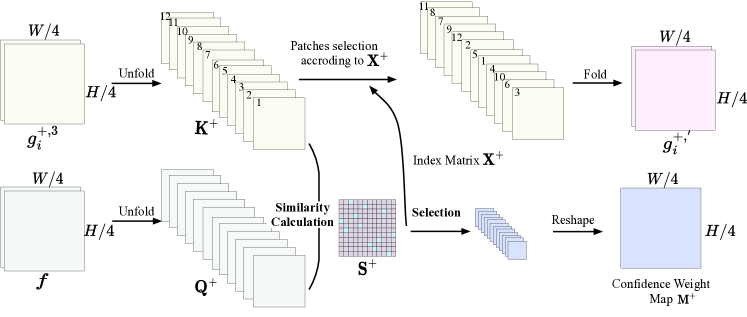
Figure 5: Global attention of long-term sharp feature $\bm{g}^{+,3}_{i}$ in rear frame $\bm{G}^{+}_{i}$ and feature $\bm{f}$ in the third scale. The global similarity for each coordinate is recorded in $\bm{S}^{+}$, enabling identification of the most relevant patches in the index matrix $\bm{X}^{+}$ along with their corresponding confidence map $\bm{M}^{+}$. These patches are then folded into a new feature representation denoted as $\bm{g}_{i}^{+,^{\prime}}$. Similarly, the long-term sharp features $\bm{g}_{i}^{-,3}$ from the front frame $\bm{G}_{i}^{-}$ can be processed in the same way.

III-C Video Deblurring via Hybrid Transformers

The hybrid Transformer $\mathcal{F}_{\text{HybFormer}}$ mainly consists of two key components, i.e., window-based local Transformer for aggregating features from neighboring frames $\bm{B}_{i-1}$ and $\bm{B}_{i+1}$, and global Transformer for aggregating long-term sharp features from detected sharp frames $\bm{G}_{i}^{+}$ and $\bm{G}_{i}^{-}$. As shown in Fig. 3, hybrid Transformers are implemented in the feature space extracted by CNN. In particular, a three-scale CNN encoder is adopted for feature extraction, where an input frame with size $H\times W\times 3$ is transferred to features with three scales $H\times W\times C$, $\frac{H}{2}\times\frac{W}{2}\times 2C$, and $\frac{H}{4}\times\frac{W}{4}\times 4C$, where $C$ is channel number and we set $C=32$. The window-based local Transformer is implemented in the third scale, while global Transformer is implemented in multi-scale scheme. Finally, the aggregated features are reconstructed to deblurred frames in a corresponding three-scale CNN decoder.

As for learning the parameters of $\mathcal{F}_{\text{HybFormer}}$, we adopt $\ell_{1}$-norm loss function

$$\mathcal{L}_{\text{HybFormer}}\!=\!\left\|\mathcal{F}_{\text{HybFormer}}(\bm{G}_{i}^{-},\bm{B}_{i-1},\bm{B}_{i},\bm{B}_{i+1},\bm{G}_{i}^{+})\!-\!\bm{I}_{i}^{gt}\right\|_{1}.$$ (5)

III-C1 Window-based Local Transformer for Aggregating Neighboring Frames

As shown in Fig. 4, we adopt cross-attention shifted window Transformer (CSWT) blocks $\bm{f}_{\text{cswt}}$ to fuse current frame $\bm{B}_{i}$ and its two neighboring frames $\bm{B}_{i-1}$ and $\bm{B}_{i+1}$, which is implemented in the third scale.

We take the feature aggregation of $\bm{B}_{i}$ and $\bm{B}_{i+1}$ as example, and $\bm{B}_{i-1}$ can be processed in the same way. Let $\bm{b}_{i}^{3}$ and $\bm{b}_{i+1}^{3}$ be the features of $\bm{B}_{i}$ and $\bm{B}_{i+1}$ in third scale with size ${\frac{H}{4}\times\frac{W}{4}\times 16C}$. The key idea of window-based local Transformer $f_{\text{cswt}}$ is cross-attention without spatial alignment, where the features extracted from $\bm{b}_{i}^{3}$ as $Key$ and $Value$ matrices, and features extracted from $\bm{b}_{i+1}^{3}$ as $Query$ matrices. The architecture of $f_{\text{cswt}}$ is borrowed from [46, 49], and self-attention is modified to cross-attention for integrating adjacent frames. The architecture of $\bm{f}_{\text{cswt}}$ can be seen in Fig. 4. Following the setting in SwinIR [46], there are 6 Cross-Attention Swin Transformer Blocks (CASTB) in $\bm{f}_{\text{cswt}}$. Each CASTB contains 6 Cross Swin Transformer Layers (CSTL) and 1 convolutional layer. For each CSTL, it includes a LayerNorm(LN), W-MCA or SW-MCA and MLP, where W-MCA and SW-MCA denote window based multi-head cross-attention using regular and shifted window partitioning configurations, respectively. W-MCA and SW-MCA alternate in each CSTL, which maintain the efficient computation of non-overlapping windows and improve modeling power, as described in [49]. The number of attention heads is 8.

Then, the features from two neighboring frames can be aggregated as

$$\bm{b}^{\prime}_{i-1} =f_{\text{cswt}}\left(\bm{b}_{i}^{3},\bm{b}_{i-1}^{3}\right),$$ (6)

$$\bm{b}^{\prime}_{i+1} =f_{\text{cswt}}\left(\bm{b}_{i}^{3},\bm{b}_{i+1}^{3}\right),$$

$$\bm{f} ={conv}(\mathcal{C}(\bm{b}^{\prime}_{i-1},\bm{b}_{i}^{3},\bm{b}^{\prime}_{i+1})),$$

where $\mathcal{C}$ is concatenation, and $conv$ is a convolutional layer. We fed the concatenation of $\bm{b}_{i}^{3},\bm{b}^{\prime}_{i-1}\text{ and }\bm{b}^{\prime}_{i+1}$ into a convolutional layer to get new features $\bm{f}$ which integrates current and neighboring frame for reconstructing deblurred frame in decoder.

Algorithm 1 Aggregating Sharp Features for Video Deblurring

0:  Blurry video with $M$ frames $\{\bm{B}_{i}\}_{i=1}^{M}$

0:  Deblurring video $\{\hat{\bm{I}}_{i}\}_{i=1}^{M}$

1:  Distinguishing sharp and blurry frames using $\mathcal{F}_{\text{Detector}}$.

2:  Constructing a set $\{\bm{G}_{i}^{-},\bm{B}_{i-1},\bm{B}_{i},\bm{B}_{i+1},\bm{G}_{i}^{+}\}_{i=1}^{M}$, where $\bm{G}_{i}^{-}\text{ and }\bm{G}_{i}^{+}$ are detected sharp frames of $\bm{B}_{i}$ in the front and rear directions.

3:  for  $i=1:M$  do

4:     $\hat{\bm{I}}_{i}=\mathcal{F}_{\text{HybFormer}}(\bm{G}_{i}^{-},\bm{B}_{i-1},\bm{B}_{i},\bm{B}_{i+1},\bm{G}_{i}^{+}).$

5:  end for

6:  return  Deblurring video frames $\{\hat{\bm{I}}_{i}\}_{i=1}^{M}$

III-C2 Global Transformer for Aggregating Sharp Frames

Considering the temporal motion between current current frame and detected sharp frames, we propose to utilize global attention across current frame and sharp frames to measure the similarity for each coordinate. The key idea of global Transformer includes a matching operation for calculating relevance between current frame and sharp frames, and a selection operation for picking out the most relevant long-term sharp information to the current frame. We take the aggregation of long-term features from rear sharp frame $\bm{G}_{i}^{+}$ as an example to show how to compute global attention.

Global Attention for Aggregating Long-term Sharp Features. We need to compute the global similarity between feature $\bm{f}$ and the feature $\bm{g}_{i}^{+}$ of detected sharp frame $\bm{G}_{i}^{+}$. By taking $\bm{g}_{i}^{+,3}$ in third scale as an example, we show how to compute the global similarity. The features $\bm{f}$ and $\bm{g}_{i}^{+,3}$ are unfolded into patches to form $Query$ matrix $\bm{Q}^{+}$ with size $\frac{HW}{16}\times p^{2}$ and $Key$ matrix $\bm{K}^{+}$ with size $p^{2}\times\frac{HW}{16}$, and we normalize $\bm{Q}^{+}$ and $\bm{K}^{+}$ to obtain the similarity matrix $\bm{S}^{+}=\bm{Q}^{+}\times\bm{K}^{+}$ with size $\frac{HW}{16}\times\frac{HW}{16}$, whose element measures the similarity between extracted patches.

For a patch $i$, the most relevant patch in sharp feature can be found by $\bm{X}^{+}(i)=\arg\underset{}{\max}\bm{S}^{+}(i,:)$ as well as confidence weight map $\bm{M}^{+}(i)=\underset{}{\max}\bm{S}^{+}(i,:)$, where $\bm{M}^{+}$ and $\bm{X}^{+}$ with size $\frac{HW}{16}\times 1$ are the index to the most similar patches and the confidence weight map. Then, $\bm{M}^{+}$ and $\bm{X}^{+}$ can be reshaped to matrices with size $\frac{H}{4}\times\frac{W}{4}$, having the same dimension with features in third scale.

Next, we can get the sharp features that are most related to the current frame patch according to index matrix $\bm{X}^{+}$ and fold these patches together, which is the reverse operation of the unfolding operation to get new features $\bm{g}_{{i}}^{+,^{\prime}}$. Instead of directly applying the confidence weight map $\bm{M}^{+}$ to $\bm{g}_{i}^{+,3}$, we first fuse the sharp texture features $\bm{g}_{i}^{+,3}$ from detected sharp frame with features $\bm{f}$ to leverage more information. Such fused features are further element-wisely multiplied by the confidence weight map $\bm{M}^{+}$ and added back to $\bm{f}$ to get the final intput of $f_{\text{dec}}$. This step can be represented as

$$\bm{g}_{i}^{+,}\prime=f_{\text{fold}}(\bm{g}_{{i}}^{+,3};\bm{X}^{+}),$$

$$\bm{g}_{i}^{-,}\prime=f_{\text{fold}}(\bm{g}_{{i}}^{-,3};\bm{X}^{-}),$$

$${\bm{d}}_{i}^{3}\!=\!conv\left(\mathcal{C}(\bm{g}_{i}^{+,}\prime,\bm{f})\right)\!\odot\!\bm{M}^{+}\!\!\!+conv\left(\mathcal{C}(\bm{g}_{i}^{-,}\prime,\bm{f})\right)\!\odot\!\bm{M}^{-}\!\!\!+\!\bm{f},$$ (7)

where $f_{\text{fold}}$ denotes searching most relevant patches according to index $\bm{X}^{+}$ to get folded new features $\bm{g}_{{i}}^{+,^{\prime}}$, and $\odot$ denotes element-wise multiplication. And the features $\bm{g}_{i}^{-,^{\prime}}$ from front sharp frame $\bm{G}_{i}^{-}$ can be handled in the same way. Finally, the long-term sharp features can be aggregated with feature $\bm{f}$, where confidence maps $\bm{M}^{+}$ and $\bm{M}^{-}$ are considered when aggregating features.

Implementation in Multi-scale Scheme. To fully exploit long-term sharp features, feature aggregation is performed in the multi-scale scheme, where features in first and second scales $\bm{g}^{+,2}_{i}$ and $\bm{g}^{+,1}_{i}$ are also aggregated. Due to the computational cost of global attention, we do not suggest to directly compute index matrix $\bm{X}^{+}$ and confidence map $\bm{M}^{+}$ in the first and second scales. As for the confidence map $\bm{M}^{+}$, it can be upsampled with corresponding factor. And for index matrix $\bm{X}^{+}$, we need to keep the same dimension for unfolded feature tensors in first and second scales. Therefore, to ensure the applicability of $\bm{X}^{+}$ at different scales, we adjusted the parameters of unfolding operation at different scales to ensure that the total numbers of unfolding patches in three scales are consistent.

Recalling that the spatial size of $\bm{X}^{+}$ is $\frac{H}{4}\times\frac{W}{4}$, i.e., the total number of extracted patches is $L=\frac{H}{4}\times\frac{W}{4}$. Therefore, we need to keep the same number for the other two scales. We have got the long-term features in three-scale CNN, i.e., $\bm{g}_{{i}}^{+,1}$, $\bm{g}_{{i}}^{+,2}$ and $\bm{g}_{{i}}^{+,3}$, whose spatial sizes are $H\times W$, $\frac{H}{2}\times\frac{W}{2}$ and $\frac{H}{4}\times\frac{W}{4}$. Unfolding operation aims to extract sliding local patches from a batched input tensor. The total number of sliding window patches is

$$L=\prod_{x\in\{h,w\}}\left\lceil\frac{x+2\times p-(k-1)}{r}\right\rceil$$ (8)

where $\lceil\cdot\rceil$ is the ceiling operation, $h$ and $w$ are height and width of features, and ${p}$, ${k}$, ${r}$ denote the padding size, patch size and stride size, respectively. To satisfy the condition $L=\frac{H}{4}\times\frac{W}{4}$, we set the parameters $\{[h,w],[k,k],[p,p],[r,r]\}$ for the features $\bm{g}_{i}^{+,3}$, $\bm{g}_{i}^{+,2}$, $\bm{g}_{i}^{+,1}$ in three scales respectively as $\{[\frac{H}{4},\frac{W}{4}],[3,3],[1,1],[1,1]\}$, $\{[\frac{H}{2},\frac{W}{2}],[6,6],[2,2],[2,2]\}$, $\{[{H},{W}],[12,12],[4,4],[4,4]\}$. And the features $\bm{g}^{-}_{i}$ share the same setting. In addition, the center spatial position of the same patch with different scales keeps unchanged, guaranteeing that the confidence weight map $\bm{M}$ can be upsampled for different scales by bilinear interpolation.

Then, the feature aggregation in the second scale can be defined as

$$\bm{d}\prime=f_{\text{dec}}({\bm{d}_{i}^{3}}),$$

$$\bm{g}_{i}^{+,}\prime=f_{\text{fold}}(\bm{g}_{{i}}^{+,2};\bm{X}^{+}),$$

$$\bm{g}_{i}^{-,}\prime=f_{\text{fold}}(\bm{g}_{{i}}^{-,2};\bm{X}^{-}),$$

$$\footnotesize{\bm{d}_{i}^{2}\!=\!conv\!\left(\mathcal{C}(\bm{g}_{i}^{+,}\prime,\bm{d}\prime)\right)\!\odot\!\bm{M}^{+}\!\!\uparrow\!\!+conv\!\left(\mathcal{C}(\bm{g}_{i}^{-,}\prime,\bm{d}\prime)\right)\!\odot\!\bm{M}^{-}\!\!\uparrow\!\!+\!\bm{d}\prime},$$ (9)

where $f_{\text{dec}}$ is one layer in decoder, consisting of three ResBlocks and one transposed convolution, and the feature and confidence map are upsampled with factor 2. The aggregation in the scale 1 shares similar steps, where the feature $\bm{d}_{i}^{1}$ is with size $H\times W\times C$ and is finally mapped to deblurred frame $\hat{\bm{I}}_{i}$ with size $H\times W\times 3$ using three ResBlocks and one convolutional layer.

III-D Extension to Event-driven Video Deblurring

We take one step further to leverage events in $\mathcal{F}_{\text{HybFormer}}$ for event-driven deblurring [40]. For an event camera, given a blurry frame $\bm{B}_{i}$, its corresponding stream of events $\bm{E}_{i}$ are available. Each event has the form $\mathbf{(}t,x,y,p)$, which records intensity changes for coordinates $\mathbf{(}x,y)$ at time ${t}$, and polarity $p=\pm 1$ denotes the increase or decrease of intensity change. In this work, we transform the events stream into a tensor with 40 channels for each frame as in [42]. We introduce an event fusion module to incorporate events into frame features for event-driven deblurring. Our event fusion module transfers the event $\bm{E}_{i}$ to feature $\bm{e}$ through 5 convolution layers, having the same size as $\bm{f}$. Event feature $\bm{e}$ can be upsampled for different scales by bilinear interpolation. Then an fusion module is implemented by calculating a reweighting map through cross-attention between event feature and frame feature, which can be used to facilitate deblurring by matrix multiplication with the features of frames.

IV Experiments

In this section, we evaluate our proposed method on five benchmark datasets, including GOPRO [26], REDS [26] and BSD [1] datasets for video deblurring, and RBE [28] and CED [27] datasets for event-driven video deblurring. And we conduct ablation study to verify the key contributions of our proposed method on GOPRO dataset. As for state-of-the-art competing deblurring methods, we take both image deblurring and video deblurring methods into comparison, where image deblurring methods include DMPHN [30] and MIMO-UNet++ [13], and video deblurring methods include STFAN [52], ESTRNN [1], CDVD-TSPNL [17], VRT [8] and D²Nets [6]. As for event-driven deblurring methods, we take BHA [28], eSL-Net [42], eSL-Net++[53] and D²Nets* [6] into comparison. Finally, we validate their generalization performance on real-world blurry videos. More video results can be found from the link.

IV-A Datasets and Training Details

IV-A1 Datasets

For video deblurring, three datasets are adopted for evaluation, where GOPRO and REDS are synthetic datasets, while BSD dataset contains real-world blurry videos. For event-driven video deblurring, synthetic blurry dataset CED and real-world blurry dataset RBE are adopted.

GOPRO Dataset: GOPRO dataset [26] is widely adopted for image and video deblurring. The videos in the original GOPRO dataset are with framerate of 240 FPS. We follow [26] to split the training and testing sets. To satisfy the condition that sharp frames exist in a blurry video, we generate non-consecutively blurry frames in a video by randomly averaging adjacent sharp frames, i.e., the average number is randomly chosen from 1 to 15. And we classify that a generated frame $\bm{B}_{i}$ is sharp if the number of averaging frames is smaller than 5, i.e., $o_{i}^{gt}=1$, otherwise $o_{i}^{gt}=0$. It is worth noting that we randomly generate 50$\%$ blurry frames in a video, while the other 50$\%$ frames are sharp, without constraining that there must be 2 sharp ones in consecutive 7 frames.

REDS Dataset: Another widely used dataset is REDS dataset [26], and there are 240 videos for training, 30 videos for testing. We generate non-consecutively blurry frames in a similar way as GOPRO. When the framerate is not high enough, simply averaging frames may generate unnatural spikes or steps in the blur trajectory [26], especially when the resolution is high and the motion is fast. Hence, we employed FLAVR [54] to interpolate frames, increasing the framerate to virtual 960 FPS by recursively interpolating the frames. Thus, we can synthesize frames with more severe degrees of blur, i.e., the average number is randomly chosen from 3 to 39. And we classify that a generated frame $\bm{B}_{i}$ is sharp if the number of averaging frames is smaller than 17, i.e., $o_{i}^{gt}=1$, otherwise $o_{i}^{gt}=0$.

BSD Dataset: Zhong et al. [1] provided a real-world blurry video dataset by using a beam splitter system [55] with two synchronized cameras. By controlling the length of exposure time and strength of exposure intensity when capturing videos, the system could obtain a pair of sharp and blurry video samples by shooting videos at the same time. They collected blurry and sharp video sequences for three different blur intensity settings, i.e., sharp exposure time – blurry exposure time are set as 1ms–8ms, 2ms–16ms and 3ms–24ms, respectively. We note that blurry videos in BSD dataset, especially for long exposure time, suffer from severe blur, but sharp frames still are present to provide long-term sharp features. The testing set has 20 video sequences with 150 frames in each intensity setting. We use these testing sets for evaluating generalization ability.

CED Dataset: Scheerlinck et al. [27] presented the first Color Event Camera Dataset (CED) by color event camera ColorDAVIS346, containing 50 minutes of footage with both color frames and events. We also employed FLAVR[54] to interpolate frames for generating blurry frames as the same with REDS. We randomly split the sequences in CED into training, validation and testing sets, and report the corresponding comparison results against the state-of-the-art models by retraining them with the same setting.

RBE Dataset: Pan et al. [28] presented a real blurry event dataset, where each real sequence is captured with the DAVIS under different conditions, such as indoor, outdoor scenery, low lighting conditions, and different motion patterns (e.g., camera shake, objects motion) that naturally introduce motion blur into the APS intensity images. There is no ground-truth data available on this dataset. Hence, we only use it for qualitative comparison.

TABLE I: Quantitative comparison of deblurring results of on GoPro dataset.

Method	DMPHN[30]	STFAN[52]	ESTRNN[1]	MIMO-UNet++[13]	D2Nets[6]	CDVD-TSPNL[17]	VRT[8]	Ours
PSNR	32.09	31.76	33.52	35.49	35.18	36.65	37.02	37.33
SSIM	0.897	0.873	0.912	0.938	0.943	0.958	0.961	0.962

TABLE II: Quantitative comparison of deblurring results on REDS dataset.

Method	DMPHN[30]	STFAN[52]	ESTRNN[1]	MIMO-UNet++[13]	D2Nets[6]	CDVD-TSPNL[17]	VRT[8]	Ours
PSNR	37.62	38.09	38.38	39.05	38.82	40.06	40.84	41.45
SSIM	0.956	0.959	0.962	0.965	0.969	0.977	0.981	0.982

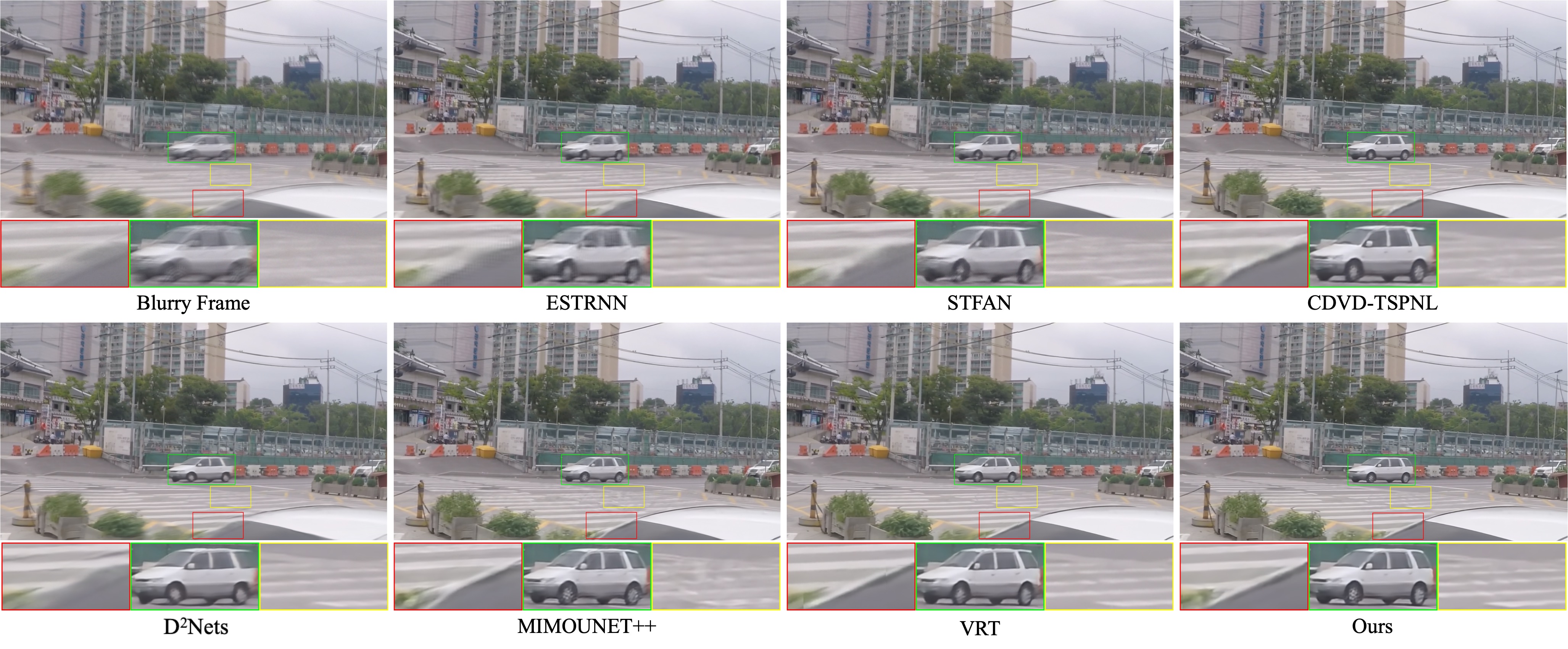
Figure 6: Visual comparison of deblurring results on GOPRO dataset [26].

IV-A2 Training Details

In the training process, we use ADAM optimizer [56] with parameters $\beta_{1}=0.9$, $\beta_{2}=0.999$, and $\epsilon=10^{-8}$ for all the networks in $\mathcal{F}_{\text{Detector}}$ and $\mathcal{F}_{\text{HybFormer}}$. The batch size is 12 and patch size is set as 200 $\times$ 200. The learning rates for reconstruction network $\mathcal{F}_{\text{HybFormer}}$ is initialized to be $1\times 10^{-4}$ and is decreased by multiplying 0.5 after every 200 epochs. The training ends after 500 epochs. For BiLSTM detector $\mathcal{F}_{\text{Detector}}$, the learning rate is set to be $1\times 10^{-4}$, and the training ends after 20 epochs.

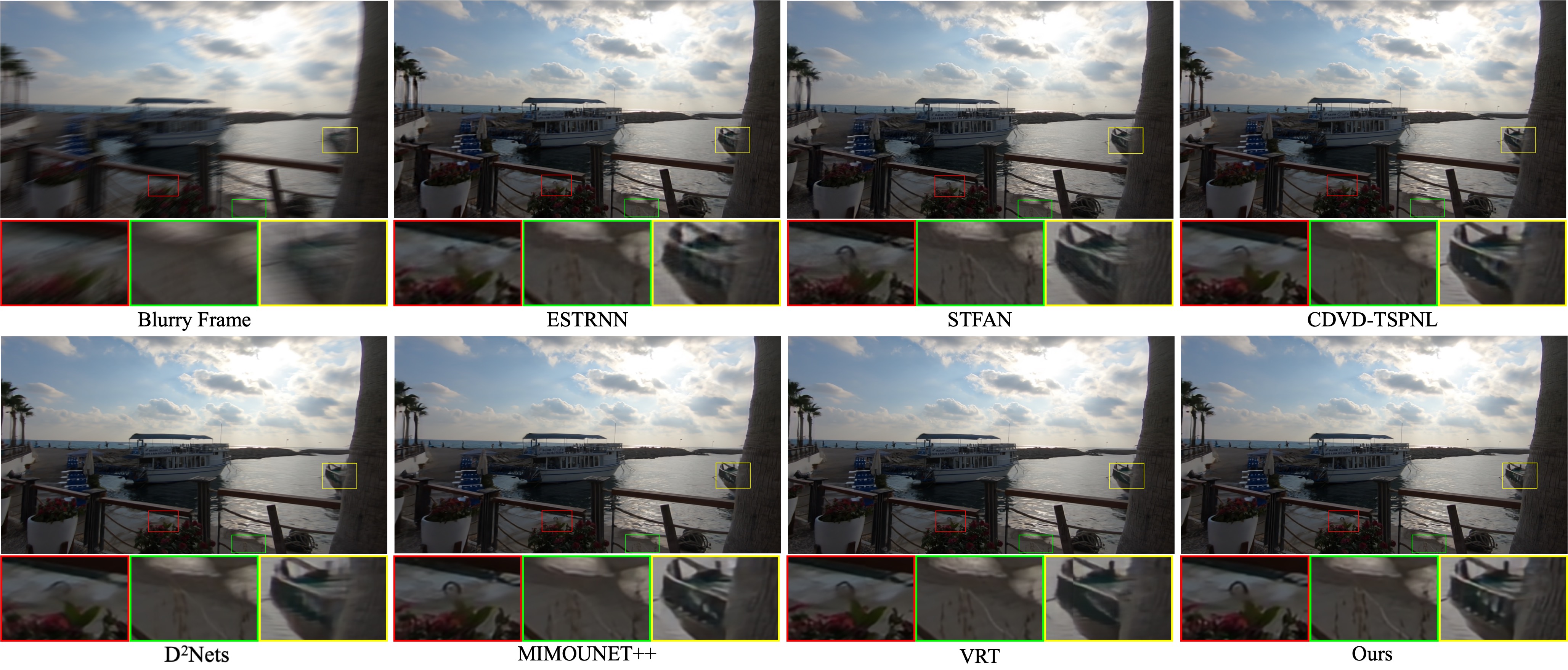
Figure 7: Qualitative comparison on REDS dataset[26].

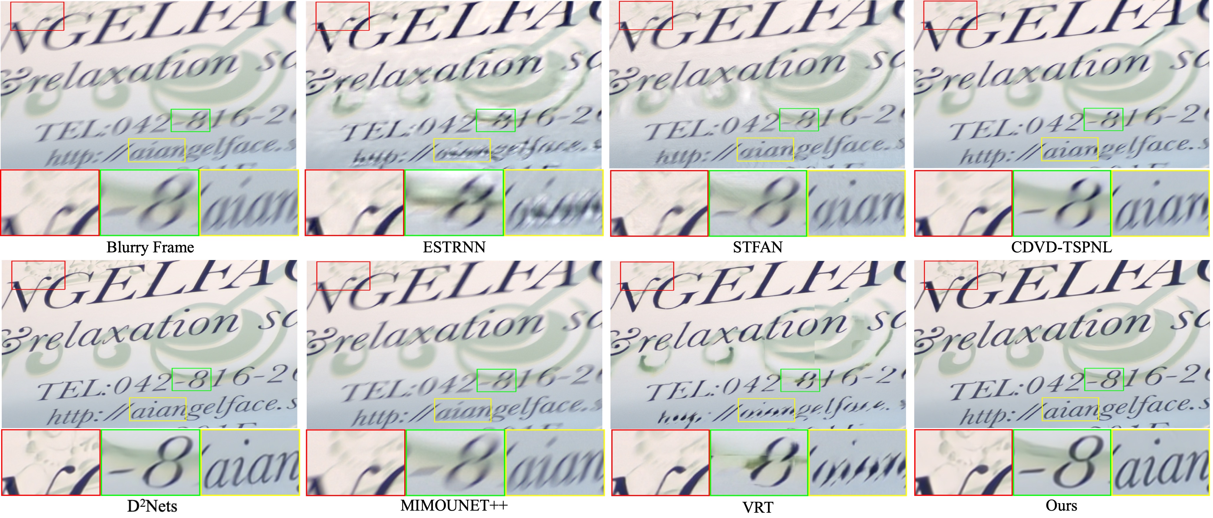
Figure 8: Visual comparison of deblurring results on real-world blurry video [1].

TABLE III: Comparison of efficiency and model size. The experiment was conducted on GeForce RTX 3090 with videos (240 $\times$ 240).

Method	Params(M)	GFLOPs	Runtime(s)
DMPHN[30]	21.70	189.3	0.058
STFAN[52]	5.37	202.9	0.150
ESTRNN[1]	2.47	11.2	0.035
MIMO-UNet++[13]	16.11	135.6	0.022
D2Nets[6]	32.54	326.4	0.131
CDVD-TSPNL[17]	5.50	1343.9	0.251
VRT[8]	35.60	3229.7	0.898
Ours	30.63	342.6	0.107

IV-B Evaluation on Video Deblurring

Two synthetic datasets GOPRO and REDS are employed for quantitative and qualitative evaluation as well as computational efficiency, and one real-world dataset BSD is adopted for evaluating generalization ability.

IV-B1 Comparison on Synthetic Datasets

When synthesizing blurry frames in GOPRO and REDS, more frames are averaged in REDS, thus resulting in more severe blur in REDS than in GOPRO.

Evaluation on GOPRO Dataset. We retrain all these competing methods except VRT on the training set of GOPRO for a fair comparison. For Transformer-based method VRT, we finetune the model provided by authors on our dataset. It is worth noting that VRT is trained on Tesla A100 GPUs, but we do not have such large computing resources. Hence, we use a smaller patch size for finetuning. Table I reports the comparison of PSNR and SSIM metrics for the competing methods. One can see that our method outperforms CNN-based and RNN-based methods by a large margin, among which D²Nets [6] also leverages sharp frames similar to our method. Benefiting from long-term sharp features, our method and D²Nets are generally better than other CNN-based methods. However, in D²Nets, optical flow is adopted to perform spatial alignment, possibly yielding texture loss and deformation artifacts. And thus, our method is still much better than D²Nets.

In comparison to Transformer-based method VRT, the attention in temporal dimension can implicitly benefit from the long-term sharp features, and thus VRT is also notably better than CNN-based methods. Our method still achieves about 0.2dB PSNR gain than VRT. Meanwhile, our method is much more efficient than VRT, as shown in Table. III, although their parameters are similar. Considering the quantitative performance in Table I and computational cost in Table III, our method has a good tradeoff between computational cost and performance.

In terms of visual quality comparison in Fig. 6, flow-based method, e.g., CDVD-TSPNL and RNN-based methods, e.g., STFAN and ESTRNN, all fail in recovering sharp texture. MIMOUNet++ is an image deblurring method, and it has a better deblurring result, but it produces some undesirable artifacts, referring to yellow box in Fig. 6. D²Nets utilizes sharp frames by using optical flow for warping sharp frames to current frame, and then directly concatenating them with current frame. However, direct concatenation can not fully extract sharp textures for reconstructing current blurry frame. Our method can achieve sharper texture details by utilizing useful sharp information searched from detected sharp frames by global Transformer in the multi-scale scheme, and the boundary outline of the car is quite clearer than the results by the competing methods in Fig. 6.

Evaluation on REDS Dataset. The CNN-based and RNN-based methods are also retrained on the REDS dataset, and VRT is finetuned by adopting a similar setting with GOPRO dataset. The quantitative results are reported in Table II. Benefiting from attention mechanism, VRT and our method are much better than the other methods, because long-term sharp features can be exploited in these methods. Among them, our method achieves the best performance in comparison with competing methods in terms of both PSNR and SSIM. Fig. 7 shows the visual quality comparison, from which one can see that our method can recover sharper texture details, due to the guidance of long-term sharp features, while the results by other methods still suffer from mild blur or over-smoothing textures. From Fig. 7, one can see unsatisfactory distortion of the street lamp post in the red box of VRT [8] and the details of fences in yellow box are not clear.

IV-B2 Generalization Evaluation on Real-world BSD Dataset

We evaluate generalization ability of these methods on real-world blurry videos, where the models of competing methods trained on REDS dataset are applied to handle real-world blurry videos from BSD dataset. For the comparison, we adopt two settings. First, we use our blur-aware detector to find sharp frames in BSD testing dataset, and we select videos that contain more than 40$\%$ sharp frames as real non-consecutively blurry videos to satisfy the condition of long-term sharp features. We obtain 13 non-consecutively blurry videos from BSD dataset for evaluating generalization ability, and we denote it as BSD^-. The results are reported in Table IV. Second, we adopt all the testing videos from BSD for evaluation, and the results are reported in Table V. In this setting, there are videos without sharp frames, i.e., $\bm{G}_{i}^{+}$ and $\bm{G}_{i}^{-}$ cannot be found by detector, and we use $\bm{B}_{i-2}$ and $\bm{B}_{i+2}$ to substitute $\bm{G}_{i}^{-}$ and $\bm{G}_{i}^{+}$, respectively.

As shown in Table IV, our method achieves the highest PSNR and SSIM values, indicating better generalization ability of our method. We note that VRT is much inferior to our method, although it achieves comparable metrics on GOPRO dataset in Table I and REDS dataset in Table II. This may be attributed that VRT is overfitted to the training set, resulting in poor generalization ability. In Table V, the results for different capturing settings are reported, where our method achieves the highest PSNR and SSIM metrics for all the three settings. We note that our method still works well for real-world videos without sharp frames, making our method applicable in practical applications. Also Transformer-based method VRT has the worst generalization ability. As shown in Fig. 8, our method achieves the most visually plausible deblurring results with sharper textures, while STFAN, VRT, ESTRNN and MIMOUNet++ cannot fully remove severe blur. CDVD-TSPNL and D²Nets generate undesirable artifacts on letters in red box.

TABLE IV: Quantitative comparison of generalization ability on BSD^- dataset.

Method	DMPHN[30]	STFAN[52]	ESTRNN[1]	MIMO-UNet++[13]	D2Nets[6]	CDVD-TSPNL[17]	VRT[8]	Ours
PSNR	30.39	27.69	25.984	28.77	30.58	28.79	26.73	32.10
SSIM	0.924	0.860	0.843	0.884	0.933	0.900	0.870	0.937

TABLE V: Quantitative comparison of generalization ability on the whole BSD dataset.

Method	1ms–8ms	2ms–16ms	3ms–24ms
DMPHN[30]	29.94/0.905	28.47/0.885	27.64/0.877
STFAN[52]	27.49/0.845	25.71/0.799	26.17/0.825
ESTRNN[1]	26.32/0.827	24.36/0.779	25.29/0.803
MIMO-UNet++[13]	29.27/0.874	26.98/0.830	27.40/0.850
D2Nets[6]	30.14/0.911	28.55/0.888	28.40/0.891
CDVD-TSPNL[17]	28.16/0.870	26.37/0.835	26.78/0.851
VRT[8]	25.99/0.845	23.67/0.785	25.07/0.822
Ours	31.40/0.918	29.93/0.895	29.25/0.891

IV-C Evaluation on Event-Driven Video Deblurring

Our method is trained on CED dataset, dubbed Ours*. As for the competing methods, D²Nets* is also re-trained on CED dataset, while the models of eSL-Net [42] and eSL-Net++ [53] provided by the authors are directly adopted for evaluation since their training codes are not available. As shown in Table VI, one can see our method can achieve higher PSNR and SSIM values than the other methods. eSL-Net [42] is very dependent on the number of utilized events. More events will lead to darkness, and fewer events will lead to not removing blur. Form Fig. 9, event-based method eSL-Net [42] generated unpleasurable darkness noise. The results by eSL-Net++ [53] still suffer from slight blur. And D²Nets* [6] can remove much blur but the restored details are limited due to the simple utilization of adjacent frames and events. The hands and shoes are blurry in the results of D²Nets* in Fig. 9. One can see our method can achieve better results compared with eSL-Net++ and D²Nets*.

In addition, we also compare our method with the other methods on RBE dataset [28]. The models of D²Nets* [6] and our method trained on CED dataset are adopted for testing. For BHA [28] and eSL-Net++ [53], we use the pre-trained models provided by authors, since they do not release training codes. In Fig. 10, one can see eSL-Net++ fail to deblur on real blurry frames. BHA and D²Nets* can remove the blur but suffer from noises and darkness artifacts, while our method can achieve more visually plausible deblurring results compared with the other methods.

TABLE VI: Quantitative comparison of deblurring results on CED dataset.

Method	eSL-Net [42]	eSL-Net++[53]	D2Nets*[6]	Ours*
PSNR	23.12	25.797	31.72	33.55
SSIM	0.716	0.7545	0.912	0.936

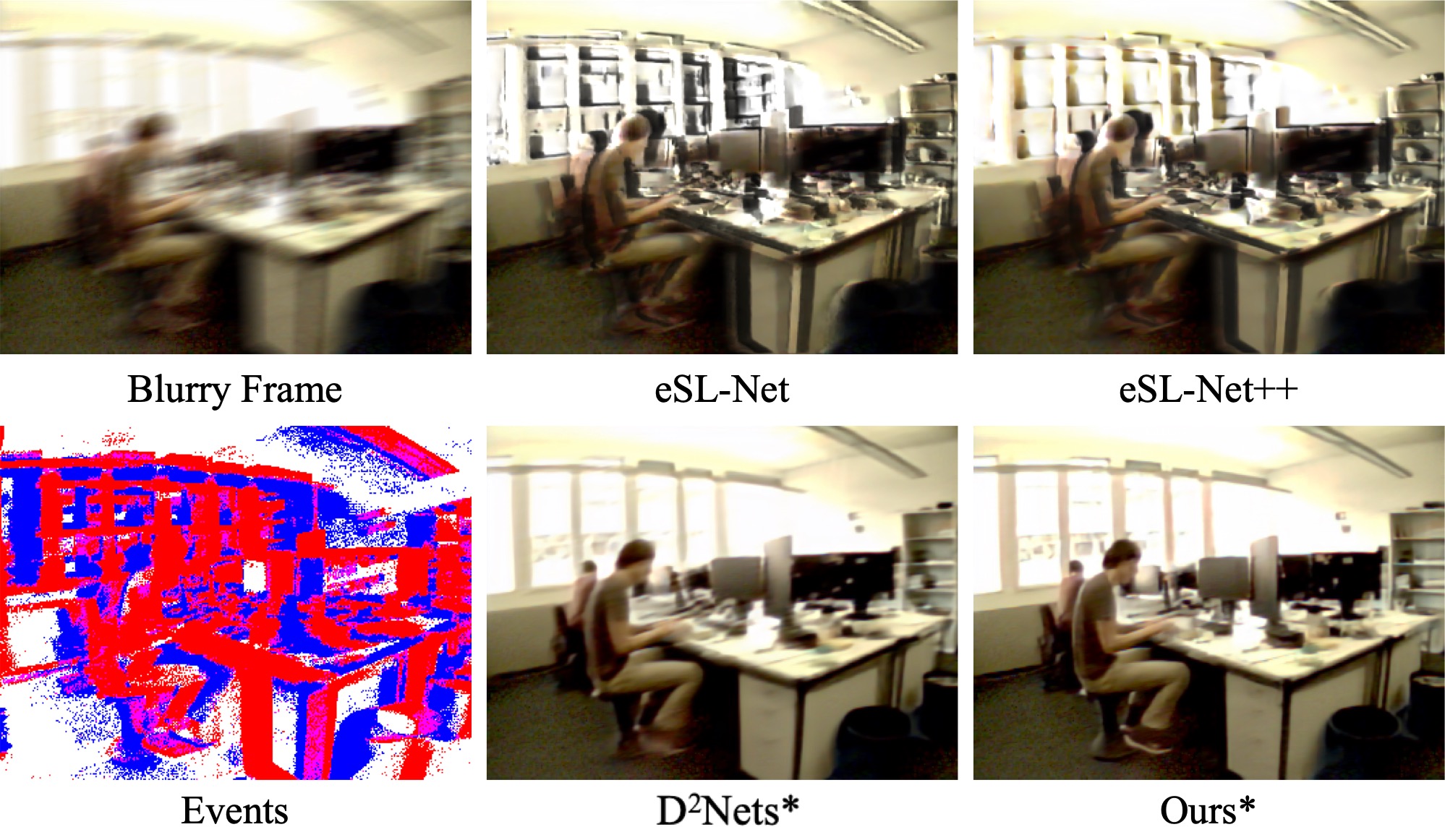
Figure 9: Visual comparison of deblurring results on CED dataset. Please zoom in for better view.

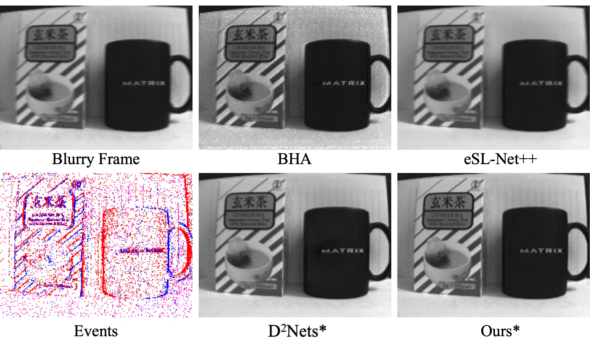
Figure 10: Visual comparison of deblurring results on RBE dataset. Please zoom in for better view.

IV-D Ablation Study

TABLE VII: The accuracy of BiLSTM detector by using different loss.

Loss	Only $\mathcal{L}_{\text{ce}}$	$\mathcal{L}_{\text{ce}}$&$\mathcal{L}_{\text{contra}}$
GOPRO [26]	99.9$\%$	98.4$\%$
REDS [26]	87.2$\%$	87.2$\%$
Generalization	90.5$\%$	95.0$\%$

TABLE VIII: Component analysis on the GOPRO dataset.

Self-attention	Cross-attention	Global attention	PSNR	SSIM
✓	✗	✗	35.28	0.938
✓	✗	✓	36.24	0.953
✗	✓	✗	36.94	0.959
✗	✓	✓	37.33	0.962

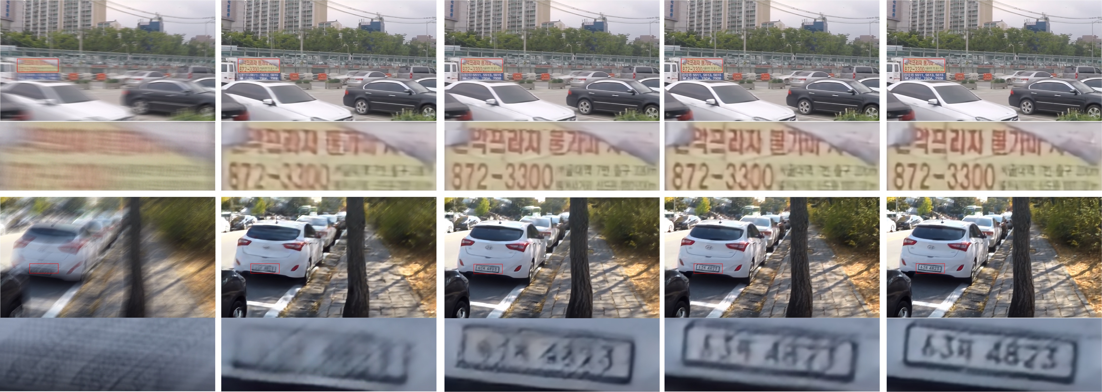
Figure 11: Visual comparison of component analysis on GOPRO dataset. The first column is blurry frame, and 2 $\sim$ 5 columns correspond to the results of 1 $\sim$ 4 rows in Table VIII. Zoom in for better view.

IV-D1 Accuracy of Blur-aware Detector

Table VII lists the accuracy of blur-aware detector on two datasets by using different training loss functions, where we utilize the detector trained on REDS to detect videos from GOPRO for evaluating generalization ability. One can see that detector $\mathcal{F}_{\text{Detector}}$ trained with supervised contrastive loss $\mathcal{L}_{\text{contra}}$ has slightly lower accuracy than that using only $\mathcal{L}_{\text{ce}}$ on GOPRO dataset. However, benefiting from contrastive learning, the features $\bm{z}$ between sharp and blurry frames can be forced as distinguishable as possible, leading to better generalization ability. That is to say the detector trained by cross-entropy loss may be overfitted to training set while failing to handle real-world blurry videos. From the third row in Table VII, the detector trained with supervised contrastive loss performs much better. Moreover, we also detect sharp frames on real-world dataset BSD, where almost 80$\%$ of the detected sharp frames are consistent with human visual observation, further indicating the advantages of $\mathcal{L}_{\text{contra}}$ on generalization ability. In Table V, for the videos without sharp frames as guidance, our method is still superior to the competing methods.

IV-D2 Effectiveness of Hybrid Transformer for Video Deblurring

We evaluate the contribution of each component of proposed video deblurring framework. The experiments are conducted on GOPRO dataset. Self-attention means taking only current frame as input of $f_{\text{cswt}}$, and using self-attention in W-MCA and SW-MCA instead of cross-attention. And the variant with self-attention and global attention takes current blurry frame and its long-term sharp frames as input, while discarding its two neighboring frames From Table VIII and Fig. 11, one can see that long-term sharp features aggregated by global attention bring about 1dB PSNR gain, indicating the effectiveness of global Transformer for aggregating long-term sharp features. By adopting cross-attention, features from neighboring frames can be well exploited, leading to better performance. In our final model, the superior results validated the necessity of adopting cross-attention for aggregating neighboring frames and global attention for aggregating long-term sharp frames for the best deblurring performance.

Besides these key variants of proposed framework in Table VIII, we further discuss another case of cross-attention. Since it is a natural strategy to directly take detected sharp frames and neighboring frames as input of local Transformer, we directly take five frames $\{\bm{G}_{i}^{-},\bm{B}_{i-1},\bm{B}_{i},\bm{B}_{i+1},\bm{G}_{i}^{+}\}$ as input of $f_{\text{cswt}}$ as input while removing global Transformer. In this case, we obtain the results with PSNR 34.19dB and SSIM 0.952, which is much inferior to our final model. The reason can be attributed from two aspects: (i) Neighboring frames and detected sharp frames have different temporal distances, bringing more difficulty for the feature fusion by using one ${f}_{\text{cswt}}$. (ii) Detected sharp frames from a long temporal distance may have dramatic scene changes with the blurry frame, which may be beyond the range of window-based cross-attention.

V Conclusion

In this paper, we proposed a video deblurring framework by aggregating long-term sharp features. First, a blur-aware detector is trained to distinguish between blurry and sharp frames, enabling the identification of long-term sharp frames for facilitating the restoration of a blurry frame. Then, we adopt a hybrid Transformer approach for video deblurring, employing window-based local Transformers to aggregate features from neighboring frames and global Transformers to aggregate long-term sharp features in a multi-scale scheme. Our method can be easily extended to event-driven video deblurring by incorporating an event fusion module. Extensive experimental results on benchmark datasets validate the effectiveness of our approach in terms of both quantitative metrics and visual quality. The learned blur-aware detector and video deblurring network exhibit improved generalization capabilities when handling real-world blurry videos. In future work, our proposed method can be extended to other relevant fields, e.g., video super-resolution, joint video deblurring and multi-frame interpolation.

References

- [1] Z. Zhong, Y. Gao, Y. Zheng, and B. Zheng, “Efficient spatio-temporal recurrent neural network for video deblurring,” in European Conference on Computer Vision, pp. 191–207, 2020.
- [2] H. S. Lee, J. Kwon, and K. M. Lee, “Simultaneous localization, mapping and deblurring,” in IEEE International Conference on Computer Vision, pp. 1203–1210, 2011.
- [3] H. Seok Lee and K. Mu Lee, “Dense 3D reconstruction from severely blurred images using a single moving camera,” in IEEE Conference on Computer Vision and Pattern Recognition, pp. 273–280, 2013.
- [4] Y. Wu, H. Ling, J. Yu, F. Li, X. Mei, and E. Cheng, “Blurred target tracking by blur-driven tracker,” in IEEE International Conference on Computer Vision, 2011.
- [5] J. Pan, H. Bai, and J. Tang, “Cascaded deep video deblurring using temporal sharpness prior,” in IEEE Conference on Computer Vision and Pattern Recognition, pp. 3043–3051, 2020.
- [6] W. Shang, D. Ren, D. Zou, J. S. Ren, P. Luo, and W. Zuo, “Bringing events into video deblurring with non-consecutively blurry frames,” in IEEE International Conference on Computer Vision, pp. 4531–4540, 2021.
- [7] S. Nah, S. Son, and K. M. Lee, “Recurrent neural networks with intra-frame iterations for video deblurring,” in IEEE Conference on Computer Vision and Pattern Recognition, pp. 8102–8111, 2019.
- [8] J. Liang, J. Cao, Y. Fan, K. Zhang, R. Ranjan, Y. Li, R. Timofte, and L. Van Gool, “VRT: A video restoration transformer,” arXiv preprint arXiv:2201.12288, 2022.
- [9] J. Liang, Y. Fan, X. Xiang, R. Ranjan, E. Ilg, S. Green, J. Cao, K. Zhang, R. Timofte, and L. V. Gool, “Recurrent video restoration transformer with guided deformable attention,” Advances in Neural Information Processing Systems, vol. 35, pp. 378–393, 2022.
- [10] X. Yu, F. Xu, S. Zhang, and L. Zhang, “Efficient patch-wise non-uniform deblurring for a single image,” IEEE Transactions on Multimedia, vol. 16, pp. 1510–1524, 2014.
- [11] X. Tao, H. Gao, X. Shen, J. Wang, and J. Jia, “Scale-recurrent network for deep image deblurring,” in IEEE Conference on Computer Vision and Pattern Recognition, pp. 8174–8182, 2018.
- [12] D. Ren, K. Zhang, Q. Wang, Q. Hu, and W. Zuo, “Neural blind deconvolution using deep priors,” in IEEE Conference on Computer Vision and Pattern Recognition, pp. 3341–3350, 2020.
- [13] S.-J. Cho, S.-W. Ji, J.-P. Hong, S.-W. Jung, and S.-J. Ko, “Rethinking coarse-to-fine approach in single image deblurring,” in IEEE International Conference on Computer Vision, pp. 4641–4650, 2021.
- [14] T. Hyun Kim, K. Mu Lee, B. Scholkopf, and M. Hirsch, “Online video deblurring via dynamic temporal blending network,” in IEEE International Conference on Computer Vision, pp. 4038–4047, 2017.
- [15] T. H. Kim, M. S. Sajjadi, M. Hirsch, and B. Scholkopf, “Spatio-temporal transformer network for video restoration,” in European Conference on Computer Vision, pp. 106–122, 2018.
- [16] M. Delbracio and G. Sapiro, “Hand-held video deblurring via efficient fourier aggregation,” IEEE Transactions on Computational Imaging, vol. 1, no. 4, pp. 270–283, 2015.
- [17] J. Pan, B. Xu, H. Bai, J. Tang, and M.-H. Yang, “Cascaded deep video deblurring using temporal sharpness prior and non-local spatial-temporal similarity,” IEEE Transactions on Pattern Analysis and Machine Intelligence, 2023.
- [18] K. Zhang, W. Luo, Y. Zhong, L. Ma, W. Liu, and H. Li, “Adversarial spatio-temporal learning for video deblurring,” IEEE Transactions on Image Processing, vol. 28, no. 1, pp. 291–301, 2018.
- [19] H. Chen, J. Gu, O. Gallo, M.-Y. Liu, A. Veeraraghavan, and J. Kautz, “Reblur2deblur: Deblurring videos via self-supervised learning,” in IEEE International Conference on Computational Photography, pp. 1–9, 2018.
- [20] S. Su, M. Delbracio, J. Wang, G. Sapiro, W. Heidrich, and O. Wang, “Deep video deblurring for hand-held cameras,” in IEEE Conference on Computer Vision and Pattern Recognition, pp. 1279–1288, 2017.
- [21] O. Kupyn, V. Budzan, M. Mykhailych, D. Mishkin, and J. Matas, “DeblurGAN: Blind motion deblurring using conditional adversarial networks,” in IEEE Conference on Computer Vision and Pattern Recognition, pp. 8183–8192, 2018.
- [22] P. Wieschollek, M. Hirsch, B. Scholkopf, and H. Lensch, “Learning blind motion deblurring,” in IEEE International Conference on Computer Vision, pp. 231–240, 2017.
- [23] Y. Zhang, C. Wang, and D. Tao, “Video frame interpolation without temporal priors,” in Advances in Neural Information Processing Systems, pp. 13308–13318, 2020.
- [24] T. Kim, J. Lee, L. Wang, and K.-J. Yoon, “Event-guided deblurring of unknown exposure time videos,” in European Conference on Computer Vision, pp. 519–538, 2022.
- [25] Q. C. Xuanchi Ren, Zian Qian, “Video deblurring by fitting to test data,” in arxiv, 2020.
- [26] S. Nah, T. Hyun Kim, and K. Mu Lee, “Deep multi-scale convolutional neural network for dynamic scene deblurring,” in IEEE Conference on computer vision and pattern recognition, pp. 3883–3891, 2017.
- [27] C. Scheerlinck, H. Rebecq, T. Stoffregen, N. Barnes, R. Mahony, and D. Scaramuzza, “CED: color event camera dataset,” in IEEE Conference on Computer Vision and Pattern Recognition Workshops, pp. 0–0, 2019.
- [28] L. Pan, C. Scheerlinck, X. Yu, R. Hartley, M. Liu, and Y. Dai, “Bringing a blurry frame alive at high frame-rate with an event camera,” in IEEE Conference on Computer Vision and Pattern Recognition, pp. 6820–6829, 2019.
- [29] M. Aittala and F. Durand, “Burst image deblurring using permutation invariant convolutional neural networks,” in European Conference on Computer Vision, pp. 731–747, 2018.
- [30] H. Zhang, Y. Dai, H. Li, and P. Koniusz, “Deep stacked hierarchical multi-patch network for image deblurring,” in IEEE Conference on Computer Vision and Pattern Recognition, pp. 5978–5986, 2019.
- [31] J. Li, B. Yan, Q. Lin, A. Li, and C. Ma, “Motion blur removal with quality assessment guidance,” IEEE Transactions on Multimedia, vol. 23, pp. 2986–2997, 2021.
- [32] X. Wang, K. C. Chan, K. Yu, C. Dong, and C. Change Loy, “EDVR: Video restoration with enhanced deformable convolutional networks,” in IEEE Conference on Computer Vision and Pattern Recognition Workshops, pp. 0–0, 2019.
- [33] L. Patrick, C. Posch, and T. Delbruck, “A 128128 120 db 15s latency asynchronous temporal contrast vision sensor,” IEEE Journal of Solid-state Circuits, vol. 43, pp. 566–576, 2008.
- [34] C. Brandli, R. Berner, M. Yang, S.-C. Liu, and T. Delbruck, “A 240180 130 db 3 s latency global shutter spatiotemporal vision sensor,” IEEE Journal of Solid-State Circuits, vol. 49, no. 10, pp. 2333–2341, 2014.
- [35] A. Mitrokhin, C. Fermüller, C. Parameshwara, and Y. Aloimonos, “Event-based moving object detection and tracking,” in IEEE International Conference on Intelligent Robots and Systems, pp. 1–9, 2018.
- [36] A. Andreopoulos, H. J. Kashyap, T. K. Nayak, A. Amir, and M. D. Flickner, “A low power, high throughput, fully event-based stereo system,” in IEEE Conference on Computer Vision and Pattern Recognition, pp. 7532–7542, 2018.
- [37] M. Liu and T. Delbruck, “Adaptive time-slice block-matching optical flow algorithm for dynamic vision sensors,” British Machine Vision Conference, 2018.
- [38] G. Munda, C. Reinbacher, and T. Pock, “Real-time intensity-image reconstruction for event cameras using manifold regularisation,” International Journal of Computer Vision, vol. 126, no. 12, pp. 1381–1393, 2018.
- [39] H. Rebecq, R. Ranftl, V. Koltun, and D. Scaramuzza, “High speed and high dynamic range video with an event camera,” IEEE Transactions on Pattern Analysis and Machine Intelligence, 2019.
- [40] H. Chen, M. Teng, B. Shi, Y. Wang, and T. Huang, “A residual learning approach to deblur and generate high frame rate video with an event camera,” IEEE Transactions on Multimedia, 2022.
- [41] Z. Jiang, Y. Zhang, D. Zou, J. Ren, J. Lv, and Y. Liu, “Learning event-based motion deblurring,” in IEEE Conference on Computer Vision and Pattern Recognition, pp. 3320–3329, 2020.
- [42] B. Wang, J. He, L. Yu, G.-S. Xia, and W. Yang, “Event enhanced high-quality image recovery,” in European Conference on Computer Vision, pp. 155–171, 2020.
- [43] A. Dosovitskiy, L. Beyer, A. Kolesnikov, D. Weissenborn, X. Zhai, T. Unterthiner, M. Dehghani, M. Minderer, G. Heigold, S. Gelly, et al., “An image is worth 1616 words: Transformers for image recognition at scale,” in International Conference on Learning Representations, 2021.
- [44] N. Carion, F. Massa, G. Synnaeve, N. Usunier, A. Kirillov, and S. Zagoruyko, “End-to-end object detection with transformers,” in European Conference on Computer Vision, pp. 213–229, 2020.
- [45] H. Chen, Y. Wang, T. Guo, C. Xu, Y. Deng, Z. Liu, S. Ma, C. Xu, C. Xu, and W. Gao, “Pre-trained image processing transformer,” in IEEE Conference on Computer Vision and Pattern Recognition, pp. 12299–12310, 2021.
- [46] J. Liang, J. Cao, G. Sun, K. Zhang, L. Van Gool, and R. Timofte, “SwinIR: Image restoration using swin transformer,” in IEEE International Conference on Computer Vision Workshops, pp. 1833–1844, IEEE Computer Society, 2021.
- [47] S. W. Zamir, A. Arora, S. Khan, M. Hayat, F. S. Khan, and M.-H. Yang, “Restormer: Efficient transformer for high-resolution image restoration,” in IEEE conference on computer vision and pattern recognition, pp. 5728–5739, 2022.
- [48] Z. Wang, X. Cun, J. Bao, W. Zhou, J. Liu, and H. Li, “Uformer: A general u-shaped transformer for image restoration,” in IEEE conference on computer vision and pattern recognition, pp. 17683–17693, 2022.
- [49] Z. Liu, Y. Lin, Y. Cao, H. Hu, Y. Wei, Z. Zhang, S. Lin, and B. Guo, “Swin transformer: Hierarchical vision transformer using shifted windows,” IEEE International Conference on Computer Vision), 2021.
- [50] F. Yang, H. Yang, J. Fu, H. Lu, and B. Guo, “Learning texture transformer network for image super-resolution,” in IEEE Conference on Computer Vision and Pattern Recognition, June 2020.
- [51] S. Hochreiter and M. C. Mozer, “A discrete probabilistic memory model for discovering dependencies in time,” in International Conference on Artificial Neural Networks, pp. 661–668, 2001.
- [52] S. Zhou, J. Zhang, J. Pan, H. Xie, W. Zuo, and J. Ren, “Spatio-temporal filter adaptive network for video deblurring,” in IEEE International Conference on Computer Vision, pp. 2482–2491, 2019.
- [53] L. Yu, B. Wang, X. Zhang, H. Zhang, W. Yang, J. Liu, and G.-S. Xia, “Learning to super-resolve blurry images with events,” IEEE Transactions on Pattern Analysis and Machine Intelligence, 2023.
- [54] T. Kalluri, D. Pathak, M. Chandraker, and D. Tran, “FLAVR: Flow-agnostic video representations for fast frame interpolation,” in IEEE Conference on Computer Vision and Pattern Recognition, 2021.
- [55] H. Jiang and Y. Zheng, “Learning to see moving objects in the dark,” in IEEE International Conference on Computer Vision, pp. 7324–7333, 2019.
- [56] D. P. Kingma and J. Ba, “Adam: A method for stochastic optimization,” International Conference on Learning Representations, 2015.