Pearl’s and Jeffrey’s Update as
Modes of Learning in Probabilistic Programming

Abstract

The concept of updating a probability distribution in the light of new evidence lies at the heart of statistics and machine learning. Pearl’s and Jeffrey’s rule are two natural update mechanisms which lead to different outcomes, yet the similarities and differences remain mysterious. This paper clarifies their relationship in several ways: via separate descriptions of the two update mechanisms in terms of probabilistic programs and sampling semantics, and via different notions of likelihood (for Pearl and for Jeffrey). Moreover, it is shown that Jeffrey’s update rule arises via variational inference. In terms of categorical probability theory, this amounts to an analysis of the situation in terms of the behaviour of the multiset functor, extended to the Kleisli category of the distribution monad.

1 Introduction

Suppose you test for a certain disease, say Covid. You take three consecutive tests, because you wish to be sure – two of them come out positive but one is negative. How do you compute the subsequent (posterior) probability that you actually have the disease? In a medical setting one starts from a prevalence, that is, an a priori disease probability, which is assumed to hold for the whole population. Medical tests are typically not perfect: one has to take their sensitivity and specificity into a account. They tell, respectively, if someone has the disease, the probability that the test is positive, and if someone does not have the disease, the probability that the test is negative.

When all these probabilities (prevalence, sensitivity, specificity) are known, one can apply Bayes’ rule and obtain the posterior probability after a single test. But what if we do three tests? And what if we do a thousand tests?

It turns out that things become fuzzy when tests are repeated multiple times. One can distinguish two approaches, associated with Pearl and Jeffrey. They agree on single tests. But they may disagree wildly on multiple tests, see the example in Section 2 below. This is disconcerting, certainly in the current age of machine learning, in which so many decisions are based on statistical learning and decision making.

Earlier work (of one of the authors) [6, 8] analysed the approaches of Pearl and Jeffrey. The difference there was formulated in terms of learning from ‘what is right’ and from ‘what is wrong’. As will be recalled below, Pearl’s update rule involves increasing validity (expected value), whereas Jeffrey’s rule involves decreasing (Kullback-Leibler) divergence. The contributions of this paper are threefold.

• It adds the perspective of probabilistic programming. Pearl’s and Jeffrey’s approaches to updating are formulated, for the medical test example, in a standard probabilistic programming language, namely WebPPL [4, 5], see Section 2. Pearl’s update is straightforwardly expressible using built-in conditioning constructs, while Jeffrey’s update involves nested inference, a simple form of reasoning about reasoning [13]. We further explore the different dynamics behind the two update techniques are operationally using rejection samplers in Section 6.

• The paper also offers a new perspective on the Pearl/Jeffrey distinction in terms of different underlying generative models and their associated likelihoods: with Pearl’s update rule one increases one form of ‘Pearl’ likelihood, whereas with Jeffrey’s update rule one increases another form of ‘Jeffrey’ likelihood. These two likelihoods are described in terms of different forms of evaluating data (as a multiset of data points) with respect to a multinomial distribution. Theses two forms of likelihood are directly related to the respective update mechanisms, see Section 7. Pearl likelihood occurs in practice, for example as the basis of the multinomial naive Bayes classifer [12], while Jeffrey likelihood — and its difference to Pearl’s — is new, as far as we know.

• Pearl’s likelihood directly leads to the associated update rule, see Theorem 7.3. For Jeffrey’s likelihood the connection is more subtle and involves variational inference [10, 11]: it is shown that Jeffrey’s update is least divergent from the update rule for Jeffrey likelihood, in a suitable sense, see Theorem 8.5. This likelihood update rule is described categorically in terms of the extension of the multiset functor to the Kleisli category of the (discrete) distribution monad, see [3, 7]. This analysis clarifies the mathematical situation, for instance in Equation 11, where it is shown that this extended multiset functor commutes with the ‘dagger’ reversal of channels. This is a new result, with a certain esthetic value.

This paper develops the idea that Pearl’s and Jeffrey’s rule involve a difference in perspective: are we trying to learn something about an individual or about a population?

2 A Motivating Example

Consider some disease with an a priori probability (or ‘prevalence’) of $5\%$. There is a test for the disease with the following characteristics:

• (‘sensitivity’) If someone has the disease, then the test is positive with probability of $90\%$.

• (‘specificity’) If someone does not have the disease, there is a $95\%$ chance that the test is negative.

We are told that someone takes three consecutive tests and sees two positive and one negative outcome. These test outcomes are our observed data that we wish to learn from.

The question is: what is the posterior probability that this person has the disease, in the light of this test data? You may wish to stop reading here and calculate this probability yourself. Outcomes, using Pearl’s and Jeffrey’s rule, will be provided in Examples 4.3 and 5.2 below.

Below we present several possible implementations of the medical test situation in the probabilistic programming language WebPPL [4, 5], giving three different solutions to the above question. The code starts by defining a function test which models the test outcome, incorporating the above sensitivity and specificity. Here, flip(p) tosses a biased coin with bias p.

⬇

var test = function(dis) {

return dis ? (flip(0.9) ? ’pos’ : ’neg’) : (flip(0.95) ? ’neg’ : ’pos’);

}

We then define three inference functions which we simply label as prog1, prog2, prog3. At this stage we do not wish to connect them to Pearl/Jeffrey. We invite the reader to form a judgement about what is the ‘right’ way to model the above situation with three test outcomes (‘pos’, ‘pos’, ‘neg’).

⬇

var prog1 = function() {

var dis = flip(0.05);

condition(test(dis) == ’pos’);

condition(test(dis) == ’pos’);

condition(test(dis) == ’neg’);

return dis;

}

var prog2 = function() {

var target = uniformDraw([’pos’,’pos’,’neg’]);

var dis = flip(0.05);

condition(test(dis) == target);

return dis;

}

var prog3 = function() {

var target = uniformDraw([’pos’,’pos’,’neg’]);

return sample(Infer(function() {

var dis = flip(0.05);

condition(test(dis) == target);

return dis;

}))

}

All functions make use of the condition command to instruct WebPPL to compute a conditional probability distribution. prog1 uses three successive conditions, while the other two use a single condition on a randomly chosen target. prog3 additionally makes use of nested inference, that is, it wraps the Infer function around part of its code. Nested inference is a form of reasoning about reasoning [13] and has been applied for example to the study of social cognition, linguistics and theory of mind [5, Ch. 6]. We give a short overview of WebPPL’s semantics and usage in Section 10. All programs can be run using exhaustive enumeration or rejection sampling as inference algorithms, which we elaborate further in Section 4.

The three functions can be executed in WebPPL and the posteriors visualized using the command viz(Infer(prog1)). The posterior disease probabilities of each of the programs are respectively:

• prog1: $64\%$

• prog2: $9\%$

• prog3: $33\%$

The same probabilities appear in the mathematical analysis in Examples 4.3 and 5.2 below.

An interesting question to ask is: suppose we do not have 3 tests (2 positive, 1 negative), but 3000 tests (2000 positive, 1000 negative). Does that change the outcome of the above computations? Not so for the second and third program, which only require a statistical sample of the data. The first program however, quickly converges to $100\%$ disease probability when the number of tests increases (still assuming the same ratio of 2 positive and 1 negative). But this first program becomes increasingly difficult to compute, because each test result emits further conditioning instructions that the inference engine needs to take into account. The two other programs on the other hand scale almost trivially. We return to this scaling issue at the end of Section 7.

The three implementations will be reiterated throughout the paper and related to Pearl’s and Jeffrey’s update. In Section 6, where we also make their semantics explicit using rejection samplers.

3 Multisets, Distributions, and Channels

Sections 3 – 5 introduce the mathematics underlying the update situations that we are looking at. This material is in essence a recap from [6, 8]. We write $\mathcal{M}$ and $\mathcal{D}$ for the multiset and distribution monads on the category $\mathbf{Sets}$ of sets and functions. For a set $X$, multisets $\varphi\in\mathcal{M}(X)$ can equivalently be written as a function $\varphi\colon X\rightarrow\mathbb{N}$ with finite support, or as a finite formal sum $\sum_{i}n_{i}|{\kern 1.00006pt}x_{i}{\kern 1.00006pt}\rangle$, where $n_{i}\in\mathbb{N}$ is the multiplicity of element $x_{i}\in X$. Similarly, a distribution $\omega\in\mathcal{D}(X)$ is written either as a function $\omega\colon X\rightarrow[0,1]$ with finite support and $\sum_{x}\omega(x)=1$, or as a finite formal convex combination $\sum_{i}r_{i}|{\kern 1.00006pt}x_{i}{\kern 1.00006pt}\rangle$ with $r_{i}\in[0,1]$ satisfying $\sum_{i}r_{i}=1$.

Functoriality of $\mathcal{M}$ (and $\mathcal{D}$) works in the following manner. For a function $f\colon X\rightarrow Y$ we have $\mathcal{M}(f)\colon\mathcal{M}(X)\rightarrow\mathcal{M}(Y)$, given as $\mathcal{M}(f)(\varphi)(y)=\sum_{x\in f^{-1}(y)}\varphi(x)$.

For a multiset $\varphi\in\mathcal{M}(X)$ we write $\|\varphi\|\in\mathbb{N}$ for its size, defined as sum of its multiplicities: $\|\varphi\|\coloneqq\sum_{x}\varphi(x)$. When this size is not zero, we can define an associated distribution $\mathsl{flrn}(\varphi)\in\mathcal{D}(X)$, via frequentist learning (normalisation), as:

$$\begin{array}[]{rcl}\mathsl{flrn}(\varphi)&\coloneqq&\displaystyle\sum_{x\in X}\frac{\varphi(x)}{\|\varphi\|}\,\big{|}{\kern 1.00006pt}x{\kern 1.00006pt}\big{\rangle}.\end{array}$$

For $K\in\mathbb{N}$ we write $\mathcal{M}[K](X)=\{\varphi\in\mathcal{M}(X)\;|\;\|\varphi\|=K\}$ for the set of multiset of size $K$. There is an accumulation function $\mathsl{acc}\colon X^{K}\rightarrow\mathcal{M}[K](X)$, given by $\mathsl{acc}(x_{1},\ldots,x_{K})=1|{\kern 1.00006pt}x_{1}{\kern 1.00006pt}\rangle+\cdots+1|{\kern 1.00006pt}x_{K}{\kern 1.00006pt}\rangle$. For instance $\mathsl{acc}(a,b,a,c,a,b)=3|{\kern 1.00006pt}a{\kern 1.00006pt}\rangle+2|{\kern 1.00006pt}b{\kern 1.00006pt}\rangle+1|{\kern 1.00006pt}c{\kern 1.00006pt}\rangle$, using $X=\{a,b,c\}$ and $K=6$.

For two distributions $\omega\in\mathcal{D}(X)$, $\rho\in\mathcal{D}(Y)$ one can form the (parallel) product distribution $\omega\otimes\rho\in\mathcal{D}(X\times Y)$, with $\big{(}\omega\otimes\rho\big{)}(x,y)=\omega(x)\cdot\rho(y)$. We often use the $K$-fold product $\omega^{K}=\omega\otimes\cdots\otimes\omega\in\mathcal{D}(X^{K})$.

A distribution $\omega\in\mathcal{D}(X)$ may be seen as an urn with coloured balls, where $X$ is the set of colours. The number $\omega(x)\in[0,1]$ is the probability of drawing a ball of colour $x$. We are interested in $K$-sized draws, formalised as multiset $\varphi\in\mathcal{M}[K](X)$. The multinomial distribution $\mathsl{mn}[K](\omega)\in\mathcal{D}\big{(}\mathcal{M}[K](X)\big{)}$ assigns probabilities to such draws:

$$\begin{array}[]{rclcrcl}\mathsl{mn}[K](\omega)\hskip 2.0pt\coloneqq\hskip 2.0pt\mathcal{D}(\mathsl{acc})\big{(}\omega^{K}\big{)}&=&\displaystyle\sum_{\varphi\in\mathcal{M}[K](X)}\,\textpdfrender{TextRenderingMode=FillStroke,LineWidth={},}{(}{\kern 1.0pt}\varphi{\kern 1.0pt}\textpdfrender{TextRenderingMode=FillStroke,LineWidth={},}{)}\cdot\prod_{x\in X}\omega(x)^{\varphi(x)}\,\big{|}{\kern 1.00006pt}\varphi{\kern 1.00006pt}\big{\rangle}&\mbox{\quad where \quad}&\textpdfrender{TextRenderingMode=FillStroke,LineWidth={},}{(}{\kern 1.0pt}\varphi{\kern 1.0pt}\textpdfrender{TextRenderingMode=FillStroke,LineWidth={},}{)}&\coloneqq&\displaystyle\frac{\|\varphi\|!}{\prod_{x}\varphi(x)!}.\end{array}$$ (1)

A Kleisli map $c\colon X\rightarrow\mathcal{D}(Y)$ for the distribution monad $\mathcal{D}$ is often called a channel, and written as $c\colon X\mathrel{\ooalign{$\rightarrow$\cr\hfil\!$\leavevmode\hbox{\set@color \leavevmode\hbox to2.6pt{\vbox to2.6pt{\text{[drawing]}}}}$\hfil\cr}}Y$. For instance, the above accumulation map $\mathsl{acc}\colon X^{K}\rightarrow\mathcal{M}[K](X)$ has a probabilistic inverse $\mathsl{arr}\colon\mathcal{M}[K](X)\rightarrow\mathcal{D}(X^{K})$, where $\mathsl{arr}$ stands for arrangement, see [7] for details. This arrangement is defined as:

$$\begin{array}[]{rcl}\mathsl{arr}(\varphi)&\coloneqq&\displaystyle\sum_{\vec{x}\in\mathsl{acc}^{-1}(\varphi)}\,\frac{1}{\textpdfrender{TextRenderingMode=FillStroke,LineWidth={},}{(}{\kern 1.0pt}\varphi{\kern 1.0pt}\textpdfrender{TextRenderingMode=FillStroke,LineWidth={},}{)}}\,\big{|}{\kern 1.00006pt}\vec{x}{\kern 1.00006pt}\big{\rangle}\qquad\mbox{with $\textpdfrender{TextRenderingMode=FillStroke,LineWidth={},}{(}{\kern 1.0pt}\varphi{\kern 1.0pt}\textpdfrender{TextRenderingMode=FillStroke,LineWidth={},}{)}$ as defined in~{}\eqref{MultinomialEqn}.}\end{array}$$ (2)

Kleisli extension gives a pushforward operation along a channel: a distribution $\omega\in\mathcal{D}(X)$ can be turned into a distribution $c\mathrel{\mathchoice{\scalebox{-0.5}[1.0]{$=\ll$}}{\scalebox{-0.5}[1.0]{$={\kern-6.45831pt}\ll$}}{\scalebox{-0.5}[1.0]{${\kern 2.15277pt}\scriptstyle={\kern-0.60275pt}\ll{\kern 1.50694pt}$}}{\scalebox{-0.5}[1.0]{$\scriptscriptstyle=\ll$}}}\omega\in\mathcal{D}(Y)$ via the formula:

$$\begin{array}[]{rcl}c\mathrel{\mathchoice{\scalebox{-0.5}[1.0]{$=\ll$}}{\scalebox{-0.5}[1.0]{$={\kern-6.45831pt}\ll$}}{\scalebox{-0.5}[1.0]{${\kern 2.15277pt}\scriptstyle={\kern-0.60275pt}\ll{\kern 1.50694pt}$}}{\scalebox{-0.5}[1.0]{$\scriptscriptstyle=\ll$}}}\omega&\coloneqq&\displaystyle\sum_{y\in Y}\left(\sum_{x\in X}\omega(x)\cdot c(x)(y)\right)\big{|}{\kern 1.00006pt}y{\kern 1.00006pt}\big{\rangle}.\end{array}$$

This new distribution $c\mathrel{\mathchoice{\scalebox{-0.5}[1.0]{$=\ll$}}{\scalebox{-0.5}[1.0]{$={\kern-6.45831pt}\ll$}}{\scalebox{-0.5}[1.0]{${\kern 2.15277pt}\scriptstyle={\kern-0.60275pt}\ll{\kern 1.50694pt}$}}{\scalebox{-0.5}[1.0]{$\scriptscriptstyle=\ll$}}}\omega$ is often called the prediction. One can prove: $\mathsl{flrn}\mathrel{\mathchoice{\scalebox{-0.5}[1.0]{$=\ll$}}{\scalebox{-0.5}[1.0]{$={\kern-6.45831pt}\ll$}}{\scalebox{-0.5}[1.0]{${\kern 2.15277pt}\scriptstyle={\kern-0.60275pt}\ll{\kern 1.50694pt}$}}{\scalebox{-0.5}[1.0]{$\scriptscriptstyle=\ll$}}}\mathsl{mn}[K](\omega)=\omega$ and $\mathsl{arr}\mathrel{\mathchoice{\scalebox{-0.5}[1.0]{$=\ll$}}{\scalebox{-0.5}[1.0]{$={\kern-6.45831pt}\ll$}}{\scalebox{-0.5}[1.0]{${\kern 2.15277pt}\scriptstyle={\kern-0.60275pt}\ll{\kern 1.50694pt}$}}{\scalebox{-0.5}[1.0]{$\scriptscriptstyle=\ll$}}}\mathsl{mn}[K](\omega)=\omega^{K}$, see [7].

The following two programs are equivalent ways of sampling from a prediction $c\mathrel{\mathchoice{\scalebox{-0.5}[1.0]{$=\ll$}}{\scalebox{-0.5}[1.0]{$={\kern-6.45831pt}\ll$}}{\scalebox{-0.5}[1.0]{${\kern 2.15277pt}\scriptstyle={\kern-0.60275pt}\ll{\kern 1.50694pt}$}}{\scalebox{-0.5}[1.0]{$\scriptscriptstyle=\ll$}}}\omega$:

⬇ x $$\leftarrow\, \omega \leftarrow\, c \leftarrow\, c\mathrel{\mathchoice{\scalebox{-0.5}[1.0]{$=\ll$}}{\scalebox{-0.5}[1.0]{$={\kern-6.45831pt}\ll$}}{\scalebox{-0.5}[1.0]{${\kern 2.15277pt}\scriptstyle={\kern-0.60275pt}\ll{\kern 1.50694pt}$}}{\scalebox{-0.5}[1.0]{$\scriptscriptstyle=\ll$}}}\omega$$ y (x) samples.add(y)                                ⬇ y samples.add(y) (3)

It shows that such sampling can be done in two steps: The notation $x\leftarrow\omega$ is used for sampling a random element $x\in X$ from a distribution $\omega\in\mathcal{D}(X)$, where the randomness takes the probabilities in $\omega$ into account. This is a standard construct in probabilistic programming. If multiple samples $x_{i}\leftarrow\omega$ are taken, and accumulated in a multiset $\varphi\in\mathcal{M}(X)$, then the normalisation $\mathsl{flrn}(\varphi)$ of $\varphi$ approaches the original distribution $\omega$.

Lastly, the tensor product $\otimes$ extends pointwise to channels: $(c\otimes d)(x,y)=c(x)\otimes d(y)$. Then one can prove, for instance, $(c\otimes d)\mathrel{\mathchoice{\scalebox{-0.5}[1.0]{$=\ll$}}{\scalebox{-0.5}[1.0]{$={\kern-6.45831pt}\ll$}}{\scalebox{-0.5}[1.0]{${\kern 2.15277pt}\scriptstyle={\kern-0.60275pt}\ll{\kern 1.50694pt}$}}{\scalebox{-0.5}[1.0]{$\scriptscriptstyle=\ll$}}}(\omega\otimes\rho)=(c\mathrel{\mathchoice{\scalebox{-0.5}[1.0]{$=\ll$}}{\scalebox{-0.5}[1.0]{$={\kern-6.45831pt}\ll$}}{\scalebox{-0.5}[1.0]{${\kern 2.15277pt}\scriptstyle={\kern-0.60275pt}\ll{\kern 1.50694pt}$}}{\scalebox{-0.5}[1.0]{$\scriptscriptstyle=\ll$}}}\omega)\otimes(d\mathrel{\mathchoice{\scalebox{-0.5}[1.0]{$=\ll$}}{\scalebox{-0.5}[1.0]{$={\kern-6.45831pt}\ll$}}{\scalebox{-0.5}[1.0]{${\kern 2.15277pt}\scriptstyle={\kern-0.60275pt}\ll{\kern 1.50694pt}$}}{\scalebox{-0.5}[1.0]{$\scriptscriptstyle=\ll$}}}\rho)$.

4 Validity, Conditioning, and Pearl’s Update Rule

A (fuzzy) predicate on a set $X$ is a function $p\colon X\rightarrow[0,1]$. Each element $x\in X$ gives rise to a point predicate $\mathbf{1}_{x}\colon X\rightarrow[0,1]$, with $\mathbf{1}_{x}(y)=1$ if $x=y$ and $\mathbf{1}_{x}(y)=0$ if $x\neq y$. For two predicates $p_{1},p_{2}\colon X\rightarrow[0,1]$ we can form a conjunction $p_{1}\mathrel{\&}p_{2}\colon X\rightarrow[0,1]$ via pointwise multiplication: $(p_{1}\mathrel{\&}p_{2})(x)=p_{1}(x)\cdot p_{2}(x)$.

The validity (or expected value) of a predicate $p\colon X\rightarrow[0,1]$ in a distribution $\omega\in\mathcal{D}(X)$ is written as $\omega\models p$ and defined as:

$$\begin{array}[]{rcl}\omega\models p&\,\coloneqq\,\displaystyle\sum_{x\in X}\omega(x)\cdot p(x).\end{array}$$

When this validity is non-zero we can define the updated distribution $\omega|_{p}\in\mathcal{D}(X)$ as:

$$\begin{array}[]{rcl}\omega|_{p}&\coloneqq&\displaystyle\sum_{x\in X}\frac{\omega(x)\cdot p(x)}{\omega\models p}\,\big{|}{\kern 1.00006pt}x{\kern 1.00006pt}\big{\rangle}.\end{array}$$ (4)

For a channel $c\colon X\mathrel{\ooalign{$\rightarrow$\cr\hfil\!$\leavevmode\hbox{\set@color \leavevmode\hbox to2.6pt{\vbox to2.6pt{\text{[drawing]}}}}$\hfil\cr}}Y$ and a predicate $q\colon Y\rightarrow[0,1]$ on its codomain, we can define a pullback predicate $c\mathrel{\mathchoice{\scalebox{-0.5}[1.0]{$\gg=$}}{\scalebox{-0.5}[1.0]{$\gg{\kern-6.45831pt}=$}}{\scalebox{-0.5}[1.0]{${\kern 2.15277pt}\scriptstyle\gg{\kern-0.60275pt}={\kern 1.50694pt}$}}{\scalebox{-0.5}[1.0]{$\scriptscriptstyle\gg=$}}}q$ on $X$ via the formula:

$$\begin{array}[]{rcl}\big{(}c\mathrel{\mathchoice{\scalebox{-0.5}[1.0]{$\gg=$}}{\scalebox{-0.5}[1.0]{$\gg{\kern-6.45831pt}=$}}{\scalebox{-0.5}[1.0]{${\kern 2.15277pt}\scriptstyle\gg{\kern-0.60275pt}={\kern 1.50694pt}$}}{\scalebox{-0.5}[1.0]{$\scriptscriptstyle\gg=$}}}q\big{)}(x)&\coloneqq&\displaystyle\sum_{y\in Y}c(x)(y)\cdot q(y).\end{array}$$

The following result contains the basic facts that we need here. Proofs can be found for instance in [6, 8].

Lemma 4.1.

For a channel $c\colon X\mathrel{\ooalign{$\rightarrow$\cr\hfil\!$\leavevmode\hbox{\set@color \leavevmode\hbox to2.6pt{\vbox to2.6pt{\text{[drawing]}}}}$\hfil\cr}}Y$, a distribution $\omega\in\mathcal{D}(X)$, predicates $p,p_{1},p_{2}$ on $X$ and $q$ on $Y$,

1. $c\mathrel{\mathchoice{\scalebox{-0.5}[1.0]{$=\ll$}}{\scalebox{-0.5}[1.0]{$={\kern-6.45831pt}\ll$}}{\scalebox{-0.5}[1.0]{${\kern 2.15277pt}\scriptstyle={\kern-0.60275pt}\ll{\kern 1.50694pt}$}}{\scalebox{-0.5}[1.0]{$\scriptscriptstyle=\ll$}}}\omega\models q\,=\,\omega\models c\mathrel{\mathchoice{\scalebox{-0.5}[1.0]{$\gg=$}}{\scalebox{-0.5}[1.0]{$\gg{\kern-6.45831pt}=$}}{\scalebox{-0.5}[1.0]{${\kern 2.15277pt}\scriptstyle\gg{\kern-0.60275pt}={\kern 1.50694pt}$}}{\scalebox{-0.5}[1.0]{$\scriptscriptstyle\gg=$}}}q$;

2. $\omega|_{p_{1}}|_{p_{2}}=\omega|_{p_{1}\mathrel{\&}p_{2}}$;

3. $\omega|_{p}\models p\,\geq\,\omega\models p$. $\square$

The last result shows that a predicate $p$ is ‘more true’ in an updated distribution $\omega|_{p}$ than in the original $\omega$. The next result from [6, 8] contains both the formulation of Pearl’s update, and the associated validity increase.

Theorem 4.2.

Let $c\colon X\mathrel{\ooalign{$\rightarrow$\cr\hfil\!$\leavevmode\hbox{\set@color \leavevmode\hbox to2.6pt{\vbox to2.6pt{\text{[drawing]}}}}$\hfil\cr}}Y$ be a channel with a prior distribution $\omega\in\mathcal{D}(X)$ on its domain and a predicate $q\colon Y\rightarrow[0,1]$ on its codomain. The posterior distribution $\omega_{P}\in\mathcal{D}(X)$ of $\omega$, via Pearl’ update rule, with the evidence predicate $q$, is defined as:

$$\begin{array}[]{rclcrcl}\omega_{P}&\coloneqq&\omega|_{c\mathrel{\mathchoice{\scalebox{-0.5}[1.0]{$\gg=$}}{\scalebox{-0.5}[1.0]{$\gg{\kern-4.52083pt}=$}}{\scalebox{-0.5}[1.0]{${\kern 1.50694pt}\scriptstyle\gg{\kern-0.42192pt}={\kern 1.05486pt}$}}{\scalebox{-0.5}[1.0]{$\scriptscriptstyle\gg=$}}}q}&\mbox{\qquad and satisfies \qquad}&c\mathrel{\mathchoice{\scalebox{-0.5}[1.0]{$=\ll$}}{\scalebox{-0.5}[1.0]{$={\kern-6.45831pt}\ll$}}{\scalebox{-0.5}[1.0]{${\kern 2.15277pt}\scriptstyle={\kern-0.60275pt}\ll{\kern 1.50694pt}$}}{\scalebox{-0.5}[1.0]{$\scriptscriptstyle=\ll$}}}\omega_{P}\models q&\,\geq&c\mathrel{\mathchoice{\scalebox{-0.5}[1.0]{$=\ll$}}{\scalebox{-0.5}[1.0]{$={\kern-6.45831pt}\ll$}}{\scalebox{-0.5}[1.0]{${\kern 2.15277pt}\scriptstyle={\kern-0.60275pt}\ll{\kern 1.50694pt}$}}{\scalebox{-0.5}[1.0]{$\scriptscriptstyle=\ll$}}}\omega\models q.\end{array}$$

The proof follows from an easy combination of points (1) and (3) of Lemma 4.1. The increase in validity that is achieved via Pearl’s rule means that the validity of predicate $q$ is higher in the predicted distribution obtained from the posterior distribution $\omega_{P}$, than in the prediction obtained from original, prior distribution $\omega$.

The following are two rejection samplers that allow sampling from a posterior distribution: On the left below we show how to obtain an updated distribution $\omega|_{p}$ via sampling, and on the right how to get a Pearl update $\omega|_{c\mathrel{\mathchoice{\scalebox{-0.5}[1.0]{$\gg=$}}{\scalebox{-0.5}[1.0]{$\gg{\kern-4.52083pt}=$}}{\scalebox{-0.5}[1.0]{${\kern 1.50694pt}\scriptstyle\gg{\kern-0.42192pt}={\kern 1.05486pt}$}}{\scalebox{-0.5}[1.0]{$\scriptscriptstyle\gg=$}}}q}$.

⬇ x $$\leftarrow\, \omega \leftarrow\, p \leftarrow\, \omega \leftarrow\, c \leftarrow\, q$$ y flip((x)) if y == 1: samples.add(x)                          ⬇ x y (x) z flip((y)) if z == 1: samples.add(x) (5)

The probabilistic program prog1 at the end of Section 2 computes the Pearl update. How this update works in detail will be described next.

Example 4.3.

We are now in a situation to explain the $64\%$ posterior disease probability claimed in Section 2. It is obtained via repeated Pearl updates. We first translate the information given there into mathematical structure.

We use $X=\{d,d^{\scriptscriptstyle\bot}\}$ for the set with elements $d$ for disease and $d^{\scriptscriptstyle\bot}$ for no-disease. The given prevalence of $5\%$ for the disease corresponds to a prior distribution $\omega\in\mathcal{D}(X)$ given by $\omega=\frac{1}{20}|{\kern 1.00006pt}d{\kern 1.00006pt}\rangle+\frac{19}{20}|{\kern 1.00006pt}d^{\scriptscriptstyle\bot}{\kern 1.00006pt}\rangle$.

The test is formalised as a channel $c\colon X\rightarrow\mathcal{D}(Y)$ where $Y=\{p,n\}$ the set of positive and negative test outcomes. The sensitivity and specificity of the test translate into, respectively:

$$\begin{array}[]{rclcrcl}c(d)&\coloneqq&\frac{9}{10}|{\kern 1.00006pt}p{\kern 1.00006pt}\rangle+\frac{1}{10}|{\kern 1.00006pt}n{\kern 1.00006pt}\rangle&\mbox{\qquad and \qquad}&c(d^{\scriptscriptstyle\bot})&\coloneqq&\frac{1}{20}|{\kern 1.00006pt}p{\kern 1.00006pt}\rangle+\frac{19}{20}|{\kern 1.00006pt}n{\kern 1.00006pt}\rangle.\end{array}$$

There are two obvious point predicates $\mathbf{1}_{p}\colon Y\rightarrow[0,1]$ and $\mathbf{1}_{n}\colon Y\rightarrow[0,1]$ on the set $Y=\{p,n\}$ of test outcomes. We are told that there are two positive and one negative test. This translates in the conjunction $(c\mathrel{\mathchoice{\scalebox{-0.5}[1.0]{$\gg=$}}{\scalebox{-0.5}[1.0]{$\gg{\kern-6.45831pt}=$}}{\scalebox{-0.5}[1.0]{${\kern 2.15277pt}\scriptstyle\gg{\kern-0.60275pt}={\kern 1.50694pt}$}}{\scalebox{-0.5}[1.0]{$\scriptscriptstyle\gg=$}}}\mathbf{1}_{p})\mathrel{\&}(c\mathrel{\mathchoice{\scalebox{-0.5}[1.0]{$\gg=$}}{\scalebox{-0.5}[1.0]{$\gg{\kern-6.45831pt}=$}}{\scalebox{-0.5}[1.0]{${\kern 2.15277pt}\scriptstyle\gg{\kern-0.60275pt}={\kern 1.50694pt}$}}{\scalebox{-0.5}[1.0]{$\scriptscriptstyle\gg=$}}}\mathbf{1}_{p})\mathrel{\&}(c\mathrel{\mathchoice{\scalebox{-0.5}[1.0]{$\gg=$}}{\scalebox{-0.5}[1.0]{$\gg{\kern-6.45831pt}=$}}{\scalebox{-0.5}[1.0]{${\kern 2.15277pt}\scriptstyle\gg{\kern-0.60275pt}={\kern 1.50694pt}$}}{\scalebox{-0.5}[1.0]{$\scriptscriptstyle\gg=$}}}\mathbf{1}_{n})$. Since conjunction is commutative, the order does not matter. Updating with this conjection is equivalent to three successive update, see Lemmma 4.1 (2), and gives the claimed outcome:

$$\begin{array}[]{rcl}\omega_{P}\hskip 2.0pt=\hskip 2.0pt\omega\big{|}_{(c\mathrel{\mathchoice{\scalebox{-0.5}[1.0]{$\gg=$}}{\scalebox{-0.5}[1.0]{$\gg{\kern-4.52083pt}=$}}{\scalebox{-0.5}[1.0]{${\kern 1.50694pt}\scriptstyle\gg{\kern-0.42192pt}={\kern 1.05486pt}$}}{\scalebox{-0.5}[1.0]{$\scriptscriptstyle\gg=$}}}\mathbf{1}_{p})\mathrel{\&}(c\mathrel{\mathchoice{\scalebox{-0.5}[1.0]{$\gg=$}}{\scalebox{-0.5}[1.0]{$\gg{\kern-4.52083pt}=$}}{\scalebox{-0.5}[1.0]{${\kern 1.50694pt}\scriptstyle\gg{\kern-0.42192pt}={\kern 1.05486pt}$}}{\scalebox{-0.5}[1.0]{$\scriptscriptstyle\gg=$}}}\mathbf{1}_{p})\mathrel{\&}(c\mathrel{\mathchoice{\scalebox{-0.5}[1.0]{$\gg=$}}{\scalebox{-0.5}[1.0]{$\gg{\kern-4.52083pt}=$}}{\scalebox{-0.5}[1.0]{${\kern 1.50694pt}\scriptstyle\gg{\kern-0.42192pt}={\kern 1.05486pt}$}}{\scalebox{-0.5}[1.0]{$\scriptscriptstyle\gg=$}}}\mathbf{1}_{n})}\hskip 2.0pt=\hskip 2.0pt\omega\big{|}_{c\mathrel{\mathchoice{\scalebox{-0.5}[1.0]{$\gg=$}}{\scalebox{-0.5}[1.0]{$\gg{\kern-4.52083pt}=$}}{\scalebox{-0.5}[1.0]{${\kern 1.50694pt}\scriptstyle\gg{\kern-0.42192pt}={\kern 1.05486pt}$}}{\scalebox{-0.5}[1.0]{$\scriptscriptstyle\gg=$}}}\mathbf{1}_{p}}\big{|}_{c\mathrel{\mathchoice{\scalebox{-0.5}[1.0]{$\gg=$}}{\scalebox{-0.5}[1.0]{$\gg{\kern-4.52083pt}=$}}{\scalebox{-0.5}[1.0]{${\kern 1.50694pt}\scriptstyle\gg{\kern-0.42192pt}={\kern 1.05486pt}$}}{\scalebox{-0.5}[1.0]{$\scriptscriptstyle\gg=$}}}\mathbf{1}_{p}}\big{|}_{c\mathrel{\mathchoice{\scalebox{-0.5}[1.0]{$\gg=$}}{\scalebox{-0.5}[1.0]{$\gg{\kern-4.52083pt}=$}}{\scalebox{-0.5}[1.0]{${\kern 1.50694pt}\scriptstyle\gg{\kern-0.42192pt}={\kern 1.05486pt}$}}{\scalebox{-0.5}[1.0]{$\scriptscriptstyle\gg=$}}}\mathbf{1}_{n}}&=&\frac{648}{1009}\big{|}{\kern 1.00006pt}d{\kern 1.00006pt}\big{\rangle}+\frac{361}{1009}\big{|}{\kern 1.00006pt}d^{\scriptscriptstyle\bot}{\kern 1.00006pt}\big{\rangle}\\ &\approx&0.642\big{|}{\kern 1.00006pt}d{\kern 1.00006pt}\big{\rangle}+0.358\big{|}{\kern 1.00006pt}d^{\scriptscriptstyle\bot}{\kern 1.00006pt}\big{\rangle}.\end{array}$$

This is the probability computed in prog1 in Section 2.

The validity increase associated with Pearl’s update rule takes the following form.

$$\begin{array}[]{rcccccl}c\mathrel{\mathchoice{\scalebox{-0.5}[1.0]{$=\ll$}}{\scalebox{-0.5}[1.0]{$={\kern-6.45831pt}\ll$}}{\scalebox{-0.5}[1.0]{${\kern 2.15277pt}\scriptstyle={\kern-0.60275pt}\ll{\kern 1.50694pt}$}}{\scalebox{-0.5}[1.0]{$\scriptscriptstyle=\ll$}}}\omega_{P}\models(c\mathrel{\mathchoice{\scalebox{-0.5}[1.0]{$\gg=$}}{\scalebox{-0.5}[1.0]{$\gg{\kern-6.45831pt}=$}}{\scalebox{-0.5}[1.0]{${\kern 2.15277pt}\scriptstyle\gg{\kern-0.60275pt}={\kern 1.50694pt}$}}{\scalebox{-0.5}[1.0]{$\scriptscriptstyle\gg=$}}}\mathbf{1}_{p})^{2}\mathrel{\&}(c\mathrel{\mathchoice{\scalebox{-0.5}[1.0]{$\gg=$}}{\scalebox{-0.5}[1.0]{$\gg{\kern-6.45831pt}=$}}{\scalebox{-0.5}[1.0]{${\kern 2.15277pt}\scriptstyle\gg{\kern-0.60275pt}={\kern 1.50694pt}$}}{\scalebox{-0.5}[1.0]{$\scriptscriptstyle\gg=$}}}\mathbf{1}_{n})&\approx&0.049&\,\geq&0.0096&\approx&c\mathrel{\mathchoice{\scalebox{-0.5}[1.0]{$=\ll$}}{\scalebox{-0.5}[1.0]{$={\kern-6.45831pt}\ll$}}{\scalebox{-0.5}[1.0]{${\kern 2.15277pt}\scriptstyle={\kern-0.60275pt}\ll{\kern 1.50694pt}$}}{\scalebox{-0.5}[1.0]{$\scriptscriptstyle=\ll$}}}\omega\models(c\mathrel{\mathchoice{\scalebox{-0.5}[1.0]{$\gg=$}}{\scalebox{-0.5}[1.0]{$\gg{\kern-6.45831pt}=$}}{\scalebox{-0.5}[1.0]{${\kern 2.15277pt}\scriptstyle\gg{\kern-0.60275pt}={\kern 1.50694pt}$}}{\scalebox{-0.5}[1.0]{$\scriptscriptstyle\gg=$}}}\mathbf{1}_{p})^{2}\mathrel{\&}(c\mathrel{\mathchoice{\scalebox{-0.5}[1.0]{$\gg=$}}{\scalebox{-0.5}[1.0]{$\gg{\kern-6.45831pt}=$}}{\scalebox{-0.5}[1.0]{${\kern 2.15277pt}\scriptstyle\gg{\kern-0.60275pt}={\kern 1.50694pt}$}}{\scalebox{-0.5}[1.0]{$\scriptscriptstyle\gg=$}}}\mathbf{1}_{n}).\end{array}$$

5 Dagger channels and Jeffrey’s update rule

First we recall that the difference (divergence) between two distributions $\omega,\rho\in\mathcal{D}(X)$ is commonly expressed as Kullback-Leibler divergence, defined as:

$$\begin{array}[]{rcl}\mathsl{D}_{\mathsl{KL}}\big{(}\omega,\,\rho\big{)}&\coloneqq&\displaystyle\sum_{x\in X}\omega(x)\cdot\ln\left(\frac{\omega(x)}{\rho(x)}\right),\mbox{\qquad where $\ln$ is the natural logarithm.}\end{array}$$ (6)

The main ingredient that we need for Jeffrey’s rule is the dagger of a channel $c\colon X\mathrel{\ooalign{$\rightarrow$\cr\hfil\!$\leavevmode\hbox{\set@color \leavevmode\hbox to2.6pt{\vbox to2.6pt{\text{[drawing]}}}}$\hfil\cr}}Y$ with respect to a prior distribution $\omega\in\mathcal{D}(X)$. This dagger is a channel $c^{{\dagger}}_{\omega}\colon Y\mathrel{\ooalign{$\rightarrow$\cr\hfil\!$\leavevmode\hbox{\set@color \leavevmode\hbox to2.6pt{\vbox to2.6pt{\text{[drawing]}}}}$\hfil\cr}}X$ in the opposite direction. It is also called Bayesian inversion, see [2, 1], and it is defined on $y\in Y$ as:

$$\begin{array}[]{rcccl}c^{{\dagger}}_{\omega}(y)&\coloneqq&\omega|_{c\mathrel{\mathchoice{\scalebox{-0.5}[1.0]{$\gg=$}}{\scalebox{-0.5}[1.0]{$\gg{\kern-4.52083pt}=$}}{\scalebox{-0.5}[1.0]{${\kern 1.50694pt}\scriptstyle\gg{\kern-0.42192pt}={\kern 1.05486pt}$}}{\scalebox{-0.5}[1.0]{$\scriptscriptstyle\gg=$}}}\mathbf{1}_{y}}&\smash{\stackrel{{\scriptstyle\eqref{ConditionEqn}}}{{=}}}&\displaystyle\sum_{x\in X}\,\frac{\omega(x)\cdot c(x)(y)}{(c\mathrel{\mathchoice{\scalebox{-0.5}[1.0]{$=\ll$}}{\scalebox{-0.5}[1.0]{$={\kern-6.45831pt}\ll$}}{\scalebox{-0.5}[1.0]{${\kern 2.15277pt}\scriptstyle={\kern-0.60275pt}\ll{\kern 1.50694pt}$}}{\scalebox{-0.5}[1.0]{$\scriptscriptstyle=\ll$}}}\omega)(y)}\,\big{|}{\kern 1.00006pt}x{\kern 1.00006pt}\big{\rangle}.\end{array}$$ (7)

We again combine Jeffrey’s rule with its main divergence reduction property, from [8]. The set-up is very much as for Pearl’s rule, in Theorem 4.2, but with evidence now in the form of distribution instead of a predicate.

Theorem 5.1.

Let $c\colon X\mathrel{\ooalign{$\rightarrow$\cr\hfil\!$\leavevmode\hbox{\set@color \leavevmode\hbox to2.6pt{\vbox to2.6pt{\text{[drawing]}}}}$\hfil\cr}}Y$ be a channel with a prior distribution $\omega\in\mathcal{D}(X)$ and an evidence distribution $\tau\in\mathcal{D}(Y)$. The posterior distribution $\omega_{J}\in\mathcal{D}(X)$ of $\omega$, obtained via Jeffrey’s update rule, with the evidence distribution $\tau$, is defined as:

$$\begin{array}[]{rclcrcl}\omega_{J}&\coloneqq&c^{{\dagger}}_{\omega}\mathrel{\mathchoice{\scalebox{-0.5}[1.0]{$=\ll$}}{\scalebox{-0.5}[1.0]{$={\kern-6.45831pt}\ll$}}{\scalebox{-0.5}[1.0]{${\kern 2.15277pt}\scriptstyle={\kern-0.60275pt}\ll{\kern 1.50694pt}$}}{\scalebox{-0.5}[1.0]{$\scriptscriptstyle=\ll$}}}\tau&\mbox{\qquad and satisfies \qquad}&\mathsl{D}_{\mathsl{KL}}\big{(}\tau,\,c\mathrel{\mathchoice{\scalebox{-0.5}[1.0]{$=\ll$}}{\scalebox{-0.5}[1.0]{$={\kern-6.45831pt}\ll$}}{\scalebox{-0.5}[1.0]{${\kern 2.15277pt}\scriptstyle={\kern-0.60275pt}\ll{\kern 1.50694pt}$}}{\scalebox{-0.5}[1.0]{$\scriptscriptstyle=\ll$}}}\omega_{J}\big{)}&\,\leq&\mathsl{D}_{\mathsl{KL}}\big{(}\tau,\,c\mathrel{\mathchoice{\scalebox{-0.5}[1.0]{$=\ll$}}{\scalebox{-0.5}[1.0]{$={\kern-6.45831pt}\ll$}}{\scalebox{-0.5}[1.0]{${\kern 2.15277pt}\scriptstyle={\kern-0.60275pt}\ll{\kern 1.50694pt}$}}{\scalebox{-0.5}[1.0]{$\scriptscriptstyle=\ll$}}}\omega\big{)}.\end{array}$$

The proof of this divergence decrease is remarkably hard, see [8] for details. The result says that the prediction from $\omega_{J}$ is less wrong than from $\omega$, when compared to the ‘target’ distribution $\tau$.

Example 5.2.

We build on the test channel $c\colon X\mathrel{\ooalign{$\rightarrow$\cr\hfil\!$\leavevmode\hbox{\set@color \leavevmode\hbox to2.6pt{\vbox to2.6pt{\text{[drawing]}}}}$\hfil\cr}}Y$ and prevalence distribution $\omega\in\mathcal{D}(X)$ from Example 4.3. The first task is to compute the dagger channel $f\coloneqq c^{{\dagger}}_{\omega}\colon Y\mathrel{\ooalign{$\rightarrow$\cr\hfil\!$\leavevmode\hbox{\set@color \leavevmode\hbox to2.6pt{\vbox to2.6pt{\text{[drawing]}}}}$\hfil\cr}}X$. It yields:

$$\begin{array}[]{rclcrcl}f(p)&=&\frac{18}{37}\big{|}{\kern 1.00006pt}d{\kern 1.00006pt}\big{\rangle}+\frac{19}{37}\big{|}{\kern 1.00006pt}d^{\scriptscriptstyle\bot}{\kern 1.00006pt}\big{\rangle}&\mbox{\qquad and \qquad}&f(n)&=&\frac{2}{363}\big{|}{\kern 1.00006pt}d{\kern 1.00006pt}\big{\rangle}+\frac{361}{363}\big{|}{\kern 1.00006pt}d^{\scriptscriptstyle\bot}{\kern 1.00006pt}\big{\rangle}.\end{array}$$

The fact that there are two positive and one negative test translates into the ‘empirical’ evidence distribution $\tau=\frac{2}{3}|{\kern 1.00006pt}p{\kern 1.00006pt}\rangle+\frac{1}{3}|{\kern 1.00006pt}n{\kern 1.00006pt}\rangle\in\mathcal{D}(Y)$. The posterior, updated disease distribution, obtained from this evidence, gives the $33\%$ probability mentioned in Section 2:

$$\begin{array}[]{rcccccl}\omega_{J}&=&f\mathrel{\mathchoice{\scalebox{-0.5}[1.0]{$=\ll$}}{\scalebox{-0.5}[1.0]{$={\kern-6.45831pt}\ll$}}{\scalebox{-0.5}[1.0]{${\kern 2.15277pt}\scriptstyle={\kern-0.60275pt}\ll{\kern 1.50694pt}$}}{\scalebox{-0.5}[1.0]{$\scriptscriptstyle=\ll$}}}\tau&=&\frac{13142}{40293}\big{|}{\kern 1.00006pt}d{\kern 1.00006pt}\big{\rangle}+\frac{27151}{40293}\big{|}{\kern 1.00006pt}d^{\scriptscriptstyle\bot}{\kern 1.00006pt}\big{\rangle}&\approx&0.326\big{|}{\kern 1.00006pt}d{\kern 1.00006pt}\big{\rangle}+0.674\big{|}{\kern 1.00006pt}d^{\scriptscriptstyle\bot}{\kern 1.00006pt}\big{\rangle}.\end{array}$$

This probability is computed by prog3 in Section 2.

The divergence decrease from Theorem 5.1 takes the following form:

$$\begin{array}[]{rcccccl}\mathsl{D}_{\mathsl{KL}}\big{(}\tau,\,c\mathrel{\mathchoice{\scalebox{-0.5}[1.0]{$=\ll$}}{\scalebox{-0.5}[1.0]{$={\kern-6.45831pt}\ll$}}{\scalebox{-0.5}[1.0]{${\kern 2.15277pt}\scriptstyle={\kern-0.60275pt}\ll{\kern 1.50694pt}$}}{\scalebox{-0.5}[1.0]{$\scriptscriptstyle=\ll$}}}\omega_{J}\big{)}&\approx&0.24&\,\leq&0.98&\approx&\mathsl{D}_{\mathsl{KL}}\big{(}\tau,\,c\mathrel{\mathchoice{\scalebox{-0.5}[1.0]{$=\ll$}}{\scalebox{-0.5}[1.0]{$={\kern-6.45831pt}\ll$}}{\scalebox{-0.5}[1.0]{${\kern 2.15277pt}\scriptstyle={\kern-0.60275pt}\ll{\kern 1.50694pt}$}}{\scalebox{-0.5}[1.0]{$\scriptscriptstyle=\ll$}}}\omega\big{)}.\end{array}$$

Having seen this, we may ask: why not use the evidence distribution $\tau=\frac{2}{3}|{\kern 1.00006pt}p{\kern 1.00006pt}\rangle+\frac{1}{3}|{\kern 1.00006pt}n{\kern 1.00006pt}\rangle$ not as a predicate $q=\frac{2}{3}\mathbf{1}_{p}+\frac{1}{3}\mathbf{1}_{n}$, and then do a single Pearl update:

$$\begin{array}[]{rcccl}\omega|_{c\mathrel{\mathchoice{\scalebox{-0.5}[1.0]{$\gg=$}}{\scalebox{-0.5}[1.0]{$\gg{\kern-4.52083pt}=$}}{\scalebox{-0.5}[1.0]{${\kern 1.50694pt}\scriptstyle\gg{\kern-0.42192pt}={\kern 1.05486pt}$}}{\scalebox{-0.5}[1.0]{$\scriptscriptstyle\gg=$}}}q}&=&\frac{2}{23}|{\kern 1.00006pt}d{\kern 1.00006pt}\rangle+\frac{21}{23}|{\kern 1.00006pt}d^{\scriptscriptstyle\bot}{\kern 1.00006pt}\rangle&\approx&0.087|{\kern 1.00006pt}d{\kern 1.00006pt}\rangle+0.913|{\kern 1.00006pt}d^{\scriptscriptstyle\bot}{\kern 1.00006pt}\rangle.\end{array}$$ (8)

This is the distribution computed by program prog2 in Section 2.

For future use we record the following standard properties of the dagger of a channel (7).

Lemma 5.3.

1. Daggers preserve sequential composition: for two successive channels $X\stackrel{{\scriptstyle c}}{{\mathrel{\ooalign{$\rightarrow$\cr\hfil\!$\leavevmode\hbox{\set@color \leavevmode\hbox to2.6pt{\vbox to2.6pt{\text{[drawing]}}}}$\hfil\cr}}}}Y\stackrel{{\scriptstyle d}}{{\mathrel{\ooalign{$\rightarrow$\cr\hfil\!$\leavevmode\hbox{\set@color \leavevmode\hbox to2.6pt{\vbox to2.6pt{\text{[drawing]}}}}$\hfil\cr}}}}Z$ and a distribution $\omega\in\mathcal{D}(X)$,

   $$\begin{array}[]{rcl}\big{(}d\mathbin{\mathchoice{\ooalign{$\displaystyle\circ$\crcr$\displaystyle\cdot$}}{\ooalign{$\textstyle\circ$\crcr$\textstyle\cdot$}}{\ooalign{$\scriptstyle\circ$\crcr$\scriptstyle\cdot$}}{\ooalign{$\scriptscriptstyle\circ$\crcr$\scriptscriptstyle\cdot$}}}c\big{)}_{\omega}^{{\dagger}}&=&c_{\omega}^{{\dagger}}\mathbin{\mathchoice{\ooalign{$\displaystyle\circ$\crcr$\displaystyle\cdot$}}{\ooalign{$\textstyle\circ$\crcr$\textstyle\cdot$}}{\ooalign{$\scriptstyle\circ$\crcr$\scriptstyle\cdot$}}{\ooalign{$\scriptscriptstyle\circ$\crcr$\scriptscriptstyle\cdot$}}}d_{c\mathrel{\mathchoice{\scalebox{-0.5}[1.0]{$=\ll$}}{\scalebox{-0.5}[1.0]{$={\kern-4.52083pt}\ll$}}{\scalebox{-0.5}[1.0]{${\kern 1.50694pt}\scriptstyle={\kern-0.42192pt}\ll{\kern 1.05486pt}$}}{\scalebox{-0.5}[1.0]{$\scriptscriptstyle=\ll$}}}\omega}^{{\dagger}}.\end{array}$$

2. Daggers preserve parallel composition: for two channels $c\colon X\mathrel{\ooalign{$\rightarrow$\cr\hfil\!$\leavevmode\hbox{\set@color \leavevmode\hbox to2.6pt{\vbox to2.6pt{\text{[drawing]}}}}$\hfil\cr}}A$, $d\colon Y\mathrel{\ooalign{$\rightarrow$\cr\hfil\!$\leavevmode\hbox{\set@color \leavevmode\hbox to2.6pt{\vbox to2.6pt{\text{[drawing]}}}}$\hfil\cr}}B$ with distributions $\omega\in\mathcal{D}(X)$, $\rho\in\mathcal{D}(Y$),

   $$\begin{array}[]{rcl}\big{(}c\otimes d\big{)}_{\omega\otimes\rho}^{{\dagger}}&=&c_{\omega}^{{\dagger}}\otimes d_{\rho}^{{\dagger}}.\end{array}$$

6 An Operational Understanding of Jeffrey’s Update

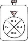
Figure 1: Ticker device

We return to the probabilistic programs of Section 2. As discussed in Section 4, prog1 expresses repeated Pearl updates. It remains to understand the difference between prog2 and prog3. As shown in (8), prog2 corresponds to a single Pearl’s update with the target distribution, as predicate. Further, prog3 is Jeffrey’s update, with the nested inference corresponding to the computation of the dagger channel $c^{\dagger}_{\omega}$. The difference between the two programs prog2 and prog3 is surprisingly subtle, so we begin by illustrating it using a different kind of metaphor, and derive a rejection sampler for each case in turn.

Consider a large queue of people waiting in front of a club. Each person prefers either rock or pop. The club’s management wants to achieve a target ratio of 75% rock fans on the inside. To that end, they equip their doorman with a special ticker device, see Figure 1. The ticker displays a current target (either ‘Rock’ or ‘Pop’), and the doorman admits the next person if and only if they prefer the targeted style. The doorman can click the device to obtain a new target (either by cycling sequentially through the targets, or picking one randomly), but there remains a choice when to click.

1. Single Pearl Policy: pick a new target after every person:

   ⬇

   for person in queue:

   if person.preference == ticker.target:

   club.admit(person)

   ticker.click()

2. Jeffrey Policy: pick a new target only after admitting a person:

   ⬇

   for person in queue:

   if person.preference == ticker.target:

   club.admit(person)

   ticker.click()

It may be clear that only the Jeffrey Policy is suitable to achieve the management’s goal. Approximately 75% of the people which are admitted are rock fans. This is in line with the key property of Jeffrey’s update rule: reducing the divergence with the target distribution $\tau$, see Theorem 5.1. It is unclear what the single Pearl policy achieves in this context.

We may also wonder how the door policy influences other statistical properties of the audience (such as age or gender) which may correlate with music preference: If the prior distribution in the queue is $\omega$, what will the resulting distribution be inside the club? For the Jeffrey Policy, this update is precisely described by Jeffrey’s update. We summarize this section with a concrete description of rejection samplers for Pearl’s update with a random target (left) and Jeffrey’s update (right), corresponding to the semantics of the probabilistic programs prog2 and prog3:

⬇ while True: x $$\leftarrow\, \omega \leftarrow\, \leftarrow\, \tau \leftarrow\, \omega \leftarrow\, \leftarrow\, \tau$$ y c(x) target if y == target: samples.add(x)                 ⬇ while True: x y c(x) if y == target: samples.add(x) target (9)

7 Likelihoods and Generative Models for Pearl and Jeffrey

This section first identifies two forms of likelihood of data in the situation with a statistical model given by a channel $X\mathrel{\ooalign{$\rightarrow$\cr\hfil\!$\leavevmode\hbox{\set@color \leavevmode\hbox to2.6pt{\vbox to2.6pt{\text{[drawing]}}}}$\hfil\cr}}Y$ and a distribution on $X$. It then relates these two forms of likelihood to the two update rules of repeated-Pearl and Jeffrey — in Theorems 4.2 and 5.1.

Definition 7.1.

Let $\psi\in\mathcal{M}[K](Y)$ be a multiset of data, of size $K=\|\psi\|\in\mathbb{N}$. Let $c\colon X\mathrel{\ooalign{$\rightarrow$\cr\hfil\!$\leavevmode\hbox{\set@color \leavevmode\hbox to2.6pt{\vbox to2.6pt{\text{[drawing]}}}}$\hfil\cr}}Y$ be a channel with a distribution $\omega\in\mathcal{D}(X)$ on its domain.

1. The Jeffrey likelihood of the multiset $\psi$ is given by the number:

   $$\mathsl{mn}[K]\big{(}c\mathrel{\mathchoice{\scalebox{-0.5}[1.0]{$=\ll$}}{\scalebox{-0.5}[1.0]{$={\kern-6.45831pt}\ll$}}{\scalebox{-0.5}[1.0]{${\kern 2.15277pt}\scriptstyle={\kern-0.60275pt}\ll{\kern 1.50694pt}$}}{\scalebox{-0.5}[1.0]{$\scriptscriptstyle=\ll$}}}\omega\big{)}(\psi).$$

2. The Pearl likelihood of $\psi$ in the same model is the first expression below, which has several alternative formulations. It uses the abbreviation $\mathsl{mn}[K](c)\coloneqq\mathsl{mn}[K]\mathrel{\circ}c$.

   $$\begin{array}[]{rcl}\big{(}\mathsl{mn}[K](c)\mathrel{\mathchoice{\scalebox{-0.5}[1.0]{$=\ll$}}{\scalebox{-0.5}[1.0]{$={\kern-6.45831pt}\ll$}}{\scalebox{-0.5}[1.0]{${\kern 2.15277pt}\scriptstyle={\kern-0.60275pt}\ll{\kern 1.50694pt}$}}{\scalebox{-0.5}[1.0]{$\scriptscriptstyle=\ll$}}}\omega\big{)}(\psi)&=&\mathsl{mn}[K](c)\mathrel{\mathchoice{\scalebox{-0.5}[1.0]{$=\ll$}}{\scalebox{-0.5}[1.0]{$={\kern-6.45831pt}\ll$}}{\scalebox{-0.5}[1.0]{${\kern 2.15277pt}\scriptstyle={\kern-0.60275pt}\ll{\kern 1.50694pt}$}}{\scalebox{-0.5}[1.0]{$\scriptscriptstyle=\ll$}}}\omega\models\mathbf{1}_{\psi}\\ &=&\omega\models\mathsl{mn}[K](c)\mathrel{\mathchoice{\scalebox{-0.5}[1.0]{$\gg=$}}{\scalebox{-0.5}[1.0]{$\gg{\kern-6.45831pt}=$}}{\scalebox{-0.5}[1.0]{${\kern 2.15277pt}\scriptstyle\gg{\kern-0.60275pt}={\kern 1.50694pt}$}}{\scalebox{-0.5}[1.0]{$\scriptscriptstyle\gg=$}}}\mathbf{1}_{\psi}\qquad\mbox{by Lemma~{}\ref{ValidityLem}~{}\eqref{ValidityLemVal}.}\end{array}$$

Figure 2: Graphical representation of Jeffrey likelihood on the left, and Pearl likelihood on the right, see Definition 7.1.

Associated to these two likelihoods are different generative models, i.e. distributions over multisets, in $\mathcal{D}(\mathcal{M}[K](Y))$, which we evaluate on the dataset $\psi$. For Jeffrey likelihood in item (1) we first do the Kleisli extension $c\mathrel{\mathchoice{\scalebox{-0.5}[1.0]{$=\ll$}}{\scalebox{-0.5}[1.0]{$={\kern-6.45831pt}\ll$}}{\scalebox{-0.5}[1.0]{${\kern 2.15277pt}\scriptstyle={\kern-0.60275pt}\ll{\kern 1.50694pt}$}}{\scalebox{-0.5}[1.0]{$\scriptscriptstyle=\ll$}}}(\cdot)$ of $c$ and then take the multinomial, as in the composite:

We can concisely illustrate this with string diagrams using an informal ‘plate’ notation to copy parts of the string diagram (inspired by the use of plates in graphical models), see Figure 2 on the left. In contrast, for the Pearl likelihood in item (2) we use the composite $\mathsl{mn}[K](c)\coloneqq\mathsl{mn}[K]\mathrel{\circ}c$ in the pushforward:

Here, the plate does not extend over the distribution $\omega$, whose output is copied instead of resampled, see Figure 2 on the right.

The Pearl likelihood is used in the multinomial naive Bayes classifier [12]. For the likelihood of Jeffrey we shall see alternative formulations in Section 8 below.

Our first result says that minimising the Kullback-Leibler divergence that occurs in Theorem 5.1 — and that is actually reduced by Jeffrey’s update rule — corresponds to maximising the Jeffrey likelihood of Definition 7.1 (1).

Theorem 7.2.

1. For distributions $\omega,\omega^{\prime}\in\mathcal{D}(X)$ and channels $c,c^{\prime}\colon X\mathrel{\ooalign{$\rightarrow$\cr\hfil\!$\leavevmode\hbox{\set@color \leavevmode\hbox to2.6pt{\vbox to2.6pt{\text{[drawing]}}}}$\hfil\cr}}Y$, with data $\psi\in\mathcal{M}(Y)$, we have that Jeffrey likelihood is oppositely ordered to Kullback-Leibler divergence in:

   $$\begin{array}[]{rcl}\mathsl{mn}[K]\big{(}c\mathrel{\mathchoice{\scalebox{-0.5}[1.0]{$=\ll$}}{\scalebox{-0.5}[1.0]{$={\kern-6.45831pt}\ll$}}{\scalebox{-0.5}[1.0]{${\kern 2.15277pt}\scriptstyle={\kern-0.60275pt}\ll{\kern 1.50694pt}$}}{\scalebox{-0.5}[1.0]{$\scriptscriptstyle=\ll$}}}\omega\big{)}(\psi)\leq\mathsl{mn}[K]\big{(}c^{\prime}\mathrel{\mathchoice{\scalebox{-0.5}[1.0]{$=\ll$}}{\scalebox{-0.5}[1.0]{$={\kern-6.45831pt}\ll$}}{\scalebox{-0.5}[1.0]{${\kern 2.15277pt}\scriptstyle={\kern-0.60275pt}\ll{\kern 1.50694pt}$}}{\scalebox{-0.5}[1.0]{$\scriptscriptstyle=\ll$}}}\omega^{\prime}\big{)}(\psi)&\Longleftrightarrow&\mathsl{D}_{\mathsl{KL}}\big{(}\mathsl{flrn}(\psi),\,c\mathrel{\mathchoice{\scalebox{-0.5}[1.0]{$=\ll$}}{\scalebox{-0.5}[1.0]{$={\kern-6.45831pt}\ll$}}{\scalebox{-0.5}[1.0]{${\kern 2.15277pt}\scriptstyle={\kern-0.60275pt}\ll{\kern 1.50694pt}$}}{\scalebox{-0.5}[1.0]{$\scriptscriptstyle=\ll$}}}\omega\big{)}\geq\mathsl{D}_{\mathsl{KL}}\big{(}\mathsl{flrn}(\psi),\,c^{\prime}\mathrel{\mathchoice{\scalebox{-0.5}[1.0]{$=\ll$}}{\scalebox{-0.5}[1.0]{$={\kern-6.45831pt}\ll$}}{\scalebox{-0.5}[1.0]{${\kern 2.15277pt}\scriptstyle={\kern-0.60275pt}\ll{\kern 1.50694pt}$}}{\scalebox{-0.5}[1.0]{$\scriptscriptstyle=\ll$}}}\omega^{\prime}\big{)}.\end{array}$$

2. Fix a channel $c\colon X\mathrel{\ooalign{$\rightarrow$\cr\hfil\!$\leavevmode\hbox{\set@color \leavevmode\hbox to2.6pt{\vbox to2.6pt{\text{[drawing]}}}}$\hfil\cr}}Y$. Then:

   $$\begin{array}[]{rcl}\operatorname*{argmax}\limits_{\omega\in\mathcal{D}(X)}\,\mathsl{mn}[K]\big{(}c\mathrel{\mathchoice{\scalebox{-0.5}[1.0]{$=\ll$}}{\scalebox{-0.5}[1.0]{$={\kern-6.45831pt}\ll$}}{\scalebox{-0.5}[1.0]{${\kern 2.15277pt}\scriptstyle={\kern-0.60275pt}\ll{\kern 1.50694pt}$}}{\scalebox{-0.5}[1.0]{$\scriptscriptstyle=\ll$}}}\omega\big{)}(\psi)&=&\operatorname*{argmin}\limits_{\omega\in\mathcal{D}(X)}\,\mathsl{D}_{\mathsl{KL}}\big{(}\mathsl{flrn}(\psi),\,c\mathrel{\mathchoice{\scalebox{-0.5}[1.0]{$=\ll$}}{\scalebox{-0.5}[1.0]{$={\kern-6.45831pt}\ll$}}{\scalebox{-0.5}[1.0]{${\kern 2.15277pt}\scriptstyle={\kern-0.60275pt}\ll{\kern 1.50694pt}$}}{\scalebox{-0.5}[1.0]{$\scriptscriptstyle=\ll$}}}\omega\big{)}.\end{array}$$

The above expression on the right is the divergence between the data distribution and the prediction $c\mathrel{\mathchoice{\scalebox{-0.5}[1.0]{$=\ll$}}{\scalebox{-0.5}[1.0]{$={\kern-6.45831pt}\ll$}}{\scalebox{-0.5}[1.0]{${\kern 2.15277pt}\scriptstyle={\kern-0.60275pt}\ll{\kern 1.50694pt}$}}{\scalebox{-0.5}[1.0]{$\scriptscriptstyle=\ll$}}}\omega$. This divergence can be reduced via Jeffrey’s rule. The above result says that Jeffrey’s rule thus increases the Jeffrey likelihood, see Theorem 5.1.

• We only prove the first item, since the second one is a direct consequence. We use that the natural logarithm $\ln\colon\mathbb{R}_{>0}\rightarrow\mathbb{R}$ preserves and reflects the order: $a\leq b$ iff $\ln(a)\leq\ln(b)$. This is used in the first step below. We additionally use that the logarithm sends multiplications to sums.

  $$\begin{array}[b]{rcl}\lx@intercol\@ADDCLASS{ltx_eqn_lefteqn}$\displaystyle\mathsl{mn}[K]\big{(}c\mathrel{\mathchoice{\scalebox{-0.5}[1.0]{$=\ll$}}{\scalebox{-0.5}[1.0]{$={\kern-6.45831pt}\ll$}}{\scalebox{-0.5}[1.0]{${\kern 2.15277pt}\scriptstyle={\kern-0.60275pt}\ll{\kern 1.50694pt}$}}{\scalebox{-0.5}[1.0]{$\scriptscriptstyle=\ll$}}}\omega\big{)}(\psi)\leq\mathsl{mn}[K]\big{(}c^{\prime}\mathrel{\mathchoice{\scalebox{-0.5}[1.0]{$=\ll$}}{\scalebox{-0.5}[1.0]{$={\kern-6.45831pt}\ll$}}{\scalebox{-0.5}[1.0]{${\kern 2.15277pt}\scriptstyle={\kern-0.60275pt}\ll{\kern 1.50694pt}$}}{\scalebox{-0.5}[1.0]{$\scriptscriptstyle=\ll$}}}\omega^{\prime}\big{)}(\psi)$\mbox{}\hfil\lx@intercol\\[3.00003pt] &\Longleftrightarrow&\ln\Big{(}\mathsl{mn}[K]\big{(}c\mathrel{\mathchoice{\scalebox{-0.5}[1.0]{$=\ll$}}{\scalebox{-0.5}[1.0]{$={\kern-6.45831pt}\ll$}}{\scalebox{-0.5}[1.0]{${\kern 2.15277pt}\scriptstyle={\kern-0.60275pt}\ll{\kern 1.50694pt}$}}{\scalebox{-0.5}[1.0]{$\scriptscriptstyle=\ll$}}}\omega\big{)}(\psi)\Big{)}\leq\ln\Big{(}\mathsl{mn}[K]\big{(}c^{\prime}\mathrel{\mathchoice{\scalebox{-0.5}[1.0]{$=\ll$}}{\scalebox{-0.5}[1.0]{$={\kern-6.45831pt}\ll$}}{\scalebox{-0.5}[1.0]{${\kern 2.15277pt}\scriptstyle={\kern-0.60275pt}\ll{\kern 1.50694pt}$}}{\scalebox{-0.5}[1.0]{$\scriptscriptstyle=\ll$}}}\omega^{\prime}\big{)}(\psi)\Big{)}\\[6.00006pt] &\Longleftrightarrow&\displaystyle\ln\left(\textpdfrender{TextRenderingMode=FillStroke,LineWidth={},}{(}{\kern 1.0pt}\psi{\kern 1.0pt}\textpdfrender{TextRenderingMode=FillStroke,LineWidth={},}{)}\cdot\prod_{y\in Y}\,(c\mathrel{\mathchoice{\scalebox{-0.5}[1.0]{$=\ll$}}{\scalebox{-0.5}[1.0]{$={\kern-6.45831pt}\ll$}}{\scalebox{-0.5}[1.0]{${\kern 2.15277pt}\scriptstyle={\kern-0.60275pt}\ll{\kern 1.50694pt}$}}{\scalebox{-0.5}[1.0]{$\scriptscriptstyle=\ll$}}}\omega)(y)^{\psi(y)}\right)\leq\ln\left(\textpdfrender{TextRenderingMode=FillStroke,LineWidth={},}{(}{\kern 1.0pt}\psi{\kern 1.0pt}\textpdfrender{TextRenderingMode=FillStroke,LineWidth={},}{)}\cdot\prod_{y\in Y}\,(c^{\prime}\mathrel{\mathchoice{\scalebox{-0.5}[1.0]{$=\ll$}}{\scalebox{-0.5}[1.0]{$={\kern-6.45831pt}\ll$}}{\scalebox{-0.5}[1.0]{${\kern 2.15277pt}\scriptstyle={\kern-0.60275pt}\ll{\kern 1.50694pt}$}}{\scalebox{-0.5}[1.0]{$\scriptscriptstyle=\ll$}}}\omega^{\prime})(y)^{\psi(y)}\right)\\[13.99995pt] &\Longleftrightarrow&\displaystyle\ln\Big{(}\textpdfrender{TextRenderingMode=FillStroke,LineWidth={},}{(}{\kern 1.0pt}\psi{\kern 1.0pt}\textpdfrender{TextRenderingMode=FillStroke,LineWidth={},}{)}\Big{)}\,+\,\sum_{y\in Y}\,\psi(y)\cdot\ln\Big{(}(c\mathrel{\mathchoice{\scalebox{-0.5}[1.0]{$=\ll$}}{\scalebox{-0.5}[1.0]{$={\kern-6.45831pt}\ll$}}{\scalebox{-0.5}[1.0]{${\kern 2.15277pt}\scriptstyle={\kern-0.60275pt}\ll{\kern 1.50694pt}$}}{\scalebox{-0.5}[1.0]{$\scriptscriptstyle=\ll$}}}\omega)(y)\Big{)}\leq\ln\Big{(}\textpdfrender{TextRenderingMode=FillStroke,LineWidth={},}{(}{\kern 1.0pt}\psi{\kern 1.0pt}\textpdfrender{TextRenderingMode=FillStroke,LineWidth={},}{)}\Big{)}\,+\,\sum_{y\in Y}\,\psi(y)\cdot\ln\Big{(}(c^{\prime}\mathrel{\mathchoice{\scalebox{-0.5}[1.0]{$=\ll$}}{\scalebox{-0.5}[1.0]{$={\kern-6.45831pt}\ll$}}{\scalebox{-0.5}[1.0]{${\kern 2.15277pt}\scriptstyle={\kern-0.60275pt}\ll{\kern 1.50694pt}$}}{\scalebox{-0.5}[1.0]{$\scriptscriptstyle=\ll$}}}\omega^{\prime})(y)\Big{)}\\ &\Longleftrightarrow&\displaystyle-\sum_{y\in Y}\,\frac{\psi(y)}{\|\psi\|}\cdot\ln\Big{(}(c\mathrel{\mathchoice{\scalebox{-0.5}[1.0]{$=\ll$}}{\scalebox{-0.5}[1.0]{$={\kern-6.45831pt}\ll$}}{\scalebox{-0.5}[1.0]{${\kern 2.15277pt}\scriptstyle={\kern-0.60275pt}\ll{\kern 1.50694pt}$}}{\scalebox{-0.5}[1.0]{$\scriptscriptstyle=\ll$}}}\omega)(y)\Big{)}\geq-\sum_{y\in Y}\,\frac{\psi(y)}{\|\psi\|}\cdot\ln\Big{(}(c^{\prime}\mathrel{\mathchoice{\scalebox{-0.5}[1.0]{$=\ll$}}{\scalebox{-0.5}[1.0]{$={\kern-6.45831pt}\ll$}}{\scalebox{-0.5}[1.0]{${\kern 2.15277pt}\scriptstyle={\kern-0.60275pt}\ll{\kern 1.50694pt}$}}{\scalebox{-0.5}[1.0]{$\scriptscriptstyle=\ll$}}}\omega^{\prime})(y)\Big{)}\\[11.99998pt] &\Longleftrightarrow&\displaystyle\sum_{y\in Y}\,\mathsl{flrn}(\psi)(y)\cdot\ln\Big{(}\mathsl{flrn}(\psi)(y)\Big{)}-\sum_{y\in Y}\,\mathsl{flrn}(\psi)(y)\cdot\ln\Big{(}(c\mathrel{\mathchoice{\scalebox{-0.5}[1.0]{$=\ll$}}{\scalebox{-0.5}[1.0]{$={\kern-6.45831pt}\ll$}}{\scalebox{-0.5}[1.0]{${\kern 2.15277pt}\scriptstyle={\kern-0.60275pt}\ll{\kern 1.50694pt}$}}{\scalebox{-0.5}[1.0]{$\scriptscriptstyle=\ll$}}}\omega)(y)\Big{)}\\[11.99998pt] &&\hskip 50.00008pt\displaystyle\geq\,\sum_{y\in Y}\,\mathsl{flrn}(\psi)(y)\cdot\ln\Big{(}\mathsl{flrn}(\psi)(y)\Big{)}-\sum_{y\in Y}\,\mathsl{flrn}(\psi)(y)\cdot\ln\Big{(}(c^{\prime}\mathrel{\mathchoice{\scalebox{-0.5}[1.0]{$=\ll$}}{\scalebox{-0.5}[1.0]{$={\kern-6.45831pt}\ll$}}{\scalebox{-0.5}[1.0]{${\kern 2.15277pt}\scriptstyle={\kern-0.60275pt}\ll{\kern 1.50694pt}$}}{\scalebox{-0.5}[1.0]{$\scriptscriptstyle=\ll$}}}\omega^{\prime})(y)\Big{)}\\[11.99998pt] &\Longleftrightarrow&\displaystyle\sum_{y\in Y}\,\mathsl{flrn}(\psi)(y)\cdot\ln\left(\frac{\mathsl{flrn}(\psi)(y)}{(c\mathrel{\mathchoice{\scalebox{-0.5}[1.0]{$=\ll$}}{\scalebox{-0.5}[1.0]{$={\kern-6.45831pt}\ll$}}{\scalebox{-0.5}[1.0]{${\kern 2.15277pt}\scriptstyle={\kern-0.60275pt}\ll{\kern 1.50694pt}$}}{\scalebox{-0.5}[1.0]{$\scriptscriptstyle=\ll$}}}\omega)(y)}\right)\geq\sum_{y\in Y}\,\mathsl{flrn}(\psi)(y)\cdot\ln\left(\frac{\mathsl{flrn}(\psi)(y)}{(c^{\prime}\mathrel{\mathchoice{\scalebox{-0.5}[1.0]{$=\ll$}}{\scalebox{-0.5}[1.0]{$={\kern-6.45831pt}\ll$}}{\scalebox{-0.5}[1.0]{${\kern 2.15277pt}\scriptstyle={\kern-0.60275pt}\ll{\kern 1.50694pt}$}}{\scalebox{-0.5}[1.0]{$\scriptscriptstyle=\ll$}}}\omega^{\prime})(y)}\right)\\[11.99998pt] &\Longleftrightarrow&\mathsl{D}_{\mathsl{KL}}\big{(}\mathsl{flrn}(\psi),\,c\mathrel{\mathchoice{\scalebox{-0.5}[1.0]{$=\ll$}}{\scalebox{-0.5}[1.0]{$={\kern-6.45831pt}\ll$}}{\scalebox{-0.5}[1.0]{${\kern 2.15277pt}\scriptstyle={\kern-0.60275pt}\ll{\kern 1.50694pt}$}}{\scalebox{-0.5}[1.0]{$\scriptscriptstyle=\ll$}}}\omega\big{)}\geq\mathsl{D}_{\mathsl{KL}}\big{(}\mathsl{flrn}(\psi),\,c^{\prime}\mathrel{\mathchoice{\scalebox{-0.5}[1.0]{$=\ll$}}{\scalebox{-0.5}[1.0]{$={\kern-6.45831pt}\ll$}}{\scalebox{-0.5}[1.0]{${\kern 2.15277pt}\scriptstyle={\kern-0.60275pt}\ll{\kern 1.50694pt}$}}{\scalebox{-0.5}[1.0]{$\scriptscriptstyle=\ll$}}}\omega^{\prime}\big{)}.\end{array}$$

We also relate Pearl likelihood to Pearl’s update rule.

Theorem 7.3.

Consider a channel $c\colon X\mathrel{\ooalign{$\rightarrow$\cr\hfil\!$\leavevmode\hbox{\set@color \leavevmode\hbox to2.6pt{\vbox to2.6pt{\text{[drawing]}}}}$\hfil\cr}}Y$ with distribution $\omega\in\mathcal{D}(X)$ and data $\psi\in\mathcal{M}[K](Y)$. The validity increase of Theorem 4.2, applied to the last formulation of Pearl likelihood in Definition 7.1 (2), gives an increase of Pearl likelihood via a repetition of Pearl’s rule:

$$\begin{array}[]{rcl}\big{(}\mathsl{mn}[K](c)\mathrel{\mathchoice{\scalebox{-0.5}[1.0]{$=\ll$}}{\scalebox{-0.5}[1.0]{$={\kern-6.45831pt}\ll$}}{\scalebox{-0.5}[1.0]{${\kern 2.15277pt}\scriptstyle={\kern-0.60275pt}\ll{\kern 1.50694pt}$}}{\scalebox{-0.5}[1.0]{$\scriptscriptstyle=\ll$}}}\omega\big{)}(\psi)&\,=&\omega\models\mathsl{mn}[K](c)\mathrel{\mathchoice{\scalebox{-0.5}[1.0]{$\gg=$}}{\scalebox{-0.5}[1.0]{$\gg{\kern-6.45831pt}=$}}{\scalebox{-0.5}[1.0]{${\kern 2.15277pt}\scriptstyle\gg{\kern-0.60275pt}={\kern 1.50694pt}$}}{\scalebox{-0.5}[1.0]{$\scriptscriptstyle\gg=$}}}\mathbf{1}_{\psi}\\ &\,\leq&\omega|_{\mathsl{mn}[K](c)\mathrel{\mathchoice{\scalebox{-0.5}[1.0]{$\gg=$}}{\scalebox{-0.5}[1.0]{$\gg{\kern-4.52083pt}=$}}{\scalebox{-0.5}[1.0]{${\kern 1.50694pt}\scriptstyle\gg{\kern-0.42192pt}={\kern 1.05486pt}$}}{\scalebox{-0.5}[1.0]{$\scriptscriptstyle\gg=$}}}\mathbf{1}_{\psi}}\models\mathsl{mn}[K](c)\mathrel{\mathchoice{\scalebox{-0.5}[1.0]{$\gg=$}}{\scalebox{-0.5}[1.0]{$\gg{\kern-6.45831pt}=$}}{\scalebox{-0.5}[1.0]{${\kern 2.15277pt}\scriptstyle\gg{\kern-0.60275pt}={\kern 1.50694pt}$}}{\scalebox{-0.5}[1.0]{$\scriptscriptstyle\gg=$}}}\mathbf{1}_{\psi}\hskip 2.0pt\,=\,\hskip 2.0pt\big{(}\mathsl{mn}[K](c)\mathrel{\mathchoice{\scalebox{-0.5}[1.0]{$=\ll$}}{\scalebox{-0.5}[1.0]{$={\kern-6.45831pt}\ll$}}{\scalebox{-0.5}[1.0]{${\kern 2.15277pt}\scriptstyle={\kern-0.60275pt}\ll{\kern 1.50694pt}$}}{\scalebox{-0.5}[1.0]{$\scriptscriptstyle=\ll$}}}\omega|_{\mathsl{mn}[K](c)\mathrel{\mathchoice{\scalebox{-0.5}[1.0]{$\gg=$}}{\scalebox{-0.5}[1.0]{$\gg{\kern-4.52083pt}=$}}{\scalebox{-0.5}[1.0]{${\kern 1.50694pt}\scriptstyle\gg{\kern-0.42192pt}={\kern 1.05486pt}$}}{\scalebox{-0.5}[1.0]{$\scriptscriptstyle\gg=$}}}\mathbf{1}_{\psi}}\big{)}(\psi).\end{array}$$

This updated distribution $\omega|_{\mathsl{mn}[K](c)\mathrel{\mathchoice{\scalebox{-0.5}[1.0]{$\gg=$}}{\scalebox{-0.5}[1.0]{$\gg{\kern-4.52083pt}=$}}{\scalebox{-0.5}[1.0]{${\kern 1.50694pt}\scriptstyle\gg{\kern-0.42192pt}={\kern 1.05486pt}$}}{\scalebox{-0.5}[1.0]{$\scriptscriptstyle\gg=$}}}\mathbf{1}_{\psi}}=\mathsl{mn}[K](c)^{{\dagger}}_{\omega}(\psi)\in\mathcal{D}(Y)$ can be described via repeated Pearl updates as:

$$\begin{array}[]{rcl}\omega|_{\mathsl{mn}[K](c)\mathrel{\mathchoice{\scalebox{-0.5}[1.0]{$\gg=$}}{\scalebox{-0.5}[1.0]{$\gg{\kern-4.52083pt}=$}}{\scalebox{-0.5}[1.0]{${\kern 1.50694pt}\scriptstyle\gg{\kern-0.42192pt}={\kern 1.05486pt}$}}{\scalebox{-0.5}[1.0]{$\scriptscriptstyle\gg=$}}}\mathbf{1}_{\psi}}&=&\omega|_{\mathrel{\&}_{y\in Y}(c\mathrel{\mathchoice{\scalebox{-0.5}[1.0]{$\gg=$}}{\scalebox{-0.5}[1.0]{$\gg{\kern-4.52083pt}=$}}{\scalebox{-0.5}[1.0]{${\kern 1.50694pt}\scriptstyle\gg{\kern-0.42192pt}={\kern 1.05486pt}$}}{\scalebox{-0.5}[1.0]{$\scriptscriptstyle\gg=$}}}\mathbf{1}_{y})^{\psi(y)}}\\ &=&\omega|_{(c\mathrel{\mathchoice{\scalebox{-0.5}[1.0]{$\gg=$}}{\scalebox{-0.5}[1.0]{$\gg{\kern-4.52083pt}=$}}{\scalebox{-0.5}[1.0]{${\kern 1.50694pt}\scriptstyle\gg{\kern-0.42192pt}={\kern 1.05486pt}$}}{\scalebox{-0.5}[1.0]{$\scriptscriptstyle\gg=$}}}\mathbf{1}_{y_{1}})^{\psi(y_{1})}\,\mathrel{\&}\,\cdots\,\mathrel{\&}\,(c\mathrel{\mathchoice{\scalebox{-0.5}[1.0]{$\gg=$}}{\scalebox{-0.5}[1.0]{$\gg{\kern-4.52083pt}=$}}{\scalebox{-0.5}[1.0]{${\kern 1.50694pt}\scriptstyle\gg{\kern-0.42192pt}={\kern 1.05486pt}$}}{\scalebox{-0.5}[1.0]{$\scriptscriptstyle\gg=$}}}\mathbf{1}_{y_{n}})^{\psi(y_{n})}}\qquad\mbox{if }\mathsl{supp}(\psi)=\{y_{1},\ldots,y_{n}\}\\ &=&\omega|_{\underbrace{\scriptstyle(c\mathrel{\mathchoice{\scalebox{-0.5}[1.0]{$\gg=$}}{\scalebox{-0.5}[1.0]{$\gg{\kern-4.52083pt}=$}}{\scalebox{-0.5}[1.0]{${\kern 1.50694pt}\scriptstyle\gg{\kern-0.42192pt}={\kern 1.05486pt}$}}{\scalebox{-0.5}[1.0]{$\scriptscriptstyle\gg=$}}}\mathbf{1}_{y_{1}})\,\mathrel{\&}\,\cdots\,\mathrel{\&}\,(c\mathrel{\mathchoice{\scalebox{-0.5}[1.0]{$\gg=$}}{\scalebox{-0.5}[1.0]{$\gg{\kern-4.52083pt}=$}}{\scalebox{-0.5}[1.0]{${\kern 1.50694pt}\scriptstyle\gg{\kern-0.42192pt}={\kern 1.05486pt}$}}{\scalebox{-0.5}[1.0]{$\scriptscriptstyle\gg=$}}}\mathbf{1}_{y_{1}})}_{\psi(y_{1})\text{ times}}\;\mathrel{\&}\;\cdots\;\mathrel{\&}\;\underbrace{\scriptstyle(c\mathrel{\mathchoice{\scalebox{-0.5}[1.0]{$\gg=$}}{\scalebox{-0.5}[1.0]{$\gg{\kern-4.52083pt}=$}}{\scalebox{-0.5}[1.0]{${\kern 1.50694pt}\scriptstyle\gg{\kern-0.42192pt}={\kern 1.05486pt}$}}{\scalebox{-0.5}[1.0]{$\scriptscriptstyle\gg=$}}}\mathbf{1}_{y_{n}})\,\mathrel{\&}\,\cdots\,\mathrel{\&}\,(c\mathrel{\mathchoice{\scalebox{-0.5}[1.0]{$\gg=$}}{\scalebox{-0.5}[1.0]{$\gg{\kern-4.52083pt}=$}}{\scalebox{-0.5}[1.0]{${\kern 1.50694pt}\scriptstyle\gg{\kern-0.42192pt}={\kern 1.05486pt}$}}{\scalebox{-0.5}[1.0]{$\scriptscriptstyle\gg=$}}}\mathbf{1}_{y_{n}})}_{\psi(y_{n})\text{ times}}}\\ &=&\omega|_{c\mathrel{\mathchoice{\scalebox{-0.5}[1.0]{$\gg=$}}{\scalebox{-0.5}[1.0]{$\gg{\kern-4.52083pt}=$}}{\scalebox{-0.5}[1.0]{${\kern 1.50694pt}\scriptstyle\gg{\kern-0.42192pt}={\kern 1.05486pt}$}}{\scalebox{-0.5}[1.0]{$\scriptscriptstyle\gg=$}}}\mathbf{1}_{y_{1}}}\!\cdots|_{c\mathrel{\mathchoice{\scalebox{-0.5}[1.0]{$\gg=$}}{\scalebox{-0.5}[1.0]{$\gg{\kern-4.52083pt}=$}}{\scalebox{-0.5}[1.0]{${\kern 1.50694pt}\scriptstyle\gg{\kern-0.42192pt}={\kern 1.05486pt}$}}{\scalebox{-0.5}[1.0]{$\scriptscriptstyle\gg=$}}}\mathbf{1}_{y_{1}}}\cdots\,|_{c\mathrel{\mathchoice{\scalebox{-0.5}[1.0]{$\gg=$}}{\scalebox{-0.5}[1.0]{$\gg{\kern-4.52083pt}=$}}{\scalebox{-0.5}[1.0]{${\kern 1.50694pt}\scriptstyle\gg{\kern-0.42192pt}={\kern 1.05486pt}$}}{\scalebox{-0.5}[1.0]{$\scriptscriptstyle\gg=$}}}\mathbf{1}_{y_{n}}}\!\cdots|_{c\mathrel{\mathchoice{\scalebox{-0.5}[1.0]{$\gg=$}}{\scalebox{-0.5}[1.0]{$\gg{\kern-4.52083pt}=$}}{\scalebox{-0.5}[1.0]{${\kern 1.50694pt}\scriptstyle\gg{\kern-0.42192pt}={\kern 1.05486pt}$}}{\scalebox{-0.5}[1.0]{$\scriptscriptstyle\gg=$}}}\mathbf{1}_{y_{n}}}.\end{array}$$

We have used such successive updates in the calculation of the disease probabilities according to Pearl in Example 4.3.

• We first note that we can write Pearl’s likelihood as:

  $$\begin{array}[]{rcl}\omega\models\mathsl{mn}[K](c)\mathrel{\mathchoice{\scalebox{-0.5}[1.0]{$\gg=$}}{\scalebox{-0.5}[1.0]{$\gg{\kern-6.45831pt}=$}}{\scalebox{-0.5}[1.0]{${\kern 2.15277pt}\scriptstyle\gg{\kern-0.60275pt}={\kern 1.50694pt}$}}{\scalebox{-0.5}[1.0]{$\scriptscriptstyle\gg=$}}}\mathbf{1}_{\psi}\hskip 2.0pt=\hskip 2.0pt\displaystyle\sum_{x\in X}\,\omega(x)\cdot\mathsl{mn}[K]\big{(}c(x)\big{)}(\psi)&=&\displaystyle\sum_{x\in X}\,\omega(x)\cdot\textpdfrender{TextRenderingMode=FillStroke,LineWidth={},}{(}{\kern 1.0pt}\psi{\kern 1.0pt}\textpdfrender{TextRenderingMode=FillStroke,LineWidth={},}{)}\cdot\prod_{y\in Y}c(x)(y)^{\psi(y)}\\[11.99998pt] &=&\textpdfrender{TextRenderingMode=FillStroke,LineWidth={},}{(}{\kern 1.0pt}\psi{\kern 1.0pt}\textpdfrender{TextRenderingMode=FillStroke,LineWidth={},}{)}\cdot\displaystyle\sum_{x\in X}\,\omega(x)\cdot\prod_{y\in Y}(c\mathrel{\mathchoice{\scalebox{-0.5}[1.0]{$\gg=$}}{\scalebox{-0.5}[1.0]{$\gg{\kern-6.45831pt}=$}}{\scalebox{-0.5}[1.0]{${\kern 2.15277pt}\scriptstyle\gg{\kern-0.60275pt}={\kern 1.50694pt}$}}{\scalebox{-0.5}[1.0]{$\scriptscriptstyle\gg=$}}}\mathbf{1}_{y})(x)^{\psi(y)}\\[11.99998pt] &=&\textpdfrender{TextRenderingMode=FillStroke,LineWidth={},}{(}{\kern 1.0pt}\psi{\kern 1.0pt}\textpdfrender{TextRenderingMode=FillStroke,LineWidth={},}{)}\cdot\displaystyle\sum_{x\in X}\,\omega(x)\cdot\left(\mathop{\textnormal{\large\&}}_{y\in Y}(c\mathrel{\mathchoice{\scalebox{-0.5}[1.0]{$\gg=$}}{\scalebox{-0.5}[1.0]{$\gg{\kern-6.45831pt}=$}}{\scalebox{-0.5}[1.0]{${\kern 2.15277pt}\scriptstyle\gg{\kern-0.60275pt}={\kern 1.50694pt}$}}{\scalebox{-0.5}[1.0]{$\scriptscriptstyle\gg=$}}}\mathbf{1}_{y})^{\psi(y)}\right)(x)\\[11.99998pt] &=&\displaystyle\textpdfrender{TextRenderingMode=FillStroke,LineWidth={},}{(}{\kern 1.0pt}\psi{\kern 1.0pt}\textpdfrender{TextRenderingMode=FillStroke,LineWidth={},}{)}\cdot\left(\omega\models\mathop{\textnormal{\large\&}}_{y\in Y}(c\mathrel{\mathchoice{\scalebox{-0.5}[1.0]{$\gg=$}}{\scalebox{-0.5}[1.0]{$\gg{\kern-6.45831pt}=$}}{\scalebox{-0.5}[1.0]{${\kern 2.15277pt}\scriptstyle\gg{\kern-0.60275pt}={\kern 1.50694pt}$}}{\scalebox{-0.5}[1.0]{$\scriptscriptstyle\gg=$}}}\mathbf{1}_{y})^{\psi(y)}\right).\end{array}$$

  Now, for $x\in X$,

  $$\begin{array}[b]{rcl}\omega|_{\mathsl{mn}[K](c)\mathrel{\mathchoice{\scalebox{-0.5}[1.0]{$\gg=$}}{\scalebox{-0.5}[1.0]{$\gg{\kern-4.52083pt}=$}}{\scalebox{-0.5}[1.0]{${\kern 1.50694pt}\scriptstyle\gg{\kern-0.42192pt}={\kern 1.05486pt}$}}{\scalebox{-0.5}[1.0]{$\scriptscriptstyle\gg=$}}}\mathbf{1}_{\psi}}(x)\hskip 2.0pt\smash{\stackrel{{\scriptstyle\eqref{ConditionEqn}}}{{=}}}\hskip 2.0pt\displaystyle\frac{\omega(x)\cdot\mathsl{mn}[K]\big{(}c(x)\big{)}(\psi)}{\omega\models\mathsl{mn}[K](c)\mathrel{\mathchoice{\scalebox{-0.5}[1.0]{$\gg=$}}{\scalebox{-0.5}[1.0]{$\gg{\kern-6.45831pt}=$}}{\scalebox{-0.5}[1.0]{${\kern 2.15277pt}\scriptstyle\gg{\kern-0.60275pt}={\kern 1.50694pt}$}}{\scalebox{-0.5}[1.0]{$\scriptscriptstyle\gg=$}}}\mathbf{1}_{\psi}}&=&\displaystyle\frac{\omega(x)\cdot\textpdfrender{TextRenderingMode=FillStroke,LineWidth={},}{(}{\kern 1.0pt}\psi{\kern 1.0pt}\textpdfrender{TextRenderingMode=FillStroke,LineWidth={},}{)}\cdot(\mathrel{\&}_{y}(c\mathrel{\mathchoice{\scalebox{-0.5}[1.0]{$\gg=$}}{\scalebox{-0.5}[1.0]{$\gg{\kern-6.45831pt}=$}}{\scalebox{-0.5}[1.0]{${\kern 2.15277pt}\scriptstyle\gg{\kern-0.60275pt}={\kern 1.50694pt}$}}{\scalebox{-0.5}[1.0]{$\scriptscriptstyle\gg=$}}}\mathbf{1}_{y})^{\psi(y)})(x)}{\textpdfrender{TextRenderingMode=FillStroke,LineWidth={},}{(}{\kern 1.0pt}\psi{\kern 1.0pt}\textpdfrender{TextRenderingMode=FillStroke,LineWidth={},}{)}\cdot(\omega\models\mathrel{\&}_{y}(c\mathrel{\mathchoice{\scalebox{-0.5}[1.0]{$\gg=$}}{\scalebox{-0.5}[1.0]{$\gg{\kern-6.45831pt}=$}}{\scalebox{-0.5}[1.0]{${\kern 2.15277pt}\scriptstyle\gg{\kern-0.60275pt}={\kern 1.50694pt}$}}{\scalebox{-0.5}[1.0]{$\scriptscriptstyle\gg=$}}}\mathbf{1}_{y})^{\psi(y)})}\\[10.00002pt] &=&\displaystyle\frac{\omega(x)\cdot(\mathrel{\&}_{y}(c\mathrel{\mathchoice{\scalebox{-0.5}[1.0]{$\gg=$}}{\scalebox{-0.5}[1.0]{$\gg{\kern-6.45831pt}=$}}{\scalebox{-0.5}[1.0]{${\kern 2.15277pt}\scriptstyle\gg{\kern-0.60275pt}={\kern 1.50694pt}$}}{\scalebox{-0.5}[1.0]{$\scriptscriptstyle\gg=$}}}\mathbf{1}_{y})^{\psi(y)})(x)}{\omega\models\mathrel{\&}_{y}(c\mathrel{\mathchoice{\scalebox{-0.5}[1.0]{$\gg=$}}{\scalebox{-0.5}[1.0]{$\gg{\kern-6.45831pt}=$}}{\scalebox{-0.5}[1.0]{${\kern 2.15277pt}\scriptstyle\gg{\kern-0.60275pt}={\kern 1.50694pt}$}}{\scalebox{-0.5}[1.0]{$\scriptscriptstyle\gg=$}}}\mathbf{1}_{y})^{\psi(y)}}\hskip 2.0pt=\hskip 2.0pt\omega|_{\mathrel{\&}_{y}(c\mathrel{\mathchoice{\scalebox{-0.5}[1.0]{$\gg=$}}{\scalebox{-0.5}[1.0]{$\gg{\kern-4.52083pt}=$}}{\scalebox{-0.5}[1.0]{${\kern 1.50694pt}\scriptstyle\gg{\kern-0.42192pt}={\kern 1.05486pt}$}}{\scalebox{-0.5}[1.0]{$\scriptscriptstyle\gg=$}}}\mathbf{1}_{y})^{\psi(y)}}(x).\end{array}$$

The conjunction predicate $\mathrel{\&}_{y\in Y}(c\mathrel{\mathchoice{\scalebox{-0.5}[1.0]{$\gg=$}}{\scalebox{-0.5}[1.0]{$\gg{\kern-6.45831pt}=$}}{\scalebox{-0.5}[1.0]{${\kern 2.15277pt}\scriptstyle\gg{\kern-0.60275pt}={\kern 1.50694pt}$}}{\scalebox{-0.5}[1.0]{$\scriptscriptstyle\gg=$}}}\mathbf{1}_{y})^{\psi(y)}$ used in the above Theorem 7.3 looses its value in practice as soon as we have much data, that is, when the multiset $\psi$ is big. The conjunction involves multiplication of probabilities and thus quickly becomes unmanageably small. Thus, Pearl update works only (in practice) for small amounts of data.

There is an exception however, which is beyond the scope of the current paper. When there is a conjugate prior situation, Pearl updates may happen via updates of the hyperparameters. This does scale to big multisets of data.

8 Jeffrey’s Update Rule via Variational Inference

In this section we like to make the idea precise that Jeffrey’s update rule involves a ‘population’ perspective, in contrast to the individual perspective in Pearl’s rule. We show how Jeffrey’s rule emerges from updating a multinomial distribution $\mathsl{mn}[K](\omega)$. There are two challenges.

• A multinomial distribution $\mathsl{mn}[K](\omega)$ is a distribution on multisets $\mathcal{M}[K](X)$ of size $K$, when $\omega\in\mathcal{D}(X)$. When we wish to update along a channel $c\colon X\mathrel{\ooalign{$\rightarrow$\cr\hfil\!$\leavevmode\hbox{\set@color \leavevmode\hbox to2.6pt{\vbox to2.6pt{\text{[drawing]}}}}$\hfil\cr}}Y$ we first have to extend $c$ to a channel $\mathcal{M}[K](c)\colon\mathcal{M}[K](X)\mathrel{\ooalign{$\rightarrow$\cr\hfil\!$\leavevmode\hbox{\set@color \leavevmode\hbox to2.6pt{\vbox to2.6pt{\text{[drawing]}}}}$\hfil\cr}}\mathcal{M}[K](Y)$. This can be done via an extension of the multiset functor to the Kleisli category $\mathcal{K}{\kern-1.72218pt}\ell(\mathcal{D})$ of the distribution monad $\mathcal{D}$. This will occupy us first in this section.

  Once we have this channel extension $\mathcal{M}[K](c)$, for a multiset of data $\psi\in\mathcal{M}[K](Y)$ we can form the following update of the multinomial distribution, abbreviated as $\sigma\in\mathcal{D}\big{(}\mathcal{M}[K](X)\big{)}$.

  $$\begin{array}[]{rcl}\sigma&\coloneqq&\mathsl{mn}[K](\omega)\big{|}_{\mathcal{M}[K](c)\mathrel{\mathchoice{\scalebox{-0.5}[1.0]{$\gg=$}}{\scalebox{-0.5}[1.0]{$\gg{\kern-4.52083pt}=$}}{\scalebox{-0.5}[1.0]{${\kern 1.50694pt}\scriptstyle\gg{\kern-0.42192pt}={\kern 1.05486pt}$}}{\scalebox{-0.5}[1.0]{$\scriptscriptstyle\gg=$}}}\mathbf{1}_{\psi}}\end{array}$$ (10)

  We like to think of this $\sigma$ as a distribution of the form $\mathsl{mn}[K](\omega^{\prime})$. The obvious way to obtain this distribution $\omega^{\prime}$ is via frequentist learning, as $\mathsl{flrn}\mathrel{\mathchoice{\scalebox{-0.5}[1.0]{$=\ll$}}{\scalebox{-0.5}[1.0]{$={\kern-6.45831pt}\ll$}}{\scalebox{-0.5}[1.0]{${\kern 2.15277pt}\scriptstyle={\kern-0.60275pt}\ll{\kern 1.50694pt}$}}{\scalebox{-0.5}[1.0]{$\scriptscriptstyle=\ll$}}}\sigma$. Indeed, as we have seen before (3), $\mathsl{flrn}\mathrel{\mathchoice{\scalebox{-0.5}[1.0]{$=\ll$}}{\scalebox{-0.5}[1.0]{$={\kern-6.45831pt}\ll$}}{\scalebox{-0.5}[1.0]{${\kern 2.15277pt}\scriptstyle={\kern-0.60275pt}\ll{\kern 1.50694pt}$}}{\scalebox{-0.5}[1.0]{$\scriptscriptstyle=\ll$}}}\mathsl{mn}[K](\rho)=\rho$. The first of our two main results in this section is Theorem 8.3; it says that $\mathsl{flrn}\mathrel{\mathchoice{\scalebox{-0.5}[1.0]{$=\ll$}}{\scalebox{-0.5}[1.0]{$={\kern-6.45831pt}\ll$}}{\scalebox{-0.5}[1.0]{${\kern 2.15277pt}\scriptstyle={\kern-0.60275pt}\ll{\kern 1.50694pt}$}}{\scalebox{-0.5}[1.0]{$\scriptscriptstyle=\ll$}}}\sigma$ is the Jeffrey update $c^{{\dagger}}_{\omega}\mathrel{\mathchoice{\scalebox{-0.5}[1.0]{$=\ll$}}{\scalebox{-0.5}[1.0]{$={\kern-6.45831pt}\ll$}}{\scalebox{-0.5}[1.0]{${\kern 2.15277pt}\scriptstyle={\kern-0.60275pt}\ll{\kern 1.50694pt}$}}{\scalebox{-0.5}[1.0]{$\scriptscriptstyle=\ll$}}}\mathsl{flrn}(\psi)$. This is a technically non-trivial result.

• Next we use techniques from variational inference [10, 11]: we like to determine the ‘best’ distribution $\omega^{\prime}$ such that $\mathsl{mn}[K](\omega^{\prime})$ approximates the above distribution $\sigma$ in (10). We thus look for the distribution with minimal Kullback-Leibler divergence. There again we find Jeffrey’s update:

  $$\begin{array}[]{rcl}\operatorname*{argmin}\limits_{\omega^{\prime}\in\mathcal{D}(X)}\,\mathsl{D}_{\mathsl{KL}}\big{(}\mathsl{mn}[K](\omega^{\prime}),\,\sigma\big{)}&=&c^{{\dagger}}_{\omega}\mathrel{\mathchoice{\scalebox{-0.5}[1.0]{$=\ll$}}{\scalebox{-0.5}[1.0]{$={\kern-6.45831pt}\ll$}}{\scalebox{-0.5}[1.0]{${\kern 2.15277pt}\scriptstyle={\kern-0.60275pt}\ll{\kern 1.50694pt}$}}{\scalebox{-0.5}[1.0]{$\scriptscriptstyle=\ll$}}}\mathsl{flrn}(\psi).\end{array}$$

  This is the content of our second main result below, Theorem 8.5.

8.1 Jeffrey’s rule via Frequentist Learning

Taking multisets of a particular size $K\in\mathbb{N}$ forms a functor $\mathcal{M}[K]\colon\mathbf{Sets}\rightarrow\mathbf{Sets}$. This functor can be extended to the Kleisli category $\mathcal{K}{\kern-1.72218pt}\ell(\mathcal{D})$ of the distribution monad $\mathcal{D}$. This works via a distributive law $\mathcal{M}[K]\mathcal{D}\Rightarrow\mathcal{D}\mathcal{M}[K]$, see [3, 7]. The extension can also be written via accumulation and arrangement, see Lemma 8.1 (1) below. We shall use it in that form.

The resulting extension is still written as $\mathcal{M}[K]\colon\mathcal{K}{\kern-1.72218pt}\ell(\mathcal{D})\rightarrow\mathcal{K}{\kern-1.72218pt}\ell(\mathcal{D})$. It sends a set/object $X$ in $\mathcal{K}{\kern-1.72218pt}\ell(\mathcal{D})$ to the set $\mathcal{M}[K](X)$ of mulitsets of size $K$. On a channel/morphism $c\colon X\mathrel{\ooalign{$\rightarrow$\cr\hfil\!$\leavevmode\hbox{\set@color \leavevmode\hbox to2.6pt{\vbox to2.6pt{\text{[drawing]}}}}$\hfil\cr}}Y$ one defines a channel $\mathcal{M}[K](c)\colon\mathcal{M}[K](X)\mathrel{\ooalign{$\rightarrow$\cr\hfil\!$\leavevmode\hbox{\set@color \leavevmode\hbox to2.6pt{\vbox to2.6pt{\text{[drawing]}}}}$\hfil\cr}}\mathcal{M}[K](Y)$ via the distributive law as:

Notice that we have written $\mathcal{M}(c)$ for the application of the multiset functor $\mathcal{M}\colon\mathbf{Sets}\rightarrow\mathbf{Sets}$, in order to distinguish it from the extension $\mathcal{M}[K]\colon\mathcal{K}{\kern-1.72218pt}\ell(\mathcal{D})\rightarrow\mathcal{K}{\kern-1.72218pt}\ell(\mathcal{D})$.

Lemma 8.1.

1. For a channel $c\colon X\mathrel{\ooalign{$\rightarrow$\cr\hfil\!$\leavevmode\hbox{\set@color \leavevmode\hbox to2.6pt{\vbox to2.6pt{\text{[drawing]}}}}$\hfil\cr}}Y$ and a number $K\in\mathbb{N}$ the following diagram commutes.

2. Accumulation $\mathsl{acc}$ and frequentist learning $\mathsl{flrn}$ are natural transformations between functors extended to Kleisli categories:

   The functor $(-)^{K}\colon\mathcal{K}{\kern-1.72218pt}\ell(\mathcal{D})\rightarrow\mathcal{K}{\kern-1.72218pt}\ell(\mathcal{D})$ is the $K$-fold tensor product, and $\overline{\mathcal{D}}\colon\mathcal{K}{\kern-1.72218pt}\ell(\mathcal{D})\rightarrow\mathcal{K}{\kern-1.72218pt}\ell(\mathcal{D})$ is the standard extension of a monad to its Kleisli category, given on $c\colon X\mathrel{\ooalign{$\rightarrow$\cr\hfil\!$\leavevmode\hbox{\set@color \leavevmode\hbox to2.6pt{\vbox to2.6pt{\text{[drawing]}}}}$\hfil\cr}}Y$ by $\overline{\mathcal{D}}(c)=\eta\mathrel{\circ}c\colon\mathcal{D}(c)\colon\mathcal{D}(X)\mathrel{\ooalign{$\rightarrow$\cr\hfil\!$\leavevmode\hbox{\set@color \leavevmode\hbox to2.6pt{\vbox to2.6pt{\text{[drawing]}}}}$\hfil\cr}}\mathcal{D}(Y)$, where $\eta$ is the unit of the monad $\mathcal{D}$.

• This follow from the results in [7]. $\square$

A crucial observation is that the formulation of the extension $\mathcal{M}[K](c)$ in Lemma 8.1 (1) also works for daggers. It demonstrates that ‘multisets’ and ‘daggers’ commute, see (11) below.

Proposition 8.2.

Consider a channel $c\colon X\mathrel{\ooalign{$\rightarrow$\cr\hfil\!$\leavevmode\hbox{\set@color \leavevmode\hbox to2.6pt{\vbox to2.6pt{\text{[drawing]}}}}$\hfil\cr}}Y$ with a distribution $\omega\in\mathcal{D}(X)$ and a number $K\in\mathbb{N}$. Then the following diagram of daggers commutes.

This means that the extended multiset functor $\mathcal{M}[K]\colon\mathcal{K}{\kern-1.72218pt}\ell(\mathcal{D})\rightarrow\mathcal{K}{\kern-1.72218pt}\ell(\mathcal{D})$ commutes with daggers, where the original prior distribution $\omega$ is replaced by the multinomial distribution $\mathsl{mn}[K](\omega)$, that is:

$$\begin{array}[]{rcl}\mathcal{M}[K]\big{(}c_{\omega}^{{\dagger}}\big{)}&=&\mathcal{M}[K](c)^{{\dagger}}_{\mathsl{mn}[K](\omega)}.\end{array}$$ (11)

• We concentrate on proving commutation of the diagram, since it implies (11) via Lemma 8.1 (1). We use Lemma 5.3 (1) as first step in:

  $$\begin{array}[]{rcl}\mathcal{M}[K](c)_{\mathsl{mn}[K](\omega)}^{{\dagger}}&=&\Big{(}\mathsl{acc}\mathbin{\mathchoice{\ooalign{$\displaystyle\circ$\crcr$\displaystyle\cdot$}}{\ooalign{$\textstyle\circ$\crcr$\textstyle\cdot$}}{\ooalign{$\scriptstyle\circ$\crcr$\scriptstyle\cdot$}}{\ooalign{$\scriptscriptstyle\circ$\crcr$\scriptscriptstyle\cdot$}}}c^{K}\mathbin{\mathchoice{\ooalign{$\displaystyle\circ$\crcr$\displaystyle\cdot$}}{\ooalign{$\textstyle\circ$\crcr$\textstyle\cdot$}}{\ooalign{$\scriptstyle\circ$\crcr$\scriptstyle\cdot$}}{\ooalign{$\scriptscriptstyle\circ$\crcr$\scriptscriptstyle\cdot$}}}\mathsl{arr}\Big{)}_{\mathsl{mn}[K](\omega)}^{{\dagger}}\\[6.00006pt] &=&\mathsl{arr}_{\mathsl{mn}[K](\omega)}^{{\dagger}}\mathbin{\mathchoice{\ooalign{$\displaystyle\circ$\crcr$\displaystyle\cdot$}}{\ooalign{$\textstyle\circ$\crcr$\textstyle\cdot$}}{\ooalign{$\scriptstyle\circ$\crcr$\scriptstyle\cdot$}}{\ooalign{$\scriptscriptstyle\circ$\crcr$\scriptscriptstyle\cdot$}}}\big{(}c^{K}\big{)}_{\mathsl{arr}\mathrel{\mathchoice{\scalebox{-0.5}[1.0]{$=\ll$}}{\scalebox{-0.5}[1.0]{$={\kern-4.52083pt}\ll$}}{\scalebox{-0.5}[1.0]{${\kern 1.50694pt}\scriptstyle={\kern-0.42192pt}\ll{\kern 1.05486pt}$}}{\scalebox{-0.5}[1.0]{$\scriptscriptstyle=\ll$}}}\mathsl{mn}[K](\omega)}^{{\dagger}}\mathbin{\mathchoice{\ooalign{$\displaystyle\circ$\crcr$\displaystyle\cdot$}}{\ooalign{$\textstyle\circ$\crcr$\textstyle\cdot$}}{\ooalign{$\scriptstyle\circ$\crcr$\scriptstyle\cdot$}}{\ooalign{$\scriptscriptstyle\circ$\crcr$\scriptscriptstyle\cdot$}}}\mathsl{acc}^{{\dagger}}_{c^{K}\mathrel{\mathchoice{\scalebox{-0.5}[1.0]{$=\ll$}}{\scalebox{-0.5}[1.0]{$={\kern-4.52083pt}\ll$}}{\scalebox{-0.5}[1.0]{${\kern 1.50694pt}\scriptstyle={\kern-0.42192pt}\ll{\kern 1.05486pt}$}}{\scalebox{-0.5}[1.0]{$\scriptscriptstyle=\ll$}}}(\mathsl{arr}\mathrel{\mathchoice{\scalebox{-0.5}[1.0]{$=\ll$}}{\scalebox{-0.5}[1.0]{$={\kern-4.52083pt}\ll$}}{\scalebox{-0.5}[1.0]{${\kern 1.50694pt}\scriptstyle={\kern-0.42192pt}\ll{\kern 1.05486pt}$}}{\scalebox{-0.5}[1.0]{$\scriptscriptstyle=\ll$}}}\mathsl{mn}[K](\omega))}\\[6.00006pt] &=&\mathsl{acc}\mathbin{\mathchoice{\ooalign{$\displaystyle\circ$\crcr$\displaystyle\cdot$}}{\ooalign{$\textstyle\circ$\crcr$\textstyle\cdot$}}{\ooalign{$\scriptstyle\circ$\crcr$\scriptstyle\cdot$}}{\ooalign{$\scriptscriptstyle\circ$\crcr$\scriptscriptstyle\cdot$}}}\big{(}c_{\omega}^{{\dagger}}\big{)}^{K}\mathbin{\mathchoice{\ooalign{$\displaystyle\circ$\crcr$\displaystyle\cdot$}}{\ooalign{$\textstyle\circ$\crcr$\textstyle\cdot$}}{\ooalign{$\scriptstyle\circ$\crcr$\scriptstyle\cdot$}}{\ooalign{$\scriptscriptstyle\circ$\crcr$\scriptscriptstyle\cdot$}}}\mathsl{arr}.\end{array}$$

  This last equation is justified by the three following steps.

  • The dagger channel $\mathsl{arr}_{\mathsl{mn}[K](\omega)}^{{\dagger}}\colon X^{K}\mathrel{\ooalign{$\rightarrow$\cr\hfil\!$\leavevmode\hbox{\set@color \leavevmode\hbox to2.6pt{\vbox to2.6pt{\text{[drawing]}}}}$\hfil\cr}}\mathcal{M}[K](X)$ is determined on $\vec{x}\in X^{K}$ as:

    $$\begin{array}[]{rcl}\mathsl{arr}_{\mathsl{mn}[K](\omega)}^{{\dagger}}(\vec{x})&\smash{\stackrel{{\scriptstyle\eqref{DaggerEqn}}}{{=}}}&\displaystyle\sum_{\varphi\in\mathcal{M}[K](X)}\,\frac{\mathsl{mn}[K](\omega)(\varphi)\cdot\mathsl{arr}(\varphi)(\vec{x})}{(\mathsl{arr}\mathrel{\mathchoice{\scalebox{-0.5}[1.0]{$=\ll$}}{\scalebox{-0.5}[1.0]{$={\kern-6.45831pt}\ll$}}{\scalebox{-0.5}[1.0]{${\kern 2.15277pt}\scriptstyle={\kern-0.60275pt}\ll{\kern 1.50694pt}$}}{\scalebox{-0.5}[1.0]{$\scriptscriptstyle=\ll$}}}\mathsl{mn}[K](\omega))(\vec{x})}\,\big{|}{\kern 1.00006pt}\varphi{\kern 1.00006pt}\big{\rangle}\\[11.99998pt] &=&\displaystyle\frac{\mathsl{mn}[K](\omega)(\mathsl{acc}(\vec{x}))\cdot\frac{1}{\textpdfrender{TextRenderingMode=FillStroke,LineWidth={},}{(}{\kern 1.0pt}\varphi{\kern 1.0pt}\textpdfrender{TextRenderingMode=FillStroke,LineWidth={},}{)}}}{\omega^{K}(\vec{x})}\,\big{|}{\kern 1.00006pt}\mathsl{acc}(\vec{x}){\kern 1.00006pt}\big{\rangle}\hskip 2.0pt=\hskip 2.0pt\displaystyle\frac{\prod_{y}\omega(y)^{\mathsl{acc}(\vec{x})(y)}}{\prod_{i}\omega(x_{i})}\,\big{|}{\kern 1.00006pt}\mathsl{acc}(\vec{x}){\kern 1.00006pt}\big{\rangle}\hskip 2.0pt=\hskip 2.0pt1\big{|}{\kern 1.00006pt}\mathsl{acc}(\vec{x}){\kern 1.00006pt}\big{\rangle}.\end{array}$$

  • We again use $\mathsl{arr}\mathrel{\mathchoice{\scalebox{-0.5}[1.0]{$=\ll$}}{\scalebox{-0.5}[1.0]{$={\kern-6.45831pt}\ll$}}{\scalebox{-0.5}[1.0]{${\kern 2.15277pt}\scriptstyle={\kern-0.60275pt}\ll{\kern 1.50694pt}$}}{\scalebox{-0.5}[1.0]{$\scriptscriptstyle=\ll$}}}\mathsl{mn}[K](\omega)=\omega^{K}$, so that we can apply Lemma 5.3 (2):

    $$\begin{array}[]{rcccl}\big{(}c^{K}\big{)}_{\mathsl{arr}\mathrel{\mathchoice{\scalebox{-0.5}[1.0]{$=\ll$}}{\scalebox{-0.5}[1.0]{$={\kern-4.52083pt}\ll$}}{\scalebox{-0.5}[1.0]{${\kern 1.50694pt}\scriptstyle={\kern-0.42192pt}\ll{\kern 1.05486pt}$}}{\scalebox{-0.5}[1.0]{$\scriptscriptstyle=\ll$}}}\mathsl{mn}[K](\omega)}^{{\dagger}}&=&\big{(}c^{K}\big{)}_{\omega^{K}}^{{\dagger}}&=&\big{(}c_{\omega}^{{\dagger}}\big{)}^{K}.\end{array}$$

  • For the channel $\mathsl{acc}^{{\dagger}}_{c^{K}\mathrel{\mathchoice{\scalebox{-0.5}[1.0]{$=\ll$}}{\scalebox{-0.5}[1.0]{$={\kern-4.52083pt}\ll$}}{\scalebox{-0.5}[1.0]{${\kern 1.50694pt}\scriptstyle={\kern-0.42192pt}\ll{\kern 1.05486pt}$}}{\scalebox{-0.5}[1.0]{$\scriptscriptstyle=\ll$}}}(\mathsl{arr}\mathrel{\mathchoice{\scalebox{-0.5}[1.0]{$=\ll$}}{\scalebox{-0.5}[1.0]{$={\kern-4.52083pt}\ll$}}{\scalebox{-0.5}[1.0]{${\kern 1.50694pt}\scriptstyle={\kern-0.42192pt}\ll{\kern 1.05486pt}$}}{\scalebox{-0.5}[1.0]{$\scriptscriptstyle=\ll$}}}\mathsl{mn}[K](\omega))}\colon\mathcal{M}[K](Y)\mathrel{\ooalign{$\rightarrow$\cr\hfil\!$\leavevmode\hbox{\set@color \leavevmode\hbox to2.6pt{\vbox to2.6pt{\text{[drawing]}}}}$\hfil\cr}}Y^{K}$ we observe that $c^{K}\mathrel{\mathchoice{\scalebox{-0.5}[1.0]{$=\ll$}}{\scalebox{-0.5}[1.0]{$={\kern-6.45831pt}\ll$}}{\scalebox{-0.5}[1.0]{${\kern 2.15277pt}\scriptstyle={\kern-0.60275pt}\ll{\kern 1.50694pt}$}}{\scalebox{-0.5}[1.0]{$\scriptscriptstyle=\ll$}}}(\mathsl{arr}\mathrel{\mathchoice{\scalebox{-0.5}[1.0]{$=\ll$}}{\scalebox{-0.5}[1.0]{$={\kern-6.45831pt}\ll$}}{\scalebox{-0.5}[1.0]{${\kern 2.15277pt}\scriptstyle={\kern-0.60275pt}\ll{\kern 1.50694pt}$}}{\scalebox{-0.5}[1.0]{$\scriptscriptstyle=\ll$}}}\mathsl{mn}[K](\omega))=c^{K}\mathrel{\mathchoice{\scalebox{-0.5}[1.0]{$=\ll$}}{\scalebox{-0.5}[1.0]{$={\kern-6.45831pt}\ll$}}{\scalebox{-0.5}[1.0]{${\kern 2.15277pt}\scriptstyle={\kern-0.60275pt}\ll{\kern 1.50694pt}$}}{\scalebox{-0.5}[1.0]{$\scriptscriptstyle=\ll$}}}\omega^{K}=(c\mathrel{\mathchoice{\scalebox{-0.5}[1.0]{$=\ll$}}{\scalebox{-0.5}[1.0]{$={\kern-6.45831pt}\ll$}}{\scalebox{-0.5}[1.0]{${\kern 2.15277pt}\scriptstyle={\kern-0.60275pt}\ll{\kern 1.50694pt}$}}{\scalebox{-0.5}[1.0]{$\scriptscriptstyle=\ll$}}}\omega)^{K}$ so that:

    $$\begin{array}[b]{rcl}\mathsl{acc}^{{\dagger}}_{c^{K}\mathrel{\mathchoice{\scalebox{-0.5}[1.0]{$=\ll$}}{\scalebox{-0.5}[1.0]{$={\kern-4.52083pt}\ll$}}{\scalebox{-0.5}[1.0]{${\kern 1.50694pt}\scriptstyle={\kern-0.42192pt}\ll{\kern 1.05486pt}$}}{\scalebox{-0.5}[1.0]{$\scriptscriptstyle=\ll$}}}(\mathsl{arr}\mathrel{\mathchoice{\scalebox{-0.5}[1.0]{$=\ll$}}{\scalebox{-0.5}[1.0]{$={\kern-4.52083pt}\ll$}}{\scalebox{-0.5}[1.0]{${\kern 1.50694pt}\scriptstyle={\kern-0.42192pt}\ll{\kern 1.05486pt}$}}{\scalebox{-0.5}[1.0]{$\scriptscriptstyle=\ll$}}}\mathsl{mn}[K](\omega))}(\psi)\hskip 2.0pt=\hskip 2.0pt\mathsl{acc}^{{\dagger}}_{(c\mathrel{\mathchoice{\scalebox{-0.5}[1.0]{$=\ll$}}{\scalebox{-0.5}[1.0]{$={\kern-4.52083pt}\ll$}}{\scalebox{-0.5}[1.0]{${\kern 1.50694pt}\scriptstyle={\kern-0.42192pt}\ll{\kern 1.05486pt}$}}{\scalebox{-0.5}[1.0]{$\scriptscriptstyle=\ll$}}}\omega)^{K}}(\psi)&\smash{\stackrel{{\scriptstyle\eqref{DaggerEqn}}}{{=}}}&\displaystyle\sum_{\vec{y}\in X^{K}}\,\frac{(c\mathrel{\mathchoice{\scalebox{-0.5}[1.0]{$=\ll$}}{\scalebox{-0.5}[1.0]{$={\kern-6.45831pt}\ll$}}{\scalebox{-0.5}[1.0]{${\kern 2.15277pt}\scriptstyle={\kern-0.60275pt}\ll{\kern 1.50694pt}$}}{\scalebox{-0.5}[1.0]{$\scriptscriptstyle=\ll$}}}\omega)^{K}(\vec{y})\cdot\mathsl{acc}(\vec{y})(\psi)}{\big{(}\mathsl{acc}\mathrel{\mathchoice{\scalebox{-0.5}[1.0]{$=\ll$}}{\scalebox{-0.5}[1.0]{$={\kern-6.45831pt}\ll$}}{\scalebox{-0.5}[1.0]{${\kern 2.15277pt}\scriptstyle={\kern-0.60275pt}\ll{\kern 1.50694pt}$}}{\scalebox{-0.5}[1.0]{$\scriptscriptstyle=\ll$}}}(c\mathrel{\mathchoice{\scalebox{-0.5}[1.0]{$=\ll$}}{\scalebox{-0.5}[1.0]{$={\kern-6.45831pt}\ll$}}{\scalebox{-0.5}[1.0]{${\kern 2.15277pt}\scriptstyle={\kern-0.60275pt}\ll{\kern 1.50694pt}$}}{\scalebox{-0.5}[1.0]{$\scriptscriptstyle=\ll$}}}\omega)^{K}\big{)}(\psi)}\,\big{|}{\kern 1.00006pt}\vec{y}{\kern 1.00006pt}\big{\rangle}\\[10.00002pt] &=&\displaystyle\sum_{\vec{y}\in\mathsl{acc}^{-1}(\psi)}\,\frac{(c\mathrel{\mathchoice{\scalebox{-0.5}[1.0]{$=\ll$}}{\scalebox{-0.5}[1.0]{$={\kern-6.45831pt}\ll$}}{\scalebox{-0.5}[1.0]{${\kern 2.15277pt}\scriptstyle={\kern-0.60275pt}\ll{\kern 1.50694pt}$}}{\scalebox{-0.5}[1.0]{$\scriptscriptstyle=\ll$}}}\omega)^{K}(\vec{y})}{\mathsl{mn}[K](c\mathrel{\mathchoice{\scalebox{-0.5}[1.0]{$=\ll$}}{\scalebox{-0.5}[1.0]{$={\kern-6.45831pt}\ll$}}{\scalebox{-0.5}[1.0]{${\kern 2.15277pt}\scriptstyle={\kern-0.60275pt}\ll{\kern 1.50694pt}$}}{\scalebox{-0.5}[1.0]{$\scriptscriptstyle=\ll$}}}\omega)(\psi)}\,\big{|}{\kern 1.00006pt}\vec{y}{\kern 1.00006pt}\big{\rangle}\\[10.00002pt] &=&\displaystyle\sum_{\vec{y}\in\mathsl{acc}^{-1}(\psi)}\,\frac{1}{\textpdfrender{TextRenderingMode=FillStroke,LineWidth={},}{(}{\kern 1.0pt}\psi{\kern 1.0pt}\textpdfrender{TextRenderingMode=FillStroke,LineWidth={},}{)}}\,\big{|}{\kern 1.00006pt}\vec{y}{\kern 1.00006pt}\big{\rangle}\hskip 2.0pt=\hskip 2.0pt\mathsl{arr}(\psi).\end{array}$$

At this stage we return to Jeffrey likelihood $\mathsl{mn}[K]\big{(}c\mathrel{\mathchoice{\scalebox{-0.5}[1.0]{$=\ll$}}{\scalebox{-0.5}[1.0]{$={\kern-6.45831pt}\ll$}}{\scalebox{-0.5}[1.0]{${\kern 2.15277pt}\scriptstyle={\kern-0.60275pt}\ll{\kern 1.50694pt}$}}{\scalebox{-0.5}[1.0]{$\scriptscriptstyle=\ll$}}}\omega\big{)}(\psi)$, as described in Definition 7.1 (1). Using the extended functor $\mathcal{M}[K]\colon\mathcal{K}{\kern-1.72218pt}\ell(\mathcal{D})\rightarrow\mathcal{K}{\kern-1.72218pt}\ell(\mathcal{D})$ and the fact that multinomial is a natural transformation $\mathsl{mn}[K]\colon\overline{\mathcal{D}}\Rightarrow\mathcal{M}[K]$, see Lemma 8.1 (2), we get:

$$\begin{array}[]{rcl}\mathsl{mn}[K]\big{(}c\mathrel{\mathchoice{\scalebox{-0.5}[1.0]{$=\ll$}}{\scalebox{-0.5}[1.0]{$={\kern-6.45831pt}\ll$}}{\scalebox{-0.5}[1.0]{${\kern 2.15277pt}\scriptstyle={\kern-0.60275pt}\ll{\kern 1.50694pt}$}}{\scalebox{-0.5}[1.0]{$\scriptscriptstyle=\ll$}}}\omega\big{)}(\psi)&=&\big{(}\mathcal{M}[K](c)\mathrel{\mathchoice{\scalebox{-0.5}[1.0]{$=\ll$}}{\scalebox{-0.5}[1.0]{$={\kern-6.45831pt}\ll$}}{\scalebox{-0.5}[1.0]{${\kern 2.15277pt}\scriptstyle={\kern-0.60275pt}\ll{\kern 1.50694pt}$}}{\scalebox{-0.5}[1.0]{$\scriptscriptstyle=\ll$}}}\mathsl{mn}[K](\omega)\big{)}(\psi)\\ &=&\mathcal{M}[K](c)\mathrel{\mathchoice{\scalebox{-0.5}[1.0]{$=\ll$}}{\scalebox{-0.5}[1.0]{$={\kern-6.45831pt}\ll$}}{\scalebox{-0.5}[1.0]{${\kern 2.15277pt}\scriptstyle={\kern-0.60275pt}\ll{\kern 1.50694pt}$}}{\scalebox{-0.5}[1.0]{$\scriptscriptstyle=\ll$}}}\mathsl{mn}[K](\omega)\models\mathbf{1}_{\psi}\\ &=&\mathsl{mn}[K](\omega)\models\mathcal{M}[K](c)\mathrel{\mathchoice{\scalebox{-0.5}[1.0]{$\gg=$}}{\scalebox{-0.5}[1.0]{$\gg{\kern-6.45831pt}=$}}{\scalebox{-0.5}[1.0]{${\kern 2.15277pt}\scriptstyle\gg{\kern-0.60275pt}={\kern 1.50694pt}$}}{\scalebox{-0.5}[1.0]{$\scriptscriptstyle\gg=$}}}\mathbf{1}_{\psi}.\end{array}$$

Lemma 4.1 (3) tells us that in order to increase the latter validity we have to form the updated distribution $\mathsl{mn}[K](\omega)\big{|}_{\mathcal{M}[K](c)\mathrel{\mathchoice{\scalebox{-0.5}[1.0]{$\gg=$}}{\scalebox{-0.5}[1.0]{$\gg{\kern-4.52083pt}=$}}{\scalebox{-0.5}[1.0]{${\kern 1.50694pt}\scriptstyle\gg{\kern-0.42192pt}={\kern 1.05486pt}$}}{\scalebox{-0.5}[1.0]{$\scriptscriptstyle\gg=$}}}\mathbf{1}_{\psi}}$, that we abbreviated as $\sigma$ in (10). The next two results show that this $\sigma$ is ‘close’ to Jeffrey’s update.

Theorem 8.3.

Let $c\colon X\mathrel{\ooalign{$\rightarrow$\cr\hfil\!$\leavevmode\hbox{\set@color \leavevmode\hbox to2.6pt{\vbox to2.6pt{\text{[drawing]}}}}$\hfil\cr}}Y$ be a channel with distribution $\omega\in\mathcal{D}(X)$ and data $\psi\in\mathcal{M}(Y)$. Then:

$$\begin{array}[]{rcl}\mathsl{flrn}\mathrel{\mathchoice{\scalebox{-0.5}[1.0]{$=\ll$}}{\scalebox{-0.5}[1.0]{$={\kern-6.45831pt}\ll$}}{\scalebox{-0.5}[1.0]{${\kern 2.15277pt}\scriptstyle={\kern-0.60275pt}\ll{\kern 1.50694pt}$}}{\scalebox{-0.5}[1.0]{$\scriptscriptstyle=\ll$}}}\Big{(}\mathsl{mn}[K](\omega)\big{|}_{\mathcal{M}[K](c)\mathrel{\mathchoice{\scalebox{-0.5}[1.0]{$\gg=$}}{\scalebox{-0.5}[1.0]{$\gg{\kern-4.52083pt}=$}}{\scalebox{-0.5}[1.0]{${\kern 1.50694pt}\scriptstyle\gg{\kern-0.42192pt}={\kern 1.05486pt}$}}{\scalebox{-0.5}[1.0]{$\scriptscriptstyle\gg=$}}}\mathbf{1}_{\psi}}\Big{)}&=&c_{\omega}^{{\dagger}}\mathrel{\mathchoice{\scalebox{-0.5}[1.0]{$=\ll$}}{\scalebox{-0.5}[1.0]{$={\kern-6.45831pt}\ll$}}{\scalebox{-0.5}[1.0]{${\kern 2.15277pt}\scriptstyle={\kern-0.60275pt}\ll{\kern 1.50694pt}$}}{\scalebox{-0.5}[1.0]{$\scriptscriptstyle=\ll$}}}\mathsl{flrn}(\psi).\end{array}$$

• By the following argument.

  $$\begin{array}[b]{rcll}\mathsl{flrn}\mathrel{\mathchoice{\scalebox{-0.5}[1.0]{$=\ll$}}{\scalebox{-0.5}[1.0]{$={\kern-6.45831pt}\ll$}}{\scalebox{-0.5}[1.0]{${\kern 2.15277pt}\scriptstyle={\kern-0.60275pt}\ll{\kern 1.50694pt}$}}{\scalebox{-0.5}[1.0]{$\scriptscriptstyle=\ll$}}}\Big{(}\mathsl{mn}[K](\omega)\big{|}_{\mathcal{M}[K](c)\mathrel{\mathchoice{\scalebox{-0.5}[1.0]{$\gg=$}}{\scalebox{-0.5}[1.0]{$\gg{\kern-4.52083pt}=$}}{\scalebox{-0.5}[1.0]{${\kern 1.50694pt}\scriptstyle\gg{\kern-0.42192pt}={\kern 1.05486pt}$}}{\scalebox{-0.5}[1.0]{$\scriptscriptstyle\gg=$}}}\mathbf{1}_{\psi}}\Big{)}&\smash{\stackrel{{\scriptstyle\eqref{DaggerEqn}}}{{=}}}&\Big{(}\mathsl{flrn}\mathbin{\mathchoice{\ooalign{$\displaystyle\circ$\crcr$\displaystyle\cdot$}}{\ooalign{$\textstyle\circ$\crcr$\textstyle\cdot$}}{\ooalign{$\scriptstyle\circ$\crcr$\scriptstyle\cdot$}}{\ooalign{$\scriptscriptstyle\circ$\crcr$\scriptscriptstyle\cdot$}}}\mathcal{M}[K](c)_{\mathsl{mn}[K](\omega)}^{{\dagger}}\Big{)}(\psi)\\[5.0pt] &=&\Big{(}\mathsl{flrn}\mathbin{\mathchoice{\ooalign{$\displaystyle\circ$\crcr$\displaystyle\cdot$}}{\ooalign{$\textstyle\circ$\crcr$\textstyle\cdot$}}{\ooalign{$\scriptstyle\circ$\crcr$\scriptstyle\cdot$}}{\ooalign{$\scriptscriptstyle\circ$\crcr$\scriptscriptstyle\cdot$}}}\mathsl{acc}\mathbin{\mathchoice{\ooalign{$\displaystyle\circ$\crcr$\displaystyle\cdot$}}{\ooalign{$\textstyle\circ$\crcr$\textstyle\cdot$}}{\ooalign{$\scriptstyle\circ$\crcr$\scriptstyle\cdot$}}{\ooalign{$\scriptscriptstyle\circ$\crcr$\scriptscriptstyle\cdot$}}}\big{(}c_{\omega}^{{\dagger}}\big{)}^{K}\mathbin{\mathchoice{\ooalign{$\displaystyle\circ$\crcr$\displaystyle\cdot$}}{\ooalign{$\textstyle\circ$\crcr$\textstyle\cdot$}}{\ooalign{$\scriptstyle\circ$\crcr$\scriptstyle\cdot$}}{\ooalign{$\scriptscriptstyle\circ$\crcr$\scriptscriptstyle\cdot$}}}\mathsl{arr}\Big{)}(\psi)&\mbox{by Proposition~{}\ref{DaggerOfExtensionProp}}\\[5.0pt] &=&\Big{(}\mathsl{flrn}\mathbin{\mathchoice{\ooalign{$\displaystyle\circ$\crcr$\displaystyle\cdot$}}{\ooalign{$\textstyle\circ$\crcr$\textstyle\cdot$}}{\ooalign{$\scriptstyle\circ$\crcr$\scriptstyle\cdot$}}{\ooalign{$\scriptscriptstyle\circ$\crcr$\scriptscriptstyle\cdot$}}}\mathcal{M}[K]\big{(}c_{\omega}^{{\dagger}}\big{)}\mathbin{\mathchoice{\ooalign{$\displaystyle\circ$\crcr$\displaystyle\cdot$}}{\ooalign{$\textstyle\circ$\crcr$\textstyle\cdot$}}{\ooalign{$\scriptstyle\circ$\crcr$\scriptstyle\cdot$}}{\ooalign{$\scriptscriptstyle\circ$\crcr$\scriptscriptstyle\cdot$}}}\mathsl{acc}\mathbin{\mathchoice{\ooalign{$\displaystyle\circ$\crcr$\displaystyle\cdot$}}{\ooalign{$\textstyle\circ$\crcr$\textstyle\cdot$}}{\ooalign{$\scriptstyle\circ$\crcr$\scriptstyle\cdot$}}{\ooalign{$\scriptscriptstyle\circ$\crcr$\scriptscriptstyle\cdot$}}}\mathsl{arr}\Big{)}(\psi)&\mbox{by Lemma~{}\ref{ExtensionLem}~{}\eqref{ExtensionLemNat}}\\[5.0pt] &=&\big{(}c_{\omega}^{{\dagger}}\mathbin{\mathchoice{\ooalign{$\displaystyle\circ$\crcr$\displaystyle\cdot$}}{\ooalign{$\textstyle\circ$\crcr$\textstyle\cdot$}}{\ooalign{$\scriptstyle\circ$\crcr$\scriptstyle\cdot$}}{\ooalign{$\scriptscriptstyle\circ$\crcr$\scriptscriptstyle\cdot$}}}\mathsl{flrn}\big{)}(\psi)&\mbox{again by Lemma~{}\ref{ExtensionLem}~{}\eqref{ExtensionLemNat}}\\[5.0pt] &=&c_{\omega}^{{\dagger}}\mathrel{\mathchoice{\scalebox{-0.5}[1.0]{$=\ll$}}{\scalebox{-0.5}[1.0]{$={\kern-6.45831pt}\ll$}}{\scalebox{-0.5}[1.0]{${\kern 2.15277pt}\scriptstyle={\kern-0.60275pt}\ll{\kern 1.50694pt}$}}{\scalebox{-0.5}[1.0]{$\scriptscriptstyle=\ll$}}}\mathsl{flrn}(\psi).\end{array}$$

8.2 Jeffrey’s Rule as Variational Inference

Variational inference [10] is a well-known technique in probability theory for finding approximations $\tau$ of ‘difficult’ distributions $\sigma$. One then determines another distribution $\tau$ as the distribution (from a certain class) that diverges minimally from $\sigma$.

Lemma 8.4.

Let an arbitrary distribution $\sigma\in\mathcal{D}\big{(}\mathcal{M}[K](X)\big{)}$ be given. The distribution $\omega\in\mathcal{D}(X)$ with minimal Kullback-Leibler divergence

$$\mathsl{D}_{\mathsl{KL}}\big{(}\sigma,\,\mathsl{mn}[K](\omega)\big{)}$$

is $\mathsl{flrn}\mathrel{\mathchoice{\scalebox{-0.5}[1.0]{$=\ll$}}{\scalebox{-0.5}[1.0]{$={\kern-6.45831pt}\ll$}}{\scalebox{-0.5}[1.0]{${\kern 2.15277pt}\scriptstyle={\kern-0.60275pt}\ll{\kern 1.50694pt}$}}{\scalebox{-0.5}[1.0]{$\scriptscriptstyle=\ll$}}}\sigma\in\mathcal{D}(X)$.

• We first note that $\mathsl{flrn}\mathrel{\mathchoice{\scalebox{-0.5}[1.0]{$=\ll$}}{\scalebox{-0.5}[1.0]{$={\kern-6.45831pt}\ll$}}{\scalebox{-0.5}[1.0]{${\kern 2.15277pt}\scriptstyle={\kern-0.60275pt}\ll{\kern 1.50694pt}$}}{\scalebox{-0.5}[1.0]{$\scriptscriptstyle=\ll$}}}\sigma\in\mathcal{D}(X)$ is given by:

  $$\begin{array}[]{rcccl}\big{(}\mathsl{flrn}\mathrel{\mathchoice{\scalebox{-0.5}[1.0]{$=\ll$}}{\scalebox{-0.5}[1.0]{$={\kern-6.45831pt}\ll$}}{\scalebox{-0.5}[1.0]{${\kern 2.15277pt}\scriptstyle={\kern-0.60275pt}\ll{\kern 1.50694pt}$}}{\scalebox{-0.5}[1.0]{$\scriptscriptstyle=\ll$}}}\sigma\big{)}(x)&=&\displaystyle\sum_{\varphi\in\mathcal{M}[K](X)}\,\sigma(\varphi)\cdot\mathsl{flrn}(\varphi)(x)&=&\displaystyle\frac{1}{K}\cdot\sum_{\varphi\in\mathcal{M}[K](X)}\,\sigma(\varphi)\cdot\varphi(x).\end{array}$$

  Then, for an arbitrary $\omega\in\mathcal{D}(X)$, we unravel the divergence in the following manner, where $\mathsl{Const}$ is an irrelevant constant that depends only on $\sigma$, not on $\omega$.

  $$\begin{array}[]{rcl}\mathsl{D}_{\mathsl{KL}}\big{(}\sigma,\,\mathsl{mn}[K](\omega)\big{)}&\smash{\stackrel{{\scriptstyle\eqref{KLEqn}}}{{=}}}&\displaystyle\sum_{\varphi\in\mathcal{M}[K](X)}\,\sigma(\varphi)\cdot\ln\left(\frac{\sigma(\varphi)}{\mathsl{mn}[K](\omega)(\varphi)}\right)\\[11.99998pt] &\smash{\stackrel{{\scriptstyle\eqref{MultinomialEqn}}}{{=}}}&\displaystyle\sum_{\varphi\in\mathcal{M}[K](X)}\,\sigma(\varphi)\cdot\ln\Big{(}\sigma(\varphi)\Big{)}-\sigma(\varphi)\cdot\ln\Big{(}\textpdfrender{TextRenderingMode=FillStroke,LineWidth={},}{(}{\kern 1.0pt}\varphi{\kern 1.0pt}\textpdfrender{TextRenderingMode=FillStroke,LineWidth={},}{)}\Big{)}-\sigma(\varphi)\cdot\sum_{x\in X}\varphi(x)\cdot\ln\Big{(}\omega(x)\Big{)}\\[11.99998pt] &=&\displaystyle\mathsl{Const}-\sum_{x\in X}\left(\sum_{\varphi\in\mathcal{M}[K](X)}\,\sigma(\varphi)\cdot\varphi(x)\right)\cdot\ln\Big{(}\omega(x)\Big{)}\\[11.99998pt] &\smash{\stackrel{{\scriptstyle(*)}}{{=}}}&\displaystyle\mathsl{Const}-K\cdot\sum_{x\in X}\big{(}\mathsl{flrn}\mathrel{\mathchoice{\scalebox{-0.5}[1.0]{$=\ll$}}{\scalebox{-0.5}[1.0]{$={\kern-6.45831pt}\ll$}}{\scalebox{-0.5}[1.0]{${\kern 2.15277pt}\scriptstyle={\kern-0.60275pt}\ll{\kern 1.50694pt}$}}{\scalebox{-0.5}[1.0]{$\scriptscriptstyle=\ll$}}}\sigma\big{)}(x)\cdot\ln\Big{(}\omega(x)\Big{)}\\[11.99998pt] &=&\displaystyle\mathsl{Const}-K\cdot\ln\left(\,\prod_{x\in X}\omega(x)^{(\mathsl{flrn}\mathrel{\mathchoice{\scalebox{-0.5}[1.0]{$=\ll$}}{\scalebox{-0.5}[1.0]{$={\kern-4.52083pt}\ll$}}{\scalebox{-0.5}[1.0]{${\kern 1.50694pt}\scriptstyle={\kern-0.42192pt}\ll{\kern 1.05486pt}$}}{\scalebox{-0.5}[1.0]{$\scriptscriptstyle=\ll$}}}\sigma)(x)}\right).\par\end{array}$$

  Thus, in order to minimise the original divergence $\mathsl{D}_{\mathsl{KL}}\big{(}\sigma,\mathsl{mn}[K](\omega)\big{)}$ we have to maximise the latter log-expression $\ln\big{(}\cdots\big{)}$. This is a familiar maximal likelihood estimation (MLE) problem, see e.g. [9, Ex. 17.5]. The log expression is maximal for $\omega=\mathsl{flrn}\mathrel{\mathchoice{\scalebox{-0.5}[1.0]{$=\ll$}}{\scalebox{-0.5}[1.0]{$={\kern-6.45831pt}\ll$}}{\scalebox{-0.5}[1.0]{${\kern 2.15277pt}\scriptstyle={\kern-0.60275pt}\ll{\kern 1.50694pt}$}}{\scalebox{-0.5}[1.0]{$\scriptscriptstyle=\ll$}}}\sigma$. $\square$

With this lemma we can get our ‘variational’ characterisation of Jeffrey’s theorem.

Theorem 8.5.

Consider a channel $c\colon X\mathrel{\ooalign{$\rightarrow$\cr\hfil\!$\leavevmode\hbox{\set@color \leavevmode\hbox to2.6pt{\vbox to2.6pt{\text{[drawing]}}}}$\hfil\cr}}Y$ with distribution $\omega\in\mathcal{D}(X)$ and data $\psi\in\mathcal{M}(Y)$. Jeffrey’s update $c_{\omega}^{{\dagger}}\mathrel{\mathchoice{\scalebox{-0.5}[1.0]{$=\ll$}}{\scalebox{-0.5}[1.0]{$={\kern-6.45831pt}\ll$}}{\scalebox{-0.5}[1.0]{${\kern 2.15277pt}\scriptstyle={\kern-0.60275pt}\ll{\kern 1.50694pt}$}}{\scalebox{-0.5}[1.0]{$\scriptscriptstyle=\ll$}}}\mathsl{flrn}(\psi)$ is the distribution $\omega^{\prime}\in\mathcal{D}(X)$ such that $\mathsl{mn}[K](\omega^{\prime})$ diverges minimally from multinomial update $\mathsl{mn}[K](\omega)\big{|}_{\mathcal{M}[K](c)\mathrel{\mathchoice{\scalebox{-0.5}[1.0]{$\gg=$}}{\scalebox{-0.5}[1.0]{$\gg{\kern-4.52083pt}=$}}{\scalebox{-0.5}[1.0]{${\kern 1.50694pt}\scriptstyle\gg{\kern-0.42192pt}={\kern 1.05486pt}$}}{\scalebox{-0.5}[1.0]{$\scriptscriptstyle\gg=$}}}\mathbf{1}_{\psi}}$, that is:

$$\begin{array}[]{rcl}\operatorname*{argmin}\limits_{\omega^{\prime}\in\mathcal{D}(X)}\mathsl{D}_{\mathsl{KL}}\Big{(}\mathsl{mn}[K](\omega)\big{|}_{\mathcal{M}[K](c)\mathrel{\mathchoice{\scalebox{-0.5}[1.0]{$\gg=$}}{\scalebox{-0.5}[1.0]{$\gg{\kern-4.52083pt}=$}}{\scalebox{-0.5}[1.0]{${\kern 1.50694pt}\scriptstyle\gg{\kern-0.42192pt}={\kern 1.05486pt}$}}{\scalebox{-0.5}[1.0]{$\scriptscriptstyle\gg=$}}}\mathbf{1}_{\psi}},\,\mathsl{mn}[K](\omega^{\prime})\Big{)}&=&c_{\omega}^{{\dagger}}\mathrel{\mathchoice{\scalebox{-0.5}[1.0]{$=\ll$}}{\scalebox{-0.5}[1.0]{$={\kern-6.45831pt}\ll$}}{\scalebox{-0.5}[1.0]{${\kern 2.15277pt}\scriptstyle={\kern-0.60275pt}\ll{\kern 1.50694pt}$}}{\scalebox{-0.5}[1.0]{$\scriptscriptstyle=\ll$}}}\mathsl{flrn}(\psi).\end{array}$$

• By Lemma 8.4 this minimal distribution is

  $$\mathsl{flrn}\mathrel{\mathchoice{\scalebox{-0.5}[1.0]{$=\ll$}}{\scalebox{-0.5}[1.0]{$={\kern-6.45831pt}\ll$}}{\scalebox{-0.5}[1.0]{${\kern 2.15277pt}\scriptstyle={\kern-0.60275pt}\ll{\kern 1.50694pt}$}}{\scalebox{-0.5}[1.0]{$\scriptscriptstyle=\ll$}}}\Big{(}\mathsl{mn}[K](\omega)\big{|}_{\mathcal{M}[K](c)\mathrel{\mathchoice{\scalebox{-0.5}[1.0]{$\gg=$}}{\scalebox{-0.5}[1.0]{$\gg{\kern-4.52083pt}=$}}{\scalebox{-0.5}[1.0]{${\kern 1.50694pt}\scriptstyle\gg{\kern-0.42192pt}={\kern 1.05486pt}$}}{\scalebox{-0.5}[1.0]{$\scriptscriptstyle\gg=$}}}\mathbf{1}_{\psi}}\Big{)}.$$

  By Theorem 8.3 this equals Jeffrey’s update $c_{\omega}^{{\dagger}}\mathrel{\mathchoice{\scalebox{-0.5}[1.0]{$=\ll$}}{\scalebox{-0.5}[1.0]{$={\kern-6.45831pt}\ll$}}{\scalebox{-0.5}[1.0]{${\kern 2.15277pt}\scriptstyle={\kern-0.60275pt}\ll{\kern 1.50694pt}$}}{\scalebox{-0.5}[1.0]{$\scriptscriptstyle=\ll$}}}\mathsl{flrn}(\psi)$. $\square$

9 Conclusions

The difference in outcomes of Pearl’s and Jeffrey’s update rules remains an intriguing topic. The paper does not offer the definitive story about when to use which rule, but it does enrich the field with several new ingredients (such as the different likelihoods and variational inference) and offers a wider perspective (including probabilistic programming). The main points that we have made explicit are that, when we learn from data,

• repeated application of Pearl’s rule, for each data point, corresponds to an update of the prior distribution, along a multinomial channel, see Theorem 7.3;

• Jeffrey’s rule is best understood as an update of all the multinomial draws from the prior and the formulation in Jeffrey’s rule is a best approximation of this update, see Theorem 8.5.

In these two update mechanisms there seems to be different perspectives at stake: the Pearlian posterior disease probability for an individual can be computed from a couple of tests, whereas the Jeffreyan posterior probability for a population requires many tests.

10 Appendix: Overview of WebPPL

We give a brief overview of the WebPPL probabilistic programming language: WebPPL is based on a purely functional subset of Javascript, that is then extended with probabilistic primitives for sampling, conditioning and inferring posterior probability distributions. Its implementation is described in detail [4], and the language can be tried out a browser under webppl.org.

In WebPPL, probability can be manipulated in the form of distribution objects (such as Bernoulli({p: 0.3})) and as samplers, that is functions which return random draws from a distribution, such as bernoulli({p: 0.3}). A distribution object dist can be sampled from using the command sample(dist). Thus, the programs bernoulli({p: 0.3}) and sample(Bernoulli({p: 0.3})) are equivalent. A shorthand for a biased coin flip is flip(p). WebPPL comes with a library of common probability distributions, both discrete and continuous.

The command condition(p) expresses a boolean condition which must be met. The precise semantics of sample and condition will depend on the chosen inference algorithm, described below. Soft conditioning is available using the syntax observe(dist, observation) but we don’t need this in the current paper.

The command Infer(fn) takes a sampler fn, i.e. a higher-order function which represents a probabilistic experiment including conditions, and turns it into a distribution object which represents the exact or approximate posterior. The inference algorithm can be customized using a method argument. The default algorithm for discrete problems such those as in this paper is exact enumeration. That is Infer exhaustively tracks all random calls made within fn, discards those that violate the conditions, and computes the exact posterior. This strategy is only feasible for small problem instances. A typical call to Infer looks like

⬇

var posterior = Infer({method: ’enumerate’}, function() {

var x = bernoulli({p: 0.3})

var y = bernoulli({p: 0.9})

condition(x==y)

return x

})

The result is a distribution object posterior, which we can for example visualize using the command viz(posterior). We can also sample from the posterior using sample(posterior). Because Infer and sample are first-class operations in WebPPL, inference code can be nested without issue, expressing inference about inference. We use this pattern in our explanation of Jeffrey’s update.

If the inference problems are no longer tractable using exact enumeration, approximate or sampling-based inference techniques can be used. The simplest is Monte Carlo simulation using rejection sampling, which will simply generate many execution traces of fn(), discard those whose conditions haven’t been satisfied, and aggregate the results. More sophisticated algorithms are importance sampling, particle filters, variational inference and Markov Chain Monte Carlo. Internally, WebPPL is compiled into continuation-passing style which allows the Infer method a large amount of control over what happens at individual sample and condition commands [4].

References

[1]
K. Cho and B. Jacobs.
Disintegration and Bayesian inversion via string diagrams.
Math. Struct. in Comp. Sci., 29(7):938–971, 2019.
doi:10.1017/s0960129518000488.
[2]
F. Clerc, F. Dahlqvist, V. Danos, and I. Garnier.
Pointless learning.
In J. Esparza and A. Murawski, editors, Foundations of Software
Science and Computation Structures, number 10203 in Lect. Notes Comp. Sci.,
pages 355–369. Springer, Berlin, 2017.
doi:10.1007/978-3-662-54458-7_21.
[3]
S. Dash and S. Staton.
A monad for probabilistic point processes.
In D. Spivak and J. Vicary, editors, Applied Category Theory
Conference, Elect. Proc. in Theor. Comp. Sci., 2020.
doi:10.4204/EPTCS.333.2.
[4]
Noah D Goodman and Andreas Stuhlmüller.
The Design and Implementation of Probabilistic Programming
Languages.
http://dippl.org, 2014.
Accessed: 2021-8-3.
[5]
Noah D Goodman and Joshua B. Tenenbaum.
Probabilistic Models of Cognition.
http://probmods.org, 2016.
Accessed: 2021-3-26.
[6]
B. Jacobs.
The mathematics of changing one’s mind, via Jeffrey’s or via
Pearl’s update rule.
Journ. of Artif. Intelligence Research, 65:783–806, 2019.
doi:10.1613/jair.1.11349.
[7]
B. Jacobs.
From multisets over distributions to distributions over multisets.
In Logic in Computer Science. IEEE, Computer Science Press,
2021.
doi:10.1109/lics52264.2021.9470678.
[8]
B. Jacobs.
Learning from what’s right and learning from what’s wrong.
In A. Sokolova, editor, Math. Found. of Programming Semantics,
number 351 in Elect. Proc. in Theor. Comp. Sci., pages 116–133, 2021.
doi:10.4204/EPTCS.351.8.
[9]
D. Koller and N. Friedman.
Probabilistic Graphical Models. Principles and Techniques.
MIT Press, Cambridge, MA, 2009.
[10]
D. MacKay.
Information theory, inference and learning algorithms.
Cambridge University Press, 2003.
[11]
K. Murphy.
Machine Learning. A Probabilistic Perspective.
MIT Press, Cambridge, MA, 2012.
[12]
K. Nigam, A. McCallum, S. Thrun, and T. Mitchell.
Text classification from labeled and unlabeled documents using EM.
Machine Learning, 39:103–134, 2000.
doi:10.1023/A:1007692713085.
[13]
Y. Zhang and N. Amin.
Reasoning about ”reasoning about reasoning”: Semantics and contextual
equivalence for probabilistic programs with nested queries and recursion.
Proc. ACM Program. Lang., 6(POPL), jan 2022.
doi:10.1145/3498677.