Fully Bayesian Forecasts with Evidence Networks
Abstract
Sensitivity forecasts inform the design of experiments and the direction of theoretical efforts. We argue that to arrive at representative results Bayesian forecasts should marginalize their conclusions over uncertain parameters and noise realizations rather than picking fiducial values. However, this is computationally infeasible with current methods. We thus propose a novel simulation-based forecasting methodology, which we find to be capable of providing expedient rigorous forecasts without relying on restrictive assumptions.
Introduction.— Forecasts are an essential part of science. Estimates of required sensitivities guide the design of experiments, and whether these experiments can probe different theoretical models informs which models time and resources are spent developing. Furthermore, funding agencies use anticipated scientific conclusions as part of their decision-making. As a result, fast, accurate, and reliable forecasting techniques play a vital role in the modern scientific method.
Due to its importance, many techniques exist to perform forecasts [e.g. 1, 2, 3, 4]. Within a Bayesian paradigm, arguably the most accurate forecasting technique is to generate mock data and perform Bayesian analysis on the data as if it were experimental data [e.g. 5, 6]. However, such an analysis is typically computationally costly, limiting its application to a few mock data realizations, which may lead to erroneous conclusions if the mock data is not representative of reality. Hence, Fisher forecasts [1] are commonly employed across astronomy and astrophysics [7, 8, 2, 9, 10, 11, 12, 13, 14, 15, 16, 17, 18] to cover the potential data space and investigate how conclusions vary. Unfortunately, the Gaussianity assumption Fisher forecasts rely upon does not always hold, limiting their reliability [e.g. 19, 20]. Furthermore, Fisher forecasts can only be used for model comparison forecasts on nested models (when one of the models is a special case of the other), limiting their applicability [21].
In this letter, we argue traditional Bayesian forecasting techniques break a central tenant of Bayesian statistics by drawing conclusions based on a small number of fiducial parameter values. To remedy this, we propose the conclusions of traditional Bayesian forecasts should be marginalized over uncertain parameters and noise realizations in a fully Bayesian forecast. However, we find current forecasting techniques too slow for such forecasts to be feasible except for rare specific cases. We thus propose an Evidence Network [22] based methodology, which allows for expedient fully Bayesian forecasts on any scientific question formulated as a condition on the Bayes ratio between two models. Such questions include whether a signal can be detected from within noise, whether two competing theories can be distinguished by expected data, or at what sensitivity level will a piece of additional physics be required within a model? We then demonstrate the technique by finding the a priori chance of detection of the global 21-cm signal by a REACH-like experiment [23], an analysis that would have been computationally impracticable using traditional methods.
Bayesian Forecasting.— A traditional Bayesian analysis [see 24, for a more detailed discussion] starts with a model that takes some parameters . From the model and experimental considerations, a likelihood of observing data is constructed . In addition, an initial measure, the prior , is put over the parameter space to quantify the a priori knowledge of the parameter values. Then given some (mock) observed data, the measure over the parameter space is updated via an application of Bayes’ theorem
| (1) |
into the a posteriori knowledge of the parameter values , called the posterior. Here is the Bayesian evidence
| (2) |
which serves both as a normalization constant and as a natural goodness-of-fit statistic for comparing competing models of the same data. Now suppose there are competing models, and , with corresponding Bayesian evidences . If we have an a priori belief in each model of then for each model the a posteriori belief in the model is found using a further application of Bayes’ theorem
| (3) |
Cancelling between the above with and then gives the Bayesian Model Comparison equation
| (4) |
This equation shows that after observing some data the relative belief in the two models is updated with the ratio of their evidences, e.g. the belief in the higher evidence model increases, and the belief in the lower evidence model belief decreases. It is common to assume initially that the two models are equally likely in which case equation 4 simplifies to
| (5) |
so that the Bayes ratio of the model evidences is simply the relative belief in model compared to model after observing some data. The above can also be rearranged to find the posterior belief in a model
| (6) |
which can be compared to a statistical threshold to determine if one model is significantly preferred over the other.
With the mathematical notation of Bayesian analysis established, we can return to the central topic of this letter; forecasts. A traditional Bayesian forecast for whether a proposed experiment could distinguish between two models goes through the following steps. First, the models and corresponding likelihoods are established. Then, mock data is simulated from one of the models by choosing some fiducial parameter values , adding noise , and experimental effects. is evaluated for each model treating the mock data as you would actual observations from which (or equivalently ) is calculated. Finally, is compared to some condition to determine if the favouring of a model is statistically significant and so the models are distinguishable.
The conclusion of the outlined forecast is hence based on a condition on of the form with a statistical significance threshold. However, is conditional on the fiducial parameters chosen to generate the mock data and the noise added, so it is more accurate to state
| (7) |
Using such a criterion presents two major issues. Firstly the result is dependent on random noise , leading to differences in conclusion purely based on chance. Secondly, these conclusions stem from a single point in the parameter space , leading to differences based on the choice of fiducial model (anathema to Bayesian statistics). A central tenant of Bayesian statistics being that particular sets of parameter values, even those that maximize the likelihood or posterior, have zero measure and thus are vanishingly unlikely and should not be used to draw conclusions. Instead, in Bayesian statistics, conclusions should be reached by marginalizing over the parameter space weighted by some measure, typically the prior or posterior. This issue is further compounded in the case of forecasts as there is often limited advance knowledge of the parameter values leading to the conclusion drawn potentially varying widely between choices of .
A rigorously Bayesian approach would be to marginalize the condition in equation 7 over and . Such a procedure would give the expected probability of the condition holding and thus of drawing some scientific conclusion rather than a binary yes or no answer. Since the prior represents our knowledge of the parameters before any data is measured, it is the natural measure for a forecasting analysis. So, for our example, we should calculate
| (8) |
to find a fully Bayesian forecast of our expected chances of distinguishing between the models at the statistical significance set by . More generally, the condition in equation 8 could be replaced with any other condition on to draw a scientific conclusion
| (9) |
to perform a fully Bayesian forecast on drawing said conclusion. In addition, equation 9 can be modified to produce fully Bayesian forecasts for a broader range of scientific questions. For example, when appropriate to the question being posed, the marginalization should be performed over the model prior as well (this is equivalent to marginalizing over the predictive posterior odds distribution introduced in Trotta [2]), or over conditional priors. Thus, fully Bayesian forecasts can in theory be used to give principled and interpretable answers to a range of forecasting questions. However, performing the average over the parameters and noise (and potentially models) in practice would require thousands or millions of mock data sets. In traditional Bayesian analysis, this would, in turn, require thousands or millions of evidence evaluations, which with current state-of-the-art methods, e.g. Nested Sampling [25, 26], would be prohibitively expensive even for simple problems without dedicated supercomputing time, if at all.
The computational limitations of traditional Bayesian forecasts have led to widespread usage of Fisher forecasts to perform forecasts over uncertain data spaces. Fisher forecasts can provide from a small number of likelihood evaluations analytic parameter posteriors [e.g. 7] and for nested models the Bayes ratio [27, 28, 21]. However, the reliability of these results is conditional on the accuracy of the implicit linearization and Gaussianity assumptions [see 19, 20]. Thus, if we knew the assumptions of Fisher forecasts to hold well and the forecasting question at hand was between nested models, Fisher forecasts could form the basis of a fully Bayesian forecast (such an analysis would be reminiscent of Trotta [2]). However, these requirements would significantly limit the applicability of such a methodology. Reliable and widely applicable fully Bayesian forecasts will hence require a novel methodology that maintains the expedience of Fisher forecasts but is applicable to non-nested models and avoids the same assumptions.
Evidence Networks.— Evidence networks are a type of classifier artificial neural networks introduced recently in Jeffrey and Wandelt [22]. They take in simulated data and output a single value , with training performed on data generated from two models (labels and ). The principal insight with these networks is that for a broad category of choices of loss function the evidence network’s value converges toward an invertible function of the Bayes ratio between model and model . Hence, if such a network is converged, the Bayes ratio between the two models for any set of ‘observed’ data can be directly calculated from the network’s output.
As established in the previous section, efficient evaluation of for a wide range of mock data is the main obstacle to performing practicable fully Bayesian forecasts. Since evaluating a neural network on a GPU is orders of magnitude faster than direct Bayesian evidence calculation techniques, utilizing evidence networks may circumvent this computational limitation. We thus propose an alternative evidence-network-based methodology for performing fully Bayesian forecasts:
-
•
First, create simulators of mock data from the two competing models (including experimental considerations such as noise).
-
•
Then using the two simulators generate a training set and validation set of labelled mock data, and train the evidence network.
-
•
Validate the evidence network using a blind coverage test [22] and, if possible, compare its output to a sample of values calculated from traditional Bayesian techniques.
-
•
Finally, evaluate equation 9, or equivalent, using the network and previously developed simulators to evaluate over and (and potentially ) efficiently.
We anticipate this approach to be highly performant relative to the traditional Bayesian approach since each evaluation no longer requires an exploration of the parameter space. Furthermore, our methodology only needs efficient mock data simulators. As a result, it can be applied in simulation-based inference contexts where no closed-form likelihood exists, making it more widely applicable.
An Application to Cosmology.— We have motivated fully Bayesian forecasts and argued that evidence networks may make performing one feasible. Here, we demonstrate this feasibility while also illustrating some of the insights gained from such an analysis.
The problem we tackle is determining the expected chances of a 21-cm global signal experiment making a definitive detection. Through the redshift evolution of the 21-cm global signal the thermal evolution of the universe from recombination to reionization can be traced, giving insights into cosmology and structure formation [see 29, for a more detailed introduction to the field]. However, measurement of the signal is challenging as its expected magnitude is five orders of magnitude below that of galactic foregrounds. As a result, there are currently no definitive detections of the global 21-cm signal. The EDGES 2 experiment claimed a signal detection [30], but this is disputed [e.g. 31] due to the signal not matching theoretical expectations [e.g. 32], being better fit by the presence of a systematic [e.g. 33], and the null-detection from the SARAS 3 experiment [34]. Because of this lack of definitive detection, there are several ongoing and proposed experiments to try and measure the sky-averaged 21-cm signal, e.g. REACH [23], PRIZM [35], and EDGES 3. The question then naturally arises, what is the a priori expectation of a global signal experiment with given sensitivity making a definitive detection of the uncertain 21-cm signal? Since a significant signal detection can be determined to occur when between a model with a signal and a model without a signal exceeds some threshold , this question can be rigorously answered through a fully Bayesian forecast of the form given in equation 8.
Hence, following our fully Bayesian forecasting methodology outlined above, we began by constructing the two mock data simulators. We imagined a REACH-like global 21-cm signal experiment with frequency-band covering redshift to and an analysis spectral resolution of MHz. For simplicity, we supposed all foregrounds and systematics are marginalized away leaving a noisy measurement of the global 21-cm signal. We modelled the residual noise as Gaussian white noise with magnitude K 111As the noise scales with spectral resolution as this is equivalent to K noise at a resolution of MHz, the pessimistic case projected for REACH [23].. For our global 21-cm signal model, we used globalemu [37], an emulator of a more computationally costly semi-numerical simulation code [e.g., 38, 39, 40]. This model has seven parameters, star formation efficiency , minimum circular virial velocity , X-ray emission efficiency , optical depth to the cosmic microwave background , exponent and lower-cutoff of the X-ray spectral energy distribution, and the root-mean free path of ionizing photons . We specified our a priori knowledge of these parameters through our priors listed in table 1. These priors are broad uniform or log-uniform distributions due to the uncertainty in these parameters, except for which we use a truncated Gaussian prior based on the Planck 2018 measurement of [41]. By combining noise generators, globalemu, and samplers over our priors, we constructed simulators of mock global 21-cm signal data from a model with only noise (noise-only) and a model with noise plus a signal (noisy-signal).
| Parameter | Prior Type | Min | Max | Mean | Std. |
|---|---|---|---|---|---|
| Log Uniform | 0.0001 | 0.5 | - | - | |
| (km s-1) | Log Uniform | 4.2 | 30.0 | - | - |
| Log Uniform | 0.001 | 1000.0 | - | - | |
| Truncated Gaussian | 0.040 | 0.17 | 0.054 | 0.007 | |
| Uniform | 1.0 | 1.5 | - | - | |
| (keV) | Log Uniform | 0.1 | 3.0 | - | - |
| (cMpc) | Uniform | 10.0 | 50.0 | - | - |
We generated 2,000,000 (200,000) mock data sets from each simulator to form our training (validation) set. Our evidence network was implemented in tensorflow [42], using the same architecture and optimizer as Jeffrey and Wandelt [22] (detailed in their appendix) and a l-POP exponential loss function. The network was trained with early-stopping for 20 epochs using a batch size of 1000, after which a blind coverage test confirmed the network had converged. We further validated our network by comparing whether a significant detection would be concluded based on the network values and computed using polychord [43, 44]. For a signal detection threshold of 3 (5 ), corresponding to (), we found the two methods came to the same conclusion for 99.2% (98.3%) of 1000 mock data sets from our noisy-signal model.
Finally, we evaluated equation 8 using our evidence network and 1,000,000 sets of noisy-signal model mock data. Ultimately, we found the expected chance of the experiment detecting the global 21-cm signal at a statistical significance of 3 (5 ) was 65.2% (52.3%). This marginal favouring of a detection of the 21-cm signal, suggests the K sensitivity at 1 MHz resolution considered here is indicative of the minimum sensitivity global signal experiments such target.
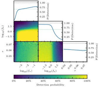
Additionally, our 1,000,000 evaluations allow for a broad range of further analyses at little to no additional computation cost. Instead of performing the average over in equation 8, we can marginalize over conditional priors with one or two parameters fixed, giving insight into under which early Universe astrophysical scenarios we would expect to detect the 21-cm signal. These conditional detection probabilities are depicted in figure 1 for the parameters with which strong variation in detection probability was seen, , , and . We find the detection of the 21-cm signal is more likely for high star formation efficiencies, X-ray efficiencies below a threshold of , and lower optical depths to reionization. With an almost 100% chance of a 3 detection for and . This strong variation in definitive detection chances retroactively provides further motivation for fully Bayesian forecasts as we see the conclusion drawn would be highly sensitive to the fiducial global 21-cm signal parameters chosen for a traditional Bayesian forecast.
There are a myriad of further analyses we could perform with our methodology. For example, we could study the evolution of the detection probability against the significance threshold, noise level or experiment bandwidth. Additionally, we could consider the functional distribution of the detected and non-detected 21-cm global signals to gain insight into what differentiates these two categories. Or alternatively, we could investigate how the chances of a 21-cm global signal detection have changed in light of the parameter constraints from the HERA 21-cm power spectrum limits [45, 46], or the SARAS 3 null detection [34, 47]. However, we shall leave these analyses to future work since the focus of this letter is on the method and its feasibility rather than particular scientific problems.
Let us return now to the computational performance of our method. The training data generation, network training, forecast data generation, network evaluations, and plotting of figure 1, took a combined total of 0.170 GPU hours 222On an NVIDIA A100-SXM-80GB GPU that was part of a CSD3 HPC Ampere GPU node.. Conversely, the 1000 polychord evaluations of as part of our validation process took a total of 778 CPU hours 333On 76 Intel Ice Lake CPUs that form a CSD3 HPC Ice Lake node., from which we can estimate the 1,000,000 evaluations used in our fully Bayesian forecast would have required 778,000 CPU hours using traditional methods. While it is not meaningful to directly compare GPU to CPU hours we can compare the costs of those hours. On the cluster we utilized GPU hours are charged at 50 times the rate of CPU hours. Thus our method gives a cost-weighted performance improvement of . Since this performance gain was for a single problem, and our implementation was not optimized, this level of performance gain cannot be assumed to apply universally. However, it is indicative our methodology is highly performant compared to traditional techniques and, as we have directly demonstrated, facilitates analyses that were previously computationally prohibitively expensive.
Conclusions.— We have argued that to arrive at accurate and interpretable predictions the conclusions of scientific forecasts should be marginalized over any uncertain model parameters and noise realizations. However, such fully Bayesian forecasts are computationally infeasible with traditional methods. We thus propose a novel methodology for performing fully Bayesian forecasts based on Evidence Networks.
To illustrate our method and the insights that can be gained from fully Bayesian forecasts, we applied it to determine the chances of a REACH-like experiment detecting the global 21-cm signal. For a frequency resolution of MHz and a noise level of K, we find a 65.2% (52.3%) chance of detection at 3 (5 ). Thus suggesting this noise level is indicative of the minimum sensitivity global 21-cm signal experiments should target. Additionally, our methodology allows us to produce triangle plots of how this chance of detection varies when one or two model parameters are fixed, at no extra computational cost. For this example problem, we find a cost-weighted speed-up of using our approach compared to a traditional nested-sampling-based method that would have taken CPU hours.
The method we propose can be applied to any forecasting question which can be formulated as a condition on the Bayes ratio between two models. This includes: if a signal can be detected from within noise (e.g. gravitational waves [50], or the 21-cm signal [29]); whether two competing theories can be distinguished by anticipated data (e.g. MOND [51] or General Relativity [52]); or if the inclusion of novel physics in a model will be necessary (e.g. neutrinos in CMB experiment analysis [15]). Additionally, the method only requires simulators of mock data, and thus can still be used in cases where closed-form likelihoods or explicit priors are not available. As a result, this methodology should allow for reliable and efficient fully Bayesian forecasts on a wide range of forecasting problems.
Since the proposed methodology is simulation-based and has a low computational cost, we anticipate it will be particularly suited to performing forecasts for a range of potential experimental configurations. Thus allowing for the optimization of experimental configurations to minimize cost or maximize the chance of the detection of new physics. To facilitate the application of this methodology by others we make public on GitHub all codes and data used in the writing of this letter.
Acknowledgements.
We would like to express our gratitude to Harry Bevins for several insightful conversations concerning this work. The authors would like to thank the Science and Technology Facilities Council (UK) for their support of TGJ through grant number ST/V506606/1, and the Royal Society for their support of WJH through a Royal Society University Research Fellowship. This work was performed using resources provided by the Cambridge Service for Data Driven Discovery (CSD3) operated by the University of Cambridge Research Computing Service (www.csd3.cam.ac.uk), provided by Dell EMC and Intel using Tier-2 funding from the Engineering and Physical Sciences Research Council (capital grant EP/T022159/1), and DiRAC funding from the Science and Technology Facilities Council (www.dirac.ac.uk). For the purpose of open access, the author has applied a Creative Commons Attribution (CC BY) licence to any Author Accepted Manuscript version arising from this submission.References
- Fisher [1922] R. A. Fisher, Philosophical Transactions of the Royal Society of London Series A 222, 309 (1922).
- Trotta [2007a] R. Trotta, MNRAS 378, 819 (2007a), arXiv:astro-ph/0703063 [astro-ph] .
- Sellentin et al. [2014] E. Sellentin, M. Quartin, and L. Amendola, MNRAS 441, 1831 (2014), arXiv:1401.6892 [astro-ph.CO] .
- Ryan et al. [2023] J. Ryan, B. Stevenson, C. Trendafilova, and J. Meyers, Phys. Rev. D 107, 103506 (2023), arXiv:2211.06534 [astro-ph.CO] .
- Anstey et al. [2021] D. Anstey, E. de Lera Acedo, and W. Handley, MNRAS 506, 2041 (2021), arXiv:2010.09644 [astro-ph.IM] .
- Rieck et al. [2023] S. Rieck, A. W. Criswell, V. Korol, M. A. Keim, and V. Mandic, arXiv e-prints , arXiv:2308.12437 (2023), arXiv:astro-ph/2308.12437 [astro-ph] .
- Tegmark et al. [1997] M. Tegmark, A. N. Taylor, and A. F. Heavens, ApJ 480, 22 (1997), arXiv:astro-ph/9603021 [astro-ph] .
- Albrecht et al. [2006] A. Albrecht, G. Bernstein, R. Cahn, W. L. Freedman, J. Hewitt, W. Hu, J. Huth, M. Kamionkowski, E. W. Kolb, L. Knox, J. C. Mather, S. Staggs, and N. B. Suntzeff, arXiv e-prints , astro-ph/0609591 (2006), arXiv:astro-ph/0609591 [astro-ph] .
- Seo and Eisenstein [2007] H.-J. Seo and D. J. Eisenstein, ApJ 665, 14 (2007), arXiv:astro-ph/0701079 [astro-ph] .
- Vallisneri [2008] M. Vallisneri, Phys. Rev. D 77, 042001 (2008), arXiv:gr-qc/0703086 [gr-qc] .
- More et al. [2013] S. More, F. C. van den Bosch, M. Cacciato, A. More, H. Mo, and X. Yang, MNRAS 430, 747 (2013), arXiv:1207.0004 [astro-ph.CO] .
- Di Dio et al. [2014] E. Di Dio, F. Montanari, R. Durrer, and J. Lesgourgues, J. Cosmology Astropart. Phys 2014, 042 (2014), arXiv:1308.6186 [astro-ph.CO] .
- Zhai and Blanton [2017] Z. Zhai and M. R. Blanton, ApJ 850, 41 (2017), arXiv:1707.06555 [astro-ph.CO] .
- Bonvin and Fleury [2018] C. Bonvin and P. Fleury, J. Cosmology Astropart. Phys 2018, 061 (2018), arXiv:1803.02771 [astro-ph.CO] .
- Ade et al. [2019] P. Ade, J. Aguirre, Z. Ahmed, S. Aiola, A. Ali, D. Alonso, M. A. Alvarez, K. Arnold, P. Ashton, J. Austermann, H. Awan, C. Baccigalupi, T. Baildon, D. Barron, N. Battaglia, R. Battye, E. Baxter, A. Bazarko, J. A. Beall, R. Bean, D. Beck, S. Beckman, B. Beringue, F. Bianchini, S. Boada, D. Boettger, J. R. Bond, J. Borrill, M. L. Brown, S. M. Bruno, S. Bryan, E. Calabrese, V. Calafut, P. Calisse, J. Carron, A. Challinor, G. Chesmore, Y. Chinone, J. Chluba, H.-M. S. Cho, S. Choi, G. Coppi, N. F. Cothard, K. Coughlin, D. Crichton, K. D. Crowley, K. T. Crowley, A. Cukierman, J. M. D’Ewart, R. Dünner, T. de Haan, M. Devlin, S. Dicker, J. Didier, M. Dobbs, B. Dober, C. J. Duell, S. Duff, A. Duivenvoorden, J. Dunkley, J. Dusatko, J. Errard, G. Fabbian, S. Feeney, S. Ferraro, P. Fluxà, K. Freese, J. C. Frisch, A. Frolov, G. Fuller, B. Fuzia, N. Galitzki, P. A. Gallardo, J. Tomas Galvez Ghersi, J. Gao, E. Gawiser, M. Gerbino, V. Gluscevic, N. Goeckner-Wald, J. Golec, S. Gordon, M. Gralla, D. Green, A. Grigorian, J. Groh, C. Groppi, Y. Guan, J. E. Gudmundsson, D. Han, P. Hargrave, M. Hasegawa, M. Hasselfield, M. Hattori, V. Haynes, M. Hazumi, Y. He, E. Healy, S. W. Henderson, C. Hervias-Caimapo, C. A. Hill, J. C. Hill, G. Hilton, M. Hilton, A. D. Hincks, G. Hinshaw, R. Hložek, S. Ho, S.-P. P. Ho, L. Howe, Z. Huang, J. Hubmayr, K. Huffenberger, J. P. Hughes, A. Ijjas, M. Ikape, K. Irwin, A. H. Jaffe, B. Jain, O. Jeong, D. Kaneko, E. D. Karpel, N. Katayama, B. Keating, S. S. Kernasovskiy, R. Keskitalo, T. Kisner, K. Kiuchi, J. Klein, K. Knowles, B. Koopman, A. Kosowsky, N. Krachmalnicoff, S. E. Kuenstner, C.-L. Kuo, A. Kusaka, J. Lashner, A. Lee, E. Lee, D. Leon, J. S. Y. Leung, A. Lewis, Y. Li, Z. Li, M. Limon, E. Linder, C. Lopez-Caraballo, T. Louis, L. Lowry, M. Lungu, M. Madhavacheril, D. Mak, F. Maldonado, H. Mani, B. Mates, F. Matsuda, L. Maurin, P. Mauskopf, A. May, N. McCallum, C. McKenney, J. McMahon, P. D. Meerburg, J. Meyers, A. Miller, M. Mirmelstein, K. Moodley, M. Munchmeyer, C. Munson, S. Naess, F. Nati, M. Navaroli, L. Newburgh, H. N. Nguyen, M. Niemack, H. Nishino, J. Orlowski-Scherer, L. Page, B. Partridge, J. Peloton, F. Perrotta, L. Piccirillo, G. Pisano, D. Poletti, R. Puddu, G. Puglisi, C. Raum, C. L. Reichardt, M. Remazeilles, Y. Rephaeli, D. Riechers, F. Rojas, A. Roy, S. Sadeh, Y. Sakurai, M. Salatino, M. Sathyanarayana Rao, E. Schaan, M. Schmittfull, N. Sehgal, J. Seibert, U. Seljak, B. Sherwin, M. Shimon, C. Sierra, J. Sievers, P. Sikhosana, M. Silva-Feaver, S. M. Simon, A. Sinclair, P. Siritanasak, K. Smith, S. R. Smith, D. Spergel, S. T. Staggs, G. Stein, J. R. Stevens, R. Stompor, A. Suzuki, O. Tajima, S. Takakura, G. Teply, D. B. Thomas, B. Thorne, R. Thornton, H. Trac, C. Tsai, C. Tucker, J. Ullom, S. Vagnozzi, A. van Engelen, J. Van Lanen, D. D. Van Winkle, E. M. Vavagiakis, C. Vergès, M. Vissers, K. Wagoner, S. Walker, J. Ward, B. Westbrook, N. Whitehorn, J. Williams, J. Williams, E. J. Wollack, Z. Xu, B. Yu, C. Yu, F. Zago, H. Zhang, N. Zhu, and Simons Observatory Collaboration, J. Cosmology Astropart. Phys 2019, 056 (2019), arXiv:1808.07445 [astro-ph.CO] .
- Euclid Collaboration et al. [2020] Euclid Collaboration, A. Blanchard, S. Camera, C. Carbone, V. F. Cardone, S. Casas, S. Clesse, S. Ilić, M. Kilbinger, T. Kitching, M. Kunz, F. Lacasa, E. Linder, E. Majerotto, K. Markovič, M. Martinelli, V. Pettorino, A. Pourtsidou, Z. Sakr, A. G. Sánchez, D. Sapone, I. Tutusaus, S. Yahia-Cherif, V. Yankelevich, S. Andreon, H. Aussel, A. Balaguera-Antolínez, M. Baldi, S. Bardelli, R. Bender, A. Biviano, D. Bonino, A. Boucaud, E. Bozzo, E. Branchini, S. Brau-Nogue, M. Brescia, J. Brinchmann, C. Burigana, R. Cabanac, V. Capobianco, A. Cappi, J. Carretero, C. S. Carvalho, R. Casas, F. J. Castander, M. Castellano, S. Cavuoti, A. Cimatti, R. Cledassou, C. Colodro-Conde, G. Congedo, C. J. Conselice, L. Conversi, Y. Copin, L. Corcione, J. Coupon, H. M. Courtois, M. Cropper, A. Da Silva, S. de la Torre, D. Di Ferdinando, F. Dubath, F. Ducret, C. A. J. Duncan, X. Dupac, S. Dusini, G. Fabbian, M. Fabricius, S. Farrens, P. Fosalba, S. Fotopoulou, N. Fourmanoit, M. Frailis, E. Franceschi, P. Franzetti, M. Fumana, S. Galeotta, W. Gillard, B. Gillis, C. Giocoli, P. Gómez-Alvarez, J. Graciá-Carpio, F. Grupp, L. Guzzo, H. Hoekstra, F. Hormuth, H. Israel, K. Jahnke, E. Keihanen, S. Kermiche, C. C. Kirkpatrick, R. Kohley, B. Kubik, H. Kurki-Suonio, S. Ligori, P. B. Lilje, I. Lloro, D. Maino, E. Maiorano, O. Marggraf, N. Martinet, F. Marulli, R. Massey, E. Medinaceli, S. Mei, Y. Mellier, B. Metcalf, J. J. Metge, G. Meylan, M. Moresco, L. Moscardini, E. Munari, R. C. Nichol, S. Niemi, A. A. Nucita, C. Padilla, S. Paltani, F. Pasian, W. J. Percival, S. Pires, G. Polenta, M. Poncet, L. Pozzetti, G. D. Racca, F. Raison, A. Renzi, J. Rhodes, E. Romelli, M. Roncarelli, E. Rossetti, R. Saglia, P. Schneider, V. Scottez, A. Secroun, G. Sirri, L. Stanco, J. L. Starck, F. Sureau, P. Tallada-Crespí, D. Tavagnacco, A. N. Taylor, M. Tenti, I. Tereno, R. Toledo-Moreo, F. Torradeflot, L. Valenziano, T. Vassallo, G. A. Verdoes Kleijn, M. Viel, Y. Wang, A. Zacchei, J. Zoubian, and E. Zucca, A&A 642, A191 (2020), arXiv:1910.09273 [astro-ph.CO] .
- d’Assignies D et al. [2023] W. d’Assignies D, C. Zhao, J. Yu, and J.-P. Kneib, MNRAS 521, 3648 (2023), arXiv:2301.02289 [astro-ph.CO] .
- Mason et al. [2023] C. A. Mason, J. B. Muñoz, B. Greig, A. Mesinger, and J. Park, MNRAS 524, 4711 (2023), arXiv:2212.09797 [astro-ph.CO] .
- Perotto et al. [2006] L. Perotto, J. Lesgourgues, S. Hannestad, H. Tu, and Y. Y Y Wong, J. Cosmology Astropart. Phys 2006, 013 (2006), arXiv:astro-ph/0606227 [astro-ph] .
- Wolz et al. [2012] L. Wolz, M. Kilbinger, J. Weller, and T. Giannantonio, J. Cosmology Astropart. Phys 2012, 009 (2012), arXiv:1205.3984 [astro-ph.CO] .
- Trotta [2007b] R. Trotta, MNRAS 378, 72 (2007b), arXiv:astro-ph/0504022 [astro-ph] .
- Jeffrey and Wandelt [2023] N. Jeffrey and B. D. Wandelt, arXiv e-prints , arXiv:2305.11241 (2023), arXiv:2305.11241 [cs.LG] .
- de Lera Acedo et al. [2022] E. de Lera Acedo, D. I. L. de Villiers, N. Razavi-Ghods, W. Handley, A. Fialkov, A. Magro, D. Anstey, H. T. J. Bevins, R. Chiello, J. Cumner, A. T. Josaitis, I. L. V. Roque, P. H. Sims, K. H. Scheutwinkel, P. Alexander, G. Bernardi, S. Carey, J. Cavillot, W. Croukamp, J. A. Ely, T. Gessey-Jones, Q. Gueuning, R. Hills, G. Kulkarni, R. Maiolino, P. D. Meerburg, S. Mittal, J. R. Pritchard, E. Puchwein, A. Saxena, E. Shen, O. Smirnov, M. Spinelli, and K. Zarb-Adami, Nature Astronomy 6, 984 (2022).
- MacKay [2003] D. MacKay, Information Theory, Inference and Learning Algorithms (Cambridge University Press, 2003).
- Skilling [2004] J. Skilling, in Bayesian Inference and Maximum Entropy Methods in Science and Engineering: 24th International Workshop on Bayesian Inference and Maximum Entropy Methods in Science and Engineering, American Institute of Physics Conference Series, Vol. 735, edited by R. Fischer, R. Preuss, and U. V. Toussaint (2004) pp. 395–405.
- Ashton et al. [2022] G. Ashton, N. Bernstein, J. Buchner, X. Chen, G. Csányi, A. Fowlie, F. Feroz, M. Griffiths, W. Handley, M. Habeck, E. Higson, M. Hobson, A. Lasenby, D. Parkinson, L. B. Pártay, M. Pitkin, D. Schneider, J. S. Speagle, L. South, J. Veitch, P. Wacker, D. J. Wales, and D. Yallup, Nature Reviews Methods Primers 2, 39 (2022), arXiv:2205.15570 [stat.CO] .
- Dickey [1971] J. M. Dickey, The Annals of Mathematical Statistics 42, 204 (1971).
- Verdinelli and Wasserman [1995] I. Verdinelli and L. Wasserman, Journal of the American Statistical Association 90, 614 (1995).
- Furlanetto et al. [2006] S. R. Furlanetto, S. P. Oh, and F. H. Briggs, Phys. Rep. 433, 181 (2006), arXiv:astro-ph/0608032 [astro-ph] .
- Bowman et al. [2018] J. D. Bowman, A. E. E. Rogers, R. A. Monsalve, T. J. Mozdzen, and N. Mahesh, Nature 555, 67 (2018), arXiv:1810.05912 [astro-ph.CO] .
- Hills et al. [2018] R. Hills, G. Kulkarni, P. D. Meerburg, and E. Puchwein, Nature 564, E32 (2018), arXiv:1805.01421 [astro-ph.CO] .
- Barkana [2018] R. Barkana, Nature 555, 71 (2018), arXiv:1803.06698 [astro-ph.CO] .
- Sims and Pober [2020] P. H. Sims and J. C. Pober, MNRAS 492, 22 (2020), arXiv:1910.03165 [astro-ph.CO] .
- Singh et al. [2022] S. Singh, N. T. Jishnu, R. Subrahmanyan, N. Udaya Shankar, B. S. Girish, A. Raghunathan, R. Somashekar, K. S. Srivani, and M. Sathyanarayana Rao, Nature Astronomy 6, 607 (2022), arXiv:2112.06778 [astro-ph.CO] .
- Philip et al. [2019] L. Philip, Z. Abdurashidova, H. C. Chiang, N. Ghazi, A. Gumba, H. M. Heilgendorff, J. M. Jáuregui-García, K. Malepe, C. D. Nunhokee, J. Peterson, J. L. Sievers, V. Simes, and R. Spann, Journal of Astronomical Instrumentation 8, 1950004 (2019).
- Note [1] As the noise scales with spectral resolution as this is equivalent to K noise at a resolution of MHz, the pessimistic case projected for REACH [23].
- Bevins et al. [2021] H. T. J. Bevins, W. J. Handley, A. Fialkov, E. de Lera Acedo, and K. Javid, MNRAS 508, 2923 (2021), arXiv:2104.04336 [astro-ph.CO] .
- Visbal et al. [2012] E. Visbal, R. Barkana, A. Fialkov, D. Tseliakhovich, and C. M. Hirata, Nature 487, 70 (2012), arXiv:1201.1005 [astro-ph.CO] .
- Fialkov et al. [2014] A. Fialkov, R. Barkana, A. Pinhas, and E. Visbal, MNRAS 437, L36 (2014), arXiv:1306.2354 [astro-ph.CO] .
- Reis et al. [2020] I. Reis, A. Fialkov, and R. Barkana, MNRAS 499, 5993 (2020), arXiv:2008.04315 [astro-ph.CO] .
- Planck Collaboration et al. [2020] Planck Collaboration, N. Aghanim, Y. Akrami, M. Ashdown, J. Aumont, C. Baccigalupi, M. Ballardini, A. J. Banday, R. B. Barreiro, N. Bartolo, S. Basak, R. Battye, K. Benabed, J. P. Bernard, M. Bersanelli, P. Bielewicz, J. J. Bock, J. R. Bond, J. Borrill, F. R. Bouchet, F. Boulanger, M. Bucher, C. Burigana, R. C. Butler, E. Calabrese, J. F. Cardoso, J. Carron, A. Challinor, H. C. Chiang, J. Chluba, L. P. L. Colombo, C. Combet, D. Contreras, B. P. Crill, F. Cuttaia, P. de Bernardis, G. de Zotti, J. Delabrouille, J. M. Delouis, E. Di Valentino, J. M. Diego, O. Doré, M. Douspis, A. Ducout, X. Dupac, S. Dusini, G. Efstathiou, F. Elsner, T. A. Enßlin, H. K. Eriksen, Y. Fantaye, M. Farhang, J. Fergusson, R. Fernandez-Cobos, F. Finelli, F. Forastieri, M. Frailis, A. A. Fraisse, E. Franceschi, A. Frolov, S. Galeotta, S. Galli, K. Ganga, R. T. Génova-Santos, M. Gerbino, T. Ghosh, J. González-Nuevo, K. M. Górski, S. Gratton, A. Gruppuso, J. E. Gudmundsson, J. Hamann, W. Handley, F. K. Hansen, D. Herranz, S. R. Hildebrandt, E. Hivon, Z. Huang, A. H. Jaffe, W. C. Jones, A. Karakci, E. Keihänen, R. Keskitalo, K. Kiiveri, J. Kim, T. S. Kisner, L. Knox, N. Krachmalnicoff, M. Kunz, H. Kurki-Suonio, G. Lagache, J. M. Lamarre, A. Lasenby, M. Lattanzi, C. R. Lawrence, M. Le Jeune, P. Lemos, J. Lesgourgues, F. Levrier, A. Lewis, M. Liguori, P. B. Lilje, M. Lilley, V. Lindholm, M. López-Caniego, P. M. Lubin, Y. Z. Ma, J. F. Macías-Pérez, G. Maggio, D. Maino, N. Mandolesi, A. Mangilli, A. Marcos-Caballero, M. Maris, P. G. Martin, M. Martinelli, E. Martínez-González, S. Matarrese, N. Mauri, J. D. McEwen, P. R. Meinhold, A. Melchiorri, A. Mennella, M. Migliaccio, M. Millea, S. Mitra, M. A. Miville-Deschênes, D. Molinari, L. Montier, G. Morgante, A. Moss, P. Natoli, H. U. Nørgaard-Nielsen, L. Pagano, D. Paoletti, B. Partridge, G. Patanchon, H. V. Peiris, F. Perrotta, V. Pettorino, F. Piacentini, L. Polastri, G. Polenta, J. L. Puget, J. P. Rachen, M. Reinecke, M. Remazeilles, A. Renzi, G. Rocha, C. Rosset, G. Roudier, J. A. Rubiño-Martín, B. Ruiz-Granados, L. Salvati, M. Sandri, M. Savelainen, D. Scott, E. P. S. Shellard, C. Sirignano, G. Sirri, L. D. Spencer, R. Sunyaev, A. S. Suur-Uski, J. A. Tauber, D. Tavagnacco, M. Tenti, L. Toffolatti, M. Tomasi, T. Trombetti, L. Valenziano, J. Valiviita, B. Van Tent, L. Vibert, P. Vielva, F. Villa, N. Vittorio, B. D. Wandelt, I. K. Wehus, M. White, S. D. M. White, A. Zacchei, and A. Zonca, A&A 641, A6 (2020), arXiv:1807.06209 [astro-ph.CO] .
- Abadi et al. [2015] M. Abadi, A. Agarwal, P. Barham, E. Brevdo, Z. Chen, C. Citro, G. S. Corrado, A. Davis, J. Dean, M. Devin, S. Ghemawat, I. Goodfellow, A. Harp, G. Irving, M. Isard, Y. Jia, R. Jozefowicz, L. Kaiser, M. Kudlur, J. Levenberg, D. Mané, R. Monga, S. Moore, D. Murray, C. Olah, M. Schuster, J. Shlens, B. Steiner, I. Sutskever, K. Talwar, P. Tucker, V. Vanhoucke, V. Vasudevan, F. Viégas, O. Vinyals, P. Warden, M. Wattenberg, M. Wicke, Y. Yu, and X. Zheng, TensorFlow: Large-scale machine learning on heterogeneous systems (2015), software available from tensorflow.org.
- Handley et al. [2015a] W. J. Handley, M. P. Hobson, and A. N. Lasenby, MNRAS 450, L61 (2015a), arXiv:1502.01856 [astro-ph.CO] .
- Handley et al. [2015b] W. J. Handley, M. P. Hobson, and A. N. Lasenby, MNRAS 453, 4384 (2015b), arXiv:1506.00171 [astro-ph.IM] .
- Abdurashidova et al. [2022] Z. Abdurashidova, J. E. Aguirre, P. Alexander, Z. S. Ali, Y. Balfour, R. Barkana, A. P. Beardsley, G. Bernardi, T. S. Billings, J. D. Bowman, R. F. Bradley, P. Bull, J. Burba, S. Carey, C. L. Carilli, C. Cheng, D. R. DeBoer, M. Dexter, E. de Lera Acedo, J. S. Dillon, J. Ely, A. Ewall-Wice, N. Fagnoni, A. Fialkov, R. Fritz, S. R. Furlanetto, K. Gale-Sides, B. Glendenning, D. Gorthi, B. Greig, J. Grobbelaar, Z. Halday, B. J. Hazelton, S. Heimersheim, J. N. Hewitt, J. Hickish, D. C. Jacobs, A. Julius, N. S. Kern, J. Kerrigan, P. Kittiwisit, S. A. Kohn, M. Kolopanis, A. Lanman, P. La Plante, T. Lekalake, D. Lewis, A. Liu, Y.-Z. Ma, D. MacMahon, L. Malan, C. Malgas, M. Maree, Z. E. Martinot, E. Matsetela, A. Mesinger, J. Mirocha, M. Molewa, M. F. Morales, T. Mosiane, J. B. Muñoz, S. G. Murray, A. R. Neben, B. Nikolic, C. D. Nunhokee, A. R. Parsons, N. Patra, S. Pieterse, J. C. Pober, Y. Qin, N. Razavi-Ghods, I. Reis, J. Ringuette, J. Robnett, K. Rosie, M. G. Santos, S. Sikder, P. Sims, C. Smith, A. Syce, N. Thyagarajan, P. K. G. Williams, and H. Zheng, ApJ 924, 51 (2022), arXiv:2108.07282 [astro-ph.CO] .
- HERA Collaboration et al. [2023] HERA Collaboration, Z. Abdurashidova, T. Adams, J. E. Aguirre, P. Alexander, Z. S. Ali, R. Baartman, Y. Balfour, R. Barkana, A. P. Beardsley, G. Bernardi, T. S. Billings, J. D. Bowman, R. F. Bradley, D. Breitman, P. Bull, J. Burba, S. Carey, C. L. Carilli, C. Cheng, S. Choudhuri, D. R. DeBoer, E. de Lera Acedo, M. Dexter, J. S. Dillon, J. Ely, A. Ewall-Wice, N. Fagnoni, A. Fialkov, R. Fritz, S. R. Furlanetto, K. Gale-Sides, H. Garsden, B. Glendenning, A. Gorce, D. Gorthi, B. Greig, J. Grobbelaar, Z. Halday, B. J. Hazelton, S. Heimersheim, J. N. Hewitt, J. Hickish, D. C. Jacobs, A. Julius, N. S. Kern, J. Kerrigan, P. Kittiwisit, S. A. Kohn, M. Kolopanis, A. Lanman, P. La Plante, D. Lewis, A. Liu, A. Loots, Y.-Z. Ma, D. H. E. MacMahon, L. Malan, K. Malgas, C. Malgas, M. Maree, B. Marero, Z. E. Martinot, L. McBride, A. Mesinger, J. Mirocha, M. Molewa, M. F. Morales, T. Mosiane, J. B. Muñoz, S. G. Murray, V. Nagpal, A. R. Neben, B. Nikolic, C. D. Nunhokee, H. Nuwegeld, A. R. Parsons, R. Pascua, N. Patra, S. Pieterse, Y. Qin, N. Razavi-Ghods, J. Robnett, K. Rosie, M. G. Santos, P. Sims, S. Singh, C. Smith, H. Swarts, J. Tan, N. Thyagarajan, M. J. Wilensky, P. K. G. Williams, P. van Wyngaarden, and H. Zheng, ApJ 945, 124 (2023).
- Bevins et al. [2022] H. T. J. Bevins, A. Fialkov, E. de Lera Acedo, W. J. Handley, S. Singh, R. Subrahmanyan, and R. Barkana, Nature Astronomy 6, 1473 (2022), arXiv:2212.00464 [astro-ph.CO] .
- Note [2] On an NVIDIA A100-SXM-80GB GPU that was part of a CSD3 HPC Ampere GPU node.
- Note [3] On 76 Intel Ice Lake CPUs that form a CSD3 HPC Ice Lake node.
- Evans et al. [2023] M. Evans, A. Corsi, C. Afle, A. Ananyeva, K. G. Arun, S. Ballmer, A. Bandopadhyay, L. Barsotti, M. Baryakhtar, E. Berger, E. Berti, S. Biscoveanu, S. Borhanian, F. Broekgaarden, D. A. Brown, C. Cahillane, L. Campbell, H.-Y. Chen, K. J. Daniel, A. Dhani, J. C. Driggers, A. Effler, R. Eisenstein, S. Fairhurst, J. Feicht, P. Fritschel, P. Fulda, I. Gupta, E. D. Hall, G. Hammond, O. A. Hannuksela, H. Hansen, C.-J. Haster, K. Kacanja, B. Kamai, R. Kashyap, J. Shapiro Key, S. Khadkikar, A. Kontos, K. Kuns, M. Landry, P. Landry, B. Lantz, T. G. F. Li, G. Lovelace, V. Mandic, G. L. Mansell, D. Martynov, L. McCuller, A. L. Miller, A. H. Nitz, B. J. Owen, C. Palomba, J. Read, H. Phurailatpam, S. Reddy, J. Richardson, J. Rollins, J. D. Romano, B. S. Sathyaprakash, R. Schofield, D. H. Shoemaker, D. Sigg, D. Singh, B. Slagmolen, P. Sledge, J. Smith, M. Soares-Santos, A. Strunk, L. Sun, D. Tanner, L. A. C. van Son, S. Vitale, B. Willke, H. Yamamoto, and M. Zucker, arXiv e-prints , arXiv:2306.13745 (2023), arXiv:2306.13745 [astro-ph.IM] .
- Milgrom [1983] M. Milgrom, ApJ 270, 365 (1983).
- Wald [1984] R. M. Wald, General Relativity (University of Chicago Press, 1984).