Near Real-Time Gravitational Wave Data Analysis of the Massive Black Hole Binary with TianQin

Abstract

Space-borne gravitational wave detectors can detect sources like the merger of massive black holes. The rapid identification and localization of the source would play a crucial role in multi-messenger observation. The geocentric orbit of the space-borne gravitational wave detector, TianQin, makes it possible to conduct real-time data transmission. In this manuscript, we develop a search and localization pipeline for massive black hole binaries with TianQin, under both regular and real-time data transmission modes. We demonstrate that with real-time data transmission, it is possible to accurately localize the massive black hole binaries on-the-fly. With the approaching of the merger, the localization rapidly shrinks, and the data analysis can be finished at a speed comparable to the data downlink speed.

I Introduction

The past years have witnessed significant progress of the field of gravitational wave (GW) astronomy, with nearly a hundred of GW events detected by ground-based GW detectors [1, 2, 3], and recently a number of pulsar timing arrays announced detection of $n{\rm Hz}$ stochastic GW backgrounds [4, 5, 6, 7]. Meanwhile, GW signals in the range of $0.1{\rm mHz}-1{\rm Hz}$ can be detected by space-borne GW detectors like TianQin [8] and Laser Interferometer Space Antenna (LISA) [9]. Potential sources range from massive black hole binarys [10], stellar mass black hole binarys [11], extreme mass-ratio inspirals [12], Galactic double white dwarfs [13], to stochastic gravitational-wave background (SGWB) [14].

Among these sources, MBHBs are expected to produce the loudest GW signals, with a signal-to-noise ratio (SNR) of up to several thousand. Depending on different models of formation and evolution of massive black holes [15, 16, 17], MBHBs may be observable as early as $z\simeq 15\sim 20$.

MBHBs can merge in gas-rich environments [18] and result in a high black hole accretion rate (BHAR) and high star formation rate (SFR) in the galaxy [19, 20]. Both of these factors have the potential to cause strong electromagnetic (EM) radiation, making MBHBs promising targets for multi-messenger astronomy. During the inspiral phase, EM emission from MBHBs is predominantly from X-rays emitted by the circumbinary disk [21], but then gradually decline prior to merger [22], and shift towards being dominated by ultraviolet (UV) radiation as the merger approaches [23]. At the moment of the merger, we anticipate a variety of EM emissions, such as a super-Eddington flare from the super-Eddington accretion rate [24, 25], X-ray emission from the spin flip of the black hole [26], as well as jets caused by surrounding magnetic field [27, 28]. Additionally, with delays ranging from hours to months after the coalescence, we may observe highly relativistic jets launched along the black hole’s spin axis [29]. Even long after the merger, various EM afterglows are expected to persist [30, 31, 32].

In recent years, there has been a significant amount of research focused on studying GW and EM multi-messenger observations involving MBHBs [33, 34]. The primary focus of attention has been on the localization capability of GW detectors for MBHBs, as well as the anticipated outcomes of joint observations with multi-band EM facilities, such as the Large Synoptic Survey Telescope (LSST) [35, 36] and the Extremely Large Telescope (ELT) [37] in optical, the Advanced Telescope for High Energy Astrophysics (Athena) [38] in X-ray, and the Square Kilometre Array (SKA) [39] in radio.

GW observations can provide us with information about the masses and spins of MBHBs, while EM observations can give us insight into the environment around massive black holes and reveal the behavior of the accretion disks around the MBHBs, particularly at late times in their inspiral evolution [40, 41]. Multi-messenger observations of MBHBs will enable us to gain knowledge about the co-evolution of massive black holes, nuclear star clusters, and their host galaxies [17, 42], shedding light on the time delay between galaxy merger and MBHBs merger, as well as the physics of active galactic nuclei (AGN) [43]. Moreover, the direct measurement of luminosity distance by GW analysis and the inference of redshift by EM analysis can provide a new measure of the Hubble parameter [44, 45] and constrain cosmological extra dimensions [46]. By comparing the phases of GW and EM signals to break the degeneracies of various parameters, the fractional difference in propagation velocity between gravitons and photons can be accurately determined to $10^{-17}$ [47].

Despite the promising potential for multi-messenger observations of MBHBs, observing the EM signal from MBHB mergers poses a number of challenges, primarily due to the short emission timescale. The typical long distance to the source also results in faint emissions. Another challenge associated with observing MBHBs is the gravitational lensing, which can significantly distort and attenuate the emission, making it difficult to accurately measure. Furthermore, distinguishing the radiation from background noise can be quite tricky. The identification of the source as a MBHB would require adequate evidence.

All of the aforementioned challenges can be addressed by localizing, and most importantly, conducting EM observations of MBHBs before the merger. However, the SNR of a MBHB accumulates in a highly non-linear way, the last hour signal contains up to 99% of the total SNR [48], and the sky localization area shrinks significantly as the MBHB approaches merger [34]. Therefore, the localization of MBHBs prior to the merger raised a new challenge of near real-time speed for the data downlink as well as for the data analysis.

Due to the relatively short distance from the Earth, TianQin has the potential to enable near real-time data transmission to Earth. In this work, we study how to analyse and localize the MBHBs prior to the merger, under the assumption that TianQin data can be transmitted real time. Due to the longer duration of signals, data analysis for space-borne GW detectors can be a lengthy process, taking days or even weeks with the calculation of the likelihood being a major bottleneck. To speed up the processing, various algorithms have been developed, such as heterodyned likelihood algorithm [49, 50, 51], reduced order quadratures [52], multi-banding likelihood method [53, 54] and so on. In this work, we used the heterodyned likelihood algorithm adapted from BBHx [55]. Furthermore, we have made some adjustments to the settings to better suit the near real-time analysis for TianQin.

The paper is organized as follows. In Section II, we describe the waveform of MBHBs with the response function of TianQin. In Section III, we describe the method used in this work. These methods will be applied to the analysis pipeline in Section IV. In Section V, we injected three signals to demonstrate the performance of the pipeline. Finally, the conclusion of this work and future directions for development are discussed in Section VI.

II Waveform of MBHB

Throughout the work, we adopt the aligned spin IMRPhenomD waveform for the MBHBs signal [56, 57]. The waveform is described by a set of parameters: $\Theta=\left\{M_{c},\eta,\chi_{1},\chi_{2},D_{L},t_{c},\phi_{c},\psi,\iota,\lambda,\beta\right\}$. $M_{c}$ is the redshifted chirp mass defined as $M_{c}=(m_{1}m_{2})^{3/5}/(m_{1}+m_{2})^{1/5}(1+z)$. In this work, we only consider MBHBs with redshifted chirp mass ranges between $10^{4}$ to $10^{8}$. $\eta=m_{1}m_{2}/(m_{1}+m_{2})^{2}$ is the symmetric mass ratio. Equal mass binaries have a $\eta=0.25$, and we set the lower limit of $\eta$ to $0.05$, which approximates the mass ratio of $1:18$. This corresponds to the parameter space where the IMRPhenomD waveforms are reliable. $\chi_{1}$ and $\chi_{2}$ ranging between $-1$ to $1$ are the dimensionless spins of the two black holes. $D_{L}$ is the luminosity distance, $t_{c}$ and $\phi_{c}$ are merger time and merge phase, respectively. $\psi$ is the polarization angle, and $\iota$ is the inclination angle that measures the angle between the binary’s angular momentum vector and the line of sight to the observer. Finally, we use $\lambda$ and $\beta$ to denote the ecliptic longitude and ecliptic latitude, respectively, of the source location.

Before generating the waveform, one has to determine the frequency range. The frequency evolution can be calculated with Newtonian approximation

$$f\left(t\right)=\frac{1}{8\pi}\left(\frac{c^{3}}{GM_{c}}\right)^{5/8}\left(\frac{t_{c}-t}{5}\right)^{-3/8},$$ (1)

If the MBHB merges within the observation period, then the upper limit of the frequency will be determined through

$$f_{\rm cut}=\frac{1}{5}\frac{c^{3}}{GM_{\rm tot}},$$ (2)

where, the $M_{\rm tot}$ is the total mass of the black holes binary. We also apply a truncate between $10^{-4}$ Hz and $1$ Hz according to the frequency limit of TianQin. In practice, we adopt pyIMRPhenomD [58] for generating the frequency domain amplitude $\mathcal{A}\left(f\right)$ and phase $\Phi\left(f\right)$, which allows for the analytical calculation of the time-frequency relation $t\left(f\right)$ and $t^{\prime}\left(f\right)$.

For space-borne GW missions, one of the dominating sources of noise is the laser frequency noise, which can be mitigated through the time delay interferometry (TDI) technology [59, 60]. Throughout this work, we adopt the commonly used orthogonal channels, namely $A,\ E,$ and noise-insensitive $T$. They can be combined through the symmetric TDI Michelson channels $X,\ Y,$ and $Z$ [60, 61]:

$$A =\frac{1}{\sqrt{2}}\left(Z-X\right),$$ (3a)

$$E =\frac{1}{\sqrt{6}}\left(X-2Y+Z\right),$$ (3b)

$$T =\frac{1}{\sqrt{3}}\left(X+Y+Z\right),$$ (3c)

Several TDI schemes have been proposed for space-borne GW detectors [62, 63, 64]. But they are merely modifications of the first-generation TDI and do not significantly alter the response. As a result, only the first-generation TDI will be utilized in this study. These observables can be represented by basic Doppler observables $\tilde{y}_{ij}$, which represents a laser frequency shift between different spacecraft [59, 60, 61].

We define $\tilde{A}$ as the Fourier transform of $A$. Taking account of the TianQin orbit [65], one can express the TDI response for TianQin of the TDI channels in frequency domain as [59],

$$\tilde{A}= {\rm i}\sqrt{2}\,x\sin\left(\frac{2\pi fL}{c}\right)\left[(1+x)\left(\tilde{y}_{31}+\tilde{y}_{13}\right)-\tilde{y}_{23}\right.$$

$$\left.-x\,\tilde{y}_{32}-\tilde{y}_{21}-x\,\tilde{y}_{12}\right],$$ (4a)

$$\tilde{E}= {\rm i}\frac{\sqrt{2}}{\sqrt{3}}\,x\sin\left(\frac{2\pi fL}{c}\right)\left[(1-x)\left(\tilde{y}_{13}-\tilde{y}_{31}\right)\right.$$

$$\left.+(2+x)\left(\tilde{y}_{12}-\tilde{y}_{32}\right)+(1+2x)\left(\tilde{y}_{21}-\tilde{y}_{23}\right)\right],$$ (4b)

$$\tilde{T}= \frac{4}{\sqrt{3}}\,x^{\frac{3}{2}}\sin\left(\frac{\pi fL}{c}\right)\sin\left(\frac{2\pi fL}{c}\right)\left[\tilde{y}_{21}-\tilde{y}_{12}\right.$$

$$\left.+\tilde{y}_{32}-\tilde{y}_{23}+\tilde{y}_{13}-\tilde{y}_{31}\right],$$ (4c)

where $x\equiv e^{\frac{{\rm i}2\pi fL}{c}}$. As the observables $T$ are insensitive to signal at low frequencies, we concentrate on the $A,E$ channels.

We then add the Doppler phase $\Phi_{R}$, which corresponds to the phase delay between the signal arrival at the Solar System Barycenter (SSB) and at the geometric centre of the constellation. Since TianQin adopts a geocentric orbit, it is simply the geocenter, and we can express the Doppler phase as

$$\Phi_{R}\left(f\right)=\frac{2\pi f}{c}\vec{k}\cdot\vec{p_{0}},$$ (5)

where $\vec{k}=\{-\cos\beta\cos\lambda,-\cos\beta\sin\lambda,-\sin\beta\}$ is the normalized wave vector, and $\vec{p_{0}}$ is the normalized vector pointing from the SSB to the Earth.

Finally, the signal can be represented as:

$$\tilde{h}_{A,E}=\mathcal{A}\left(f\right)e^{{\rm i}\left(\Phi\left(f\right)+\Phi_{R}\left(f\right)+2\pi ft_{c}\right)}\times\tilde{A},\tilde{E}.$$ (6)

III Method

III.1 Bayesian Framework

In this work, we adopt the Bayes framework to obtain the posterior distribution of the parameters $\Theta$. According to Bayes theorem, the posterior can be expressed as

$$p\left(\Theta\mid d,I\right)=\frac{p\left(d\mid\Theta,I\right)p\left(\Theta\mid I\right)}{p\left(d\mid I\right)},$$ (7)

$p\left(\Theta\mid d,I\right)$ is the posterior, $p\left(d\mid\Theta,I\right)$ is the likelihood, $p\left(\Theta\mid I\right)$ is the prior, and the normalizing $p\left(d\mid I\right)$ is the evidence, with $d$ being the observed data, and $I$ represent the information.

For GW data analysis, the likelihood can be expressed as

$$\log\mathcal{L}(\Theta)= \log p\left(d\mid\Theta,I\right)$$

$$= -\frac{1}{2}\langle d-h\left(\Theta\right)\mid d-h\left(\Theta\right)\rangle+{\rm const.}$$

$$= \langle d\mid h\left(\Theta\right)\rangle-\frac{1}{2}\langle h\left(\Theta\right)\mid h\left(\Theta\right)\rangle$$

$$-\frac{1}{2}\langle d\mid d\rangle+{\rm const.},$$ (8)

$h\left(\Theta\right)$ is the waveform with parameter $\Theta$, and $\langle g\mid h\rangle$ represents the inner product between $g$ and $h$

$$\langle g\mid h\rangle=4\Re\int_{0}^{\infty}\frac{\widetilde{g}\left(f\right)\cdot\widetilde{h}^{*}\left(f\right)}{S_{n}\left(f\right)}{\rm d}f,$$ (9)

with $S_{n}\left(f\right)$ being the one-sided power spectral density (PSD) of the noise, and $\Re$ is the real component.

The constant is related to the normalization of the Bayes equation. If we ignore all constant terms, the log-likelihood can be simplified as

$$\log\mathcal{L}(\Theta)\propto\langle d\mid h\rangle-\frac{1}{2}\langle h\mid h\rangle.$$ (10)

The analysis for GW signals involves high dimensional parameter space. To efficiently explore the parameter space, stochastic sampling methods like Markov Chain Monte Carlo (MCMC) are often used in the GW data analysis community. The MCMC method uses random walking of the sampler, and it encourages moves to the higher posterior region. In this work, we utilize emcee, a specific realization of the affine invariant ensemble sampler algorithm [66]. It enables multiple walkers, representing parameter vectors, to navigate through it by proposing new positions based on the posterior distribution. The use of multiple walkers enhances the robustness and effectiveness of MCMC sampling in complex, high-dimensional parameter spaces [67].

Traditionally, MCMC methods are only applied to the parameter estimation tasks, and the identification of the signal is often treated as a separate scope. However, in this work, we do not clearly distinguish the detection and measurement of GW signals. Instead, we first use the emcee sampler to efficiently explore the parameter space with accumulating data. Then we identify the walkers with significantly lower posteriors and replace them with points randomly perturbed around the maximum posterior sample. Finally, the parameter estimation results have been obtained by continuing sampling.

III.2 Heterodyned Likelihood

The overall time spent on the analysis is determined by two factors, the number of samples needed, and the average time it takes to generate a single waveform. In our analysis pipeline, we will leverage the heterodyned likelihood method [51, 49, 55] as part of our fast estimation module.

The core idea of the heterodyned likelihood method is to separate the waveform $\widetilde{h}(f)$ into two parts: a rapidly changing component which is common in the reference waveform $\widetilde{h}_{0}\left(f\right)$, and a slowly changing component that indicates the ratio $\widetilde{r}\left(f\right)=\frac{\widetilde{h}\left(f\right)}{\widetilde{h}_{0}\left(f\right)}$. Under this decomposition, one can expand the two inner products as

$$\langle d\mid h\rangle =4\Re\int_{0}^{\infty}\frac{\widetilde{d}\left(f\right)\cdot\widetilde{h}_{0}^{*}\left(f\right)}{S_{n}\left(f\right)}\times\widetilde{r}\left(f\right){\rm d}f,$$ (11a)

$$\langle h\mid h\rangle =4\Re\int_{0}^{\infty}\frac{\left|\widetilde{h}_{0}\left(f\right)\right|^{2}}{S_{n}\left(f\right)}\times\left|\widetilde{r}\left(f\right)\right|^{2}{\rm d}f,$$ (11b)

In practice, We first need to obtain a reference waveform $\widetilde{h}_{0}\left(f\right)$ with a high posterior. Then the rapidly changing components $\widetilde{d}\left(f\right)\widetilde{h}_{0}^{*}\left(f\right)/S_{n}\left(f\right)$ and $\left|\widetilde{h}_{0}\left(f\right)\right|^{2}/S_{n}\left(f\right)$ only need to be computed once and stored as a precomputed factor. In sampling, one only needs to calculate the waveform ratio $\widetilde{r}\left(f\right)$ (dubbed likelihood core) on a sparse frequency grid. In this way, the average time to compute the likelihood can be greatly reduced.

To quantify the efficiency improvement of the heterodyned likelihood method over ordinary likelihood, we generate a total of 4,000 different signals with different waveform lengths ranging from $10^{3}$ to $10^{6}$. We fix $M_{c}=3\times 10^{5}M_{\odot}$, and $D_{L}=1{\rm Gpc}$ and randomize over all other parameters. The 4,000 waveforms are generated with both methods and in Figure 1, we present the computing time for each case with a single CPU Intel Core i7-10700 @2.90GHz, with the lines cross the mean value and error bars indicate the 90 % confidence intervals. Here, the injected waveform is selected as the reference waveform for heterodyned likelihood. For shorter waveform lengths, the frequency is already sufficiently sparse, and the heterodyned likelihood method does not show a significant advantage against the ordinary likelihood. However, for longer waveform lengths, the computing time of the heterodyned likelihood grows slower than the ordinary likelihood, leading to a significant improvement in speed.

In addition to the efficiency, one can also evaluate the effect of heterodyned likelihood through its accuracy. If the waveform deviates too far from the reference waveform, then the slow term $\widetilde{r}\left(f\right)$ is no longer slow (in other words, significantly deviates from $1$), and can lead to unacceptable errors with the heterodyned likelihood. In Figure 1, we show the the error of heterodyned likelihood. For this purpose, we select the on data as in Figure 1, but, select reference waveforms with deviations from the injected waveform. The error of the heterodyned likelihood is defined as the relative error:

$$\mathrm{error}=\left|\frac{\left(\log\mathcal{L}_{\rm ord}\left(\Theta_{\rm inj}\right)-\log\mathcal{L}_{\rm het}\left(\Theta_{\rm inj}\right)\right)}{\log\mathcal{L}_{\rm ord}\left(\Theta_{\rm inj}\right)}\right|.$$ (12)

The waveform deviation is quantified by $\langle 1-\widetilde{r}\mid 1-\widetilde{r}\rangle$. Smaller values of this metric indicate greater similarity between the new and reference waveforms. When the waveform bias is extremely small, the likelihood computation error is primarily dominated by numerical errors, approximately at the magnitude of $10^{-9}$. As the level of waveform deviation surpasses approximately $10^{-4}$, the error from waveform deviation becomes increasingly prominent. However, even with a waveform deviation of $10^{-2}$, the resulting error is still within an acceptable range of below $10^{-6}$.

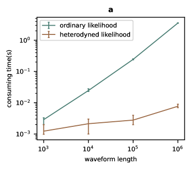
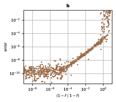
Figure 1: The left panel shows the computing time for waveforms using heterodyned likelihood and ordinary likelihood for different waveform lengths. Mean value and 90% confidence intervals are shown over 1,000 waveforms. The right panel shows how the error between heterodyned likelihood and ordinary likelihood are correlated with the deviation of the slow term $\widetilde{r}\left(f\right)$. A strong correlation between the error and the $\langle 1-\widetilde{r}|1-\widetilde{r}\rangle$ can be observed. This indicates that if $\widetilde{r}\left(f\right)$ is indeed slowly changing, then the heterodyned likelihood method can compute the likelihood accurately.

IV The Analysis Pipeline of TianQin for MBHB

For heliocentric orbit missions like LISA, the data downlink speed/cadence is limited by the availability of deep space networks. Therefore, it would be relatively challenging and expensive to afford near real-time data transmission. On the other hand, for geocentric orbit missions like TianQin, if inter-satellite communication is enabled and/or multiple ground facilities are available to ensure data downlink, it is possible to expect reliable and near real-time data downlink. Even in the pessimistic scenario that the near real-time downlink is not available all the time, a data receiving cadence of two days can be assumed [68]. In this work, we adopt the assumption of two working modes of the data downlink of TianQin, the regular mode where the full amount of data is available with a latency of two days; and the prompt mode, where data can be transferred almost real time.

The SNR accumulation of GW signals from MBHBs are highly non-linear, with the last hour signal accounting for as much as 99% of the SNR. Therefore, long before the MBHB mergers, the data transmission cadence does not imply huge differences, and we adopt the assumption that new data is available every two days. In this first stage, we apply the search module that runs every two days, to routinely check if an upcoming MBHB merger contains large enough SNR. If the SNR exceeds 8, we conclude that a signal has been detected. Otherwise, we take it as no significant MBHB signal contained in the data, and the search module will be re-run after a new batch of two-day data is received.

Once the SNR passes the threshold, we execute the module depending on the estimated merger time. The estimation module is triggered when a 90% confidence interval of merger time falls one week after the data receiving. At this time, there is still sufficient time to maintain the regular data transfer mode and perform calculations using the ordinary likelihood. When a search module or estimation module indicates that signals may merge within a week, we will crucially switch to the last stage.

Since the MBHB will merge shortly, in this last stage, we enable the real-time data transmission and also adopt the fast estimation module for the analysis. With the MBHB approaching merger, the uncertainty quickly shrinks [34]. We continuously perform the fast estimation module and update the posterior distribution result of the full parameter every hour until the merging of MBHB is estimated. Once we estimate that the MBHB have merged, the signal based on the estimated parameters will be subtracted from the data, and the search module will be re-entered to search for the next possible signal in the data without estimated signal. This cycle continues until TianQin pauses observation.

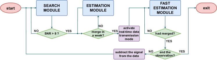
Figure 2: The flowchart of the designed pipeline. The data analysis can be separated into three modules: the search module, the estimation module, and the fast estimation module. The search module routinely searches for indications for upcoming MBHB mergers, the estimation module works if the MBHB merges after a week time, and the fast estimation module works under the assumption that real time downlink is enabled.

In Figure 2, we use the flowchart to summarize the logic of the whole pipeline. The same prior is adopted throughout all modules. For parameters that vary in orders of magnitude like $M_{c}$, a log-uniform prior is adopted. For $D_{L}$ smaller than a cutoff $D_{\rm max}=230{\rm Gpc}$ (or $z\approx 20$), we adopt a uniform prior in comoving volume, or

$$\log{p\left(D_{L}\mid I\right)}\propto 2\log{D_{L}},\quad{\rm for\ }D_{L}<D_{\rm max}$$ (13)

For other parameters, we adopt a uniform prior either for the parameter per se or over the sphere. The bounds for all parameters are shown in Table 1. Notice that since TianQin adopts “3 months on + 3 months off” working scheme, and also since most of the SNR are contributed from just before the merger, we focus on the scenario that the MBHB merges within the continuous 3 months period, so the upper limit of merger time is set to 90 days.

Table 1: The bounds for all parameters.

Parameter	Lower Bound	Upper Bound
$\log\left(M_{c}/M_{\odot}\right)$	$\log\left(10^{4}\right)$	$\log\left(10^{8}\right)$
$\eta$	$0.05$	$0.25$
$\chi_{1}$	$-1.0$	$1.0$
$\chi_{2}$	$-1.0$	$1.0$
$D_{L}/{\rm Gpc}$	$0.01$	$230$
$t_{c}/{\rm day}$	$0$	$90$
$\phi_{c}/{\rm rad}$	$0$	$2\pi$
$\psi/{\rm rad}$	$0$	$\pi$
$\cos\iota$	$-1$	$1$
$\lambda/{\rm rad}$	$0$	$2\pi$
$\sin\beta$	$-1$	$1$

For all MCMC processes, we have chosen the logarithmically uniform initial point for $M_{c}$. For sky position and $\iota$, we select initial points uniformly on the sphere. Additionally, we found that fixing the initial point of $t_{c}$ to the upper limit (3 months) enhances the sampling efficiency. As for the initial points of other parameters, we randomly select points from a uniform distribution.

IV.1 Search Module

In search module, we perform an MCMC-based analysis with 300,000 steps and 24 walkers. Note that in this stage, we evaluate likelihood with the ordinary function, and it does not significantly increase the computational burden. This is due to the fact that the frequency evolution of the binary black hole during its inspiral phase is considerably slow. One only needs to perform a calculation on limited frequency points. In practice, this module takes no more than $\sim 7$ hours on 24 CPUs Intel Xeon Silver 4210R @2.40GHz.

After the search module, the MCMC algorithm yields the maximum posterior probability and posterior distributions for all parameters. We calculate the SNR of the signal based on the parameter set associated with the maximum posterior.

IV.2 Estimation Module

The estimation module is similar to the search module, with the difference being focusing the attention on the parameter estimation. The initial points are drawn from the 90% confidence interval of the previous analysis, instead of the prior distribution as in the search module. This change can reduce the time spend on burn-in. Experiments indicate that performing an MCMC-based analysis with 24 walkers and 100,000 steps is sufficient. In practice, this module will take not more than $\sim 4$ hours, using the same hardware as the search module.

IV.3 Fast Estimation Module

When a signal is detected and estimated to merge within one week, the fast estimation module is utilized to analyze the data. The fast estimation module consists of two parts: a quick optimization using the Nelder-Mead algorithm (NM) [69], and an analysis using the heterodyned likelihood-based MCMC algorithm.

Due to the small inherent biases often present in the inferred maximum likelihood parameters, the previous analysis results may exhibit a significantly low likelihood when receiving new data. Consequently, it is not feasible to directly utilize the previous analysis results as a reference waveform for the heterodyned likelihood in the subsequent analysis. Therefore, this work utilizes the NM method in scipy.optimize to obtain a reference waveform for the heterodyned likelihood. NM method is a commonly used optimization technique. It is an iterative method that optimizes a nonlinear objective function, without requiring any gradient information. The algorithm works by defining a simplex (a set of points), and then iteratively modifying the vertices of the simplex to explore the search space and converge towards the optimal solution.

We set up NM starting from the maximum posterior estimation value in the previous analysis, with a maximum iteration of 300 to search for the parameters of maximum ordinary likelihood within the 90% confidence interval of the previous analysis. Compared to MCMC, NM is almost instantaneous, taking no more than 5 minutes. We compare the performance with other point estimation algorithms, Differential Evolution (DE) [70] and Particle Swarm Optimization (PSO) [71] in scikit-opt. In the pipeline of this work, on the one hand, these algorithms have similar computational accuracy, as they can obtain a reliable result with little deviation from the injected signal that is lower than $10^{-2}$. On the other hand, NM has a speed advantage over the other point estimation algorithms.

After obtaining the reference parameters provided by NM, we apply the heterodyned likelihood-based MCMC algorithm. Heterodyned likelihood greatly improves the calculation speed of the likelihood function under small errors, enabling us to obtain the results within $\sim 40$ minutes in practice, using MCMC with 24 walkers and 100,000 steps.

V Result

In order to test the performance of the pipeline, we perform the near real-time analysis on the simulated data with the injected signal as well as noise. For the Gaussian noise, we generate according to the one-sided PSD of TianQin [8]. In Table 2, we summarize the parameters for the three simulated events. The first event represents the ideal case for TianQin, with the second being a heavier system, and the third with a lower SNR. For all cases, binaries will merge 2 months after the starting of TianQin observation. In Figure 3, we present the characteristic strain of all three injected waveforms for the A channel. The noise amplitude $f\sqrt{S_{n}(f)}$ is drawn with a black dashed line, where $S_{n}(f)$ is the one-sided PSD.

Table 2: The parameters of three injected sources

Parameter	Source 1	Source 2	Source 3
$M_{c}/M_{\odot}$	$3\times 10^{5}$	$3\times 10^{6}$	$3\times 10^{5}$
$\eta$	$0.15$	$0.15$	$0.15$
$\chi_{1}$	$0.5$	$0.5$	$0.5$
$\chi_{2}$	$0.7$	$0.7$	$0.7$
$D_{L}/{\rm Gpc}$	$1$	$1$	$10$
$t_{c}/{\rm day}$	$60$	$60$	$60$
$\phi_{c}/{\rm rad}$	$\pi/2$	$\pi/2$	$\pi/2$
$\psi/{\rm rad}$	$\pi/4$	$\pi/4$	$\pi/4$
$\iota/{\rm rad}$	$\pi/8$	$\pi/8$	$\pi/8$
$\lambda/{\rm rad}$	$\pi$	$\pi$	$\pi$
$\beta/{\rm rad}$	$\pi/3$	$\pi/3$	$\pi/3$
${\rm SNR}$	$2686$	$2657$	$268$

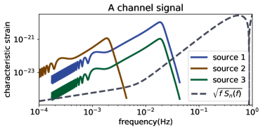
Figure 3: Each data contains a MBHB signal. The figure shows all three injected waveforms and sensitivity curves in the frequency-domain characteristic strain representation.

V.1 SNR Accumulation

The SNR of the GW signal plays a crucial role in the parameter estimation of MBHB systems. The uncertainties of many parameters say the luminosity distance, is inversely proportional to the SNR. We first provide a quantitative demonstration of the non-linear accumulation of SNR over observation time. Figure 4 shows the SNR accumulation of three different sources at different observation times. In the right panel, we also illustrate the total SNR of the complete data. One can clearly observe that the last hour of data contributes significantly to the SNR with a huge jump between lines across the panels. Both sources 1 and 2 are accompanied by relatively short distances, so they share similar total SNR. For source 1, it took 14 days to reach the SNR threshold of 8. However, the masses of source 2 are larger, and the same lower frequency cut of $10^{-4}$ Hz corresponds to a later evolution stage than source 1. Therefore, the system only enters the observation band of TianQin 6 days prior to its merger. There will only be 4 days left when it crosses the detection threshold. As for source 3, due to the relatively low SNR, it could not cross the SNR threshold of 8 until 2 days prior to the merger.

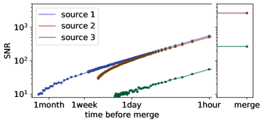
Figure 4: The SNR accumulation of three different sources at different times.

In Figure 4, we plot the evolution of SNR over time for the three sources. The horizontal axis shows the time before the merger and the vertical axis shows the SNR, and both axes are shown in logarithmic scale. For closer to the merger, the SNR grows larger and follows a power law: ${\rm SNR}\propto\left(t_{c}-t\right)^{-0.5}$. One can also observe the inclusion of Gaussian noise introduce fluctuations. On the right panel shows the final SNR that includes the contribution from the merger and the ringdown. It is evident that there’s an obvious jump between lines across the panels, indicating the significant SNR contribution of the merger and the ringdown.

V.2 Sky Localization

The main motivation for the work is to localize the massive black holes during their merger, in order to boost the chance of performing successful multi-messenger observation. Therefore, it is of vital importance to obtain accurate and prompt sky localization ability. We demonstrate the evolution of estimated sky localization uncertainties over different times for the three injected signals. To gain better intuition on the performance, some typical field of views of flagship EM telescopes were listed as a comparison.

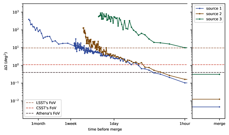
Figure 5: The time evolution of the $90\%$ confidence interval of sky localization uncertainty $\Delta\Omega$ of the three injected sources. And the fields of view of LSST ($\sim$ 9.6 deg²), CSST ($\sim$ 1.1 deg²), Athena ($\sim$ 0.4 deg²) are shown using dash line for reference.

In Figure 5, we show the time evolution of the $90\%$ confidence interval of sky localization error $\Delta\Omega$ of the three injected sources and label the FOV of three telescopes using dash line for reference. The fluctuations in the localization arise from the fluctuations in accumulation of SNR and the stochastic sample process. For comparison, we show the FOV of three representative telescopes: the Vera Rubin Telescope (LSST) [35, 36], the Chinese Space Station Telescope (CSST) [72] and the Advanced Telescope for High ENergy Astrophysics (Athena) [38]. LSST is a wide-field ground-based system with a 9.6 deg² FOV, designed to study various objects in the universe with advanced technology. CSST is a space telescope with a FOV of 1.1 deg², designed and developed by China, planned to be launched and assembled in orbit as part of the Chinese space station project. Athena is a high-energy astrophysics observatory designed by the ESA with a FOV of 0.4 deg² for studying celestial objects emitting X-rays. All these telescopes are expected to operate during TianQin’s observation period and can perform multi-messenger observations of MBHBs.

For source 1 (2), TianQin can successfully localize it within the FOV of LSST one week (2 days) prior to the merger. Since they share comparable SNRs, the localization uncertainties evolution of sources 1 and 2 are very similar one day before the final merger. In the final hours, both events can be localized in a smaller area than the FOV of CSST and then of Athena. For source 3, since it is much weaker, and is only detectable two days before the merger, the localization uncertainty is significantly larger than that of the stronger signals. The localization uncertainty only narrows down to the area comparable to the FOV of LSST in the final hour before the merger, and finally converges to nearly Athena’s FOV at the time of the merger.

If the real-time data transmission and analysis is enabled, the MBHBs can be reliably localized hours before the final merger. The localization uncertainty can be so small that a single snapshot of wide-field telescopes like the LSST could be sufficient to cover the whole interesting area, and the EM follow-up observation strategy can be significantly simplified [73]. If only the regular data transmission mode is available, one has to wait up to two days before the arrival of a new batch of data, then only the stronger sources can be localized to the level of LSST FOV. Rich information about the merger could be lost as EM telescopes can easily miss the target at the right time.

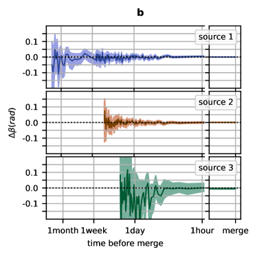
Figure 6: The evolution of the estimation error of the ecliptic longitude (left panel) and the ecliptic latitude (right panel) for the three injected sources. The shaded region represents the $90\%$ confidence interval, while the solid line represents the error of the mean value.

In Figure 6, we present the evolution of the estimation error of the ecliptic latitude and the ecliptic longitude. Compared with ecliptic longitude, ecliptic latitude can be slightly better constrained by TianQin due to its configuration. We remark that the injected value lies consistently within the 90% confidence intervals throughout the whole process, indicating that our near real-time analysis can present reliable sky localization.

V.3 Other Parameters Constraint

Finally, we discuss TianQin’s capability to constrain other parameters for the three sources, especially the luminosity distance and the merger time. The precise measurement of the luminosity distance plays a significant role in reducing the number of potential host galaxies, and the precise estimate of the merger time is of vital importance to coordinated multi-messenger observation.

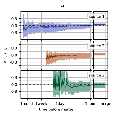
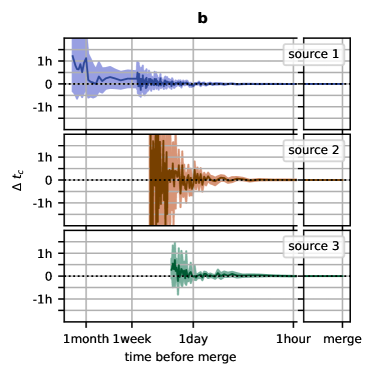
Figure 7: Similar to Figure 6, but for the relative errors of luminosity distance (left panel) and the errors of merger time in units of second (right panel).

In addition to the ecliptic longitude and ecliptic latitude, in order to localize the sources in the three dimension space, one would need to also constrain the luminosity distance of the source. Notice that a given sky area could contain multiple galaxies. If one wishes to use the GW observation of MBHBs to perform inference on the cosmological parameters, the successful identification of the host galaxy would be very important [74]. Figure 7 shows the evolution of the luminosity distance uncertainties for three sources. For the three sources, the final uncertainties for the luminosity distances are 7.9%, 8.5%, and 22.0%. Although the SNRs for the three signals are high, the degeneracy between the luminosity distance and the inclination angle prevents it from a more precise measurement. The future inclusion of higher modes [75] or a network of multiple detectors [76] can break such degeneracy.

In this study, we choose to turn on the real time data analysis when the MBHB is expected to merge in one week time. Therefore, the precise and reliable measurement of the merger time is critical to this work. In Figure 7, we present the evolution of the estimated merger time uncertainties. When the signal is first detected, the merger time estimation may have an error of about a few hours for sources 1 and 3. While for source 2, in the first few hours after the detection, the uncertainty of merger time could be over one day due to the insufficient frequency evolution. However, the merger time uncertainty of source 2 could be significantly reduced over the time scale of hours. Within one day before the merger, the uncertainty shrinks to the level of 10 minutes for source 1 and 1 hour for sources 2 and 3. If all data is used, the merger time estimation uncertainties for the three sources further shrink to 0.7 seconds, 6.6 seconds, and 23.2 seconds, respectively. In all cases, the forecast of the merger is accurate enough so that the real time data transmission will happen timely.

Table 3: The mean value and 90% confidence intervals for deviation from injected value, columns represent different sources and lines represent different parameters.

Parameter	Source 1	Source 2	Source 3
$\Delta M_{c}/M_{\odot}$	$+3.42^{+4.24}_{-4.18}$	$-26.98^{+486.08}_{-502.31}$	$+43.21^{+44.94}_{-47.11}$
$\Delta\eta$	$\left(-4.34^{+9.20}_{-9.32}\right)\times 10^{-5}$	$\left(-0.42^{+6.00}_{-6.12}\right)\times 10^{-5}$	$\left(-0.35^{+1.13}_{-1.04}\right)\times 10^{-3}$
$\Delta\chi_{1}$	$\left(+2.75^{+6.12}_{-6.14}\right)\times 10^{-4}$	$\left(-1.83^{+5.53}_{-5.87}\right)\times 10^{-4}$	$\left(-0.19^{+0.94}_{-1.30}\right)\times 10^{-2}$
$\Delta\chi_{2}$	$\left(-1.53^{+2.50}_{-2.51}\right)\times 10^{-3}$	$\left(+0.89^{+1.85}_{-1.87}\right)\times 10^{-3}$	$\left(+1.20^{+6.43}_{-4.49}\right)\times 10^{-2}$
$\Delta D_{L}/{\rm Gpc}$	$\left(+4.62^{+2.94}_{-4.98}\right)\times 10^{-2}$	$\left(+4.32^{+3.21}_{-5.28}\right)\times 10^{-2}$	$-0.14^{+0.86}_{-1.34}$
$\Delta t_{c}/{\rm s}$	$+0.20^{+0.36}_{-0.35}$	$-1.66^{+3.33}_{-3.30}$	$-3.63^{+9.40}_{-13.75}$
$\Delta\phi_{c}/{\rm rad}$	$-0.28^{+0.86}_{-1.12}$	$-0.49^{+1.10}_{-0.92}$	$-0.53^{+1.15}_{-0.91}$
$\Delta\psi/{\rm rad}$	$+0.41^{+1.06}_{-1.04}$	$+0.48^{+0.93}_{-1.10}$	$+0.30^{+1.10}_{-0.94}$
$\Delta\iota/{\rm rad}$	$-0.14^{+0.15}_{-0.16}$	$-0.13^{+0.15}_{-0.17}$	$-0.04^{+0.25}_{-0.27}$
$\Delta\lambda/{\rm rad}$	$\left(+1.92^{+9.51}_{-8.01}\right)\times 10^{-4}$	$\left(-0.64^{+1.44}_{-1.40}\right)\times 10^{-3}$	$\left(-0.78^{+8.92}_{-7.60}\right)\times 10^{-3}$
$\Delta\beta/{\rm rad}$	$\left(+3.17^{+5.84}_{-5.85}\right)\times 10^{-4}$	$\left(+6.67^{+9.83}_{-9.76}\right)\times 10^{-4}$	$\left(-3.67^{+4.28}_{-4.21}\right)\times 10^{-3}$

In Table 3, we present the estimated uncertainties of all 11 parameters for the MBHBs, using all data including the merger and ringdown phase. In terms of relative uncertainty, the redshifted chirp mass is the most precisely constrained parameter. For source 1, the chirp mass’s confidence interval is confined to about $3\times 10^{-5}$ around the true value. For sources 2 and 3, the confidence interval can also be narrowed down to about $3\times 10^{-4}$. Additionally, the merger phase and polarization angle are almost entirely unconstrained. The uncertainty for the inclination angle is also substantial, which greatly hinders the precise constraining of the luminosity distance.

VI Discussion

The multi-messenger observations of MBHBs have significant scientific implications, yet they also impose requirements on our data transmission and analysis abilities. In this work, we consider the TianQin mission and construct a quick analysis pipeline. The geocentric orbit of the TianQin mission makes it possible to enable real-time data transmission, and we consider the two working modes of data transmission: the regular and the prompt. We assume that we can enable the real-time transmission if a MBHB is believed to merge in a week’s time.

We inject three simulated signals into Gaussian noise and test the performance of our data analysis pipelines under different working modes. The results illustrate the necessity of real time transmission. Without this, accurate sky positioning for the majority of MBHBs before the merger event would prove challenging. Furthermore, we have demonstrated our real-time data analysis capabilities, which enable us to accurately constrain most of the parameters in time. For sources with higher SNR, it is possible to narrow down the localization region to within the FOV of around 1 square degree 1 hour before the merger. For sources with lower SNR, the same level of localization uncertainty can be reached with post-merger data.

As a preliminary exploration, our work suffers from potential caveats. For example, we simulate and analyse the noise under the Gaussian and stationary assumptions. In reality, these assumptions might not hold true. We might also need to update the PSD when a more realistic prediction is available. For the injected signal, the IMRPhenomD waveform model used in this work does not include higher-order modes. Future work will consider performing fast analysis with higher-order modes. Higher-order modes can break degeneracy, such as luminosity distance-inclination degeneracy, not only making the related parameters distributions could be better constrained but also improving the sampling efficiency. Finally, we ignore the impact of all other sources like the Galactic binaries, or realistic features like data gaps. We leave the inclusion and treatment of these more realistic issues for future exploration.

VII Acknowledge

We would like to thank Jian-Dong Zhang, Shuai Liu, Xue-Ting Zhang, Lu Wang and Han Wang for helpful comments. We are indebted to Xue-Feng Zhang and Zhao-Xiang Yi for constructive discussions on the data downlink of TianQin. This work has been supported by the Natural Science Foundation of China (Grants No. 12173104, No. 12261131504), and Guangdong Major Project of Basic and Applied Basic Research (Grant No. 2019B030302001).

References

- Abbott et al. [2019] B. P. Abbott, R. Abbott, T. D. Abbott, S. Abraham, F. Acernese, et al., Physical Review X 9, 031040 (2019), eprint 1811.12907.
- Abbott et al. [2021a] R. Abbott, T. D. Abbott, S. Abraham, F. Acernese, K. Ackley, et al., Physical Review X 11, 021053 (2021a), eprint 2010.14527.
- Abbott et al. [2021b] R. Abbott, T. D. Abbott, F. Acernese, K. Ackley, C. Adams, et al., arXiv e-prints arXiv:2111.03606 (2021b), eprint 2111.03606.
- Agazie et al. [2023] G. Agazie, A. Anumarlapudi, A. M. Archibald, Z. Arzoumanian, P. T. Baker, B. Bécsy, L. Blecha, A. Brazier, P. R. Brook, S. Burke-Spolaor, et al., The Astrophysical Journal Letters 951, L8 (2023), eprint 2306.16213.
- Antoniadis et al. [2023] J. Antoniadis, P. Arumugam, S. Arumugam, S. Babak, M. Bagchi, A. S. Bak Nielsen, C. G. Bassa, A. Bathula, A. Berthereau, M. Bonetti, et al., arXiv e-prints arXiv:2306.16214 (2023), eprint 2306.16214.
- Reardon et al. [2023] D. J. Reardon, A. Zic, R. M. Shannon, G. B. Hobbs, M. Bailes, V. Di Marco, A. Kapur, A. F. Rogers, E. Thrane, J. Askew, et al., The Astrophysical Journal Letters 951, L6 (2023), eprint 2306.16215.
- Xu et al. [2023] H. Xu, S. Chen, Y. Guo, J. Jiang, B. Wang, J. Xu, Z. Xue, R. Nicolas Caballero, J. Yuan, Y. Xu, et al., Research in Astronomy and Astrophysics 23, 075024 (2023), eprint 2306.16216.
- Luo et al. [2016] J. Luo, L.-S. Chen, H.-Z. Duan, Y.-G. Gong, S. Hu, J. Ji, Q. Liu, J. Mei, V. Milyukov, M. Sazhin, et al., Classical and Quantum Gravity 33, 035010 (2016), eprint 1512.02076.
- Amaro-Seoane et al. [2017] P. Amaro-Seoane, H. Audley, S. Babak, J. Baker, E. Barausse, P. Bender, E. Berti, P. Binetruy, M. Born, D. Bortoluzzi, et al., arXiv e-prints arXiv:1702.00786 (2017), eprint 1702.00786.
- Wang et al. [2019] H.-T. Wang, Z. Jiang, A. Sesana, E. Barausse, S.-J. Huang, Y.-F. Wang, W.-F. Feng, Y. Wang, Y.-M. Hu, J. Mei, et al., Physical Review D 100, 043003 (2019), eprint 1902.04423.
- Liu et al. [2020] S. Liu, Y.-M. Hu, J.-d. Zhang, and J. Mei, Physical Review D 101, 103027 (2020), eprint 2004.14242.
- Fan et al. [2020] H.-M. Fan, Y.-M. Hu, E. Barausse, A. Sesana, J.-d. Zhang, X. Zhang, T.-G. Zi, and J. Mei, Physical Review D 102, 063016 (2020), eprint 2005.08212.
- Huang et al. [2020] S.-J. Huang, Y.-M. Hu, V. Korol, P.-C. Li, Z.-C. Liang, Y. Lu, H.-T. Wang, S. Yu, and J. Mei, Physical Review D 102, 063021 (2020), eprint 2005.07889.
- Liang et al. [2022] Z.-C. Liang, Y.-M. Hu, Y. Jiang, J. Cheng, J.-d. Zhang, and J. Mei, Physical Review D 105, 022001 (2022), eprint 2107.08643.
- Madau and Rees [2001] P. Madau and M. J. Rees, The Astrophysical Journal Letters 551, L27 (2001), eprint astro-ph/0101223.
- Volonteri et al. [2008] M. Volonteri, G. Lodato, and P. Natarajan, Monthly Notices of the Royal Astronomical Society 383, 1079 (2008), eprint 0709.0529.
- Antonini et al. [2015] F. Antonini, E. Barausse, and J. Silk, The Astrophysical Journal 812, 72 (2015), eprint 1506.02050.
- Barnes and Hernquist [1992] J. E. Barnes and L. Hernquist, Annual Rev. Astron. Astrophys 30, 705 (1992).
- Di Matteo et al. [2005] T. Di Matteo, V. Springel, and L. Hernquist, Nature 433, 604 (2005), eprint astro-ph/0502199.
- Springel et al. [2005] V. Springel, T. Di Matteo, and L. Hernquist, Monthly Notices of the Royal Astronomical Society 361, 776 (2005), eprint astro-ph/0411108.
- Tang et al. [2018] Y. Tang, Z. Haiman, and A. MacFadyen, Monthly Notices of the Royal Astronomical Society 476, 2249 (2018), eprint 1801.02266.
- Paschalidis et al. [2021] V. Paschalidis, J. Bright, M. Ruiz, and R. Gold, The Astrophysical Journal Letters 910, L26 (2021), eprint 2102.06712.
- d’Ascoli et al. [2018] S. d’Ascoli, S. C. Noble, D. B. Bowen, M. Campanelli, J. H. Krolik, and V. Mewes, The Astrophysical Journal 865, 140 (2018), eprint 1806.05697.
- Armitage and Natarajan [2002] P. J. Armitage and P. Natarajan, The Astrophysical Journal 567, L9 (2002), eprint astro-ph/0201318.
- Chang et al. [2010] P. Chang, L. E. Strubbe, K. Menou, and E. Quataert, Monthly Notices of the Royal Astronomical Society 407, 2007 (2010), eprint 0906.0825.
- Merritt and Ekers [2002] D. Merritt and R. D. Ekers, Science 297, 1310 (2002), eprint astro-ph/0208001.
- Palenzuela et al. [2009] C. Palenzuela, M. Anderson, L. Lehner, S. L. Liebling, and D. Neilsen, Physical Review Letters 103, 081101 (2009), eprint 0905.1121.
- Palenzuela et al. [2010] C. Palenzuela, L. Lehner, and S. Yoshida, Physical Review D 81, 084007 (2010), eprint 0911.3889.
- Yuan et al. [2021] C. Yuan, K. Murase, B. T. Zhang, S. S. Kimura, and P. Mészáros, The Astrophysical Journal Letters 911, L15 (2021), eprint 2101.05788.
- Shields and Bonning [2008] G. A. Shields and E. W. Bonning, The Astrophysical Journal 682, 758 (2008), eprint 0802.3873.
- Merritt et al. [2009] D. Merritt, J. D. Schnittman, and S. Komossa, The Astrophysical Journal 699, 1690 (2009), eprint 0809.5046.
- Schnittman and Krolik [2008] J. D. Schnittman and J. H. Krolik, The Astrophysical Journal 684, 835 (2008), eprint 0802.3556.
- Mangiagli et al. [2022] A. Mangiagli, C. Caprini, M. Volonteri, S. Marsat, S. Vergani, N. Tamanini, and H. Inchauspé, Physical Review D 106, 103017 (2022), eprint 2207.10678.
- Mangiagli et al. [2020] A. Mangiagli, A. Klein, M. Bonetti, M. L. Katz, A. Sesana, M. Volonteri, M. Colpi, S. Marsat, and S. Babak, Physical Review D 102, 084056 (2020), eprint 2006.12513.
- Ivezić et al. [2019] Ž. Ivezić, S. M. Kahn, J. A. Tyson, B. Abel, E. Acosta, R. Allsman, D. Alonso, Y. AlSayyad, S. F. Anderson, J. Andrew, et al., The Astrophysical Journal 873, 111 (2019), eprint 0805.2366.
- LSST Science Collaboration et al. [2009] LSST Science Collaboration, P. A. Abell, J. Allison, S. F. Anderson, J. R. Andrew, J. R. P. Angel, L. Armus, D. Arnett, S. J. Asztalos, T. S. Axelrod, et al., arXiv e-prints arXiv:0912.0201 (2009), eprint 0912.0201.
- Shearer et al. [2010] A. Shearer, G. Kanbach, A. Slowikowska, C. Barbieri, T. Marsh, V. Dhillon, R. Mignani, D. Dravins, c. Gouiffes, C. MacKay, et al., in Proceedings of High Time Resolution Astrophysics - The Era of Extremely Large Telescopes (HTRA-IV). May 5 - 7 (2010), p. 54, eprint 1008.0605.
- Nandra et al. [2013] K. Nandra, D. Barret, X. Barcons, A. Fabian, J.-W. den Herder, L. Piro, M. Watson, C. Adami, J. Aird, J. M. Afonso, et al., arXiv e-prints arXiv:1306.2307 (2013), eprint 1306.2307.
- Dewdney et al. [2009] P. E. Dewdney, P. J. Hall, R. T. Schilizzi, and T. J. L. W. Lazio, IEEE Proceedings 97, 1482 (2009).
- Pringle [1991] J. E. Pringle, Monthly Notices of the Royal Astronomical Society 248, 754 (1991).
- Artymowicz and Lubow [1994] P. Artymowicz and S. H. Lubow, The Astrophysical Journal 421, 651 (1994).
- Inayoshi et al. [2020] K. Inayoshi, E. Visbal, and Z. Haiman, Annual Review of Astronomy and Astrophysics 58, 27 (2020), eprint 1911.05791.
- De Rosa et al. [2019] A. De Rosa, C. Vignali, T. Bogdanović, P. R. Capelo, M. Charisi, M. Dotti, B. Husemann, E. Lusso, L. Mayer, Z. Paragi, et al., New Astronomy Reviews 86, 101525 (2019), eprint 2001.06293.
- Schutz [1986] B. F. Schutz, Nature 323, 310 (1986).
- Tamanini et al. [2016] N. Tamanini, C. Caprini, E. Barausse, A. Sesana, A. Klein, and A. Petiteau, Journal of Cosmology and Astroparticle Physics 2016, 002 (2016), eprint 1601.07112.
- Corman et al. [2022] M. Corman, A. Ghosh, C. Escamilla-Rivera, M. A. Hendry, S. Marsat, and N. Tamanini, Physical Review D 105, 064061 (2022), eprint 2109.08748.
- Haiman [2017] Z. Haiman, Physical Review D 96, 023004 (2017), eprint 1705.06765.
- Feng et al. [2019] W.-F. Feng, H.-T. Wang, X.-C. Hu, Y.-M. Hu, and Y. Wang, Phys. Rev. D 99, 123002 (2019), eprint 1901.02159.
- Cornish [2010] N. J. Cornish, arXiv e-prints arXiv:1007.4820 (2010), eprint 1007.4820.
- Cornish [2021] N. J. Cornish, Physical Review D 104, 104054 (2021), eprint 2109.02728.
- Zackay et al. [2018] B. Zackay, L. Dai, and T. Venumadhav, arXiv e-prints arXiv:1806.08792 (2018), eprint 1806.08792.
- Canizares et al. [2013] P. Canizares, S. E. Field, J. R. Gair, and M. Tiglio, Physical Review D 87, 124005 (2013), eprint 1304.0462.
- Vinciguerra et al. [2017] S. Vinciguerra, J. Veitch, and I. Mandel, Classical and Quantum Gravity 34, 115006 (2017), eprint 1703.02062.
- Morisaki [2021] S. Morisaki, Physical Review D 104, 044062 (2021), eprint 2104.07813.
- Katz [2022] M. L. Katz, Physical Review D 105, 044055 (2022), eprint 2111.01064.
- Husa et al. [2016] S. Husa, S. Khan, M. Hannam, M. Pürrer, F. Ohme, X. J. Forteza, and A. Bohé, Physical Review D 93, 044006 (2016), eprint 1508.07250.
- Khan et al. [2016] S. Khan, S. Husa, M. Hannam, F. Ohme, M. Pürrer, X. J. Forteza, and A. Bohé, Physical Review D 93, 044007 (2016), eprint 1508.07253.
- Digman and Cornish [2022] M. C. Digman and N. J. Cornish, arXiv e-prints arXiv:2212.04600 (2022), eprint 2212.04600.
- Marsat et al. [2021] S. Marsat, J. G. Baker, and T. D. Canton, Physical Review D 103, 083011 (2021), eprint 2003.00357.
- Vallisneri [2005] M. Vallisneri, Physical Review D 71, 022001 (2005), eprint gr-qc/0407102.
- Królak et al. [2004] A. Królak, M. Tinto, and M. Vallisneri, Physical Review D 70, 022003 (2004), eprint gr-qc/0401108.
- Cornish and Hellings [2003] N. J. Cornish and R. W. Hellings, Classical and Quantum Gravity 20, 4851 (2003), eprint gr-qc/0306096.
- Shaddock et al. [2003] D. A. Shaddock, M. Tinto, F. B. Estabrook, and J. W. Armstrong, Physical Review D 68, 061303 (2003), eprint gr-qc/0307080.
- Tinto et al. [2004] M. Tinto, F. B. Estabrook, and J. W. Armstrong, Physical Review D 69, 082001 (2004), eprint gr-qc/0310017.
- Hu et al. [2018] X.-C. Hu, X.-H. Li, Y. Wang, W.-F. Feng, M.-Y. Zhou, Y.-M. Hu, S.-C. Hu, J.-W. Mei, and C.-G. Shao, Classical and Quantum Gravity 35, 095008 (2018), eprint 1803.03368.
- Foreman-Mackey et al. [2013] D. Foreman-Mackey, D. W. Hogg, D. Lang, and J. Goodman, Publications of the Astronomical Society of the Pacific 125, 306 (2013), eprint 1202.3665.
- Goodman and Weare [2010] J. Goodman and J. Weare, Communications in Applied Mathematics and Computational Science 5, 65 (2010).
- Zhang and Yi [2023] X. Zhang and Z. Yi, private communication (2023).
- Gao and Han [2012] F. Gao and L. Han, Computational Optimization and Applications 51, 259–277 (2012).
- Storn and Price [1997] R. Storn and K. Price, Journal of Global Optimization 11, 341 (1997).
- Kennedy [2010] J. Kennedy, Particle Swarm Optimization (Springer US, Boston, MA, 2010), pp. 760–766, ISBN 978-0-387-30164-8, URL https://doi.org/10.1007/978-0-387-30164-8_630.
- Gong et al. [2019] Y. Gong, X. Liu, Y. Cao, X. Chen, Z. Fan, R. Li, X.-D. Li, Z. Li, X. Zhang, and H. Zhan, The Astrophysical Journal 883, 203 (2019), eprint 1901.04634.
- Chan et al. [2017] M. L. Chan, Y.-M. Hu, C. Messenger, M. Hendry, and I. S. Heng, Astrophys. J. 834, 84 (2017), eprint 1506.04035.
- Zhu et al. [2022] L.-G. Zhu, Y.-M. Hu, H.-T. Wang, J.-d. Zhang, X.-D. Li, M. Hendry, and J. Mei, Phys. Rev. Res. 4, 013247 (2022), eprint 2104.11956.
- London et al. [2018] L. London, S. Khan, E. Fauchon-Jones, C. García, M. Hannam, S. Husa, X. Jiménez-Forteza, C. Kalaghatgi, F. Ohme, and F. Pannarale, Physical Review Letters 120, 161102 (2018), eprint 1708.00404.
- Shuman and Cornish [2022] K. J. Shuman and N. J. Cornish, Physical Review D 105, 064055 (2022), eprint 2105.02943.