Work Statistics and Adiabatic Assumption in Nonequilibrium Many-Body Theory

Abstract

Keldysh field theory, based on adiabatic assumptions, serves as an widely used framework for addressing nonequilibrium many-body systems. Nonetheless, the validity of such adiabatic assumptions when addressing interacting Gibbs states remains a topic of contention. We use the knowledge of work statistics developed in nonequilibrium thermodynamics to study this problem. Consequently, we deduce a universal theorem delineating the characteristics of evolutions that transition an initial Gibbs state to another. Based on this theorem, we analytically ascertain that adiabatic evolutions fail to transition a non-interacting Gibbs state to its interacting counterpart. However, this adiabatic approach remains a superior approximation relative to its non-adiabatic counterpart. Numerics verifying our theory and predictions are also provided. Furthermore, our findings render insights into the preparation of Gibbs states within the domain of quantum computation.

Introduction.—The concept of adiabatic driving has been widely used in quantum physics, including Berry phase Berry (1984), zero-temperature many-body theory Fetter and Walecka (2012); Coleman (2015), nonequilibrium many-body theory Keldysh (1965); Kamenev (2011); Stefanucci and Van Leeuwen (2013), and adiabatic quantum computation Albash and Lidar (2018). The adiabatic theorem Born and Fock (1928); Kato (1950); Griffiths and Schroeter (2018); Sakurai and Commins (1995) guarantees the validity of the adiabatic assumption in studying those physics. Specifically, in the zero-temperature many-body (field) theory, the Gell-Mann-Low theorem Gell-Mann and Low (1951); Fetter and Walecka (2012); Coleman (2015), which is a specialization of the adiabatic theorem for interacting many-body systems, indicates that one can obtain the interacting ground state from a non-interacting ground state by adiabatically switching on the interaction Hamiltonian. Such a reduction greatly facilitate the treatment of interacting systems, as it makes the non-interacting Green’s functions as the building blocks.

Based on the Schwinger-Keldysh closed time formalism Schwinger (1961); Keldysh (1965); Konstantinov and Perel (1960), the nonequilibrium Green’s functions serve as a useful framework for nonequilibrium many-body problems Kamenev (2011); Kamenev and Levchenko (2009); Altland and Simons (2010); Sieberer et al. (2016); Yang et al. (2021, 2023). When considering nonequilibrium many-body systems, one is often staring from a Gibbs state at inverse temperature $\beta$, where the Hamiltonian is in the form of $H=H_{0}+\lambda_{1}H_{1}$ with $H_{1}$ being the interaction Hamiltonian and $\lambda_{1}$ the interaction strength (for interacting systems, $H_{1}$ does not commute with $H_{0}$). In order to deal with such an interacting initial state, Konstantinov and Perel’ Konstantinov and Perel (1960); Stefanucci and Van Leeuwen (2013) proposed that one can regard the interacting Gibbs state as an evolution in the imaginary time axis and then treat it with the imaginary time Matsubara formalism Matsubara (1955). Despite the mathematical rigor of this approach, it presents complexities due to the concurrent handling of both imaginary-time and real-time Green’s functions. Moreover, the treatment of interacting Gibbs states using Matsubara formalism is already a difficult task. Therefore, a streamlined formalism, predominantly focusing on real-time Green’s functions for nonequilibrium many-body problems, is advantageous. To this end, Keldysh suggested an approach wherein the interacting Gibbs state is considered as the final state of an evolution that initiates from a non-interacting Gibbs state at $t=-\infty$, with interactions being adiabatically switched on Keldysh (1965); Kamenev (2011); Stefanucci and Van Leeuwen (2013). Then, the building blocks reduce to non-interacting Green’s functions and one only needs to concentrate on real times, as encountered in the zero-temperature many-body theory.

In contrast to the zero-temperature many-body theory, the validity of the adiabatic assumption within the nonequilibrium many-body framework remains an open question. Specifically, if an adiabatic evolution fails to transition a non-interacting Gibbs state to an interacting Gibbs state for a specified Hamiltonian Il‘in et al. (2021), can the adiabatic assumption still be deemed a viable approximation when juxtaposed with alternative evolution protocols? Furthermore, it is pertinent to explore the inherent characteristics of such evolution protocols capable of transitioning a non-interacting Gibbs state to its interacting counterpart. Insights from these properties might prove instrumental for Gibbs state preparation methodologies Ge et al. (2016); Chowdhury et al. (2020); Wang et al. (2021). In subsequent discussions, we will refer to these evolution protocols as non-interaction-to-interaction (NI) evolution protocols.

In this work, we generally discuss these problems based on work statistics Jarzynski (1997a, b); Crooks (1998); Jarzynski (2011); Seifert (2012); Schuster (2013); Fei and Quan (2019); Ortega et al. (2019) developed in the nonequilibrium thermodynamics community. Specifically, a universal theorem that holds for arbitrary quantum systems and determines the NI evolution protocol is derived. Generic calculations of work statistics show that the adiabatic evolution can not transition a non-interacting Gibbs state to an interacting Gibbs state. However, comparing with non-adiabatic evolution protocols, the final state of the adiabatic evolution is more close to the desired interacting Gibbs state up to an error of the order of $\mathcal{O}(\lambda_{1}^{3})$. For non-adiabatic evolutions, the error is of the order of $\mathcal{O}(\lambda_{1}^{2})$.

Work statistics and Jarzynski equality.— Before examining the desired evolution protocol’s properties, we briefly review work statistics and the Jarzynski equality Jarzynski (1997a, b); Crooks (1998); Jarzynski (2011); Seifert (2012); Schuster (2013); Fei and Quan (2019); Ortega et al. (2019); Zawadzki et al. (2023) within the context of quantum mechanical Hamiltonian systems.

Ingredients of work statistics in quantum version can be defined through two energy measurements Talkner et al. (2007); Fei and Quan (2020) as shown in Fig. 1 (a). In the first measurement, the energy outcome is determined by the initial Gibbs state $\rho(t_{i})=e^{-\beta H(t_{i})}/Z(t_{i})$ with $Z(t_{i})=\operatorname{tr}[e^{-\beta H(t_{i})}]$ being the partition function of the initial system. The first measurement can produce an eigenvalue $E_{n}^{i}$ of $H(t_{i})$ with a probability $p_{n}=e^{-\beta E_{n}^{i}}/Z(t_{i})$. Subsequent to this, the system transitions to the eigenstate $|\psi_{n}^{i}\rangle$ and evolves according to the time-dependent Hamiltonian $H(t)$ under the unitary evolution $U(t)$. At the final time $t_{f}$, another measurement results in the eigenvalue $E_{m}^{f}$ of $H(t_{f})$ with a conditional probability $p(m,t_{f}|n,t_{i})=\left|\langle\psi_{m}^{f}|U(t_{f})|\psi_{n}^{i}\rangle\right|^{2}$. Here, $|\psi_{m}^{f}\rangle$ signifies the eigenstate of $H(t_{f})$ corresponding to $E_{m}^{f}$. Consequently, the joint probability of obtaining measurements $E_{m}^{f}$ and $E_{n}^{i}$ is $p(m,t_{f}|n,t_{i})p_{n}$. The work is defined as the difference of two energy outcomes: $w=E_{m}^{f}-E_{n}^{i}$, and the probability of work $w$ should be

$$p(w)=\sum_{n,m}\delta\left[w-(E_{m}^{f}-E_{n}^{i})\right]p(m,t_{f}|n,t_{i})p_{n}.$$ (1)

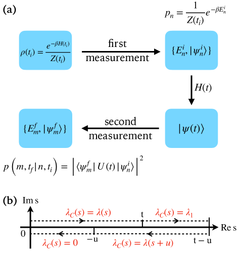
Figure 1: (a) Definition of work statistics through two energy measurements. (b) The contour $C$ used in calculating the characteristic function of work. The contour $C$ is divided into four parts for our case: $(i)$ $0\rightarrow t$: $\lambda_{C}\left(s\right)=\lambda\left(s\right)$; $(ii)$ $t\rightarrow t-u$ with $u<0$: $\lambda_{C}\left(s\right)=\lambda_{1}$; $(iii)$ $t-u\rightarrow t$: $\lambda_{C}\left(s\right)=\lambda\left(s+u\right)$; $(iv)$ $-u\rightarrow 0$: $\lambda_{C}(s)=0$.

Having derived the work distribution, one can also define the characteristic function of work (CFW) through the Fourier transformation of $p(w)$:

$$\begin{split}\chi(u)&=\int dwe^{iuw}p(w)\\ &=\frac{1}{Z(t_{i})}\operatorname{tr}\left[U^{\dagger}(t_{f})e^{iuH(t_{f})}U(t_{f})e^{-(iu+\beta)H(t_{i})}\right].\end{split}$$ (2)

The CFW is a more convenient tool in studying nonequilibrium physics of quantum systems than the distribution $p(w)$. Remarkably, by setting $u=i\beta$ in the CFW, one can obtain the Jarzynski equality Jarzynski (1997a):

$$\left\langle e^{-\beta w}\right\rangle=\frac{Z(t_{f})}{Z(t_{i})},$$ (3)

where $\langle\cdot\rangle$ without subscript is defined as $\langle\cdot\rangle=\int dw(\cdot)p(w)$, and $Z(t_{f})=\operatorname{tr}[e^{-\beta H(t_{f})}]$ is the partition function of a hypothetical system with Hamiltonian $H(t_{f})$ in a Gibbs state at inverse temperature $\beta$. Note that the real system at $t_{f}$ is not necessarily at a Gibbs state. Hence, it is also desirable to ask that when the real system will be in a Gibbs state at $t_{f}$.

Properties of the non-interaction-to-interaction (NI) evolution protocol.—In the subsequent section, we will present our central theorem elucidating the properties of the NI evolution protocol. Prior to that, we introduce two lemmas essential for the theorem’s proof. We provide only a succinct overview of the pivotal steps in the proof, with comprehensive details available in the Supplementary Information (SI) sup .

Lemma 1. The averaged work $\langle w\rangle\equiv\int dwwp\left(w\right)$ of an evolution from $t_{i}$ to $t_{f}$, can also be expressed as $\langle w\rangle=\langle H\left(t_{f}\right)\rangle_{t_{f}}-\langle H\left(t_{i}\right)\rangle_{t_{i}}$, where $\langle H\left(t\right)\rangle_{t}\equiv\operatorname{tr}\left[\rho\left(t\right)H\left(t\right)\right]$.

Lemma 2. Suppose there exists an evolution protocol from $t_{i}$ to $t_{f}$, such that for all systems, the average work of the evolution satisfies $\langle w\rangle=\langle H(t_{f})\rangle_{G}-\langle H(t_{i})\rangle_{t_{i}}$, where

$$\langle H(t_{f})\rangle_{G}\equiv\frac{1}{\operatorname{tr}\left[e^{-\beta H(t_{f})}\right]}\operatorname{tr}\left[e^{-\beta H(t_{f})}H(t_{f})\right],$$

then the final state $\rho(t_{f})$ is a Gibbs state with respect to $H(t_{f})$ at inverse temperature $\beta$.

Having derived the above two lemmas, we are now in a position to prove our central theorem, which gives the property of the desired evolution protocol for arbitrary systems.

Theorem 1. Suppose there exists an evolution protocol from $t_{i}$ to $t_{f}$, such that for all systems, the evolution will drive the initial Gibbs state $\rho(t_{i})=e^{-\beta H(t_{i})}/Z(t_{i})$ to a final state (at $t_{f}$), which is a Gibbs state with respect to $H(t_{f})$ at inverse termperature $\beta$. This evolution protocol exists if and only if the work distribution $p(w)$ is a delta function for all systems.

Proof. a). We first prove the sufficiency: If the work distribution is $p(w)=\delta(w-w_{0})$ (For different systems, $w_{0}$ can be different), then the work of each trajectory should be the same, and equals to the average $\langle w\rangle$. According to the Jarzynski equality Eq. (3), one has

$$\left\langle e^{-\beta w}\right\rangle=e^{-\beta w_{0}}=\frac{Z\left(t_{f}\right)}{Z\left(t_{i}\right)},$$ (4)

where $Z(t_{f})$ is the partition function of a hypothetical system with Hamiltonian $H(t_{f})$ in a Gibbs state at inverse temperature $\beta$. Then

$$\begin{split}w_{0}&=-\frac{\partial}{\partial\beta}\ln\frac{Z\left(t_{f}\right)}{Z\left(t_{i}\right)}\\ \Rightarrow\langle w\rangle&=-\frac{\partial}{\partial\beta}\ln\frac{Z\left(t_{f}\right)}{Z\left(t_{i}\right)}\\ &=\langle H\left(t_{f}\right)\rangle_{G}-\langle H\left(t_{i}\right)\rangle_{t_{i}}.\end{split}$$ (5)

According to Lemma 2, we know that the state of the real system at $t_{f}$ is also the Gibbs state $\rho(t_{f})=\exp{[-\beta H\left(t_{f}\right)]}/Z(t_{f})$.
b). We then prove the necessity: If the state at $t_{f}$ is $\rho(t_{f})=\exp{[-\beta H\left(t_{f}\right)]}/Z(t_{f})$, then according to Lemma 1, one has

$$\begin{split}\langle w\rangle&=\left\langle H\left(t_{f}\right)\right\rangle_{t_{f}}-\langle H\left(t_{i}\right)\rangle_{t_{i}}\\ &=-\frac{\partial}{\partial\beta}\ln\frac{Z\left(t_{f}\right)}{Z\left(t_{i}\right)}.\end{split}$$ (6)

In addition, the Jarzynski equality will lead to

$$\begin{split}-\frac{\partial}{\partial\beta}\ln\left\langle e^{-\beta w}\right\rangle&=-\frac{\partial}{\partial\beta}\ln\frac{Z\left(t_{f}\right)}{Z\left(t_{i}\right)}.\end{split}$$ (7)

Combinging Eq. (6) and Eq. (7), one has

$$\begin{split}\langle w\rangle&=-\frac{\partial}{\partial\beta}\ln\left\langle e^{-\beta w}\right\rangle\\ \Rightarrow\quad 0&=\left\langle w\left(\frac{1}{\langle e^{-\beta w}\rangle}e^{-\beta w}-1\right)\right\rangle.\end{split}$$ (8)

Since this equation holds for all systems, the outer $\langle\cdot\rangle$ operation can be dropped, that is

$$\begin{split}0&=\frac{1}{\langle e^{-\beta w}\rangle}e^{-\beta w}-1\\ \Rightarrow e^{-\beta w}&=\left\langle e^{-\beta w}\right\rangle\\ \Rightarrow\quad\;\,w&=w_{0},\end{split}$$ (9)

where $w_{0}$ is a constant but can be different for different systems. Therefore, the work distribution for the desired evolution protocol should be

$$p(w)=\delta(w-w_{0}).$$ (10)

$\hfill\boxempty$

The time-independent case is a trivial example of this theorem. In this case, the final Gibbs state is identical with the initial Gibbs state, and the state after the first measurement only acquires a overall phase under the evolution provided by the time-independent Hamiltonian. Thus the trajectory work is simply $w=w_{0}=0$.

Given the utility of the characteristic function of work (CFW) in facilitating analysis, we derive a corollary based on Theorem 1 in order to capture the property through the CFW.

Corollary 1. The logarithm of the characteristic function of work $\chi(u)$ for the evolution protocol given by Theorem 1 satisfies $\ln\chi(u)=iuw_{0}$, where $w_{0}$ is a real number.

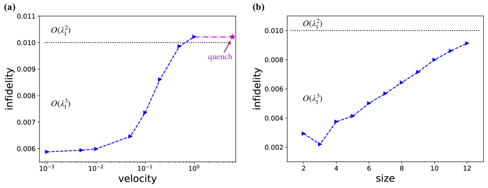
Figure 2: Infidelities ($1-$fidelity) between the interacting Gibbs state and final states of different evolution protocols. The parameters in common are chosen to be $J=2,\,\lambda_{1}=0.1,\,\beta=1$. The total time for each evolution is $\lambda_{1}/0.001=100$. (a) Infidelities for different evolution velocities of the linear driving $\lambda(t)=vt$. The size of the XXZ chain is chosen to be $N=11$. The final point marked as a star represents the quench evolution protocol, the velocity of which is regarded as $\infty$. For velocities larger than $0.001$, the system will reach the full interaction before $t=100$, and then the system will continue to evolve with full interaction until time reaches $100$. (b) Infidelities for different sizes of the XXZ chain. The increasing velocity is chosen to be $v=0.2$ and the evolution time is also $t=100$.

Perturbative calculations of the characteristic function of work.—For systems under an arbitrary nonequilibrium protocol, computing the CFW can be challenging. Nonetheless, when the full interaction strength, denoted as $\lambda_{1}$, within the Hamiltonian $H=H_{0}+\lambda_{1}H_{1}$ remains small, a universal formula for the CFW can be derived via perturbation theory Fei and Quan (2020). Given the suitability of field theory techniques to weakly interacting quantum many-body systems, our focus predominantly lies within the perturbative domain.

Given the time evolution protocol where the interaction is gradually turned on from $0$ to $t$, we recognize that the exponential operators in Eq. (2) can all be treated as evolution operators along either real-time axis or imaginary-time axis. Thus, analogous to the Schwinger-Keldysh contour formalism, the CFW can be written in a contour-integral form Fei and Quan (2020):

$$\begin{split}\chi\left(u\right)=\left\langle\mathcal{T}_{C}\left[e^{-i\int_{C}ds\lambda_{C}\left(s\right)H_{1}^{I}(s)}\right]\right\rangle_{0},\end{split}$$ (11)

where $\langle\cdot\rangle_{0}=\operatorname{tr}[(\cdot)e^{-\beta H_{0}}]/\operatorname{tr}[e^{-\beta H_{0}}]$, $\mathcal{T}_{C}$ is the contour-ordered operator with $C$ being the contour analogous to the Schwinger-Keldysh contour, and $H_{1}^{I}\left(s\right)=e^{iH_{0}s}H_{1}e^{-iH_{0}s}$ is the interacting Hamiltonian in the interaction picture. The contour is divided into four parts as shown in Fig. 1 (b), according to the value of $\lambda_{C}(s)$. As the initial interaction strength is $0$, the contour only resides on the real-time axis.

The logarithm of $\chi\left(u\right)$, known as the cumulant CFW, can be expanded through the cumulant correlation function Kubo (1962):

$$\begin{split}\ln\chi\left(u\right)=\sum_{n=1}^{\infty}\int_{C}d\bar{s}_{1}\cdots d\bar{s}_{n}G_{c}\left(s_{1},\cdots,s_{n}\right),\end{split}$$ (12)

where $d\bar{s}_{l}\equiv ds_{l}\lambda_{C}(s)\theta_{C}(s_{l}-s_{l+1})$ with $\theta_{C}(s_{l}-s_{l+1})$ being the contour step function Fei and Quan (2020) and $\theta_{C}(s_{n}-s_{n+1})\equiv 1$, and $G_{c}\left(s_{1},\cdots,s_{n}\right)\equiv\left(-i\right)^{n}\langle H_{1}^{I}\left(s_{1}\right)\cdots H_{1}^{I}\left(s_{n}\right)\rangle_{c}$ is the $n$-point cumulant correlation function.

For non-adiabatic evolutions in our case, $\ln\chi(u)$ up to second order of $\lambda_{1}$ is given by:

$$\begin{split}\ln\chi\left(u\right)=&iu\lambda_{1}\langle H_{1}\rangle_{c}+iu\lambda_{1}^{2}\int_{-\infty}^{\infty}\frac{d\omega}{2\pi}\frac{G^{>}_{c}(\omega)}{\omega}\\ &+\int_{-\infty}^{\infty}\frac{d\omega}{2\pi}\frac{1-e^{i\omega u}}{\omega^{2}}A(\omega)G^{>}_{c}(\omega)+\mathcal{O}(\lambda_{1}^{3}),\end{split}$$ (13)

where $G^{>}_{c}(\omega)$ is the Fourier transformation of $G^{>}_{c}(s_{1}-s_{2})\equiv G_{c}(s_{1},s_{2})$, and $A(\omega)\equiv|\int_{0}^{t}ds\dot{\lambda}(s)e^{i\omega s}|^{2}$. Since $G_{c}^{>}(\omega)$ is a real function, the first and second term match Corollary 1, while the third term does not. For the adiabatic case, $t\rightarrow\infty$ and $\dot{\lambda}(s)\rightarrow 0$, then the third term containing $A(\omega)$ approaches to $0$. Thus, for adiabatic cases, $\ln\chi(u)$ is linear in $u$ when we keep terms up to $\mathcal{O}(\lambda_{1}^{2})$, and then matches our theorem (or corollary). To see whether this holds for arbitrary order, we calculate $\ln\chi(u)$ up to $\mathcal{O}(\lambda_{1}^{3})$ for the adiabatic case, and obtain

$$\ln\chi\left(u\right)= iu\lambda_{1}\langle H_{1}\rangle_{c}+iu\lambda_{1}^{2}\int_{-\infty}^{\infty}\frac{d\omega}{2\pi}\frac{G_{c}^{>}(\omega)}{\omega}$$ (14)

$$+iu\lambda_{1}^{3}\int_{-\infty}^{\infty}\frac{d\omega_{1}}{2\pi}\frac{d\omega_{2}}{2\pi}\frac{G_{c}^{>}(\omega_{1},\omega_{2})}{i\omega_{1}(\omega_{1}+\omega_{2})}+\mathcal{O}(\lambda_{1}^{4}).$$

where $G_{c}^{>}(\omega_{1},\omega_{2})$ is the Fourier transformation of $G^{>}_{c}(s_{1}-s_{3},s_{2}-s_{3})$, which is defined as

$$\begin{split}&\quad G_{c}^{>}(s_{1}-s_{3},s_{2}-s_{3})\\ &\equiv(-i)^{3}\langle H_{1}^{I}(s_{1}-s_{3})H_{1}^{I}(s_{2}-s_{3})H_{1}^{I}(0)\rangle_{c}\\ &=G_{c}(s_{1},s_{2},s_{3})\end{split}$$ (15)

Notice that $\mathcal{O}(\lambda_{1}^{3})$ term does not match Corollary 1, as one can demonstrate that $G_{c}^{>}(\omega_{1},\omega_{2})$ is a complex function. Complete calculations can be found in SI sup .

Upon examining the universal criteria set by Theorem 1 (Corollary 1), we discern that neither adiabatic nor non-adiabatic evolution protocols can transition a non-interacting Gibbs state to its interacting counterpart. Notably, the logarithmic CFW for adiabatic protocols diverges from that of the NI protocol (shown in Corollary 1) to the order of $\mathcal{O}(\lambda_{1}^{3})$, while for non-adiabatic protocols, the discrepancy occurs to the order of $\mathcal{O}(\lambda_{1}^{2})$ (evident from the third term in Eq.(13)). This suggests that although adiabatic evolution doesn’t precisely achieve the desired state transition, it offers a superior approximation relative to non-adiabatic alternatives.

Numerical verification.—To verify our theory and predictions, we consider numerical results for a specific model—one-dimensional XXZ spin chain. The Hamiltonian reads

$$H_{xxz}=J\sum_{i=1}^{N-1}\left[\sigma^{+}_{i}\sigma^{-}_{i+1}+\sigma^{-}_{i+1}\sigma^{+}_{i}+\lambda(t)\sigma^{z}_{i}\sigma^{z}_{i+1}\right],$$ (16)

where $\lambda(t)$ controls the $zz$ interaction strength. For a given model, to check whether these two states are identical, one can directly compute the fidelity between the interacting Gibbs state and the final state after an evolution. Without loss of generality, we consider a linear driving protocol $\lambda(t)=vt$, where $v$ is the increasing velocity of the interaction strength. For a given system size, an evolution with larger $v$ is more non-adiabatic. We consider the small interaction regime, in which our perturbative calculation works. We finally arrive at Fig. 2 (a). One finds that larger velocities will lead to a final state more deviated from the target interacting Gibbs state. This confirms the result of our universal analysis based on work statistics. Remarkably, in the nearly adiabatic regime (small $v$), the infidelity is approximately the order of $\mathcal{O}(\lambda_{1}^{3})$, while in the non-adiabatic regime (large $v$), the infidelity is the order of $\mathcal{O}(\lambda_{1}^{2})$. This result matches the prediction based on the logarithmic CFW. For smaller sizes with identical $J$ and $\lambda_{1}$, energy gaps will be larger, thus for a fixed increasing velocity, the evolution will be more adiabatic and one is expected to see smaller infidelities. This argument is confirmed by Fig. 2 (b). In addition, the infidelity in the adiabatic regime is still the order of $\mathcal{O}(\lambda_{1}^{3})$.

Conclusion.—In summary, based on work statistics, we established a theorem elucidating the thermodynamic properties of an evolution transitioning an initial Gibbs state to another Gibbs state. In the realm of weak interactions, where the Keldysh field theory becomes particularly applicable, our theorem analytically demonstrates that adiabatic evolution does not precisely transition a non-interacting Gibbs state to its interacting counterpart. Nevertheless, when contrasted with non-adiabatic protocols, the resultant state from adiabatic evolution presents a closer approximation to the desired interacting Gibbs state. Our numerical simulation confirms the theoretical predictions.

Y. Zuo and Q. Yang contribute equally to this work.

See pages 1 of WSAA_SI.pdf See pages 2 of WSAA_SI.pdf See pages 3 of WSAA_SI.pdf See pages 4 of WSAA_SI.pdf See pages 5 of WSAA_SI.pdf See pages 6 of WSAA_SI.pdf See pages 7 of WSAA_SI.pdf

References

- Berry (1984) M. V. Berry, Proceedings of the Royal Society of London. A. Mathematical and Physical Sciences 392, 45 (1984).
- Fetter and Walecka (2012) A. L. Fetter and J. D. Walecka, Quantum theory of many-particle systems (Courier Corporation, 2012).
- Coleman (2015) P. Coleman, Introduction to Many-Body Physics (Cambridge University Press, 2015).
- Keldysh (1965) L. V. Keldysh, Sov. Phys. JETP 20, 1018 (1965).
- Kamenev (2011) A. Kamenev, Field Theory of Non-Equilibrium Systems (Cambridge University Press, 2011).
- Stefanucci and Van Leeuwen (2013) G. Stefanucci and R. Van Leeuwen, Nonequilibrium many-body theory of quantum systems: a modern introduction (Cambridge University Press, 2013).
- Albash and Lidar (2018) T. Albash and D. A. Lidar, Rev. Mod. Phys. 90, 015002 (2018).
- Born and Fock (1928) M. Born and V. Fock, Zeitschrift für Physik 51, 165 (1928).
- Kato (1950) T. Kato, Journal of the Physical Society of Japan 5, 435 (1950).
- Griffiths and Schroeter (2018) D. J. Griffiths and D. F. Schroeter, Introduction to quantum mechanics (Cambridge university press, 2018).
- Sakurai and Commins (1995) J. J. Sakurai and E. D. Commins, “Modern quantum mechanics, revised edition,” (1995).
- Gell-Mann and Low (1951) M. Gell-Mann and F. Low, Phys. Rev. 84, 350 (1951).
- Schwinger (1961) J. Schwinger, Journal of Mathematical Physics 2, 407 (1961).
- Konstantinov and Perel (1960) O. Konstantinov and V. Perel, Zhur. Eksptl’. i Teoret. Fiz. 39 (1960).
- Kamenev and Levchenko (2009) A. Kamenev and A. Levchenko, Advances in Physics 58, 197 (2009).
- Altland and Simons (2010) A. Altland and B. D. Simons, Condensed Matter Field Theory, 2nd ed. (Cambridge University Press, 2010).
- Sieberer et al. (2016) L. M. Sieberer, M. Buchhold, and S. Diehl, Reports on Progress in Physics 79, 096001 (2016).
- Yang et al. (2021) Q. Yang, Z. Yang, and D. E. Liu, Phys. Rev. B 104, 014512 (2021).
- Yang et al. (2023) Q. Yang, Y. Zuo, and D. E. Liu, Phys. Rev. Res. 5, 033174 (2023).
- Matsubara (1955) T. Matsubara, Progress of theoretical physics 14, 351 (1955).
- Il‘in et al. (2021) N. Il‘in, A. Aristova, and O. Lychkovskiy, Physical Review A 104, L030202 (2021).
- Ge et al. (2016) Y. Ge, A. Molnár, and J. I. Cirac, Phys. Rev. Lett. 116, 080503 (2016).
- Chowdhury et al. (2020) A. N. Chowdhury, G. H. Low, and N. Wiebe, (2020), arXiv:2002.00055 [quant-ph] .
- Wang et al. (2021) Y. Wang, G. Li, and X. Wang, Phys. Rev. Appl. 16, 054035 (2021).
- Jarzynski (1997a) C. Jarzynski, Phys. Rev. Lett. 78, 2690 (1997a).
- Jarzynski (1997b) C. Jarzynski, Phys. Rev. E 56, 5018 (1997b).
- Crooks (1998) G. E. Crooks, Journal of Statistical Physics 90, 1481 (1998).
- Jarzynski (2011) C. Jarzynski, Annual Review of Condensed Matter Physics 2, 329 (2011).
- Seifert (2012) U. Seifert, Reports on Progress in Physics 75, 126001 (2012).
- Schuster (2013) H. G. Schuster, Nonequilibrium statistical physics of small systems: Fluctuation relations and beyond (John Wiley & Sons, 2013).
- Fei and Quan (2019) Z. Fei and H. T. Quan, Phys. Rev. Res. 1, 033175 (2019).
- Ortega et al. (2019) A. Ortega, E. McKay, A. M. Alhambra, and E. Martín-Martínez, Phys. Rev. Lett. 122, 240604 (2019).
- Zawadzki et al. (2023) K. Zawadzki, A. Kiely, G. T. Landi, and S. Campbell, Phys. Rev. A 107, 012209 (2023).
- Talkner et al. (2007) P. Talkner, E. Lutz, and P. Hänggi, Phys. Rev. E 75, 050102 (2007).
- Fei and Quan (2020) Z. Fei and H. T. Quan, Phys. Rev. Lett. 124, 240603 (2020).
- (36) See Supplemental Information for more details.
- Kubo (1962) R. Kubo, Journal of the Physical Society of Japan 17, 1100 (1962).