The problem of dust attenuation in photometric decomposition of edge-on galaxies and possible solutions

Abstract

The presence of dust in spiral galaxies affects the ability of photometric decompositions to retrieve the parameters of their main structural components. For galaxies in an edge-on orientation, the optical depth integrated over the line-of-sight is significantly higher than for those with intermediate or face-on inclinations, so it is only natural to expect that for edge-on galaxies, dust attenuation should severely influence measured structural parameters. In this paper, we use radiative transfer simulations to generate a set of synthetic images of edge-on galaxies which are then analysed via decomposition. Our results demonstrate that for edge-on galaxies, the observed systematic errors of the fit parameters are significantly higher than for moderately inclined galaxies. Even for models with a relatively low dust content, all structural parameters suffer offsets that are far from negligible. In our search for ways to reduce the impact of dust on retrieved structural parameters, we test several approaches, including various masking methods and an analytical model that incorporates dust absorption. We show that using such techniques greatly improves the reliability of decompositions for edge-on galaxies.

1 Introduction

Measuring the physical properties of galaxies is one of the cornerstones of extragalactic astrophysics, because all theories of galaxy formation and evolution should be supported by observational data. Disc galaxies which are visible in an edge-on orientation (i.e. inclined at $i\approx 90\degr$) are of special interest in this regard because they are the only targets that facilitate a direct study of the vertical structures of disc galaxies. For example, the vertical distributions of stars, gas, and dust, as well as the possible presence of different sub-components (such as thin and thick discs), which properties are often described via various galaxy scaling relations (such as the dependence of the disc flattening on the relative mass of a spherical component, including a dark matter halo) can only be explored in edge-on galaxies (see e.g. Kylafis & Bahcall, 1987; Xilouris et al., 1999; Mosenkov et al., 2010; Bizyaev et al., 2014; Comerón et al., 2018; Mosenkov et al., 2022a).

This utility of edge-on galaxies is easily recognized due to the existence of special catalogues which were created specifically for studying the three-dimensional structure of disc galaxies. For example, the RFGC catalogue (Karachentsev et al., 1999) contains 4236 thin edge-on spiral galaxies over the whole sky. The EGIS catalog (Bizyaev et al., 2014) provides structural parameters of stellar discs (the disc scale length and scale height, as wells as the disc central surface brightness) for almost 6000 galaxies using the Sloan Digital Sky Survey (SDSS, York et al. 2000) observations in several optical wavebands. The EGIPS catalogue (Makarov et al., 2022) contains 16551 edge-on galaxies from the Pan-STARRS survey (Chambers et al., 2016; Flewelling et al., 2020).

The most widely used approach to acquire the structural parameters of galaxies is performing a photometric decomposition of their images. The main idea behind this process is to adopt an analytical model to describe the observed surface brightness distribution in a galaxy image and find the optimal parameters for such a model that yield the fewest discrepancies with the real image. There exist a number of software packages (see Peng et al. 2002; Vika et al. 2013; De Geyter et al. 2013; Erwin 2015) which were specifically designed to perform photometric decompositions of galaxies (e.g. Gadotti 2009; Lackner & Gunn 2012; Bottrell et al. 2019, and many others). For example, in almost two thousand refereed publications to date, the GALFIT code has been used to retrieve the structural parameters of galaxies with various morphologies, at different wavelengths, and in a wide range of redshifts.

Although at a first glance the main idea behind the decomposition process looks rather straightforward, there are various obstacles that must be overcome on the way to a solid and robust estimation of galaxy parameters. For example, even the model selection can be a problem, especially when working with a large sample of objects (Lingard et al., 2020). Another complicating factor is image smearing caused by a point spread function (PSF) due to atmospheric turbulence (seeing) and the physical diffraction limit. The general rule is that the smaller the galaxy component, the larger the influence of the PSF on the retrieved structural parameters (Trujillo et al., 2001a, b; Gadotti, 2009), and this is especially true for edge-on galaxies (Sandin, 2014, 2015).

In this article, we focus on another important issue for galaxy photometric decompositions that manifests particularly strongly for edge-on galaxies, dust attenuation. The dust distributed in a galaxy absorbs, scatters, and re-emits its stellar light, resulting in an observed surface brightness distribution for a galaxy image, coupled with a mass-to-stellar luminosity ratio as a function of both radius and wavelength, that does not reflect the actual mass surface density distribution over the galaxy body. This suggests that the measured structural parameters can be affected in a manner that is challenging to predict.

One possible solution to this problem is to perform radiative transfer modelling that includes the interaction between the photons and dust. The complexity of such approaches have grown over time. For example, Disney et al. (1989) provided an analysis of several simple geometric models including a “slab” model where the galaxy is considered to be a flat disc with a uniform mixture of stars, dust, and gas; a “screen” model with a stellar disc covered by a dust absorbing screen lying above the stars; and a “sandwich” model where a thin uniform dust disc is located inside of a relatively thicker stellar disc. Byun et al. (1994) performed numerical radiative transfer modelling of a three-dimensional galaxy model with various dust contents visible at different viewing angles to study how dust attenuation changes the main observables of the galaxy (ellipticity, surface brightness, exponential scale, etc.). The dust’s impact on attenuation in a galaxy as a function of wavelength was studied by Ferrara et al. (1999) for a set of different galaxy models (mimicking spiral and elliptical galaxies) and by Tuffs et al. (2004) who considered exponential discs and de Vaucouleurs bulges as separate components. A combined bulge+disc model was studied in Pierini et al. (2004).

Nowadays, there are various tools that allow one to carry out radiative transfer modeling for complex multicomponent galaxies with dust. For example, Popescu et al. (2000) describe such an approach and its application to an edge-on galaxy NGC 891. Other examples of radiative transfer programs include the TRADING code (Bianchi, 2008), the DART-RAY code (Natale et al., 2014; Natale et al., 2017), and the FITSKIRT software (De Geyter et al., 2013). For example, using FITSKIRT, it is possible to fit a galaxy image with a predefined model consisting of multiple stellar and dust components. A significant drawback of such an approach is its extreme computational cost (Mosenkov et al., 2018), and, thus, it is only useful when trying to model individual edge-on galaxies (Xilouris et al., 1997, 1998; Popescu et al., 2000; Baes et al., 2010; Bianchi & Xilouris, 2011; De Looze et al., 2012; Schechtman-Rook et al., 2012; De Geyter et al., 2013; Mosenkov et al., 2016) or small samples of galaxies (Xilouris et al., 1999; Bianchi, 2007; De Geyter et al., 2014; Mosenkov et al., 2018; Natale et al., 2022).

Another approach frequently used to investigate the effect opacity has on measured structural parameters in disc galaxies is to use radiative transfer simulations to create a mock galaxy image. This involves using a given, a-priori known model and then decomposing the image. In this case, one can explore how exactly the presence of dust affects the galactic parameters measured by using a regular decomposition technique, that is, without including the radiative transfer or any other dust compensation method. This was done by Gadotti et al. (2010), who investigated the behaviour of a couple of models of disc galaxies for a range of dust optical depth values and for inclination angles ranging from 15 to 60 degrees. A similar approach was adopted by Pastrav et al. (2013a) and Pastrav et al. (2013b) where a set of corrections for the measured decomposition parameters were computed. These corrections were applied in Pastrav (2020) to find the intrinsic (i.e. dust-corrected) parameters for several real galaxies.

In this paper, we concentrate on the effects of dust attenuation on the parameters of edge-on galaxies measured via a standard decomposition analysis. By building our article on the work done by the aforementioned studies, we opt to go further in this analysis and add some new features, such as

• using three-dimensional decomposition models with line-of-sight integration instead of traditional two-dimensional fitting, which will allow us to treat the structure of edge-on galaxies to the fullest;

• simulating real observations by accounting for instrument PSFs, transmission curves, and noise parameters;

• running simulations for a set of models to explore how mid-plane dust lanes impact galaxy structural parameters.

The other important goal of this study is to investigate various techniques to compensate for the presence of dust during the decomposition process (aside from the time-consuming radiative transfer approach). Is it possible to modify the decomposition procedure to make the derived parameters more reliable without a significant increase to computational time? If so, can we apply this approach to a large sample of edge-on galaxies? The answers to these questions are of high importance for the ongoing work with the EGIPS catalogue (Makarov et al., 2022) where we aim to perform a mass decomposition of edge-on galaxies with three-dimensional models using “dust contaminated” optical observations.

The rest of the article is organized as follows. In Section 2, we describe our algorithms for synthetic image creation and decomposition with and without correcting for dust. In Section 3, we demonstrate the results of our simulations including the dust impact on the derived decomposition parameters, and the results of applying different techniques to compensating for the presence of the dust. In Section 4, we employ the decomposition methods for retrieving the structural parameters for a couple of real galaxies, with taking a dust component into account. We state our conclusions in Section 5. Appendix A contains some technical details about the training of the neural network used throughout the paper.

2 The algorithm

In this section, we describe in detail our algorithms to investigate the dust impact on the decomposition results and propose several ways to ease these dust effects. The overall pipeline looks as follows. For a set of input parameters we create a three-dimensional model of a galaxy, and transform it into a FITS-file by projecting it on an image plane. To mimic real observations, we include a smearing effect by a PSF and add read and photon noise. We then run a standard decomposition technique to obtain the observed structural parameters of a galaxy in order to compare them with the input ones. After that, we run a series of fits using various methods, by accounting for the dust presence and without accounting for it, to see how these can amend the observed parameters.

2.1 Model functions and their parameters

In this work we consider a three-component model of a galaxy with a stellar disc, bulge, and a dust disc. As a disc model, we adopt a three-dimensional isothermal disc that follows an exponential luminosity density profile in the radial direction and a $\operatorname{sech}^{2}$ law perpendicular to the galaxy plane (van der Kruit & Searle, 1981):

$$\rho_{\mathrm{disc}}(r,z)=\rho_{0,\mathrm{disc}}\exp\left(-\frac{r}{h_{\mathrm{disc}}}\right)\operatorname{sech}^{2}\left(\frac{z}{z_{\mathrm{disc}}}\right).$$ (1)

The disc model has two geometric parameters: its radial exponential scale $h_{\mathrm{disc}}$ and the vertical scale $z_{\mathrm{disc}}$. The third parameter is the central luminosity density $\rho_{0,\mathrm{disc}}$, which governs the luminosity of the disc, but for our purposes it is more convenient to work directly with the disc’s total luminosity:

$$L_{\mathrm{disc}}=4\pi\rho_{0,\mathrm{disc}}h_{\mathrm{disc}}^{2}z_{\mathrm{disc}}.$$ (2)

Even though real galaxies can demonstrate more complex disc structures (such as the existence of two embedded stellar discs), we do not include such complexity in our simulations, because it can only be studied for the closest galaxies with better spatial resolution, and most decomposition studies utilise a single disc model.

To model a central component, we use the well-known Sérsic function (Sérsic, 1963; Sersic, 1968) that is often used to describe galactic bulges, and which have the following projected surface brightness profile:

$$I(r)=I_{0}\exp\left[-\nu_{n}\left(\frac{r}{r_{e}}\right)^{\frac{1}{n}}\right].$$ (3)

The corresponding three-dimensional density distribution that is required for our work can be found through an Abel inversion:

$$\rho_{\mathrm{bulge}}(r)=-\frac{1}{\pi}\int_{r}^{+\infty}\frac{dI}{dR}\frac{dR}{\sqrt{R^{2}-r^{2}}}.$$ (4)

In the literature there are various approaches on how to solve this integral analytically (with special functions) or numerically (Prugniel & Simien, 1997; Lima Neto et al., 1999; Baes & Gentile, 2011; Baes & van Hese, 2011; Vitral & Mamon, 2020). The bulge has three main geometric parameters (the value $\nu_{n}$ in (3) is a normalisation constant): its effective radius $r_{e}$, a Sérsic parameter $n$, and a bulge oblateness $q_{\mathrm{bulge}}$, and a parameter, that governs the overall bulge brightness, the central luminosity density $\rho_{0,\mathrm{bulge}}$, but as before, it is more convenient to use the total luminosity as a free parameter:

$$L_{\mathrm{bulge}}=\rho_{0,\mathrm{bulge}}r_{e}^{3}$$ (5)

We describe the dust component with the same isothermal disc model as the stellar disc (1) and it has the following set of geometric parameters: $h_{\mathrm{dust}}$ and $z_{\mathrm{dust}}$. Following the previous works of Gadotti et al. (2010); Pastrav et al. (2013b), we parameterize the dust content not by its central density $\rho_{0,\mathrm{dust}}$, but by using the central face-on optical depth $\tau$, that is, an integral characteristic of the galaxy opacity which can be computed by a line-of-sight integral drawn through the center of a face-on oriented model (1):

$$\tau=\int_{-\infty}^{\infty}\kappa\rho_{\mathrm{dust}}(0,z)\,dz=2\kappa z_{\mathrm{dust}}\cdot\rho_{0,dust},$$ (6)

where $\kappa$ is the extinction coefficient that depends on the dust mixture and the observed wavelength. Throughout this paper, we measure $\tau$ values in the $V$ band to be consistent with Gadotti et al. (2010), although different normalizations are used in the literature (for example, the $B$ band in Pastrav et al. 2013a, b).

The galaxy as a whole has the following free parameters (apart from parameters specific for separate components): the total bolometric luminosity $L_{\mathrm{total}}$, the bulge-to-total luminosity ratio $B/T$ (these two parameters defy the actual values of $L_{\mathrm{disc}}$ and $L_{\mathrm{bulge}}$), the luminosity distance $D_{\mathrm{L}}$, and the inclination $i$.

Theoretically, a change in any parameter in a galaxy model can lead to changes in random and systematic errors in any other parameters, but it is difficult to make a set of models that cover this parameter space well enough to study any possible inter-combinations between all parameters. To achieve the goal of this study, we settle upon the following strategy to create the model grid. We start with a single model which has the parameters of a typical disc galaxy (see, for example Gadotti 2009), listed in Tab. 1. Apart from the described set of geometric parameters above, this list also contains ages of stellar populations for the bulge and the disc such that the disc contains a younger stellar population than the bulge (4 Gyr versus 11 Gyr of a bulge), a galactic average metallicity, and a dust mixture that has mean properties found in Zubko et al. (2004). Hereafter, we will call this model a basic model. Then, we variate some parameters of this model leaving others fixed to see how these variations affect the decomposition results.

Parameter	Value
Bulge effective radius, $r_{e}$	900 pc
Bulge Sérsic index, $n$	4
Bulge oblateness, $q$	0.0
Bulge stellar population age	11 Gyr
Disc radial scalelength, $h_{\mathrm{disc}}$	4000 pc
Disc vertical scalelength, $z_{\mathrm{disc}}$	400 pc
Disc stellar population age	4 Gyr
Dust radial scalelength, $h_{\mathrm{dust}}$	4000 pc
Dust vertical scalelength, $z_{\mathrm{dust}}$	150 pc
Dust mixture	Zubko et al. (2004)
Galaxy bolometric luminosity, $L_{\mathrm{tot}}$	$10^{11}L_{\odot}$
Galaxy average metallicity	0.02
Bulge-to-total luminosity ratio, $B/T$	0.2

Table 1: The basic model parameters

2.2 Synthetic images

Creating a galaxy model with a dust component requires accurate Monte-Carlo radiative transfer simulations. For this purpose, we use the state-of-art radiative transfer code SKIRT (Baes et al., 2011; Camps & Baes, 2015, 2020). SKIRT allows one to generate panchromatic simulations of a galaxy with provided parameters for the specified structural components (in our case, these are a bulge, disc, and dust). The output data cube (a collection of two-dimensional images) contains different layers with snapshots of the galaxy model for the chosen set of wavelengths.

Next, each synthesized galaxy image from the data cube can be transformed into a new mock image to simulate observational effects which are always present in real observations. Here, we take into account specific instrument transmission curves by multiplying all $N$ individual layers of the model data cube $I_{j}(x,y)$ by the instrument response for the corresponding wavelength $f_{j}$. Then we coadd the layers into a single image $I(x,y)$, making sure to take into account the wavelength width of each layer $W_{j}$:

$$I(x,y)=\sum_{j=1}^{N}I_{j}(x,y)f_{j}W_{j}.$$ (7)

After that, it is necessary to convolve the obtained image with a PSF to simulate the effects of atmospheric and telescopic blurring. Finally, we add Gaussian and Poisson noise to the image.

For this study we decided to use the SDSS $r$ waveband as the instrument system because this survey is widely used as a data source for galaxy decompositions. Since this is an optical survey, dust attenuation can be high for edge-on galaxies. Therefore, we generate our mock galaxy images using the instrument and PSF parameters (filter transmission curve, full width at half maximum (FWHM) of PSF, gain, and readnoise values) specific for the SDSS $r$-band instrument. The average values of these characteristics (gain value equal to 4.75 electrons per count and dark variance equal to 1.32 electrons) are taken from the SDSS website. An example of a model with a face-on optical depth $\tau=1.0$ is shown on the top panel of Fig. 1.

2.3 Regular decomposition

When a mock galaxy image is ready, we use the IMFIT code (Erwin, 2015) to perform our decomposition of the image. One of the standard functions in IMFIT is a three-dimensional model of the disc which allows one to account for the projection effects and fit the galaxy inclination. Employing this function, we can reliably investigate the vertical structure of a highly inclined disc galaxy, whereas two-dimensional models of an edge-on disc work, strictly speaking, for perfect edge-on orientations only.

The IMFIT package allows one to take the PSF into account during fitting. We provide the same PSF image that we used to blur the mock image in Sec. 2.2.

The IMFIT list of models includes both a Sérsic function and a three-dimensional isothermal disc, so the output results can be directly compared with the input parameters from the SKIRT model. The only necessary step is to convert the output geometrical parameters of the IMFIT, which are given in pixels, back to parsecs using the model distance.

We emphasize that the model of the disc component that is used for the decomposition has an actual three-dimensional volume brightness distribution. To produce a projected two-dimensional model image, IMFIT performs integration along the line-of-sight $s$ of the volume luminosity density for each pixel $(x,y)$ of the image:

$$I(x,y)=\int_{-\infty}^{+\infty}\rho(s)\,\mathrm{d}s.$$ (8)

This approach requires considerably more computational time than directly computing the two-dimensional exponential surface brightness distribution. However, the advantage of this method is that it can give accurate results for models in an orientation close to edge-on. The insufficiency of a simple two-dimensional model to describe an actual three-dimensional disc is clearly shown in Pastrav et al. (2013b) where their decomposition results diverge quickly near the edge-on orientation. In Gadotti et al. (2010), the highest inclination considered was 60°which allowed them to elude this problem.

2.4 Decomposition with a dust correction

As we will see in Sec. 3, the effects of a dust component on the derived parameters of edge-on galaxies are enormous, so in some cases these make the fit results completely unreliable. To mitigate this problem, we try a number of modifications on the regular decomposition technique. In this study, we test two approaches: (i) We use different masks for the dust lane to exclude “dusty” pixels from our decomposition and (ii) we modify the decomposition model to account for the dust attenuation. Below we describe these two methods in detail.

2.4.1 Masking

The vertical scale height of the dust component in galaxies is smaller than that of the stellar disc. As a result, dust attenuation in edge-on galaxies appears as a dark narrow lane along the mid-plane of the galactic disc, whereas below and above this lane the galaxy appears less obscured. During decomposition, the analytical model fits both attenuated and unattenuated regions of the galaxy which results in systematic errors on the model’s parameters. It therefore seems promising that, by masking out the attenuated dust lane in the galaxy image, the fitting procedure can create a better model which better restores the actual galaxy parameters by only using unmasked dust-free regions of the galaxy.

The exact area to mask off is not easy to determine. A more extensive mask should better cover the regions of a galaxy affected by dust and should lead to less biased fits. On the other hand, a larger mask means less of the galaxy is actually used for fitting. In addition to that, the outer regions of galaxies are faint and have lower signal-to-noise ratios when compared to the inner galaxy regions. Thus, redundant masking is expected to make a fit less reliable. Moreover, the outermost regions of a galaxy can be dominated by other structural components, such as thick discs and halos. Therefore, masking the central galaxy region can switch the fitting, for example, from a thin disc to a thick disc and completely change the fitting results. To ascertain if there is some trade-off between our intention to better cover dust attenuated regions and, at the same time, to use as much of the galaxy data as possible, we use several different masking strategies and compare their effects on the ability to recover the true parameters of galaxies.

The simplest approach is to mask a narrow strip of a fixed height along the galaxy mid-plane. This mask has only one parameter, its height $h_{\mathrm{mask}}$ that can be varied to govern the fraction of the galaxy area to be masked. In order to link the height of the mask to the internal model parameters, we decided to measure the height in units of the dust component vertical scale $z_{\mathrm{dust}}$. Hereafter, we refer to this simple mask as the “flat” mask. An application of such a flat mask to a model image is demonstrated in the middke panel of Fig. 1 for $h_{\mathrm{mask}}$ values of 2, 4, and 6.

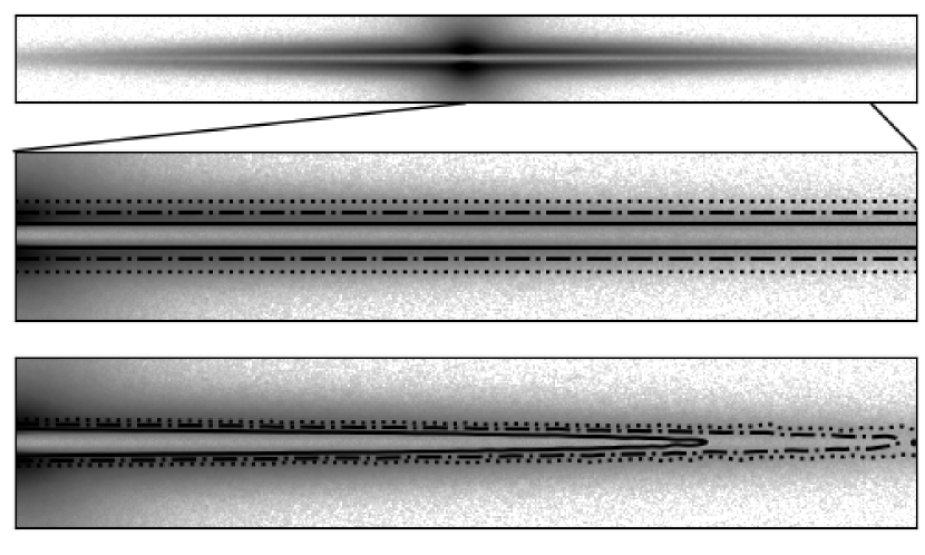
Figure 1: Top panel: an $r$-band image of a galaxy model with a face-on optical depth $\tau=1$. Middle panel: the same model enlarged with lines showing areas that would be covered by a flat mask with various $h_{\mathrm{mask}}$ values (see text): 2, 4, and 6 for solid, dot-dashed, and dotted lines respectively. Bottom panel: the same but with lines showing areas that would be covered by a relative mask for various $f_{\mathrm{mask}}$ values: 0.1, 0.25, 0.5 for dotted, dot-dashed and solid lines.

The appropriate size of the flat mask depends on the absorption strength. Even with the fixed values of $z_{\mathrm{disc}}$ and $z_{\mathrm{dust}}$, the area where the dust impact is significant depends on the value of $\tau$. This is illustrated in Fig. 2 by a vertical slice made through the center of an image for a dust-free model and for a set of models with an increasing value of $\tau$. It can be seen from the figure that, while for galaxies with a relatively small dust content a flat mask with $h_{\mathrm{mask}}=1$ (i.e. height of a mask equal to $z_{\mathrm{dust}}$) may cover the affected areas of the image well enough, galaxies with prominent dust lanes require that the mask should be several times wider. We also note that from this figure it becomes clear that even relatively transparent discs in a face-on orientation (with $\tau=0.1$) demonstrate a prominent dust lane in an edge-on orientation; a central peak on the slice is completely obscured by the dust and a darker depression is visible instead.

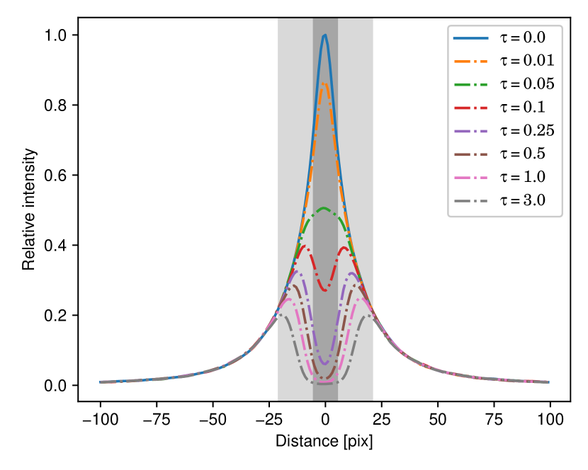
Figure 2: The impact of dust on the light distribution in a galaxy mock image illustrated by a vertical slice made through the image centre. Solid line: a dust-free ($\tau=0$) model. The dot-dashed lines show the set of models with increasing values of $\tau$. The darker shaded region shows a distance of $z_{\mathrm{dust}}$ from the model mid-plane, a lighter one – a distance of $4z_{\mathrm{dust}}$.

The drawback of using the flat mask is that it covers the mid-plane of a galaxy evenly for all radial distances from the galaxy centre, whereas most of the attenuation happens in the central region of a galaxy and decreases towards the periphery. This means that a mask that has a larger height in the central region of a galaxy and becomes thinner toward the galaxy edges would more efficiently cover the dust-affected regions of the galaxy. The exact shape of such a mask is not easy to find, as it depends on the complex interplay between the parameters of the stellar and dust components. Luckily, when we work with simulations, it is possible to determine the optimal parameters of such masks numerically. By comparing a mock image of a modeled dusty galaxy to an image of a model with the same stellar components but without dust, we can find regions of the dusty model that are most affected by the dust attenuation to mask them out. This leads to another masking strategy (we will call it a “relative” mask): a mask that covers the regions where the relative change between the models with and without dust is higher than a given threshold. The relative mask likewise has one free parameter to vary, the relative change between the two models $f_{\mathrm{mask}}$ above which we start our masking (in other words, a relative mask with $f_{\mathrm{mask}}=0.5$ covers regions where the dust attenuation is higher than 50%). The areas that are covered by a relative mask with $f_{\mathrm{mask}}$ values of 0.1, 0.25, and 0.5 are shown in the bottom panel of Fig. 1. It can be seen that the relative mask covers the dust-affected regions of a galaxy more effectively: it is wider near the galaxy centre and becomes thinner outwards. Another illustration of a comparison between these two approaches for creating dust masks is shown in Fig. 3. This figure shows the fraction of the total galaxy area (defined here as an image region that contains 99% of the total model flux) covered by different masks as a function of $\tau$. Since flat masks do not depend on $\tau$, instead only depending upon $z_{\mathrm{dust}}$, their covered area appears as a flat strip. Relative masks, in contrast, depend on $\tau$ and grow as the absorption increases. From this figure it is clear that the relative masking method is a more efficient way to cover the dust lane in terms of the fraction of the galaxy image that is left for the upcoming fitting. As it will be shown later in Sec. 3, this leads to considerably better fitting results in terms of the precision of the recovered galaxy parameters.

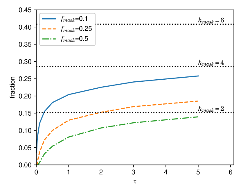
Figure 3: Fraction of the galaxy covered by masks of different types as a function of the dust disc optical depth $\tau$. Horizontal dotted lines show three flat masks, and the three curved lines show the behaviour of relative masks.

Although the relative masking approach appears to be more promising, such a mask can be created easily only in the controlled conditions of a numerical experiment. In practice, one cannot readily find the relative fraction of light absorbed by dust for every pixel of a galaxy image. To make this approach applicable to conditions where there is no such information available (i.e. in real observations), we decided to train a neural network to produce a relative dust mask based on optical images of a galaxy.

2.4.2 Neural networks for mask creation

A relative mask represents a binary image where pixels with a value of 1 define a masked region in the corresponding galaxy image and pixels with a value of 0 define the unmasked region. A generation of such masks from galaxy images in several optical bands is the semantic segmentation problem. To tackle it, we employ a U-Net (Ronneberger et al., 2015) based network that was successfully used in Smirnov et al. (2023) to solve the Galactic cirrus segmentation problem in SDSS optical bands.

The family of U-Net-based neural network models has been applied in various fields of science. These network architectures are employed in medicine (Iglovikov et al., 2017b; Ching et al., 2017; Ing et al., 2018; Andersson et al., 2019; Nazem et al., 2021), biology (Kandel et al., 2020), satellite image analyses (Iglovikov et al., 2017a), and astronomy (Aragon-Calvo, 2019; Bekki, 2021; Bianco et al., 2021; Wells & Norman, 2021; Vojtekova et al., 2021; Różański et al., 2022; Zavagno et al., 2023).

As the name suggests, the U-Net network model consists of two opposite paths. The down-sampling part, often called the encoder, is used to capture features from an input image. The encoder consists of several repeated blocks of convolution and max-pooling operations like in a typical convolutional neural network. The up-sampling part, often called the decoder, is used to get precise localisations. The decoder also consists of repeated blocks of an up-sampling (increasing the resolution) of the feature map followed by convolution operations. Therefore, the spatial resolution of the tensor processed in the decoder increases. To get a localisation, the features from the encoder are concatenated with the up-sampled features from the decoder via skip connections.

Our neural network model is implemented in the TensorFlow2.x framework (Abadi et al., 2015). The key difference between our solution and the original U-Net architecture is the encoder. As the encoder, we used the MobileNetV2 network model (Sandler et al., 2018), which is more lightweight than the original U-Net encoder, but has demonstrated a similar performance in the Galactic cirrus segmentation problem (Smirnov et al., 2023). Fig. 4 displays the encoder-decoder architecture used.

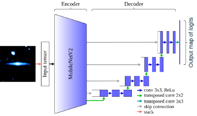
Figure 4: The encoder-decoder architecture used in this study.

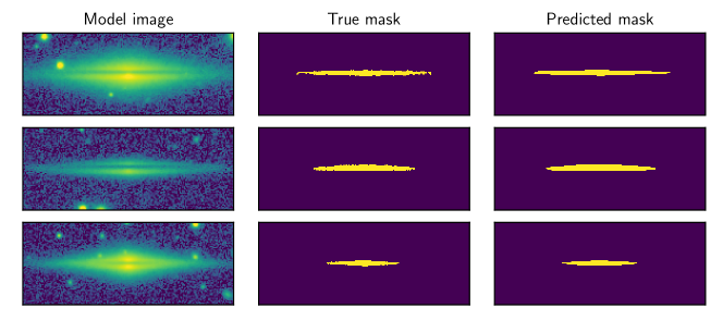
Figure 5: An example of using the neural network model for three simulated edge-on galaxies. Left panels: images of simulated galaxies in the $r$-band; middle panels: the corresponding relative mask ($f_{\mathrm{mask}}=0.3$) computed from the model; right panels: masks generated by the neural network model. Background stars on the model images are from random SDSS fields (see text).

During training experiments, we found accurate neural networks for different relative masks (ones with various $f_{\mathrm{mask}}$ values). We created separately trained networks for a set of $f_{\mathrm{mask}}$ values equal to 0.1, 0.3, 0.4, and 0.5. The data preparation to train the neural networks and the results of training experiments are described in Appendix A.

To find the best neural network to reproduce each relative mask, we use the IoU metric for the masked regions:

$$\mbox{IoU~{}}=\frac{\mbox{TP}}{\mbox{TP}+\mbox{FP}+\mbox{FN}}\,,$$ (9)

where TP is the number of true positive pixel results where the network correctly predicts the masked pixel, FP is the number of false positive pixel results where the network predicts the masked pixel but it belongs to the unmasked region, FN is the number of false negative pixel results, where the network predicts the unmasked pixel but it belongs to the masked region.

As demonstrated in Fig. 5, the relative mask generated by our network quite accurately reproduces the original relative mask. Note that for galaxies which are aren’t viewed perfectly edge-on and where the dust lane is shifted with respect to the galaxy center due to the projection effects, the mask generated by the neural network is also shifted and bent accordingly (see the second row in Fig. 5).

Quantitative results for different networks and training methods are shown in Table 5. We summarise the results of our experiments as follows.

1. As one can see in Table 5, the best networks for all considered relative masks have a similar performance ($0.838\leq$ IoU $\leq 0.847$).

2. Networks trained using the «fine-tuning» strategy demonstrate the best IoU per generation of all relative masks excluding a relative mask with $f_{mask}=0.4$, but, as one can see in Table 5, the advantage of these networks over ones trained from scratch or using the «transfer learning» strategy is insignificant.

3. Our networks generate relative masks for a thousand galaxies in about 80 seconds when running predictions on an AMD Ryzen 9 3900X 12-Core CPU and about 40 seconds when running on an NVIDIA GeForce RTX 3060 GPU.

2.4.3 Model with a dust component

The second approach in accounting for the dust’s impact during the decomposition process that we test in this work is modifying the fitting model such that it includes a dust component. The correct treatment of this problem requires heavy and time consuming computations both of light absorption and of scattering by dust grains. Moreover, such computations are often based on a Monte-Carlo approach, so they introduce some randomness into the model computations. This can impede using minimisation techniques based on gradient computations which are often used in decompositions.

One simplification that can be made is neglecting light scattering, so that the only cause of losing photons is absorption. While scattered light can be important in disc galaxies, especially for near face-on orientations (Byun et al., 1994; Baes & Dejonghe, 2001; Gadotti et al., 2010), simulations show that for near edge-on orientations, the fraction of scattered photons in the observed flux declines (Pierini et al., 2004). If a photon is scattered vertically in the disc, there is a high probability it leaves the galaxy and cannot be observed from an edge-on orientation. If a photon is scattered along the disc plane, where the optical depth is high, it will most likely experience another interaction with the dust to being either absorbed or scattered away from the disc plane.

Under these conditions, the model flux at a given pixel $(x,y)$ can be found as a line-of-sight integral which includes the optical depth term: for each point along the line-of-sight, we need to integrate over the dust density between this point and the observer’s position to compute the absorption for photons emitted at this point:

$$I(x,y)=\int_{-\infty}^{+\infty}\rho_{\mathrm{stellar}}(s)e^{-\int^{s}_{-\infty}\kappa\rho_{\mathrm{dust}}(s^{\prime})ds^{\prime}}\,ds,$$ (10)

where $\rho_{\mathrm{stellar}}(s)$ is the total luminosity density of a stellar model at a given point along a line-of-sight, $\rho_{\mathrm{dust}}(s)$ represents the dust density with the extinction coefficient $\kappa$, with the negative line-of-sight direction being towards the observer. In this case, the dust term accounts for the decrease in observed photons due to both absorption and scattering away from the plane of the disc.

To implement this approach, we modified the IMFIT code, by adding a new component function that represents a combined model with a disc, bulge, and dust. The necessity to compute a double integral for every pixel of an image is a drawback for this method, since it imposes a high computational cost on the decomposition. On the other hand, it is more physically realistic than, for instance, a disc with a negative flux that was used to model a dust lane in Savchenko et al. (2017) and Smirnov & Savchenko (2020). Another advantage of implementing an approach with the direct integration in IMFIT is that there is no need in Monte-Carlo simulations in our computations. As a result, a Poisson noise that depends on the number of photon packages is not introduced in the results. Therefore, the output model image is smooth and can be compared with the input galaxy image using standard minimization techniques that involve computations of the numerical derivatives of $\chi^{2}$ (such as the Levenberg–Marquardt algorithm). Images obtained via Monte-Carlo simulations are noisy and different realizations of the same model can have slightly different $\chi^{2}$ values which impedes a gradient computation in the fitting procedure, and some other minimization technique is required (such as a genetic algorithm which does not rely on gradient computations but takes a lot more computational time). Using an AMD Ryzen 7 3700X 8-Core Processor, it takes less than 10 seconds to obtain a model image of a dusty galaxy with a size of $500\times 500$ pixels using our modified IMFIT code.

3 Results of simulations

In this section we present the results of our simulations. To demonstrate how the dust distorts the measured values of the decomposition parameters, we make plots where the measured value of a parameter is plotted against the face-on optical depth $\tau$. These plots contain both decomposition results without dust correction and those obtained with using different strategies to account for the dust (see Sec. 2.4), so that their outcomes can be compared. Similar simulations made by Gadotti et al. (2010); Pastrav et al. (2013a, b) were performed for $\tau$ values up to 8, but the recent study by (Mosenkov et al., 2018) shows that the total face-on absorption in disc galaxies does not reach such high values; the mean measured value for their sample of seven edge-on galaxies was found to be around $\tau=1$ in the $V$ band and the highest measured value was 2.01 for NGC 5907. On the other hand, galaxies with a higher amount of dust may exist, so we test our approaches of taking the dust into account in most extreme conditions with different possible $\tau$ values. Therefore, we decided to increase the investigated range of $\tau$ values well above the observed $\tau=2.01$ and set $\tau=5$ as an upper limit for our computations.

Also, we explore how different galaxy models (for example, with different bulge-to-total luminosity ratios or different relative stellar-to-dust disc scale heights) are affected by the dust component with various optical depths.

Before proceeding to the results of simulations, we need to mention that the obtained discrepancies between the true values of the parameters and the ones that we infer via decomposition actually have two origins. The first is obviously the influence of dust, whereas the second is some intrinsic decomposition biases. As was previously found in Gadotti et al. (2010); Pastrav et al. (2013a, b), even if dust is absent in a model, the measured decomposition parameters can differ from their true input values. In those studies, this difference was attributed to a mismatch between the models. While the radiative transfer model used for the image creation was three-dimensional, the decomposition model contained a simple two-dimensional exponential disc. This two-dimensional model cannot take the disc’s vertical structure into account, which results in an increase of the disc’s inclination. For the edge-on galaxies where the disc thickness plays a dominant role, the two-dimensional exponential model cannot be applied to infer disc properties, since the projected light distribution in this case is not exponential, but can be described as a combination of a Bessel and hyperbolic secant function (van der Kruit & Searle, 1981).

In this paper, we also find that the results of the decomposition via dust-free models do not exactly match the values of the input parameters, especially for the bulge component. A possible explanation for this error is the presence of the noise we added intentionally to our mock images. This noise has two sources. The SKIRT code operates in terms of photon packages that are emitted inside the galaxy and then propagate through the galaxy body towards the observer. Since the number of such packages is finite, a model image is not smooth, but demonstrates some photon noise. The second source of the noise is the one we added to convert a SKIRT simulated image to an “observed” image. In this work, we model images of the $r$-band of the SDSS survey, therefore, we use the noise characteristics of this instrument (see Sec 2.2).

To examine how these two noises impact our decomposition results, we run a number of fits with different noise parameters. First, to study how the number of photon packages in a SKIRT simulation affects the decomposition quality, we create the same model but with $10^{6}$,  $5\cdot 10^{6}$, and $10^{7}$ photon packages and then decompose these models using the same technique. To inspect the impact of the included camera noise, we run these three simulations with a different number of photon packages twice: with and without adding the camera noise. The results of these experiments are listed in Table 2, where the measured value of the Sérsic index is shown along with the true value of 4.0. One can see that the measured value is almost unaffected by the number of photon packages, while adding the camera noise makes a significant change to the retrieved parameters. The fact that even for a noise-free model we do not recover the correct value of the Sérsic index, but have a somewhat lower value, probably originates from an interference between the bulge and disc components that overlap in the image which leads to a degeneracy of their parameters.

From these simulations, we make a conclusion that the added camera noise is the main source of error when decomposing a dust-free galaxy image, and that all follow-up experiments with dusty models also include this bias. Since our main goal is to simulate the decomposition errors for real observations (which always contain noise), we do not correct our results for this bias, but emphasise that the estimated decomposition errors can have various reasons apart from the dust impact which we discuss in detail in the next sections. All simulations in the subsequent sections are made for the SDSS $r$ band.

Photon packages	$10^{6}$	$5\cdot 10^{6}$	$10^{7}$
With camera noise	3.46	3.44	3.44
Without camera noise	3.88	3.86	3.86

Table 2: Measured bulge Sérsic index for a set of decompositions with different noise parameters.

3.1 Dust impact on the bulge parameters

The bulges of disc galaxies show a peak intensity at their centres and, generally, a rather swift decrease in their surface brightness in their outer regions. As shown in Gadotti et al. (2010), even for galaxies with inclinations far from an edge-on orientation, the bulge parameters can be strongly affected by dust. To demonstrate how the dust component affects the fit parameters of the bulge in an edge-on orientation, we run our algorithm for three models with different bulge parameters: a big, medium, and small bulge (their parameters are listed in Table 3). We note that all models have the same value of the Sérsic index equal to 4 (i.e. they represent de Vaucouleurs bulges). Bulges with different Sérsic indices have different concentrations and, thus, it is natural to expect that the presence of dust affects their measurements differently, but in this article we do not consider this problem. The disc parameters of these models are the same as in the basic model (Tab. 1).

Model	$r_{e}$ [pc]	$n$	$q$	$B/T$
Small	700	4	0	0.1
Medium	900	4	0	0.2
Big	1500	4	0	0.3

Table 3: Parameters of the three models corresponding to the different bulges.

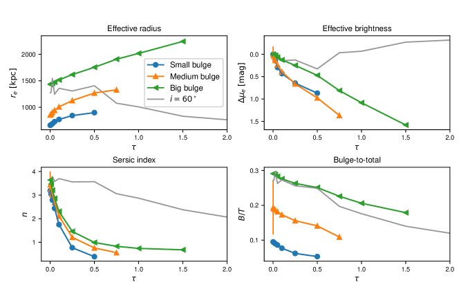
Figure 6: The dependence of the measured bulge parameters’ values on the face-on optical depth $\tau$ for the effective radius, effective surface brightness, Sérsic index, and bulge-to-total luminosity ratio. Three bulge models are shown: a “small bulge” model ($r_{e}=700$ pc, $B/T=0.1$), “medium bulge” model ($r_{e}=900$ pc, $B/T=0.2$), and “big bulge” model ($r_{e}=1500$ pc, $B/T=0.3$). The grey line shows the results for a “big bulge” model with an inclination of 60 degrees.

Fig. 6 demonstrates how the measured values of the bulge’s effective radius, effective surface brightness, Sérsic index, and bulge-to-total luminosity ratio depend on the amount of dust in the model. From this figure, we note that when a galaxy is viewed edge-on, the bulge parameters deteriorate very quickly as the optical depth of the dust component increases. Although we run our simulations for a range of $\tau$ from 0 to 5.0, in all three models, the bulge component begins to diverge long before reaching the maximal value of $\tau$. For example, the small bulge model collapses to the lower limit of the Sérsic index at $\tau\approx 0.5$; after that point the gradient descent algorithm starts to converge to random values around the initial conditions. This indicates that the bulge is obscured to such a great degree that it does not affect the total value of the $\chi^{2}$ statistics. The same happens for the medium bulge model at $\tau\approx 0.75$ and for the big bulge model at $\tau\approx 1.5$. Since all the bulge models have collapsed by $\tau\approx 1.5$, we do not show the results of modelling higher absorptions in this figure.

For smaller values of $\tau$, where we managed to obtain at least some measurable values for the bulge parameters, their behaviour is similar in each model. The fit effective radius of the bulge grows with optical depth, which can be easily understood from a geometrical point of view: the central peak of the bulge is obscured, but its outer regions (outside of the plane of the disc) are essentially unaffected. Thus the radius where half of the total observed bulge flux is confined must be larger than in the dust-free case. The observed Sérsic index decreases for the same reason: the obscured central peak leads at a flatter apparent surface brightness distribution, i.e. lower values of $n$. For the small bulge model, the measured value of the Sérsic index drops from a true value of 4.0 to a value of 2.0 already at $\tau\approx 0.075$, which value of $\tau$ corresponds to when the dust component begins to appear as a darker lane in the galaxy image (see Fig. 2). Therefore, even if a visual inspection does not reveal a dust lane in a galaxy, it can still contain enough dust to render the parameters of a small bulge completely distorted. This in turn affects some standard galaxy scaling relations, which contain the parameters of the bulges (e.g. the Kormendy relation), or, for example, make the “classical bulge – pseudobulge” dichotomy less pronounced.

The other two panels in Fig. 6 show the results for the effective surface brightness (in terms of its difference from its true value) and the observed bulge-to-total luminosity ratio. There is no surprise that for models with a higher dust content, our measurements show progressively fainter bulges, although for the bulge-to-total luminosity ratio, the changes are not as extreme as for the Sérsic parameter. This happens probably because the disc component is also obscured by the dust and this suppresses the total $B/T$ ratio shift to some level.

For comparative purposes, Fig. 6 also displays the results of our simulation for the big bulge model inclined by 60 degrees. The result of this simulation closely follows the results reported in Gadotti et al. (2010) where this inclination was the highest among those they considered: the effective radius, Sérsic index, and bulge fraction all decrease with optical depth (see their figures 3 and 4), which validates our simulations. It is clear from this comparison that for the edge-on orientation, the impact of the dust on the bulge parameters is disparately higher than for mildly inclined galaxies. We note that the difference between the edge-on and non-edge-on cases is not solely quantitative, but a contrasting behaviour can be observed instead. For the edge-on models, the measured value of the bulge effective radius tends to be higher then the true one, whereas for a mildly inclined model it becomes lower. The same behaviour was also confirmed for models with exponential and de Vaucouleurs bulges (Pastrav et al., 2013b) for a wide range of inclinations, from face-on to almost edge-on, but for decomposition with infinitely thin discs.

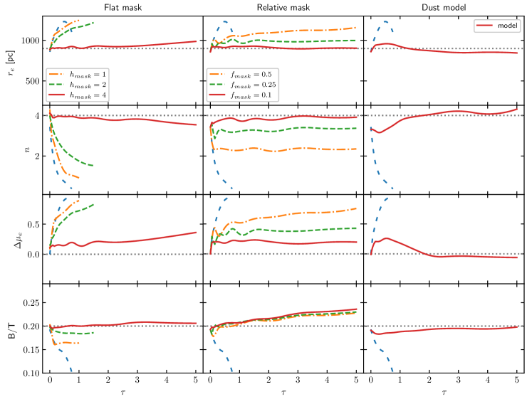
Figure 7: Results of fitting with dust correction methods for the bulge parameters. Each panel shows the measured value as function of $\tau$. The top row shows results for the effective radius $r_{e}$, the second row shows the Sérsic index $n$, the third one shows the error of the effective surface brightness $\Delta\mu_{e}$, and the bottom row shows the measured bulge-to-total luminosity ratio. Different dust correction techniques are shown in the columns: the leftmost column shows the decomposition with flat masks with $h_{\mathrm{mask}}=1$ (dot-dashed line), $h_{\mathrm{mask}}=2$ (green densely dashed line), and $h_{\mathrm{mask}}=4$ (solid line); the middle column shows relative dust masks with $f_{\mathrm{mask}}=0.5$ (dot-dashed line), $f_{\mathrm{mask}}=0.25$ (green densely dashed line), and $f_{\mathrm{mask}}=0.1$ (red line); the rightmost column shows the results of decomposition with a dust model (red line). For comparison, each panel shows the uncorrected values (blue sparsely dashed line) and the true values as a grey dotted level.

Fig. 7 shows the decomposition results for the middle bulge model with the aid of various techniques for taking the dust into account. There are four bulge parameters shown in this figure (the effective radius $r_{e}$, the Sérsic index $n$, the error of the effective surface brightness $\Delta\mu_{e}=\mu_{e}^{\mathrm{measured}}-\mu_{e}^{\mathrm{true}}$, and the bulge-to-total ratio B/T) and three dust correction methods (the flat mask, relative mask, and dust model), for a total of twelve panels. The columns show different methods, the rows, different parameters. Each panel also contains results for the uncorrected decomposition (the same as in Fig. 6) for comparison purposes, and the true value of each parameter marked as the horizontal dotted line. Below we describe all three approaches for the dust correction separately.

Flat mask

The results of the decomposition with flat masks are shown in the leftmost column of Fig. 7 for three mask sizes: $h_{\mathrm{mask}}=1,2,\mbox{and }4$ (a yellow dash-dotted line, a green dashed line, and a red solid line, respectively), along with the results of the unmasked decomposition (the blue sparsely dashed line). As we discussed earlier, without dust correction the bulge model collapses at $\tau\approx 0.75$. The same happenes for decomposition with a relatively narrow flat mask: for a mask with $h_{\mathrm{mask}}=1$, the model collapses at $\tau\approx 1$, and for $h_{\mathrm{mask}}=2$ at $\tau=1.5$. Therefore, the narrow flat mask provides almost no improvement compared to the unmasked case: the decomposition results become highly distorted even for low values of $\tau$.

For a wider mask ($h_{\mathrm{}}=4$), the results are considerably better. Even though all three parameters still deviate from their true values, this deviation is confined in a narrower range, and moreover, the model converges successfully for all considered $\tau$ levels up to 5.0. There is still an apparent systematic shift in all three parameters in the same direction as for the decomposition with narrower masks, but for a moderate dust content it is not larger than typical uncertainties for decomposition results.

Relative mask

The middle column in Fig. 7 shows the results of the decomposition with three relative masks: $f_{\mathrm{mask}}=0.5$, $f_{\mathrm{mask}}=0.25$, and $f_{\mathrm{mask}}=0.1$ (a yellow dash-dotted line, a green dashed line, and a red solid line, respectively). The first fact that should be noted is that the results of the decomposition with the relative mask are better than both those without any masking and with a flat mask.

For a model with $\tau=1$, the total area that is covered by the relative mask with $f_{\mathtt{mask}}=0.5$ is almost the same as the flat mask with $h_{\mathrm{mask}}=2$ (in fact, it is 10% smaller, see Fig. 3), so the green curve in the left column can be directly compared to the yellow curve in the middle one to assess the performance improvement of the relative mask. It is clear that despite having virtually the same total covered area, the relative mask does a better job in reducing the dust impact on the decomposition results. The same is true for all tested values of $\tau$: the relative mask allows us to recover the bulge parameters more reliably while covering a smaller fraction of the galaxy image.

Dust model

The results of applying our combined IMFIT model – which contains a bulge, disc, and dust component – to decompose a synthetic image are shown in the right column of Fig. 7. This decomposition does not employ any masking, and taking the dust into account only happens by including the dust term during the line-of-sight integration (Eq. 10) for the model. The figure suggests that the performance of this approach is comparable with the results of the widest flat ($h_{\mathrm{mask}}=4$) and relative ($f_{\mathrm{mask}}=0.1$) masks.

Our inability to recover the precise values of the structural parameters when utilizing this approach can be attributed to two facts: i) it does not include the light scattered by the dust, and ii) it reflects the general problems of a decomposition with a complex model, where a degeneracy between some parameters can occur and lead to a systematical shift in parameters (Gadotti et al., 2010).

Although the dust model technique does not show considerably better results when compared with dust masking, whilst taking an order of magnitude longer in computation time, it still has an advantage in that it does not lose information about the galaxy by masking out some galaxy regions. If a galaxy has a more complex structure, such as two (thin + thick) stellar discs, the thin disc can be completely covered by a dust mask, whereas the dust model approach can still recover the disc structure with some accuracy.

3.2 Stellar discs

Since the dust disc is embedded inside the stellar disc, it is natural to expect that the impact of dust on the fit disc parameters should depend on the scaling relations between the structural parameters of the two discs. To investigate this, we ran simulations for a set of various dust disc parameters while keeping the stellar disc parameters fixed to those given in the basic model (Table 1).

The first set of simulations regards a relation between the radial scale lengths for the stellar and dust discs. Observations show that there is a correlation between the radial scale length of the emission profile at 3.4 $\mu$m (which traces the bulk of the stellar mass in a galaxy) and that at 100 $\mu$m (which is dominated by the emission of cold dust, Mosenkov et al. 2022b, see also Mosenkov et al. 2019 for a similar correlation but for the effective radius). Moreover, Casasola et al. (2017) found for 18 face-on spiral galaxies the following ratio between the disc scale lengths of the stellar and dust surface density distributions $h_{\Sigma\mathrm{dust}}/h_{\Sigma\mathrm{star\,3.6}\mu\mathrm{m}}=1.80\pm 0.13$ which is generally consistent with the results from radiative transfer modeling (Mosenkov et al. in prep.). In this study, we decided to consider three possible situations: a dust disc which is slightly shorter than a stellar disc ($h_{\mathrm{dust}}=3000$ pc – some galaxies harbor a shorter dust disc than their stellar disc, e.g. NGC 4013, Mosenkov et al. 2018), both discs having the same radial scale ($h_{\mathrm{dust}}=4000$ pc), and a dust disc which is more extended than a stellar disc ($h_{\mathrm{dust}}=5000$ pc), to see if these differences translate into various systematical shifts in the derived parameters.

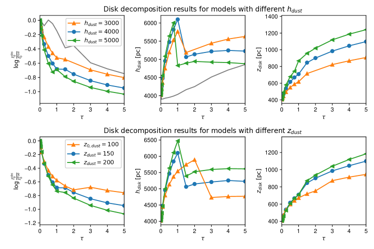
Figure 8: Disc parameters retrieved by decomposition for a set of models with different dust disc parameters. Top row: results for the disc central surface brightness (left panel), radial exponential scale (middle), and vertical scale (right) for three dust components with a radial scale shorter, equal to, and larger than that of the stellar disc. For comparison, the grey lines for the panels about surface brightness and exponential scale show results for the same disc with $h_{\mathrm{dust}}=4000$ pc, but with an inclination of 60 degrees. Bottom row: the same parameters obtained for dust models with different vertical scales ($z_{\mathrm{dust}}=$ 100, 150, and 200 pc).

The results of these simulations are demonstrated in the top row of Fig. 8. The values of the measured parameters are shown as a function of the face-on dust optical depth $\tau$. The left panel shows the observed central surface brightness in terms of a decimal logarithm of a fraction of the observed to true value, without dust attenuation. The middle panel shows the measured radial exponential scale of the stellar disc. The right panel shows the measured value of its vertical scale. For comparison, in the panels with surface brightness attenuation and radial scale we also show the results of simulations for a basic model inclined at 60 degrees. Again, the results of decomposition with the inclined disc, in general, follow the results presented in Gadotti et al. (2010), and for the edge-on orientation, the impact of the dust on the disc parameters is higher.

From these plots it is clear that the dust component severely changes the observed values of the stellar disc. All three models show a similar behaviour for the observed central surface brightness: its value drops quickly to about 20% the original level at $\tau\approx 0.5\div 0.75$, and then after a short pause a shallower attenuation is observed. A possible explanation for this behaviour is that at these values for the face-on optical depth, the edge-on disc absorption exterminates almost all observed photons near the galaxy midplane, and then the following attenuation occurs in regions far from the disc plane where the dust content is lower. From this plot it can also be seen that the general behaviour of the attenuation in edge-on discs follows the what’s seen in inclined discs, although in edge-on discs it is qualitatively stronger.

A different picture is seen for the disc radial scale length (top-middle panel). While for a disc inclined at 60 degrees the fit value of this parameter gradually increases with $\tau$ and reaches a relative change of 10% only at $\tau\gtrsim 2$ (i.e. this disc would demonstrate a very prominent dust lane if observed in an edge-on orientation), for an edge-on disc a very sharp increase is observed. In this case, at the same value of $\tau\approx 1-1.5$, the relative change of the $h_{\mathrm{disc}}$ reaches a peak that is approximately 50% higher than the true value (a similar $\approx 50\%$ increase of the observed values of $h_{\mathrm{disc}}$ was reported for an (almost) edge-on orientation, but for decomposition with an infinitely thin disc). After that, the observed value of $h_{\mathrm{disc}}$ quickly drops to $\approx 5000$ pc (25% higher than the true value), and its behaviour for higher $\tau$ depends on the relation between $h_{\mathrm{dust}}$ and $h_{\mathrm{disc}}$. If $h_{\mathrm{dust}}<h_{\mathrm{disc}}$, the curve of the measured value for $h_{\mathrm{disc}}$ starts to grow again. If $h_{\mathrm{dust}}\geq h_{\mathrm{disc}}$, it appears to be more stable and does not change appreciably for a wide range of $\tau$.

The observed break at $\tau\approx 1.5$ in the plot for $h_{\mathrm{disc}}$ (top-middle plot of Fig. 8) is caused by issues with the bulge fitting. For high absorption levels, the Sérsic component cannot fit the bulge properly because the dark dust lane in the galaxy midplane suppresses its maximal brightness. This leads to the appearance of two under-fit bulge “remnants” above and below the disc plane, where the bulge protrudes from the dusty disc. Their fraction in the residuals increases with $\tau$ because the bulge fit becomes progressively worse and the disc itself becomes darker due to absorption, while these bulge regions remain almost unobscured. At some point, it becomes more efficient for the model (in terms of its achieved $\chi^{2}$ value) to fit these bulge remnants as part of the disc component. This leads to a more concentrated disc model and, therefore, a shorter radial scale.

The results for the last disc parameter, its vertical scale height $z_{\mathrm{disc}}$, are shown in the top-right panel of Fig. 8. Again, all three models show the same general trend in that the fit value of $z_{\mathrm{disc}}$ increases with $\tau$. This is easy to understand since the dust absorbs more photons close to the disc plane, making the vertical brightness distribution flatter, therefore it can be approximated with a higher value of $z_{\mathrm{disc}}$. We also point out a clear systematic trend: the larger the dust exponential scale height, the greater its impact on the observed $z_{\mathrm{disc}}$ value. Since in both Gadotti et al. (2010) and Pastrav et al. (2013a, b), an infinitely thin disc model was utilized during decomposition, the $z_{\mathrm{disc}}$ value was not inferred in their simulations and our results cannot be compared with these studies.

The bottom row of Fig. 8 shows the results of our simulations with different $z_{\mathrm{dust}}$ values. One can see that, in general, the behaviour of all three parameters are the same as those obtained for models with varied $h_{\mathrm{dust}}$ values. We note that all else being equal, a thicker dust disc leads to more distorted stellar disc parameters.

Flat mask

In this and the next two paragraphs, we describe the results of taking the dust into account using three various techniques in a similar way as it was done for the bulge. We begin with a flat mask approach, which results are demonstrated in the left column of Fig. 9. The figure shows that while a flat mask allows one to enhance the quality of the decomposition, only a mask that is four times wider than $z_{\mathrm{dust}}$ yields parameter estimates that are close to their true values. Narrower masks result in a systematic shift in the parameters (a rapid decline of the disc flux, and an increase in both the radial and vertical scales) that depend on the value of $\tau$.

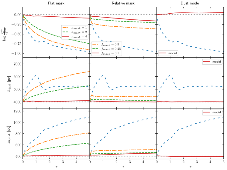
Figure 9: Results of the fitting with different dust correction methods for the disc parameters. The general structure of the figure follows similarly to the bulge decomposition results (see the caption of Fig. 7), except for the disc parameters, the rows correspond to the central surface brightness (top), the radial scale (middle), and the vertical scale (bottom).

Relative mask

For retrieving disc parameters, a relative mask (middle column of Fig. 9) provides better results than a flat mask. Even the mask with the smallest covered area ($f_{\mathrm{mask}}=0.5$) gives estimates of the radial and vertical disc scales closer to the true values when compared to the considerably larger flat masks. However, the central surface brightness is still systematically underestimated. The most extended relative mask ($f_{\mathrm{mask}}=0.1$) allows us to recover the radial exponential scale almost perfectly, although for this value, there are some trends present in the central surface brightness and the vertical scale. Their errors are comparable to the characteristic uncertainties of the decomposition. We conclude that, as is the case for the bulge parameters, a disc decomposition with a relative mask generally gives better results for some fixed fraction of the covered galaxy image.

Dust model

The right column of Fig. 9 shows the results of a decomposition using a model with a dust component. This approach allows us to almost perfectly recover both the radial and vertical exponential scales, and there is only a slight overestimation of the disc central surface brightness. The fact that our model allows us to retrieve almost exact values for the disc parameters even for a high dust content seems to confirm the fact that light scattering has little impact on galaxy decompositions in an edge-on orientation, as was mentioned by Pierini et al. (2004). Also, for an the edge-on orientation, the spatial overlap between the disc and bulge components is lower, which reduces the degeneracy of their parameters.

4 Demonstration on real galaxies

In previous sections, we described the techniques we used to account for a dust component and the results of their application to synthetic images of several model galaxies. To further validate these approaches in inferring the structural parameters of disc galaxies, we present the results of decompositions for a couple of real edge-on galaxies. We use two methods to account for the dust component: a neural-network generated relative dust mask, and an IMFIT-model with a dust component. For this purpose, we selected two edge-on galaxies with prominent dust lines but without significant complex features in their discs (warps, flarings, bright halos, etc.) from the EGIPS catalog, which contains a sample of 16551 edge-on galaxies. The selected objects are PGC 27896 and PGC 2441449. We downloaded their images from the Pan-STARRS1 survey (Chambers et al., 2016; Flewelling et al., 2020) in the $i$-band.

To compare decomposition results with and without dust correction, we first decompose these galaxies using a photometric model consisting of a Sérsic bulge and a 3D exponential disc, along with taking a dust mask or a dust model into account. In all cases, we use the same PSF image that was obtained by fitting a Moffat function to a stacked image of bright isolated stars in the galaxy frame. We masked off background and foreground objects using a segmentation map produced by the SEXTRACTOR package (Bertin & Arnouts, 1996). The results of our decompositions are shown in Fig. 10; the left column is for PGC 27896, the right is for PGC 2441449. The top panels show the original images of these two galaxies in the $i$ band with yellow bars marking a 30″scale.

The second row in Fig. 10 shows images of the dust masks generated by our neural network for the $f_{mask}$ parameter value equal to 0.3. The next three rows show best model images for the simple decomposition (without dust correction) first, then for the decomposition with a dust mask, and finally the decomposition with a dust model. It is evident that while the two former models can, in general, reproduce the overall shape of the galaxy, they miss an absorption lane, while the later one demonstrate the presence of a dust lane that is a part of the model. We note that the galaxy PGC 27896 (left column) is not oriented perfectly edge on, but is slightly inclined which results in a shift of the dust lane below the visible disc centre and in an asymmetry of the obscured bulge region. Both of these features are reproduced by our model that has converged to an inclination value of 89 degrees.

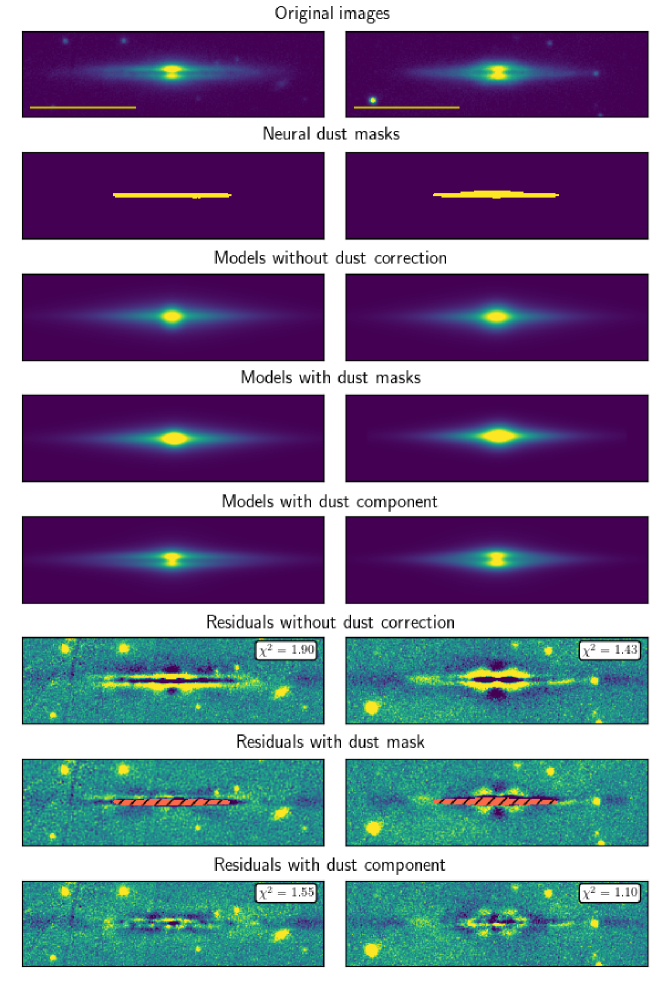
Figure 10: Decomposition of two real galaxies, PGC 27896 (left column) and PGC 2441449 (right column). Top panels: images of the galaxies in the $i$ band with 30″scale bars. Second row: dust masks created by our neural network. Third, fourth and fifth rows: best fit models for a decomposition without taking the presence of dust into account, with a dust mask, and with a dust model. Three bottom rows: residual maps for these decomposition approaches. Red hatched areas on the residuals with a dust mask show masked areas. The fit $\chi^{2}$ statistics is shown for decompositions without dust correction or with a dust component (the decompositions with the dust mask have a different masked area, so its statistics cannot be accurately compared with the other two methods).

The last three rows in Fig. 10 contain residual “image – model” maps for the three decomposition methods. The residuals for the decomposition without dust correction looks as expected, because the model converges to some averaged disc+dust solution, in the galaxy plane the models are too bright, resulting in the residual maps showing over-subtracted negative regions. Above and below the galactic plane, where the dust absorption is weaker, the model is too faint, which results in bright regions in the residuals. The residual maps for decompositions with a dust mask are different. Because the dust lanes of these galaxies are masked out, this does not lead to attenuated disc models, and a brighter disc appears instead. As a result, the residual maps show overly subtracted regions where the dust attenuation is high, but there are no bright regions above and below as in the previous case. This means that the disc model better fit low absorption regions of images.

The residuals of the decomposition with our new IMFIT model are shown in the bottom row of Fig. 10. They demonstrate a better agreement between the observed images and the corresponding models. While there are still some deviations from the zero level, they are considerably smaller. The dust lane is not overly subtracted and there are no bright regions around the disc plane. Although there are still slightly over-subtracted regions in the outer regions of the disc, they are attributed to the fact that both galaxies have Freeman Type II discs (Freeman, 1970), whereas in our models the disc is a pure exponential (Type I). In addition, Marchuk et al. (2022) catalogued these galaxies as having a B/PS bulge in the central part which is clearly visible in our residual images.

Numerical values for the decomposition results are listed in Table 4, where for both tested galaxies we present the fit structural parameters for a simple bulge+plus disc model (marked as “not corrected” in the table), for a decomposition with a dust mask (“dust mask”), and for our model with a dust component (“dust component”). One can see that for real galaxies we observe the same systematic shifts between the uncorrected and corrected values (see Figs. 6 and 8). After correction, the discs become brighter, thinner, and have shorter radial scales, whereas the bulges become brighter (with higher bulge-to-total luminosity values) and with larger Sérsic index values. We also mention that the results of the decomposition with a dust model have higher discrepancies with uncorrected parameters than the results of the decomposition with a dust mask. The latter appears to be somewhere in between the uncorrected parameters and the results of the decomposition with a dust model. This also aligns with the results of our numerical tests which demonstrate that the decomposition with dust masks of all kinds still has higher errors and systematical shifts when compared with the dust model decomposition. This is especially clear for the Sérsic parameters, which are almost the same as the uncorrected values.

		$\mu_{0,\mathrm{disc}}$	$h_{\mathrm{disc}}$	$z_{\mathrm{disc}}$	$\mu_{e}$	$r_{e}$	$n$	$B/T$
		$mag/\square^{\prime\prime}$	”	”	$mag/\square^{\prime\prime}$	”
PGC27896	Not corrected	20.00	9.8	2.2	20.8	2.19	0.4	0.12
	Dust mask	19.63	9.1	1.7	20.4	2.2	0.3	0.14
	Dust component	19.24	9.1	1.2	21.0	3.17	3.7	0.27
PGC2441449	Not corrected	20.26	8.9	2.1	21.33	3.3	0.6	0.19
	Dust mask	19.54	7.5	1.5	21.20	3.3	0.7	0.20
	Dust component	19.21	7.0	1.1	20.42	3.2	3.6	0.39

Table 4: Structural parameters of the two real galaxies recovered using a simple decomposition and the two methods of dust correction.

5 Conclusions

In this article we ran a number of numerical simulations in order to determine how the presence of dust impacts the measured values for the parameters of edge-on galaxies. To achieve this, we created a set of artificial galaxy images with various parameters and applied a standard decomposition method to them to be able to compare the input and output values of the structural parameters. We also tested three different techniques for how this impact can be minimized, two of which are based on masking dust attenuated regions of galactic images, and the third involves an analytical model that includes dust absorption. Our main conclusions can be summarized as follows.

We confirm the findings of previous authors (Gadotti et al. 2010; Pastrav et al. 2013a, b) who utilized two-dimensional decomposition to infer the general trends of how the bulge and disc parameters are altered due to the varied dust absorption. Using three-dimensional decomposition that accounts for the vertical structure of the stellar disc, we show that these trends hold true for perfectly edge-on galaxies, for which the disc thickness can not be neglected. For bulges, the measured values of the effective radius tend to be larger than the true (intrinsic) values, whereas the effective surface brightness, Sérsic index, and bulge-to-total luminosity ratio tend to be lower. In other words, bulges in dusty edge-on galaxies appear fainter and less concentrated than they really are. For discs, the measured values of the central surface brightness tend to be lower than the true values, while the radial and vertical scales tend to be larger. Therefore, discs also appear fainter and less concentrated than they are in reality. For both bulges and discs, the absolute values of the parameters’ shifts depend on the properties of these components and on the dust content in the galaxy.

Masking out the regions most affected by dust in a galactic image allows one to considerably reduce the dust’s influence and obtain better estimates of the galactic parameters. Comparing different masking techniques showed that a dust mask which is more extended in the center of the galaxy and is narrower in the outer region is better than a dust mask which has a constant width. A neural network can be trained to effectively generate such masks for images of real galaxies.

An analytical model that includes an absorbing dust component in a form of a 3D exponential disc can be used to perform decomposition of a galaxy with a prominent dust lane and infer the galaxy structural parameters corrected for dust. Even if this model does not include light scattering, for simplification, it performs better than any masking techniques that we tested.

The results of applying the proposed methods to a couple of real galaxies whilst taking the dust component into account are in agreement with numerical experiments and demonstrate the validity of our approach.

We plan to continue our research of the dust impact on the decomposition of galaxies, and consider other wavelengths (such as ultraviolet and infrared ranges) as well as other, more complicated galaxy models. We also plan to continue the development of different algorithms to correct the decomposition results for the presence of dust in galaxies that are viewed in an orientation close to edge-on.

Data availability

The data underlying this article will be shared on reasonable request to the corresponding author.

Appendix A Neural networks for relative mask generation

To train a neural network, one needs a dataset that can be split into training, validating, and testing subdatasets. To create such a dataset, we utilized the procedure based on the SKIRT package (see Sec. 2.2). Each sample consists of four images of the same size ($256\times 256$ pixels): three model images in the $g$, $r$, and $i$ passbands of the SDSS system that were used as a neural network input, and a ground truth image of a relative dust mask. To make our model images more realistic, we overlapped them with random fields from the SDSS footprint which added background objects and noise. The parameters of modeled galaxies were randomly chosen with a uniform distribution in the following ranges:

• bulge-to-total luminosity ratio: 0.05 – 0.35

• bulge effective radius: 500 – 1200 pc

• bulge Sérsic index: 0.5 – 5

• bulge ellipticity: 0.0 – 0.5

• stellar disc exponential scale: 2500 – 5000 pc

• stellar disc vertical scale: 0.1 – 0.3 of a stellar radial scale

• dust disc radial scale: 0.5 – 1.5 of a stellar disc radial scale

• dust disc vertical scale: 0.05 – 0.3 of a stellar disc vertical scale

• dust $\tau$ value: 0.1 – 5.0.

We also allowed models to have inclinations in a range of $\left[86:90\right]$ degrees to simulate galaxies that aren’t viewed perfectly edge-on.

Since different relative masks (with different $f_{\mathrm{mask}}$ values) can lead to different results for the decomposition (as we demonstrate by our experiments, see below), we used a set of $f_{\mathrm{mask}}$ values equal to 0.1, 0.3, 0.4, and 0.5 generate datasets to train several independent neural networks that predict masks with such parameters. In total, we created 10000 samples in each dataset to train our networks.

Each dataset was preprocessed in the same manner. Here we briefly provide the main data preprocessing steps.

1. We split the dataset into training, validating and testing as separate subdatasets of $8000/1000/1000$ images respectively.

2. Next, we calculated the common $99.9$th percentile values for each optical band ($g,r,i$) separately for the union of the training and validating subdatasets ($9000$ images). Then we applied corresponding clipping. This allowed us to moderate the problem associated with the brightest pixels which reduces the image contrast and decreases the training efficiency.

3. Then, we applied a natural logarithm transformation followed by min-max normalization to $\left[-1:1\right]$ range.

To train our neural network, we employed a sparse categorical cross-entropy loss function derived from the output tensor with logit function. To optimise the loss function, we chose the Adam optimization method. The batches consist of $32$ images. We trained all neural networks for $60$ epochs on a single NVIDIA GeForce RTX 3060 GPU. The lowest validation loss is reached in $30$-$40$ epochs.

During the training experiments, we varied 2 parameters that influence the fitting process and the final model performance: the training strategy («training from scratch», «transfer learning», or «fine-tuning») and the learning rate $r$. In the «transfer learning» strategy, we took a pre-trained ImageNet dataset (Deng et al., 2009) encoder and froze it before starting the training process. In the «fine-tuning» strategy, we also used a pre-trained encoder but did not freeze it.

Table 5: Results gathered from the conducted training experiments. This table lists the relative mask attenuation, training strategy («training from scratch», «transfer learning», or «fine-tuning»), learning rate, IoU, precision, and recall for all test galaxies for the relative mask class. The highest value for each metric is highlighted by the bold font for each relative mask.

$f_{\mathrm{mask}}$	Training strategy	$r$	IoU	precision	recall
$0.1$	training from scratch	$0.001$	$0.823$	$0.867$	$\mathbf{0.942}$
$0.1$	training from scratch	$0.0005$	$0.834$	$0.92$	$0.9$
$0.1$	training from scratch	$0.00025$	$0.826$	$\mathbf{0.936}$	$0.875$
$0.1$	training from scratch	$0.0001$	$0.822$	$0.923$	$0.882$
$0.1$	transfer learning	$0.001$	$0.833$	$0.929$	$0.89$
$0.1$	transfer learning	$0.0005$	$0.834$	$0.913$	$0.906$
$0.1$	transfer learning	$0.00025$	$0.834$	$0.913$	$0.906$
$0.1$	transfer learning	$0.0001$	$0.824$	$0.922$	$0.885$
$0.1$	fine-tuning	$0.001$	$0.837$	$0.902$	$0.921$
$0.1$	fine-tuning	$0.0005$	$\mathbf{0.838}$	$0.915$	$0.909$
$0.1$	fine-tuning	$0.00025$	$0.836$	$0.924$	$0.897$
$0.1$	fine-tuning	$0.0001$	$0.83$	$0.916$	$0.899$
$0.3$	training from scratch	$0.001$	$0.821$	$0.857$	$\mathbf{0.951}$
$0.3$	training from scratch	$0.0005$	$0.839$	$\mathbf{0.94}$	$0.886$
$0.3$	training from scratch	$0.00025$	$0.844$	$0.916$	$0.915$
$0.3$	training from scratch	$0.0001$	$0.836$	$0.914$	$0.907$
$0.3$	transfer learning	$0.001$	$0.845$	$0.907$	$0.925$
$0.3$	transfer learning	$0.0005$	$0.844$	$0.92$	$0.911$
$0.3$	transfer learning	$0.00025$	$0.843$	$0.921$	$0.909$
$0.3$	transfer learning	$0.0001$	$0.837$	$0.922$	$0.901$
$0.3$	fine-tuning	$0.001$	$\mathbf{0.847}$	$0.925$	$0.909$
$0.3$	fine-tuning	$0.0005$	$0.84$	$0.928$	$0.898$
$0.3$	fine-tuning	$0.00025$	$\mathbf{0.847}$	$0.919$	$0.915$
$0.3$	fine-tuning	$0.0001$	$0.834$	$0.932$	$0.887$
$0.4$	training from scratch	$0.001$	$\mathbf{0.847}$	$0.899$	$\mathbf{0.935}$
$0.4$	training from scratch	$0.0005$	$0.843$	$0.931$	$0.899$
$0.4$	training from scratch	$0.00025$	$0.846$	$0.901$	$0.933$
$0.4$	training from scratch	$0.0001$	$0.828$	$0.909$	$0.902$
$0.4$	transfer learning	$0.001$	$0.84$	$\mathbf{0.936}$	$0.891$
$0.4$	transfer learning	$0.0005$	$0.842$	$0.926$	$0.902$
$0.4$	transfer learning	$0.00025$	$0.84$	$0.907$	$0.92$
$0.4$	transfer learning	$0.0001$	$0.833$	$0.925$	$0.894$
$0.4$	fine-tuning	$0.001$	$0.836$	$0.899$	$0.922$
$0.4$	fine-tuning	$0.0005$	$0.843$	$0.93$	$0.901$
$0.4$	fine-tuning	$0.00025$	$0.843$	$0.933$	$0.897$
$0.4$	fine-tuning	$0.0001$	$0.844$	$0.929$	$0.902$
$0.5$	training from scratch	$0.001$	$0.831$	$0.898$	$0.917$
$0.5$	training from scratch	$0.0005$	$0.841$	$0.928$	$0.899$
$0.5$	training from scratch	$0.00025$	$0.839$	$0.898$	$\mathbf{0.928}$
$0.5$	training from scratch	$0.0001$	$0.829$	$0.919$	$0.894$
$0.5$	transfer learning	$0.001$	$0.843$	$0.919$	$0.911$
$0.5$	transfer learning	$0.0005$	$0.84$	$0.918$	$0.908$
$0.5$	transfer learning	$0.00025$	$0.836$	$0.923$	$0.898$
$0.5$	transfer learning	$0.0001$	$0.829$	$0.925$	$0.888$
$0.5$	fine-tuning	$0.001$	$0.838$	$0.915$	$0.909$
$0.5$	fine-tuning	$0.0005$	$0.838$	$0.93$	$0.894$
$0.5$	fine-tuning	$0.00025$	$\mathbf{0.844}$	$0.91$	$0.92$
$0.5$	fine-tuning	$0.0001$	$0.831$	$\mathbf{0.935}$	$0.881$

References

- Abadi et al. (2015) Abadi M., et al., 2015, TensorFlow: Large-Scale Machine Learning on Heterogeneous Systems, https://www.tensorflow.org/
- Andersson et al. (2019) Andersson J., Ahlström H., Kullberg J., 2019, Magnetic Resonance in Medicine, 82, 1177
- Aragon-Calvo (2019) Aragon-Calvo M. A., 2019, MNRAS, 484, 5771
- Baes & Dejonghe (2001) Baes M., Dejonghe H., 2001, MNRAS, 326, 733
- Baes & Gentile (2011) Baes M., Gentile G., 2011, A&A, 525, A136
- Baes & van Hese (2011) Baes M., van Hese E., 2011, A&A, 534, A69
- Baes et al. (2010) Baes M., et al., 2010, A&A, 518, L39
- Baes et al. (2011) Baes M., Verstappen J., De Looze I., Fritz J., Saftly W., Vidal Pérez E., Stalevski M., Valcke S., 2011, ApJS, 196, 22
- Bekki (2021) Bekki K., 2021, A&A, 647, A120
- Bertin & Arnouts (1996) Bertin E., Arnouts S., 1996, A&AS, 117, 393
- Bianchi (2007) Bianchi S., 2007, A&A, 471, 765
- Bianchi (2008) Bianchi S., 2008, A&A, 490, 461
- Bianchi & Xilouris (2011) Bianchi S., Xilouris E. M., 2011, A&A, 531, L11
- Bianco et al. (2021) Bianco M., Giri S. K., Iliev I. T., Mellema G., 2021, MNRAS, 505, 3982
- Bizyaev et al. (2014) Bizyaev D. V., Kautsch S. J., Mosenkov A. V., Reshetnikov V. P., Sotnikova N. Y., Yablokova N. V., Hillyer R. W., 2014, ApJ, 787, 24
- Bottrell et al. (2019) Bottrell C., Simard L., Mendel J. T., Ellison S. L., 2019, MNRAS, 486, 390
- Byun et al. (1994) Byun Y. I., Freeman K. C., Kylafis N. D., 1994, ApJ, 432, 114
- Camps & Baes (2015) Camps P., Baes M., 2015, Astronomy and Computing, 9, 20
- Camps & Baes (2020) Camps P., Baes M., 2020, Astronomy and Computing, 31, 100381
- Casasola et al. (2017) Casasola V., et al., 2017, A&A, 605, A18
- Chambers et al. (2016) Chambers K. C., et al., 2016, arXiv e-prints, p. arXiv:1612.05560
- Ching et al. (2017) Ching T., et al., 2017, bioRxiv
- Comerón et al. (2018) Comerón S., Salo H., Knapen J. H., 2018, A&A, 610, A5
- De Geyter et al. (2013) De Geyter G., Baes M., Fritz J., Camps P., 2013, A&A, 550, A74
- De Geyter et al. (2014) De Geyter G., Baes M., Camps P., Fritz J., De Looze I., Hughes T. M., Viaene S., Gentile G., 2014, MNRAS, 441, 869
- De Looze et al. (2012) De Looze I., et al., 2012, MNRAS, 427, 2797
- Deng et al. (2009) Deng J., Dong W., Socher R., Li L.-J., Li K., Fei-Fei L., 2009, in 2009 IEEE conference on computer vision and pattern recognition. pp 248–255
- Disney et al. (1989) Disney M., Davies J., Phillipps S., 1989, MNRAS, 239, 939
- Erwin (2015) Erwin P., 2015, ApJ, 799, 226
- Ferrara et al. (1999) Ferrara A., Bianchi S., Cimatti A., Giovanardi C., 1999, ApJS, 123, 437
- Flewelling et al. (2020) Flewelling H. A., et al., 2020, ApJS, 251, 7
- Freeman (1970) Freeman K. C., 1970, ApJ, 160, 811
- Gadotti (2009) Gadotti D. A., 2009, MNRAS, 393, 1531
- Gadotti et al. (2010) Gadotti D. A., Baes M., Falony S., 2010, MNRAS, 403, 2053
- Iglovikov et al. (2017a) Iglovikov V., Mushinskiy S., Osin V., 2017a, arXiv e-prints, p. arXiv:1706.06169
- Iglovikov et al. (2017b) Iglovikov V., Rakhlin A., Kalinin A., Shvets A., 2017b, arXiv e-prints, p. arXiv:1712.05053
- Ing et al. (2018) Ing N., Ma Z., Li J., Salemi H., Arnold C., Knudsen B. S., Gertych A., 2018, in Medical Imaging 2018: Digital Pathology. p. 105811B, doi:10.1117/12.2293000
- Kandel et al. (2020) Kandel M. E., et al., 2020, Nature Communications, 11
- Karachentsev et al. (1999) Karachentsev I. D., Karachentseva V. E., Kudrya Y. N., Sharina M. E., Parnovskij S. L., 1999, Bulletin of the Special Astrophysics Observatory, 47, 5
- Kylafis & Bahcall (1987) Kylafis N. D., Bahcall J. N., 1987, ApJ, 317, 637
- Lackner & Gunn (2012) Lackner C. N., Gunn J. E., 2012, MNRAS, 421, 2277
- Lima Neto et al. (1999) Lima Neto G. B., Gerbal D., Márquez I., 1999, MNRAS, 309, 481
- Lingard et al. (2020) Lingard T. K., et al., 2020, ApJ, 900, 178
- Makarov et al. (2022) Makarov D., et al., 2022, MNRAS, 511, 3063
- Marchuk et al. (2022) Marchuk A. A., et al., 2022, MNRAS, 512, 1371
- Mosenkov et al. (2010) Mosenkov A. V., Sotnikova N. Y., Reshetnikov V. P., 2010, MNRAS, 401, 559
- Mosenkov et al. (2016) Mosenkov A. V., et al., 2016, A&A, 592, A71
- Mosenkov et al. (2018) Mosenkov A. V., et al., 2018, A&A, 616, A120
- Mosenkov et al. (2019) Mosenkov A. V., et al., 2019, A&A, 622, A132
- Mosenkov et al. (2022a) Mosenkov A. V., et al., 2022a, MNRAS, 515, 5698
- Mosenkov et al. (2022b) Mosenkov A. V., et al., 2022b, MNRAS, 515, 5698
- Natale et al. (2014) Natale G., Popescu C. C., Tuffs R. J., Semionov D., 2014, MNRAS, 438, 3137
- Natale et al. (2017) Natale G., et al., 2017, A&A, 607, A125
- Natale et al. (2022) Natale G., Popescu C. C., Rushton M., Yang R., Thirlwall J. J., Pricopi D., 2022, MNRAS, 509, 2339
- Nazem et al. (2021) Nazem F., Ghasemi F., Fassihi A., Dehnavi A. M., 2021, Journal of bioinformatics and computational biology, p. 2150006
- Pastrav (2020) Pastrav B. A., 2020, MNRAS, 493, 3580
- Pastrav et al. (2013a) Pastrav B. A., Popescu C. C., Tuffs R. J., Sansom A. E., 2013a, A&A, 553, A80
- Pastrav et al. (2013b) Pastrav B. A., Popescu C. C., Tuffs R. J., Sansom A. E., 2013b, A&A, 557, A137
- Peng et al. (2002) Peng C. Y., Ho L. C., Impey C. D., Rix H.-W., 2002, AJ, 124, 266
- Pierini et al. (2004) Pierini D., Gordon K. D., Witt A. N., Madsen G. J., 2004, ApJ, 617, 1022
- Popescu et al. (2000) Popescu C. C., Misiriotis A., Kylafis N. D., Tuffs R. J., Fischera J., 2000, A&A, 362, 138
- Prugniel & Simien (1997) Prugniel P., Simien F., 1997, A&A, 321, 111
- Ronneberger et al. (2015) Ronneberger O., Fischer P., Brox T., 2015, arXiv e-prints, p. arXiv:1505.04597
- Różański et al. (2022) Różański T., Niemczura E., Lemiesz J., Posiłek N., Różański P., 2022, A&A, 659, A199
- Sandin (2014) Sandin C., 2014, A&A, 567, A97
- Sandin (2015) Sandin C., 2015, A&A, 577, A106
- Sandler et al. (2018) Sandler M., Howard A., Zhu M., Zhmoginov A., Chen L.-C., 2018, arXiv e-prints, p. arXiv:1801.04381
- Savchenko et al. (2017) Savchenko S. S., Sotnikova N. Y., Mosenkov A. V., Reshetnikov V. P., Bizyaev D. V., 2017, MNRAS, 471, 3261
- Schechtman-Rook et al. (2012) Schechtman-Rook A., Bershady M. A., Wood K., 2012, ApJ, 746, 70
- Sérsic (1963) Sérsic J. L., 1963, Boletin de la Asociacion Argentina de Astronomia La Plata Argentina, 6, 41
- Sersic (1968) Sersic J. L., 1968, Atlas de Galaxias Australes
- Smirnov & Savchenko (2020) Smirnov A. A., Savchenko S. S., 2020, MNRAS, 499, 462
- Smirnov et al. (2023) Smirnov A. A., et al., 2023, MNRAS, 519, 4735
- Trujillo et al. (2001a) Trujillo I., Aguerri J. A. L., Cepa J., Gutiérrez C. M., 2001a, MNRAS, 321, 269
- Trujillo et al. (2001b) Trujillo I., Aguerri J. A. L., Cepa J., Gutiérrez C. M., 2001b, MNRAS, 328, 977
- Tuffs et al. (2004) Tuffs R. J., Popescu C. C., Völk H. J., Kylafis N. D., Dopita M. A., 2004, A&A, 419, 821
- Vika et al. (2013) Vika M., Bamford S. P., Häußler B., Rojas A. L., Borch A., Nichol R. C., 2013, MNRAS, 435, 623
- Vitral & Mamon (2020) Vitral E., Mamon G. A., 2020, A&A, 635, A20
- Vojtekova et al. (2021) Vojtekova A., Lieu M., Valtchanov I., Altieri B., Old L., Chen Q., Hroch F., 2021, MNRAS, 503, 3204
- Wells & Norman (2021) Wells A. I., Norman M. L., 2021, ApJS, 254, 41
- Xilouris et al. (1997) Xilouris E. M., Kylafis N. D., Papamastorakis J., Paleologou E. V., Haerendel G., 1997, A&A, 325, 135
- Xilouris et al. (1998) Xilouris E. M., Alton P. B., Davies J. I., Kylafis N. D., Papamastorakis J., Trewhella M., 1998, A&A, 331, 894
- Xilouris et al. (1999) Xilouris E. M., Byun Y. I., Kylafis N. D., Paleologou E. V., Papamastorakis J., 1999, A&A, 344, 868
- York et al. (2000) York D. G., et al., 2000, AJ, 120, 1579
- Zavagno et al. (2023) Zavagno A., et al., 2023, A&A, 669, A120
- Zubko et al. (2004) Zubko V., Dwek E., Arendt R. G., 2004, ApJS, 152, 211
- van der Kruit & Searle (1981) van der Kruit P. C., Searle L., 1981, A&A, 95, 105