Enhancing Multi-modal Cooperation via Fine-grained Modality Valuation

Abstract

One primary topic of multi-modal learning is to jointly incorporate heterogeneous information from different modalities. However, most models often suffer from unsatisfactory multi-modal cooperation, which could not jointly utilize all modalities well. Some methods are proposed to identify and enhance the worse learnt modality, but are often hard to provide the fine-grained observation of multi-modal cooperation at sample-level with theoretical support. Hence, it is essential to reasonably observe and improve the fine-grained cooperation between modalities, especially when facing realistic scenarios where the modality discrepancy could vary across different samples. To this end, we introduce a fine-grained modality valuation metric to evaluate the contribution of each modality at sample-level. Via modality valuation, we regretfully observe that the multi-modal model tends to rely on one specific modality, resulting in other modalities being low-contributing. We further analyze this issue and improve cooperation between modalities by enhancing the discriminative ability of low-contributing modalities in a targeted manner. Overall, our methods reasonably observe the fine-grained uni-modal contribution at sample-level and achieve considerable improvement on different multi-modal models.

1 Introduction

Humans are surrounded by messages of multiple senses, including vision, auditory and tactile, which bring us a comprehensive perception. Inspired by this multi-sensory integration phenomenon, learning from multi-modal data has raised attention in recent years (Baltrušaitis, Ahuja, and Morency 2018). One primary topic in multi-modal learning is how to jointly incorporate multiple heterogeneous information. At the early stage, researchers attempted to achieve the union of multiple modalities via different perspectives, including probabilistic theory based dynamic Bayesian networks (Nefian et al. 2002), multi-modal Restricted Boltzmann Machines inspired by thermodynamic (Ngiam et al. 2011), and statistical learning theory based multiple kernel learning (Poria, Cambria, and Gelbukh 2015).

As deep learning improves by leaps and bounds, deep neural networks with the capacity to learn representation from a large amount of data have been used extensively in multi-modal learning (Wang 2021). Although the deep-based methods have revealed effectiveness, recent studies have found that most existing models often have unsatisfactory multi-modal cooperation, which cannot jointly utilize all modalities well (Huang et al. 2022; Wu et al. 2022). But their lack of interpretability makes it hard to observe what role each modality plays in the final prediction, and then accordingly adjust the uni-modal training. Some methods have been proposed to identify and improve the training of worse learnt modality with the help of output logits or the scale of gradient (Peng et al. 2022; Wu et al. 2022). However, these empirical strategies are hard to provide fine-grained observation of cooperation among modalities at sample-level with theoretical support. Especially, under realistic scenarios, the modality discrepancy could vary across different samples. For example, Figure 1(a) and Figure 1(b) shows two audio-visual samples of motorcycling category. The motorcycle in Sample 1 is hard to be observed while the wheel of motorcycle in Sample 2 is quite clear. This could make audio or visual modality contribute more to the final prediction respectively for these two samples. This fine-grained modality discrepancy is hard to be perceived by existing methods. Hence, how to reasonably observe and improve multi-modal cooperation at sample-level is still expected to be resolved.

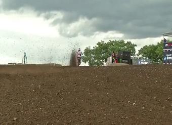
(a) Visual of S.1 in motorcycling.

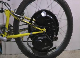
(b) Visual of S.2 in motorcycling.

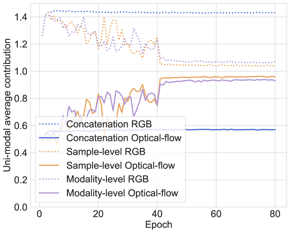
(c) Avg. Contribution on UCF.

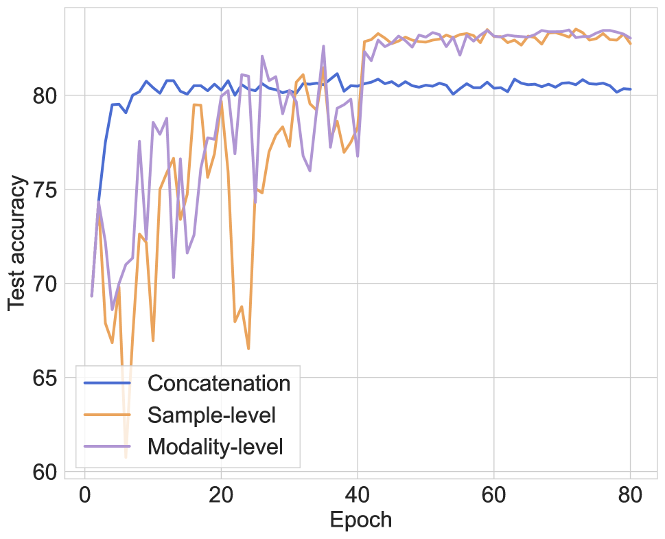
(d) Test Acc on UCF.

Figure 1: (a-b): Audio-visual samples of motorcycling category. (c-d): Average contribution of each modality over all training samples during training and test accuracy of our sample-level and modality-level methods on the UCF-101 (Soomro, Zamir, and Shah 2012) dataset. S.1 and S.2 denotes Sample 1 and Sample 2 respectively. UCF denotes UCF-101. Best viewed in color.

To this end, we introduce a fine-grained modality valuation metric, to observe the contribution of each modality during prediction at the sample-level. The Shapley value in game theory (Shapley 1953), which aims to fairly distribute the benefits based on the contribution of each player, provides the theoretical support of our valuation. This Shapely-based metric could offer a reasonable observation of fine-grained multi-modal cooperation, handling the realistic scenarios where the discrepancy between modalities could vary across samples. By means of valuating uni-modal contribution, we observe that the experiment results unsatisfactorily fail to meet the expectation that each modality has its irreplaceable contribution. In Figure 1(c), we show the average contribution of each modality over all training samples on the UCF-101 dataset. Based on the results (the blue lines), we observe a phenomenon that the contribution of one modality overwhelms others. Then, we further analyze the effect of the modality with clear lower contribution in a sample and find that its presence would potentially increase the risk that the multi-modal model collapses to one specific modality, worsening the cooperation between modalities. Hence, it is urgent to recover the suppressed contribution of the low-contributing modality.

To alleviate the above problem, we analyze the correlation between uni-modal discriminative ability and its contribution, then find that enhancing the discriminative ability of low-contributing modality during training could indirectly improve its contribution in a sample, and accordingly enhance multi-modal cooperation. Therefore, we propose to train the low-contributing modality in a sample with a targeted manner based on the contribution discrepancy between modalities. Specifically, we first valuate the uni-modal contribution at sample-level via our Shapley-based modality valuation metric. Then input of identified low-contributing modalities is re-sampled with dynamical frequency determined by the exact contribution discrepancy, to targetedly improve its discriminative ability. Considering the computational cost of sample-wise modality valuation, we also propose the more efficient modality-wise method.

With our methods, the contribution of overwhelmed modality is recovered to some extent, improving multi-modal cooperation, and model performance is subsequently boosted (orange and purple lines in Figure 1(c) and 1(d)). Overall, our contributions are as follows. Firstly, we introduce a fine-grained modality valuation metric to observe the uni-modal contribution at sample-level. Secondly, we observe and further analyze the low-contributing modality issue, which could worsen the multi-modal cooperation. Thirdly, methods are proposed to strengthen low-contributing modalities, reasonably improving multi-modal cooperation.

2 Related works

2.1 Multi-modal learning

Inspired by humans’ multi-sensory experience, multi-modal learning, aiming to build models that can integrate information from multiple modalities, has raised attention and witnessed rapid development in recent years (Baltrušaitis, Ahuja, and Morency 2018). The research of multi-modal learning covers a wide range of areas, such as multi-modal recognition (Xu, Zhu, and Clifton 2023) and audio-visual scene understanding (Zhu et al. 2021). The widely-used jointly trained multi-modal frameworks often extract and integrate uni-modal features, then optimize all modalities with a uniform learning objective. However, besides the apparent performance, the inherent contribution of different modalities is still under-explored.

2.2 Game theory in machine learning

Game theory is a theoretical framework for conceiving situations among players. All along, researchers have also adapted the game theory to formulate and solve machine learning problems (Freund and Schapire 1996; Wang et al. 2017; Gemp et al. 2020). For example, in the early stage, game theory has been associated with the AdaBoost and used to explain the algorithm effectiveness (Freund and Schapire 1996). More recently, the success of Generative Adversarial Networks is tight with the theoretical foundation of game theory (Wang et al. 2017).

Similarly to us, Hu et al. (Hu, Li, and Zhou 2022) use the Shapley value to evaluate the overall contribution of individual modalities for the whole dataset. However, this study could not capture the modality contribution at sample-level and does not provide analysis or methods for the worse multi-modal cooperation phenomenon. In this paper, we not only explore the fine-grained modality valuation to observe the contribution of each modality at sample-level, but also further analyze the resulting low-contribution issue, accordingly improving multi-modal cooperation.

2.3 Imbalanced multi-modal learning

Multi-modal model is expected to outperform its uni-modal counterpart since it takes more information, but recent studies have found the multi-modal model has a preference for specific modality, limiting its performance (Huang et al. 2022). Several methods have been proposed to ease this problem by improving the uni-modal optimization in the jointly trained multi-modal framework (Wang, Tran, and Feiszli 2020; Peng et al. 2022; Wu et al. 2022). These methods often control uni-modal optimization by estimating the discrepancy of the training stage or performance between modalities. However, their estimation, i.e., the logits or the scale of gradient, often limited to simple fusion methods or could be hard to observe modality discrepancy at sample-level, handling the realistic scenarios where performance difference of each modality could vary across samples. In this paper, we go a step further, reasonably valuating the uni-modal contribution at sample-level using the introduced Shapley-based metric. This fine-grained modality valuation metric with theoretical support could help to observe uni-modal contribution at sample-level, and guide us to solve the imbalanced multi-modal learning problem better.

3 Method

3.1 Model formulation

In this paper, we consider the multi-modal discriminative task. Concretely, each sample $x=(x^{1},x^{2},\cdots,x^{n})$ is with $n$ modalities. And $y$ is the ground truth label of sample $x$. For simplicity, the input of modality $i$ in specific sample $x$ is denoted as modality $x^{i}$. $N=\{x^{1},x^{2},\cdots,x^{n}\}$ is a finite, non-empty set of all modalities. Denote the multi-modal model as $H(\cdot)$. Suppose $\mathcal{C}$ is the set of input modalities for the model. Then, when taking modalities in $\mathcal{C}$ as the model input, the final prediction is $\widehat{y_{C}}=H(\cup x^{i},x^{i}\in\mathcal{C})$. It should be noted that we have no assumption of multi-modal fusion design, therefore the following modality valuation is not limited to simple fusion strategy.

3.2 Fine-grained modality valuation

In multi-modal learning, each modality is expected to fully demonstrate its irreplaceable contribution, since different modalities are considered with complementary information. Especially, recent studies have revealed that the jointly trained multi-modal model often could not utilize all modalities well (Huang et al. 2022). What’s more, based on data samples of realistic scenarios, the modality contribution discrepancy could vary across different samples. Hence, it is necessary to valuate the uni-modal contribution in the multi-modal model at sample-level, and accordingly improve multi-modal cooperation. In this paper, we introduce a Shapely-based metric fine-grained modality valuation metric, to observe the uni-modal contribution for the multi-modal prediction at sample-level.

Concretely, we first have $v$ as a function to map the multi-modal prediction to its benefits:

$$v(\mathcal{C})=\begin{cases}|\mathcal{C}|&\text{ if }\widehat{y_{C}}=y,\\ 0&\text{otherwise}.\end{cases}$$ (1)

When predicting correctly, the benefits of multi-modal prediction with input $\mathcal{C}$ is the number of input modalities.

After formulating the model benefits, to consider the contribution of each modality under all cases, let $\Pi_{N}$ denote the set of all permutations of $N$. For modality $x^{i}$, given a permutation $\pi\in\Pi_{N}$, we denote by $S_{\pi}(x^{i})$ the set of all predecessors of it in $\pi$, i.e., we set $S_{\pi}(x^{i})=\{x^{j}\in N|\pi(x^{j})<\pi(x^{i})\}$. The marginal contribution of $x^{i}$ with respect to a permutation $\pi$ is denoted by $\Delta_{\pi}(x^{i})$ and is given by:

$$\Delta_{\pi}(x^{i})=v(S_{\pi}(x^{i})\cup{x^{i}})-v(S_{\pi}(x^{i})).$$ (2)

This quantity measures how much modality $x^{i}$ increases the benefits of its predecessors in $\pi$ when it joins them. We can now calculate the contribution of $x^{i}$, where the average marginal contribution is taken over all permutations of $N$. Then, given a multi-modal model with $n!$ permutation, the contribution of modality $x^{i}\in N$ is denoted by $\phi^{i}$ and is given by:

$$\phi^{i}=\frac{1}{n!}\sum_{\pi\in\Pi_{N}}\Delta_{\pi}(x^{i}).$$ (3)

It should be noted that when considering all permutations, the sum of uni-modal contribution $\phi^{i}$ is in fact the benefit of multi-modal prediction with all modalities as the input. Hence, for the normal multi-modal model with all modalities as the input, when the contribution of one modality increases, the contribution of other modalities would accordingly decrease. With the aid of this fine-grained modality valuation metric, we could reasonably observe the uni-modal contribution for each sample, preparing for improving multi-modal cooperation.

3.3 Low-contributing modality phenomenon

In Figure 1(c), we show the average contribution of each modality over all training samples on the UCF-101 dataset. However, based on the experiment results, we can observe that the uni-modal average contribution has an obvious preference for specific modality: the contribution of one modality highly overwhelms others. In other words, the decision of multi-modal model is dominated by one modality, remaining others low-contributing.

Corollary 1.

Suppose the marginal contribution of modality is non-negative. For the normal multi-modal model with all modalities of sample $x$ as the input, with benefits $v(N)=n$, when modality $x^{k}$ is low-contributing, i.e., $\phi^{k}<1$, the difference between $v(N)$ and $v(N\backslash x^{k})$ decreases.

Here we analyze the effect of low-contributing modality to the benefits of normal multi-modal model for sample $x$, and have Corollary 1. Based on it, the existence of low-contributing modality results in the benefits of taking all modalities $N$ as the input becomes close to its subset, which means that the multi-modal integration becomes less effective, weakening the cooperation between modalities. Assuming an extreme case where the contribution of all but one modality is very small, multi-modal learning is close to uni-modal learning. Hence, it is essential to enhance the contribution of low-contributing modalities for each sample, improving multi-modal cooperation.

Corollary 2.

Suppose the marginal contribution of modality is non-negative and the numerical benefits of one modality’s marginal contribution follow the discrete uniform distribution. Enhancing the discriminative ability of low-contributing modality $x^{k}$ can increase its contribution $\phi^{k}$.

To alleviate the above problem, we further analyze the correlation between uni-modal discriminative ability and its contribution and have Corollary 2. Based on the analysis, strengthening the discriminative ability of low-contributing modality is able to improve its contribution to multi-modal prediction. Correspondingly, the risk that multi-modal model collapses to one specific modality is lowered.

3.4 Re-sample enhancement strategy

Based on Section 3.3, enhancing the discriminative ability of low-contributing modality can expand its contribution. Hence, we propose to improve the discriminative ability of low-contributing modality during training by a simple strategy that re-sampling its input in a targeted manner. We also want to note that the used re-sample strategy is a tool to enhance discriminative ability (Ando and Huang 2017), and more strategies can be attempted under the guidance of our fine-grained modality valuation and analysis.

Concretely, to ensure the basic discriminative ability, we first warm up the multi-modal model for several epochs. Then, after each epoch, modality valuation is conducted once to observe uni-modal contribution for each sample. Subsequently, learning of the low-contributing modality can be targetedly improved via solely re-sampling its input. Here, we provide the fine-grained as well as effective sample-level re-sample method and the coarse but efficient modality-level re-sample method.

Sample-level re-sample

After the modality valuation, the low-contributing modality, $\phi^{j}<1$, for each sample, can be well distinguished and we can finely improve its learning at sample-level. Then the specific re-sample frequency is dynamically determined by the exact value of $\phi^{j}$ during training. Specifically, the re-sample frequency of modality $x^{j}$ for specific sample $x$ is:

$$s(x^{j})=\left\{\begin{array}[]{cl}f_{s}(1-\phi^{j})&\text{ }\phi^{j}<1,\\ 0&\text{ others, }\end{array}\right.$$ (4)

where $f_{s}(\cdot)$ is a monotonically increasing function. Utilizing this sample-level re-sample strategy, the low-contributing modality in sample $x$ is re-trained with a re-sample frequency inversely proportional to its contribution, i.e., the less the contribution is, the larger the re-sample frequency is. It is worth noting that only the low-contributing modality is taken during re-sampling, and the inputs of other modalities are masked by $0$, to ensure targeted learning.

Modality-level re-sample

Although sample-level modality valuation could provide fine-grained uni-modal contribution, there would be a high additional computational cost when the scale of dataset is quite large. Therefore, the more efficient modality-level method is proposed to lower cost. As Figure 1(c), the low-contributing phenomenon has a modality-level preference. For example, the average contribution of RGB modality over all training samples is obviously more than that of optical flow modality on the UCF-101 dataset. Hence, we propose a more coarse modality-level re-sample strategy, which estimates the average uni-modal contribution via only conducting modality valuation on the subset of training samples to reduce additional computational cost.

Concretely, we randomly split a subset with $Z$ samples in the training set to approximately estimate the average uni-modal contribution. Hence, the overall low-contributing modality $x^{k}$ with less $\phi^{k}$ can be approximately identified. Then, other modalities remain unchanged, and modality $x^{k}$ in sample $x$ is dynamically re-sampled with specific probability during training via:

$$p(x^{k})=f_{m}(\text{Norm}(d)),$$ (5)

where $d=\frac{1}{n-1}(\sum^{n}_{j=1,j\neq k}(\frac{\sum^{Z}_{i=1}\phi_{i}^{j}}{Z}-\frac{\sum^{Z}_{i=1}\phi_{i}^{k}}{Z}))$. The discrepancy in average contribution between overall low-contributing modality $x^{k}$ compared to others (i.e., $d$) is first $0-1$ normalized, then fed into $f_{m}(\cdot)$, a monotonically increasing function with a value between $0$ and $1$. $n$ is the number of modalities. The re-sample probability for overall low-contributing modality $x^{k}$ is proportional to the discrepancy in its average contribution compared to others. Compared to sample-level strategy, modality-level strategy is more efficient by utilizing the modality preference of the dataset.

4 Experiment

4.1 Dataset and experimental settings

Kinetics Sounds (KS) (Arandjelovic and Zisserman 2017) is an action recognition dataset containing 31 human action classes selected from Kinetics dataset (Kay et al. 2017). All videos are 10 seconds. This dataset contains 19k video clips.

UCF-101 (Soomro, Zamir, and Shah 2012) is an action recognition dataset of realistic action videos with two modalities: RGB and optical flow. It has 13,320 videos from 101 action categories.

MM-Debiased is an audio-visual dataset proposed in this work, where modality-level low-contributing preference is not obvious. It covers 10 classes, and contains 11,368 training samples and 1,472 testing samples. Details about the dataset construction are provided in Supp. Materials.

Experimental settings. Encoders used for UCF-101 are ImageNet pre-trained, and others are trained from scratch. A subset with $20\%$ training samples is randomly split in modality-level method. During modality valuation, for input modality set $\mathcal{C}$, input of modalities not in $\mathcal{C}$ are zeroed out, similar to related work (Ghorbani and Zou 2020). During testing, all modalities are taken as the model input. Detailed experimental settings, experiments about more than two modalities, and ablation studies about the subset scale, $f_{s}(\cdot)$ as well as $f_{m}(\cdot)$, are provided in Supp. Materials.

4.2 Comparison with multi-modal models

Here we first compare our methods with several representative multi-modal deep frameworks: Concatenation (Owens and Efros 2018), Summation, and Decision fusion (Simonyan and Zisserman 2014). Two specifically-designed fusion methods Film (Perez et al. 2018) and Gated (Kiela et al. 2018) are also compared. In addition, the early multi-modal integration attempts, Bayesian network (Blundell et al. 2015) and Multi-kernel Learning (MKL) (Sikka et al. 2013), are also compared. To be fair, the uni-modal encoders of Bayesian network are ResNet-18 and features fed into MKL are extracted by pre-trained uni-modal encoders. Our sample-level and modality-level methods are based on Concatenation fusion in Table 1. What’s more, since the utilized re-sample strategy increases training efforts, we compare two related re-sample settings to validate the effectiveness of ours, naïve re-sample and reversed re-sample. The naïve re-sample is to randomly re-sample input of each modality with the same frequency as ours, while the reversed re-sample is contrary to our methods, only re-sampling the data of modality with higher contribution. Based on Table 1, several observations can be revealed.

Method	KS		UCF-101
	(Audio+Visual)		(RGB+OF)
	Acc	mAP	Acc	mAP
Concatenation	62.30	67.95	81.15	86.15
Summation	62.10	66.97	81.31	86.25
Decision fusion	62.65	67.89	79.81	86.07
Film	61.25	64.85	79.45	84.27
Gated	62.72	68.28	81.34	86.35
Bayesian DNN	60.79	64.98	80.04	84.95
Deep MKL*	63.61	69.69	82.64	87.96
Naïve re-sample	64.69	70.87	82.56	88.02
Reversed re-sample	59.03	63.14	80.85	85.06
Sample-level	66.92	71.84	83.52	88.89
Modality-level	66.65	72.68	83.46	88.75

Table 1: Comparison with different multi-modal models. * denotes that the fed feature of Deep MKL model is extracted by pre-trained uni-modal encoders. Bayesian DNN is trained from scratch. OF denotes for optical flow.

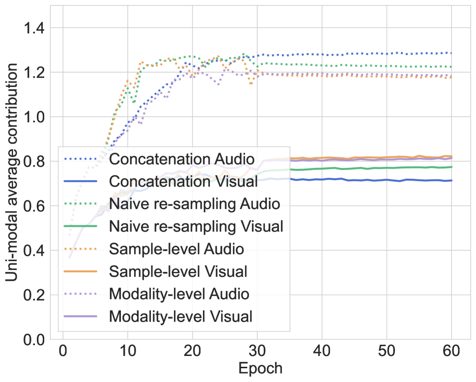
(a) Naïve comparison.

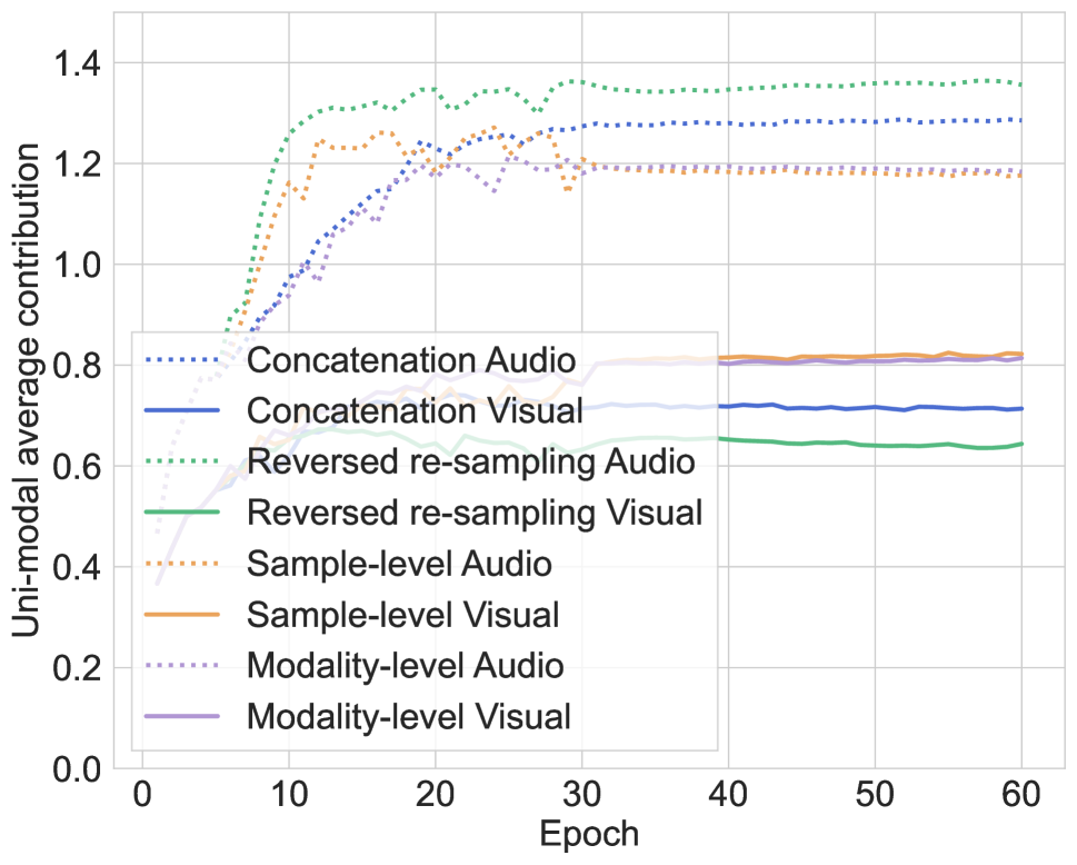
(b) Reversed comparison.

Figure 2: Average contribution of each modality over all training samples during training for Naïve re-sample and Reversed re-sample methods on the Kinetics Sounds dataset.

Firstly, the traditional multi-modal learning methods are able to disclose their effectiveness after being equipped with extracted deep features, especially MKL, which even outperforms the Concatenation model. However, this improvement has a reliance on the quality of input features, and these methods are still hard to directly process raw data in large-scale. Secondly, both our sample-level and modality-level strategies improve multi-modal cooperation by means of fine-grained modality valuation, achieving better model performance. Moreover, the fine-grained sample-level method tends to be superior. In contrast, the modality-level method is more efficient and sometimes even can be comparable to sample-level one. Thirdly, the naïve re-sample method can also increase model ability. The reason could be that this random uni-modal re-sample setting also potentially provides the chance for each modality to be trained individually, improving the discriminative ability of low-contributing modality. Therefore, the multi-modal cooperation is accordingly boosted based on Corollary 2. As the average uni-modal contribution shown in Figure 2(a), the naïve re-sample method indeed alleviates the low-contributing issues to some extent (the green line). Beyond that, our methods with targeted re-sample design under the guidance of fine-grained modality valuation during training, take one step further (as the orange and purple lines). In addition, the failure of reversed re-sample setting (the green line in Figure 2(b)), which runs counter to our analysis, also validates that it is our modality valuation guidance that matters, rather than the re-sample strategy itself, and other discriminative ability enhancement strategies can also be attempted.

Method	KS	UCF-101	MM-Debiased
Concatenation	62.30	81.15	83.70
Concat-Sample	66.92	83.52	84.58
Concat-Modality	66.65	83.46	84.04
CentralNet	67.35	83.97	85.23
CentralNet-Sample	67.89	84.07	85.39
CentralNet-Modality	68.31	84.05	85.26
MMTM	64.23	80.67	84.31
MMTM-Sample	64.40	81.30	85.33
MMTM-Modality	64.34	81.23	84.71
MBT	47.02	-	68.01
MBT-Sample	47.53	-	68.70
MBT-Modality	47.36	-	68.34

Table 2: Accuracy of multi-modal frameworks with cross-modal interaction modules. Results of MBT on UCF-101 dataset could not be obtained since the lack of suitable pre-trained transformer backbone.

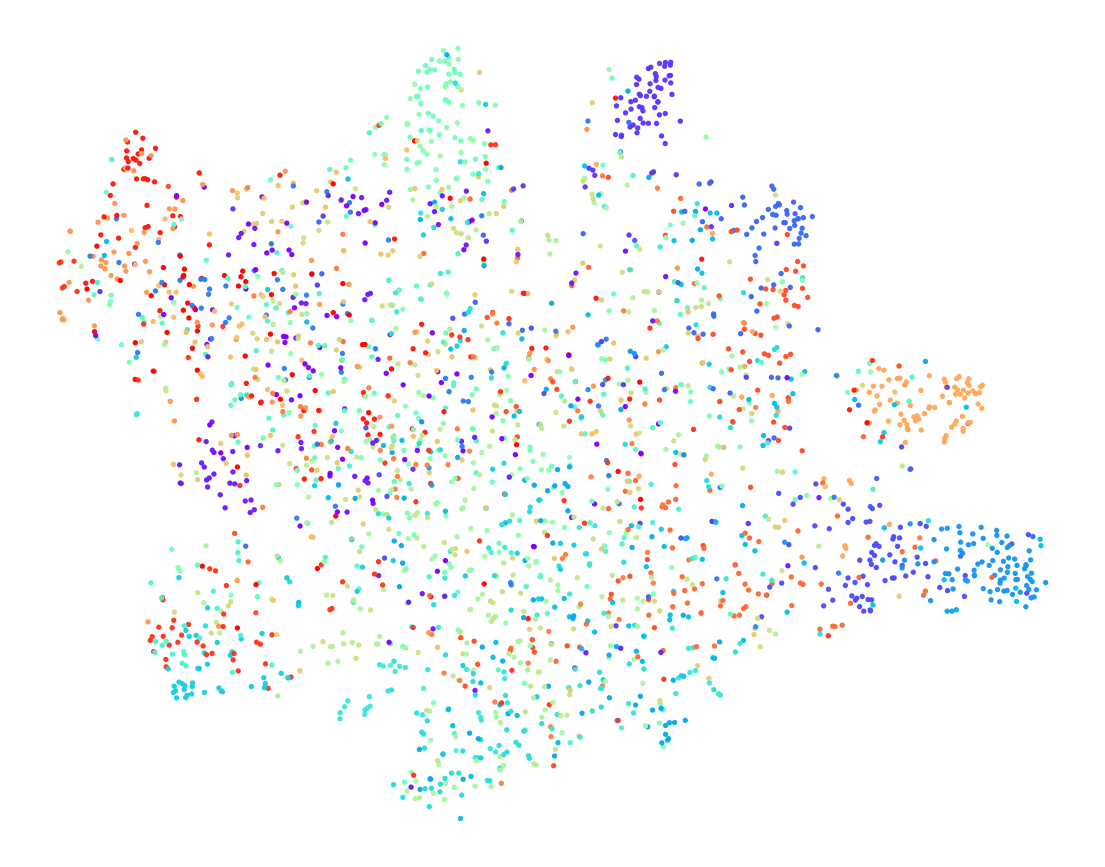
(a) Concatenation.

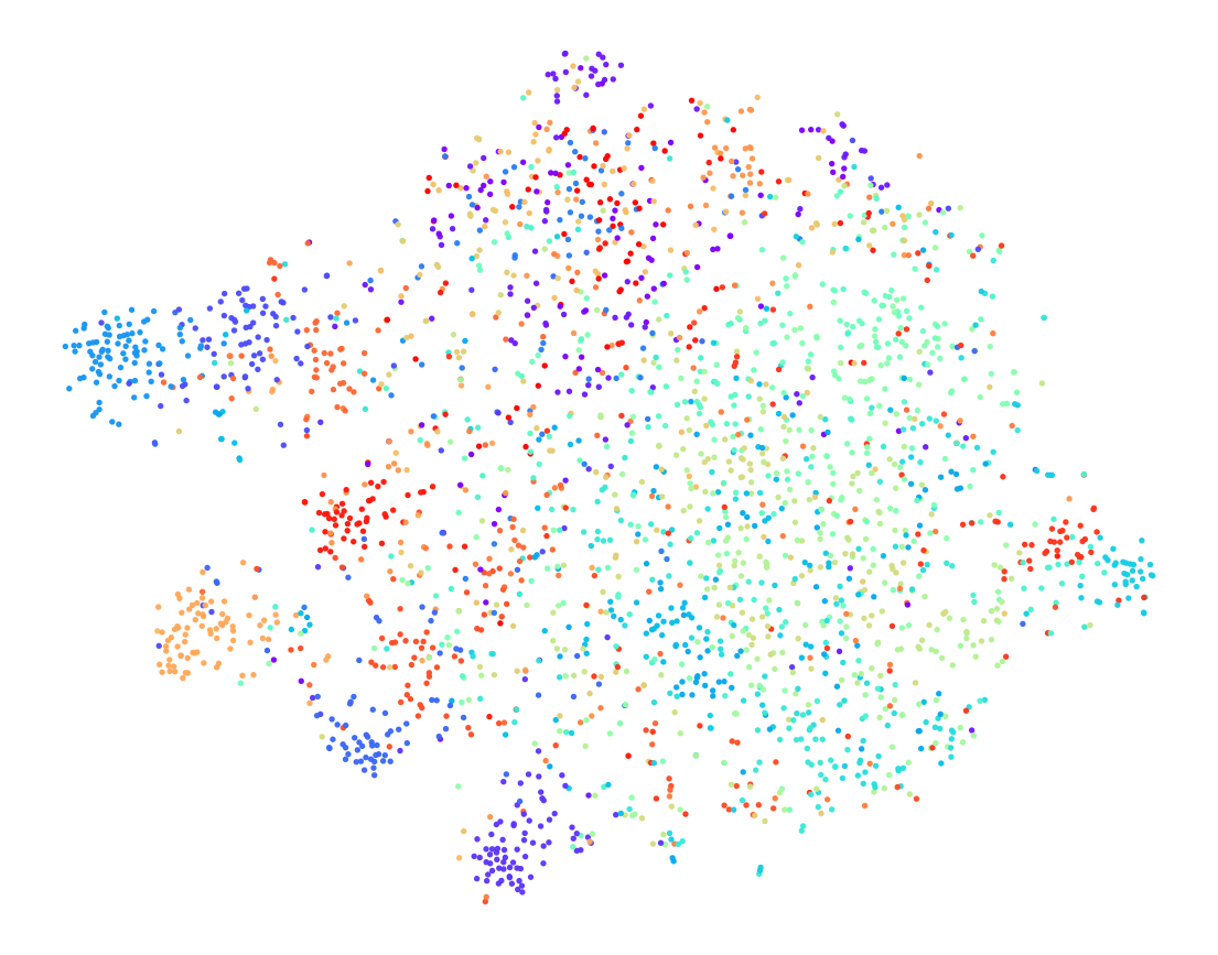
(b) MMTM.

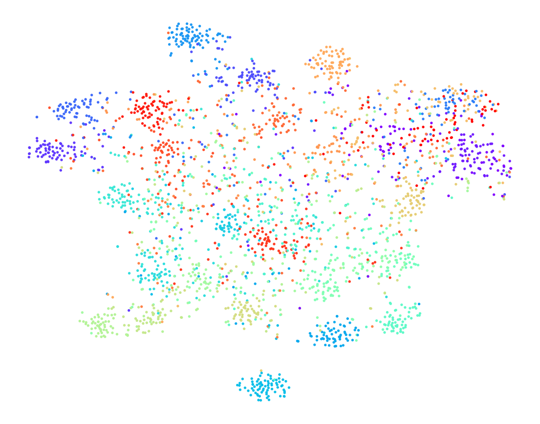
(c) MMTM-Sample.

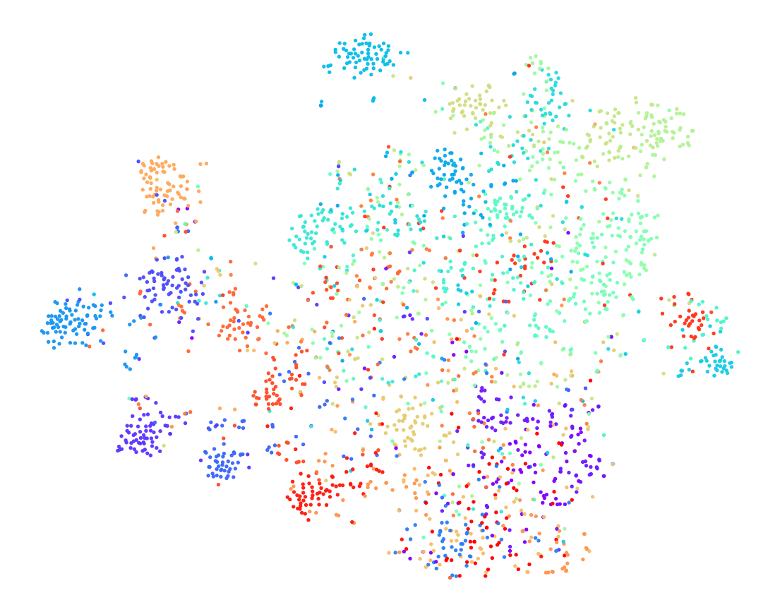
(d) MMTM-Modality.

Figure 3: Visual feature distribution of Concatenation, MMTM, MMTM-Sample and MMTM-Modality, visualized by t-SNE (Van der Maaten and Hinton 2008) on Kinetics Sounds (KS) dataset. Visual modality tends to be the low-contributing modality for samples in KS dataset. The categories are indicated in different colors.

4.3 Cross-modal interaction scenarios

In multi-modal learning, besides simple fusion methods, various cross-modal interaction modules are proposed to improve the integration of different modalities. Here we first combine our sample-level and modality-level methods with two intermediate fusion, CentralNet (Vielzeuf et al. 2018) and MMTM (Joze et al. 2020), to evaluate their effectiveness under these cross-modal interaction scenarios. To be fair, ResNet-18 is also used as the uni-modal backbone. Based on Table 2, these cross-modal interaction modules indeed improve the model performance, compared with Concatenation baseline. This phenomenon demonstrates that the cross-modal interaction could implicitly deepen the cooperation between modalities by helping one modality make adjustments according to the feedback from others. Concretely, CentralNet fused the uni-modal feature of intermediate layer via a learned weighted sum, and MMTM activates the intermediate features of one modality with the guidance of others via the squeeze and excitation module, which can be regarded as self-attention on channels.

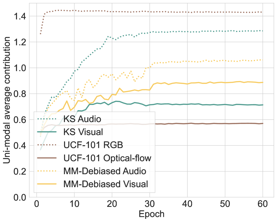
(a) Avg. Contribution of dataset.

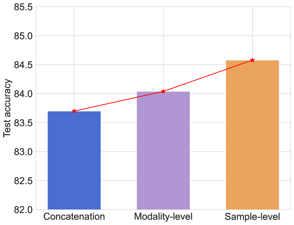
(b) Test Acc on MM-Debiased.

Figure 4: (a) Uni-modal average contribution over all training samples, which is calculated based on the concatenation framework. (b) Test accuracy on the MM-Debiased dataset.

In addition, both our sample-level and modality-level strategies are able to be applied to these more complex scenarios with cross-modal interaction, bringing performance improvement. One additional observation is that although the architecture limits model performance, our method applied to simple Concatenation fusion method could even have comparable results with more complex model designs, indicating it is simple-yet-effective. In addition, to qualitatively observe the quality of uni-modal representations, we visualize the feature distribution of overall low-contributing modality encoder on the Kinetics Sounds dataset (i.e., the visual modality). Results in Figure 3 illustrate that the feature distribution is more discriminative in terms of action categories with cross-modal interaction, and this discriminative distribution can go a step further after being equipped with our methods.

Besides these modules based on CNN backbone, transformer networks also have cross-modal interaction. Here we combine our methods with the representative transformer model, MBT (Nagrani et al. 2021), to explore their effectiveness. Results are shown in Table 2. It should be noted that performance of MBT is inferior to Concatenation with CNN backbone, since the transformer network is generally data-hungry, limiting its performance on these datasets without large enough samples. But both our sample-level and modality-level methods can combine with and further enhance the performance of MBT. Overall, our methods could be well equipped with different cross-modal interaction modules, bringing performance enhancement.

4.4 Fine-grained modality discrepancy scenarios

Considering that conducting modality valuation at the sample-level needs additional computational cost, the modality-level method is proposed to estimate uni-modal contribution discrepancy via the subset of training samples. This method relies on the observation that the low-contributing phenomenon has an overall bias at the modality-level for the curated dataset. Based on the results in Table 1, the modality-level method could achieve considerable performance at a lower cost. To further explore the effectiveness of our methods under the fine-grained modality discrepancy scenarios, we build the MM-Debiased dataset where the modality-level preference is no longer significant. According to the results shown in Figure 4(a), the average contribution of each modality on the MM-Debiased dataset is more balanced than that on other curated datasets.

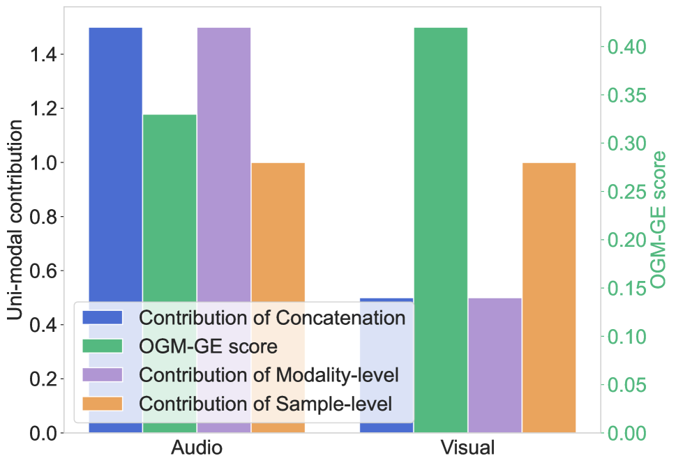
(a) Valuation of Sample 1.

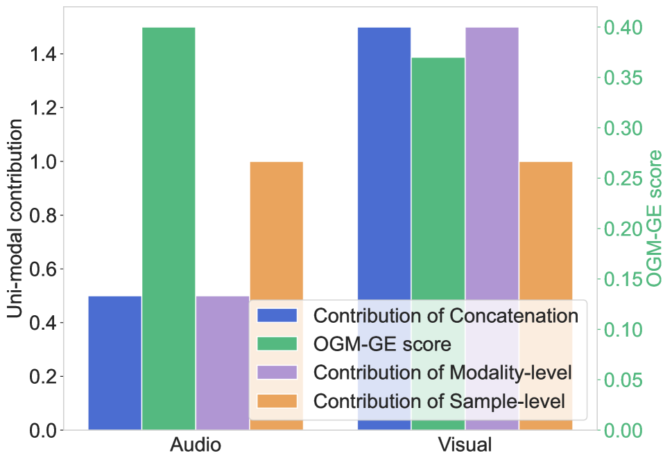
(b) Valuation of Sample 2.

Figure 5: Valuation of two samples of motorcycling category in testing set of the MM-Debiased dataset.

As the results in Figure 4(b) (more in Table 2), the sample-level method has a more obvious advantage than modality-level one on MM-Debiased dataset, since the modality-level preference is no longer reliable, but the low-contributing modality issue still exists at the sample-level. And the contribution discrepancy between modalities could vary across samples. Take two testing samples of motorcycling category in Figure 1(a) and 1(b) as an example. The motorcycle in Sample 1 appears hard to be observed, while the wheel of motorcycle in Sample 2 appears clearly. As shown in Figure 5, the Concatenation model receptively relies on audio or visual signals for these two samples. Not surprisingly, the modality-level method fails to capture and ease this discrepancy. But the fine-grained sample-level strategy could observe it and accordingly adjust the uni-modal learning. Especially, for Sample 1, the softmax confidence for the correct category of modality-level method is only $0.67$ (comparable with Concatenation baseline), while the sample-level method has a greatly higher score of $0.98$. Overall, the sample-level and modality-level methods have their own advantages and applicable scenarios.

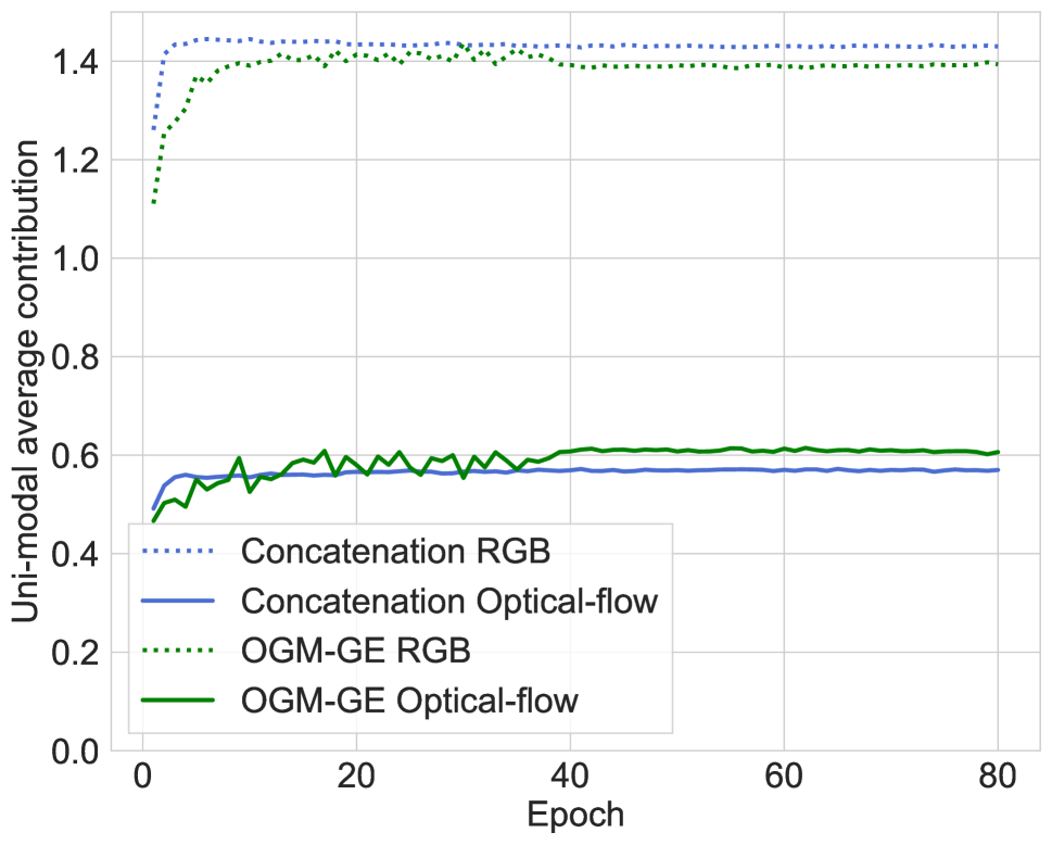
(a) OGM-GE.

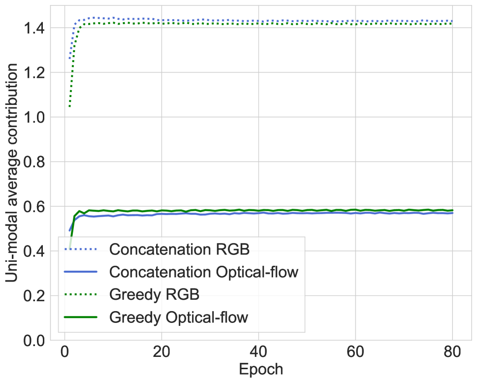
(b) Greedy.

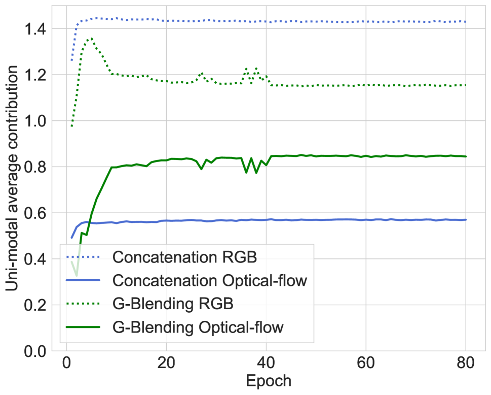
(c) G-Blending.

(d) Ours.

Figure 6: Average contribution of each modality over all training samples during training for OGM-GE, Greedy, G-Blending and our methods on the UCF-101 dataset.

4.5 Comparison with uni-modal modulation methods

Recent studies have found that multi-modal models often cannot jointly utilize all modalities well, and some uni-modal modulation methods are proposed. In this section, we compare these uni-modal modulation methods, G-Blending (Wang, Tran, and Feiszli 2020), OGM-GE (Peng et al. 2022) and Greedy (Wu et al. 2022). They often control uni-modal optimization by estimating the discrepancy of the training stage or performance between modalities. Our sample-level and modality-level methods are based on Concatenation fusion in Table 3. As Table 3, our methods outperform these modulation approaches. Although G-Blending (Wang, Tran, and Feiszli 2020) achieves considerable performance, it needs to train an additional uni-modal classifier as the basis of modulation. In contrast, our modality valuation could directly capture the inherent multi-modal cooperation state without introducing additional uni-modal modules, making it more efficient. Concretely, FLOPs of our methods reduce $1/4$ (sample-level method), even $1/2$ (modality-level method), compared to G-Blending. In addition, since our modality valuation is not limited to specific methods, the uni-modal contribution of other methods can also be observed. As Figure 6, our methods exhibit superior mitigation of imbalanced uni-modal contributions, thereby highlighting our efficacy beyond mere final prediction.

Moreover, to modulate the uni-modal optimization, these methods also evaluate specific uni-modal properties. G-Blending (Wang, Tran, and Feiszli 2020) and Greedy (Wu et al. 2022) inspect the uni-modal training process. But they could not be used to evaluate the modal preference at the sample-level. The uni-modal confidence score used by OGM-GE (Peng et al. 2022) could evaluate uni-modal performance at sample-level. However, this empirically designed score is hard to handle in realistic scenarios, like dominant modality could differ among samples within the same category, since its calculation could suffer from the modality-level preference. For example, in Figure 5, two testing samples of motorcycling category in the MM-Debiased dataset rely on audio and visual signals, respectively. OGM-GE score provides biased valuation results, even assigning more confidence for the less informative visual signal of Sample 1 (the green bar in Figure 5(a)). But our fine-grained modality valuation method could clearly capture this discrepancy (the blue bar in Figure 5(a)), and mitigate this issue by the fine-grained sample-level strategy, as discussed in Section 4.4.

Method	Extra	Total	Accuracy
	Modules	FLOPs*	KS	UCF-101
Concatenation	Baseline	$1.00\times$	62.30	81.15
OGM-GE	✗	$1.00\times$	63.30	81.54
OGM-GE†	✗	$1.00\times$	63.65	82.04
G-Blending	✓	$3.00\times$	66.24	83.09
G-Blending†	✓	$4.00\times$	66.85	83.26
Greedy	✓	$1.01\times$	62.37	81.25
Greedy†	✓	$1.01\times$	62.48	81.41
Sample-level	✗	$2.28\times$	66.92	83.52
Modality-level	✗	$1.44\times$	66.65	83.46

Table 3: Comparison with uni-modal modulation methods. * denotes that the FLOPs is calculated based on Kinetics Sounds. † indicates our modality valuation and analysis are applied. Details are provided in the Supp. Materials.

To further validate the effectiveness of our modality valuation and analysis, we further retain the core modulation settings in these methods (like mitigating gradient in OGM-GE), but with the guidance of our analysis about low-contributing modality. Details are provided in the Supp. Materials. As Table 3, our modality valuation and analysis could further boost their performance, indicating the effectiveness of our observation for uni-modal contribution. Besides, even under the same modality valuation strategy, our methods are still superior to the other boosted modulation methods (OGM-GE†, Greedy†, and G-Blending†), in most cases. This indicates that our modulation method based on targeted analysis is both reasonable and effective.

5 Discussion

In this paper, we introduce a fine-grained modality valuation metric to observe uni-modal contribution with the aid of theory in game theory. Two methods are proposed to recover the suppressed contribution of low-contributing modality, improving multi-modal cooperation. In our experiments, the uni-modal contribution is often not equal to $1$ even after enhancement, as Figure 1(c). The reason could be that there is a natural difference in the discriminative ability of modalities. For example, for an audio-visual sample drawing picture, vision is naturally more discriminative than auditory. Hence, our methods could recover the suppressed contribution of low-contributing modality, but could not make the uni-modal contribution equal. Overall, we reasonably observe the uni-modal contribution and achieve considerable improvement on different multi-modal models.

Appendix A Low-contributing modality phenomenon

Here we consider the multi-modal discriminative task. Concretely, each sample $x=(x^{1},x^{2},\cdots,x^{n})$ is with $n$ modalities. And $y$ is the ground truth label of sample $x$. For simplicity, the input of modality $i$ in specific sample $x$ is denoted as modality $x^{i}$. $N=\{x^{1},x^{2},\cdots,x^{n}\}$ is a finite, non-empty set of all modalities. Denote the multi-modal model as $H(\cdot)$. Suppose $\mathcal{C}$ is the set of input modalities for the model. Then, when taking modalities in $\mathcal{C}$ as the model input, the final prediction is $\widehat{y_{C}}=H(\cup x^{i},x^{i}\in\mathcal{C})$. Then we have $v$ as a function to map the multi-modal prediction to its benefits:

$$v(\mathcal{C})=\begin{cases}|\mathcal{C}|&\text{ if }\widehat{y_{C}}=y,\\ 0&\text{otherwise}.\end{cases}$$

When predicting correctly, the benefits of multi-modal prediction with input $\mathcal{C}$ is the number of input modalities. The contribution of modality $x^{i}\in N$ is calculated based on benefits and denoted by $\phi^{i}$.

A.1 Low-contributing modality issue

Corollary 1.

Suppose the marginal contribution of modality is non-negative. For the normal multi-modal model with all modalities of sample $x$ as the input, with benefits $v(N)=n$, when modality $x^{k}$ is low-contributing, i.e., $\phi^{k}<1$, the difference between $v(N)$ and $v(N\backslash x^{k})$ decreases.

Proof.

Suppose the marginal contribution of modality in multi-modal learning is non-negative, since the introduction of additional modality tends to not bring negative effects in practice. Based on the definition of uni-modal contribution for modality $x^{k}$, we have:

$$\phi^{k}=\frac{1}{n!}\sum_{\pi\in\Pi_{N}}\Delta_{\pi}(x^{k}),$$ (6)

$$\phi^{k}=\frac{1}{n!}\sum_{\pi\in\Pi_{N}}(v(S_{\pi}(x^{k})\cup{x^{k}})-v(S_{\pi}(x^{k}))),$$ (7)

$$n!\cdot\phi^{k}\geq(n-1)!\cdot(\underbrace{v(N)-v(N\backslash x^{k})}_{\text{only consider cases $x^{k}$ is the last one}}),$$ (8)

$$n\cdot\phi^{k}\geq v(N)-v(N\backslash x^{k}),$$ (9)

$$v(N)-v(N\backslash x^{k})\leq n\cdot\phi^{k}.$$ (10)

In addition, based on the definition of function $v$, when predicting correctly, $v(N)=n$, and the minimum of $v(N\backslash x^{k})$ is $0$. Then we have:

$$v(N)-v(N\backslash x^{k})\leq n.$$ (11)

However, based on Equation 10, when $\phi^{k}<1$, the upper bound of the difference between $v(N)$ and $v(N\backslash x^{k})$ shrinks (i.e., $n\cdot\phi^{k}<n$). In other words, when the contribution of modality $x^{k}$, $\phi^{k}<1$, the benefits of taking all modalities $N$ as the input becomes close to its subset. The difference between $v(N)$ and $v(N\backslash x^{k})$ decreases.

∎

Based on the above analysis, the existence of low-contributing modality ($\phi^{k}<1$) leads to the benefits degradation of normal multi-modal model with all modalities of sample $x$ as the input. Assuming an extreme case where the contribution of all but one modality is very small, multi-modal learning collapses to specific modality.

In Corollary 1, we consider the low-contributing modality for $v(N)=n$, i.e., for correct prediction. As for the situation $v(N)=0$, i.e., the multi-modal model provide wrong prediction, it could be caused by more fundamental reasons, like limited model capacity or outlier sample, beyond the low-contributing issue.

In addition, here we suppose the marginal contribution of modality is non-negative. In practice, the introduction of additional modalities has been validated its benefit (non-negative effect) across different application tasks (liang2022foundations). It also theoretically proves that multi-modal learning provably performs better than uni-modal (huang2021makes). These evidences indicate that the introduction of another related modality could not bring a negative impact in most cases. Based on this, we assume that the marginal contribution is non-negative.

A.2 Low-contributing modality enhancement

Corollary 2.

Suppose the marginal contribution of modality is non-negative and the numerical benefits of one modality’s marginal contribution follow the discrete uniform distribution. Enhancing the discriminative ability of low-contributing modality $x^{k}$ can increase its contribution $\phi^{k}$.

Proof.

Denote after discriminative ability enhancement, the benefits that only having modality $x^{k}$ as model input is $v^{\prime}(\{x^{k}\})$. And the contribution after enhancement is $\phi^{\prime k}$. The marginal contribution of $x^{k}$ after enhancement with respect to a permutation $\pi$ is denoted by $\Delta_{\pi}^{\prime}(x^{k})$. $N=\{x^{1},x^{2},\cdots,x^{n}\}$ is a finite, non-empty set of modalities. $n$ is the number of modalities. $S_{\pi}(x^{k})$ denotes the set of all predecessors of modality $x^{k}$ in $\pi$.

When $x^{k}$ is the first one in the permutation, $v(\{x^{k}\})$ is the marginal contribution of $x^{k}$. Based on the definition of function $v$, benefits reflects the discriminative ability, then the benefits that only having modality $x^{k}$ as model input would accordingly increase after enhancing its discriminative ability:

$$v^{\prime}(\{x^{k}\})-v(\{x^{k}\})>0.$$ (12)

When $x^{k}$ is not the first one in the permutation, for a specific permutation $\pi$, suppose the marginal contribution of modality is non-negative, since the introduction of additional modality tends to not bring negative effects in practice. Denote $S_{\pi}(x^{k})$ has $c-1$ modalities. Then, based on the definition of function $v$, $\Delta_{\pi}(x^{k})$ can be $0$ ($v(S_{\pi}(x^{k})\cup{x^{k}})=v(S_{\pi}(x^{k}))$), $1$ ($v(S_{\pi}(x^{k})\cup{x^{k}})=c,v(S_{\pi}(x^{k}))=c-1$), and $c$ ($v(S_{\pi}(x^{k})\cup{x^{k}})=c,v(S_{\pi}(x^{k}))=0$).

Suppose the numerical value of one modality’s marginal contribution follows the discrete uniform distribution, then $\Delta_{\pi}^{\prime}(x^{k})-\Delta_{\pi}(x^{k})$ have following cases with equal probability:

(1) $\Delta_{\pi}^{\prime}(x^{k})=\Delta_{\pi}(x^{k})=0$. $\Delta_{\pi}^{\prime}(x^{k})-\Delta_{\pi}(x^{k})=0$.

(2) $\Delta_{\pi}^{\prime}(x^{k})=0$, $\Delta_{\pi}(x^{k})=1$. $\Delta_{\pi}^{\prime}(x^{k})-\Delta_{\pi}(x^{k})=-1$.

(3) $\Delta_{\pi}^{\prime}(x^{k})=0$, $\Delta_{\pi}(x^{k})=c$. $\Delta_{\pi}^{\prime}(x^{k})-\Delta_{\pi}(x^{k})=-c$.

(4) $\Delta_{\pi}^{\prime}(x^{k})=\Delta_{\pi}(x^{k})=1$. $\Delta_{\pi}^{\prime}(x^{k})-\Delta_{\pi}(x^{k})=0$.

(5) $\Delta_{\pi}^{\prime}(x^{k})=1$, $\Delta_{\pi}(x^{k})=0$. $\Delta_{\pi}^{\prime}(x^{k})-\Delta_{\pi}(x^{k})=1$.

(6) $\Delta_{\pi}^{\prime}(x^{k})=1$, $\Delta_{\pi}(x^{k})=c$. $\Delta_{\pi}^{\prime}(x^{k})-\Delta_{\pi}(x^{k})=1-c$.

(7) $\Delta_{\pi}^{\prime}(x^{k})=\Delta_{\pi}(x^{k})=c$. $\Delta_{\pi}^{\prime}(x^{k})-\Delta_{\pi}(x^{k})=0$.

(8) $\Delta_{\pi}^{\prime}(x^{k})=c$, $\Delta_{\pi}(x^{k})=0$. $\Delta_{\pi}^{\prime}(x^{k})-\Delta_{\pi}(x^{k})=c$.

(9) $\Delta_{\pi}^{\prime}(x^{k})=c$, $\Delta_{\pi}(x^{k})=1$. $\Delta_{\pi}^{\prime}(x^{k})-\Delta_{\pi}(x^{k})=c-1$.

Based on the assumption, all cases are with equal probability, then, for a specific permutation $\pi$ (except the modality $x^{k}$ is the first one):

$$\mathbb{E}(\Delta_{\pi}^{\prime}(x^{k})-\Delta_{\pi}(x^{k}))=0.$$ (13)

Combined Equation 12 and Equation 13, we have,

$$\mathbb{E}(\phi^{\prime k}-\phi^{k})=\mathbb{E}(\frac{1}{n!}\sum_{\pi\in\Pi_{N}}\Delta_{\pi}^{\prime}(x^{k})-\frac{1}{n!}\sum_{\pi\in\Pi_{N}}\Delta_{\pi}(x^{k})),$$ (14)

$$\mathbb{E}(\phi^{\prime k}-\phi^{k})=\mathbb{E}(\frac{1}{n!}\sum_{\pi\in\Pi_{N}}(\Delta_{\pi}^{\prime}(x^{k})-\Delta_{\pi}(x^{k}))),$$ (15)

$$\mathbb{E}(\phi^{\prime k}-\phi^{k})=\mathbb{E}(\underbrace{\frac{(n-1)!}{n!}(v^{\prime}(\{x^{k}\})-v(\{x^{k}\}))}_{\text{only cases $x^{i}$ is the first one, which have $(n-1)!$ permutation}}),$$ (16)

$$\mathbb{E}(\phi^{\prime k}-\phi^{k})>0.$$ (17)

Then, we can have enhancing the discriminative ability of low-contributing modality $x^{k}$ can increase its contribution in the multi-modal learning.

∎

Appendix B Experimental settings

When not specified, ResNet-18 (He et al. 2016) is used as the backbone in experiments. Concretely, for the visual encoder, we take multiple frames as the input, and feed them into the 2D network like (Zhao et al. 2018) does; for the audio encoder, we modified the input channel of ResNet-18 from three to one like (Chen et al. 2020) does and the rest parts remain unchanged; for the optical flow encoder, we stack the horizontal vector $u$ and vertical vector $v$ in the way of $[u,v]$ to form as one frame, then multiple frames are also put into the ResNet-18 as (Zhao et al. 2018) does; for the text data, the pre-trained BERT (Devlin et al. 2018) is used to extract embeddings. Encoders used for UCF-101 are ImageNet pre-trained. Encoders of other datasets are trained from scratch.

Videos are extracted frames with 1fps and three frames are uniformly sampled as the visual input. Three optical flow frames are also uniformly sampled in each video. Audio of Kinetics Sounds is converted to a $128\times 1024$ spectrogram with 128-dim log-mel filterbank and a 25ms Hamming window. The audio data of MM-Debiased dataset is transformed into a spectrogram with size $257\times 1,003$ using a window with length of 512 and overlap of 353.

During the training, we use SGD with momentum ($0.9$) and set the learning rate at $1e-3$. All models are trained on 2 NVIDIA RTX 3090 (Ti). In experiments, we randomly split a subset with $20\%$ training samples for the average uni-modal contribution estimation in the modality-level method. During modality valuation, for input modality set $\mathcal{C}$, input of modalities not in $\mathcal{C}$ are zeroed out, similar to related work (Ghorbani and Zou 2020). During testing, all modalities are taken as the model input.

Appendix C Construction of MM-Debiased dataset

To evaluate our proposed methods on the dataset with less modality preference of low-contributing phenomenon, we construct the MM-Debiased dataset. We first train uni-modal ResNet-18 model on the audio and visual modality of VGG-Sound (Chen et al. 2020) and Kinetics-400 dataset (Kay et al. 2017). During training, we record the mean uni-modal softmax scores of each training and testing sample, which reflects the confidence for the sample (Neumann, Zisserman, and Vedaldi 2018). Then, we select the training samples of 10 classes that have a close summation of uni-modal softmax scores on both modalities from the two datasets. The testing samples are then selected from the 10 classes with the same strategy. The selected 10 classes are playing piano, playing cello, lawn mowing, singing, cleaning floor, bowling, whistling, motorcycling, playing flute and writing on blackboard. Based on the result in Figure 4a of the manuscript, the average contribution of each modality over all training samples during training on MM-Debiased is apparently closer than Kinetics Sounds and UCF-101.

Appendix D Combination with modulation methods

To introduce our modality valuation metric and analysis into the existing uni-modal modulation methods, we make some modifications to them. Suppose that dataset has two modalities $u$ and $v$. During modulation, we calculate the gap between the uni-modal contribution and $1$ ( $\phi^{k}<1$, modality $x^{k}$ is low-contributing, based on Corollary 1) for the modality $x^{u}$ and $x^{v}$. Then, this gap is marked as $g^{u}$ and $g^{v}$ for specific sample $x$, where $s$ is the uni-modal contribution:

$$\begin{split}g^{u}=1-s^{u},\\ g^{v}=1-s^{v}.\end{split}$$ (18)

For OGM-GE (Peng et al. 2022), we hope to mitigate the gradients of the modality with higher contribution and slightly boost the gradients of the modality with a lower contribution to balance modality contribution discrepancy. The calculation of gradient coefficients $k_{t}^{u}$ and $k_{t}^{v}$ in iteration $t$ is associate with the average $g^{u}$ and $g^{v}$ within mini-batch:

$$\begin{split}k_{t}^{u}=\begin{cases}1+tanh(\alpha^{ogm}\cdot\beta\cdot\overline{g^{u}_{t}})&\text{ if }\overline{g^{u}_{t}}>0,\\ 1+tanh(\alpha^{ogm}\cdot\overline{g^{u}_{t}})&\text{otherwise},\end{cases}\\ k_{t}^{v}=\begin{cases}1+tanh(\alpha^{ogm}\cdot\beta\cdot\overline{g^{v}_{t}})&\text{ if }\overline{g^{v}_{t}}>0,\\ 1+tanh(\alpha^{ogm}\cdot\overline{g^{v}_{t}})&\text{otherwise},\end{cases}\end{split}$$ (19)

where $k_{t}^{u}$ and $k_{t}^{v}$ are coefficients of gradients to the corresponding uni-modal encoder of each modality, $\overline{g^{u}_{t}}$ and $\overline{g^{v}_{t}}$ are gaps between the average uni-modal contribution and $1$ within the mini-batch, and $\alpha^{ogm}$ is a hyper-parameter in OGM-GE to control the strength of modulation. $\beta$ is a small positive value to limit the increase of gradient of modality with a greater contribution.

For G-Blending (Wang, Tran, and Feiszli 2020), we first compute the weight of multi-modal loss $w^{uv}$ in the same way as the original online G-Blending and fix the summation of the weight of uni-modal losses $w^{u}+w^{v}=1-w^{uv}$. Then, we determine the value of $w^{u}$ and $w^{v}$ through gaps between the average uni-modal contribution and $1$ on the whole dataset $\overline{g^{u}_{d}}$ and $\overline{g^{v}_{d}}$ ( $\phi^{k}<1$, modality $x^{k}$ is low-contributing, based on Corollary 1). Specifically, if $\overline{g^{u}_{d}}>\overline{g^{v}_{d}}$, the weights $w^{u}$ and $w^{v}$ are calculated via:

$$\begin{split}w^{v}=&\rho^{\alpha^{gb}}\cdot(1-w^{uv}),\\ w^{u}=&1-w^{uv}-w^{v},\\ \rho=&\frac{\overline{g^{v}_{d}}}{\overline{g^{u}_{d}}+\overline{g^{v}_{d}}},\end{split}$$ (20)

where $\overline{g^{u}_{d}}$ and $\overline{g^{v}_{d}}$ are gaps between the average uni-modal contribution and $1$ on the whole dataset, $\rho$ monitors the contribution discrepancy between two modalities on the whole dataset and $\alpha^{gb}$ is a hyper-parameter to control the strength of modulation. Similarly, if $\overline{g^{v}_{d}}>\overline{g^{u}_{d}}$, then:

$$\begin{split}w^{u}=&\rho^{\alpha^{gb}}\cdot(1-w^{uv}),\\ w^{v}=&1-w^{uv}-w^{u},\\ \rho=&\frac{\overline{g^{u}_{d}}}{\overline{g^{u}_{d}}+\overline{g^{v}_{d}}}.\end{split}$$ (21)

The calculation of the weight of multi-modal loss $w^{uv}$ is completed after the super epoch, while $w^{u}$ and $w^{v}$ are calculated after every regular training epoch.

For Greedy (Wu et al. 2022), we calculate the average uni-modal contribution between two regular steps and use it to predict the imbalanced utilization between modalities instead of $d_{speed}$ in Greedy. The original hyper-parameter re-balancing window size $Q$ is also changed to a dynamic value calculated by the gap between the average uni-modal contribution and $1$ ( $\phi^{k}<1$, modality $x^{k}$ is low-contributing, based on Corollary 1) via:

$$\begin{split}Q=\lfloor\lambda\cdot tanh(\alpha^{gre}\cdot|\overline{g^{u}_{s}}-\overline{g^{v}_{s}}|)\rfloor,\end{split}$$ (22)

where $\lambda$ is a hyper-parameter to control the iteration step, $\overline{g^{u}_{s}}$ and $\overline{g^{v}_{s}}$ are gaps between the average uni-modal contribution and $1$ within the steps between two regular steps and $\alpha^{gre}$ is a hyper-parameter to control the strength of modulation.

Appendix E Experiments of three modalities

Method	Accuracy
	MELD	UCF-101-Three
	(A+V+T)	(R+F+R-Diff)
Concatenation	63.56	82.29
Decision fusion	60.84	82.18
Sample-level	63.95	82.90
Modality-level	63.91	82.76

Table 4: Comparison with multi-modal models on the three-modality dataset.

To further validate the effectiveness of our methods under scenarios with more modalities, we further conduct experiments on MLED (Poria et al. 2018) and UCF-101-Three dataset. MELD is an emotion recognition video dataset with 3 modalities: audio, visual and text. It has more than 1,400 dialogues and 13,000 utterances from Friends TV series, covering 7 emotions. The UCF-101-Three dataset is introduced the additional RGB-Difference modality based on the UCF-101 dataset. Results are shown in Table 4. Based on the results, we can observe that both our sample-level and modality-level methods keep effective in the experiments of three modalities. Moreover, the fine-grained sample-level method is superior. In contrast, the modality-level method is more efficient with even comparable performance. In a nutshell, our methods can handle the more complex three-modality scenarios.

Appendix F Comparison for audio-visual event localization task

Method	Accuracy
Baseline (Tian et al. 2018)	71.64
OGM-GE (Peng et al. 2022)	72.04
OGM-GE†	72.27
Sample-level	72.39
Modality-level	72.14

Table 5: Accuracy of comparison for audio-visual event localization task on AVE dataset. † indicates our modality valuation and analysis are applied.

To further evaluate our proposed methods in more general cases, we employ our methods on a representative scene understanding task, audio-visual event localization, which aims to temporally demarcate both audible and visible events from a video. The experiments are conducted on the widely-used AVE dataset (Tian et al. 2018). We use the official codes and run them in our environment for fairness. The experiment results are shown in Table 5. Our sample-level and modality-level methods are based on Baseline (Tian et al. 2018) in this table. According to the experiment results, OGM-GE (Peng et al. 2022) outperforms the Baseline (Tian et al. 2018). Our methods further have improvement and maintain effective on the more challenging audio-visual event localization task on the AVE dataset.

Appendix G Experiments of the scale of split subset in modality-level method

Method	Accuracy
	Kinetics Sounds	UCF-101
Concatenation	62.30	81.15
Decision fusion	62.65	79.81
$20\%$	66.65	83.46
$50\%$	66.69	83.94
$100\%$	66.77	84.18

Table 6: Comparison with different scale subset in the modality-level method.

Considering that conducting modality valuation for each sample in the sample-level method would be high additional computational cost when the scale of dataset is quite large, the more efficient modality-level method is proposed, which estimates the average uni-modal contribution via only conducting modality valuation on the subset of training samples. Here we conduct experiments about the scale of split subset. Based on the results in Table 6, we can find that although the accuracy is improved with larger subset, only $20\%$ samples are adequate to achieve considerable performance. These experiments indicate that our modality-level method is efficient and effective.

Appendix H Experiments of different $f_{s}(\cdot)$ and $f_{m}(\cdot)$

In our sample-level strategy, the re-sample frequency of modality $x^{j}$ for specific sample $x$ is:

$$s(x^{j})=\left\{\begin{array}[]{cl}f_{s}(1-\phi^{j})&\text{ }\phi^{j}<1,\\ 0&\text{ others, }\end{array}\right.$$ (23)

where $f_{s}(\cdot)$ is a monotonically increasing function.

In our modality-level strategy, we randomly split a subset with $Z$ samples in the training set to approximately estimate the average uni-modal contribution. The overall low-contributing modality $x^{k}$ can be approximately identified. Then, other modalities remain unchanged, and modality $x^{k}$ in sample $x$ is dynamically re-sampled with specific probability during training via:

$$p(x^{k})=f_{m}(\text{Norm}(d)),$$ (24)

where $d=\frac{1}{n-1}(\sum^{n}_{j=1,j\neq k}(\frac{\sum^{Z}_{i=1}\phi_{i}^{j}}{Z}-\frac{\sum^{Z}_{i=1}\phi_{i}^{k}}{Z}))$. The discrepancy in average contribution between overall low-contributing modality $x^{k}$ compared to others (i.e., $d$) is first $0-1$ normalized, then fed into $f_{m}(\cdot)$, a monotonically increasing function with a value between $0$ and $1$. $n$ is the number of modalities.

According to Equation 23 and Equation 24, $f_{s}(\cdot)$ and $f_{m}(\cdot)$ are not limited to a specific function. In this section, we perform experiments on different $f_{s}(\cdot)$ and $f_{m}(\cdot)$ to validate the effectiveness of our method. The results are shown in Table 7. Based on the results, it does not require much effort to specifically choose $f_{s}(\cdot)$ and $f_{m}(\cdot)$. Different $f_{s}(\cdot)$ and $f_{m}(\cdot)$ can achieve consistent improvements over the compared baseline across different datasets. These experiments show that our sample- and modality-level method are flexible and their effectiveness does not depend on the specific design.

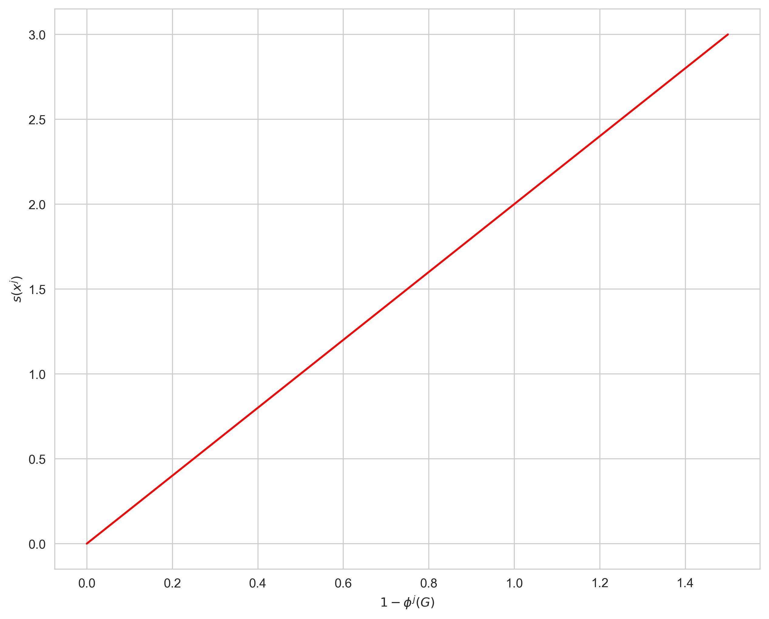
(a) $f_{s}^{1}(\cdot)$

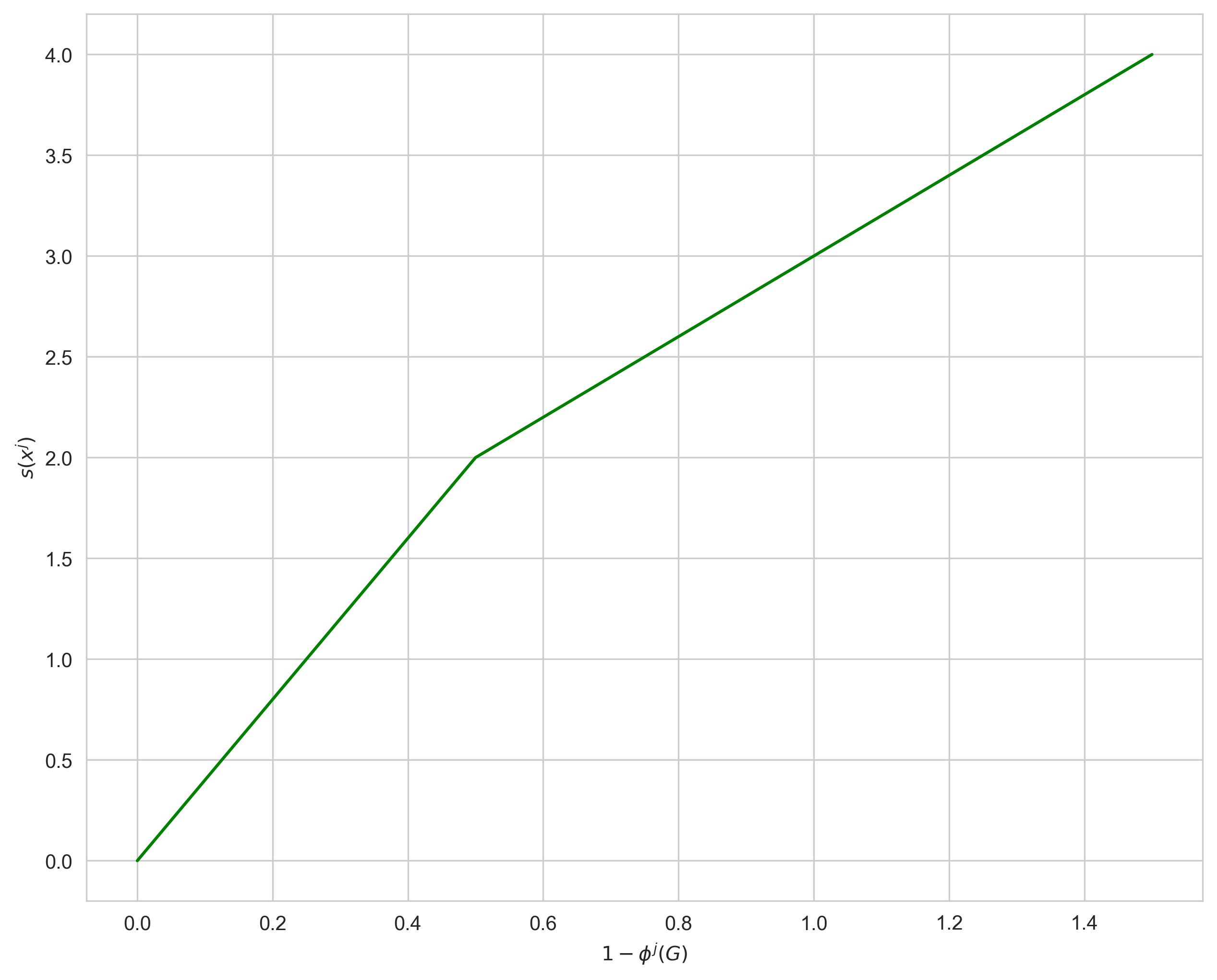
(b) $f_{s}^{2}(\cdot)$

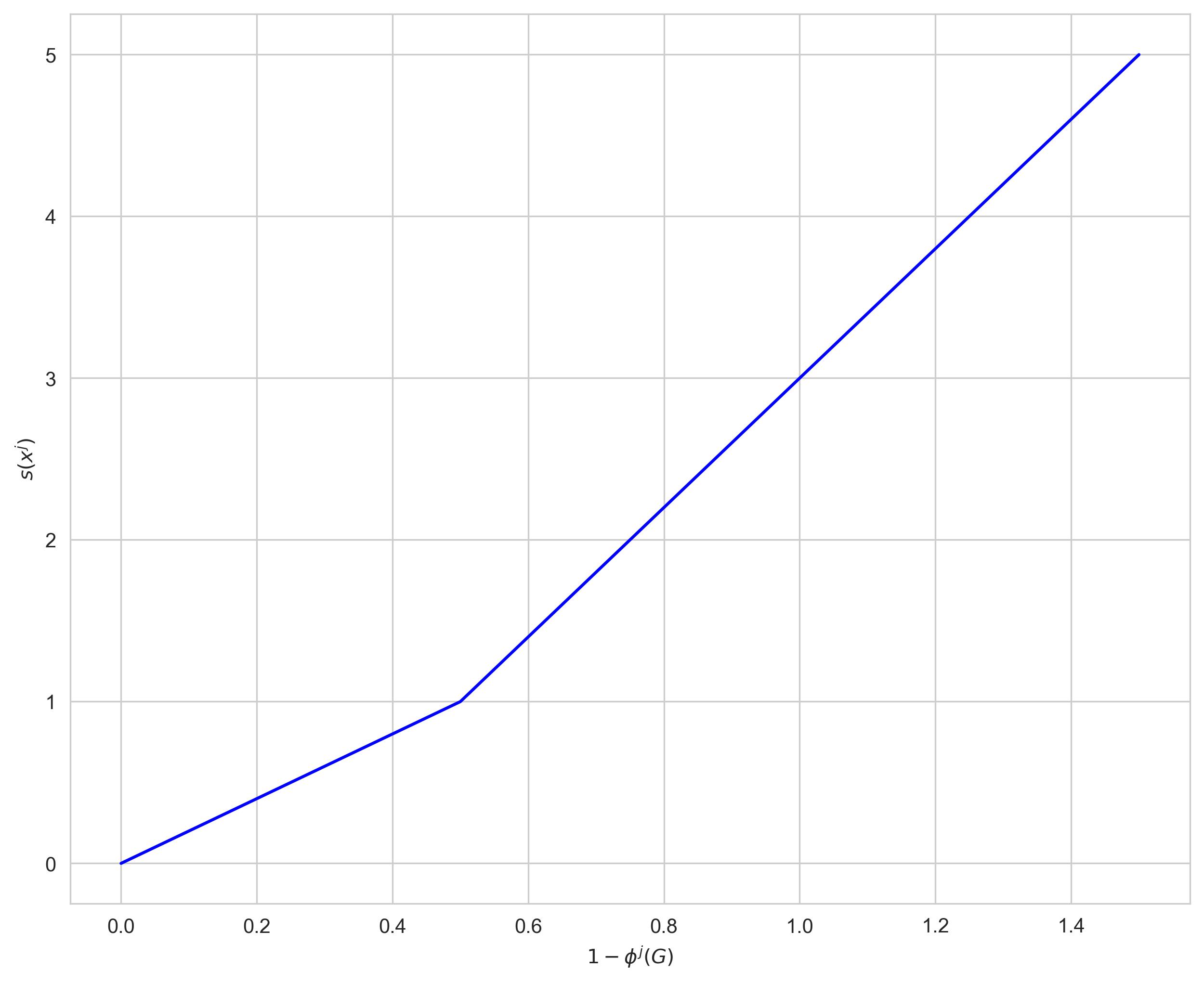
(c) $f_{s}^{3}(\cdot)$

Figure 7: Different function $f_{s}(\cdot)$ in sample-level method.

Method	Accuracy
	Kinetics Sounds	UCF-101
Concatenation	62.30	81.15
Decision fusion	62.65	79.81
$f_{s}^{1}(\cdot)$	66.92	83.52
$f_{s}^{2}(\cdot)$	68.58	83.12
$f_{s}^{2}(\cdot)$	67.12	83.68

(a) Sample-level method.

Method	Accuracy
	Kinetics Sounds	UCF-101
Concatenation	62.30	81.15
Decision fusion	62.65	79.81
$f_{m}(d)=d$	66.65	83.46
$f_{m}(d)=\text{tanh}(d)$	66.50	83.86
$f_{m}(d)=\text{power}(1.5,d)$	65.69	83.25

(b) Modality-level method.

Table 7: Comparison with different function $f(\cdot)$.

Method	UCF-101
	Acc	Num of re-sampled samples
Concatenation	81.15	-
Decision fusion	79.81	-
Low re-sample rate	83.41	$0.96\times$
High resample rate	82.24	$2.68\times$
Ours	83.52	$1.00\times$

Table 8: Comparison with fixed re-sample rate methods on the UCF-101 dataset.

Appendix I Experiments of fixed re-sample rate

In our methods, the specific re-sample rate is dynamically determined by the exact contribution value during training. Concretely, the low-contributing modality in sample $x$ is re-trained with a re-sample rate inversely proportional to its contribution. To validate the effectiveness of our method, we perform experiments of fixed re-sample rate on the UCF-101 dataset and the results are shown in Table 8. Two types of fixed re-sample rate methods are compared: low re-sample rate one and high re-sample rate one. Both the performance of low re-sample rate method and high re-sample rate method are inferior to our method. In addition, compared to our method, the number of re-sampled samples of low re-sample rate method is close, since the dataset has a long-tail phenomenon that the contribution of low-contributing modality in the majority of samples is not severely low. But the number of re-sampled samples of high re-sample rate method is obviously greater but with worse performance. The reason could be that the high re-sample rate leads to more server over-fitting. These experiments indicate the effectiveness of our dynamic re-sample rate.

References

- Ando and Huang (2017) Ando, S.; and Huang, C. Y. 2017. Deep over-sampling framework for classifying imbalanced data. In Machine Learning and Knowledge Discovery in Databases: European Conference, ECML PKDD 2017, Skopje, Macedonia, September 18–22, 2017, Proceedings, Part I 10, 770–785. Springer.
- Arandjelovic and Zisserman (2017) Arandjelovic, R.; and Zisserman, A. 2017. Look, listen and learn. In Proceedings of the IEEE International Conference on Computer Vision, 609–617.
- Baltrušaitis, Ahuja, and Morency (2018) Baltrušaitis, T.; Ahuja, C.; and Morency, L.-P. 2018. Multimodal machine learning: A survey and taxonomy. IEEE transactions on pattern analysis and machine intelligence, 41(2): 423–443.
- Blundell et al. (2015) Blundell, C.; Cornebise, J.; Kavukcuoglu, K.; and Wierstra, D. 2015. Weight uncertainty in neural network. In International conference on machine learning, 1613–1622. PMLR.
- Chen et al. (2020) Chen, H.; Xie, W.; Vedaldi, A.; and Zisserman, A. 2020. Vggsound: A large-scale audio-visual dataset. In ICASSP 2020-2020 IEEE International Conference on Acoustics, Speech and Signal Processing (ICASSP), 721–725. IEEE.
- Devlin et al. (2018) Devlin, J.; Chang, M.-W.; Lee, K.; and Toutanova, K. 2018. Bert: Pre-training of deep bidirectional transformers for language understanding. arXiv preprint arXiv:1810.04805.
- Freund and Schapire (1996) Freund, Y.; and Schapire, R. E. 1996. Game theory, on-line prediction and boosting. In Proceedings of the ninth annual conference on Computational learning theory, 325–332.
- Gemp et al. (2020) Gemp, I.; McWilliams, B.; Vernade, C.; and Graepel, T. 2020. EigenGame: PCA as a Nash Equilibrium. In International Conference on Learning Representations.
- Ghorbani and Zou (2020) Ghorbani, A.; and Zou, J. Y. 2020. Neuron shapley: Discovering the responsible neurons. Advances in Neural Information Processing Systems, 33: 5922–5932.
- He et al. (2016) He, K.; Zhang, X.; Ren, S.; and Sun, J. 2016. Deep residual learning for image recognition. In Proceedings of the IEEE conference on computer vision and pattern recognition, 770–778.
- Hu, Li, and Zhou (2022) Hu, P.; Li, X.; and Zhou, Y. 2022. SHAPE: An Unified Approach to Evaluate the Contribution and Cooperation of Individual Modalities. arXiv preprint arXiv:2205.00302.
- Huang et al. (2022) Huang, Y.; Lin, J.; Zhou, C.; Yang, H.; and Huang, L. 2022. Modality Competition: What Makes Joint Training of Multi-modal Network Fail in Deep Learning?(Provably). arXiv preprint arXiv:2203.12221.
- Joze et al. (2020) Joze, H. R. V.; Shaban, A.; Iuzzolino, M. L.; and Koishida, K. 2020. MMTM: Multimodal transfer module for CNN fusion. In Proceedings of the IEEE/CVF Conference on Computer Vision and Pattern Recognition, 13289–13299.
- Kay et al. (2017) Kay, W.; Carreira, J.; Simonyan, K.; Zhang, B.; Hillier, C.; Vijayanarasimhan, S.; Viola, F.; Green, T.; Back, T.; Natsev, P.; et al. 2017. The kinetics human action video dataset. arXiv preprint arXiv:1705.06950.
- Kiela et al. (2018) Kiela, D.; Grave, E.; Joulin, A.; and Mikolov, T. 2018. Efficient large-scale multi-modal classification. In Proceedings of the AAAI conference on artificial intelligence, volume 32.
- Nagrani et al. (2021) Nagrani, A.; Yang, S.; Arnab, A.; Jansen, A.; Schmid, C.; and Sun, C. 2021. Attention bottlenecks for multimodal fusion. Advances in Neural Information Processing Systems, 34: 14200–14213.
- Nefian et al. (2002) Nefian, A. V.; Liang, L.; Pi, X.; Liu, X.; and Murphy, K. 2002. Dynamic Bayesian networks for audio-visual speech recognition. EURASIP Journal on Advances in Signal Processing, 2002(11): 1–15.
- Neumann, Zisserman, and Vedaldi (2018) Neumann, L.; Zisserman, A.; and Vedaldi, A. 2018. Relaxed softmax: Efficient confidence auto-calibration for safe pedestrian detection.
- Ngiam et al. (2011) Ngiam, J.; Khosla, A.; Kim, M.; Nam, J.; Lee, H.; and Ng, A. Y. 2011. Multimodal deep learning. In ICML.
- Owens and Efros (2018) Owens, A.; and Efros, A. A. 2018. Audio-visual scene analysis with self-supervised multisensory features. In Proceedings of the European Conference on Computer Vision (ECCV), 631–648.
- Peng et al. (2022) Peng, X.; Wei, Y.; Deng, A.; Wang, D.; and Hu, D. 2022. Balanced Multimodal Learning via On-the-fly Gradient Modulation. In Proceedings of the IEEE/CVF Conference on Computer Vision and Pattern Recognition, 8238–8247.
- Perez et al. (2018) Perez, E.; Strub, F.; De Vries, H.; Dumoulin, V.; and Courville, A. 2018. Film: Visual reasoning with a general conditioning layer. In Proceedings of the AAAI conference on artificial intelligence, volume 32.
- Poria, Cambria, and Gelbukh (2015) Poria, S.; Cambria, E.; and Gelbukh, A. 2015. Deep convolutional neural network textual features and multiple kernel learning for utterance-level multimodal sentiment analysis. In Proceedings of the 2015 conference on empirical methods in natural language processing, 2539–2544.
- Poria et al. (2018) Poria, S.; Hazarika, D.; Majumder, N.; Naik, G.; Cambria, E.; and Mihalcea, R. 2018. Meld: A multimodal multi-party dataset for emotion recognition in conversations. arXiv preprint arXiv:1810.02508.
- Shapley (1953) Shapley, L. S. 1953. 17. A Value for n-Person Games.
- Sikka et al. (2013) Sikka, K.; Dykstra, K.; Sathyanarayana, S.; Littlewort, G.; and Bartlett, M. 2013. Multiple kernel learning for emotion recognition in the wild. In Proceedings of the 15th ACM on International conference on multimodal interaction, 517–524.
- Simonyan and Zisserman (2014) Simonyan, K.; and Zisserman, A. 2014. Two-stream convolutional networks for action recognition in videos. Advances in neural information processing systems, 27.
- Soomro, Zamir, and Shah (2012) Soomro, K.; Zamir, A. R.; and Shah, M. 2012. UCF101: A dataset of 101 human actions classes from videos in the wild. arXiv preprint arXiv:1212.0402.
- Tian et al. (2018) Tian, Y.; Shi, J.; Li, B.; Duan, Z.; and Xu, C. 2018. Audio-visual event localization in unconstrained videos. In Proceedings of the European Conference on Computer Vision (ECCV), 247–263.
- Van der Maaten and Hinton (2008) Van der Maaten, L.; and Hinton, G. 2008. Visualizing data using t-SNE. Journal of machine learning research, 9(11).
- Vielzeuf et al. (2018) Vielzeuf, V.; Lechervy, A.; Pateux, S.; and Jurie, F. 2018. Centralnet: a multilayer approach for multimodal fusion. In Proceedings of the European Conference on Computer Vision (ECCV) Workshops, 0–0.
- Wang et al. (2017) Wang, K.; Gou, C.; Duan, Y.; Lin, Y.; Zheng, X.; and Wang, F.-Y. 2017. Generative adversarial networks: introduction and outlook. IEEE/CAA Journal of Automatica Sinica, 4(4): 588–598.
- Wang, Tran, and Feiszli (2020) Wang, W.; Tran, D.; and Feiszli, M. 2020. What makes training multi-modal classification networks hard? In Proceedings of the IEEE/CVF Conference on Computer Vision and Pattern Recognition, 12695–12705.
- Wang (2021) Wang, Y. 2021. Survey on deep multi-modal data analytics: Collaboration, rivalry, and fusion. ACM Transactions on Multimedia Computing, Communications, and Applications (TOMM), 17(1s): 1–25.
- Wu et al. (2022) Wu, N.; Jastrzebski, S.; Cho, K.; and Geras, K. J. 2022. Characterizing and overcoming the greedy nature of learning in multi-modal deep neural networks. In International Conference on Machine Learning, 24043–24055. PMLR.
- Xu, Zhu, and Clifton (2023) Xu, P.; Zhu, X.; and Clifton, D. A. 2023. Multimodal learning with transformers: A survey. IEEE Transactions on Pattern Analysis and Machine Intelligence.
- Zhao et al. (2018) Zhao, H.; Gan, C.; Rouditchenko, A.; Vondrick, C.; McDermott, J.; and Torralba, A. 2018. The sound of pixels. In Proceedings of the European conference on computer vision (ECCV), 570–586.
- Zhu et al. (2021) Zhu, H.; Luo, M.-D.; Wang, R.; Zheng, A.-H.; and He, R. 2021. Deep audio-visual learning: A survey. International Journal of Automation and Computing, 18(3): 351–376.