Reconstruction Formulae for 3D Field-Free Line Magnetic Particle Imaging

Abstract

Magnetic Particle Imaging (MPI) is a promising noninvasive in vivo imaging modality that makes it possible to map the spatial distribution of superparamagnetic nanoparticles by exposing them to dynamic magnetic fields. In the Field-Free Line (FFL) scanner topology, the spatial encoding of the particle distribution is performed by applying magnetic fields vanishing on straight lines. The voltage induced in the receiving coils by the particles when exposed to the magnetic fields constitute the signal from which the particle distribution is to be reconstructed. To avoid lengthy calibration, model-based reconstruction formulae have been developed for the 2D FFL scanning topology. In this work we develop reconstruction formulae for 3D FFL. Moreover, we provide a model-based reconstruction algorithm for 3D FFL and we validate it with a numerical experiment.

1 Introduction

Magnetic Particle Imaging (MPI) is a promising medical imaging modality that allows to reconstruct the distribution of superparamagnetic nanoparticles by exploiting their non-linear magnetization response to dynamic magnetic fields. The principles behind MPI have been introduced by Gleich and Weizenecker in their seminal paper published in Nature in 2005 [17] and led them and their team to win the European Inventor Award in 2016. In 2009, Weizenecker et al. [65] successfully managed to produce a video (3D+time) of a distribution of a clinically approved MRI contrast agent flowing through the beating heart of a mouse, thereby taking an important step towards medical applications of MPI and in particular towards its applicability to 3D real-time in vivo imaging. Since then, interest in the technology has been on the rise, as has the number of medical applications. These include multimodal imaging [1], cancer detection (of as few as 250 cancer cells [49]) and cancer imaging [1, 12, 55, 68], (stem) cell tracing [11, 19, 27, 38, 57], inflammation tracing and lung perfusion imaging [69], drug delivery and monitoring [70], cardiovascular [2, 58, 61] and blood flow [14] imaging, tracking of medical instruments [22], brain injury detection [43] as well as future MPI-assisted stroke detection and brain monitoring made possible by a recently developed human-sized MPI scanner [21]. The high degree of applicability of MPI is due to its benefits, including quatifyability and high sensitivity, and due to its advantages over other imaging modality such as CT [8], MRI [48], PET [56] and SPECT [36], for example, its ability to provide higher spatial resolution in a shorter acquisition time and the absence of radiation or radioactive tracers, making it a safer imaging option [31]. Deeper comparison between existing imaging modalities and MPI as well as further examples of state-of-the-art applications can be found in [5, 67].

In brief, the principle and the procedure behind MPI are as follows: (i) the specimen to be scanned is injected with a tracer containing the magnetic nanoparticles (MNs); (ii) a dynamic magnetic field with a low-field volume (LFV) is applied and the LFV is spatially moved; (iii) because the response of the MNs is nonlinear precisely where the field is close to zero, the LFV acts as a sensitive region whose motion causes the particles to induce a voltage in the receiver coils, a voltage that constitutes the signal that encodes the information about the particles’ position and concentration. The imaging task of MPI is the reconstruction of the spatial distribution of the particles in the tracer from the signal (voltage) acquired during a scan.

Concerning the LFVs employed, the first possibility explored [17] is the case when the dynamic magnetic field applied is the superposition of a static field with a point where the field vanishes - the Field-Free Point (FFP) - and a dynamic field that steers the FFP along some trajectory in the scanning region - or Field of View (FoV). There are currently two main approaches to reconstructing distributions with the FFP topology: a measurement-based approach and a model-based approach. In the measurement-based approach a 3D grid (tessellation with cubic cells) of the volume to be scanned inside the scanner’s bore is considered; a probe with a reference concentration of tracer is iteratively positioned and scanned at each voxel, i.e., at each cubic cell constituting the grid. This way the response of the scanning system to discrete Dirac delta impulses (the point spread function [4]) at each voxel position is collected in a system matrix, which should ideally describe the linear relationship between discrete (according to the chosen grid) distributions and the acquired signal. The reconstruction idea is, given the MPI signal collected, to invert the system matrix (with regularization techniques due to the presence of noise and the ill-conditioning of the matrix) to obtain a discretized reconstruction of the target distribution [34, 52]. The acquisition of the system matrix (calibration) is time-consuming and while effort has been put into the research of ways to speed up this procedure [30, 37, 46], other solutions have been investigated that avoid the lengthy calibration and are model based. Indeed, model-based approaches are an active area of research in MPI and try to provide reconstruction formulae for various MPI setups. In the particular case of the FFP topology, at first reconstruction formulae were available only for 1D scans [45] but were followed soon after by the so-called $X$-space formulation for the 1D [18] scans and later for the multidimensional case [19]. Using this formulation the authors derived reconstruction formulae for the 2D and 3D FFP case [40] and formulate a two-stage algorithm that has been recently further developed [15] and made flexible enough to deal with multi-patching scans [16].

Concerning other scanning topologies, in 2008 Weizenecker, Gleich and Borgert proposed a Field-Free Line (FFL) scan modality, i.e., the employment of magnetic fields vanishing on a line, with the promise of a more effective encoding scheme, an increase in sensitivity of acquisition, a greater signal to noise ratio (SNR) [64] and potentially a lower level of ill-posedness for the inverse problem underlying the reconstruction task in MPI with FFL as opposed to the FFP topology [29]. At first, there were doubts about the feasibility of a FFL scanner, but Knopp et al. [13, 32, 35] showed that it is possible to produce a system with power dissipation comparable to that of a FFP scanner. Soon after, the first 2D images with a FFL scanner were made possible [20]. In 2014 the first continuously rotated FFL scanner has been presented by Weber et al. [3]. Since then, effort has been put into the study of possible human-sized FFL scanners [6] and into the design of animal-sized scanners [10, 41]. As for the FFP topology, reconstruction with FFL data can be done by either acquiring a system matrix or using model-based approaches [24]. The measurement-based approach works in the same way as with the FFP topology: a reference concentration that plays the role of a Dirac delta distribution is placed and scanned in each voxel position and the data thus acquired form the system matrix; regularized inversion of the system matrix produces a reconstruction of the target distribution (examples of measurement-based reconstructions for 2D FFL can be found in [24, 28, 60]). Much more attention have received model-based approaches for FFL, thanks to the link with the Radon transform and consequent availability of a Fourier slice theorem for model-based 2D reconstructions [33]. This is beneficial because the theory of the Radon transform [23, 44, 39] and its inversion in 2D is well studied in the context of CT [42] and offers a plethora of well-established classical techniques [66] as well as more recent Machine Learning-based methods [54] that become available for model-based reconstructions in MPI. Thanks to recent developments of the scanner, it is possible to both rotate the FFL and translate it in 3D [59] and this flexibility has been employed for the first simulation of FFL 3D scans. Indeed, by scanning in a slice-wise fashion [50] the Radon-based reconstruction formulae for 2D FFL applied to each slice can be used to reconstruct 3D distributions. Scanning trajectories for 3D FFL have also been investigated and utilized with the system-matrix-based approach [51] but to the best of our knowledge, no fully 3D FFL reconstruction formulae exists to date. Before describing the contributions of this paper and its outline, we would like to briefly discuss a further reason why model-based approaches for FFL scans in 3D setups are an interesting and important direction of research. In all generality, the Radon transform is a transform that considers integrals on hyperplanes in spaces of any dimension [39] and reconstruction formulae analogous to the 2D case exist for the 3D case if we consider integrals on planes [42]. In MPI this translates into considering magnetic fields with a Field-Free Plane, instead of a FFL. However, a Field-Free Plane is not possible due to Maxwell’s equations (a proof of this fact can be found in  Section 2). As a consequence, the maximum dimensionality of possible FFRs (Field-Free Regions) in MPI is 1, which corresponds to the FFL topology and this fact underlines the importance of model-based approaches for 3D FFL scans.

Contributions

The purpose of this paper is to provide model-based reconstruction approaches for a proposed 3D FFL scanning scheme. In particular, we make the following major contributions:

• we provide model-based reconstruction formulae for 3D FFL MPI;

• we provide a reconstruction algorithm for 3D FFL and illustrate its applicability with a numerical example.

Outline of the Paper

We begin our work by recalling the physical modeling of MPI in Section 2, where we also describe the possible scanner topologies and prove that Field-Free Plane topologies are not possible as a consequence of Maxwell’s equations. In Section 3 we describe the proposed 3D FFL scanning setup and we prove the main result of this paper from which we derive the reconstruction formulae. In Section 4 we describe the three steps of the proposed reconstruction algorithm and in Section 5 we show a numerical experiment that illustrates the reconstruction algorithm. We conclude with a discussion of the results and future research directions in Section 6.

2 Particle Magnetization, Induced Signal and Scanner Topologies

We now describe the physical model that puts the magnetization response of the particles when exposed to dynamic magnetic fields in relation to the voltage induced in the receiving coils of the scanner.

Particle Magnetization

Let $\rho\colon\mathbb{R}^{3}\to\mathbb{R}^{+}$ be a distribution of superparamagnetic particles exposed to a dynamic magnetic field $\bm{H}\colon\mathbb{R}^{3}\times\mathbb{R}\to\mathbb{R}^{3}$ with $(\bm{x},t)\mapsto\bm{H}(\bm{x},t)$. Assuming instantaneous remagnetization of the particles, the magnetization is modeled according to the Langevin theory of paramagnetism [9, 26] as follows:

$$\bm{M}(\bm{x},t)=m\rho(\bm{x})\mathcal{L}\biggl{(}\frac{\lVert\bm{H}(\bm{x},t)\rVert}{H_{\mathrm{sat}}}\biggr{)}\frac{\bm{H}(\bm{x},t)}{\lVert\bm{H}(\bm{x},t)\rVert},\quad\text{with }H_{\mathrm{sat}}=\frac{k_{B}T}{\mu_{0}M_{\mathrm{sat}}\frac{\pi}{6}d^{3}},$$ (1)

where $m$ is the magnetic moment of a single particle, $k_{B}$ is the Boltzmann constant, $T$ the temperature of the particles, $\mu_{0}$ is the magnetic permeability, $M_{\mathrm{sat}}$ the saturation magnetization, $d$ is the particles’ diameter and $\mathcal{L}$ is the Langevin function $\mathcal{L}(x)=\coth(x)-\frac{1}{x}$.

Signal Encoding

Let now $\bm{u}(t)$ be the voltage received by the three receive coils and $P\colon\mathbb{R}^{3}\to\mathbb{R}^{3\times 3}$ be their sensitivity pattern. According to Faraday’s law of induction, the voltage induced in the coils is the negative rate of change of the magnetic flux $\bm{\Phi}(t)$:

$$\bm{u}(t)=-\frac{d}{dt}\bm{\Phi}(t),\quad\text{where }\bm{\Phi}(t)=\mu_{0}\int_{\mathbb{R}^{3}}P(\bm{x})\bigl{(}\bm{H}(\bm{x},t)+\bm{M}(\bm{x},t)\bigr{)}\,d\bm{x}.$$ (2)

Because only the magnetization term $\bm{M}$ in Equation 2 is related to distribution $\rho$, see Equation 1, after subtracting from $\bm{u}(t)$ the signal of an empty scan, i.e., a scan with $\rho(\bm{x})=0$, we obtain the signal:

$$\bm{s}(t)=-\mu_{0}\frac{d}{dt}\int_{\mathbb{R}^{3}}P(\bm{x})\bm{M}(\bm{x},t)\,d\bm{x}.$$ (3)

Possible Scanner Topologies

From Equations 3 and 1 it is clear that the signal $\bm{s}(t)$ induced in the receiving coils during a scan depends on the derivative of the Langevin function, which is a bell-shaped function with maximum in $0$ and asymptotically zero away from $0$. This means that the regions that produce the highest amount of signal are those close to the set of points where the magnetic field vanishes, the so-called Field-Free Region (FFR). The shape of the FFR defines the topology (or geometry) of the MPI scanner employed. The MPI principle has been introduced by Weizenecker and Gleich [17] considering magnetic fields vanishing in a single point. This is known as the Field-Free Point (FFP) topology and model-based reconstruction formulae in 2D and 3D have been proposed by the authors [40].

It is also possible to consider the Field-Free Line (FFL) topology, i.e., scanners employing magnetic fields vanishing along a line. The FFL topology has been introduced in [64] and has been tightly connected to the theory of the Radon transform in 2D and in particular, a Fourier slice theorem has been proved and provides reconstruction formulas for 2D scans [33]. The Radon transform [44, 42] is an integral transform that represents functions $f\colon\mathbb{R}^{n}\to\mathbb{R}$ (in a suitable space) through the integrals of $f$ on affine hyperplanes $\mathbf{L}$ of $\mathbb{R}^{n}$,i.e., on affine subspaces of dimension $n-1$. One then would expect that a natural generalization of the 2D Field Free Line topology in 3D would be a Field Free Plane topology. The authors in [64] have mentioned that it is not possible to have magnetic fields vanishing on a plane, as Maxwell’s equations [25] put physical limitations to the magnetic fields that can occur. We have not however found a proof of this statement in the literature and we provide one to formally motivate our choice to focus on the FFL topology and set aside the study of the Radon transform on planes in the context of MPI. The result is based on the following property of sinusoidal and irrotational fields:

Theorem 1.

Let $\Omega\subset\mathbb{R}^{3}$ be a non empty and connected open set, $\bm{H}\colon\Omega\to\mathbb{R}^{3}$ be a continuously differentiable vector field satisfying the differential equations:

$$\nabla\cdot\bm{H} =0,$$ (4)

$$\nabla\times\bm{H} =0.$$ (5)

Then, level sets of $\bm{H}$ cannot be ($2$-dimensional) regular surfaces in $\Omega$.

Proof.

Suppose for the sake of contradiction that $\bm{H}$ is constant on some $2$-dimensional regular surface in $\Omega$, i.e., there exists a $2$-dimensional regular surface $\mathcal{S}\subset\Omega$ and a constant $\bm{c}\in\mathbb{R}^{3}$ such that in each point $\bm{x}_{0}\in\mathcal{S}$ it holds $\bm{H}(\bm{x}_{0})=\bm{c}$ and the tangent space $T_{\bm{x}_{0}}\mathcal{S}$ is 2-dimensional. Given a point $\bm{x}_{0}\in\mathcal{S}$, let $\varphi(\tau,\sigma)$ be a surface parametrization of $\mathcal{S}$ with:

$$\begin{cases}\varphi(0,0)=\bm{x}_{0}\\ \partial_{\tau}\varphi(0,0)=\bm{v}\\ \partial_{\sigma}\varphi(0,0)=\bm{u}\end{cases},$$ (6)

for some linearly independent vectors $\bm{u}$ and $\bm{v}$. Let $\bm{J_{H}}$ be the Jacobian matrix of $\bm{H}$, $(\bm{J_{H}})_{i,j}=\frac{\partial H_{i}}{\partial x_{j}}$. Because $\bm{H}\left(\varphi(\tau,\sigma)\right)=\bm{c}$, we get that $\bm{J_{H}}(\bm{x}_{0})\bm{v}=0$ and $\bm{J_{H}}(\bm{x}_{0})\bm{u}=0$, which in turn means that $\bm{J_{H}}(\bm{x}_{0})$ has eigenvalue $0$ with geometric multiplicity of $2$. In turn, also the algebraic multiplicity must be at least $2$, meaning that if $\lambda_{1}$, $\lambda_{2}$, $\lambda_{3}$ are the eigenvalues of $\bm{J_{H}}(\bm{x}_{0})$, then two of them are zero. Without loss of generality, we can consider $\lambda_{1}=\lambda_{2}=0$. Now, we combine the hypothesis in Equation 4 with the fact that the divergence of the field is the trace of the Jacobian, i.e.,

$$0=\nabla\cdot\bm{H}(\bm{x}_{0})=\operatorname{trace}\left(\bm{J_{H}}(\bm{x}_{0})\right)=\lambda_{1}+\lambda_{2}+\lambda_{3}=0+0+\lambda_{3},$$ (7)

which forces $\lambda_{3}=0$ as well and shows that $0$ is an eigenvalue with algebraic multiplicity of $3$.

On the other hand, Equation 5 implies that $\bm{J_{H}}(\bm{x}_{0})$ is symmetric and therefore diagonalizable. Diagonalizability of a matrix is equivalent to the fact that the algebraic and geometric multiplicities of each eigenvalue are equal, which proves that the geometric multiplicity of $\bm{J_{H}}(\bm{x}_{0})$ is also of $3$ and consequently, that $\bm{J_{H}}(\bm{x}_{0})=0$. Finally, on a regular surface the tangent space is isomorphic to the kernel of the Jacobian, i.e., $\bm{J_{H}}(\bm{x}_{0})\cong T_{\bm{x}_{0}}\mathcal{S}$, but this leads to a contradiction: the tangent space on a $2$-dimensional regular surface is always $2$-dimensional, while we have proved that the Jacobian has always a $3$-dimensional kernel on $\mathcal{S}$. ∎

Corollary 1.

Magnetic Particle Imaging with a Field-Free Plane topology is not possible.

Proof.

Magnetic fields must obey Maxwell’s equations and in the particular case of fields without magnetic field sources and without magnetization - as in the fields produced inside an MPI scanner - fulfill both magneto-static and quasi-static approximations [6]. This translates mathematically into the fact that the fields satisfy Equations 4 and 5. A Field-Free Plane is a $2$-dimensional regular surface defined as the level set $\{\bm{x}\in\Omega\colon\bm{H}(\bm{x})=0\}$, which is impossible by 1. ∎

In view of this result and of the fact that it is possible to move and rotate the FFL in any position in space [35, 51], we will consider the FFL topology and propose model-based reconstruction formulae for 3D FFL MPI.

3 Field-Free Line Magnetic Particle Imaging in 3D

In this section we introduce our proposed scanning setup for 3D FFL scans, the FFL MPI Core Operator and the results that allow us to formulate the sought reconstruction formulae. We start by describing our proposed 3D FFL scanning modality which is based on the model employed to generate FFLs on a plane [35, 33]. Because we build our proposed scanning modality on the modeling of magnetic fields employed in the 2D FFL, we start by recalling its mathematical formulation.

Consider the frame of reference $(x,y,z)$ of the scanner. We will denote from now on with $\bm{e}_{x}$ the unitary vector in the direction of the $x$-axis and $\bm{e}_{y}$,$\bm{e}_{z}$ analogously. The static magnetic field with a FFL along the $x$-axis and gradient strength $G\in\mathbb{R}$ has the following expression [33, 35]:

$$\bm{H}_{S}^{0}(\bm{x})=G\begin{pmatrix}0&0&0\\ 0&-1&0\\ 0&0&1\end{pmatrix}\bm{x}.$$

Consider a rotation angle $\theta\in[0,2\pi)$, the magnetic field $\bm{H}_{S}^{\theta}$ obtained by rotating counterclockwise $\bm{H}_{S}^{0}$ in the $xy$-plane by $\theta$ can be written as:

$$\bm{H}_{S}^{\theta}(\bm{x})=GR_{\theta}\begin{pmatrix}0&0&0\\ 0&-1&0\\ 0&0&1\end{pmatrix}R_{\theta}^{T}\bm{x},$$ (8)

where $R_{\theta}$ is the rotation matrix

$$R_{\theta}=\begin{pmatrix}\cos\theta&-\sin\theta&0\\ \sin\theta&\cos\theta&0\\ 0&0&1\end{pmatrix}.$$ (9)

Let now $(\bm{e}_{\theta},\bm{e}_{\theta}^{\perp},\bm{e}_{z})$ be the orthonormal rotated basis consisting of the columns of $R_{\theta}$, i.e., $\bm{e}_{\theta}=(\cos\theta,\sin\theta,0)^{T}$, $\bm{e}_{\theta}^{\perp}=(-\sin\theta,\cos\theta,0)^{T}$ and $\bm{e}_{z}$. We can write the components of the static field $\bm{H}_{S}^{\theta}$ with respect to the rotated basis by simply performing the matrix multiplications in Equation 8:

$$\begin{split}\bm{H}_{S}^{\theta}(\bm{x})&=G(x\sin\theta-y\cos\theta)\bm{e}_{\theta}^{\perp}+Gz\bm{e}_{z}\\ &=-G\langle\bm{x}\,,\bm{e}_{\theta}^{\perp}\rangle\bm{e}_{\theta}^{\perp}+G\langle\bm{x}\,,\bm{e}_{z}\rangle\bm{e}_{z},\end{split}$$ (10)

where $\langle\cdot\,,\cdot\rangle$ is the standard scalar product. In the 2D scenario, to move the FFL in the $xy$-plane while keeping it parallel to the $\bm{e}_{\theta}$ direction, an oscillating dynamic field $\bm{H}_{D}^{\theta}$ along the orthogonal direction $\bm{e}_{\theta}^{\perp}$ is added:

$$\bm{H}_{D}^{\theta}(t)=A\Lambda(t)\bm{e}_{\theta}^{\perp},$$ (11)

with $\Lambda(t)$ usually chosen to be sinusoidal [33] of amplitude $A$, e.g., $\Lambda(t)=\cos(2\pi f_{0}t)$ for some excitation frequency $f_{0}$. Hence, the magnetic field applied for a scan given an angle $\theta$ is the superposition of the static and dynamic fields:

$$\bm{H}^{\theta}(\bm{x},t)=\bm{H}_{S}^{\theta}(\bm{x})+\bm{H}_{D}^{\theta}(t).$$ (12)

3.1 Proposed Scanning Setup

We now describe a possible purely 3D FFL scanning modality. Our idea is to consider the 2D FFL setup in the $xy$-plane described in Equation 12 with dynamic field applied as in Equation 11 and allow movement of the FFL also along the $z$-axis (this is possible in view of the recent results in [51]). Therefore, given an angle $\theta$ and a static magnetic field $\bm{H}_{S}^{\theta}(\bm{x})$ as in Equation 8, we consider the following dynamic field:

$$\bm{H}_{D}^{\theta}(t)=A_{1}\Lambda_{1}(t)\bm{e}_{\theta}^{\perp}-A_{2}\Lambda_{2}(t)\bm{e}_{z},$$ (13)

with sinusoidal functions $\Lambda_{1}$,$\Lambda_{2}$ and amplitudes $A_{1}$,$A_{2}$. The magnetic field applied to the particle distribution in this 3D FFL scan is therefore:

$$\begin{split}\bm{H}^{\theta}(\bm{x},t)&=\bm{H}_{S}^{\theta}(\bm{x})+\bm{H}_{D}^{\theta}(t)\\ &=\left(A_{1}\Lambda_{1}(t)-G\langle\bm{x},\bm{e}_{\theta}^{\perp}\rangle\right)\bm{e}_{\theta}^{\perp}+\left(-A_{2}\Lambda_{2}(t)+Gz\right)\bm{e}_{z}.\end{split}$$ (14)

Using Equations 2 and 3 and assuming that the receive coil sensitivity pattern is constant,i.e., $P(\bm{x})=P\in\mathbb{R}^{3\times 3}$, the signal obtained during a scan applying the magnetic field $\bm{H}^{\theta}(\bm{x},t)$ is given by:

$$\bm{s}^{\theta}(t)=-\mu_{0}mP\frac{d}{dt}\int_{\mathbb{R}^{3}}\rho(\bm{x})\mathcal{L}\biggl{(}\frac{\lVert\bm{H}^{\theta}(\bm{x},t)\rVert}{H_{\mathrm{sat}}}\biggr{)}\frac{\bm{H}^{\theta}(\bm{x},t)}{\lVert\bm{H}^{\theta}(\bm{x},t)\rVert}\,d\bm{x}.$$ (15)

3.2 Decomposition of the Signal and the MPI Core Operator in the FFL setting

In this section we state and prove the main results of this work (3). In particular, we show that for the 3D FFL scan proposed with the magnetic fields as in Equation 14 the signal obtained is related to the distribution $\rho$ via the MPI Core Operator and the X-Ray projection operator. Before stating the theorem we recall some important mathematical tools needed for its formulation.

The first fundamental tool we recall is the (Field-Free Point) MPI Core Operator [40], of which we give here a generalized definition on affine subspaces of $\mathbb{R}^{3}$:

Definition 2.

Given a distribution $\rho\in L_{2}\left(\Omega\,;\mathbb{R}^{+}\right)$ and an affine subspace $\mathbf{L}$ with $\dim\mathbf{L}=n\in\{2,3\}$ in $\mathbb{R}^{3}$ we define the MPI Core Operator as the operator $A_{\mathbf{L},h}[\,\cdot\,]\,\colon L_{2}\left(\Omega\,;\mathbb{R}^{+}\right)\to L_{2}\left(\Omega\cap\mathbf{L}\,;\mathbb{R}^{n\times n}\right)$ given by $\rho\mapsto A_{\mathbf{L},h}[\rho]\colon\Omega\cap\mathbf{L}\to\mathbb{R}^{n\times n}$ where:

$$\bm{r}\mapsto A_{\mathbf{L},h}[\rho](\bm{r})\coloneq\int_{\mathbf{L}\cap\Omega}\rho(\bm{x})\nabla_{\bm{r}}\left(\mathcal{L}\biggl{(}\frac{\lVert\bm{r}-\bm{x}\rVert}{h}\biggr{)}\frac{\bm{r}-\bm{x}}{\lVert\bm{r}-\bm{x}\rVert}\right)\,d\bm{S}(\bm{x}).$$ (16)

In case that $n=3$ and $\mathbf{L}=\mathbb{R}^{3}$, $d\bm{S}(\bm{x})=d\lambda(\bm{x})$ the Lebesgue measure on $\Omega$ and we write $A_{h}[\rho]\coloneq A_{\mathbb{R}^{3},h}[\rho]$.

The MPI Core Operator defined in Equation 16 is the restriction on affine subspaces of the integral operator that is obtained by passing the time derivative under the integral sign in Equation 15 and performing suitable changes of variables (we refer the interested reader to [40] for the details). We will show how this operator encapsulates the relationship between the signal, the data describing the scans and the distribution. In what follows, the MPI Core Operator will not act directly on the target distribution $\rho$ but on its X-Ray projection [23, 42], which we briefly recall here: if $\Omega\subset\mathbb{R}^{n}$ with $n\geq 3$ is an non-empty, open and convex set, the X-Ray transform is the operator $X\colon L_{2}(\Omega)\times T\mathbb{S}^{n-1}\to\mathbb{R}$ defined as follows:

$$(\rho,\bm{v},\bm{x})\mapsto X\rho(\bm{v},\bm{x})=\int_{-\infty}^{+\infty}\rho(\bm{x}+s\bm{v})\,ds\quad\text{for}\quad\bm{v}\in\mathbb{S}^{n-1},\bm{x}\in\mathbf{L}_{\bm{v}}$$ (17)

where $\mathbf{L}_{\bm{v}}=\langle\bm{v}\rangle^{\perp}$ is the orthogonal space to the line spanned by $\bm{v}$, which we denote with the symbol $\langle\bm{v}\rangle$. The operator X defines the projection operator $X_{\bm{v}}[\rho]$ onto the orthogonal space $\mathbf{L}_{\bm{v}}$ in the following way:

$$X_{\bm{v}}[\rho]\colon\mathbf{L}_{\bm{v}}\to\mathbb{R}\quad,\quad\bm{x}\mapsto X_{\bm{v}}[\rho](\bm{x})\coloneq X\rho(\bm{v},\bm{x}).$$ (18)

To simplify notation we will write $X_{\theta}[\rho]\coloneq X_{\bm{e}_{\theta}}[\rho]$ when the projection is performed in the direction $\bm{e}_{\theta}$, given some angle $\theta$. With the tools introduced we can state the results that links the signal to the target distribution and allows us to deduce reconstruction formulae for 3D FFL scans.

Theorem 3.

Let $\Omega\subset\mathbb{R}^{3}$ be a non-empty, open and convex set, $\rho\in L_{2}(\Omega\,,\mathbb{R}^{+})$ a particle distribution, $P\in\mathbb{R}^{3\times 3}$ a homogeneous receive coil sensitivity, $\theta\in[0\,,\pi)$ a scan angle and $\bm{H}^{\theta}(\bm{x},t)$ a dynamic magnetic field producing a FFL line as in Equation 14, the induced voltage $\bm{s}^{\theta}(t)$ collected by the receiving coil is related to the distribution $\rho$ via the MPI Core Operator and the X-Ray transform in the following way:

$$\bm{s}^{\theta}(t)=-\mu_{0}mPE_{\theta}A_{h,\theta}\bigl{[}X_{\theta}[\rho]\bigr{]}\bigl{(}\bm{r}(t)\bigr{)}\bm{v}(t),$$ (19)

where $\bm{r}(t)$ is the trajectory of the point where the FFL and the orthogonal plane $\mathbf{L}_{\theta}=\langle(\cos\theta\,,\sin\theta\,,0)^{T}\rangle^{\perp}$ intersect and $\bm{v}(t)=\frac{d}{dt}\bm{r}(t)$.

Proof.

Consider the change of variables $\bm{\eta}=(\eta,\xi,z)=R_{\theta}^{T}\bm{x}$, i.e.,

$$\begin{cases}\eta=x\cos\theta+y\sin\theta\\ \xi=-x\sin\theta+y\cos\theta\\ z=z\end{cases},$$ (20)

then $\bm{x}=R_{\theta}\bm{\eta}$ and the magnetic field can be rewritten as follows:

$$\bm{H}^{\theta}(\bm{x},t) =\bigl{(}A_{1}\Lambda_{1}(t)-G\langle R_{\theta}\bm{\eta},\bm{e}_{\theta}^{\perp}\rangle\bigr{)}\bm{e}_{\theta}^{\perp}+\bigl{(}-A_{2}\Lambda_{2}(t)+Gz\bigr{)}\bm{e}_{z}$$

$$=\bigl{(}A_{1}\Lambda_{1}(t)-G\langle\bm{\eta},R_{\theta}^{T}\bm{e}_{\theta}^{\perp}\rangle\bigr{)}\bm{e}_{\theta}^{\perp}+\bigl{(}-A_{2}\Lambda_{2}(t)+Gz\bigr{)}\bm{e}_{z}$$

$$=\bigl{(}A_{1}\Lambda_{1}(t)-G\xi\bigr{)}\bm{e}_{\theta}^{\perp}+\bigl{(}-A_{2}\Lambda_{2}(t)+Gz\bigr{)}\bm{e}_{z}$$

$$=E_{\theta}\hat{\bm{H}}^{\theta}(\xi,z,t),$$ (21)

where

$$E_{\theta}=\begin{pmatrix}\cos\theta&-\sin\theta&0\\ \sin\theta&\cos\theta&0\\ 0&0&-1\end{pmatrix}\quad\text{and}\quad\hat{\bm{H}}^{\theta}(\xi,z,t)=\begin{pmatrix}0\\ A_{1}\Lambda_{1}(t)-G\xi\\ A_{2}\Lambda_{2}(t)-Gz\end{pmatrix}.$$ (22)

We now use change of variable - with $\det R_{\theta}=1$ - and substitute the expression in Section 3.2 into the signal in Equation 15. The magnetic field $\hat{\bm{H}}^{\theta}(\xi,z,t)$ is independent of the variable $\eta$. Thus, using Fubini-Tonelli’s theorem we can integrate separately $\rho$ along the FFL, i.e., along the direction $\bm{e}_{\eta}=\bm{e}_{\theta}$:

$$\bm{s}^{\theta}(t) =-\mu_{0}mPE_{\theta}\frac{d}{dt}\int_{\mathbb{R}^{3}}\rho(\eta,\xi,z)\mathcal{L}\biggl{(}\frac{\lVert\hat{\bm{H}}^{\theta}(\xi,z,t)\rVert}{H_{\mathrm{sat}}}\biggr{)}\frac{\hat{\bm{H}}^{\theta}(\xi,z,t)}{\lVert\hat{\bm{H}}^{\theta}(\xi,z,t)\rVert}\,d\eta$$

$$=-\mu_{0}mPE_{\theta}\frac{d}{dt}\int_{\mathbb{R}^{2}}\underbrace{\biggl{(}\int_{\mathbb{R}}\rho(\eta,\xi,z)\,d\eta\biggr{)}}_{\eqqcolon\hat{\rho}_{\theta}(\xi,z)}\mathcal{L}\biggl{(}\frac{\lVert\hat{\bm{H}}^{\theta}(\xi,z,t)\rVert}{H_{\mathrm{sat}}}\biggr{)}\frac{\hat{\bm{H}}^{\theta}(\xi,z,t)}{\lVert\hat{\bm{H}}^{\theta}(\xi,z,t)\rVert}\,d\xi dz$$

$$=-\mu_{0}mPE_{\theta}\frac{d}{dt}\int_{\mathbb{R}^{2}}\hat{\rho}_{\theta}(\xi,z)\mathcal{L}\biggl{(}\frac{\lVert\hat{\bm{H}}^{\theta}(\xi,z,t)\rVert}{H_{\mathrm{sat}}}\biggr{)}\frac{\hat{\bm{H}}^{\theta}(\xi,z,t)}{\lVert\hat{\bm{H}}^{\theta}(\xi,z,t)\rVert}\,d\xi dz,$$ (23)

where $\hat{\rho}_{\theta}(\xi,z)=X_{\theta}[\rho](\xi,z)$ is the X-Ray transform of $\rho$ in the direction $\bm{\bm{e}_{\theta}}$. Now, if we multiply and divide the magnetic field in Section 3.2 by the gradient strength $G$ and rename the variables suitably, i.e., we consider

$$\frac{\hat{\bm{H}}^{\theta}(\xi,z,t)}{G}=\biggl{(}0\,,\frac{A_{1}\Lambda_{1}(t)}{G}-\xi\,,\frac{A_{2}\Lambda_{2}(t)}{G}-z\biggr{)}^{T}$$

and label the variables with $\bm{y}=(0,\xi,z)$ on the plane $\mathbf{L}_{\theta}=\langle\bm{e}_{\theta}\rangle^{\perp}$, with

$$\bm{r}(t)=\biggl{(}0\,,\frac{A_{1}\Lambda_{1}(t)}{G}\,,\frac{A_{2}\Lambda_{2}(t)}{G}\biggr{)}^{T},$$ (24)

the trajectory of the intersection point between the FFL at time $t$ and the plane $\mathbf{L}_{\theta}$, we have the following expression of the signal:

$$\bm{s}^{\theta}(t) =-\mu_{0}mPE_{\theta}\frac{d}{dt}\int_{\mathbb{R}^{2}}\hat{\rho}_{\theta}(\bm{y})\mathcal{L}\biggl{(}\frac{\lVert\bm{r}(t)-\bm{y}\rVert}{h}\biggr{)}\frac{\bm{r}(t)-\bm{y}}{\lVert\bm{r}(t)-\bm{y}\rVert}\,d\bm{y}$$

$$=-\mu_{0}mPE_{\theta}\biggl{[}\int_{\mathbb{R}^{2}}\hat{\rho}_{\theta}(\bm{y})\nabla_{\bm{r}}\biggl{(}\mathcal{L}\biggl{(}\frac{\lVert\bm{r}(t)-\bm{y}\rVert}{h}\biggr{)}\frac{\bm{r}(t)-\bm{y}}{\lVert\bm{r}(t)-\bm{y}\rVert}\biggr{)}\,d\bm{y}\biggr{]}\bm{v}(t),$$ (25)

where $h=\frac{H_{\mathrm{sat}}}{G}$, $\bm{v}(t)=\frac{d\bm{r}(t)}{dt}$ and we have differentiated under the integral to get Equation 25.

Using 2 together with Equation 25, the relationship between the data $\bm{s}^{\theta}(t)$ and the distribution $\rho$ is mediated by the MPI Core Operator and the X-Ray transform as follows:

$$\bm{s}^{\theta}(t)=-\mu_{0}mPE_{\theta}A_{h,\theta}\bigl{[}X_{\theta}[\rho]\bigr{]}\bigl{(}\bm{r}(t)\bigr{)}\bm{v}(t),$$

where we have written $A_{\theta,h}[\rho]\coloneq A_{\mathbf{L},h}[\rho]$. ∎

We now clarify the relationship between the signal $\bm{s}^{\theta}(t)$ and the target distribution $\rho$ made explicit in 3. In particular, given an angle $\theta$, the intersection of the FFL and the plane $\mathbf{L}_{\theta}$ orthogonal to the direction $\bm{e}_{\theta}$, i.e., $\mathbf{L}_{\theta}=\langle\bm{e}_{\theta}\rangle^{\perp}$, we have that the intersection between the FFL and the plane $\mathbf{L}_{\theta}$ draws in time a Lissajous path $t\mapsto\bm{r}(t)\in\mathbf{L}_{\theta}$ (see Figure 1) with velocity $\bm{v}(t)$; the curve $\bm{r}(t)$ is the point of evaluation of the MPI Core Operator $A_{h,\theta}$ in Equation 19, which is applied to the X-Ray projection $X_{\theta}[\rho]$ in the direction $\bm{e}_{\theta}$ of the FFL. Remarkably, the relationship in Equation 19 bears similarities with the decomposition of the signal coming from a FFP 2D scans [40]. Indeed, in 3D FFP it is possible [40] to rewrite the magnetic field $\bm{H}(\bm{x},t)$ only in terms of the gradient matrix $\bm{G}=G\cdot\mathrm{diag}(-1,-1,2)$ and the trajectory of the FFP $\bm{r}(t)$ as $\bm{H}(\bm{x},t)=\bm{G}(\bm{x}-\bm{r}(t))$. From these computations it follows that the induced voltage $\bm{s}(t)$ in Equation 3 produced by a FFP scan along the trajectory $\bm{r}(t)$ is:

$$\bm{s}(t)=\mu_{0}m\biggl{[}P\int_{\mathbb{R}^{3}}\rho(\bm{x})\nabla_{\bm{r}}\biggl{(}\mathcal{L}\biggl{(}\frac{\lvert\bm{G}(\bm{r}(t)-\bm{x})\rvert}{H_{\mathrm{sat}}}\biggr{)}\frac{\bm{G}(\bm{r}(t)-\bm{x})}{\lvert\bm{G}(\bm{r}(t)-\bm{x})\rvert}\biggr{)}\,d\bm{x}\biggr{]}\bm{v}(t),$$ (26)

where $P=P(\bm{x})$ is the sensitivity pattern of the receive coils that can be assumed homogeneous and $\bm{v}(t)$=$\frac{d}{dt}\bm{r}(t)$.

Given 2 of the MPI Core Operator and performing change of variables (see [40] for details) that get rid of the terms $\bm{G}$,$P$,$m$ and $\mu_{0}$ in Equation 26, the data $\bm{s}(t)$ produced during a 3D FFP scan can be rewritten as:

$$\bm{s}(t)=A_{h}[\rho]\bigl{(}\bm{r}(t)\bigr{)}\bm{v}(t).$$ (27)

Equation 27 holds also true for 1D and 2D FFP scans [40], with $\bm{r}(t)$ and $\bm{v}(t)$ moving on a line or inside a plane, respectively. Equation 27 is incredibly similar to the relation found in Equation 28, which can be thought of as a 2D FFP scan of the X-Ray projection, with the terms $P$ and $E_{\theta}$ that describe the change of the signal induced in the receiving coil depending on the angle $\theta$ considered. This similarity is graphically illustrated in Figure 1.

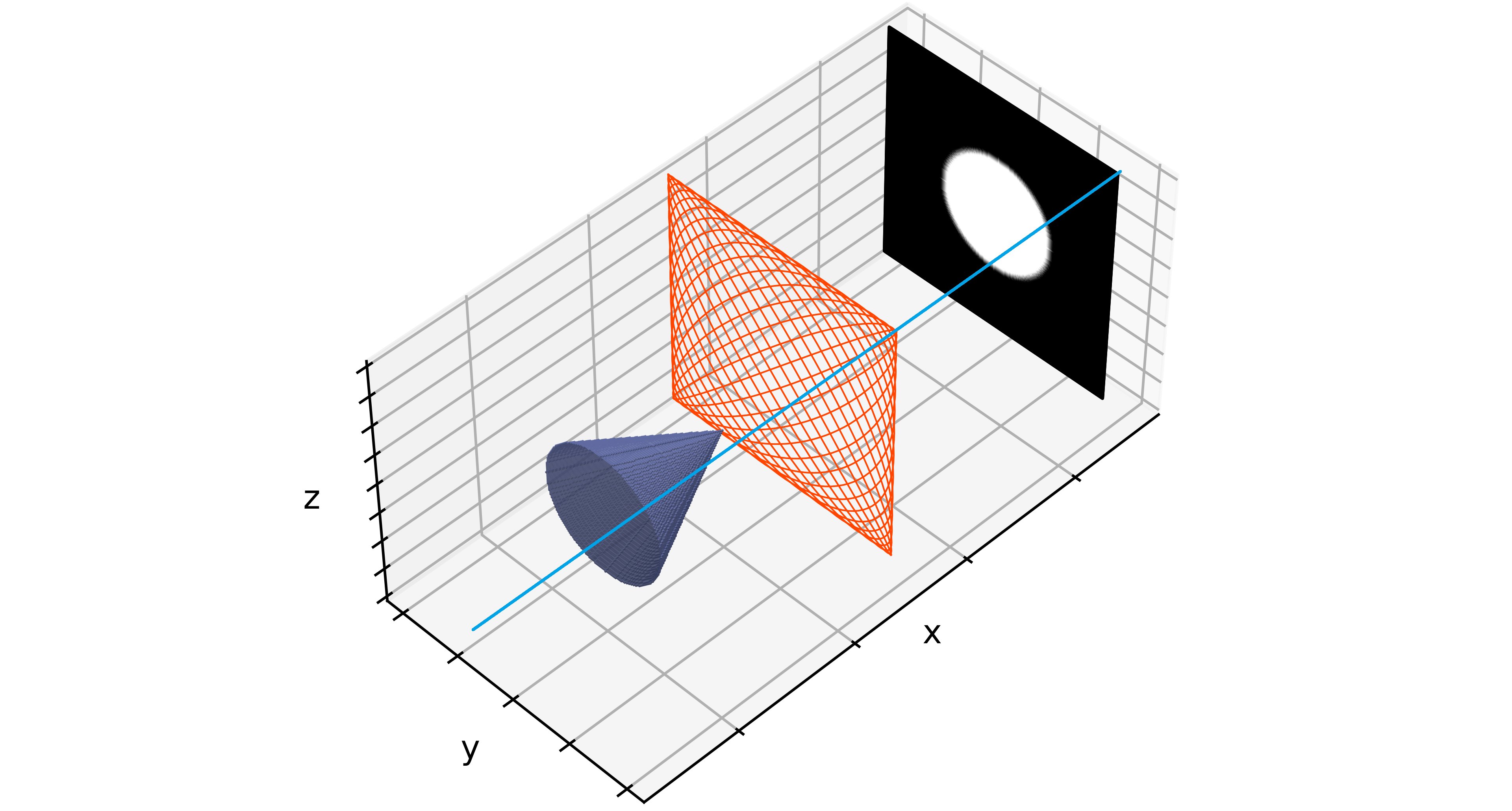
Fig. 1: A graphic representation of the components of the relation in Equation 19 for $\theta=0$. The conical particle distribution $\rho$ (in blue) is scanned moving the FFL (light blue) and the intersection point $\bm{r}(t)$ between the FFL and the $yz$-axis forms a Lissajous trajectory (in orange). The picture in black and white orthogonal to the $x$-axis is the X-Ray projection $X_{\theta}[\rho]$ for $\theta=0$.

3.3 Reconstruction formulae

In Equation 19 we have learned that the target distribution $\rho$ is linked to the signal $\bm{s}^{\theta}$ via the MPI Core Operator and consequently, the reconstruction of $\rho$ from the data must pass through the inversion of the MPI Core Operator. The inversion of the MPI Core Operator has been explored in [40], to which we refer the interested reader for a detailed discussion of the formulas and results presented in this section and in particular for a discussion on the ill-posedness of the inverse problem associated to the inversion. Before discussing further, we transform the data for every $\theta$ in a way such that the relationship in Equation 19 can be rewritten as the result of a direct application of the MPI Core Operator:

$$\tilde{\bm{s}}^{\theta}(t)=A_{h,\theta}\bigl{[}X_{\theta}[\rho]\bigr{]}\bigl{(}\bm{r}(t)\bigr{)}\bm{v}(t)\quad\text{with}\quad\tilde{\bm{s}}^{\theta}(t)=-\frac{1}{m\mu_{0}}E_{\theta}^{-1}P^{-1}\bm{s}^{\theta}.$$ (28)

The relation in Equation 28 is precisely of the form studied in [40] and it has been proven that the trace of the MPI Core Operator contains all the information needed for the reconstruction, i.e., if $\alpha_{h}[\rho](r)=\operatorname{trace}A_{h}[\rho]$ for some distribution $\rho$, then the trace is the convolution $\alpha_{h}[\rho](r)=(\rho*\kappa_{h})(r)$ between the distribution $\rho$ and the scalar valued kernel $\kappa_{h}$ having the following form in the general n-dimensional case:

$$\kappa_{h}(y)=\frac{1}{h}f\left(\frac{\lvert y\rvert}{h}\right),\quad\text{with}\quad f(z)=\mathcal{L}^{\prime}(z)+\mathcal{L}(z)\frac{n-1}{z}.$$ (29)

With these considerations we can state the first reconstruction formula:

Theorem 4 (First Reconstruction Formula).

Let $\theta\in[0,\pi)$ and $F(r)=A_{h,\theta}\bigl{[}X_{\theta}[\rho]\bigr{]}(r)$ be an ideal sampling of the MPI Core Operator each point $r$, then

$$X_{\theta}[\rho]=\kappa_{h}^{-1}\circ\operatorname{trace}\left(F\right),$$ (30)

where we denote with the symbol $\kappa_{h}^{-1}\circ$ the deconvolution w.r.t. the kernel $\kappa_{h}$.

Proof.

Let $\theta\in[0,\pi)$ be a scanning angle, the signal $\bm{s}^{\theta}(t)$ produced by a scan can be described according to 3 as in Equation 25. Applying the change of variables in Equation 28, we obtain that the relationship between $\tilde{\bm{s}}^{\theta}(t)$ and the X-Ray projection $X_{\theta}[\rho]$ can be written as follows:

$$\tilde{\bm{s}}^{\theta}(t)=\biggl{[}\int_{\mathbb{R}^{2}}X_{\theta}[\rho](\bm{y})\nabla_{\bm{r}}\biggl{(}\mathcal{L}\biggl{(}\frac{\lVert\bm{r}(t)-\bm{y}\rVert}{h}\biggr{)}\frac{\bm{r}(t)-\bm{y}}{\lVert\bm{r}(t)-\bm{y}\rVert}\biggr{)}\,d\bm{y}\biggr{]}\bm{v}(t),$$ (31)

with $\bm{r}(t)$ as in Equation 24, and $\bm{v}(t)=\frac{d}{dt}\bm{r}(t)$. In particular, $\bm{r}(t)$ as in Equation 24 is a 2D trajectory in the $yz$-plane (the first coordinate is always $0$), the X-Ray projection $X_{\theta}[\rho]$ is a distribution in 2 variables and the integral in Equation 31 is the 2D FFP MPI Core Operator as in Equation 26. This means that upon the change of variables, the modeling of the FFL 3D scan data is formally equivalent to the data obtained by performing a 2D FFP scan of the X-Ray projection as 2D distribution in the $yz$-plane. We can therefore apply [40, Theorem 3.5] for the ideal sampling $F(r)$ for $r\in\mathbb{R}^{2}$ for the distribution $X_{\theta}[\rho]$, which yields the reconstruction formula in Equation 30. ∎

Remark 1.

The first reconstruction formula in 4 involves a deconvolution wich has been proven to be ill-posed [40] and constitutes the first source of ill-posedness of the reconstruction algorithm in Section 4.

Applying the reconstruction formula in 4, one obtains a distribution $X_{\theta}$ in two variables on the plane orthogonal to the direction $\bm{e}_{\theta}$ for every angle $\theta$. In particular, we obtain the sheaf of all planes through the $z$-axis and on each one of these planes we have the X-Ray projection of the distribution $\rho$. The idea behind the second reconstruction formula comes from the observation that the X-Ray and Radon transforms coincide in 2D [42]: indeed, if we restrict ourselves to a plane orthogonal to the $z$-axis, for example on the plane $\mathbf{L}_{a}=\{(x,y,z)\in\mathbb{R}^{3}\colon z=a\}$ for some $a\in\mathbb{R}$, then the 2D Radon transform of angle $\theta$ on $\mathbf{L}_{a}$ coincides with the X-Ray transform of angle $\theta$ on $\mathbf{L}_{a}$ and we can consider the Filtered Back Projection (FBP) [42]: given a distribution $\rho$ and the set of its X-Ray projections $X_{\theta}[\rho]$ for all $\theta\in[0,\pi)$, the following formula holds true for every $a\in\mathbb{R}$:

$$\rho(\bm{x})\biggl{\lvert}_{\mathbf{L}_{a}}=\frac{1}{2\pi}\int_{0}^{\pi}\left(X_{\theta}[\rho]\biggl{\lvert}_{\mathbf{L}_{a}}*\,h\right)\bigl{(}\langle\bm{x},\,\bm{e}_{\theta}\rangle\bigr{)}\,d\theta,$$ (32)

where $\bm{x}=(x,y,a)^{T}$, $\bm{e}_{\theta}=(\cos\theta,\sin\theta,a)$ and $h$ is the kernel whose Fourier transform is $\mathcal{F}(h)(\omega)=\lvert\omega\rvert$. With Equation 32 we can formulate our second reconstruction formula, which is an inversion of the relation in Equation 32 passing through the Fourier space and employing a window function for noise filtering:

Theorem 5 (Second Reconstruction Formula).

Given a 3D distribution $\rho$ and the set of all of its X-Ray projections $X_{\theta}[\rho]$ for all $\theta\in[0,\pi)$ around the $z$-axis, then the following equality holds true for every restriction of $\rho$ on the plane $\mathbf{L}_{a}$ with $a\in\mathbb{R}$:

$$\rho(\bm{x})\biggl{\lvert}_{\mathbf{L}_{a}}=\int_{0}^{\pi}\mathcal{F}^{-1}\left(\mathcal{F}\biggl{(}X_{\theta}[\rho]\biggl{\lvert}_{\mathbf{L}_{a}}\biggr{)}(\omega)\cdot\lvert\omega\rvert\cdot w(\lvert\omega\rvert)\right)\,d\theta$$ (33)

for some window function $w$.

Proof.

Given $\mathbf{L}_{a}=\{(x,y,z)\in\mathbb{R}^{3}\colon z=a\}$ for some $a\in\mathbb{R}$, the restriction of the X-Ray projections $X_{\theta}[\rho]$ onto $\mathbf{L}_{a}$ is the 2D Radon transform in the direction $\bm{e}_{\theta}=(\cos\theta\,,\sin\theta)^{T}$ of the 2D distribution $\rho(\bm{x})\bigl{\lvert}_{\mathbf{L}_{a}}$. The X-Ray projections lay on the planes $\mathbf{L}_{\theta}$ forming a sheaf around the $z$-axis, meaning that the set of restrictions $X_{\theta}[\rho]\bigl{\lvert}_{\mathbf{L}_{a}}$ for $\theta\in[0,\pi)$ form a complete set of 2D Radon transforms for all directions and the Radon inversion formula in [42, Theorem 2.1] holds true (for the Riesz potential $I^{\alpha}$ with $\alpha=0$), i.e., Equation 32 with $h$ the kernel whose Fourier transform is $\mathcal{F}(h)(\omega)=\lvert\omega\rvert$ holds true for every $\mathbf{L}_{a}$. Retrieving the restrictions $\rho(\bm{x})\bigl{\lvert}_{\mathbf{L}_{a}}$ is therefore a problem treatable by performing a deconvolution of the convolution product in the integrand in Equation 32. We perform the deconvolution using a filter in frequency space. Equation 33 describes precisely the frequency filtering, by first applying the Fourier transform, multiplying the frequencies by some filter $w$ and transforming back the filtered Fourier spectrum into the space domain. ∎

4 Reconstruction algorithm

In this section we describe the discrete data, and we formulate the reconstruction algorithm, which can be subdivided into three mains steps: (i) reconstruction of the MPI Core Operators from the scan data for each angle; (ii) regularized deconvolution of the traces of the MPI Core Operators reconstructed in the first step; (iii) reconstruction of the 3D distribution using the reconstruction formula in 5.

First, we describe the discretization employed for both the simulation of the experiments and the reconstruction algorithm: we consider a 3D particle distribution $\rho\colon\mathbb{R}^{3}\to\mathbb{R}^{+}$ such that $\mathrm{supp}(\rho)$ is compactly contained in the scanning domain $\Omega=[x_{1},x_{2}]\times[y_{1},y_{2}]\times[z_{1},z_{2}]$. This domain is discretized considering an $N_{x}\times N_{y}\times N_{z}$ grid and identifying the $(i,j,k)$-th cell of the grid with its center $(x_{i},y_{j},z_{k})$ defined as follows:

$$\begin{split}x_{i}&=x_{1}+\left(0.5+i\right)\Delta x,\quad\text{where}\quad\Delta x=(x_{2}-x_{1})/N_{x}\text{ and }i=0,\cdots,N_{x}-1\\ y_{j}&=y_{1}+\left(0.5+j\right)\Delta y,\quad\text{where}\quad\Delta y=(y_{2}-y_{1})/N_{y}\text{ and }j=0,\cdots,N_{y}-1\\ z_{k}&=z_{1}+\left(0.5+k\right)\Delta z,\quad\text{where}\quad\Delta z=(z_{2}-z_{1})/N_{z}\text{ and }k=0,\cdots,N_{z}-1.\\ \end{split}$$ (34)

For the acquisition of the scans, we consider the angles $\theta$ in some set of angles $\Theta$, usually $\theta_{l}=l\cdot\frac{\pi}{\lvert\Theta\rvert}$ where $l=0,\dots,\lvert\Theta\rvert-1$ and $\lvert\Theta\rvert\in\mathbb{N}$ is the total number of angles considered. For each angle $\theta_{l}$ we consider an acquisition time $T_{l}>0$ of the scan and we discretize the time considering equidistant points $t_{m}=m\cdot\frac{T_{m}}{L_{l}}$ for $m=0,\dots,L_{l}-1$ and $L_{l}$ is the number of time points of the scan performed with angle $\theta_{l}$. With the discretization of time we obtain a discretization of the scanning trajectories as in Equation 24, $\bm{r}_{m}=\bm{r}(t_{m})$, the velocities $\bm{v}_{m}=\bm{v}(t_{m})$ and of the signal $\bm{s}_{m}^{\theta_{l}}=\bm{s}^{\theta_{l}}(t_{m})$ for every $m=0,\dots,L_{l}-1$ and $l=0,\dots,\lvert\Theta\rvert-1$. The task of the reconstruction algorithm is to reconstruct a discrete version of the distribution from the data, i.e., to obtain a discrete distribution $\rho_{\mathrm{rec}}\in\mathbb{R}^{N_{x}\times N_{y}\times N_{z}}$ with an algorithm in three steps which we now describe in detail.

First Stage: Obtain the Trace of the MPI Core Operator from the Data

In this first stage we aim at reconstructing the MPI Core Operators from the raw data, which for each $\theta_{l}\in\Theta$ consists of the set of triples $\{(\bm{s}^{\theta_{l}}_{m},\bm{r}_{m},\bm{v}_{m})\colon m=0,\dots,L_{l}-1\}$. We transform the data points according to Equation 28, such that they are all in the same frame of reference. In particular, the problem for each angle is of the form $\bm{s}=A(\bm{r})\bm{v}$, where $A(\bm{r})\in\mathbb{R}^{2\times 2}$ is a shorthand notation for the discrete matrix-valued field $A_{j,k}\in\mathbb{R}^{2\times 2\times N_{y}\times N_{z}}$ evaluated at the point $\bm{r}$ and which discretizes the MPI Core Operator $A_{h,\theta}$; here $N_{y}\times N_{z}$ is the discretization of the transformed region of interest $[y_{1},y_{2}]\times[z_{1},z_{2}]$, which upon the transformation in Equation 28 is the same for each angle. To solve this problem we choose to employ the Local Least Squares (LLSq) method [40], i.e., given an angle $\theta$, for each cell $C_{j,k}$ of the $N_{y}\times N_{z}$ grid we collect into a matrix $V_{j,k}$ in a column-wise fashion all those velocities $\bm{v}_{m}$ for which the relative position $\bm{r}_{m}$ falls into the cell $C_{j,k}$; analogously, if $\bm{r}_{m}\in C_{j,k}$ then we add $\bm{s}^{\theta_{l}}_{m}$ in column-wise fashion to a matrix $S_{j,k}$ and we form the following $N_{y}\times N_{z}$ matrix problems for each cell of the grid:

$$S_{j,k}=A_{j,k}(y_{j},z_{k})V_{j,k},$$ (35)

where the discrete reconstruction of the MPI Core Operator $A_{j,k}$. The problems in Equation 35 can be solved in a least square fashion using the QR decomposition of $V_{j,k}$ (for a more detailed discussion about when the problems are well defined and further details about their solution we refer the interested reader to [40]). Once all $N_{y}\times N_{z}$ problems of the form in Equation 35 has been solved, the discrete field $u_{j,k}=\operatorname{trace}A_{j,k}$ of the traces of the reconstructed MPI Core Operator serves as input for the second stage.

Second Stage: Reconstruction of the X-Ray Projections from the Traces

The input of this stage are the trace fields $u^{l}$ for each angle $\theta_{l}\in\Theta$. From these trace fields it is possible to retrieve the X-Ray transforms of the distribution using the First Reconstruction Formula in 4. In particular, for each angle $\theta_{l}$ we solve the deconvolution problem in Equation 30 of the trace field $u^{l}$ and the kernel $\kappa_{h}$ in Equation 29 to obtain $\chi_{l}\coloneq X_{\theta_{l}}[\rho]$. Because of course the data $\bm{s}^{\theta_{l}}$ and hence $u^{l}$ is corrupted by noise, the deconvolution problems are severely ill-posed and regularization is needed. Following [40] we employ the Tikhonov regularization technique with a smoothing regularizer (smoothness of the solution has been proven in [40]) and we formulate the following (continuous) minimization problem:

$$\chi_{l}=\arg\min_{\hat{\chi}}\lambda_{l}\left\lVert\nabla_{r}\hat{\chi}\right\rVert_{L^{2}}^{2}+\left\lVert\kappa_{h}*\hat{\chi}-u^{l}\right\rVert_{L^{2}}^{2},$$ (36)

with regularization parameters $\lambda_{l}>0$.

Of the problem in Equation 36 we consider the same discretization as in the first stage, i.e., for each angle $\theta_{l}$ we reconstruct a discretized version $(\chi_{l})_{j,k}\in\mathbb{R}^{N_{y}\times N_{z}}$ of the X-Ray projections. To this aim we consider a discretization on the $N_{y}\times N_{z}$ grid of the $\kappa_{h}$ (with the midpoint rule) and denote with $K_{h}$ the matrix representing the convolution with $\kappa_{h}$. If moreover, $D$ is the matrix representing the discratization of the gradient with forward differences, we obtain the following discrete version of the problem:

$$\chi_{l}=\arg\min_{\hat{\chi}}\lambda_{l}\left\lVert D\hat{\chi}\right\rVert_{2}^{2}+\left\lVert K_{h}\hat{\chi}-u^{l}\right\rVert_{2}^{2},$$ (37)

which can be solved by considering the corresponding Euler-Lagrange equations

$$-\lambda_{l}L\chi_{l}+K_{h}^{T}\left(K_{h}\chi_{l}-u^{l}\right)=0$$ (38)

where $-L=D^{T}D$ is the negative Laplacian with zero Dirichlet boundary conditions.

Third Stage: Radon Inversion of the X-Ray Sinograms

Given the reconstruction of the X-Ray projections $X_{\theta_{l}}[\rho]=\chi_{l}$ in the second stage, we finally reconstruct the distribution. The idea is to proceed slice-wise along the $z$-axis using FBP as in 5. In particular, we consider the planes $\mathbf{M}_{k}\coloneq\{(x,y,z)\in\mathbb{R}^{3}\colon z=z_{k}\}$ with $z_{k}$ as in Equation 34 and we obtain the $k$-th slice of $\rho_{\mathrm{rec}}$ using Equation 33, i.e.,

$$\rho_{\mathrm{rec}}(\bm{x})\bigl{\lvert}_{\mathbf{M}_{k}}=\frac{\pi}{\lvert\Theta\rvert}\sum_{l=0}^{\lvert\Theta\rvert-1}\mathcal{F}^{-1}\left(\mathcal{F}\biggl{(}\chi_{l}\bigl{\lvert}_{\mathbf{M}_{z}}\biggr{)}(\omega)\cdot\lvert\omega\rvert\cdot w(\lvert\omega\rvert)\right)(\bm{x})$$ (39)

for some window function $w$. A pseudocode of the complete three-stage algorithm can be found in Algorithm 1.

Algorithm 1 Proposed three-stage model-based reconstruction algorithm for 3D Field-Free Line Magnetic Particle Imaging

Input: A set of scanning angles $\Theta$ and a domain 3D $\Omega$; for each $\theta\in\Theta$, time independent samples $\bm{s}_{\theta}^{\theta}=\bm{s}^{\theta}(t_{m})$, functions $\Lambda_{1}$,$\Lambda_{2}$, gradient strength $G$ and amplitudes $A_{1}$, $A_{2}$ and a regularization parameters $\lambda_{l}>0$ for $l=0,\dots,\lvert\Theta\rvert-1$.
Output: Reconstructed 3D particle density $\rho_{\mathrm{rec}}$.

Initialize $\rho$ given the grid on $\Omega$;

Initialize scanning positions $\bm{r}_{m}\leftarrow\left(\frac{A_{1}\Lambda_{1}(t_{m})}{G}\,,\frac{A_{2}\Lambda_{2}(t_{m})}{G}\right)$ and $\bm{v}_{m}=\frac{d}{dt}\bm{r}_{m}$;

for $\theta$ in $\Theta$ do

     $l\leftarrow$ index of $\theta$;

     Transform $\bm{s}_{m}^{\theta}\leftarrow\tilde{\bm{s}}^{\theta}(t_{m})$ as in Equation 28;

     \\First stage: obtain the traces of the X-Ray projections.

     Associate $\bm{s}_{m}^{\theta}$ with cell $C_{j,k}$ if $\bm{r}_{m}\in C_{j,k}$.

     for each cell $C_{j,k}$ do

         Form the matrices $V_{j,k}$ and $S_{j,k}$;

         Solve equation $S_{j,k}=A_{j,k}(y_{j},z_{k})V_{j,k}$ with $QR$ decomposition;

         Update $(A^{l})_{j,k}\leftarrow A_{j,k}(y_{j},z_{k})$;

     end for

     Get the traces $u^{l}\leftarrow\operatorname{trace}(A^{l})$;

     \\Second stage: obtain the X-Ray projections solving Eq. (37).

     Update $\chi_{l}\leftarrow\mathrm{ConjugatedGradient}(-\lambda_{l}L+K_{h}^{T}K_{h}\,,K_{h}^{T}u^{l})$;

end for

\\Third stage: reconstruct $\rho$ in a slice-wise fashion.

for $k\leftarrow 0$ to $N_{z}-1$ do

     Update $\rho_{\mathrm{rec}}(\bm{x})\bigl{\lvert}_{\mathbf{M}_{k}}$ using Equation 39;

end forreturn The reconstruction $\rho_{\mathrm{rec}}$.

5 Numerical Experiment

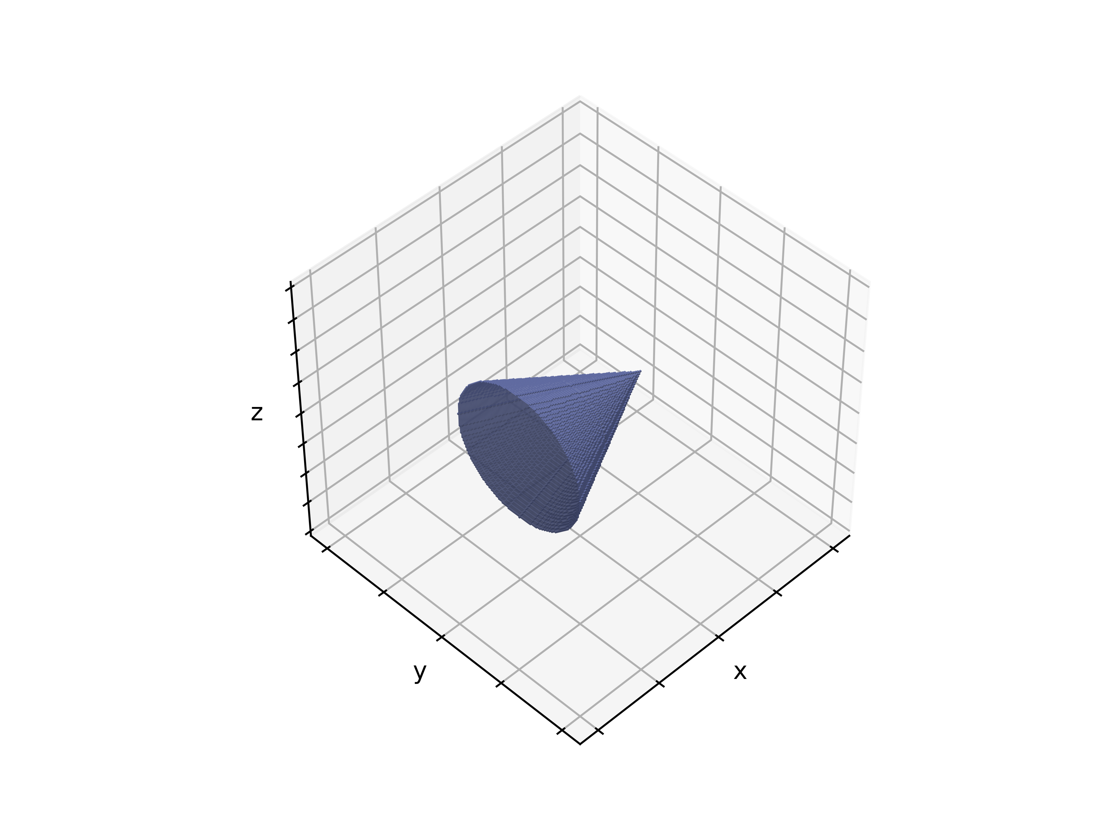
Fig. 2: The 3D phantom used in the experiment: it is a cone with the center of its circular base and the apex collinear on the $x$-axis.

In this section we describe a numerical experiment to demonstrate the potential of the reconstruction algorithm in Section 4 for a simulated 3D FFL scan.

Experimental Setup and Simulation of the Scans

We consider the cone shaped 3D distribution $\rho_{\mathrm{GT}}$ (visualized in Figure 2) which has been produced in the domain $\Omega=[-1,1]^{3}$ and $\Omega$ has been discretized with a $N_{x}\times N_{y}\times N_{z}=200\times 200\times 200$ grid. We have simulated a 3D FFL scan applying magnetic fields as in Equation 13 with sinusoidal functions $\Lambda_{i}=\cos(2\pi f_{i}t+\phi_{i})$ for $i=1,2$, where $f_{i}$ are integer frequencies. In particular, the shifts have been chosen to be $\phi_{1}=\phi_{2}=\pi/2$, the frequencies to be $f_{1}=201$, $f_{2}=202$ and their amplitudes in Equation 13 to be $A_{1}=A_{2}=1$. For the simulation of the signal $\bm{s}^{\theta}$ we have used the relationship in Equation 19 with a trivial coil sensitivity pattern and gradient strength $P=\mathrm{Id}_{3}$ the identity matrix, $G=1$, magnetic moment $m=1$, the resolution parameter $h=10^{-2}$ and the known value of $\mu_{0}=1.25663706212\cdot 10^{-6}$. We consider scans with $200$ equidistant angles $\theta_{l}=l\cdot\frac{\pi}{200}$ for $l=0,\dots,199$ and for each angle $\theta_{l}$ we have considered $L=400\,000$ time samples $t_{m}=m\cdot\frac{T}{L}$ for $m=0,\dots,L-1$, assuming $T=1$ for each angle.

To account for noise contamination, we have corrupted the simulated signals with $10\%$ additive Gaussian noise, i.e., for each angle $\theta$ we considered a corrupted signal

$$\hat{\bm{s}}^{\theta}(t_{m})=\bm{s}^{\theta}(t_{m})+\varepsilon_{\theta}N_{m}^{\theta}\quad\theta\in\left\{l\cdot\frac{\pi}{200}\colon l=0,\dots,199\right\}.$$ (40)

Here $N_{m}^{\theta}$ are i.i.d. random variables extracted from a normal distribution with zero mean and standard deviation of one. The noise amplitude in this case is

$$\varepsilon_{\theta}=0.1\cdot\max_{m}\{\lvert\bm{s}^{\theta}(t_{m})\rvert\}.$$ (41)

The signal in Equation 40 serves as input of the reconstruction algorithm in Section 4.

Reconstruction Parameters

The reconstruction has been performed considering $200\times 200\times 200$ grid cells as well. In particular, for every angle $\theta_{l}$ we have reconstructed the trace of the MPI Core Operator $u_{l}$ with the LLSq method as described in Section 4 on a $200\times 200$ grid. Each of these traces $u_{l}$ have been deconvolved by solving with the CG method the Euler-Lagrange equations associated to the deconvolution problem in Equation 38, with parameter $\lambda=\lambda_{l}=5\times 10^{-4}$ equal for all angles and fine tuned by hand. The maximum number of iterations for the CG algorithm in the first stage has been set to $1000$, if a relative tolerance of $10^{-10}$ has not been reached. The set of reconstructed X-Ray projections $\chi_{l}$ serves as the input for the third and last stage, where we employ the FBP formula in Equation 38 on each slice perpendicular to the $z$-axis, with the Ramp-filter $w(x)=x$ if $x\leq 0.5$ and $w(x)=0$ otherwise.

The algorithm described in the paper and the data simulation have been implemented in Python 3.9, using the packages Numpy, SciPy, Scikit-image and PyTorch. The numerical experiments were performed on a desktop computer with 13th Gen Intel(R) Core(TM) i9-13900KS, 128 GB of RAM, an NVIDIA RTX A6000 GPU and Windows 11 Pro.

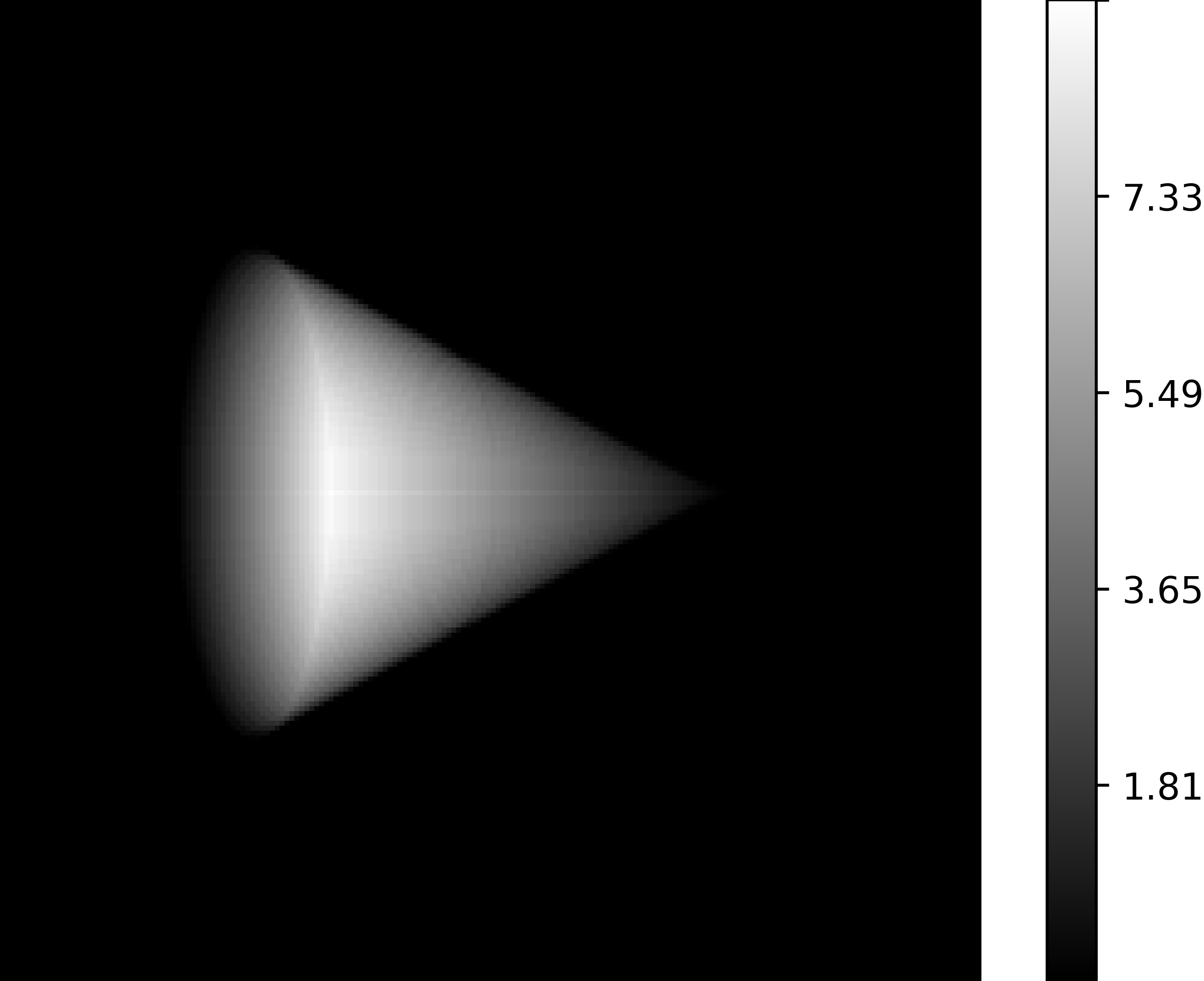
(a) X-Ray Projection $X_{72^{\circ}}[\rho_{\mathrm{GT}}]$

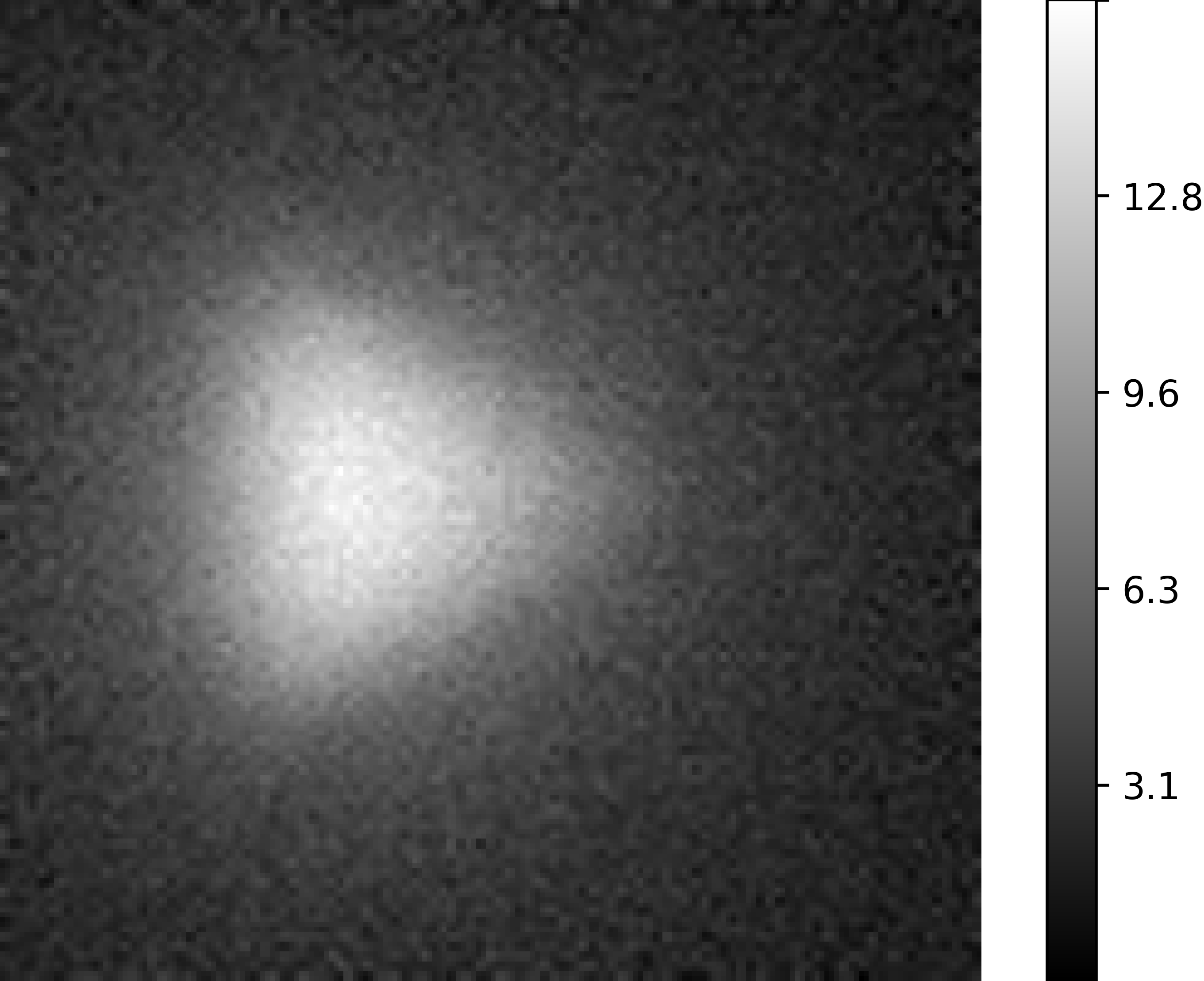
(b) Reconstructed Trace $u$.

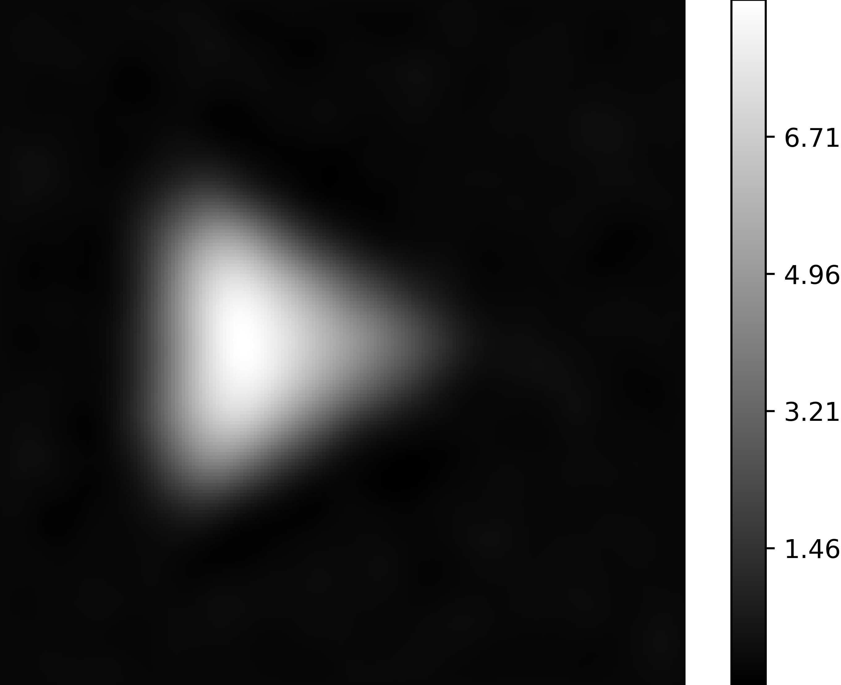
(c) Reconstructed Projection $\chi$.

(d) Plot of the three components of the signal $\bm{s}^{\theta}(t_{m})$ with $\theta=72^{\circ}$ (from top to bottom the $x$,$y$ and $z$ components).

Fig. 3: Example of the first two stages of the reconstruction algorithm for the scan performed at angle $\theta=72^{\circ}$.

(a) $\rho_{\mathrm{GT}}$ slice, $x=-0.505$

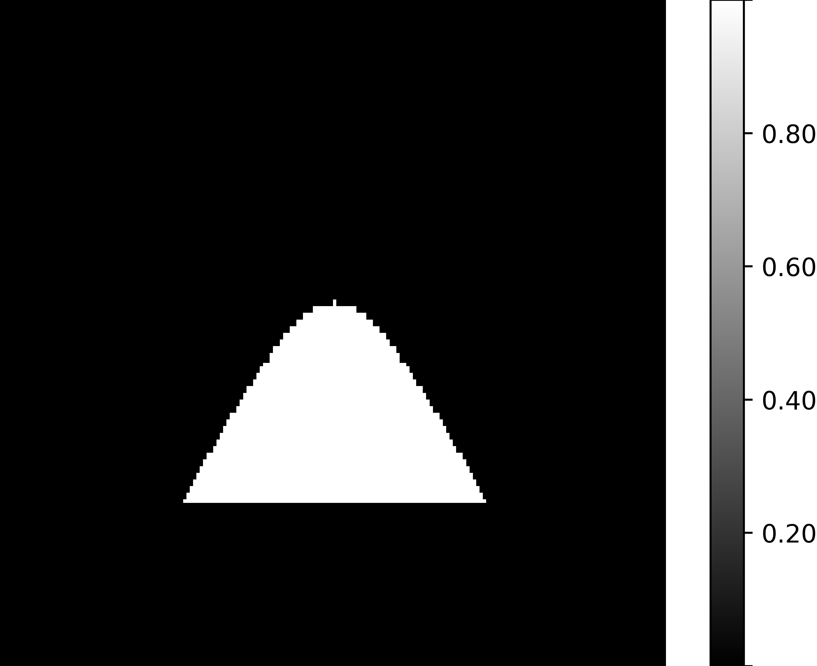
(b) $\rho_{\mathrm{GT}}$ slice, $y=-0.195$

(c) $\rho_{\mathrm{GT}}$ slice, $z=-0.005$

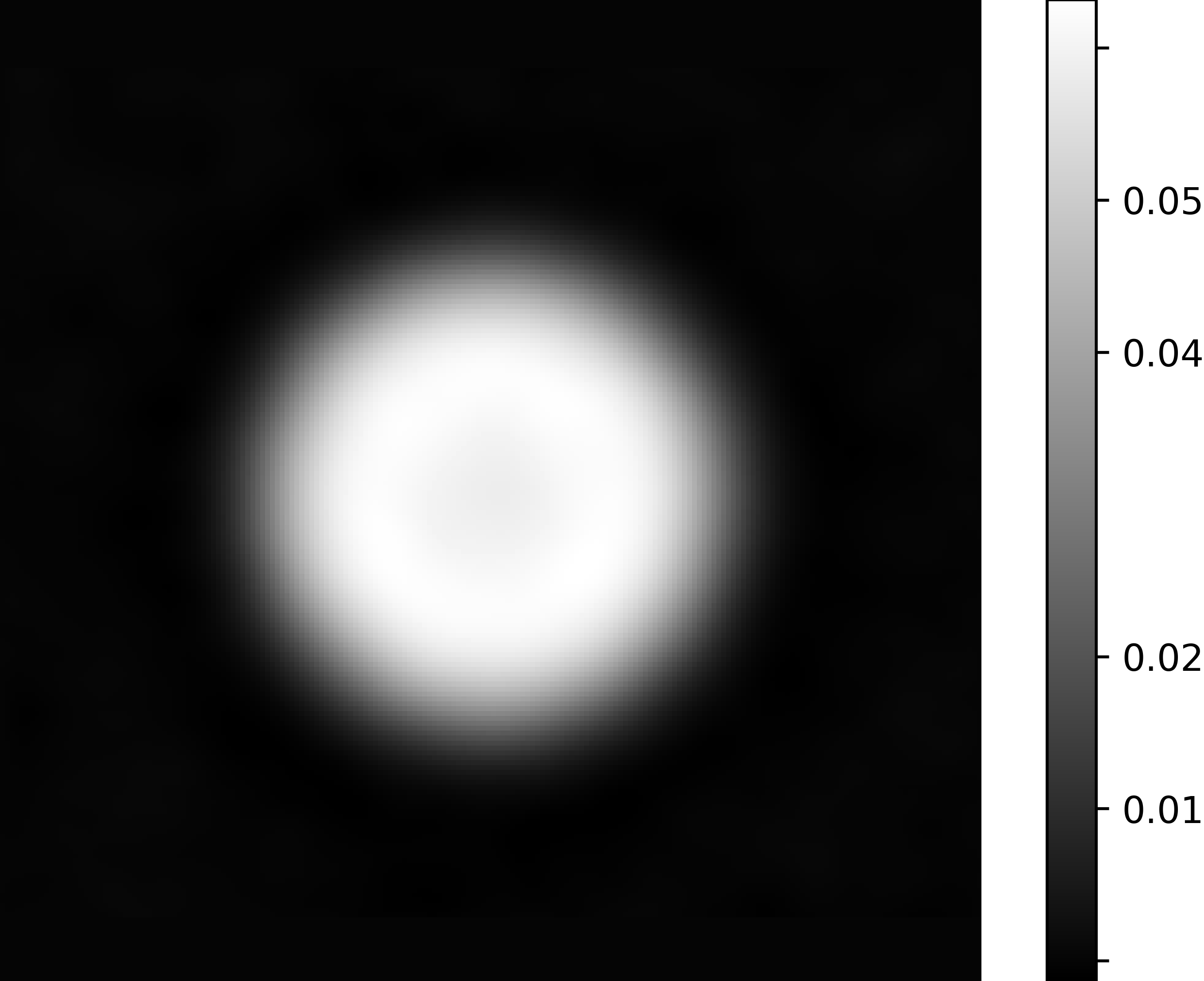
(d) $\rho_{\mathrm{rec}}$ slice, $x=-0.505$

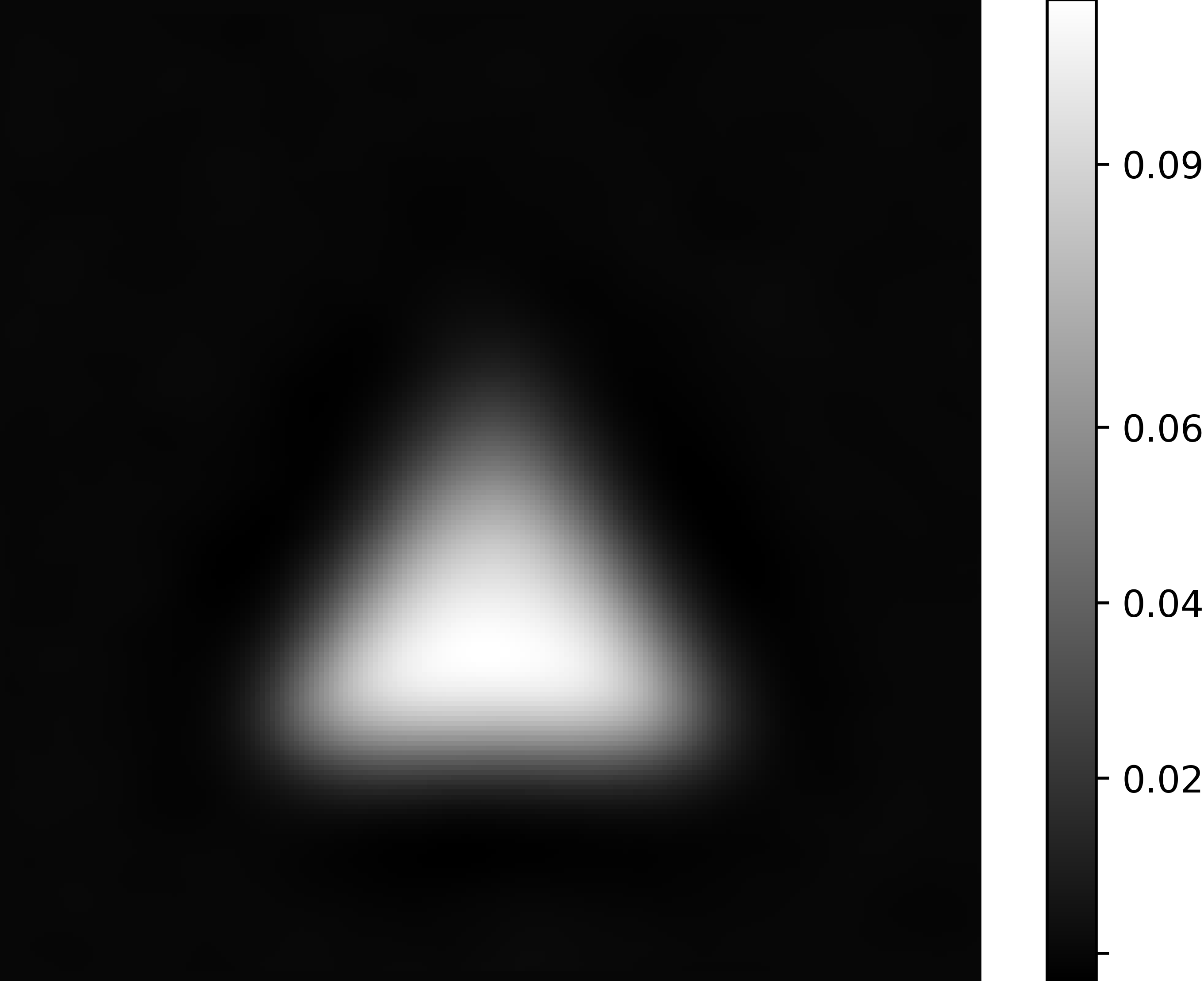
(e) $\rho_{\mathrm{rec}}$ slice, $y=-0.195$

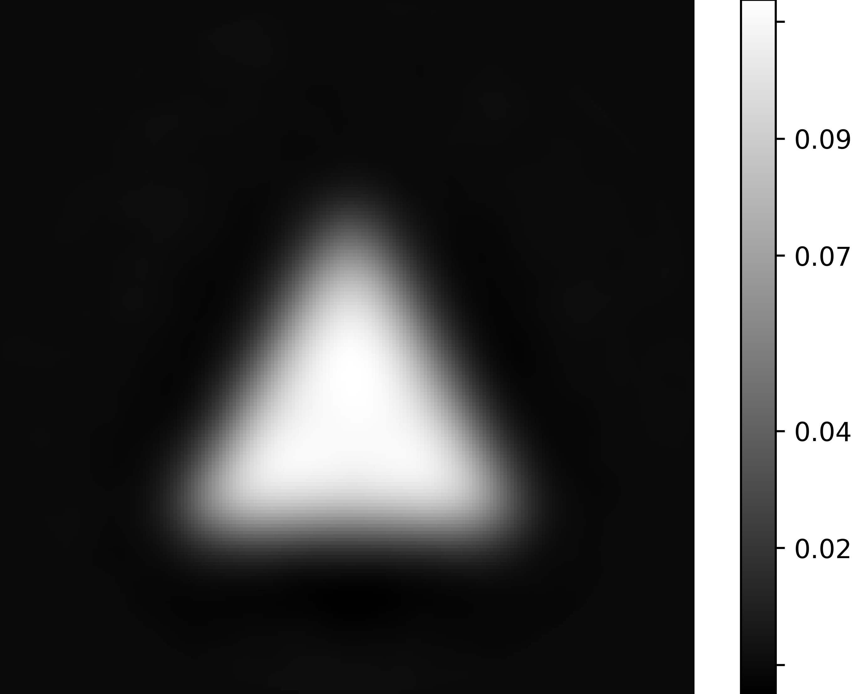
(f) $\rho_{\mathrm{rec}}$ slice, $z=-0.005$

(g) $\rho_{\mathrm{GT}}$

(h) $\rho_{\mathrm{rec}}$

Fig. 4: Reconstruction of a cone shaped phantom with the 3D FFL scan proposed and the three stage algorithm. In Figure 4(g) the ground truth $\rho_{\mathrm{rec}}$ and in Fig. 4(h) the boolean plot of the 3D reconstruction. In Figures 4(a), 4(b) and 4(c) are shown three slices of $\rho_{\mathrm{GT}}$ along each of the three axis. In Figures 4(d), 4(e) and 4(f) are shown exactly the same slices of the reconstruction $\rho_{\mathrm{rec}}$. We observe that the reconstruction algorithm is capable of reconstructing the core features of the distribution.

Discussion of the Results

In Figure 3 we can see an example of the reconstructions of the X-Ray projections with the first two stages of the algorithm presented in this paper: a reconstruction from the signal in Figure 3(d), obtained from the scan performed at angle $\theta=72^{\circ}$. In particular, in Figures 3(b) and 3(c) we can see the reconstructions of the trace $u$ of the MPI Core Operator and the reconstruction after the deconvolution step, respectively. In Figure 4 we can see the final reconstruction after the third stage of the algorithm (the Radon inversion). The reconstructed distribution is plotted in boolean values in Figure 4(h), where we put all values below $5\%$ of $\max\{\lvert\rho_{\mathrm{rec}}\rvert\}$ to 0 and all the others to 1. For a fairer comparison between the $\rho_{\mathrm{GT}}$ and $\rho_{\mathrm{rec}}$ we have also plotted random examples of slices of the two 3D distribution along each of the axes. In particular, Figures 4(a), 4(b) and 4(c) are three slices of $\rho_{\mathrm{GT}}$ along the $x$,$y$ and $z$-axis respectively. The exact same slices of $\rho_{\mathrm{rec}}$ can be seen in Figures 4(d), 4(e) and 4(f). Comparing the ground truth and the reconstruction it is evident that the main algorithm is capable of reconstructing shapes, but the edges of the reconstruction are smoothed out. This smoothing out of the reconstruction can be already seen in the reconstructed X-Ray projections, for example in Figure 3(c). This is due to the fact that indeed the regularizer (see Equation 36) employed in the second stage enforces smoothness of the reconstruction and could be mitigated employing regularizers that are more suitable for the reconstruction of edges (more details in Section 6). Finally, this experiment demonstrates that a model-based reconstruction of 3D distributions from 3D FFL scans using our algorithm and methodology is promising.

6 Conclusions

In this work we have provided model-based reconstruction formulae for 3D FFL MPI that relate the signal obtained in the receiving coils to the target distribution via the MPI Core Operator and the X-Ray projection. Based on those, as our second contribution we have proposed a three stage reconstruction algorithm: for each angle, the first two stages are employed to first reconstruct the traces of the MPI Core Operators involved and then, to reconstruct the X-Ray projections of the ground truth. In the third stage, the whole 3D distribution is reconstructed using the Fourier Slice Theorem. Finally, we have demonstrated the applicability of the proposed algorithm with a simulated numerical example. Directions of future work include the development and testing of tools for the enhancement of each of the three stages of the algorithm presented, for example methods that encourage sparsity of the reconstruction and enforce positivity [16] and methods that have better edge preserving properties, like TV type regularizers [47] as well as Potts type regularizers [62, 53, 63]. Another important direction of research is the application of the algorithm to real data. It is known that the LFVs in the FFL acquisition topology are not ideal lines and rather resemble 3-dimensional banana-shaped cylinders [7]. In order to counteract artifacts coming from the assumption of ideal FFLs, work should be also done to incorporate existing more realistic models [7] into the stages of the algorithms here presented.

References

- [1] H. Arami, E. Teeman, A. Troksa, H. Bradshaw, K. Saatchi, A. Tomitaka, S. S. Gambhir, U. O. Häfeli, D. Liggitt, and K. M. Krishnan, Tomographic Magnetic Particle Imaging of Cancer Targeted Nanoparticles, Nanoscale, 9 (2017), pp. 18723–18730.
- [2] A. C. Bakenecker, M. Ahlborg, C. Debbeler, C. Kaethner, T. M. Buzug, and K. Lüdtke-Buzug, Magnetic Particle Imaging in Vascular Medicine, Innovative Surgical Sciences, 3 (2018), pp. 179–192.
- [3] K. Bente, M. Weber, M. Graeser, T. F. Sattel, M. Erbe, and T. M. Buzug, Electronic Field Free Line Rotation and Relaxation Deconvolution in Magnetic Particle Imaging, IEEE Transactions on Medical Imaging, 34 (2015), pp. 644–651.
- [4] M. Bertero, P. Boccacci, and C. De Mol, Introduction to Inverse Problems in Imaging, CRC press, 2021.
- [5] C. Billings, M. Langley, G. Warrington, F. Mashali, and J. A. Johnson, Magnetic Particle Imaging: Current and Future Applications, Magnetic Nanoparticle Synthesis Methods and Safety Measures, International Journal of Molecular Sciences, 22 (2021).
- [6] G. Bringout, Field Free Line Magnetic Particle Imaging Characterisation and Imaging Device Up-Scaling, PhD thesis, Universität zu Lübeck, Oct. 2016.
- [7] G. Bringout, W. Erb, and J. Frikel, A new 3D Model for Magnetic Particle Imaging Using Realistic Magnetic Field Topologies for Algebraic Reconstruction, Inverse Problems, 36 (2020), p. 124002.
- [8] T. M. Buzug, Computed Tomography From Photon Statistics to Modern Cone-Beam CT, Springer, Germany, 2008.
- [9] S. Chikazumi and S. Charap, Physics of Magnetism, Krieger Publishing, New York, 1978.
- [10] S.-M. Choi, J.-C. Jeong, J. Kim, E.-G. Lim, C.-B. Kim, S.-J. Park, D.-Y. Song, H.-J. Krause, H. Hong, and I. S. Kweon, A Novel Three-Dimensional Magnetic Particle Imaging System Based on the Frequency Mixing for the Point-of-Care Diagnostics, Scientific Reports, 10 (2020), p. 11833.
- [11] J. J. Connell, P. S. Patrick, Y. Yu, M. F. Lythgoe, and T. L. Kalber, Advanced Cell Therapies: Targeting, Tracking and Actuation of Cells with Magnetic Particles, Regenerative medicine, 10 (2015), pp. 757–72.
- [12] Y. Du, X. Liu, Q. Liang, X.-J. Liang, and J. Tian, Optimization and Design of Magnetic Ferrite Nanoparticles with Uniform Tumor Distribution for Highly Sensitive MRI/MPI Performance and Improved Magnetic Hyperthermia Therapy, Nano Letters, 19 (2019), pp. 3618–3626.
- [13] M. Erbe, Field Free Line Magnetic Particle Imaging, Springer, 01 2014.
- [14] J. Franke, N. Baxan, H. Lehr, U. Heinen, S. Reinartz, J. Schnorr, M. Heidenreich, F. Kiessling, and V. Schulz, Hybrid MPI-MRI System for Dual-Modal In Situ Cardiovascular Assessments of Real-Time 3D Blood Flow Quantification - A Pre-Clinical In Vivo Feasibility Investigation, IEEE Transactions on Medical Imaging, 39 (2020), pp. 4335–4345.
- [15] V. Gapyak, T. März, and A. Weinmann, Quality-Enhancing Techniques for Model-Based Reconstruction in Magnetic Particle Imaging, Mathematics, 10 (2022).
- [16] V. Gapyak, T. März, and A. Weinmann, Variational Model-Based Reconstruction Techniques for Multi-Patch Data in Magnetic Particle Imaging, 2023, Submitted to Journal of Computational and Applied Mathematics (in Revision).
- [17] B. Gleich and J. Weizenecker, Tomographic Imaging Using the Nonlinear Response of Magnetic Particles, Nature, 435 (2005), pp. 1214–1217.
- [18] P. Goodwill and S. M. Conolly, The X-Space Formulation of the Magnetic Particle Imaging Process: 1-D Signal, Resolution, Bandwidth, SNR, SAR, and Magnetostimulation, IEEE Trans. Med. Imaging, 29 (2010), pp. 1851–1859.
- [19] , Multidimensional X-Space Magnetic Particle Imaging, IEEE Trans. Med. Imaging, 30 (2011), pp. 1581–1590.
- [20] P. W. Goodwill, J. J. Konkle, B. Zheng, E. U. Saritas, and S. M. Conolly, Projection X-Space Magnetic Particle Imaging, IEEE Trans Med Imaging, 31 (2012), pp. 1076–1085.
- [21] M. Graeser, F. Thieben, P. Szwargulski, F. Werner, N. Gdaniec, M. Boberg, F. Griese, M. Möddel, P. Ludewig, D. van de Ven, O. M. Weber, O. Woywode, B. Gleich, and T. Knopp, Human-Sized Magnetic Particle Imaging for Brain Applications, Nature Communications, 10 (2019), p. 1936.
- [22] J. Haegele, J. Rahmer, B. Gleich, J. Borgert, H. Wojtczyk, N. Panagiotopoulos, T. M. Buzug, J. Barkhausen, and F. M. Vogt, Magnetic Particle Imaging: Visualization of Instruments for Cardiovascular Intervention, Radiology, 265 (2012), pp. 933–938. PMID: 22996744.
- [23] S. Helgason, Integral Geometry and Radon Transforms, Springer New York, 2011.
- [24] S. Ilbey, C. B. Top, A. Güngör, T. Çukur, E. U. Saritas, and H. E. Guven, Comparison of System-Matrix-Based and Projection-Based Reconstructions for Field Free Line Magnetic Particle Imaging, Int J Mag Part Imag, 3 (2017).
- [25] J. D. Jackson, Classical Electrodynamics, Wiley, New York, NY, 3rd ed. ed., 1999.
- [26] D. Jiles, Introduction to Magnetism and Magnetic Materials, CRC press, 1998.
- [27] K. O. Jung, H. Jo, J. H. Yu, S. S. Gambhir, and G. Pratx, Development and MPI Tracking of Novel Hypoxia-Targeted Theranostic Exosomes, Biomaterials, 177 (2018), pp. 139–148.
- [28] B. Kilic, D. A. Soydan, A. Güngör, and C. B. Top, Inverse Radon Transform-Based Reconstruction with an Open-Sided Magnetic Particle Imaging Prototype, Signal, Image and Video Processing, 17 (2023), pp. 1563–1570.
- [29] T. Kluth, B. Jin, and G. Li, On the Degree of Ill-Posedness of Multi-Dimensional Magnetic Particle Imaging, Inverse Problems, 34 (2018), p. 095006.
- [30] T. Knopp, S. Biederer, T. Sattel, M. Erbe, and T. Buzug, Prediction of the Spatial Resolution of Magnetic Particle Imaging Using the Modulation Transfer Function of the Imaging Process, IEEE Transactions on Medical Imaging, 30 (2011), pp. 1284–1292.
- [31] T. Knopp and T. M. Buzug, Magnetic Particle Imaging: An Introduction to Imaging Principles and Scanner Instrumentation, Springer, 2012.
- [32] T. Knopp, M. Erbe, S. Biederer, T. Sattel, and T. M. Buzug, Efficient Generation of a Magnetic Field-Free Line., Medical physics, 37 7 (2010), pp. 3538–40.
- [33] T. Knopp, M. Erbe, T. F. Sattel, S. Biederer, and T. M. Buzug, A Fourier Slice Theorem for Magnetic Particle Imaging Using a Field-Free Line, Inverse Problems, 27 (2011), p. 095004.
- [34] T. Knopp, J. Rahmer, T. Sattel, S. Biederer, J. Weizenecker, B. Gleich, J. Borgert, and T. Buzug, Weighted Iterative Reconstruction for Magnetic Particle Imaging, Physics in Medicine and Biology, 55 (2010), pp. 1577–1589.
- [35] T. Knopp, T. Sattel, S. Biederer, and T. Buzug, Field-Free Line Formation in a Magnetic Field, Journal of Physics A-mathematical and General - J PHYS-A-MATH GEN, 43 (2010).
- [36] D. Kuhl and R. Edwards, Image Separation Radioisotope Scanning, Radiology, 80 (1963), pp. 653–662.
- [37] J. Lampe, C. Bassoy, J. Rahmer, J. Weizenecker, H. Voss, B. Gleich, and J. Borgert, Fast Reconstruction in Magnetic Particle Imaging, Phys. Med. Biol., 57 (2012), pp. 1113–1134.
- [38] J. E. Lemaster, F. Chen, T. Kim, A. Hariri, and J. V. Jokerst, Development of a Trimodal Contrast Agent for Acoustic and Magnetic Particle Imaging of Stem Cells, ACS Applied Nano Materials, 1 (2018), pp. 1321–1331.
- [39] A. Markoe, Analytic Tomography, Encyclopedia of Mathematics and its Applications, Cambridge University Press, 2006.
- [40] T. März and A. Weinmann, Model-Based Reconstruction for Magnetic Particle Imaging in 2D and 3D, Inverse Problems & Imaging, 10 (2016), pp. 1087–1110.
- [41] E. Mattingly, E. Mason, K. Herb, M. Śliwiak, J. Drago, M. Graeser, and L. Wald, A Sensitive, Stable, Continuously Rotating FFL MPI System for Functional Imaging of the Rat Brain, Int J Mag Part Imag, 8 (2022).
- [42] F. Natterer, The Mathematics of Computerized Tomography, Society for Industrial and Applied Mathematics, 2001.
- [43] Orendorff, Ryan and Peck, Austin J and Zheng, Bo and Shirazi, Shawn N and Matthew Ferguson, R and Khandhar, Amit P and Kemp, Scott J and Goodwill, Patrick and Krishnan, Kannan M and Brooks, George A and Kaufer, Daniela and Conolly, Steven, First in Vivo Traumatic Brain Injury Imaging via Magnetic Particle Imaging, Phys Med Biol, 62 (2017), pp. 3501–3509.
- [44] J. Radon, Über die Bestimmung von Funktionen durch ihre Integralwerte längs gewisser Mannigfaltigkeiten, Akad. Wiss., 69 (1917), pp. 262–277.
- [45] J. Rahmer, J. Weizenecker, B. Gleich, and J. Borgert, Signal Encoding in Magnetic Particle Imaging: Properties of the System Function, BMC Medical Imaging, 9 (2009), p. 4.
- [46] J. Rahmer, J. Weizenecker, B. Gleich, and J. Borgert, Analysis of a 3-D System Function Measured for Magnetic Particle Imaging, IEEE Trans. Med. Imaging, 31 (2012), pp. 1289–1299.
- [47] L. Rudin, S. Osher, and E. Fatemi, Nonlinear Total Variation Based Noise Removal Algorithms, Physica D, 60 (1992), pp. 259–268.
- [48] I. Schmale, B. Gleich, J. Rahmer, C. Bontus, J. Schmidt, and J. Borgert, MPI Safety in the View of MRI Safety Standards, IEEE Transactions on Magnetics, 51 (2015), pp. 1–4.
- [49] G. Song, M. Chen, Y. Zhang, L. Cui, H. Qu, X. Zheng, M. Wintermark, Z. Liu, and J. Rao, Janus Iron Oxides @ Semiconducting Polymer Nanoparticle Tracer for Cell Tracking by Magnetic Particle Imaging, Nano Letters, 18 (2018), pp. 182–189.
- [50] D. A. Soydan, A. Güngör, and C. B. Top, A Simulation Study for Three Dimensional Tomographic Field Free Line Magnetic Particle Imaging, in 2021 43rd Annual International Conference of the IEEE Engineering in Medicine & Biology Society (EMBC), 2021, pp. 3701–3704.
- [51] D. A. Soydan, S. Karaca, A. Güngör, and C. B. Top, 3D Trajectory Analysis for Tomographic Field Free Line Magnetic Particle Imaging, Int J Mag Part Imag, 9 (2023).
- [52] M. Storath, C. Brandt, M. Hofmann, T. Knopp, J. Salamon, A. Weber, and A. Weinmann, Edge Preserving and Noise Reducing Reconstruction for Magnetic Particle Imaging, IEEE Transactions on Medical Imaging, 36 (2016), pp. 74–85.
- [53] M. Storath, A. Weinmann, J. Frikel, and M. Unser, Joint Image Reconstruction and Segmentation Using the Potts Model, Inverse Problems, 31 (2015), p. 025003.
- [54] T. P. Szczykutowicz, G. V. Toia, A. Dhanantwari, and B. Nett, A Review of Deep Learning CT Reconstruction: Concepts, Limitations, and Promise in Clinical Practice, Current Radiology Reports, 10 (2022), pp. 101 – 115.
- [55] Z. W. Tay, P. Chandrasekharan, B. D. Fellows, I. R. Arrizabalaga, E. Yu, M. Olivo, and S. M. Conolly, Magnetic Particle Imaging: An Emerging Modality with Prospects in Diagnosis, Targeting and Therapy of Cancer, Cancers (Basel), 13 (2021).
- [56] M. Ter-Pogossian, M. Phelps, E. Hoffman, and N. Mullani, A Positron-Emission Transaxial Tomograph for Nuclear Imaging (PETT), Radiology, 114 (1975), pp. 89–98.
- [57] A. Tomitaka, H. Arami, S. Gandhi, and K. M. Krishnan, Lactoferrin Conjugated Iron Oxide Nanoparticles for Targeting Brain Glioma Cells in Magnetic Particle Imaging, Nanoscale, 7 (2015), pp. 16890–16898.
- [58] W. Tong, H. Hui, W. Shang, Y. Zhang, F. Tian, Q. Ma, X. Yang, J. Tian, and Y. Chen, Highly Sensitive Magnetic Particle Imaging of Vulnerable Atherosclerotic Plaque with Active Myeloperoxidase-Targeted Nanoparticles, Theranostics, 11 (2021), pp. 506–521.
- [59] C. B. Top and A. Güngör, Tomographic Field Free Line Magnetic Particle Imaging With an Open-Sided Scanner Configuration, IEEE Transactions on Medical Imaging, 39 (2020), pp. 4164–4173.
- [60] C. B. Top, A. Güngör, S. Ilbey, and H. E. Güven, Trajectory Analysis for Field Free Line Magnetic Particle Imaging, Med Phys, 46 (2019), pp. 1592–1607.
- [61] S. Vaalma, J. Rahmer, N. Panagiotopoulos, R. L. Duschka, J. Borgert, J. Barkhausen, F. M. Vogt, and J. Haegele, Magnetic Particle Imaging (MPI): Experimental Quantification of Vascular Stenosis Using Stationary Stenosis Phantoms, PLOS ONE, 12 (2017), pp. 1–22.
- [62] A. Weinmann and M. Storath, Iterative Potts and Blake-Zisserman Minimization for the Recovery of Functions with Discontinuities from Indirect Measurements, Proceedings of the Royal Society of London A, 471 (2015), p. 20140638.
- [63] A. Weinmann, M. Storath, and L. Demaret, The -Potts Functional for Robust Jump-Sparse Reconstruction, SIAM Journal on Numerical Analysis, 53 (2015), pp. 644–673.
- [64] J. Weizenecker, B. Gleich, and J. Borgert, Magnetic Particle Imaging Using a Field-Free Line, Journal of Physics D: Applied Physics, 41 (2008), p. 105009.
- [65] J. Weizenecker, B. Gleich, J. Rahmer, H. Dahnke, and J. Borgert, Three-Dimensional Real-Time in Vivo Magnetic Particle Imaging, Phys. Med. Biol., 54 (2009), pp. L1–L10.
- [66] M. J. Willemink and P. B. Noël, The Evolution of Image Reconstruction for CT from Filtered Back Projection to Artificial Intelligence, European Radiology, 29 (2019), pp. 2185–2195.
- [67] X. Yang, G. Shao, Y. Zhang, W. Wang, Y. Qi, S. Han, and H. Li, Applications of Magnetic Particle Imaging in Biomedicine: Advancements and Prospects, Front Physiol, 13 (2022), p. 898426.
- [68] E. Y. Yu, M. Bishop, B. Zheng, R. M. Ferguson, A. P. Khandhar, S. J. Kemp, K. M. Krishnan, P. W. Goodwill, and S. M. Conolly, Magnetic Particle Imaging: A Novel in Vivo Imaging Platform for Cancer Detection, Nano Letters, 17 (2017), pp. 1648–1654.
- [69] X. Y. Zhou, K. E. Jeffris, E. Y. Yu, B. Zheng, P. W. Goodwill, P. Nahid, and S. M. Conolly, First in Vivo Magnetic Particle Imaging of Lung Perfusion in Rats, Physics in Medicine & Biology, 62 (2017), p. 3510.
- [70] X. Zhu, J. Li, P. Peng, N. Hosseini Nassab, and B. R. Smith, Quantitative Drug Release Monitoring in Tumors of Living Subjects by Magnetic Particle Imaging Nanocomposite, Nano Letters, 19 (2019), pp. 6725–6733.