On the Meromorphic Integrability of the Critical Systems for Optimal Sums of Eigenvalues

Abstract

The popularity of estimation to bounds for sums of eigenvalues started from P. Li and S. T. Yau for the study of the Pólya conjecture. This subject is extended to different types of differential operators. This paper explores for the sums of the first $m$ eigenvalues of Sturm-Liouville operators from two aspects.

Firstly, by the complete continuity of eigenvalues, we propose a family of critical systems consisting of nonlinear ordinary differential equations, indexed by the exponent $p\in(1,\infty)$ of the Lebesgue spaces concerned. There have profound relations between the solvability of these systems and the optimal lower or upper bounds for the sums of the first $m$ eigenvalues of Sturm-Liouville operators, which provides a novel idea to study the optimal bounds.

Secondly, we investigate the integrability or solvability of the critical systems. With suitable selection of exponents $p$, the critical systems are equivalent to the polynomial Hamiltonian systems of $m$ degrees of freedom. Using the differential Galois theory, we perform a complete classification for meromorphic integrability of these polynomial critical systems. As a by-product of this classification, it gives a positive answer to the conjecture raised by Tian, Wei and Zhang [J. Math. Phys. 64, 092701 (2023)] on the critical systems for optimal eigenvalue gaps. The numerical simulations of the Poincaré cross sections show that the critical systems for sums of eigenvalues can appear complex dynamical phenomena, such as periodic trajectories, quasi-periodic trajectories and chaos.

Mathematics Subject Classification (2020): Primary 34L15; Secondary 37J30, 70H07.

Keywords: Sums of eigenvalues, Sturm-Liouville operator, Critical system, Meromorphic integrable, Differential Galois theory.

1 Introduction

In 1807, the pioneering work of solving the heat equation by Fourier planted the seed for the spectral theory of differential operators. Inspired by Fourier’s work, Sturm and Liouville in 1837 systematically treated the spectra of second-order linear ordinary differential operators, commonly referred to as Sturm-Liouville operators. Afterwards, their work gradually evolved a whole new branch of mathematics, namely Sturm-Liouville theory. In the 20th century, Weyl’s famous work [47] together with the birth of quantum mechanics revolutionize this theory. Henceforth, the modern Sturm-Liouville theory not only provides a perfect medium for understanding the quantum mechanics, but also greatly promotes the development of other areas of mathematics, such as harmonic analysis, differential geometry and operator algebras. Nowadays, Sturm-Liouville theory is still an active area of research in modern mathematical physics.

Let $\Omega=\left[0,1\right]$ be the unit interval. Fixed an exponent $p\in\left(1,\infty\right)$, the $L^{p}$ Lebesgue space on $\Omega$ is denoted by

$${\mathcal{L}}^{p}:=L^{p}\left(\Omega,{\mathbb{R}}\right).$$

For an integrable potential $q\in{\mathcal{L}}^{p}$, we consider the following Dirichlet eigenvalue problem for the Sturm-Liouville operator or one-dimensional Schrödinger operator

$$\begin{split}\mathscr{D}_{q}\psi&:=-\psi^{\prime\prime}+q\psi=\lambda\psi,\qquad x\in\Omega,\\ &\psi\big{|}_{\partial\Omega}=0.\end{split}$$ (1.1)

A number $\lambda$ is an eigenvalue of the system (1.1) if it has a nontrivial solution $\psi\left(x\right)$, called an eigenfunction associated $\lambda$. It is well-known that the eigenvalues of problem (1.1) can be written in the form of an increasing sequence

$$\lambda_{1}(q)<\lambda_{2}(q)<\cdots<\lambda_{m}(q)<\cdots,\qquad\lambda_{m}(q)\to+\infty\mbox{ as }m\to\infty.$$

Here we have regarded eigenvalues as nonlinear functionals of potentials $q\in{\mathcal{L}}^{p}$. The sum of the first $m$ eigenvalues is defined as

$$\mathscr{E}_{m}\left(q\right):=\sum_{i=1}^{m}\lambda_{i}\left(q\right).$$

In quantum theory, the eigenvalues have definite physical significance, which correspond to the energy levels of a particle within a potential $q$. Thereby, $\mathscr{E}_{m}\left(q\right)$ is the total energy of $m$ particles. Especially, the absorption energy for particle from the ground state to the first excited state is described by the fundamental eigenvalue gap $\lambda_{2}\left(q\right)-\lambda_{1}\left(q\right)$. Because of the above physical interpretations, estimation to the lower and upper bounds for eigenvalue problems, including gap, ratio and sum, are central to a large part of Sturm-Liouville theory.

For the lower bounds of the fundamental eigenvalue gaps, many fascinating results about different types of operators and boundary conditions have been contributed by a lot of mathematicians up to the present days, see for example [2, 8, 25, 45, 5, 9, 19, 23, 4] and references therein. The estimate for the upper bounds can be found in [17, 9, 19, 23, 39, 4]. The problems of estimations for the eigenvalue ratios also have been extremely studied in [3, 41, 18].

In applied sciences and mathematics, it is important to understand the sums of eigenvalues. For example, related with the quantum mechanics, elasticity theory, geometry and PDEs, it is natural to study the sum of the first $m$ eigenvalues [13, 10]. Perhaps the most important motivation is to originate from the famous Pólya conjecture [36] about the lower bound on $i$-th eigenvalue for the Dirichlet Laplacian, which still remains open. In 1983, Li and Yau [30] gave a partial answer to this conjecture and improved Lieb’s result [31]. In order to be close to Pólya conjecture, their technique is to estimate the lower bound for the sum of the first $m$ eigenvalues, commonly known as the Berezin-Li-Yau bound or inequality. The estimates for sum of eigenvalues of different types of operators have gained wide investigation from mathematicians since Li and Yau. We refer the readers to [7, 29, 40, 10, 12, 11, 16], etc. But up to now, there is not a general method to obtain the optimal lower or upper bound for sum of eigenvalues of Sturm-Liouville operator (1.1).

The purpose of this work is to investigate the optimization problems on sum of eigenvalues for (1.1). Let

$$B_{p,r}=\left\{q\in{\mathcal{L}}^{p}:\;\parallel q\parallel_{p}\leq r\right\}$$

be the (infinitely dimensional) ball of radius $r$, centered at the origin, in the space $\left({\mathcal{L}}^{p},\parallel\cdot\parallel_{p}\right)$. We consider the following optimization problems

$$\mathscr{E}_{m}^{-}:=\min\limits_{q\in B_{p,r}}\mathscr{E}_{m}\left(q\right)\;\text{and}\;\mathscr{E}_{m}^{+}:=\max\limits_{q\in B_{p,r}}\mathscr{E}_{m}\left(q\right).$$ (1.2)

Their solutions will provide the following estimations on sum of the eigenvalues

$$\mathscr{E}_{m}^{-}\leq\mathscr{E}_{m}\left(q\right)\leq\mathscr{E}_{m}^{+},\qquad\forall q\in{\mathcal{L}}^{p}.$$ (1.3)

The lower bound $\mathscr{E}_{m}^{-}$ is also called Berezin-Li-Yau type lower bound. Remarkably, $\mathscr{E}_{m}^{-}$ and $\mathscr{E}_{m}^{+}$ are the optimal lower and upper bounds of $\mathscr{E}_{m}\left(q\right)$ in a certain sense, respectively.

Our first result provides a completely different approach to attain possible solutions to problems (1.2). As a consequence of the complete continuity of eigenvalues in potentials [34, 50, 54], one shows that the optimization problems (1.2) can be attained by some optimizing potentials $q^{\pm}\in B_{p,r}$. See Theorem 3.3.

In order to determine $q^{\pm}$ and $\mathscr{E}_{m}^{\pm}$, we establish the next result.

Theorem 1.1.

Let the exponent $p\in(1,\infty)$, $r\in(0,\infty)$ and $m\in\mathbb{N}$ be given with $m\geq 2$. Denote by $p^{*}:=p/(p-1)\in(1,\infty)$ the conjugate exponent of $p$. For problems (1.2), indicated by $\varepsilon=-$ and $+$ respectively, there are $m$-dimensional parameters $\left(\mu_{1},\ldots,\mu_{m}\right)=\left(\mu_{1}^{\varepsilon},\ldots,\mu_{m}^{\varepsilon}\right)$ and non-trivial solutions $(u_{1}(x),\ldots,u_{m}(x))=(u_{1}^{\varepsilon}(x),\ldots,u_{m}^{\varepsilon}(x))$ to the following system

$$-u^{\prime\prime}_{i}+\varepsilon\left(\sum_{j=1}^{m}u_{j}^{2}\right)^{p^{*}-1}u_{i}=\mu_{i}u_{i},\quad i=1,\ldots,m,$$ (1.4)

such that

(i) the solutions $u_{i}(x)$ satisfy the Dirichlet boundary condition for $i=1,\ldots,m$.

(ii) the solutions $u_{i}(x)$ satisfy

$$\int_{\Omega}\left(\sum_{i=1}^{m}u_{i}^{2}(x)\right)^{p^{*}}\,{\rm d}x=r^{p},$$ (1.5)

and the optimizing potentials $q^{\varepsilon}(x)$ are determined by

$$q^{\varepsilon}(x):=\varepsilon\left(\sum_{i=1}^{m}\left(u_{i}^{\varepsilon}(x)\right)^{2}\right)^{p^{*}-1},\qquad x\in\Omega.$$ (1.6)

(iii) the minimal and maximal of the sum of the first $m$ eigenvalues are given by

$$\mathscr{E}_{m}^{-}=\sum_{i=1}^{m}\mu_{i}^{-}\;\text{and}\;\mathscr{E}_{m}^{+}=\sum_{i=1}^{m}\mu_{i}^{+},$$ (1.7)

respectively.

System (1.4) is called in this paper the critical system, which is deduced by the direct application of the Lagrangian multiplier method to problems (1.2), as done in [46, 55, 51]. Compared with the deductions of the critical systems to the inverse spectral problems for elliptic operators or Sturm-Liouville operators by Ilyasov and Valeev [21, 43, 20], our derivation approach, employed the complete continuity of eigenvalues $\lambda_{m}\left(q\right)$ in $q\in{\mathcal{L}}^{p}$ [34, 54], is very simpler.

Let $v_{i}=u^{\prime}_{i}$ for $i=1,\ldots,m$. Then critical system (1.4) is equivalent to a Hamiltonian system of $m$ degrees of freedom

$$u^{\prime}_{i}=v_{i}=\frac{\partial H}{\partial v_{i}},\quad v^{\prime}_{i}=-\mu_{i}u_{i}+\varepsilon\left(\sum_{j=1}^{m}u_{j}^{2}\right)^{p^{*}-1}u_{i}=-\frac{\partial H}{\partial u_{i}},\quad i=1,\ldots,m,$$ (1.8)

with the Hamiltonian

$$H=\frac{1}{2}\sum_{i=1}^{m}\left(v_{i}^{2}+\mu_{i}u_{i}^{2}\right)-\frac{\varepsilon}{2p^{*}}\left(\sum_{j=1}^{m}u_{j}^{2}\right)^{p^{*}}.$$ (1.9)

Let $\mathbf{u}=\left(u_{1},\ldots,u_{m}\right)$ and $\mathbf{v}=\left(v_{1},\ldots,v_{m}\right)$. The non-constant function $I=I\left(\mathbf{u},\mathbf{v}\right)$ is said to be a first integral of the Hamiltonian system (1.8) if $H$ and $I$ are in involution, i.e. the Poisson bracket

$$\left\{H,I\right\}=\sum_{i=1}^{m}\left(\frac{\partial H}{\partial v_{i}}\frac{\partial I}{\partial u_{i}}-\frac{\partial H}{\partial u_{i}}\frac{\partial I}{\partial v_{i}}\right)=0.$$ (1.10)

The Hamiltonian function $H$ itself is always a first integral due to the antisymmetry of Poisson bracket. Denote the gradient of function $I$ by $\nabla I$. The functions $I_{i}$ for $i=1,\ldots,l$ are functionally independent on $U$ if

$$\text{rank}\left(\nabla I_{1},\ldots,\nabla I_{l}\right)=l$$

with the possible exception of sets of Lebesgue measure zero. The Hamiltonian system (1.8) is called completely integrable, or simply integrable in Liouville’s sense if there exist $m$ functionally independent first integrals $I_{1}\equiv H,I_{2},\ldots,I_{m}$ ($H$ is the Hamiltonian). In addition, Hamiltonian system (1.8) is meromorphic completely integrable, or simply meromorphic integrable if its $m$ functionally independent first integrals $I_{1}\equiv H,I_{2},\ldots,I_{m}$ are meromorphic.

Theorem 1.1 allows us to determine a solution to the optimization problems (1.2) by solving a boundary value problem for critical system (1.4). In other words, the solvability of Hamiltonian system (1.8) means the solvability of problems (1.2). The classical Arnold-Liouville’s theorem exhibits that if Hamiltonian system (1.8) is completely integrable, then it can be solved by quadrature, see [49]. Naturally, we will focus on the next problem.

Problem 1. Whether or not Hamiltonian system (1.8) is completely integrable.

The answer is too difficult because of the two reasons: system (1.8) is not a polynomial system for some $p^{*}\in\left(1,+\infty\right)$; there are no universal techniques to decide the integrability of Hamiltonian systems. On the other hand, of particular interest is the limiting case of problems (1.2), that is, $p=1$. For this limiting case, like in [46, 51, 55], it is significant to investigate the limiting system of (1.4) as $p\downarrow 1$, i.e., as $p^{*}\uparrow\infty$. In such a limiting process, let us pay a special attention to exponents $p$ so that

$$p=\frac{k}{k-1}\;\text{and}\;p^{*}=k,\;\text{and}\;k=2,3,\cdots$$ (1.11)

For these exponents, system (1.8) are the following polynomial Hamiltonian systems

$$u^{\prime}_{i}=v_{i},\quad v^{\prime}_{i}=-\mu_{i}u_{i}+\varepsilon\left(\sum_{j=1}^{m}u_{j}^{2}\right)^{k-1}u_{i},\quad i=1,\ldots,m,$$ (1.12)

where

$$H=\frac{1}{2}\sum_{i=1}^{m}\left(v_{i}^{2}+\mu_{i}u_{i}^{2}\right)-\frac{\varepsilon}{2k}\left(\sum_{j=1}^{m}u_{j}^{2}\right)^{k}.$$ (1.13)

At present, most studies have been dedicated to the integrability for Hamiltonian system of two degrees of freedom, see for instance [1, 53, 15, 33] and references therein. Except the natural Hamiltonian system with homogeneous potential, there are few literature relating to the integrability of other types of Hamiltonian systems of arbitrary degrees of freedom, see [32, 22, 38]. With the help of the differential Galois theory, we give a complete classification of meromorphic integrability for Hamiltonian system (1.12) as follows.

Theorem 1.2.

Let $\mathscr{U}=\left(\mu_{1},\ldots,\mu_{m}\right)$ and $k\in\mathbb{N}^{+}$ with $k\geq 2$. The Hamiltonian system (1.12) is meromorphic completely integrable if and only if $k$ and $\mathscr{U}$ belong to one of the following two families:

Table 1: Meromorphic completely integrable cases

Case	$k$	$\mathscr{U}$	Additional meromorphic first integrals[.5]0
1	$k=2$	$\mathscr{U}\in\mathbb{R}^{m}$	See Proposition 4.3.[.5]0
2	$k\geq 3$	$\mu_{1}=\mu_{2}=\cdots=\mu_{m}$	$I_{i}=u_{1}v_{i+1}-u_{i+1}v_{1},\quad i=1,\ldots,m-1$.[.5]0

Especially when $\varepsilon=-$, $m=2$ and $k=2n$, the next corollary can be attained by the linear canonical transformation $\left(u_{1},u_{2},v_{1},v_{2}\right)\mapsto\left(-u_{1},-\text{i}u_{2},-v_{1},\text{i}v_{2}\right)$.

Corollary 1.3.

Consider the following Hamiltonian system

$$\begin{split}u^{\prime}_{1}=v_{1},\quad u^{\prime}_{2}=-v_{2},\quad v^{\prime}_{1}=-\mu_{1}u_{1}-u_{1}\left(u_{1}^{2}-u_{2}^{2}\right)^{2n-1},\quad v^{\prime}_{2}=\mu_{2}u_{2}+u_{2}\left(u_{1}^{2}-u_{2}^{2}\right)^{2n-1}\end{split}$$ (1.14)

with Hamiltonian

$$H=\frac{1}{2}\left(v_{1}^{2}-v_{2}^{2}+\mu_{1}u_{1}^{2}-\mu_{2}u_{2}^{2}\right)+\frac{1}{4n}\left(u_{1}^{2}-u_{2}^{2}\right)^{2n}.$$ (1.15)

For $\mu_{1}\neq\mu_{2}$, $n\in\mathbb{N}^{+}$ and $n\geq 2$, system (1.14) is meromorphic non-integrable.

In [42], the authors studied the critical system for optimal eigenvalue gaps and posed the next conjecture.

Conjecture. For generic $\mu_{1}\neq\mu_{2}$ and $n\geq 2$, system (1.14) is not polynomial integrable.

Obviously, Corollary 1.3 not only gives a positive answer to the above conjecture, but also extends it to meromorphic non-integrable.

The framework of the paper is as follows. We briefly recall some preliminary concepts and results of differential Galois approach in section 2. After gathering the complete continuity results on eigenvalues, we deduce the critical system (1.4) in section 3. To prove Theorem 1.2, we will divide into two sections. In section 4, we show that system (1.12) is complete integrability if the parameters $k$ and $\mathscr{U}$ belong to Table 1. In section 5, by Morales-Ramis theory, we prove that system (1.12) is meromorphic non-integrability when the parameters $k$ and $\mathscr{U}$ are outside Table 1. Section 6 presents exemplary Poincaré cross sections of the critical system (1.12), which exhibits that system (1.12) has abundant dynamical behaviors.

2 Preliminaries

In this section, we introduce some necessary concepts and preliminary results, containing Morales-Ramis theory, Hypergeometric equation and Kovacic’s results.

2.1 Morales-Ramis theory

The Morales-Ramis theory [35] is a powerful tool to determine the non-integrability of complex Hamiltonian systems. Roughly speaking, this theory establishes a relation between the meromorphic integrability and the differential Galois group of the variational equations or the normal variational equations. Next we briefly describe the Morales-Ramis theory. For some precise notions of differential Galois theory, see [44].

Consider a complex symplectic manifold $M\subset\mathbb{C}^{2m}$ of dimension $2m$ with the standard symplectic form $\bm{\tilde{\omega}}=\sum_{j=1}^{m}du_{j}\wedge dv_{j}$. Let $H:M\rightarrow\mathbb{C}$ be a holomorphic Hamiltonian. The Hamiltonian system with $m$ degrees of freedom is given by

$$\dfrac{d\mathbf{x}}{dt}=X_{H}\left(\mathbf{x}\right)=\left(\dfrac{\partial H}{\partial\mathbf{v}},-\dfrac{\partial H}{\partial\mathbf{u}}\right),\quad t\in\mathbb{C},\quad\mathbf{x}=\left(\mathbf{u},\mathbf{v}\right)\in M,$$ (2.16)

where $\mathbf{u}=\left(u_{1},\ldots,u_{m}\right)$ and $\mathbf{v}=\left(v_{1},\ldots,v_{m}\right)$ are the canonical coordinates.

Let $\Gamma$ be a non-equilibrium solution of system (2.16). Assume that $\Gamma$ can be parameterized by time $t$, that is,

$$\bm{\varphi}:\mathbb{C} \rightarrow M\subset\mathbb{C}^{2m}$$

$$t \mapsto\left(\mathbf{u}\left(t\right),\mathbf{v}\left(t\right)\right).$$

Then the variational equation (VE) along $\Gamma$ is the linear differential system

$$\dfrac{d\mathbf{y}}{dt}=\dfrac{\partial X_{H}\left(\bm{\varphi}\left(t\right)\right)}{\partial\mathbf{x}}\mathbf{y},\quad\mathbf{y}\in T_{\Gamma}M,$$ (2.17)

where $T_{\Gamma}M$ is the tangent bundle $TM$ restricted on $\Gamma$.

Let $N:=T_{\Gamma}M/T\Gamma$ be the normal bundle of $\Gamma$ [27], and $\pi:T_{\Gamma}M\rightarrow N$ be the nature projective homomorphism. The normal variational equation (NVE) along $\Gamma$ has the form

$$\dfrac{d\mathbf{z}}{dt}=\pi_{*}\left(T\left(\mathfrak{u}\right)\left(\pi^{-1}\mathbf{z}\right)\right),\quad\mathbf{z}\in N,$$ (2.18)

where $\mathfrak{u}=X_{H}\left(\mathbf{x}\right)$ with $\mathbf{x}\in M$, and $T\left(\mathfrak{u}\right)$ is the tangential variation of $\mathfrak{u}$ along $\Gamma$, that is, $T\left(\mathfrak{u}\right)=\partial X_{H}/\partial\mathbf{x}$. Note that the above NVE is a $2\left(m-1\right)$-dimensional linear differential system. We can employ a generalization of D’Alambert’s method to get the NVE (2.18), see [35]. Briefly speaking, we use the fact that $X_{H}\left(\bm{\varphi}\left(t\right)\right)$ is a solution of the VE (2.17) to reduce its dimension by one. In effect, we typically restrict the equation (2.16) to the energy level $h=H\left(\bm{\varphi}\left(t\right)\right)$. Then the dimension of the corresponding VE (2.17) also can be reduced.

Morales and Ramis [35] proved the following classical theorem, which give a necessary condition for the integrability of Hamiltonian system (2.16) in the Liouville sense.

Theorem 2.1.

(Morales-Ramis theorem, see [35]) If Hamiltonian system (2.16) is meromorphically integrable in the Liouville sense in a neighbourhood of a particular solution $\Gamma$, then the identity component of the Galois group of the NVE (2.18) is Abelian.

The next theorem tells us that the identity component of the differential Galois group is invariant under the covering.

Theorem 2.2.

([35]) Let $\mathcal{M}$ be a connected Riemann surface and $\nabla$ be a meromorphic connection over $\mathcal{M}$. Assume that $f:\mathcal{M}^{\prime}\longrightarrow\mathcal{M}$ is a finite ramified covering of $\mathcal{M}$ by a connected Riemann surface $\mathcal{M}^{\prime}$. Let $\nabla^{\prime}=f^{*}\nabla$, i.e. the pull back of $\nabla$ by $f$. Then there exists a natural injective homomorphism

$$\emph{Gal}\left(\nabla^{\prime}\right)\rightarrow\emph{Gal}\left(\nabla\right)$$

of differential Galois groups which induces an isomorphism between their Lie algebras.

2.2 Hypergeometric equation

The hypergeometric equation is a second order differential equation over the Riemann sphere $\mathbf{P}^{1}$ with three regular singular points [28, 48]. Let us consider the following form of hypergeometric equation with three singular points at $z=0,1,\infty$

$$\dfrac{d^{2}\zeta}{dz^{2}}+\left(\dfrac{1-\alpha-\tilde{\alpha}}{z}+\dfrac{1-\gamma-\tilde{\gamma}}{z-1}\right)\dfrac{d\zeta}{dz}+\left(\dfrac{\alpha\tilde{\alpha}}{z^{2}}+\dfrac{\gamma\tilde{\gamma}}{\left(z-1\right)^{2}}+\dfrac{\beta\tilde{\beta}-\alpha\tilde{\alpha}-\gamma\tilde{\gamma}}{z\left(z-1\right)}\right)\zeta=0,$$ (2.19)

where $\left(\alpha,\tilde{\alpha}\right)$, $\left(\gamma,\tilde{\gamma}\right)$ and $\left(\beta,\tilde{\beta}\right)$ are the exponents at the respective singular points, and meet the Fuchs relation $\alpha+\tilde{\alpha}+\gamma+\tilde{\gamma}+\beta+\tilde{\beta}=1$. The exponent differences can be defined as $\varrho=\alpha-\tilde{\alpha}$, $\varsigma=\gamma-\tilde{\gamma}$ and $\tau=\beta-\tilde{\beta}$.

The following theorem goes back to Kimura [24], whose gave necessary and sufficient conditions for solvability of the identity component of the differential Galois group of (2.19).

Table 2: Schwarz table with $l,s,\upsilon\in\mathbb{Z}.$

$1$	$1/2+l$	$1/2+s$	Arbitrary complex number	[.5]0
$2$	$1/2+l$	$1/3+s$	$1/3+\upsilon$	[.5]0
$3$	$2/3+l$	$1/3+s$	$1/3+\upsilon$	$l+s+\upsilon$ even[.5]0
$4$	$1/2+l$	$1/3+s$	$1/4+\upsilon$	[.5]0
$5$	$2/3+l$	$1/4+s$	$1/4+\upsilon$	$l+s+\upsilon$ even[.5]0
$6$	$1/2+l$	$1/3+s$	$1/5+\upsilon$	[.5]0
$7$	$2/5+l$	$1/3+s$	$1/3+\upsilon$	$l+s+\upsilon$ even[.5]0
$8$	$2/3+l$	$1/5+s$	$1/5+\upsilon$	$l+s+\upsilon$ even[.5]0
$9$	$1/2+l$	$2/5+s$	$1/5+\upsilon$	$l+s+\upsilon$ even[.5]0
$10$	$3/5+l$	$1/3+s$	$1/5+\upsilon$	$l+s+\upsilon$ even[.5]0
$11$	$2/5+l$	$2/5+s$	$2/5+\upsilon$	$l+s+\upsilon$ even[.5]0
$12$	$2/3+l$	$1/3+s$	$1/5+\upsilon$	$l+s+\upsilon$ even[.5]0
$13$	$4/5+l$	$1/5+s$	$1/5+\upsilon$	$l+s+\upsilon$ even[.5]0
$14$	$1/2+l$	$2/5+s$	$1/3+\upsilon$	$l+s+\upsilon$ even[.5]0
$15$	$3/5+l$	$2/5+s$	$1/3+\upsilon$	$l+s+\upsilon$ even[.5]0

Theorem 2.3.

([24]) The identity component of the Galois group of the hypergeometric equation (2.19) is solvable if and only if either

• at least one of the four numbers $\varrho+\tau+\varsigma,-\varrho+\tau+\varsigma,\varrho-\tau+\varsigma,\varrho+\tau-\varsigma$ is an odd integer, or

• the numbers $\varrho$ or $-\varrho$, $\varsigma$ or $-\varsigma$ and $\tau$ or $-\tau$ belong (in an arbitrary order) to some of the following fifteen families, see Table 2.

2.3 Kovacic’s results

Let $\mathbb{C}\left(z\right)$ be the field of rational functions in the variable $z$ with complex coefficients. Consider the second order linear differential equation

$$\chi^{\prime\prime}=r\left(z\right)\chi,\quad r\left(z\right)\in\mathbb{C}\left(z\right).$$ (2.20)

It is well known that the differential Galois group $G$ of equation (2.20) is an algebraic subgroup of $\text{SL}\left(2,\mathbb{C}\right)$. In 1986, Kovacic [26] characterized all possible types of $G$ as follows.

Theorem 2.4.

([26]) The differential Galois group $G$ of equation (2.20) is conjugated to one of the following four types:

• $G$ is conjugated to a subgroup of a triangular group, and equation (2.20) admits a solution of the form $\chi=\exp\left(\int\omega\right)$ with $\omega\in\mathbb{C}\left(z\right)$.

• $G$ is conjugate to a subgroup of

  $$\mathcal{G}=\left\{\left(\begin{array}[]{cc}\mathfrak{a}&0\\ 0&\mathfrak{a}^{-1}\\ \end{array}\right)\Bigg{|}\mathfrak{a}\in\mathbb{C}\setminus\left\{0\right\}\right\}\bigcup\left\{\left(\begin{array}[]{cc}0&\mathfrak{a}\\ \mathfrak{a}^{-1}&0\\ \end{array}\right)\Bigg{|}\mathfrak{a}\in\mathbb{C}\setminus\left\{0\right\}\right\},$$

  and equation (2.20) admits a solution of the form $\chi=\exp\left(\int\omega\right)$, where $\omega$ is algebraic of degree $2$ over $\mathbb{C}\left(z\right)$.

• $G$ is finite and all solutions of equation (2.20) are algebraic over $\mathbb{C}\left(z\right)$.

• $G=\emph{SL}\left(2,\mathbb{C}\right)$ and equation (2.20) does not admit Liouvillian solution.

Let $r\left(z\right)=\mathfrak{p}\left(z\right)/\mathfrak{q}\left(z\right)$ with $\mathfrak{p}\left(z\right),\mathfrak{q}\left(z\right)\in\mathbb{C}\left[z\right]$ relatively prime. The pole of $r\left(z\right)$ is a zero of $\mathfrak{q}\left(z\right)$ and the order of the pole is the multiplicity of the zero of $\mathfrak{q}\left(z\right)$. The order of $r\left(z\right)$ at $\infty$ is defined by $\deg\mathfrak{q}-\deg\mathfrak{p}$. Kovacic [26] also provided the necessary conditions for types (i), (ii), or (iii) in Theorem 2.4 to occur.

Proposition 2.5.

([26]) For the first three types in Theorem 2.4, the necessary conditions of occurrence are respectively as follows:

Type (i)

Each pole of $r\left(z\right)$ must have even order or else have order $1$. The order of $r\left(z\right)$ at $\infty$ must be even or else be greater than $2$.

Type (ii)

The rational function $r\left(z\right)$ must have at least one pole that either has odd order greater than $2$ or else has order $2$.

Type (iii)

The order of a pole of $r\left(z\right)$ cannot exceed $2$ and the order of $r\left(z\right)$ at $\infty$ must be at least $2$. If the partial fraction decomposition of $r\left(z\right)$ is

$$r\left(z\right)=\sum_{i}\dfrac{\alpha_{i}}{\left(z-c_{i}\right)^{2}}+\sum_{j}\dfrac{\beta_{j}}{z-b_{j}},$$

then $\sqrt{1+4\alpha_{i}}\in\mathbb{Q}$ for each $i$, $\sum_{j}\beta_{j}=0$, and if $\Delta=\sum_{i}\alpha_{i}+\sum_{j}\beta_{j}$, then $\sqrt{1+4\Delta}\in\mathbb{Q}$.

Remark 2.6.

For a general second order linear differential equation

$$y^{\prime\prime}=a_{1}y^{\prime}+a_{2},\quad a_{1},a_{2}\in\mathbb{C}\left(z\right),$$

it can be transformed into the form (2.20) with

$$r\left(z\right)=\dfrac{a_{1}^{2}}{4}-\dfrac{a^{\prime}_{1}}{2}+a_{2}$$

via the change

$$y=\exp\left(\dfrac{1}{2}\int a_{1}dz\right)\chi.$$ (2.21)

3 Deduction of the critical systems

To derive the critical system (1.4), we refer to some basic properties of eigenvalues, viewed as functionals of potentials.

Lemma 3.1.

([37, 50]) Given $m\in{\mathbb{N}}$, the $m$th eigenvalue $\lambda_{m}(q)$ is continuously Fréchet differentiable in $q\in({\mathcal{L}}^{p},\|\cdot\|_{p})$, $p\in[1,\infty]$. Moreover, the Fréchet derivative $\partial_{q}\lambda_{m}(q)$, considered as an element of the conjugate space $({\mathcal{L}}^{p})^{*}$, is

$$\partial_{q}\lambda_{m}(q)=(E_{m}(\cdot;q))^{2},$$ (3.22)

where $E_{m}(x)=E_{m}(x;q)$ is an eigenfunction associated with $\lambda_{m}(q)$ satisfying the following normalization condition

$$\|E_{m}\|_{2}=\left(\int_{\Omega}E_{m}^{2}(x)\,{\rm d}x\right)^{1/2}=1,\qquad\mbox{and}\qquad E^{\prime}_{m}(0)>0.$$ (3.23)

Let $q_{l},\ q\in{\mathcal{L}}^{p}$ with $p\in[1,\infty]$. We say that $q_{l}$ is weakly convergent to $q$ in ${\mathcal{L}}^{p}$ with respect to the weak topology $w_{p}$ if

$$\lim\limits_{l\rightarrow\infty}\int_{\Omega}q_{l}\left(x\right)\xi\left(x\right)dx=\int_{\Omega}q\left(x\right)\xi\left(x\right)dx,\qquad\forall\xi\in\mathcal{L}^{p^{*}}.$$

Such a convergence is also denoted by $q_{l}\rightharpoonup q$ in ${\mathcal{L}}^{p}$.

The following lemma is the complete continuity of eigenvalues in weak topologies, see [34, 54, 50] for more details.

Lemma 3.2.

([34, 54, 50]) Given $m\in{\mathbb{N}}$, the $m$th eigenvalue $\lambda_{m}(q)$ is completely continuous in $q\in({\mathcal{L}}^{p},w_{p})$, $p\in[1,\infty]$. Here $w_{p}$ indicates the topology of weak convergence. More precisely, whenever $q_{l}\rightharpoonup q$ in ${\mathcal{L}}^{p}$, one has

$$\lim_{l\to\infty}\lambda_{m}(q_{l})=\lambda_{m}(q).$$ (3.24)

Theorem 3.3.

Let $p\in(1,\infty)$, $r\in(0,\infty)$ and $m\in\mathbb{N}$ be given with $m\geq 2$. Then there exist potentials $q^{\varepsilon}=q_{m,p,r}^{\varepsilon}\in{\mathcal{L}}^{p}$, $\varepsilon=+,\,-$ such that

$$\|q^{-}\|_{p}=\|q^{+}\|_{p}=r,$$ (3.25)

and

$$\mathscr{E}_{m}^{-}=\mathscr{E}_{m}\left(q^{-}\right),\qquad\mathscr{E}_{m}^{+}=\mathscr{E}_{m}^{+}\left(q^{+}\right).$$ (3.26)

Proof  Let

$$B_{p,r}=\left\{q\in{\mathcal{L}}^{p}:\;\parallel q\parallel_{p}\leq r\right\}$$

be the ball of the space $({\mathcal{L}}^{p},\|\cdot\|_{p})$. As we know, the ball $B_{p,r}$ is a compact set of $({\mathcal{L}}^{p},w_{p})$ with $p\in(1,\infty)$. Since the sum of the first $m$ eigenvalues $\mathscr{E}_{m}\left(q\right)$ is a finite sum, by the Lemma 3.2, then $\mathscr{E}_{m}\left(q\right)$ is completely continuous in $q\in{\mathcal{L}}^{p}$. So, there exist $q^{\pm}(x)=q_{m,p,r}^{\pm}(x)\in{\mathcal{L}}^{p}$ such that $\|q^{\pm}\|_{p}\leq r$ and (3.26) is confirmed.

Obviously, the Fréchet derivatives

$$\partial_{q}\left(\mathscr{E}_{m}\left(q\right)\right)\big{|}_{q=q^{\pm}}=\sum_{i=1}^{m}\left(E_{i}\left(\cdot;q^{\pm}\right)\right)^{2}$$

is a non-zero function. From the Lagrange theorem, it follows that the optimizing potentials $q^{\pm}$ cannot be such that $\|q^{\pm}\|_{p}<r$. This implies that $\|q^{\pm}\|_{p}=r$, that is, equation (3.25). $\Box$

Theorem 3.3 tells us that problems (1.2) are constrained optimization problems, that is,

$$\min\left(\max\right)\left(\mathscr{E}_{m}\left(q\right)\right)\;\text{subject to}\;\|q\|_{p}=r.$$ (3.27)

Note that the Fréchet derivatives of $\mathscr{E}_{m}\left(q\right)$ and the $L^{p}$ norm are

$$\partial_{q}\left(\mathscr{E}_{m}\left(q\right)\right)=\sum_{i=1}^{m}\left(E_{i}\left(x;q^{\pm}\right)\right)^{2}$$

and

$$\partial_{q}\|q\|_{p}=\|q\|_{p}^{1-p}|q(x)|^{p-2}q(x),\qquad q\neq 0,$$

respectively.

One can perform the Lagrange multiplier method to problems (3.27) to obtain that $q=q_{m,p,r}^{\pm}$ satisfy

$$|q(x)|^{p-2}q(x)=c\sum_{i=1}^{m}\left(E_{i}\left(x;q^{\pm}\right)\right)^{2},\qquad x\in\Omega,$$ (3.28)

for some $c\neq 0$. For later convenience, we here write the Lagrangian multiplier $c$ in the right-hand side.

For an exponent $p\in\left(1,\infty\right)$, the increasing homeomorphism $\phi_{p}:{\mathbb{R}}\to{\mathbb{R}}$ is given by

$$\phi_{p}(s):=|s|^{p-2}s\qquad\mbox{for }s\in{\mathbb{R}},$$

and its inverse is $\phi_{p^{*}}=\phi_{p}^{-1}$, where $p^{*}:=p/(p-1)\in(1,\infty)$ is the conjugate exponent of $p$.

Lemma 3.4.

The minimization and maximization problems of (1.2) correspond to the Lagrangian multiplier $c<0$ and $c>0$ in (3.28) respectively.

Proof  For the optimizing potentials $q=q_{m,p,r}^{\pm}\left(x\right)$, equation (3.28) is equivalent to

$$\phi_{p}(q(x))=c\sum_{i=1}^{m}\left(E_{i}\left(x;q^{\pm}\right)\right)^{2}\;\text{and}\;q(x)=\phi_{p^{*}}(c)\phi_{p^{*}}\left(\sum_{i=1}^{m}\left(E_{i}\left(x;q^{\pm}\right)\right)^{2}\right).$$

We construct the following parameterized potentials

$$Q_{\sigma}:=\sigma\phi_{p^{*}}(c)\phi_{p^{*}}\left(\sum_{i=1}^{m}\left(E_{i}\left(x;q\right)\right)^{2}\right)\in B_{p}[r],\qquad\sigma\in[0,1].$$

Clearly, $Q_{1}=q$. For the minimization problem (1.2), one has

$$\mathscr{E}_{m}\left(Q_{\sigma}\right)\geq\mathscr{E}_{m}\left(Q_{1}\right)\qquad\forall\sigma\in[0,1].$$

Thereby, the derivative

$$0\!\!\!\! \geq \!\!\!\!\left.\frac{\,{\rm d}}{\,{\rm d}\sigma}\left(\mathscr{E}_{m}\left(Q_{\sigma}\right)\right)\right|_{\sigma=1}$$

$$= \!\!\!\!\int_{\Omega}\left(\sum_{i=1}^{m}\left(E_{i}\left(x;q\right)\right)^{2}\right)\cdot\phi_{p^{*}}(c)\phi_{p^{*}}\left(\sum_{i=1}^{m}\left(E_{i}\left(x;q\right)\right)^{2}\right)\,{\rm d}x$$

$$= \!\!\!\!\phi_{p^{*}}(c)\int_{\Omega}\left|\sum_{i=1}^{m}\left(E_{i}\left(x;q\right)\right)^{2}\right|^{p^{*}}\,{\rm d}x.$$

Since $c\neq 0$, there must be $c<0$ for the minimization problem.

Analogously, $c>0$ for the maximization problem.

$\Box$

Proof of Theorem 1.1. Note that $E_{i}(x)=E_{i}(x;q)$ are eigenfunctions for $i=1,\ldots,m$. We define the following $m$ parameters

$$\mu_{i}:=\lambda_{i}(q)\qquad i=1,\ldots,m.$$

Thus,

$$-E^{\prime\prime}_{i}+q\left(x\right)E_{i}=\mu_{i}E_{i},\;i=1,\ldots,m,\;x\in\Omega.$$ (3.29)

To simplify the original critical equation (3.28), we need to introduce the next notations

$$\varepsilon:={\rm sign}(c)=\pm 1,\qquad u_{i}(x):=\sqrt{|c|}E_{i}(x;q),\quad i=1,\ldots,m.$$ (3.30)

Therefore, equation (3.28) is equivalent to

$$\phi_{p}(q(x))=\varepsilon\sum_{i=1}^{m}u_{i}^{2}\;\text{and}\;q(x)=\varepsilon\phi_{p^{*}}\left(\sum_{i=1}^{m}u_{i}^{2}\right).$$ (3.31)

Since $u_{i}\left(x\right)$ are still eigenfunctions, by equation (3.29), we have

$$-u^{\prime\prime}_{i}+q\left(x\right)u_{i}=\mu_{i}u_{i},\qquad i=1,\ldots,m.$$

The critical system (1.4) is obtained directly by substituting (3.31) into the above system.

From the above analysis, it is not difficult to prove that equalities (1.5)-(1.7) hold. For instance, equality (1.6) is the second equality of (3.31). Equality (1.5) is from the norm $\|q\|_{p}=r$.

The proof is finished. $\Box$

4 Complete integrability

In this sections, Propositions 4.1 and 4.3 show that system (1.12) is complete integrability if the parameters $k$ and $\mathscr{U}$ belong to Table 1.

Proposition 4.1.

For $\mu_{1}=\mu_{2}=\cdots=\mu_{m}$, the Hamiltonian system (1.12) is completely integrable with $m-1$ additional functionally independent first integrals

$$I_{i}=u_{1}v_{i+1}-u_{i+1}v_{1},\quad i=1,\ldots,m-1.$$ (4.32)

Proof  Straightforward calculations show that $I_{i}=u_{1}v_{i+1}-u_{i+1}v_{1}$ are first integrals of system (1.12) with $i=1,\ldots,m-1$. Since

$$\det\left(\partial_{\mathbf{u}}H,\partial_{\mathbf{u}}I_{1},\partial_{\mathbf{u}}I_{2},\ldots,\partial_{\mathbf{u}}I_{m-1}\right)=\det\left(\begin{array}[]{cccccc}\partial_{u_{1}}H&v_{2}&v_{3}&v_{4}&\cdots&v_{m}\vspace{1ex}\\ \partial_{u_{2}}H&-v_{1}&0&0&\cdots&0\\ \partial_{u_{2}}H&0&-v_{1}&0&\cdots&0\\ \partial_{u_{3}}H&0&0&-v_{1}&\cdots&0\\ \partial_{u_{4}}H&0&0&0&\cdots&0\\ \vdots&\vdots&\vdots&\vdots&\ddots&\vdots\\ \partial_{u_{m}}H&0&0&0&\cdots&-v_{1}\\ \end{array}\right)\not\equiv 0,$$

then $\text{rank}\left(\nabla H,\nabla I_{1},\nabla I_{2},\ldots,\nabla I_{m-1}\right)=m$, that is, $H$ and $I_{i}$ are functionally independent with $i=1,\ldots,m-1$.

$\Box$

For $k=2$ and $\varepsilon=+$, the Hamiltonian system (1.12) becomes a known complete integrability mechanical system, see [14].

Lemma 4.2.

([14]) For $k=2$ and $\varepsilon=+$, the following statements hold.

• The Hamiltonian system (1.12) is completely integrable.

• Let

  $$\begin{split}\mathcal{I}\left(\mathbf{u},\mathbf{v},\epsilon\right)=&\left(\sum_{j=1}^{m}u_{j}^{2}\right)\left(\sum_{j=1}^{m}\delta_{j}u_{j}^{2}\right)-\left(\sum_{j=1}^{m}\delta_{j}u_{j}^{2}\right)\left(\sum_{j=1}^{m}\delta_{j}v_{j}^{2}\right)+\\ &\left(\sum_{j=1}^{m}\delta_{j}u_{j}v_{j}\right)^{2}+2\sum_{j=1}^{m}\delta_{j}\left(v_{j}^{2}+\mu_{j}u_{j}^{2}\right)\end{split}$$ (4.33)

  with $\delta_{j}=1/\left(\epsilon-\mu_{j}\right)$ for $j=1,\ldots,m$. Then $\mathcal{I}\left(\mathbf{u},\mathbf{v},\epsilon\right)$ is a first integral of system (1.12) independent $\epsilon$, and $\mathcal{I}\left(\mathbf{u},\mathbf{v},\epsilon\right)$ after expansion by powers of $\epsilon$ give $m$ functionally independent first integrals in involution for (1.13).

Proposition 4.3.

Let $I\left(\mathbf{u},\mathbf{v}\right)$ be a first integral of system (1.12) with $k=2$ and $\varepsilon=+$. Then the following statements hold.

• For $k=2$, the Hamiltonian system (1.12) is completely integrable.

• For $k=2$ and $\varepsilon=+$, $m$ functionally independent first integrals are given by statement (ii) of Lemma 4.2.

• For $k=2$ and $\varepsilon=-$, $I\left(-\emph{i}\mathbf{u},\emph{i}\mathbf{v}\right)$ is a first integral of system (1.12).

Proof  Let $I\left(\mathbf{u},\mathbf{v}\right)$ be a first integral of system (1.12) with $\varepsilon=+$. Doing the linear canonical change of variables

$$\left(\mathbf{u},\mathbf{v},t\right)\mapsto\left(\text{i}\mathbf{u},-\text{i}\mathbf{v},-t\right),$$

the integrability of the case $\varepsilon=-$ is equivalent to the case $\varepsilon=+$. Thus, $I\left(-\text{i}\mathbf{u},\text{i}\mathbf{v}\right)$ is a first integral of system (1.12) with $\varepsilon=-$. By Lemma 4.2, this proposition holds. $\Box$

5 Meromorphic non-integrability

In this section, our aim is to prove the meromorphic non-integrability of Hamiltonian system (1.12) when the parameters $k$ and $\mathscr{U}$ are outside Table 1.

Proposition 5.1.

If the parameters $k$ and $\mathscr{U}$ are outside Table 1, then Hamiltonian system (1.12) is meromorphic non-integrable.

Proof  Let the parameters $k$ and $\mathscr{U}$ be outside Table 1. Then, $k\geq 3$ and there exists a positive integer $j_{0}\in\left\{2,\ldots,m\right\}$ such that $\mu_{1}\neq\mu_{j_{0}}$. We can assume without loss of generality that $j_{0}=2$, that is, $\mu_{1}\neq\mu_{2}$, because in the other case one can interchange respectively the roles of $\mu_{j_{0}}$ and $\mu_{2}$, and $u_{j_{0}}$ and $u_{2}$. To be clear, our analysis is divided into two classes:

$$\text{\bf Class 1:}\;k\geq 3,\mu_{1}\neq\mu_{2}\;\text{and}\;\mu_{1}\mu_{2}\neq 0\;\text{(i.e. Lemma \ref{le2} below)};$$

$$\text{\bf Class 2:}\;k\geq 3,\mu_{1}\neq\mu_{2}\;\text{and}\;\mu_{1}\mu_{2}=0\;\text{(i.e. Lemma \ref{le3} below)}.$$

The following Lemma 5.2 and Lemma 5.3 will complete the proof of Proposition 5.1. $\Box$

Lemma 5.2.

If $k\geq 3$, $\mu_{1}\neq\mu_{2}$ and $\mu_{1}\mu_{2}\neq 0$, then Hamiltonian system (1.12) is meromorphic non-integrable.

Proof  One can easily observe that system (1.12) has two invariant manifolds

$$\mathcal{N}_{1}=\left\{\left(\mathbf{u},\mathbf{v}\right)\in\mathbb{C}^{2m}\mid u_{j}=v_{j}=0,j=2,\ldots,m\right\},$$

$$\mathcal{N}_{2}=\left\{\left(\mathbf{u},\mathbf{v}\right)\in\mathbb{C}^{2m}\mid u_{1}=v_{1}=0,u_{j}=v_{j}=0,j=3,\ldots,m\right\}.$$

System (1.12) restricted to the first invariant manifold $\mathcal{N}_{1}$ becomes

$$u^{\prime}_{1}=v_{1},\quad v^{\prime}_{1}=-\mu_{1}u_{1}+\varepsilon u_{1}^{2k-1},$$ (5.34)

which has first integral

$$h=\dfrac{1}{2}v_{1}^{2}+\dfrac{1}{2}\mu_{1}u_{1}^{2}-\dfrac{\varepsilon}{2k}u_{1}^{2k}.$$ (5.35)

Solving equation (5.35), we have

$$\dfrac{du_{1}}{dt}=\pm\sqrt{2h+\dfrac{\varepsilon}{k}u_{1}^{2k}-\mu_{1}u_{1}^{2}}.$$ (5.36)

As we know, equation (5.36) for $k=2$ and $k\geq 3$ is respectively called incomplete elliptic integral of first kind and hyperelliptic integral, whose expressions are not always elementary functions, see [6].

Let $\Theta\left(h\right)\in\mathbb{C}^{2}$ be an integral curve of system (5.34) lying on the energy level $h$. So,

$$\varGamma_{h}:=\left\{\left(u_{1}\left(t\right),v_{1}\left(t\right),0,\ldots,0\right)\in\mathbb{C}^{2m}\mid\left(u_{1}\left(t\right),v_{1}\left(t\right)\right)\in\Theta\left(h\right)\right\}$$ (5.37)

is a particular solution of system (1.12). The requirement of Theorem 2.1 is to construct a non-equilibrium particular solution $\varGamma_{h}$. We fix the energy level $h=0$. Equation (5.36) has three equilibrium points $u_{1}=0,\pm\sqrt[2k-2]{\mu_{1}k/\varepsilon}$ in the zero energy level. To exclude these equilibrium points, one can assume that $u_{1}\left(t\right)$ is not a constant. By this way, we can get a non-equilibrium particular solution $\Gamma_{0}\in\varGamma_{0}$.

Let $\bm{\xi}:=\left(\xi_{1},\ldots,\xi_{m}\right)^{T}$ and $\bm{\tilde{\xi}}:=\left(\tilde{\xi}_{1},\ldots,\tilde{\xi}_{m}\right)^{T}$. We obtain that the variational equation (VE) along $\Gamma_{0}$ is

$$\left(\begin{array}[]{c}\bm{\xi}^{\prime}\vspace{1ex}\\ \bm{\tilde{\xi}}^{\prime}\\ \end{array}\right)=\left(\begin{array}[]{cc}\mathbf{0}&\mathbf{I}\vspace{2ex}\\ \mathbf{\Lambda}&\mathbf{0}\\ \end{array}\right)\left(\begin{array}[]{c}\bm{\xi}\vspace{1ex}\\ \bm{\tilde{\xi}}\\ \end{array}\right),$$ (5.44)

where

$$\mathbf{\Lambda}:=\text{diag}\;\Big{(}\varepsilon\left(2k-1\right)u_{1}^{2k-2}\left(t\right)-\mu_{1},\varepsilon u_{1}^{2k-2}\left(t\right)-\mu_{2},\varepsilon u_{1}^{2k-2}\left(t\right)-\mu_{3},\ldots,\varepsilon u_{1}^{2k-2}\left(t\right)-\mu_{m}\Big{)}.$$

The VE (5.44) is composed of $m$ uncoupled Schrödinger equations

$$\bm{\xi}^{\prime\prime}=\mathbf{\Lambda}\bm{\xi},$$

that is,

$$\xi^{\prime\prime}_{1}=\left(\varepsilon\left(2k-1\right)u_{1}^{2k-2}\left(t\right)-\mu_{1}\right)\xi_{1},$$ (5.45)

$$\xi^{\prime\prime}_{j}=\left(\varepsilon u_{1}^{2k-2}\left(t\right)-\mu_{j}\right)\xi_{j},\quad j=2,\ldots,m.$$ (5.46)

Since $\xi_{1}=u^{\prime}_{1}\left(t\right)$ is a solution of (5.45), equation (5.45) can be solved by Liouville’s formula [28]. Thereby, the normal variational equations (NVE) along $\Gamma_{0}$ are

$$\xi^{\prime\prime}_{j}=\left(\varepsilon u_{1}^{2k-2}\left(t\right)-\mu_{j}\right)\xi_{j},\quad j=2,\ldots,m.$$ (5.47)

Inspired by Yoshida [52], we introduce the following finite branched covering map

$$\begin{split}&\overline{\Gamma}_{0}\rightarrow\mathbf{P}^{1},\\ &t\longmapsto z=\dfrac{\varepsilon}{k\mu_{1}}u_{1}^{2k-2}\left(t\right),\end{split}$$ (5.48)

where $\overline{\Gamma}_{0}$ is the compact Riemann surface of the curve $v_{1}^{2}=\varepsilon u_{1}^{2k}/k-\mu_{1}u_{1}^{2}$ and $\mathbf{P}^{1}$ is the Riemann sphere.

Performing the Yoshida transformation (5.48), the normal variational equations (5.47) can be written as the hypergeometric differential equations in the new independent variable $z$

$$\dfrac{d^{2}\xi_{j}}{dz^{2}}+\left(\frac{1}{z}+\frac{1}{2(z-1)}\right)\dfrac{d\xi_{j}}{dz}-\left(\frac{\mu_{j}}{4\mu_{1}(k-1)^{2}z^{2}}+\frac{k\mu_{1}-\mu_{j}}{4\mu_{1}(k-1)^{2}z(z-1)}\right)\xi_{j}=0, \text{ANVE}_{j}$$ ()

$$j=2,\ldots,m.$$

The above differential system of equations is called the algebraic normal variational equations (ANVE), and is denoted as

$$\text{ANVE}=\text{ANVE}_{2}\oplus\text{ANVE}_{3}\oplus\cdots\oplus\text{ANVE}_{m}.$$ (5.49)

Essentially, equation (5.49) is a direct sum in the more intrinsic sense of linear connections, see Chapter $2$ of [35] for more details.

From Theorem 2.2, it follows that the identity components of the Galois groups of the NVE (5.47) and the ANVE (5.49) coincide. Obviously, the ANVE (5.49) is integrable if and only if each $\text{ANVE}_{j}$ is integrable for $j=1,\ldots,m$. More precisely, the identity component of the Galois group of the ANVE is solvable if and only if the identity component of the Galois group of each $\text{ANVE}_{j}$ is solvable for $j=1,\ldots,m$.

Now, we consider the $\text{ANVE}_{2}$:

$$\dfrac{d^{2}\xi_{2}}{dz^{2}}+\left(\frac{1}{z}+\frac{1}{2(z-1)}\right)\dfrac{d\xi_{2}}{dz}-\left(\frac{\mu_{2}}{4\mu_{1}(k-1)^{2}z^{2}}+\frac{k\mu_{1}-\mu_{2}}{4\mu_{1}(k-1)^{2}z(z-1)}\right)\xi_{2}=0$$ (5.50)

with three singular points at $z=0,1,\infty$. Comparing (5.50) with the general form of the hypergeometric equation (2.19), one can see that the exponents of (5.50) at singular points must fulfill the following relations

$$\alpha+\tilde{\alpha}=0,\quad\alpha\tilde{\alpha}=-\frac{\mu_{2}}{4\mu_{1}(k-1)^{2}},$$

$$\beta+\tilde{\beta}=\dfrac{1}{2},\quad\beta\tilde{\beta}=-\frac{k}{4(k-1)^{2}},$$

$$\gamma+\tilde{\gamma}=\dfrac{1}{2},\quad\gamma\tilde{\gamma}=0.$$

Thus, all the possibilities of the differences of exponents are

$$\varrho=\pm\dfrac{1}{k-1}\sqrt{\dfrac{\mu_{2}}{\mu_{1}}},\tau=\pm\dfrac{1}{2}\left(1+\dfrac{2}{k-1}\right)\;\text{and}\;\varsigma=\pm\dfrac{1}{2}.$$ (5.51)

Moreover, we can get all the possibilities of $\varrho+\tau+\varsigma,-\varrho+\tau+\varsigma,\varrho-\tau+\varsigma$ and $\varrho+\tau-\varsigma$, see Table 3.

Table 3: All the possibilities of $\varrho+\tau+\varsigma,-\varrho+\tau+\varsigma,\varrho-\tau+\varsigma$ and $\varrho+\tau-\varsigma$.

	Signs of $\left(\varrho,\tau,\varsigma\right)$	$\varrho+\tau+\varsigma$	$-\varrho+\tau+\varsigma$	$\varrho-\tau+\varsigma$	$\varrho+\tau-\varsigma$[.5]0
$1$	$\left(+,+,+\right)$	$1+\dfrac{1}{k-1}\left(\sqrt{\dfrac{\mu_{2}}{\mu_{1}}}+1\right)$	$1+\dfrac{1}{k-1}\left(1-\sqrt{\dfrac{\mu_{2}}{\mu_{1}}}\right)$	$\dfrac{1}{k-1}\left(\sqrt{\dfrac{\mu_{2}}{\mu_{1}}}-1\right)$	$\dfrac{1}{k-1}\left(\sqrt{\dfrac{\mu_{2}}{\mu_{1}}}+1\right)$[.5]0
$2$	$\left(+,+,-\right)$	$\dfrac{1}{k-1}\left(\sqrt{\dfrac{\mu_{2}}{\mu_{1}}}+1\right)$	$\dfrac{1}{k-1}\left(1-\sqrt{\dfrac{\mu_{2}}{\mu_{1}}}\right)$	$\dfrac{1}{k-1}\left(\sqrt{\dfrac{\mu_{2}}{\mu_{1}}}-1\right)-1$	$1+\dfrac{1}{k-1}\left(\sqrt{\dfrac{\mu_{2}}{\mu_{1}}}+1\right)$[.5]0
$3$	$\left(+,-,+\right)$	$\dfrac{1}{k-1}\left(\sqrt{\dfrac{\mu_{2}}{\mu_{1}}}-1\right)$	$-\dfrac{1}{k-1}\left(\sqrt{\dfrac{\mu_{2}}{\mu_{1}}}+1\right)$	$1+\dfrac{1}{k-1}\left(\sqrt{\dfrac{\mu_{2}}{\mu_{1}}}+1\right)$	$\dfrac{1}{k-1}\left(\sqrt{\dfrac{\mu_{2}}{\mu_{1}}}-1\right)-1$[.5]0
$4$	$\left(+,-,-\right)$	$\dfrac{1}{k-1}\left(\sqrt{\dfrac{\mu_{2}}{\mu_{1}}}-1\right)-1$	$-1-\dfrac{1}{k-1}\left(\sqrt{\dfrac{\mu_{2}}{\mu_{1}}}+1\right)$	$\dfrac{1}{k-1}\left(\sqrt{\dfrac{\mu_{2}}{\mu_{1}}}+1\right)$	$\dfrac{1}{k-1}\left(\sqrt{\dfrac{\mu_{2}}{\mu_{1}}}-1\right)$[.5]0
$5$	$\left(-,+,+\right)$	$1+\dfrac{1}{k-1}\left(1-\sqrt{\dfrac{\mu_{2}}{\mu_{1}}}\right)$	$1+\dfrac{1}{k-1}\left(\sqrt{\dfrac{\mu_{2}}{\mu_{1}}}+1\right)$	$-\dfrac{1}{k-1}\left(\sqrt{\dfrac{\mu_{2}}{\mu_{1}}}+1\right)$	$\dfrac{1}{k-1}\left(1-\sqrt{\dfrac{\mu_{2}}{\mu_{1}}}\right)$[.5]0
$6$	$\left(-,+,-\right)$	$\dfrac{1}{k-1}\left(1-\sqrt{\dfrac{\mu_{2}}{\mu_{1}}}\right)$	$\dfrac{1}{k-1}\left(\sqrt{\dfrac{\mu_{2}}{\mu_{1}}}+1\right)$	$-1-\dfrac{1}{k-1}\left(\sqrt{\dfrac{\mu_{2}}{\mu_{1}}}+1\right)$	1+$\dfrac{1}{k-1}\left(1-\sqrt{\dfrac{\mu_{2}}{\mu_{1}}}\right)$[.5]0
$7$	$\left(-,-,+\right)$	$-\dfrac{1}{k-1}\left(\sqrt{\dfrac{\mu_{2}}{\mu_{1}}}+1\right)$	$\dfrac{1}{k-1}\left(\sqrt{\dfrac{\mu_{2}}{\mu_{1}}}-1\right)$	$1+\dfrac{1}{k-1}\left(1-\sqrt{\dfrac{\mu_{2}}{\mu_{1}}}\right)$	$-1-\dfrac{1}{k-1}\left(\sqrt{\dfrac{\mu_{2}}{\mu_{1}}}+1\right)$[.5]0
$8$	$\left(-,-,-\right)$	$-1-\dfrac{1}{k-1}\left(\sqrt{\dfrac{\mu_{2}}{\mu_{1}}}+1\right)$	$\dfrac{1}{k-1}\left(\sqrt{\dfrac{\mu_{2}}{\mu_{1}}}-1\right)-1$	$\dfrac{1}{k-1}\left(1-\sqrt{\dfrac{\mu_{2}}{\mu_{1}}}\right)$	$-\dfrac{1}{k-1}\left(\sqrt{\dfrac{\mu_{2}}{\mu_{1}}}+1\right)$[.5]0

If equation (5.50) satisfies statement (i) of Theorem 2.3, by Table 3, then

$$\dfrac{1}{k-1}\left(\sqrt{\dfrac{\mu_{2}}{\mu_{1}}}+1\right)\;\text{or}\;\dfrac{1}{k-1}\left(\sqrt{\dfrac{\mu_{2}}{\mu_{1}}}-1\right)$$

must be an integer, that is,

$$\dfrac{\mu_{2}}{\mu_{1}}\in\left\{\left(\left(k-1\right)\ell\pm 1\right)^{2}\big{|}\ell\in\mathbb{N}\right\}.$$ (5.52)

The statement (ii) of Theorem 2.3 has $15$ possibilities in the Table 2. If the statement (ii) of Theorem 2.3 is fulfilled for equation (5.50), from equation (5.51), we find that only the first row of Table 2 conforms. Note that $k\geq 3$. Therefore,

$$\pm\dfrac{1}{k-1}\sqrt{\dfrac{\mu_{2}}{\mu_{1}}}=\dfrac{1}{2}+\ell,\quad\ell\in\mathbb{Z},$$

that is,

$$\dfrac{\mu_{2}}{\mu_{1}}\in\left\{\dfrac{\left(k-1\right)^{2}\left(2\ell+1\right)^{2}}{4}\Bigg{|}\ell\in\mathbb{Z}\right\}.$$

Based on the analysis above, the parameters $\mu_{1}$ and $\mu_{2}$ must satisfy

$$\dfrac{\mu_{2}}{\mu_{1}}\in\left\{\left(\left(k-1\right)\ell\pm 1\right)^{2}\big{|}\ell\in\mathbb{N}\right\}\bigcup\left\{\dfrac{\left(k-1\right)^{2}\left(2\ell+1\right)^{2}}{4}\Bigg{|}\ell\in\mathbb{Z}\right\}$$ (5.53)

if the identity components of the Galois groups of the NVE (5.47) is Abelian.

On the second invariant manifold $\mathcal{N}_{2}$, system (1.12) is written as

$$u^{\prime}_{2}=v_{2},\quad v^{\prime}_{2}=-\mu_{2}u_{2}+\varepsilon u_{2}^{2k-1}$$ (5.54)

with Hamiltonian

$$\tilde{h}=\dfrac{1}{2}v_{2}^{2}+\dfrac{1}{2}\mu_{2}u_{2}^{2}-\dfrac{\varepsilon}{2k}u_{2}^{2k}.$$ (5.55)

To solve equation (5.55), we

$$\dfrac{du_{2}}{dt}=\pm\sqrt{2\tilde{h}+\dfrac{\varepsilon}{k}u_{2}^{2k}-\mu_{2}u_{2}^{2}}.$$ (5.56)

Let $\widetilde{\Theta}\left(\tilde{h}\right)\in\mathbb{C}^{2}$ be a integral curve of system (5.54) lying on the energy level $\tilde{h}$. Thus,

$$\widetilde{\varGamma}_{\tilde{h}}:=\left\{\left(0,0,u_{2}\left(t\right),v_{2}\left(t\right),0,\ldots,0\right)\in\mathbb{C}^{2m}\mid\left(u_{2}\left(t\right),v_{2}\left(t\right)\right)\in\widetilde{\Theta}\left(\tilde{h}\right)\right\}$$ (5.57)

is a particular solution of system (1.12). We select the energy level $\tilde{h}=0$. Equation (5.56) has three equilibrium points $u_{2}=0,\pm\sqrt[2k-2]{\mu_{2}k/\varepsilon}$ in the zero energy level. In the same way as particular solution $\Gamma_{0}$, we can find a non-equilibrium particular solution $\widetilde{\Gamma}_{0}\in\widetilde{\varGamma}_{0}$.

Let $\bm{\eta}:=\left(\eta_{1},\ldots,\eta_{m}\right)^{T}$ and $\bm{\tilde{\eta}}:=\left(\tilde{\eta}_{1},\ldots,\tilde{\eta}_{m}\right)^{T}$. The variational equations (VE) along $\widetilde{\Gamma}_{0}$ is given by

$$\left(\begin{array}[]{c}\bm{\eta}^{\prime}\vspace{1ex}\\ \bm{\tilde{\eta}}^{\prime}\\ \end{array}\right)=\left(\begin{array}[]{cc}\mathbf{0}&\mathbf{I}\vspace{2ex}\\ \mathbf{\tilde{\Lambda}}&\mathbf{0}\\ \end{array}\right)\left(\begin{array}[]{c}\bm{\eta}\vspace{1ex}\\ \bm{\tilde{\eta}}\\ \end{array}\right),$$ (5.64)

where

$$\mathbf{\tilde{\Lambda}}:=\text{diag}\;\Big{(}\varepsilon u_{2}^{2k-2}\left(t\right)-\mu_{1},\varepsilon\left(2k-1\right)u_{2}^{2k-2}\left(t\right)-\mu_{2},\varepsilon u_{2}^{2k-2}\left(t\right)-\mu_{3},\ldots,\varepsilon u_{2}^{2k-2}\left(t\right)-\mu_{m}\Big{)}.$$

The VE (5.64) is also composed of $m$ uncoupled Schrödinger equations

$$\bm{\eta}^{\prime\prime}=\mathbf{\tilde{\Lambda}}\bm{\eta},$$

that is,

$$\eta^{\prime\prime}_{1}=\left(\varepsilon u_{2}^{2k-2}\left(t\right)-\mu_{1}\right)\eta_{1},$$

$$\eta^{\prime\prime}_{2}=\left(\varepsilon\left(2k-1\right)u_{2}^{2k-2}\left(t\right)-\mu_{2}\right)\eta_{2},$$ (5.65)

$$\eta^{\prime\prime}_{j}=\left(\varepsilon u_{2}^{2k-2}\left(t\right)-\mu_{j}\right)\eta_{j},\quad j=3,\ldots,m.$$

Using Liouville’s formula [28], the second equation of (5.65) is solvable due to the fact that it has a solution $\eta_{2}=u^{\prime}_{2}\left(t\right)$. Therefore, the corresponding normal variational equations ($\widetilde{\text{NVE}}$) along $\widetilde{\Gamma}_{0}$ are given by

$$\begin{split}&\eta^{\prime\prime}_{1}=\left(\varepsilon u_{2}^{2k-2}\left(t\right)-\mu_{1}\right)\eta_{1},\\ &\eta^{\prime\prime}_{j}=\left(\varepsilon u_{2}^{2k-2}\left(t\right)-\mu_{j}\right)\eta_{j},\quad j=3,\ldots,m.\end{split}$$ (5.66)

Similarly, we can carry out the following Yoshida transformation

$$t\longmapsto z=\dfrac{\varepsilon}{k\mu_{2}}u_{2}^{2k-2}\left(t\right),$$

and transform $\widetilde{\text{NVE}}$ (5.66) into the algebraic normal variational equations ($\widetilde{\text{ANVE}}$):

$$\dfrac{d^{2}\eta_{1}}{dz^{2}}+\left(\frac{1}{z}+\frac{1}{2(z-1)}\right)\dfrac{d\eta_{1}}{dz}-\left(\frac{\mu_{1}}{4\mu_{2}(k-1)^{2}z^{2}}+\frac{k\mu_{2}-\mu_{1}}{4\mu_{2}(k-1)^{2}z(z-1)}\right)\eta_{1}=0, \widetilde{\text{ANVE}}_{1}$$ ()

$$\dfrac{d^{2}\eta_{j}}{dz^{2}}+\left(\frac{1}{z}+\frac{1}{2(z-1)}\right)\dfrac{d\eta_{j}}{dz}-\left(\frac{\mu_{j}}{4\mu_{2}(k-1)^{2}z^{2}}+\frac{k\mu_{2}-\mu_{j}}{4\mu_{2}(k-1)^{2}z(z-1)}\right)\eta_{j}=0, \widetilde{\text{ANVE}}_{j}$$ ()

$$j=3,\ldots,m.$$

The direct sum form of $\widetilde{\text{ANVE}}$ is $\widetilde{\text{ANVE}}=\widetilde{\text{ANVE}}_{1}\oplus\widetilde{\text{ANVE}}_{3}\oplus\widetilde{\text{ANVE}}_{4}\oplus\cdots\oplus\widetilde{\text{ANVE}}_{m}$. For the $\widetilde{\text{ANVE}}_{1}$, all the possibilities of the differences of exponents are

$$\varrho=\pm\dfrac{1}{k-1}\sqrt{\dfrac{\mu_{1}}{\mu_{2}}},\tau=\pm\dfrac{1}{2}\left(1+\dfrac{2}{k-1}\right)\;\text{and}\;\varsigma=\pm\dfrac{1}{2}.$$

By the same discussions as NVE (5.47), we obtain that the parameters $\mu_{1}$ and $\mu_{2}$ must satisfy

$$\dfrac{\mu_{1}}{\mu_{2}}\in\left\{\left(\left(k-1\right)\ell\pm 1\right)^{2}\big{|}\ell\in\mathbb{N}\right\}\bigcup\left\{\dfrac{\left(k-1\right)^{2}\left(2\ell+1\right)^{2}}{4}\Bigg{|}\ell\in\mathbb{Z}\right\}$$ (5.67)

if the identity components of the Galois groups of the $\widetilde{\text{NVE}}$ (5.66) is Abelian.

The conditions (5.53) and (5.67) imply that

$$\dfrac{\mu_{2}}{\mu_{1}}\geq 1\;\text{and}\;\dfrac{\mu_{1}}{\mu_{2}}\geq 1,$$

respectively. This contradicts our assumption $\mu_{1}\neq\mu_{2}$. Consequently, either the identity components of the Galois groups of the NVE (5.47) or $\widetilde{\text{NVE}}$ (5.66) is not Abelian. By Theorem 2.1, the Hamiltonian system (1.12) for $k\geq 3$ is meromorphic non-integrable with $\mu_{1}\neq\mu_{2}$ and $\mu_{1}\mu_{2}\neq 0$.

The proof is finished. $\Box$

Lemma 5.3.

If $k\geq 3$, $\mu_{1}\neq\mu_{2}$ and $\mu_{1}\mu_{2}=0$, then Hamiltonian system (1.12) is meromorphic non-integrable.

Proof  Our proof will be distinguished two cases:

$$\text{\bf Case 1:}\;\mu_{1}=0,\mu_{2}\neq 0\;\text{and}\;\text{\bf Case 2:}\;\mu_{1}\neq 0,\mu_{2}=0.$$

Case 1: $\mu_{1}=0$ and $\mu_{2}\neq 0$. For this case, we also restrict system (1.12) on the invariant manifold $\mathcal{N}_{1}$. Namely,

$$u^{\prime}_{1}=v_{1},\quad v^{\prime}_{1}=\varepsilon u_{1}^{2k-1}$$ (5.68)

with Hamiltonian

$$h=\dfrac{1}{2}v_{1}^{2}-\dfrac{\varepsilon}{2k}u_{1}^{2k}.$$ (5.69)

Analogously, we also consider the particular solution $\Gamma_{0}$ in the proof of Lemma 5.2, and compute the $\widehat{\text{NVE}}$ along $\Gamma_{0}$

$$\begin{split}&\xi^{\prime\prime}_{j}=\left(\varepsilon u_{1}^{2k-2}\left(t\right)-\mu_{j}\right)\xi_{j},\quad j=2,\ldots,m.\end{split}$$ (5.70)

Doing the change of variable

$$t\longmapsto z=\dfrac{\varepsilon}{2\mu_{2}}u_{1}^{2k-2}\left(t\right),$$

we attain the algebraic normal variational equations ($\widehat{\text{ANVE}}$):

$$\dfrac{d^{2}\xi_{2}}{dz^{2}}+\dfrac{3}{2z}\dfrac{d\xi_{2}}{dz}-\frac{k\left(2z-1\right)}{8(k-1)^{2}z^{3}}\xi_{2}=0, \widehat{\text{ANVE}}_{2}$$ ()

$$\dfrac{d^{2}\xi_{j}}{dz^{2}}+\dfrac{3}{2z}\dfrac{d\xi_{j}}{dz}-\frac{k\left(2\mu_{2}z-\mu_{j}\right)}{8(k-1)^{2}\mu_{2}z^{3}}\xi_{j}=0,\quad j=3,\ldots,m, \widehat{\text{ANVE}}_{j}$$ ()

and denote by

$$\widehat{\text{ANVE}}=\widehat{\text{ANVE}}_{2}\oplus\widehat{\text{ANVE}}_{3}\oplus\cdots\oplus\widehat{\text{ANVE}}_{m}.$$ (5.71)

Making the classical transformation

$$\xi_{2}=\chi\exp\left(-\dfrac{3}{4}\int\dfrac{dz}{z}\right)=\chi z^{-3/4},$$

the $\widehat{\text{ANVE}}_{2}$ reads

$$\chi^{\prime\prime}=r\left(z\right)\chi,$$ (5.72)

where

$$r\left(z\right)=-\left(\dfrac{(k-3)(3k-1)}{16(k-1)^{2}z^{2}}+\dfrac{k}{8(k-1)^{2}z^{3}}\right).$$ (5.73)

Then, the set of poles of $r\left(z\right)$ is $\Upsilon=\left\{0,\infty\right\}$. The order of $z=0$ and $z=\infty$ is $o\left(0\right)=3$ and $o\left(\infty\right)=2$, respectively. Using Proposition 2.5 to equation (5.72), only types (ii) or (iv) of Theorem 2.4 can appear. Working the second part of Kovacic’s algorithm (see Appendix A), we obtain that

$$\mathcal{E}_{\infty}=\left\{2+\ell\sqrt{1-\dfrac{(k-3)(3k-1)}{4(k-1)^{2}}}\;\Bigg{|}\;\ell=0,\pm 2\right\}\bigcap\mathbb{Z}=\begin{cases}\left\{0,2,4\right\},\;\text{if}\;k=3,\\ \left\{2\right\},\;\text{if}\;k\geq 4.\end{cases}\;\text{and}\;\mathcal{E}_{0}=\left\{3\right\}.$$

Straightforward computations show that the number $d=d\left(\bm{\varpi}\right)=\left(\varpi_{\infty}-\sum_{c\in\Upsilon}\varpi_{c}\right)/2$ is not a non-negative integer. Therefore, type (iv) of Theorem 2.4 holds. This means that the identity component of the Galois group of the $\widehat{\text{ANVE}}$ (5.71) is not Abelian. Thereby, the identity component of the Galois group of the $\widehat{\text{NVE}}$ (5.70) is also not Abelian. From Theorem 2.1, it follows that the Hamiltonian system (1.12) for $k\geq 3$ is meromorphic non-integrable with $\mu_{1}=0$ and $\mu_{2}\neq 0$.

Case 2: $\mu_{1}\neq 0$ and $\mu_{2}=0$. Substituting $\mu_{2}=0$ into (5.66), we get the normal variational equations along $\widetilde{\Gamma}_{0}$:

$$\begin{split}&\eta^{\prime\prime}_{1}=\left(\varepsilon u_{2}^{2k-2}\left(t\right)-\mu_{1}\right)\eta_{1},\\ &\eta^{\prime\prime}_{j}=\left(\varepsilon u_{2}^{2k-2}\left(t\right)-\mu_{j}\right)\eta_{j},\quad j=3,\ldots,m.\end{split}$$ (5.74)

After the change of variable

$$t\longmapsto z=\dfrac{\varepsilon}{2\mu_{1}}u_{2}^{2k-2}\left(t\right),$$

equations (5.74) become the algebraic normal variational equations

$$\dfrac{d^{2}\eta_{1}}{dz^{2}}+\dfrac{3}{2z}\dfrac{d\eta_{1}}{dz}-\frac{k\left(2z-1\right)}{8(k-1)^{2}z^{3}}\eta_{1}=0,$$

$$\dfrac{d^{2}\eta_{j}}{dz^{2}}+\dfrac{3}{2z}\dfrac{d\eta_{j}}{dz}-\frac{k\left(2\mu_{1}z-\mu_{j}\right)}{8(k-1)^{2}\mu_{1}z^{3}}\eta_{j}=0,\quad j=3,\ldots,m.$$

The analysis is exactly the same as Case 1. Thus, the Hamiltonian system (1.12) for $k\geq 3$ is meromorphic non-integrable with $\mu_{1}\neq 0$ and $\mu_{2}=0$.

This lemma holds. $\Box$

Proof of Theorem 1.2. By Propositions 4.1, 4.3 and 5.1, the Theorem 1.2 follows. $\Box$

6 Poincaré cross section

For integrable Hamiltonian systems, Liouville-Arnold theorem [49] exhibits that their dynamical behaviors are ordered and regular. For weakly perturbed (originally integrable) Hamiltonian systems, KAM theorem [49] shows their dynamical behaviors are stochastic and chaotic, such as chaos, Arnold diffusion (at least three degrees of freedom), etc. Roughly speaking, the phase space for integrable Hamiltonian systems is foliated by KAM tori, which obstruct the stochasticity of the trajectories. For some weak perturbations, the KAM tori happen breaking down resulting in chaotic motion. In other words, the chaotic behavior can destroy meromorphic integrability. The classical Poincaré cross section technique can intuitively present the above dynamical process: local stability, the trajectories transition from ordered to chaotic, and many other dynamic properties.

In the calculation Poincaré cross sections below, we focus on Hamiltonian system (1.12) with two degrees of freedom (i.e. $m=2$) and fix the parameter $\varepsilon=-1$. Consider the energy level

$$M_{h}:=\left\{\left(u_{1},u_{2},v_{1},v_{2}\right)\in\mathbb{R}^{4}|H\left(u_{1},u_{2},v_{1},v_{2}\right)=h,\;h\in\mathbb{R}\right\}.$$

On energy level $M_{h}$, we select $u_{1}=0$ as a cross section plane with coordinates $\left(u_{2},v_{2}\right)$. Taking the energy $h=0.85$, Figure 1 shows the integrable case with $k=2$, which take the set of parameters: $\mu_{1}=0.1$, $\mu_{2}=1$; $\mu_{1}=0.1$, $\mu_{2}=-1$. We can see that their dynamical structures are very regular.

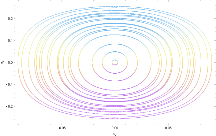
(1) $\mu_{2}=1$.

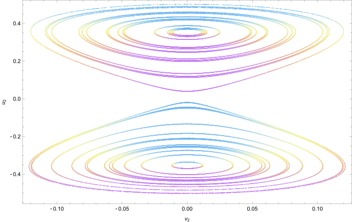
(2) $\mu_{2}=-1$.

Figure 1: Poincaré cross section $\left(v_{2},u_{2}\right)$: the integrable case $k=2$, $\mu_{1}=0.1$ and $h=0.85$.

The integrable case and some weakly perturbed cases with $k=3$, $\mu_{2}=1$ and $h=0.85$ are presented in Figure 2. For integrable case, the dynamical behavior is highly regular, see (1) of Figure 2. For sufficiently small perturbation, KAM tori appear deformation or even breaking down in the fragile top and bottom boundaries, but most of them remain for internal region, as shown in (2) and (3) of Figure 2. For $\mu_{1}=0.99$ and $\mu_{1}=0.5$, the major bifurcations occurs in the vertical direction. As the perturbation strength is increased $\mu_{1}=0.1$, the KAM tori progressively break down resulting in the trajectories complete stochastic motion. Accurately speaking, the central domain in (4) of Figure 2 is a large chaotic zone, that is, chaos. Around this chaotic zone, there are many chain of islands which correspond to quasi-periodic trajectories. Except for periodic trajectories, some KAM tori still remain in the annular area at top and bottom, which can be observed in (4) of Figure 2.

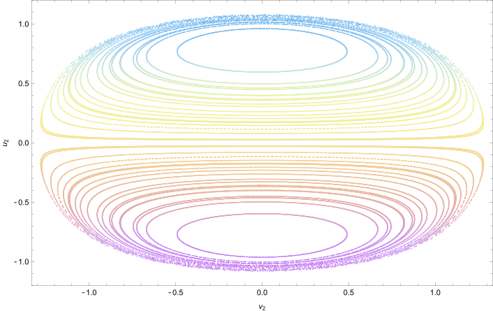
(1) $\mu_{1}=1$.

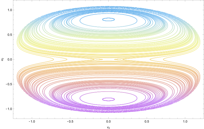
(2) $\mu_{1}=0.99$.

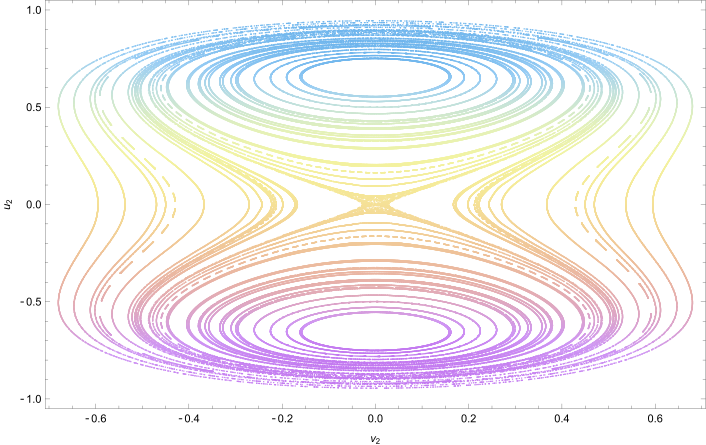
(3) $\mu_{1}=0.5$.

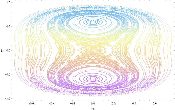
(4) $\mu_{1}=0.1$.

Figure 2: Poincaré cross section $\left(v_{2},u_{2}\right)$: $k=3$, $\mu_{2}=1$ and $h=0.85$.

Finally, our numerical simulations consider some high degree systems (1.12), that is, $k=10,20,30,40$, see Figure 3. One can see that the KAM tori at central region boundary disappear with the trajectories escaping to nonclosed areas of the phase space. This trajectories stochastic escaping create complex dynamic phenomena of system (1.12), including chaos, quasi-periodic trajectories and periodic trajectories.

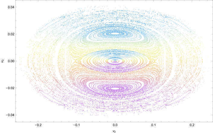
(1) $k=10$, $\mu_{2}=45$.

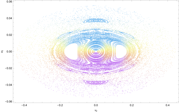
(2) $k=20$, $\mu_{2}=65$.

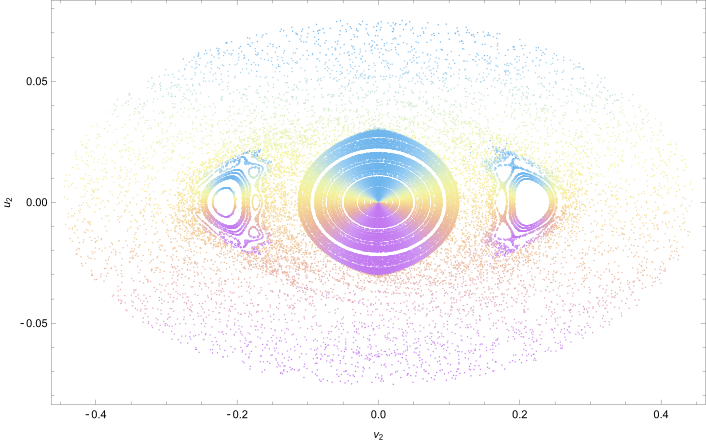
(3) $k=30$, $\mu_{2}=35$.

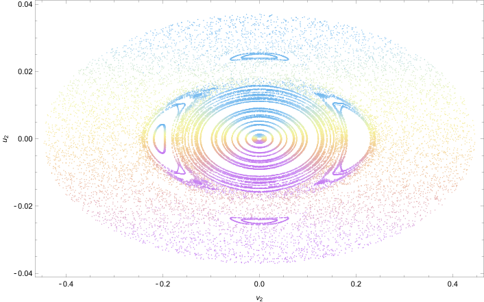
(4) $k=40$, $\mu_{2}=115$.

Figure 3: Poincaré cross section $\left(v_{2},u_{2}\right)$: for some high degree $k$ with $\mu_{1}=-1.5$ and $h=0.1$.

Appendix

Appendix A Second part of Kovacic’s algorithm

Here, we recall the second part of Kovacic’s algorithm [26]. Let $r\left(z\right)\in C\left(z\right)$ and $\Upsilon$ be the set of poles of $r\left(z\right)$. Set $\chi^{\prime\prime}=r\chi$.

• To each pole $c\in\Upsilon$, we calculate the set $\mathcal{E}_{c}$ as follows.

  • If the pole $c$ is of order $1$, then $\mathcal{E}_{c}=\left\{4\right\}$.

  • If the pole $c$ is of order $2$ and $b$ is the coefficient of $1/\left(z-c\right)^{2}$ in the partial fraction decomposition of $r\left(z\right)$, then

    $$\mathcal{E}_{c}=\left\{2+\ell\sqrt{1+4b}\;\big{|}\;\ell=0,\pm 2\right\}\bigcap\mathbb{Z}.$$ (A.1)

  • If the pole $c$ is of order $o\left(c\right)>2$, then $\mathcal{E}_{c}=\left\{o\left(c\right)\right\}$.

  • If the order of $r$ at $\infty$ is $o\left(\infty\right)>2$, then $\mathcal{E}_{c}=\left\{0,2,4\right\}$.

  • If the order of $r$ at $\infty$ is $2$ and $b$ is the coefficient of $1/z^{2}$ in the Laurent expansion of $r\left(z\right)$ at $\infty$, then

    $$\mathcal{E}_{c}=\left\{2+\ell\sqrt{1+4b}\;\big{|}\;\ell=0,\pm 2\right\}\bigcap\mathbb{Z}.$$ (A.2)

  • If the order of $r$ at $\infty$ is $o\left(\infty\right)<2$, then $\mathcal{E}_{c}=\left\{o\left(\infty\right)\right\}$.

• Let $\bm{\varpi}=\left(\varpi_{c}\right)_{c\in\Upsilon}$ be a element in the Cartesian product $\prod_{c\in\Upsilon}\mathcal{E}_{c}$ with $\varpi_{c}\in\mathcal{E}_{c}$. Define number

  $$d:=d\left(\bm{\varpi}\right)=\dfrac{1}{2}\left(\varpi_{\infty}-\sum_{c\in\Upsilon}\varpi_{c}\right).$$ (A.3)

  We try to find all elements $\bm{\varpi}$ such that $d$ is a non-negative integer, and retain such elements to perform Step 3. If there is no such element $\bm{\varpi}$, then statement (ii) of Theorem 2.4 is impossible.

• For each $\bm{\varpi}$ retained from Step 2, we introduce the rational function

  $$\theta=\dfrac{1}{2}\sum_{c\in\Upsilon}\dfrac{\varpi_{c}}{z-c}.$$

  Then, we seek a monic polynomial $P$ of degree $d$ defined in (A.3) such that

  $$P^{\prime\prime\prime}+3\theta P^{\prime\prime}+\left(3\theta^{2}+3\theta^{\prime}-4r\right)P^{\prime}+\left(\theta^{\prime\prime}+3\theta\theta^{\prime}+\theta^{3}-4r\theta-2r^{\prime}\right)P=0.$$

  If such polynomial $P$ does not exist for all elements $\bm{\varpi}$ retained from Step 2, then statement (ii) of Theorem 2.4 is untenable.

  Assume that such a polynomial $P$ exists. Let $\phi=\theta+P^{\prime}/P$ and $\omega$ be a root of

  $$\omega^{2}-\phi\omega+\left(\dfrac{1}{2}\phi^{\prime}+\dfrac{1}{2}\phi^{2}-r\right)=0.$$

  Then, $\chi=\exp\left(\int\omega\right)$ is a solution of differential equation $\chi^{\prime\prime}=r\chi$.

References

- [1] P. Acosta-Humánez, M. Alvarez-Ramírez, and T. J. Stuchi, Nonintegrability of the Armbruster-Guckenheimer-Kim quartic Hamiltonian through Morales-Ramis theory, SIAM J. Appl. Dyn. Syst., 17 (2018), 78–96.
- [2] B. Andrews and J. Clutterbuck, Proof of the fundamental gap conjecture, J. Amer. Math. Soc., 24 (2011), 899–916.
- [3] M. S. Ashbaugh and R. D. Benguria, Eigenvalue ratios for Sturm-Liouville operators, J. Differential Equations, 103 (1993), 205–219.
- [4] M. S. Ashbaugh, E. M. Harrell, II, and R. Svirsky, On minimal and maximal eigenvalue gaps and their causes, Pacific J. Math., 147 (1991), 1–24.
- [5] M. S. Ashbaugh and D. Kielty, Spectral gaps of 1-D Robin Schrödinger operators with single-well potentials, J. Math. Phys., 61 (2020), 091507, 15.
- [6] P. F. Byrd and M. D. Friedman, Handbook of elliptic integrals for engineers and physicists, Springer-Verlag, 1954.
- [7] L. M. Chasman, An isoperimetric inequality for fundamental tones of free plates, Comm. Math. Phys., 303 (2011), 421–449.
- [8] D. Chen, T. Zheng, and H. Yang, Estimates of the gaps between consecutive eigenvalues of Laplacian, Pacific J. Math., 282 (2016), 293–311.
- [9] D.-Y. Chen and M.-J. Huang, Comparison theorems for the eigenvalue gap of Schrödinger operators on the real line, Ann. Henri Poincaré, 13 (2012), 85–101.
- [10] H. Chen, M. Bhakta, and H. Hajaiej, On the bounds of the sum of eigenvalues for a Dirichlet problem involving mixed fractional Laplacians, J. Differential Equations, 317 (2022), 1–31.
- [11] H. Chen and P. Luo, Lower bounds of Dirichlet eigenvalues for some degenerate elliptic operators, Calc. Var. Partial Differential Equations, 54 (2015), 2831–2852.
- [12] Q.-M. Cheng and G. Wei, A lower bound for eigenvalues of a clamped plate problem, Calc. Var. Partial Differential Equations, 42 (2011), 579–590.
- [13] S. Y. Cheng and P. Li, Heat kernel estimates and lower bound of eigenvalues, Comment. Math. Helv., 56 (1981), 327–338.
- [14] D. V. Choodnovsky and G. V. Choodnovsky, Completely integrable class of mechanical systems connected with Korteweg-de Vries and multicomponent Schrödinger equations, Lett. Nuovo Cimento (2), 22 (1978), 47–51.
- [15] T. Combot, A. J. Maciejewski, and M. Przybylska, Bi-homogeneity and integrability of rational potentials, J. Differential Equations, 268 (2020), 7012–7028.
- [16] V. Gol’dshtein and A. Ukhlov, On the first eigenvalues of free vibrating membranes in conformal regular domains, Arch. Ration. Mech. Anal., 221 (2016), 893–915.
- [17] S. Guo, G. Meng, P. Yan, and M. Zhang, Optimal maximal gaps of Dirichlet eigenvalues of Sturm-Liouville operators, J. Math. Phys., 63 (2022), Paper No. 072701, 11.
- [18] J. Hedhly, Eigenvalue ratios for vibrating string equations with single-well densities, J. Differential Equations, 307 (2022), 476–485.
- [19] M. Horváth, On the first two eigenvalues of Sturm-Liouville operators, Proc. Amer. Math. Soc., 131 (2003), 1215–1224.
- [20] Y. Ilyasov and N. Valeev, Recovery of the nearest potential field from the observed eigenvalues, Phys. D, 426 (2021), Paper No. 132985, 6.
- [21] Y. S. Ilyasov and N. F. Valeev, On nonlinear boundary value problem corresponding to -dimensional inverse spectral problem, J. Differential Equations, 266 (2019), 4533–4543.
- [22] E. Julliard Tosel, Meromorphic parametric non-integrability; the inverse square potential, Arch. Ration. Mech. Anal., 152 (2000), 187–205.
- [23] S. Karaa, Extremal eigenvalue gaps for the Schrödinger operator with Dirichlet boundary conditions, J. Math. Phys., 39 (1998), 2325–2332.
- [24] T. Kimura, On Riemann’s equations which are solvable by quadratures, Funkcial. Ekvac., 12 (1969), 269–281.
- [25] S. Kondej and I. Veselić, Lower bounds on the lowest spectral gap of singular potential Hamiltonians, Ann. Henri Poincaré, 8 (2007), 109–134.
- [26] J. J. Kovacic, An algorithm for solving second order linear homogeneous differential equations, J. Symbolic Comput., 2 (1986), 3–43.
- [27] V. V. Kozlov, Symmetries, topology and resonances in Hamiltonian mechanics, vol. 31 of Ergebnisse der Mathematik und ihrer Grenzgebiete (3), Springer-Verlag, Berlin, 1996.
- [28] G. Kristensson, Second order differential equations, Springer, New York, 2010.
- [29] P. Kröger, Upper bounds for the Neumann eigenvalues on a bounded domain in Euclidean space, J. Funct. Anal., 106 (1992), 353–357.
- [30] P. Li and S. T. Yau, On the Schrödinger equation and the eigenvalue problem, Comm. Math. Phys., 88 (1983), 309–318.
- [31] E. H. Lieb, The number of bound states of one-body Schroedinger operators and the Weyl problem, in Geometry of the Laplace operator, Proc. Sympos. Pure Math., XXXVI, Amer. Math. Soc., Providence, R.I., 1980, 241–252.
- [32] A. J. Maciejewski, M. Przybylska, and T. Stachowiak, Non-integrability of Gross-Neveu systems, Phys. D, 201 (2005), 249–267.
- [33] A. J. Maciejewski, M. Przybylska, and A. V. Tsiganov, On algebraic construction of certain integrable and super-integrable systems, Phys. D, 240 (2011), 1426–1448.
- [34] G. Meng and M. R. Zhang, Continuity in weak topology: first order linear systems of ODE, Acta Math. Sin. (Engl. Ser.), 26 (2010), 1287–1298.
- [35] J. J. Morales Ruiz, Differential Galois theory and non-integrability of Hamiltonian systems, vol. 179 of Progress in Mathematics, Birkhäuser Verlag, Basel, 1999.
- [36] G. Pólya, On the eigenvalues of vibrating membranes, Proc. London Math. Soc. (3), 11 (1961), 419–433.
- [37] J. Pöschel and E. Trubowitz, Inverse spectral theory, vol. 130 of Pure and Applied Mathematics, Academic Press, Inc., Boston, MA, 1987.
- [38] M. Shibayama, Non-integrability of the spacial -center problem, J. Differential Equations, 265 (2018), 2461–2469.
- [39] I. M. Singer, B. Wong, S.-T. Yau, and S. S.-T. Yau, An estimate of the gap of the first two eigenvalues in the Schrödinger operator, Ann. Scuola Norm. Sup. Pisa Cl. Sci. (4), 12 (1985), 319–333.
- [40] R. S. Strichartz, Estimates for sums of eigenvalues for domains in homogeneous spaces, J. Funct. Anal., 137 (1996), 152–190.
- [41] C. J. Thompson, On the ratio of consecutive eigenvalues in -dimensions, Studies in Appl. Math., 48 (1969), 281–283.
- [42] Y. Tian, Q. Wei, and M. Zhang, On the polynomial integrability of the critical systems for optimal eigenvalue gaps, J. Math. Phys., 64 (2023), p. 092701.
- [43] N. F. Valeev and Y. S. Ilyasov, Inverse spectral problem for Sturm-Liouville operator with prescribed partial trace, Ufa Math. J., 12 (2020), 19–29.
- [44] M. van der Put and M. F. Singer, Galois theory of linear differential equations, vol. 328, Springer-Verlag, Berlin, 2003.
- [45] H. Vogt, A lower bound on the first spectral gap of Schrödinger operators with Kato class measures, Ann. Henri Poincaré, 10 (2009), 395–414.
- [46] Q. Wei, G. Meng, and M. Zhang, Extremal values of eigenvalues of Sturm-Liouville operators with potentials in balls, J. Differential Equations, 247 (2009), 364–400.
- [47] H. Weyl, Über gewöhnliche Differentialgleichungen mit Singularitäten und die zugehörigen Entwicklungen willkürlicher Funktionen, Math. Ann., 68 (1910), 220–269.
- [48] E. T. Whittaker and G. N. Watson, A course of modern analysis. An introduction to the general theory of infinite processes and of analytic functions: with an account of the principal transcendental functions, Cambridge University Press, New York, 1962.
- [49] S. Wiggins, Introduction to applied nonlinear dynamical systems and chaos, vol. 2 of Texts in Applied Mathematics, Springer-Verlag, New York, second ed., 2003.
- [50] P. Yan and M. Zhang, Continuity in weak topology and extremal problems of eigenvalues of the -Laplacian, Trans. Amer. Math. Soc., 363 (2011), 2003–2028.
- [51] P. Yan and M. Zhang, A survey on extremal problems of eigenvalues, Abstr. Appl. Anal., (2012), pp. Art. ID 670463, 26.
- [52] H. Yoshida, A criterion for the nonexistence of an additional integral in Hamiltonian systems with a homogeneous potential, Phys. D, 29 (1987), 128–142.
- [53] H. Yoshida, Nonintegrability of the truncated Toda lattice Hamiltonian at any order, Comm. Math. Phys., 116 (1988), 529–538.
- [54] M. Zhang, Continuity in weak topology: higher order linear systems of ODE, Sci. China Ser. A, 51 (2008), 1036–1058.
- [55] M. Zhang, Extremal values of smallest eigenvalues of Hill’s operators with potentials in balls, J. Differential Equations, 246 (2009), 4188–4220.