Majorana fermion induced power-law scaling in the violation of Wiedemann-Franz law

Abstract

Violation of the Wiedemann-Franz (WF) law in a 2D topological insulator due to Majorana bound states (MBS) is studied via the Lorenz ratio in the single-particle picture. We study the scaling of the Lorenz ratio in the presence and absence of MBS with inelastic scattering modeled using a Büttiker voltage-temperature probe. We compare our results with that seen in a quantum dot junction in the Luttinger liquid picture operating in the topological Kondo regime. We find that the scaling of the Lorenz ratio in our setup corresponds to the scaling in the Luttinger-liquid setup only when both phase and momentum relaxation occur, but not when only phase relaxation occurs. This suggests that the interplay between the presence of Majorana bound states and the type of inelastic scattering process, can have a significant impact on the violation of the Wiedemann-Franz law in 2D topological insulators.

I Introduction

Majorana fermions are a particular class of fermions with the unique property of being their antiparticles. Majorana fermions have intrinsic topological protection from disorder. This property renders Majorana fermions immune to decoherence, making Majorana fermions an ideal candidate for quantum computation. Various proposals to generate and detect Majorana fermions exist within the field of condensed matter physics, such as semiconductor-superconductor heterostructures [1], normal metal-superconductor heterostructures, or topological insulator-superconductor heterostructures. There have been many attempts to detect Majorana fermions experimentally [2], but there is still no irrefutable experimental evidence for the existence of Majorana fermions.

There have been proposals to detect Majorana fermions using violations in WF law [3] by studying the scaling of the Lorenz ratio. Ref. [3] studies the violation of Wiedemann-Franz law in a quantum dot junction in the topological Kondo regime [4] hosting localized Majorana bound states (MBS). WF law states that the ratio of the electrical conductance to the thermal conductance is inversely proportional to the temperature. The constant of proportionality, also known as the Lorenz ratio, is a constant for all conductors. Majorana fermions are also known to break particle-hole symmetry (PHS) and induce violations of Wiedemann-Franz (WF) law [3]. In the presence of MBS, the Lorenz ratio has been shown to scale inversely with respect to the Luttinger parameter [3]. The setup in [3] is considered in the many body regime and shows that the Lorenz ratio shows power-law decay as a function of the Luttinger parameter in the setup.

In this paper, we discuss the violation of WF law and the scaling of the Lorenz ratio in the presence of Majorana fermions using a Büttiker voltage-temperature probe [5, 6, 7], which induces inelastic scattering. We consider two kinds of inelastic scattering in our setup: first with both phase and momentum relaxation [5] while second with only phase relaxation [6]. We study the scaling of the Lorenz ratio with respect to the strength of inelastic scattering and compare the scaling of the Lorenz ratio with the Luttinger parameter in the many-body setup considered in [3]. In our setup, we study three cases: (i) when MBS are absent, (ii) when MBS are present and uncoupled, and (iii) when MBS are coupled. In a single-electron setup, the Lorenz ratio scales differently with inelastic scattering when both phase and momentum relaxation occur and when only phase relaxation occurs. For individual MBS, WF law is not violated without inelastic scattering. The rest of the paper is organized as follows: In section II, we describe the motivation and importance of this work. Section III describes the scattering and transmission in our setup using Landauer-Büttiker scattering formalism. In section IV, we first calculate the thermoelectric coefficients like the Seebeck, Peltier, and thermal conductance in our setup using the Onsager relations. We then define the Lorenz ratio and introduce inelastic scattering via a Büttiker voltage-temperature probe [7]. In section V, we present an analysis of our results and compare the scaling of the Lorenz ratio with the strength of inelastic scattering and compare it with the scaling seen in Ref. [3]. We end with the conclusions in section VI.

II Motivation

Ref [3] studies a quantum dot junction capable of hosting an even number of Majorana fermions to study the setup in the topological Kondo regime [4]. In special cases, the electrons in the quantum dot can couple to two-fold degenerate states. The regular Kondo effect [8] is a consequence of the coupling of mobile electrons in a confined region to spin-degenerate states. Further, an even number of Majorana fermions can couple non-locally, giving rise to two-fold degenerate states that can couple to electrons in the quantum dot [4]. It is known as the topological Kondo effect [4]. The setup is studied in the Luttinger liquid model, which uses many-body formalism and considers inelastic scattering due to electron-electron interaction. The electron-electron interaction is parameterized by the Luttinger parameter $(g)$, with $g=1$ corresponding to the absence of interaction, $g<1$ corresponding to attractive interaction, and $g>1$ corresponding to repulsive interaction. The authors of Ref. [3] show that the Lorenz ratio $(W)$ depends on the Luttinger parameter as $W(g)=\frac{2}{3g}$. When the setup in Ref. [3] is in the topological Kondo regime, the Majorana-induced boundary conditions and scattering via a splitting junction leads to the ”splitting” of a charged particle into a transmitted particle of charge $\frac{2e}{3}$ and a backscattered hole of charge $\frac{e}{3}$. The coefficient $\frac{2}{3}$ is the unique and universal signature of Majorana bound states in a quantum dot junction operating in the topological regime according to Ref. [3].

Our setup introduces inelastic scattering phenomenologically using Büttiker voltage probe [6, 5]. The Büttiker probe is an additional probe that induces inelastic scattering in the setup such that the total charge and heat current flowing into the Büttiker probe is zero. Unlike Luttinger liquid theory, the Büttiker voltage probe is based on single-particle scattering theory, making it more adaptable to setups studied using scattering theory. Further, using the Büttiker voltage probe, we can study inelastic scattering with phase and momentum relaxation [5] and inelastic scattering with only phase relaxation [6]. In our work, we look at both electric conductance and thermal conductance. Therefore, we modify the Büttiker voltage probe into a Büttiker voltage-temperature probe, as was also done recently in [7]. The comparison between the Luttinger parameter and inelastic scattering due to the Büttiker voltage-temperature probe [7] has not been studied before. We study the scaling of the Lorenz ratio (W) with respect to the coupling strength of the Büttiker voltage-temperature probe in our setup. A Büttiker voltage-temperature probe is added to the setup, such that the total charge and heat currents going into the probe vanish but induce inelastic scattering via both phase and momentum relaxation [5] or only phase relaxation [6]. Any electron/hole entering the Büttiker probe loses its phase memory and is reinjected with a completely different phase, leading to phase relaxation [6, 5]. For the case of both phase and momentum relaxation [5], the electrons injected into the probe from the setup are reinjected with equal probabilities of going toward the left or the right. Thus, the reinjection also causes the phase and the initial momentum to be lost. To preserve the momentum while inducing phase relaxation, one can use a pair of unidirectional probes such that when the electrons initially traveling to the left or the right are injected into the Büttiker probe, they are reinjected back with the same momentum, see Ref. [6]. We seek to probe MBS using two different kinds of Büttiker voltage-temperature probes, note the difference in these results, and compare our results with the results seen in Ref. [3], which is studied in the many body picture. This distinguishing behavior of MBS as a function of inelastic scattering in Büttiker voltage-temperature probe [7] is revealed through the Lorenz ratio. The signatures distinguish MBS’s existence and nature (coupled or individual).

III Description of the Model

III.1 Hamiltonian

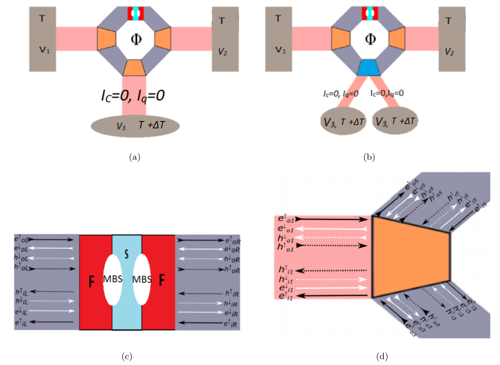
In Fig. 1, we show our proposed model. Our proposed Majorana Aharonov-Bohm interferometer (ABI) is based on helical edge modes generated via the quantum spin Hall effect in topological insulators (TIs). We mold a 2D TI into an Aharonov-Bohm ring wherein spin-orbit coupling generates protected 1D edge modes. The ring is pierced by an Aharonov-Bohm flux $\phi$. The Dirac equation for electrons and holes in the ring is given as

$$[vp\tau_{z}\sigma_{z}+(-E_{F}+\frac{eA}{\hbar c})\tau_{z}]\psi=E\psi\,.$$ (1)

$\psi=(\psi_{e\uparrow},\psi_{e\downarrow},\psi_{h\downarrow},\psi_{h\uparrow})^{T}$ is a four-component spinor, $p=-i\hbar\frac{\partial}{\partial x}$ is the momentum operator, $E_{F}$ is the Fermi energy, $E$ is the incident electron energy, $v_{F}$ is the Fermi velocity, and $A$ is the magnetic vector potential. MBS (shown in white) occurs in the upper half of the ring at the junction between the superconducting and ferromagnetic layer in the TI (STIM junction) (see Fig. 1) [9, 10, 11]. The Hamiltonian for the MBS is [12, 11],

$$H_{M}=-\sigma_{y}E_{M}\,,$$ (2)

with $E_{M}$ denoting coupling strength between individual MBS. The STIM junction is connected to the left and right arms of the ring with coupling strengths $\Gamma_{1}$ and $\Gamma_{2}$, respectively. In the next subsection, we outline the scattering via edge modes in the setup and calculate the transmission probability $\mathcal{T}$.

Figure 1: (a) The 3 terminal Majorana Aharonov-Bohm interferometer with a Büttiker voltage temperature probe, with both phase and momentum relaxation [5]. A 2D TI ring with helical edge modes flowing in the outer and inner edges. The ring is coupled to two regular TI leads via couplers (shown in orange). The leads connect the AB ring to the reservoirs. A third coupler connects the ring to an inelastic scatterer acting as a Büttiker voltage-temperature probe [7], such that the total charge and heat current flowing in the third terminal is zero. The ring is pierced by an Aharonov-Bohm flux. Ferromagnetic (shown in red) and superconducting (shown in cyan) correlations are induced in the top arm of the ring via the proximity effect. (b) The Majorana Aharonov-Bohm interferometer with a Büttiker voltage-temperature probe with only phase relaxation [6], the Büttiker voltage-temperature probe consists of two unidirectional probes attached to the bottom via a coupler such that the total charge and heat currents into each probe terminal is zero. The electrons injected into each probe terminal are reinjected back into the setup via the other probe, preserving the momentum. (c) The superconductor-topological insulator-ferromagnet (STIM) junction. MBS (shown as white ellipses) occurs at the interface of the ferromagnetic (shown in red) and superconducting (shown in cyan) layer. (d) Scattering of the edge modes at the left coupler. The solid and dashed lines represent the electron and hole edge modes. The black and white lines represent the spin-up and spin-down edge modes. The double-headed arrows represent the outer edge modes, and the single-headed arrows represent the inner edge modes, respectively.

III.2 Transport in the system via edge modes

In a 2D quantum Hall ring with an Aharonov-Bohm flux, localized flux-sensitive edge modes develop near the hole, while in the leads (shown in pink in Fig. 1), edge modes are insensitive to flux. To tune the device via an Aharonov-Bohm flux, we need to couple the edge modes in the leads and the edge modes in the ring so that the net conductance is flux-sensitive. It can be achieved via couplers (shown in orange in Fig. 1) in the system that couples the inner and outer edge modes via inter-edge scattering and backscattering. There are three leads in the setup coupled to the ring. The left and right couplers are connected to reservoirs at voltage $V_{1}$ on the left, $V$ on the right, and temperatures $T$ at the left and right reservoirs. A pair of MBS occur in the STIM junction on the top of the ring and act as a backscatter, mixing the electron and hole edge modes. Considering the electron and hole edge modes of spins up and down, we get $8$ edge modes with $4$ edge modes circulating on the outer edge and $4$ edge modes circulating on the inner edge. Since spin-flip scattering does not occur in our setup, we can significantly simplify the calculation by dividing the edge modes into two sets of edge modes of opposite spin that scatter as mirror images. It allows us to calculate the transmission probabilities for a single set and double it to get the net conductance.
The first set consists of the spin-up electron and spin-up hole edge modes, and the second set consists of counterpropagating spin-down electron and spin-down hole edge modes. The STIM junction couples the incoming and outgoing edge modes of each set. Among the spin-up edge modes, incoming edge modes into the STIM junction are given by $I_{MBS1}=(e^{\uparrow}_{oL},e^{\uparrow}_{iR},h^{\uparrow}_{oL},h^{\uparrow}_{iR})$ and the outgoing edge modes are given by $O_{MBS1}=(e^{\uparrow}_{oR},e^{\uparrow}_{iL},h^{\uparrow}_{oR},h^{\uparrow}_{iL})$ (see Fig. 1 (b)). Similarly, among the spin-down edge modes, the incoming edge modes are $I_{MBS2}=(e^{\downarrow}_{oR},e^{\downarrow}_{iL},h^{\downarrow}_{oR},h^{\downarrow}_{iL})$, while the outgoing edge modes are $O_{MBS2}=(e^{\downarrow}_{oL},e^{\downarrow}_{iR},h^{\downarrow}_{oL},h^{\downarrow}_{iR})$. The scattering in each case is the exact mirror image of the other. We can relate the incoming and outgoing edge modes using a $4\times 4$ scattering matrix $S_{MBS}$ such that $O_{MBSi}=S_{MBS}I_{MBSi},i\in\{1,2\}$, where $S_{MBS}$ is given by [11, 12]

$$S_{MBS}=\begin{pmatrix}1+ix&-y&ix&-y\\ y&1+ix^{\prime}&y&ix^{\prime}\\ ix&-y&1+ix&-y\\ y&ix^{\prime}&y&1+ix^{\prime}\end{pmatrix}$$ (3a)

where,

$$\begin{split}x=\frac{\Gamma_{1}(E+i\Gamma_{2})}{z},x^{\prime}=\frac{\Gamma_{2}(E+i\Gamma_{1})}{z},\\ y=\frac{E_{M}\sqrt{\Gamma_{1}\Gamma_{2}}}{z},z=E_{M}^{2}-(E+i\Gamma_{1})(E+i\Gamma_{2})\,\end{split}$$ (3b)

and $\Gamma_{1}$, $\Gamma_{2}$ are the strengths of the couplers coupling the MBS to the left and right arms of the upper ring.
The couplers (see Fig. 1 (d)) couple the inner and outer edge modes via backscattering and the ring to the leads. In the left coupler, the incoming spin-up edge modes are given by $I_{1}=(e^{\uparrow}_{o1},h^{\uparrow}_{o1},e^{\uparrow}_{o3},h^{\uparrow}_{o3},e^{\uparrow}_{i5},h^{\uparrow}_{i5})$, and the corresponding spin-up outgoing edge modes are given by $O_{1}=(e^{\uparrow}_{i1},h^{\uparrow}_{i1},e^{\uparrow}_{i3},h^{\uparrow}_{i3},e^{\uparrow}_{o5},h^{\uparrow}_{o5})$. Similarly, the incoming spin-down edge modes are given by $I_{2}=(e^{\uparrow}_{i2},h^{\uparrow}_{i2},e^{\uparrow}_{i4},h^{\uparrow}_{i4},e^{\uparrow}_{o6},h^{\uparrow}_{o6})$, and the corresponding outgoing spin-down edge modes are $O_{2}=(e^{\uparrow}_{o2},h^{\uparrow}_{o2},e^{\uparrow}_{o4},h^{\uparrow}_{o4},e^{\uparrow}_{i6},h^{\uparrow}_{i6})$. The scattering matrix for the couplers is a $6\times 6$ matrix $S$ such that $O_{i}=SI_{i},i\in\{1,2\}$ is given by [5]

$$S=\begin{pmatrix}-\frac{1}{3}I&&\frac{2}{3}I&&\frac{2}{3}I\\ &&&&\\ \frac{2}{3}I&&-\frac{1}{3}I&&\frac{2}{3}I\\ &&&\\ \frac{2}{3}I&&\frac{2}{3}I&&-\frac{1}{3}I\end{pmatrix},$$ (4)

where $I$ is the $2\times 2$ identity matrix. This S-matrix is obtained by taking $\epsilon=\frac{4}{9}$ in Büttiker’s $3\times 3$ S-matrix, see Ref. [5]. The reason for using this S-matrix is that it corresponds exactly to a waveguide result, see Ref. [13]. While traversing the ring, the spin-up electrons and holes in the edge modes acquire a propagating phase [12] as follows:
in the upper arm, left of the STIM junction:

$$\begin{split}e^{\uparrow}_{i5}=e^{ik_{e}l_{1}}e^{\frac{-i\phi l_{1}}{L}}e^{\uparrow}_{iL},e^{\uparrow}_{oL}=e^{ik_{e}l_{1}}e^{\frac{i\phi l_{1}}{L}}e^{\uparrow}_{o5},\\ h^{\uparrow}_{i5}=e^{ik_{h}l_{1}}e^{\frac{i\phi l_{1}}{L}}h^{\uparrow}_{iL},h^{\uparrow}_{oL}=e^{ik_{h}l_{1}}e^{\frac{-i\phi l_{1}}{L}}h^{\uparrow}_{o5},\end{split}$$ (5)

for the upper arm, right of STIM junction:

$$\begin{split}e^{\uparrow}_{o6}=e^{ik_{e}l_{2}}e^{\frac{i\phi l_{2}}{L}}e^{\uparrow}_{oR},e^{\uparrow}_{iR}=e^{ik_{e}l_{2}}e^{\frac{-i\phi l_{2}}{L}}e^{\uparrow}_{i6},\\ h^{\uparrow}_{o6}=e^{ik_{h}l_{2}}e^{\frac{-i\phi l_{2}}{L}}h^{\uparrow}_{oR},h^{\uparrow}_{iR}=e^{ik_{h}l_{2}}e^{\frac{i\phi l_{2}}{L}}h^{\uparrow}_{i6},\end{split}$$ (6)

such that $l_{1}+l_{2}=l_{u}$, i.e. length of the upper arm of the ring. For the lower arm of the ring, left of the Büttiker voltage-temperature probe:

$$\begin{split}e^{\uparrow}_{o3}=e^{ik_{e}l^{\prime}_{1}}e^{\frac{i\phi l^{\prime}_{2}}{L}}e^{\uparrow}_{o4},e^{\uparrow}_{i4}=e^{ik_{d}l^{\prime}_{1}}e^{\frac{-i\phi l^{\prime}_{2}}{L}}e^{\uparrow}_{i3},\\ h^{\uparrow}_{o3}=e^{ik_{h}l^{\prime}_{1}}e^{\frac{-i\phi l^{\prime}_{2}}{L}}h^{\uparrow}_{o4},h^{\uparrow}_{i4}=e^{ik_{h}l^{\prime}_{1}}e^{\frac{i\phi l^{\prime}_{2}}{L}}h^{\uparrow}_{i3},\end{split}$$ (7)

for the lower arm of the ring, right of the Büttiker voltage-temperature probe:

$$\begin{split}e^{\uparrow}_{o4}=e^{ik_{e}l^{\prime}_{1}}e^{\frac{i\phi l^{\prime}_{2}}{L}}e^{\uparrow}_{o5},e^{\uparrow}_{i5}=e^{ik_{d}l^{\prime}_{1}}e^{\frac{-i\phi l^{\prime}_{2}}{L}}e^{\uparrow}_{i4},\\ h^{\uparrow}_{o4}=e^{ik_{h}l^{\prime}_{1}}e^{\frac{-i\phi l^{\prime}_{2}}{L}}h^{\uparrow}_{o5},h^{\uparrow}_{i5}=e^{ik_{h}l^{\prime}_{1}}e^{\frac{i\phi l^{\prime}_{2}}{L}}h^{\uparrow}_{i4},\end{split}$$ (8)

such that $l^{\prime}_{1}+l^{\prime}_{2}=l_{d}$, i.e., the length of the bottom arm of the ring. The total length of the ring $L$ is given by $L=l_{u}+l_{d}$. $k_{e}=(E+E_{f})/\hbar v_{F}$, and $k_{h}=(E-E_{f})/\hbar v_{F}$ are electron and hole wave vectors in the 2D TI. $\phi$ is the Aharonov-Bohm flux taken in units of the flux quantum $\phi_{0}=hc/e$. One can similarly find the phase acquired by the spin-down electrons and holes, which is the exact mirror image of spin-up electrons and holes. In the next section, we describe thermoelectric transport in multi-terminal mesoscopic systems and introduce inelastic scattering by adding a Büttiker voltage-temperature probe [5, 6, 7] to the Majorana ABI.

IV Inelastic scattering and Büttiker voltage-temperature probe

We explain the thermoelectric transport in our setup shown in Fig. 1 using Onsager relations [14] and Landauer-Büttiker scattering theory [15]. We denote the charge and heat currents in the $i^{th}$ terminal by current vector $I^{s}_{i}=(I^{s}_{ic},I^{s}_{iq}),$ where $I^{s}_{ic}=I^{s,e}_{ic}+I^{s,h}_{ic}$ is the total charge current, and $I^{s}_{iq}=I^{s,e}_{iq}+I^{s,h}_{iq}$ the total heat current with spin $s\in\{\uparrow,\downarrow\}$ electrons and holes. The current vector $I^{sk}_{i}=(I^{sk}_{ic},I^{sk}_{iq})^{T}$ can be related to force vector $F_{ij}=(V_{j},\Delta T_{ij})^{T}$ (where $V_{j}$ is the voltage at the $j^{th}$ terminal, and $\Delta T_{ij}=T_{j}-T_{i}$ is the temperature difference across the $i^{th}$ and the $j^{th}$ terminals) by the Onsager matrix $L^{sr;kl}_{ij}$ such that $I^{sk}_{i}=\sum_{j,r,l}L^{sr;kl}_{ij}F_{ij}$, where [14, 16],

where $\delta_{ij}$ is the Dirac Delta function, $f(E,E_{F})$ being the Fermi function $(f(E,E_{F})=\frac{1}{1+e^{(E-E_{F})/k_{B}T_{i}}}$), with $\xi(E,E_{F})=\frac{-\partial f(E,E_{F})}{\partial E}$, $T$ is the temperature of the left and right reservoirs. In contrast, $T+\Delta T$ is the temperature of the Büttiker voltage-temperature probe, $k_{B}$ is the Boltzmann constant, $G_{0}=(e^{2}/\hbar)$ is the conductance quantum, $E$ is particle energy, $E_{F}$ is Fermi energy, and $h$ is Planck’s constant. The Onsager matrix elements describe the thermal and electrical response to the voltage and temperature bias. $L^{sr;kl}_{ij;cV}$, is the electrical conductance, $L^{sr;kl}_{ij;cT}$ is the electrical response to the temperature difference, $L^{sr;kl}_{ij;qV}$ is the thermal response to the voltage difference, and $L^{sr;kl}_{ij;qT}$ is the thermal response generated due to the temperature difference due to a spin $r$ electron or hole ($l\in\{e,h\}$) being transmitted from the $j^{th}$ terminal into the $i^{th}$ terminal as a spin $s$ electron or hole ($k\in\{e,h\}$). $\mathcal{T}^{sr;kl}_{ij}$ is the transmission probability for an electron or hole ($l=e,h$) with spin $r$ incident from the $j^{th}$ terminal to transmit as an electron or hole ($k=e,h$) with spin $s$ in the $i^{th}$ terminal. MBS is a superposition of electrons and holes of the same spin; thus, the scattering due to MBS can cause electron-electron or electron-hole scattering between particles of the same spin. Since the opposite spin edge modes are mirror images of each other and there is no spin-flip scattering in our system (see Fig. 1), we can write $\mathcal{T}^{\uparrow\uparrow}_{ij;kl}=\mathcal{T}^{\downarrow\downarrow}_{ij;kl}$, and $\mathcal{T}^{\uparrow\downarrow}_{ij;kl}=\mathcal{T}^{\uparrow\downarrow}_{ij;kl}=0$. From Eq. (9), we can write [17]:

$$\begin{split}\small I^{\uparrow e}_{ic}=\sum_{j}L^{\uparrow\uparrow;ee}_{ij;cV}V_{j}+\sum_{j}L^{\uparrow\uparrow;ee}_{ij;cT}\Delta T_{ij},\\ \text{ and }I^{\uparrow e}_{iq}=\sum_{j}L^{\uparrow\uparrow;ee}_{ij;qV}V_{j}+\sum_{j}L^{\uparrow\uparrow;ee}_{ij;qT}\Delta T_{ij},\\ \end{split}$$ (11a)

$$\begin{split}\small I^{\downarrow e}_{ic}=\sum_{j}L^{\downarrow\downarrow;ee}_{ij;cV}V_{j}+\sum_{j}L^{\downarrow\downarrow;ee}_{ij;cT}\Delta T_{ij},\\ \text{ and }I^{\downarrow e}_{iq}=\sum_{j}L^{\downarrow\downarrow;ee}_{ij;qV}V_{j}+\sum_{j}L^{\downarrow\downarrow;ee}_{ij;qT}\Delta T_{ij},\\ \end{split}$$ (11b)

$$\begin{split}\small I^{\uparrow h}_{ic}=\sum_{j}L^{\uparrow\uparrow;he}_{ij;cV}V_{j}+\sum_{j}L^{\uparrow\uparrow;he}_{ij;cT}\Delta T_{ij},\\ \text{ and }I^{\uparrow h}_{iq}=\sum_{j}L^{\uparrow\uparrow;he}_{ij;qV}V_{j}+\sum_{j}L^{\uparrow\uparrow;he}_{ij;qT}\Delta T_{ij},\\ \end{split}$$ (11c)

$$\begin{split}\small I^{\downarrow h}_{ic}=\sum_{j}L^{\downarrow\downarrow;he}_{ij;cV}V_{j}+\sum_{j}L^{\downarrow\downarrow;he}_{ij;cT}\Delta T_{ij},\\ \text{ and }I^{\downarrow h}_{iq}=\sum_{j}L^{\downarrow\downarrow;he}_{ij;qV}V_{j}+\sum_{j}L^{\downarrow\downarrow;he}_{ij;qT}\Delta T_{ij}.\\ \end{split}$$ (11d)

This section will introduce inelastic scattering in our system using a Büttiker voltage-temperature probe [7]. In the setup shown in Fig. 1, an additional lead is connected to the ABI via a coupler that connects the ABI to a Büttiker voltage-temperature probe such that the total charge current and the total heat current flowing into terminal 3 are zero. The S-matrices for the left and right couplers are described in Eq. (4), and they scatter electrons/holes elastically. The voltage-temperature probe induces inelastic scattering by setting the total charge and heat current passing through itself to zero. It ensures that no net current flows out of the setup into the probe (in section IV, analysis, we will look at the scaling of the Lorenz ratio with respect to the strength of inelastic scattering in the single-particle picture). We study two types of inelastic scattering in our setup, with only phase relaxation [6] and with both phase relaxation and momentum relaxation [5]. We compare and contrast our result with that obtained using Luttinger formalism [3].

IV.1 Inelastic scattering with both phase and momentum relaxation

In the first model (see Fig. 1 (a)), we use an inelastic scatterer with both phase and momentum relaxation [5]. The S-matrix for this first inelastic scattering model with both phase and momentum relaxation, henceforth referred to as $B3$ is given by [5],

$$S=\begin{pmatrix}-(p+q)I&\sqrt{\epsilon}I&\sqrt{\epsilon}I\\ \sqrt{\epsilon}I&pI&qI\\ \sqrt{\epsilon}I&qI&pI\end{pmatrix},$$ (12)

the matrix for the STIM junction is given by Eq. (3a). We also look at a symmetric three-way coupler that can induce inelastic scattering with phase and momentum relaxation, henceforth referred to as $S3$. The S-matrix for the symmetric three-way scatterer [18] is given by,

$$S=\begin{pmatrix}r&tI&tI\\ tI&rI&tI\\ rI&rI&tI\end{pmatrix},$$ (13)

where $r=-2\cos(\epsilon)e^{i\epsilon}/\sqrt{1+8\cos^{2}(\epsilon)}$ is the reflection amplitude and $t=1/\sqrt{1+8\cos^{2}(\epsilon)}$ is the transmission amplitude.
Using Landauer-Büttiker scattering theory, we can find the charge and heat currents in each terminal of the setup described in Fig. 1 (a). In our work, the left and right terminals are at voltages $V_{1}=0$, and $V_{2}=V$, respectively; both terminals are at temperature $T$. The Büttiker voltage-temperature probe is at temperature $T+\Delta T$, and voltage $V_{3}$. From Eq. (11), we can write the charge and heat currents for our setup in terms of the Onsager elements as,

We are solving Eqs. (3-8) and using Eqs. (12, 13) for the S-matrix of the Büttiker voltage-temperature probe, one can find the transmission probabilities $\mathcal{T}^{sr;kl}_{ij}$ in the setup. Plugging the transmission probabilities in Eqs. (14-17), along with Eq. (9), allows us to calculate the charge and heat currents in each terminal. We represent the charge and heat currents in terms of the voltage and temperature biases in a matrix notation below: The charge currents in each terminal due to spin-up electrons and holes are given by,

$$\begin{pmatrix}I^{\uparrow e}_{1c}\\ I^{\uparrow h}_{1c}\\ I^{\uparrow e}_{2c}\\ I^{\uparrow h}_{2c}\\ I^{\uparrow e}_{3c}\\ I^{\uparrow h}_{3c}\\ \end{pmatrix}=-\begin{pmatrix}G(\mathcal{T}^{\uparrow\uparrow;ee}_{12})&G(\mathcal{T}^{\uparrow\uparrow;ee}_{13})&S(\mathcal{T}^{\uparrow\uparrow;ee}_{13})\\ G(\mathcal{T}^{\uparrow\uparrow;he}_{12})&G(\mathcal{T}^{\uparrow\uparrow;he}_{13})&S(\mathcal{T}^{\uparrow\uparrow;he}_{13})\\ -G(1-\mathcal{T}^{\uparrow\uparrow;ee}_{22})&G(\mathcal{T}^{\uparrow\uparrow;ee}_{23})&S(\mathcal{T}^{\uparrow\uparrow;ee}_{23})\\ -G(1-\mathcal{T}^{\uparrow\uparrow;he}_{22})&G(\mathcal{T}^{\uparrow\uparrow;he}_{23})&S(\mathcal{T}^{\uparrow\uparrow;he}_{23})\\ G(\mathcal{T}^{\uparrow\uparrow;ee}_{32})&-G(1-\mathcal{T}^{\uparrow\uparrow;ee}_{33})&-S(\mathcal{T}^{\uparrow\uparrow;ee}_{31})-S(\mathcal{T}^{\uparrow\uparrow;ee}_{32})\\ G(\mathcal{T}^{\uparrow\uparrow;he}_{32})&-G(1-\mathcal{T}^{\uparrow\uparrow;he}_{33})&-S(\mathcal{T}^{\uparrow\uparrow;he}_{31})-S(\mathcal{T}^{\uparrow\uparrow;he}_{32})\\ \end{pmatrix}\begin{pmatrix}V\\ V_{3}\\ \Delta T\end{pmatrix},$$ (18)

The corresponding heat currents due to spin-up electrons and holes are given by:

$$\begin{pmatrix}I_{1q}^{\uparrow e}\\ I_{1q}^{\uparrow h}\\ I_{2q}^{\uparrow e}\\ I_{2q}^{\uparrow h}\\ I_{3q}^{\uparrow e}\\ I_{3q}^{\uparrow h}\\ \end{pmatrix}=-\begin{pmatrix}S(\mathcal{T}^{\uparrow\uparrow;ee}_{12})&S(\mathcal{T}^{\uparrow\uparrow;ee}_{13})&L(\mathcal{T}^{\uparrow\uparrow;ee}_{13})\\ S(\mathcal{T}^{\uparrow\uparrow;he}_{12})&S(\mathcal{T}^{\uparrow\uparrow;he}_{13})&L(\mathcal{T}^{\uparrow\uparrow;he}_{13})\\ -S(1-\mathcal{T}^{\uparrow\uparrow;ee}_{22})&S(\mathcal{T}^{\uparrow\uparrow;ee}_{23})&L(\mathcal{T}^{\uparrow\uparrow;ee}_{23})\\ -S(1-\mathcal{T}^{\uparrow\uparrow;he}_{22})&S(\mathcal{T}^{\uparrow\uparrow;he}_{23})&L(\mathcal{T}^{\uparrow\uparrow;he}_{23})\\ S(\mathcal{T}^{\uparrow\uparrow;ee}_{32})&-S(1-\mathcal{T}^{\uparrow\uparrow;ee}_{33})&-L(\mathcal{T}^{\uparrow\uparrow;ee}_{31})-L(\mathcal{T}^{\uparrow\uparrow;ee}_{32})\\ S(\mathcal{T}^{\uparrow\uparrow;he}_{32})&S(1-\mathcal{T}^{\uparrow\uparrow;he}_{33})&-L(\mathcal{T}^{\uparrow\uparrow;he}_{31})+-L(\mathcal{T}^{\uparrow\uparrow;he}_{32})\\ \end{pmatrix}\begin{pmatrix}V\\ V_{3}\\ \Delta T\end{pmatrix},$$ (19)

Similarly, for the spin-down electrons and holes, the charge currents are given as,

$$\begin{pmatrix}I^{\downarrow e}_{1c}\\ I^{\downarrow h}_{1c}\\ I^{\downarrow e}_{2c}\\ I^{\downarrow h}_{2c}\\ I^{\downarrow e}_{3c}\\ I^{\downarrow h}_{3c}\\ \end{pmatrix}=-\begin{pmatrix}G(\mathcal{T}^{\downarrow\downarrow;ee}_{12})&G(\mathcal{T}^{\downarrow\downarrow;ee}_{13})&S(\mathcal{T}^{\downarrow\downarrow;ee}_{13})\\ G(\mathcal{T}^{\downarrow\downarrow;he}_{12})&G(\mathcal{T}^{\downarrow\downarrow;he}_{13})&S(\mathcal{T}^{\downarrow\downarrow;he}_{13})\\ -G(1-\mathcal{T}^{\downarrow\downarrow;ee}_{22})&G(\mathcal{T}^{\downarrow\downarrow;ee}_{23})&S(\mathcal{T}^{\downarrow\downarrow;ee}_{23})\\ -G(1-\mathcal{T}^{\downarrow\downarrow;he}_{22})&G(\mathcal{T}^{\downarrow\downarrow;he}_{23})&S(\mathcal{T}^{\downarrow\downarrow;he}_{23})\\ G(\mathcal{T}^{\downarrow\downarrow;ee}_{32})&-G(1-\mathcal{T}^{\downarrow\downarrow;ee}_{33})&-S(\mathcal{T}^{\downarrow\downarrow;ee}_{31})-S(\mathcal{T}^{\downarrow\downarrow;ee}_{32})\\ G(\mathcal{T}^{\downarrow\downarrow;he}_{32})&-G(1-\mathcal{T}^{\downarrow\downarrow;he}_{33})&-S(\mathcal{T}^{\downarrow\downarrow;he}_{31})-S(\mathcal{T}^{\downarrow\downarrow;he}_{32})\\ \end{pmatrix}\begin{pmatrix}V\\ V_{3}\\ \Delta T\end{pmatrix},$$ (20)

and the corresponding heat currents due to spin-down electrons and holes are given by:

$$\begin{pmatrix}I_{1q}^{\downarrow e}\\ I_{1q}^{\downarrow h}\\ I_{2q}^{\downarrow e}\\ I_{2q}^{\downarrow h}\\ I_{3q}^{\downarrow e}\\ I_{3q}^{\downarrow h}\\ \end{pmatrix}=-\begin{pmatrix}S(\mathcal{T}^{\downarrow\downarrow;ee}_{12})&S(\mathcal{T}^{\downarrow\downarrow;ee}_{13})&L(\mathcal{T}^{\downarrow\downarrow;ee}_{13})\\ S(\mathcal{T}^{\downarrow\downarrow;he}_{12})&S(\mathcal{T}^{\downarrow\downarrow;he}_{13})&L(\mathcal{T}^{\downarrow\downarrow;he}_{13})\\ -S(1-\mathcal{T}^{\downarrow\downarrow;ee}_{22})&S(\mathcal{T}^{\downarrow\downarrow;ee}_{23})&L(\mathcal{T}^{\downarrow\downarrow;ee}_{23})\\ -S(1-\mathcal{T}^{\downarrow\downarrow;he}_{22})&S(\mathcal{T}^{\downarrow\downarrow;he}_{23})&L(\mathcal{T}^{\downarrow\downarrow;he}_{23})\\ S(\mathcal{T}^{\downarrow\downarrow;ee}_{32})&-S(1-\mathcal{T}^{\downarrow\downarrow;ee}_{33})&-L(\mathcal{T}^{\downarrow\downarrow;ee}_{31})-L(\mathcal{T}^{\downarrow\downarrow;ee}_{32})\\ S(\mathcal{T}^{\downarrow\downarrow;he}_{32})&-S(1-\mathcal{T}^{\downarrow\downarrow;he}_{33})&-L(\mathcal{T}^{\downarrow\downarrow;he}_{31})-L(\mathcal{T}^{\downarrow\downarrow;he}_{32})\\ \end{pmatrix}\begin{pmatrix}V\\ V_{3}\\ \Delta T\end{pmatrix},$$ (21)

where $G(X)$ is the electrical conductance for particles with transmission probability $X$, $S(X)$ is the Seebeck coefficient for particles with transmission probability $X$, and $L(X)$ is the thermal conductance for particles with transmission probability $X$. We can calculate the charge and heat currents for both the Büttiker S-matrix given in Eq. (12) and the symmetric three-way scatterer given in Eq. (13) by using the respective S-matrix for the Büttiker voltage-temperature probe [7] when solving for the transmission probabilities $\mathcal{T}^{sr;kl}_{ij}$. In Eqs. (18-21) the electrical conductance $G(\mathcal{T}^{sr;kl}_{ij}(E))$ for a particle with transmission probability $\mathcal{T}^{sr;kl}_{ij}(E)$ is given by,

$$G(\mathcal{T}^{sr;kl}_{ij}(E))=G_{0}\int_{-\infty}^{\infty}dE\mathcal{T}^{sr;kl}_{ij}(E)(-\frac{df}{dE}),$$ (22)

the Seebeck coefficient $S(\mathcal{T}^{sr;kl}_{ij}(E))$ for a particle with transmission probability $\mathcal{T}^{sr;kl}_{ij}(E)$ is given by,

$$S(\mathcal{T}^{sr;kl}_{ij}(E))=G_{0}\int_{-\infty}^{\infty}dE(E-\mu)\mathcal{T}^{sr;kl}_{ij}(E)(-\frac{df}{dE}).$$ (23)

The Peltier coefficient is the opposite of the Seebeck coefficient and is given by $P(\mathcal{T}^{sr;kl}_{ij}(E))=-S(\mathcal{T}^{sr;kl}_{ij}(E))$. The thermal conductance $L(\mathcal{T}^{sr;kl}_{ij}(E))$ for a particle with transmission probability $\mathcal{T}^{sr;kl}_{ij}(E)$ is given by,

$$L(\mathcal{T}^{sr;kl}_{ij}(E))=G_{0}\int_{-\infty}^{\infty}dE(E-\mu)^{2}\mathcal{T}^{sr;kl}_{ij}(E)(-\frac{df}{dE}).$$ (24)

The total charge current in the Büttiker voltage-temperature probe is thus given by,

$$I_{3c}=I^{\uparrow e}_{3c}+I^{\uparrow h}_{3c}+I^{\downarrow e}_{3c}+I^{\downarrow h}_{3c},$$ (25)

and the total heat current is given by,

$$I_{3q}=I^{\uparrow e}_{3q}+I^{\uparrow h}_{3q}+I^{\downarrow e}_{3q}+I^{\downarrow h}_{3q}.$$ (26)

In order to introduce inelastic scattering via the Büttiker voltage-temperature probe, we should have $I_{3c}(V,T+\Delta T)=I_{3q}(V,T+\Delta T)=0$. In our setup, we measure the charge and heat currents in the second terminal. The total charge current in the second terminal is given by,

$$I_{2c}=I^{\uparrow e}_{2c}+I^{\uparrow h}_{2c}+I^{\downarrow e}_{2c}+I^{\downarrow h}_{2c},$$ (27)

and the total heat current is given by,

$$I_{2q}=I^{\uparrow e}_{2q}+I^{\uparrow h}_{2q}+I^{\downarrow e}_{2q}+I^{\downarrow h}_{2q}.$$ (28)

In order to find the thermoelectric coefficients and, subsequently, the Lorenz ratio, we write $I_{2q}$ and $I_{2c}$ in terms of $V$ and $\Delta T$ only by eliminating $V_{3}$ from Eqs. (18-21). We use the condition of the Büttiker voltage-temperature probe ($I_{3c}(V,T+\Delta T)=I_{3q}(V,T+\Delta T)=0$) in order to write all the voltages and temperatures in terms of $V$ and $\Delta T$. Thus, $I_{2c}$ and $I_{2q}$ can now be written solely in terms of $V$ and $\Delta T$ as,

$$\small I_{2c}=L^{\prime}_{cV}V+L^{\prime}_{cT}\Delta T\text{ and }I_{2q}=L^{\prime}_{qV}V+L^{\prime}_{qT}\Delta T,$$ (29)

where $L^{\prime}_{cV},L^{\prime}_{qV},L^{\prime}_{cT},L^{\prime}_{qT}$ are the effective Onsager coefficients for conduction in the second terminal and are functions of $G(\mathcal{T}^{sr;kl}_{ij}(E))$, $S(\mathcal{T}^{sr;kl}_{ij}(E))$, $L(\mathcal{T}^{sr;kl}_{ij}(E))$ as defined in Eqs. (22-24). $L^{\prime}_{cV}$ is the effective electrical conductance in the second terminal given as, $L^{\prime}_{cV}=\frac{I_{2c}}{V}|_{\Delta T=0}.$ $L^{\prime}_{cT}$ is the electrical response to the temperature difference and is given by $L^{\prime}_{cT}=\frac{I_{2c}}{\Delta T}|_{V=0}$. Similarly, the thermal response to the voltage difference $L^{\prime}_{qV}$ is given by $L^{\prime}_{qV}=\frac{I_{2q}}{V}|_{\Delta T=0}$, and the thermal response to the temperature difference is given by $L^{\prime}_{qT}=\frac{I_{2q}}{\Delta T}|_{V=0}$. The effective Onsager coefficients are then given as,

$$L^{\prime}_{cV}=\sum_{s}\Bigg{[}G(1-\mathcal{T}^{ss;ee}_{22})+G(1-\mathcal{T}^{ss;he}_{22})-\delta[(G(\mathcal{T}^{ss;ee}_{31})+G(\mathcal{T}^{ss;he}_{31}))(G(\mathcal{T}^{ss;ee}_{32})+G(\mathcal{T}^{ss;he}_{32}))]\Bigg{]}$$ (30)

$$L^{\prime}_{cT}=\sum_{s}\Bigg{[}-S(\mathcal{T}^{ss;ee}_{22})-S(\mathcal{T}^{ss;he}_{22})-\delta[(S(1-\mathcal{T}^{ss;ee}_{31})+S(1-\mathcal{T}^{ss;he}_{31}))(S(1-\mathcal{T}^{ss;ee}_{32})+S(1-\mathcal{T}^{ss;he}_{32}))]\Bigg{]}$$ (31)

$$L^{\prime}_{qV}=\sum_{s}\Bigg{[}-S(1-\mathcal{T}^{ss;ee}_{22})-S(1-\mathcal{T}^{ss;he}_{22})-\delta[(S(\mathcal{T}^{ss;ee}_{31})+S(\mathcal{T}^{ss;he}_{31}))(S(\mathcal{T}^{ss;ee}_{32})+S(\mathcal{T}^{ss;he}_{32}))]\Bigg{]}$$ (32)

$$L^{\prime}_{qT}=\sum_{s}\Bigg{[}-L(\mathcal{T}^{ss;ee}_{22})-L(\mathcal{T}^{ss;he}_{22})+\delta[(L(1-\mathcal{T}^{ss;ee}_{31})+L(1-\mathcal{T}^{ss;he}_{31}))(S(1-\mathcal{T}^{ss;ee}_{32})+S(1-\mathcal{T}^{ss;he}_{32}))]\Bigg{]},$$ (33)

where $\delta=\dfrac{1}{G(1-\mathcal{T}^{ss;ee}_{33})+G(1-\mathcal{T}^{ss;he}_{33})}$. The effective electrical conductance is the total charge current generated due to the voltage difference and is given by $\sigma^{\prime}=L^{\prime}_{cV}$. The effective thermal conductance [19] is the heat current generated by a unit temperature bias without any charge current. The effective thermal conductance of the setup with $3\times 3$ Büttiker probe with both phase and momentum relaxation is then given by,

$$\kappa^{\prime}=\frac{I_{2q}}{\Delta T}|_{I_{ic}=0}=\frac{L^{\prime}_{cV}L^{\prime}_{qT}-L^{\prime}_{cT}L^{\prime}_{qV}}{L^{\prime}_{cV}}.$$ (34)

Wiedemann–Franz (WF) law states that the ratio of the effective thermal conductance ($\kappa^{\prime}$) to the effective electric conductance ($\sigma^{\prime}$) is proportional to the temperature [20] of the TI ($T$). We define the Lorenz ratio $W$ as,

$$W=\frac{\kappa^{\prime}}{\sigma^{\prime}}.$$ (35)

When WF law is preserved, $W=W_{0}$, where $W_{0}=\frac{\kappa_{0}}{G_{0}}$, where $G_{0}=\dfrac{e^{2}}{\hbar}$ and $\kappa_{0}=\pi^{2}k_{B}^{2}T/3h$, where $T$ is temperature of the reservoirs 1 and 2. WF law is derived from the fact that in condensed matter systems, both charge and heat are carried by the quasiparticles in the conductor, namely, the electrons and holes. Quasiparticles in conductors generally follow particle-hole symmetry (PHS), i.e., the electron energy levels are symmetric to the hole energy levels. When PHS is preserved in the system, WF law is preserved, and the Lorenz ratio is not violated [20, 21]. The breakdown of PHS causes violations of WF law. In the next subsection, we include inelastic scattering with the help of the Büttiker voltage-temperature probe but with phase relaxation only.

IV.2 Inelastic scattering with only phase relaxation

Fig. 1 (b) shows the MBS ABI with only phase relaxation [6]. The third terminal, i.e., the Büttiker voltage-temperature probe, is divided into two terminals that are connected to reservoirs at voltage $V_{3}$ and temperature $T+\Delta T$ such that the total charge current and heat current flowing in each terminal is zero. The inelastic scatterers are connected via a coupler described by a $4\times 4$ scattering matrix given by [6],

$$S_{p}=\begin{pmatrix}0&\sqrt{1-\epsilon}I&0&-\sqrt{\epsilon}I\\ \sqrt{1-\epsilon}I&0&-\sqrt{\epsilon}I&0\\ \sqrt{\epsilon}I&0&\sqrt{1-\epsilon}I&0\\ 0&\sqrt{\epsilon}I&0&\sqrt{1-\epsilon}I\end{pmatrix},$$ (36)

where $\epsilon\in[0,1]$, and $I$ is the $2\times 2$ scattering matrix. $\epsilon=1$ denotes maximal coupling, while $\epsilon\to 0$ denotes no coupling [6]. Similar to the setup in Fig. 1 (a), we can relate the charge and heat currents to the voltage and temperature difference using Landauer-Büttiker scattering theory. We set the voltage of the left terminal at zero and the temperature at $T$, while the right terminal is at voltage $V$ and temperature $T$. Using Eq. (11), we relate the charge and heat currents to the voltage and temperature biases in matrix form as,

Finding the transmission probabilities $\mathcal{T}^{sr;kl}_{ij}$ from Eqs. (3-8) and using Eq. (36) for the S-matrix of the inelastic scatterer, we can find the charge current in each terminal of the setup in Fig. 1 (b), i.e., with only phase relaxation as,

$$\begin{pmatrix}I_{1c}^{\uparrow e}\\ I_{1c}^{\uparrow h}\\ I_{2c}^{\uparrow e}\\ I_{2c}^{\uparrow h}\\ I_{3c}^{\uparrow e}\\ I_{3c}^{\uparrow h}\\ I_{4c}^{\uparrow e}\\ I_{4c}^{\uparrow h}\end{pmatrix}=-\begin{pmatrix}G(\mathcal{T}^{\uparrow\uparrow;ee}_{12})&G(\mathcal{T}^{\uparrow\uparrow;ee}_{13})&G(\mathcal{T}^{\uparrow\uparrow;ee}_{14})&S(\mathcal{T}^{\uparrow\uparrow;ee}_{13})&S(\mathcal{T}^{\uparrow\uparrow;ee}_{14})\\ G(\mathcal{T}^{\uparrow\uparrow;he}_{12})&G(\mathcal{T}^{\uparrow\uparrow;he}_{13})&G(\mathcal{T}^{\uparrow\uparrow;he}_{14})&S(\mathcal{T}^{\uparrow\uparrow;he}_{13})&S(\mathcal{T}^{\uparrow\uparrow;he}_{14})\\ -G(1-\mathcal{T}^{\uparrow\uparrow;ee}_{22})&G(\mathcal{T}^{\uparrow\uparrow;ee}_{23})&G(\mathcal{T}^{\uparrow\uparrow;ee}_{24})&S(\mathcal{T}^{\uparrow\uparrow;ee}_{23})&S(\mathcal{T}^{\uparrow\uparrow;ee}_{24})\\ -G(1-\mathcal{T}^{\uparrow\uparrow;he}_{22})&G(\mathcal{T}^{\uparrow\uparrow;he}_{23})&G(\mathcal{T}^{\uparrow\uparrow;he}_{24})&S(\mathcal{T}^{\uparrow\uparrow;he}_{23})&S(\mathcal{T}^{\uparrow\uparrow;he}_{24})\\ G(\mathcal{T}^{\uparrow\uparrow;ee}_{32})&-G(1-\mathcal{T}^{\uparrow\uparrow;ee}_{33})&G(\mathcal{T}^{\uparrow\uparrow;ee}_{34})&-S(\mathcal{T}^{\uparrow\uparrow;ee}_{31})&-S(\mathcal{T}^{\uparrow\uparrow;ee}_{32})\\ G(\mathcal{T}^{\uparrow\uparrow;he}_{32})&-G(1-\mathcal{T}^{\uparrow\uparrow;he}_{33})&G(\mathcal{T}^{\uparrow\uparrow;he}_{34})&-S(\mathcal{T}^{\uparrow\uparrow;he}_{31})&-S(\mathcal{T}^{\uparrow\uparrow;he}_{31})\\ G(\mathcal{T}^{\uparrow\uparrow;ee}_{42})&G(\mathcal{T}^{\uparrow\uparrow;ee}_{43})&-G(1-\mathcal{T}^{\uparrow\uparrow;ee}_{44})&-S(\mathcal{T}^{\uparrow\uparrow;ee}_{41})&S(\mathcal{T}^{\uparrow\uparrow;ee}_{42})\\ G(\mathcal{T}^{\uparrow\uparrow;he}_{42})&G(\mathcal{T}^{\uparrow\uparrow;he}_{43})&-G(1-\mathcal{T}^{\uparrow\uparrow;he}_{44})&-S(\mathcal{T}^{\uparrow\uparrow;he}_{41})&S(\mathcal{T}^{\uparrow\uparrow;he}_{42})\end{pmatrix}\begin{pmatrix}V\\ V_{3}\\ V_{3}\\ \Delta T\\ \Delta T\end{pmatrix},$$ (41)

The corresponding heat currents due to spin-up electrons and holes are,

$$\begin{pmatrix}I_{1c}^{\uparrow e}\\ I_{1c}^{\uparrow h}\\ I_{2c}^{\uparrow e}\\ I_{2c}^{\uparrow h}\\ I_{3c}^{\uparrow e}\\ I_{3c}^{\uparrow h}\\ I_{4c}^{\uparrow e}\\ I_{4c}^{\uparrow h}\end{pmatrix}=-\begin{pmatrix}S(\mathcal{T}^{\uparrow\uparrow;ee}_{12})&S(\mathcal{T}^{\uparrow\uparrow;ee}_{13})&S(\mathcal{T}^{\uparrow\uparrow;ee}_{14})&L(\mathcal{T}^{\uparrow\uparrow;ee}_{13})&L(\mathcal{T}^{\uparrow\uparrow;ee}_{14})\\ S(\mathcal{T}^{\uparrow\uparrow;he}_{12})&S(\mathcal{T}^{\uparrow\uparrow;he}_{13})&S(\mathcal{T}^{\uparrow\uparrow;he}_{14})&L(\mathcal{T}^{\uparrow\uparrow;he}_{13})&L(\mathcal{T}^{\uparrow\uparrow;he}_{14})\\ -S(1-\mathcal{T}^{\uparrow\uparrow;ee}_{22})&S(\mathcal{T}^{\uparrow\uparrow;ee}_{23})&S(\mathcal{T}^{\uparrow\uparrow;ee}_{24})&L(\mathcal{T}^{\uparrow\uparrow;ee}_{23})&L(\mathcal{T}^{\uparrow\uparrow;ee}_{24})\\ -S(1-\mathcal{T}^{\uparrow\uparrow;he}_{22})&S(\mathcal{T}^{\uparrow\uparrow;he}_{23})&S(\mathcal{T}^{\uparrow\uparrow;he}_{24})&L(\mathcal{T}^{\uparrow\uparrow;he}_{23})&L(\mathcal{T}^{\uparrow\uparrow;he}_{24})\\ S(\mathcal{T}^{\uparrow\uparrow;ee}_{32})&-S(1-\mathcal{T}^{\uparrow\uparrow;ee}_{33})&S(\mathcal{T}^{\uparrow\uparrow;ee}_{34})&-L(\mathcal{T}^{\uparrow\uparrow;ee}_{31})&-L(\mathcal{T}^{\uparrow\uparrow;ee}_{32})\\ S(\mathcal{T}^{\uparrow\uparrow;he}_{32})&-S(1-\mathcal{T}^{\uparrow\uparrow;he}_{33})&S(\mathcal{T}^{\uparrow\uparrow;he}_{34})&-L(\mathcal{T}^{\uparrow\uparrow;he}_{31})&-L(\mathcal{T}^{\uparrow\uparrow;he}_{32})\\ S(\mathcal{T}^{\uparrow\uparrow;ee}_{42})&S(\mathcal{T}^{\uparrow\uparrow;ee}_{43})&-S(1-\mathcal{T}^{\uparrow\uparrow;ee}_{44})&-L(\mathcal{T}^{\uparrow\uparrow;ee}_{41})&L(\mathcal{T}^{\uparrow\uparrow;ee}_{42})\\ S(\mathcal{T}^{\uparrow\uparrow;he}_{42})&S(\mathcal{T}^{\uparrow\uparrow;he}_{43})&-S(1-\mathcal{T}^{\uparrow\uparrow;he}_{44})&-L(\mathcal{T}^{\uparrow\uparrow;he}_{41})&L(\mathcal{T}^{\uparrow\uparrow;he}_{42})\end{pmatrix}\begin{pmatrix}V\\ V_{3}\\ V_{3}\\ \Delta T\\ \Delta T\end{pmatrix},$$ (42)

Similarly, the total current due to spin-down electrons and holes is given by,

$$\begin{pmatrix}I_{1c}^{\downarrow e}\\ I_{1c}^{\downarrow h}\\ I_{2c}^{\downarrow e}\\ I_{2c}^{\downarrow h}\\ I_{3c}^{\downarrow e}\\ I_{3c}^{\downarrow h}\\ I_{4c}^{\downarrow e}\\ I_{4c}^{\downarrow h}\end{pmatrix}=-\begin{pmatrix}G(\mathcal{T}^{\downarrow\downarrow;ee}_{12})&G(\mathcal{T}^{\downarrow\downarrow;ee}_{13})&G(\mathcal{T}^{\downarrow\downarrow;ee}_{14})&S(\mathcal{T}^{\downarrow\downarrow;ee}_{13})&S(\mathcal{T}^{\downarrow\downarrow;ee}_{14})\\ G(\mathcal{T}^{\downarrow\downarrow;he}_{12})&G(\mathcal{T}^{\downarrow\downarrow;he}_{13})&G(\mathcal{T}^{\downarrow\downarrow;he}_{14})&S(\mathcal{T}^{\downarrow\downarrow;he}_{13})&S(\mathcal{T}^{\downarrow\downarrow;he}_{14})\\ -G(1-\mathcal{T}^{\downarrow\downarrow;ee}_{22})&G(\mathcal{T}^{\downarrow\downarrow;ee}_{23})&G(\mathcal{T}^{\downarrow\downarrow;ee}_{24})&S(\mathcal{T}^{\downarrow\downarrow;ee}_{23})&S(\mathcal{T}^{\downarrow\downarrow;ee}_{24})\\ -G(1-\mathcal{T}^{\downarrow\downarrow;he}_{22})&G(\mathcal{T}^{\downarrow\downarrow;he}_{23})&G(\mathcal{T}^{\downarrow\downarrow;he}_{24})&S(\mathcal{T}^{\downarrow\downarrow;he}_{23})&S(\mathcal{T}^{\downarrow\downarrow;he}_{24})\\ G(\mathcal{T}^{\downarrow\downarrow;ee}_{32})&-G(1-\mathcal{T}^{\downarrow\downarrow;ee}_{33})&G(\mathcal{T}^{\downarrow\downarrow;ee}_{34})&-S(\mathcal{T}^{\downarrow\downarrow;ee}_{31})&-S(\mathcal{T}^{\downarrow\downarrow;ee}_{32})\\ G(\mathcal{T}^{\downarrow\downarrow;he}_{32})&-G(1-\mathcal{T}^{\downarrow\downarrow;he}_{33})&G(\mathcal{T}^{\downarrow\downarrow;he}_{34})&-S(\mathcal{T}^{\downarrow\downarrow;he}_{31})&-S(\mathcal{T}^{\downarrow\downarrow;he}_{32})\\ G(\mathcal{T}^{\downarrow\downarrow;ee}_{42})&G(\mathcal{T}^{\downarrow\downarrow;ee}_{43})&-G(1-\mathcal{T}^{\downarrow\downarrow;ee}_{44})&-S(\mathcal{T}^{\downarrow\downarrow;ee}_{41})&S(\mathcal{T}^{\downarrow\downarrow;ee}_{42})\\ G(\mathcal{T}^{\downarrow\downarrow;he}_{42})&G(\mathcal{T}^{\downarrow\downarrow;he}_{43})&-G(1-\mathcal{T}^{\downarrow\downarrow;he}_{44})&-S(\mathcal{T}^{\downarrow\downarrow;he}_{41})&S(\mathcal{T}^{\downarrow\downarrow;he}_{42})\end{pmatrix}\begin{pmatrix}V\\ V_{3}\\ V_{3}\\ \Delta T\\ \Delta T\end{pmatrix},$$ (43)

and the corresponding heat currents due to spin-down electrons and holes, as,

$$\begin{pmatrix}I_{1c}^{\downarrow e}\\ I_{1c}^{\downarrow h}\\ I_{2c}^{\downarrow e}\\ I_{2c}^{\downarrow h}\\ I_{3c}^{\downarrow e}\\ I_{3c}^{\downarrow h}\\ I_{4c}^{\downarrow e}\\ I_{4c}^{\downarrow h}\end{pmatrix}=-\begin{pmatrix}S(\mathcal{T}^{\downarrow\downarrow;ee}_{12})&S(\mathcal{T}^{\downarrow\downarrow;ee}_{13})&S(\mathcal{T}^{\downarrow\downarrow;ee}_{14})&L(\mathcal{T}^{\downarrow\downarrow;ee}_{13})&L(\mathcal{T}^{\downarrow\downarrow;ee}_{14})\\ S(\mathcal{T}^{\downarrow\downarrow;he}_{12})&S(\mathcal{T}^{\downarrow\downarrow;he}_{13})&S(\mathcal{T}^{\downarrow\downarrow;he}_{14})&L(\mathcal{T}^{\downarrow\downarrow;he}_{13})&L(\mathcal{T}^{\downarrow\downarrow;he}_{14})\\ -S(1-\mathcal{T}^{\downarrow\downarrow;ee}_{22})&S(\mathcal{T}^{\downarrow\downarrow;ee}_{23})&S(\mathcal{T}^{\downarrow\downarrow;ee}_{24})&L(\mathcal{T}^{\downarrow\downarrow;ee}_{23})&L(\mathcal{T}^{\downarrow\downarrow;ee}_{24})\\ -S(1-\mathcal{T}^{\downarrow\downarrow;he}_{22})&S(\mathcal{T}^{\downarrow\downarrow;he}_{23})&S(\mathcal{T}^{\downarrow\downarrow;he}_{24})&L(\mathcal{T}^{\downarrow\downarrow;he}_{23})&L(\mathcal{T}^{\downarrow\downarrow;he}_{24})\\ S(\mathcal{T}^{\downarrow\downarrow;ee}_{32})&-S(1-\mathcal{T}^{\downarrow\downarrow;ee}_{33})&S(\mathcal{T}^{\downarrow\downarrow;ee}_{34})&-L(\mathcal{T}^{\downarrow\downarrow;ee}_{31})&-L(\mathcal{T}^{\downarrow\downarrow;ee}_{32})\\ S(\mathcal{T}^{\downarrow\downarrow;he}_{32})&-S(1-\mathcal{T}^{\downarrow\downarrow;he}_{33})&S(\mathcal{T}^{\downarrow\downarrow;he}_{34})&-L(\mathcal{T}^{\downarrow\downarrow;he}_{31})&-L(\mathcal{T}^{\downarrow\downarrow;he}_{32})\\ S(\mathcal{T}^{\downarrow\downarrow;ee}_{42})&S(\mathcal{T}^{\downarrow\downarrow;ee}_{43})&-S(1-\mathcal{T}^{\downarrow\downarrow;ee}_{44})&-L(\mathcal{T}^{\downarrow\downarrow;ee}_{41})&L(\mathcal{T}^{\downarrow\downarrow;ee}_{42})\\ S(\mathcal{T}^{\downarrow\downarrow;he}_{42})&S(\mathcal{T}^{\downarrow\downarrow;he}_{43})&-S(1-\mathcal{T}^{\downarrow\downarrow;he}_{44})&-L(\mathcal{T}^{\downarrow\downarrow;he}_{41})&L(\mathcal{T}^{\downarrow\downarrow;he}_{42})\end{pmatrix}\begin{pmatrix}V\\ V_{3}\\ V_{3}\\ \Delta T\\ \Delta T\end{pmatrix},$$ (44)

where $G(X)$ is the electrical conductance for particles with transmission probability $X$, $S(X)$ is the Seebeck coefficient for particles with transmission probability $X$, and $L(X)$ is the thermal conductance for particles with transmission probability $X$. The electrical, Seebeck, and thermal conductances are given in Eqs. (22-24). Similar to the derivation of the Onsager matrix elements for the inelastic scatterer with both phase and momentum relaxation, one can find the Onsager matrix elements for the inelastic scatterer with only phase relaxation. First, we write Eqs. (41-44) in terms of $V$, and $\Delta T$ only by using the condition of the Büttiker voltage-temperature probe ($I_{3c}(V,T+\Delta T)=I_{3q}(V,T+\Delta T)=I_{4c}(V,T+\Delta T)=I_{4q}(V,T+\Delta T)=0$). This allows us to write $I_{2c}$, and $I_{2q}$ in terms of $V$ and $\Delta T$ only as,

$$\begin{split}\small I_{2c}=L^{\prime\prime}_{cV}V+L^{\prime\prime}_{cT}\Delta T\text{, and }I_{2q}=L^{\prime\prime}_{qV}V+L^{\prime\prime}_{qT}\Delta T.\\ \end{split}$$ (45)

In Eq. (45) $L^{\prime\prime}_{cV},L^{\prime\prime}_{cT},L^{\prime\prime}_{qV},L^{\prime\prime}_{qT}$ are the effective Onsager matrix elements for the setup with phase relaxation only (see Fig. 1 (b)) and are given by,

where $\Delta=G(\mathcal{T}^{ss;ee}_{34})+G(\mathcal{T}^{ss;ee}_{43})-G(1-\mathcal{T}^{ss;ee}_{33})-G(1-\mathcal{T}^{ss;ee}_{44})+G(\mathcal{T}^{ss;he}_{34})+G(\mathcal{T}^{ss;he}_{43})-G(1-\mathcal{T}^{ss;he}_{33})-G(1-\mathcal{T}^{ss;he}_{44})$. The effective Onsager matrix elements can find all the thermoelectric coefficients. For the setup with the Büttiker voltage-temperature probe with phase relaxation only, the thermal conductance is given by [22, 23],

$$\kappa^{\prime\prime}=\frac{I_{2q}}{\Delta T}|_{I_{ic}=0}=\frac{L^{\prime\prime}_{cV}L^{\prime\prime}_{qT}-L^{\prime\prime}_{cT}L^{\prime\prime}_{qV}}{L^{\prime\prime}_{cV}}.$$ (50)

The Lorenz ratio for the setup with the Büttiker voltage-temperature probe with phase relaxation only is then given by,

$$W=\dfrac{\kappa^{{}^{\prime\prime}}}{\sigma^{\prime\prime}},\text{where, }\sigma^{\prime\prime}=L^{\prime\prime}_{cV}$$ (51)

The Mathematica codes are available in GitHub [24].

Figure 2: The Lorenz ratio ($W$) vs. the coupling strength of the inelastic scatterer $\epsilon$ for (a) the Büttiker scatterer (Eq. (12)) [5], and (b) the symmetric three-way scatterer with both phase and momentum relaxation (Eq. (13)) [18]. (c) Büttiker scatterer with only phase relaxation (Eq. (36)) [6].

Setup		Coupled MBS	Individual MBS
Topological Kondo Model [3]		N/A	$W=\dfrac{0.66}{g}$
MBS-ABI with both phase and momentum relaxation	(i) Büttiker $3\times 3$ S-matrix [5]	$W=\dfrac{1.71}{\epsilon}$	$W=\dfrac{0.84}{\epsilon}$
	(ii) Symmetric three-way scatterer [18]	$W=\dfrac{1.61}{\epsilon}$	$W=\dfrac{0.78}{\epsilon}$
MBS-ABI with phase relaxation only [6]		$W=\dfrac{0.6}{\epsilon^{3/2}}$	$W=\dfrac{0.4}{\epsilon^{3/2}}$

Table 1: Comparing the violation of WF law in our setup with the topological Kondo model [3]. The authors of Ref. [3] only study individual MBS. We study both individual and coupled MBS. In all cases, we see power law dependence of the Lorenz ratio on inelastic scattering; the power law factors are different for inelastic scattering with both phase and momentum relaxation and with only phase relaxation.

V Analysis: Violation of WF law phenomenologically vs. Luttinger liquid model

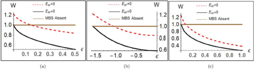
In Fig. 2, we plot the Lorenz ratio vs. the strength of inelastic scattering for the setup with both phase and momentum relaxation [5, 18], and the setup with only phase relaxation [6] in the presence of coupled MBS, individual MBS, and the absence of MBS. We use the parameters, Fermi energy $E_{F}=10\mu eV$, and flux $\phi=\phi_{0}$, $\phi_{0}$ being the flux quantum $hc/e$. In the absence of MBS, WF law is preserved in all three cases, i.e., $W=1$ for the $3\times 3$ Buttiker scatterer with both phase and momentum relaxation (Fig. 2 (a)), henceforth referred to as $B3$, the three-way symmetric scatterer with both phase and momentum relaxation (Fig. 2 (b)), henceforth referred to as $S3$, as well as the $4\times 4$ Buttiker scatterer with only phase relaxation (Fig. 2 (c)), henceforth referred to as $B4$ regardless of inelastic scattering parameter $\epsilon$.

In the presence of MBS, we consider two cases: individual MBS and coupled MBS. In our setups, we consider the MBS $E_{M}couplingstrength=10\mu eV$. The violation in Wiedemann-Franz law is most prominent when $E_{F}$ is close to $E_{M}$. Thus, to distinguish between individual MBS ($E_{M}=0$), and coupled MBS ($E_{M}=10\mu eV$), we take $E_{F}=10\mu eV$.

For $B3$[5], and $B4$[6], for $\epsilon\to 0$, the Büttiker voltage-temperature probe is completely disconnected, and there is no inelastic scattering in the setup. For $S3$, [18], the voltage-temperature probe is completely disconnected for $\epsilon\to-\pi/2$. When MBS are uncoupled or individual ($E_{M}=0$), the Lorenz ratio ($W$) is one at the limit of no inelastic scattering and decays with increasing strength of inelastic scattering ($\epsilon$). For the Luttinger liquid setup with individual MBS studied in Ref. [3], the Lorenz ratio $W$ passes through one at $g=1$, i.e., in the absence of inelastic scattering. In our setup, the Lorenz ratio $W$ is one in the absence of inelastic scattering for individual MBS. Thus, our results for individual MBS corroborate the findings of the Luttinger liquid model studied in Ref. [3]. For $B3$[5], the Lorenz ratio scales with inelastic scattering ($\epsilon$) as $W=\frac{0.84}{\epsilon}$. For $S3$[18], the Lorenz ratio scales with $\epsilon$ as $W=\frac{0.78}{\epsilon}$. Finally, for $B4$[6], the Lorenz ratio scales with $\epsilon$ as $W=\frac{0.4}{\epsilon^{3/2}}$. Thus, the Lorenz ratio $W$ is inversely proportional to the strength of inelastic scattering $\epsilon$ for inelastic scattering with both phase and momentum relaxation ($S3$ and $B3$). The Lorenz ratio scales inversely with $\epsilon^{3/2}$ for inelastic scattering with phase relaxation only ($B4$).

For coupled MBS, $E_{M}=10\mu eV\neq 0$, we see that the Lorenz ratio is greater than one in the absence of inelastic scattering for all three cases, i.e., $W>1$ for $\epsilon\to 0$ for $B3$[5], $\epsilon\to-\pi/2$ for $S3$[18], and $\epsilon\to 0$ for $B4$. In the presence of coupled MBS, PHS is broken such that the majority of electrons and holes travel in the same direction. It leads to a reduction in the net charge current and a commensurate increase in the heat current. Thus, in the presence of coupled MBS, WF law is violated even in the limit of zero inelastic scattering. The Lorenz ratio decays with increasing $\epsilon$ universally in the presence of MBS, regardless of whether they are coupled or uncoupled. For $B3$[5], the Lorenz ratio passes through one at $\epsilon=0.13$ (see Fig. 2 (a)). For $S3$[18], the Lorenz ratio passes through one at $\epsilon=-1.08$ (see Fig. 2 (b)). While for $B4$, the Lorenz ratio passes through one at $\epsilon=0.08$ (see Fig. 2 (c)). Thus, in the presence of coupled MBS, inelastic scattering can recover the WF law at a particular $\epsilon$. From Fig. 2, we find that the Lorenz ratio $W$ scaling with respect to inelastic scattering $\epsilon$ also follows the power-law for coupled MBS. For $B3$[5](Fig. 2 (a)), the Lorenz ratio scales with inelastic scattering ($\epsilon$) as $W=\frac{1.71}{\epsilon}$. For $S3$[18], the Lorenz ratio scales with $\epsilon$ as $W=\frac{1.61}{\epsilon}$. For $B4$[6], the Lorenz ratio scales with $\epsilon$ as $W=\frac{0.6}{\epsilon^{3/2}}$. Thus, the Lorenz ratio for coupled MBS is inversely proportional to $\epsilon$ when both phase and momentum relaxation are present ($S3$ and $B3$). In the presence of inelastic scattering with phase relaxation only, the Lorenz ratio is inversely proportional to $\epsilon^{3/2}$ ($B4$).

We compare our results with the Luttinger liquid model studied in Ref. [3] in Table I. The setup in Ref. [3] considers a quantum dot junction hosting MBS in the topological Kondo regime using the many-body formalism. The Luttinger parameter $g$ describes electron-electron interaction in the many-body picture with $g=1$ corresponding to no interaction. The authors in Ref. [3] report that weakly coupled MBS ($E_{M}\approx 0$) violate WF law. The authors show that the Lorenz ratio scales as $W=\frac{2}{3g}$, i.e., the Lorenz ratio is inversely proportional to the Luttinger parameter in the presence of uncoupled MBS. In our setup, the strength of inelastic scattering $\epsilon$ is analogous to the Luttinger parameter $g$ used in Ref. [3]. When both phase and momentum relaxation are present in the setup, the Lorenz ratio is inversely proportional to $\epsilon$. Thus, Table I shows that the setup with both phase and momentum relaxation is much closer to the model described in Ref. [3]. According to our results, the electron-electron interaction described by the Luttinger parameter $g$ results in inelastic scattering with both phase and momentum relaxation.

From Table I, we can see that the scaling of the Lorenz ratio changes when both phase and momentum relaxation are present in the setup and when only phase relaxation is present in the setup. In our setup, the major violations in WF law arise due to the breaking of PHS by the MBS in the upper arm. In the upper arm, MBS causes electron-hole mixing and backscattering [11]. For both phase and momentum relaxation, the electrons and holes in the lower arm are transmitted, and backscattered [25]. This backscattering can counteract the breaking of PHS by MBS and lead to a weaker violation. Similar effects have been observed in Ref. [26] wherein the authors observe the restoration of WF law due to inelastic scattering. When only phase relaxation is present, the electrons and holes continue to travel in the same direction they initially traveled. Thus, they do not strongly counteract the breaking of PHS by the MBS. It can explain why the scatterer affects the violations more strongly with only phase relaxation. Thus, we see that the scaling changes in the presence of only phase relaxation. The unique scaling of the Lorenz ratio in the presence of MBS with only phase relaxation and with both phase and momentum relaxation can be used as a signature for MBS.

VI Conclusion

We studied the violation of Wiedemann-Franz law in both the presence as well as absence of MBS via the scaling of the Lorenz ratio as a function of the strength of inelastic scattering. Inelastic scattering is induced by a Büttiker voltage-temperature probe. We find that WF law is only violated in the presence of MBS. We studied the scaling of the Lorenz ratio in the presence of inelastic scattering with both phase and momentum relaxation and with only phase relaxation and compared our results with those of the Luttinger liquid model studied in Ref. [3]. We showed that the Lorenz ratio decays with increasing strength of inelastic scattering when MBS are present, irrespective of whether they are individual or coupled. The Luttinger liquid model predicts that the Lorenz ratio is inversely proportional to the Luttinger parameter with $W(g)=\frac{2}{3g}$. In the presence of individual MBS, for the $3\times 3$ Buttiker S-matrix [5] with both phase and momentum relaxation, the Lorenz ratio scales with inelastic scattering ($\epsilon$) as $W=\frac{0.84}{\epsilon}$. For the symmetric three-way scatterer [18] with both phase and momentum relaxation, the Lorenz ratio scales with $\epsilon$ as $W=\frac{0.78}{\epsilon}$. For $4\times 4$ Buttiker S-matrix with phase relaxation only [6], the Lorenz ratio scales with $\epsilon$ as $W=\frac{0.4}{\epsilon^{3/2}}$. When MBS in the setup are coupled, the scaling is similar with $W=\frac{1.71}{\epsilon}$ for the $3\times 3$ Buttiker S-matrix [5]. $W=\frac{1.61}{\epsilon}$ for the symmetric three-way scatterer [18], and $W=\frac{0.6}{\epsilon^{3/2}}$ for $4\times 4$ Buttiker S-matrix with phase relaxation only [6]. The results show that the electron-electron interaction in the Luttinger liquid model is similar to the inelastic scattering induced phenomenologically by the Büttiker voltage-temperature probe [7] with both phase and momentum relaxation [5, 18]. Further, we show that for coupled MBS, the Lorenz ratio is greater than one when inelastic scattering is absent and decays with increasing $\epsilon$. For individual MBS, the Lorenz ratio is conserved without inelastic scattering and decays when inelastic scattering is introduced. This distinct behavior of the Lorenz ratio in the scaling can be used to detect MBS.

References

• Lutchyn et al. [2018] R. M. Lutchyn, E. P. A. M. Bakkers, L. P. Kouwenhoven, P. Krogstrup, C. M. Marcus, and Y. Oreg, Nature Reviews Materials 3, 52 (2018).
• Zhang et al. [2021] H. Zhang, C.-X. Liu, S. Gazibegovic, D. Xu, J. A. Logan, G. Wang, N. van Loo, J. D. S. Bommer, M. W. A. de Moor, D. Car, R. L. M. Op het Veld, P. J. van Veldhoven, S. Koelling, M. A. Verheijen, M. Pendharkar, D. J. Pennachio, B. Shojaei, J. S. Lee, C. J. Palmstrøm, E. P. A. M. Bakkers, S. Das Sarma, and L. P. Kouwenhoven, Nature 591, E30 (2021).
• Buccheri et al. [2022] F. Buccheri, A. Nava, R. Egger, P. Sodano, and D. Giuliano, Phys. Rev. B 105, L081403 (2022).
• Béri and Cooper [2012] B. Béri and N. R. Cooper, Phys. Rev. Lett. 109, 156803 (2012).
• Büttiker [1985] M. Büttiker, Physical Review B 32, 1846 (1985).
• Büttiker [1986] M. Büttiker, Phys. Rev. B 33, 3020 (1986).
• Kilgour and Segal [2016] M. Kilgour and D. Segal, The Journal of Chemical Physics 144, 124107 (2016).
• Hewson [1997] A. C. Hewson, The Kondo problem to heavy fermions, Cambridge university press  (1997).
• Fu and Kane [2008] L. Fu and C. L. Kane, Phys. Rev. Lett. 100, 096407 (2008).
• Fu and Kane [2009] L. Fu and C. L. Kane, Phys. Rev. B 79, 161408 (2009).
• Nilsson et al. [2008] J. Nilsson, A. R. Akhmerov, and C. W. J. Beenakker, Phys. Rev. Lett. 101, 120403 (2008).
• Benjamin and Pachos [2010] C. Benjamin and J. K. Pachos, Phys. Rev. B 81, 085101 (2010).
• Benjamin [2016] C. Benjamin, “Electron transport and quantum interference at the mesoscopic scale”, Ph. D Thesis, Institute of Physics, Bhubaneswar, India (2004), LAP Lambert Academic Publishing  (2016).
• Hofer and Sothmann [2015] P. P. Hofer and B. Sothmann, Phys. Rev. B 91, 195406 (2015).
• Buttiker et al. [1983] M. Buttiker, Y. Imry, and R. Landauer, Physics Letters A 96, 365 (1983).
• Samuelsson et al. [2017] P. Samuelsson, S. Kheradsoud, and B. Sothmann, Phys. Rev. Lett. 118, 256801 (2017).
• Benenti et al. [2011] G. Benenti, K. Saito, and G. Casati, Phys. Rev. Lett. 106, 230602 (2011).
• Heikkilä [2013] T. T. Heikkilä, The physics of nanoelectronics: transport and fluctuation phenomena at low temperatures, Oxford University Press  (2013).
• Mani and Benjamin [2019] A. Mani and C. Benjamin, The Journal of Physical Chemistry C 123, 22858 (2019).
• Franz and Wiedemann [1853] R. Franz and G. Wiedemann, Annalen der Physik 165, 497 (1853).
• Ramos-Andrade et al. [2016] J. P. Ramos-Andrade, O. Ávalos-Ovando, P. A. Orellana, and S. E. Ulloa, Phys. Rev. B 94, 155436 (2016).
• Mani and Benjamin [2018] A. Mani and C. Benjamin, Phys. Rev. E 97, 022114 (2018).
• Whitney [2014] R. S. Whitney, Phys. Rev. Lett. 112, 130601 (2014).
• s [4] The Mathematica codes used are available on GitHub at the following link: https://github.com/Ritesh20000/Thermoelectric-transport-in-Majorana-ABI .
• Förster et al. [2007] H. Förster, P. Samuelsson, S. Pilgram, and M. Büttiker, Physical Review B 75, 035340 (2007).
• Jin et al. [2020] L. Jin, S. E. Zeltmann, H. S. Choe, H. Liu, F. I. Allen, A. M. Minor, and J. Wu, Physical Review B 102, 041120 (2020).