Let them have CAKES: A Cutting-Edge Algorithm for Scalable, Efficient, and Exact Search on Big Data

Abstract

The ongoing Big Data explosion has created a demand for efficient and scalable algorithms for similarity search. Most recent work has focused on approximate $k$-NN search, and while this may be sufficient for some applications, exact $k$-NN search would be ideal for many applications. We present CAKES, a set of three novel, exact algorithms for $k$-NN search. CAKES’s algorithms are generic over any distance function, and they do not scale with the cardinality or embedding dimension of the dataset, but rather with its metric entropy and fractal dimension. We test these claims on datasets from the ANN-Benchmarks suite under commonly-used distance functions, as well as on a genomic dataset with Levenshtein distance and a radio-frequency dataset with Dynamic Time Warping distance. We demonstrate that CAKES exhibits near-constant scaling with cardinality on data conforming to the manifold hypothesis, and has perfect recall on data in metric spaces. We also demonstrate that CAKES exhibits significantly higher recall than state-of-the-art $k$-NN search algorithms when the distance function is not a metric. Additionally, we show that indexing and tuning time for CAKES is an order of magnitude, or more, faster than state-of-the-art approaches. We conclude that CAKES is a highly efficient and scalable algorithm for exact $k$-NN search on Big Data. We provide a Rust implementation of CAKES.

Keywords K-NN Search, Manifold Hypothesis, Sub-Linear Algorithms, Big Data

1 Introduction

Researchers are collecting data at an unprecedented scale. In many fields, the sizes of datasets are growing exponentially, and this increase in the rate of data collection outpaces the rate of improvements in computing performance as predicted by Moore’s Law [1]. This indicates that computer architecture will not “catch up” to computational needs in the near future. Often dubbed “the Big Data explosion,” this phenomenon has created a need for better algorithms for analyzing large datasets.

Examples of large datasets include genomic databases, time-series data such as radio frequency signals, and neural network embeddings. Large language models such as GPT [2, 3] and LLAMA-2 [4], and image embedding models [5, 6] are a common source of neural network embeddings. These embeddings are often high-dimensional, and the sizes of training and inference datasets for such networks are growing exponentially. Among biological datasets, the GreenGenes project [7] provides a multiple-sequence alignment of over one million bacterial 16S sequences, each 7,682 characters in length while SILVA 18S [8] contains ribosomal DNA sequences of approximately 2.25 million genomes with an aligned length of 50,000 letters. Among time-series datasets, the RadioML dataset [9] contains approximately 2.55 million samples of synthetically generated signal captures of different modulation modes over a range of SNR levels.

Many researchers are especially interested in similarity search on these datasets. Similarity search enables a variety of applications, including recommendation [10] and classification systems [11]. As the cardinalities and dimensionalities of datasets have grown, however, efficient and accurate similarity search has become extremely challenging; even state-of-the-art algorithms exhibit a steep tradeoff between recall and throughput [12, 13, 10, 14].

Given some measure of similarity between data points, e.g. a distance function, there are two common definitions of similarity search: $k$-nearest neighbor search ($k$-NN) and $\rho$-nearest neighbor search ($\rho$-NN). $k$-NN search aims to find the $k$ most similar points to a query point, while $\rho$-NN search aims to find all points within a similarity threshold $\rho$ of a query point.

Previous works have used the term approximate search to refer to $\rho$-NN search, but in this paper, we reserve the term approximate for search algorithms which do not exhibit perfect recall when compared to a naïve linear search. In contrast, an exact search algorithm exhibits perfect recall.

$k$-NN search is one of the most ubiquitous classification and recommendation methods in use [15, 16]. Naïve implementations of $k$-NN search, whose time complexity is linear in the dataset’s cardinality, prove prohibitively slow for large datasets because their cardinalities are growing exponentially. While fast algorithms for $k$-NN search on large datasets do exist, most do not exploit the geometric and topological structure inherent in these datasets. Further, such algorithms are often approximate and while approximate search may be sufficient for some applications, the need for efficient and exact search remains.

For example, for a majority voting classifier, approximate $k$-NN search may agree with exact $k$-NN search for large values of $k$, but may be sensitive to local perturbations for smaller values of $k$. This is especially true when classes are not well-separated [17]. Further, there is evidence that distance functions which do not obey the triangle inequality, such as Cosine distance, perform poorly for $k$-NN search in biomedical settings [18]; this suggests that approximate $k$-NN search could exhibit suboptimal classification accuracy in such contexts.

$\rho$-NN search also has a variety of applications. For example, one could search for all genomes within a maximum edit distance of a query genome to find evolutionarily-related organisms [19]. One could also search for all words within a maximum edit distance of a misspelled word to suggest corrections [20]. Given an advertisement and a database of user profiles, one could search for all users whose profiles are “similar enough” to target the advertisement [21]. GPS and other location-based services use $\rho$-NN search to find nearby points of interest [21] to a user’s location. In all of these cases, approximate $\rho$-NN search may be sufficient, but exact $\rho$-NN search is preferable.

This paper introduces CAKES (CLAM-Accelerated $K$-NN Entropy Scaling Search), a set of three novel algorithms for exact $k$-NN search. We also present some improvements to the clustering and $\rho$-NN search algorithms in CHESS [22], as well as improved genericity across distance functions. We provide a comparison of CAKES’s algorithms to several state-of-the-art algorithms for similarity search, FAISS [13], HNSW [23], and ANNOY [10], on datasets from the ANN-benchmarks suite [14]. We also benchmark CAKES on a genomic dataset, the SILVA 18S dataset [8] using Levenshtein [24] distance on unaligned genomic sequences, and a radio frequency dataset, the RadioML dataset [9] using Dynamic Time Warping (DTW) [25] distance on complex-valued time-series.

1.1 Related Works

Recent search algorithms designed to scale with the exponential growth of data include Hierarchical Navigable Small World networks (HNSW) [12], InVerted File indexing (FAISS-IVF) [26], random projection and tree building (ANNOY) [10], and entropy-scaling search [27, 22]. However, some of these algorithms do not provide exact search.

1.1.1 HNSW

Hierarchical Navigable Small World networks [12] is an approximate $k$-NN search method based on navigable small world (NSW) networks [28, 29] and skip lists. Similar to the NSW algorithm, HNSW builds a graph of the dataset, but unlike NSW, the graph is multi-layered. The query point and each data point are inserted into the graph one at a time, and, upon insertion, the element is joined by an edge to the $M$ nearest nodes in the in the graph, where $M$ is a tunable parameter. The highest layer in which an element can be placed is determined randomly with an exponentially decaying probability distribution. Search starts at the highest layer and descends to the lowest layer, greedily following a path of edges to the nearest node, until reaching the query point. To improve accuracy, the $efSearch$ hyperparameter can be changed to specify the number of closest nearest neighbors to the query vector to be found at each layer.

1.1.2 FAISS-IVF

InVerted File indexing (IVF) [26, 30, 31] is a method for approximate $k$-NN search. The data are clustered into high-dimensional Voronoi cells, and whichever cell the query point falls into is then searched exhaustively. The number of cells used is governed by the $n_{list}$ parameter. Increasing this parameter decreases the number of points being exhaustively searched, so it improves speed at the cost of accuracy. To mitigate accuracy issues caused by a query point falling near a cell boundary, the algorithm has a tunable parameter $n_{probe}$, which specifies the number of additional adjacent or nearby cells to search.

1.1.3 ANNOY

This algorithm [10] is based on random projection and tree building for approximate $k$-NN search. At each intermediate node of the tree, two points are randomly sampled from the space, and the hyperplane equidistant from them is chosen to divide the space into two subspaces. This process is repeated multiple times to create a forest of trees, and the number of times the process is repeated is a tunable parameter. At search time, one can increase the number of trees to be searched to improve recall at the cost of speed.

1.1.4 Entropy-Scaling Search

This search paradigm exploits the geometric and topological structure inherent in large datasets. Importantly, as suggested by their name, entropy-scaling search algorithms have asymptotic complexity that scales with topological properties (such as the metric entropy and local fractal dimension, as defined in Section 2) of the dataset, instead of its cardinality. In 2019, we introduced CHESS (Clustered Hierarchical Entropy-Scaling Search) [22], which extended entropy-scaling $\rho$-NN search from a flat clustering approach to a tree-based hierarchical clustering approach. CLAM (Clustering, Learning and Approximation with Manifolds), originally developed to allow “manifold mapping” for anomaly detection [32], is a refinement of the clustering algorithm from CHESS. In this paper, we introduce CAKES, a set of three entropy-scaling algorithms for $k$-NN. Using the cluster tree constructed by CLAM, CAKES extends CHESS to perform $k$-NN search and improves the performance of CHESS’s $\rho$-NN search.

2 Methods

In this manuscript, we are primarily concerned with $k$-NN search in a finite-dimensional space. Given a dataset $\textbf{X}=\{x_{1}\dots x_{n}\}$ of cardinality $|\textbf{X}|=n$, we define a point or datum $x_{i}\in\textbf{X}$ as a singular observation, for example, the neural-network embedding of an image, the genome of an organism, a measurement of a radio frequency signal, etc.

We define a distance function $f:\textbf{X}\times\textbf{X}\mapsto\mathbb{R}^{+}\ \cup\ \{0\}$ which, given two points, deterministically returns a finite and non-negative real number. A distance value of zero defines an identity among points (i.e. $f(x,y)=0\Leftrightarrow x=y$) and larger values indicate greater dissimilarity among the points. We also require that the distance function be symmetric (i.e., $f(x,y)=f(y,x)\ \forall\ x,y\in\textbf{X}$). In addition to these constraints, if the distance function obeys the triangle inequality (i.e. $f(x,y)\leq f(x,z)+f(z,y)\ \forall\ x,y,z\in\textbf{X}$), then it is also a distance metric. Similar to [27], when used with distance metrics, all search algorithms in CAKES are exact. For example, Euclidean, Levenshtein [24] and Dynamic Time Warping (DTW) [33] distances are all distance metrics, while Cosine distance is not a metric because it violates the triangle inequality (e.g., consider the points $x=(1,0)$, $y=(0,1)$ and $z=(1,1)$ on the Cartesian plane).

The choice of distance function varies by dataset and domain. For example, with neural-network embeddings, one could use Euclidean (L2) or Cosine distance. With genomic or proteomic data, Levenshtein, Smith-Waterman, Needleman-Wunsch or Hamming distances are useful. With time-series data, one could use Dynamic Time Warping (DTW) or Wasserstein distance.

CAKES assumes the manifold hypothesis [34], i.e., high-dimensional data collected from constrained generating phenomena typically only occupy a low-dimensional manifold within their embedding space. We say that such data are manifold-constrained and have low local fractal dimension (LFD). In other words, we assume that the dataset is embedded in a $D$-dimensional space, but that the data only occupy a $d$-dimensional manifold, where $d\ll D$. While we sometimes use Euclidean notions, such as voids, volumes and proximity to describe the geometric and topological properties of the clusters and manifold, CLAM and CAKES do not rely on such notions; they serve merely as convenient and intuitive vocabulary to discuss the underlying mathematics.

CAKES exploits the low LFD of such datasets to accelerate search. We define LFD at some length scale around a point in the dataset as:

$$\frac{\text{log}\left(\frac{|B_{X}(q,r_{1})|}{|B_{X}(q,r_{2})|}\right)}{\text{log}\left(\frac{r_{1}}{r_{2}}\right)}$$ (1)

where $B_{X}(q,r)$ is the set of points contained in the metric ball of radius $r$ centered at a point $q$ in the dataset X. Intuitively, LFD measures the rate of change in the number of points in a ball of radius $r$ around a point $q$ as $r$ increases.

We stress that this concept differs from the embedding dimension of a dataset. To illustrate the difference, consider the SILVA 18S rRNA dataset which contains which contains genomes with unaligned lengths of up to 3,718 base pairs and aligned length of 50,000 base pairs. Hence, the embedding dimension of this dataset is at least 3,718 and at most 50,000. However, due to physical constraints (namely, biological evolution and the chemistry of RNA replication and mutation processes), the data are constrained to a lower-dimensional manifold within this embedding space. LFD is an approximation of the dimensionality of that lower-dimensional manifold in the “vicinity” of a given point. Figure 3 illustrates this concept on a variety of datasets, showing how real datasets uphold the manifold hypothesis.

2.1 Clustering

We define a cluster as a set of points with a center and a radius. The center is the geometric median of the points (or a smaller sample of the points) in the cluster, and so it is a real data point. The radius is the maximum distance from the center to any point in the cluster. Each non-leaf cluster has two child clusters in much the same way that a node in a binary tree has two child nodes. Note that clusters can have overlapping volumes and, in such cases, points in the overlapping volume are assigned to exactly one of the overlapping clusters. As a consequence, a cluster can be a subset of the metric ball at the same center and radius, i.e. $C(c,r)\subseteq B_{X}(c,r)$.

Hereafter, when we refer to the LFD of a cluster, it is estimated at the length scale of the cluster radius and half that radius. This allows us to rewrite Definition 1 as:

$$\log_{2}\left(\frac{|C(c,r)|}{|C(c,\frac{r}{2})|}\right)$$ (2)

where $|C(c,r)|$ is the cardinality of the cluster $C$ with center $c$ and radius $r$, and $C(c,\frac{r}{2})$ is the set of points in $C$ which are no more than a distance $\frac{r}{2}$ from $c$, i.e. $C(c,\frac{r}{2})=\{p:p\in C\land f(c,p)\leq\frac{r}{2}\}$.

The metric entropy $\mathcal{N}_{r}(X)$ for some radius $r$ was defined, in [27], as the minimum number of clusters of a uniform radius $r$ needed to cover the data. In this paper, we define the metric entropy $\mathcal{N}_{\hat{r}}(X)$ of a dataset $X$ for the hierarchical clustering scheme as the number of leaf clusters in the tree where $\hat{r}$ is the mean radius of all leaf clusters.

We start by performing a divisive hierarchical clustering on the dataset using CLAM. The procedure is similar to that outlined in CHESS, but with the following improvements: better selection of poles for partitioning (see Algorithm 1) and depth-first reordering of the dataset (see Section 2.1.2).

2.1.1 Building the Tree

CLAM starts by building a binary tree of clusters using a divisive hierarchical clustering algorithm.

For a cluster $C$ with $|C|$ points, we begin by taking a random sample of $\sqrt{|C|}$ of its points, and computing pairwise distances between all points in this sample. Using these distances, we compute the geometric median of this sample; in other words, we find the point which minimizes the sum of distances to all other points in the sample. This geometric median is the center of $C$.

The radius of $C$ is the maximum distance from the center to any other point in $C$. The point which is responsible for that radius (i.e., the furthest point from the center) is designated the left pole and the point which is furthest from left pole is designated the right pole.

We then partition the cluster into a left child and a right child, where the left child contains all points in the cluster which are closer to the left pole than to the right pole, and the right child contains all points in the cluster which are closer to the right pole than to the left pole. Without loss of generality, we assign to the left child those points which are equidistant from the two poles.

Starting from a root cluster containing the entire dataset, we repeat this procedure until each leaf contains only one datum, or we meet some other user-specified stopping criteria, for example, minimum cluster radius, minimum cluster cardinality, maximum tree depth, etc. This process is described in Algorithm 1.

During the partitioning process, we also compute (and cache) the LFD of each cluster using Equation 2.

Algorithm 1 Partition($C$, $criteria$)

0:  $C$, a cluster

0:  $criteria$, user-specified stopping criteria

  $seeds\Leftarrow$ random sample of $\left\lceil\sqrt{|C|}\right\rceil$ points from $C$

  $c\Leftarrow$ geometric median of $seeds$

  $l\Leftarrow\operatorname*{arg\,max}f(c,x)\ \forall\ x\in C$

  $r\Leftarrow\operatorname*{arg\,max}f(l,x)\ \forall\ x\in C$

  $L\Leftarrow\{x\ |\ x\in C\land f(l,x)\leq f(r,x)\}$

  $R\Leftarrow\{x\ |\ x\in C\land f(r,x)<f(l,x)\}$

  if $|L|>1$ and $L$ satisfies $criteria$ then

     Partition($L$, $criteria$)

  end if

  if $|R|>1$ and $R$ satisfies $criteria$ then

     Partition($R$, $criteria$)

  end if

Note that Algorithm 1 does not necessarily produce a balanced tree. In fact, for real datasets, we expect anything but a balanced tree; the varying sampling density in different regions of the manifold and the low dimensional “shape” of the manifold itself will cause it to be unbalanced. The only case in which we would expect a balanced tree is if the dataset were uniformly distributed, e.g. in a $d$-dimensional hyper-cube. In this sense, the imbalance in the tree is a feature, not a bug, as it reflects the underlying structure of the data.

2.1.2 Depth-First Reordering

After building the tree, we reorder the dataset so that the points are stored in the order that they would be visited during a depth-first traversal of the tree.

In CHESS, each cluster stored a list of indices into the dataset. This list was used to retrieve the clusters’ points during search. Although this approach allowed us to retrieve the points in constant time, its memory cost was prohibitively high. With a dataset of cardinality $n$ and each cluster storing a list of indices for its points, we stored a total of $n$ indices at each depth in the tree. Assuming a balanced tree, and thus $\mathcal{O}(\log n)$ depth, this approach had a memory overhead of $\mathcal{O}(n\log n)$.

One may improve this memory overhead to $\mathcal{O}(n)$ by only storing indices at the leaf clusters. This approach, however, introduces a time cost of $\mathcal{O}(n\log n)$ whenever we need to find the indices for a non-leaf cluster (because it requires a traversal of the subtree rooted at that cluster).

In this work, we introduce a new approach wherein, after building the cluster tree, we reorder the dataset so that points are stored in a depth-first order. Then, within each cluster, we need only store its cardinality and an offset to access the its points from the dataset. The root cluster has an offset of zero and a cardinality equal to the number of points in the dataset. A left child has the same offset as that of its parent, and the corresponding right child has an offset equal to the left child’s offset plus the left child’s cardinality.

With no additional memory cost nor time cost for retrieving points during search, depth-first reordering offers significant improvements at search-time over the approach used in CHESS.

2.1.3 Complexity

The asymptotic complexity of Partition is the same as described in [22]. By using an approximate partitioning with a $\sqrt{n}$ sample, we achieve $\mathcal{O}(n)$ cost of partitioning and $\mathcal{O}(n\log n)$ cost of building the tree. This is a significant improvement over exact partitioning and tree-building, which cost $\mathcal{O}(n^{2})$ and $\mathcal{O}(n^{2}\log n)$ respectively.

2.2 The Search Problem

Given Algorithm 1, we can now pose the $k$-NN and $\rho$-NN search problems.

Given a query $q$, along with a distance function $f$ defined on a dataset X, we define the $k$-NN search problem, which aims to find the $k$ closest points to $q$ in X; in other words, $k$-NN search aims to find the set $H$ such that $|H|=k$ and $H=B_{X}(q,\rho_{k})$ where $\rho_{k}=\max\left\{f(q,p)\ \forall\ p\in H\right\}$ is the distance from $q$ to the $k^{th}$ nearest neighbor in X. We also have the $\rho$-NN search problem, which aims to find the all points in X that are no more than a distance $\rho$ from $q$: the set $H=B_{X}(q,\rho)=\{x\in\textbf{X}:f(q,x)\leq\rho\}$.

Given a cluster $C$, let $c$ be its center and $r$ be its radius. Our $\rho$-NN and $k$-NN search algorithms make use of the following properties, as illustrated in Figure 1.

• $\delta=f(q,c)$, the distance from the query to the cluster center $c$.

• $\delta^{+}=\delta+r$, the distance from the query to the theoretically farthest point in $C$.

• $\delta^{-}=\text{max}(0,\delta-r)$, the distance from the query to the theoretically closest point in $C$.

Figure 1: $\delta$, $\delta^{+}$, and $\delta^{-}$ for a cluster $C$ and a query $q$.

We define a singleton as a cluster which either contains a single point (i.e., has cardinality 1) or which contains duplicates of the same point (i.e., has cardinality greater than 1 but contains only one unique point). A singleton clearly has zero radius, and so $\delta=\delta^{-}=\delta^{+}$. Hence, we overload the above notation to also refer to the distance from a query to an individual point.

2.3 $\rho$-Nearest Neighbors Search

We conduct $\rho$-NN search as described in [22], but with the following improvement: when a cluster overlaps with the query ball, instead of always proceeding with both of its children, we proceed only with those children which might contain points in the query ball.

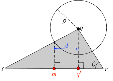
Figure 2: The geometry of a query ball overlapping with a cluster and either one or both of its children.

To determine whether both children can contain points in the query ball, we consider Figure 2. Here, we overload the notation for $\overline{xy}$ to refer to the line segment joining points $x$ and $y$ as well as the length of that line segment.

Let $q$ denote the query, $\rho$ denote the search radius, and $l$ and $r$ denote the cluster’s left and right poles respectively (see Section 2.1.1). Without loss of generality, we assume that $\overline{qr\vphantom{l}}\leq\overline{ql}$. Now let $q^{\prime}$ be the projection of $q$ to $\overline{lr}$, $m$ be the midpoint of $\overline{lr}$, and $d$ be the distance from $q^{\prime}$ to $m$. As a consequence of how we assign a point in the parent cluster to the left child in Algorithm 1, if $q^{\prime}$ is too far from $m$, i.e. $\rho<d$, then when the left child cannot contain points inside the query ball. In such a case we proceed only with the right child. Otherwise, we proceed with both children.

To check whether $d\leq\rho$, we note that

$$d=\overline{mq^{\prime}\vphantom{l}}=\overline{mr\vphantom{l}}-\overline{q^{\prime}r\vphantom{l}}=\frac{\overline{lr}}{2}-\overline{q^{\prime}r\vphantom{l}}.$$

Let $\theta$ denote $\angle lrq$, as shown in Figure 2. By the Law of Cosines on $\triangle lrq$, we have that

$$\text{cos}(\theta)=\tfrac{\overline{lr}^{2}+\ \overline{qr\vphantom{l}}^{2}-\ \overline{ql}^{2}}{2\cdot\overline{lr}\cdot\overline{qr\vphantom{l}}}.$$

Since $\triangle rqq^{\prime}$ is a right triangle, we also have that

$$\text{cos}(\theta)=\tfrac{\overline{q^{\prime}r\vphantom{l}}}{\overline{qr\vphantom{l}}}.$$

Combining the previous two equations and solving for $\overline{q^{\prime}r\vphantom{l}}$, we have that

$$\overline{q^{\prime}r\vphantom{l}}=\tfrac{\overline{qr\vphantom{l}}^{2}+\ \overline{lr}^{2}-\ \overline{ql}^{2}}{2\cdot\overline{lr}}.$$

Substituting for $\overline{q^{\prime}r\vphantom{l}}$ in the equation for $d$, we have that

$$d=\tfrac{\overline{lr}}{2}-\tfrac{\overline{qr\vphantom{l}}^{2}+\ \overline{lr}^{2}-\ \overline{ql}^{2}}{2\cdot\overline{lr}}=\tfrac{\overline{ql}^{2}-\overline{qr\vphantom{l}}^{2}}{2\cdot\overline{lr}}.$$

Thus,

$$d\leq\rho\iff(\overline{ql}+\overline{qr\vphantom{l}})(\overline{ql}-\overline{qr\vphantom{l}})\leq 2\cdot\overline{lr}\cdot\rho.$$ (3)

Note, in particular, that Equation 3 only requires distances between real points, and so it can be used with any distance function, even when $q^{\prime}$ and $m$ are not real points or cannot be imputed from the data.

To perform $\rho$-NN search, we first perform a coarse tree-search, as outlined in Algorithm 2, to find the leaf clusters which overlap with the query ball or any clusters which lie entirely within the query ball. Then, for all such clusters, we perform a finer-grained leaf-search, as outlined in Algorithm 3, to find all points which are no more than a distance $\rho$ from the query.

Algorithm 2 tree-search($C$, $q$, $\rho$)

0:  $C$, a cluster

0:  $q$, a query

0:  $\rho$, a search radius

  if $C$ is a leaf or $\delta^{+}_{C}\leq\rho$ then

     return $\{C\}$

  else

     $[l,r]$ $\Leftarrow$ poles of $C$

     $[L,R]$ $\Leftarrow$ children of $C$

     if $\overline{ql}<\overline{qr\vphantom{l}}$ then

        $[r,l]\Leftarrow[l,r]$

        $[R,L]\Leftarrow[L,R]$

     end if

     if $(\overline{ql}+\overline{qr\vphantom{l}})(\overline{ql}-\overline{qr\vphantom{l}})\leq 2\cdot\overline{lr}\cdot\rho$ then

        return tree-search($L,q,\rho$) $\cup$ tree-search($R,q,\rho$)

     else

        return tree-search($R,q,\rho$)

     end if

  end if

Algorithm 3 leaf-search($S$, $q$, $\rho$)

0:  $S$, a set of clusters

0:  $q$, a query

0:  $\rho$, a search radius

  $H\Leftarrow\emptyset$, a set of hits

  for $C\in S$ do

     if $\delta^{+}_{C}\leq\rho$ then

        $H$ $\Leftarrow$ $H\cup\{C\}$

     else

        for $p\in C$ do

           if $f(p,q)\leq\rho$ then

              $H$ $\Leftarrow$ $H\cup\{p\}$

           end if

        end for

     end if

  end for

  return $H$

Algorithm 4 $\rho$-NN-search($root$, $q$, $\rho$)

0:  $root$, the root cluster

0:  $q$, a query

0:  $\rho$, a search radius

  $S$ $\Leftarrow$ tree-search($root$, $q$, $\rho$)

  $H$ $\Leftarrow$ leaf-search($S$, $q$, $\rho$)

  return $H$

The asymptotic complexity of $\rho$-NN is the same as in [22] and shown in Equation 4.

$$\mathcal{O}\Bigg{(}\underbrace{\log~{}\overbrace{\mathcal{N}_{\hat{r}}(X)}^{\textrm{metric entropy}}}_{\textrm{tree-search}}\ +\ \underbrace{\overbrace{\big{|}B_{X}(q,\rho)\big{|}}^{\textrm{output size}}\overbrace{\left(\frac{\rho+2\cdot\hat{r}}{\rho}\right)^{d}}^{\textrm{scaling factor}}}_{\textrm{leaf-search}}\Bigg{)}$$ (4)

where $\hat{r}$ is the mean radius of leaf clusters, $\mathcal{N}_{\hat{r}}(X)$ is the metric entropy at that radius, $B_{X}(q,\rho)$ is a ball of radius $\rho$ around the query $q$, and $d$ is the LFD around the query at the length scale of $\rho$ and $\rho+2\cdot\hat{r}$.

From Algorithm 4, we have that $H=B_{X}(q,\rho)$, and so $\rho$-NN search performance scales linearly with the size of the output set and exponentially with the LFD around the query. While one might worry that the exponential scaling factor would dominate, the manifold hypothesis suggests that the LFD of real-life datasets is typically very low, and so this algorithm actually scales sub-linearly with the cardinality of the dataset.

2.4 $k$-Nearest Neighbors Search

In this section, we present three novel algorithms for exact $k$-NN search: Repeated $\rho$-NN, Breadth-First Sieve, and Depth-First Sieve.

In these algorithms, we use $H$, for hits, to refer to the data structure which stores the closest points to the query found so far, and $Q$ to refer to the data structure which stores the clusters and points which are still in contention for being one of the $k$ nearest neighbors.

2.4.1 Repeated $\rho$-NN

In this algorithm, we perform $\rho$-NN search starting with a small search radius, and repeatedly increasing the radius until $|H|\geq k$.

Let the search radius $r$ be equal to the radius of the root cluster divided by the cardinality of the dataset. We perform tree-search with radius $r$. If no clusters are found, then we double $r$ and perform tree-search again, repeating until we find at least one cluster. Let $Q$ be the set of clusters returned by the first tree-search which returns at least one cluster.

Now, so long as $\sum_{C\in Q}|C|<k$, we continue to perform tree-search, but instead of doubling $r$ on each iteration, we multiply it by a factor determined by the LFD in the vicinity of the query ball. In particular, we increase the radius by a factor of

$$\min\left(2,\left({\frac{k}{\sum_{C\in Q}|C|}}\right)^{\mu^{-1}}\right)$$ (5)

where $\mu$ is the harmonic mean of the LFD of the clusters in $Q$. We use the harmonic mean to ensure that $\mu$ is not dominated by outlier clusters with very high LFD. We cap the radial increase at 2 to ensure that we do not increase the radius too quickly in any single iteration.

Intuitively, the factor by which we increase the radius should be inversely related to the number of points found so far. When the LFD at the radius scale from the previous iteration is high, this suggests that the data are densely populated in that region. Thus, a small increase in the radius would likely encounter many more points, so a smaller radial increase would suffice to find $k$ neighbors. Conversely, when the LFD at the radius scale from the previous iteration is low, this suggests that the data are sparsely populated in that region. In such a region, a small increase in the radius would likely encounter vacant space, so a larger radial increase is needed. Thus, the factor of radius increase should also be inversely related to the LFD.

Once $\sum_{C\in Q}|C|\geq k$, we are guaranteed to have found at least $k$ neighbors, and so we can stop increasing the radius. We perform $\rho$-NN search with this radius and return the $k$ nearest neighbors.

Algorithm 5 Repeated $\rho$-NN($root$, $q$, $k$)

0:  $root$, the root cluster

0:  $q$, a query

0:  $k$, the number of neighbors to find

  $r\Leftarrow radius$ of the $root$ cluster

  $r\Leftarrow$ $\frac{r}{|root|}$

  loop 

     $Q\Leftarrow$ tree-search($root$, $q$, $r$)

     if $Q\neq\emptyset$ then

        break

     end if

     $r\Leftarrow 2\cdot r$

  end loop

  loop 

     if $\sum_{C\in Q}|C|>=k$ then

        break

     end if

     $\mu\Leftarrow\frac{|S|}{\sum_{C\in Q}\frac{1}{LFD(C)}}$

     $r\Leftarrow r\cdot\min\left(2,\left({\frac{k}{\sum_{C\in Q}|C|}}\right)^{\mu^{-1}}\right)$

     $S\Leftarrow$ tree-search($root$, $q$, $r$)

  end loop

  $H\Leftarrow$ sort($\rho$-NN-search($root$, $q$, $r$))

  return $H[..k]$

2.4.2 Complexity of Repeated $\rho$-NN

The complexity bounds for Repeated $\rho$-NN rely on the assumption that the query point is sampled from the same distribution as the rest of the data or, in other words, that it arises from the same generative process as the rest of the dataset. Given the uses of $k$-NN search in practice, this assumption is reasonable. From this assumption, we can infer that the LFD near the query does not differ significantly from the (harmonic) mean of the LFDs of clusters near the query at the scale of the distance from the query to the $k^{th}$ nearest neighbor.

We find it useful to adopt the terminology used in [22] and [27], and address tree-search and leaf-search separately. Tree-search refers to the process of identifying clusters which have overlap with the query ball, or in other words, clusters which might contain one of the $k$ nearest neighbors. Leaf-search refers to the process of identifying the $k$ nearest neighbors among the points in the clusters identified by tree-search.

In  [22], we showed that the complexity of tree-search is $\mathcal{O}(\log\mathcal{N}_{\hat{r}}(X))$, where $\mathcal{N}_{\hat{r}}(X)$ is the metric entropy of the dataset $X$ at a radius $\hat{r}$. To adjust this bound for Repeated $\rho$-NN, we must estimate the number of iterations of tree-search (Algorithm 2) needed to find a radius that guarantees at least $k$ neighbors.

Based on the assumption that the LFD near the query does not differ significantly from that of nearby clusters, Equation 5 suggests that in the expected case, we need only two iterations of tree-search to find $k$ neighbors: one iteration to find at least one cluster, and the one more to find enough the $k$ neighbors. Since this is a constant factor, complexity of tree-search for Repeated $\rho$-NN is the same as that of $\rho$-NN search, i.e. $\mathcal{O}\big{(}\log\mathcal{N}_{\hat{r}}(X)\big{)}$.

To determine the asymptotic complexity of leaf-search, we must estimate $\sum_{C\in Q}|C|$, the total cardinality of the clusters returned by tree-search. Since we must examine every point in each such clusters, time complexity of leaf-search is linear in $\sum_{C\in Q}|C|$. Let $\rho_{k}$ be the distance from the query to the $k^{th}$ nearest neighbor. Then, we see that $Q$ is expected to be the set of clusters which overlap with a ball of radius $\rho_{k}$ around the query. We can estimate this region as a ball of radius $\rho_{k}+2\hat{r}$, where $\hat{r}$ is the mean radius of the clusters in $Q$.

The work in [27] showed that

$$\sum_{C\in S}|C|\leq\gamma\left|B(q,\rho_{k})\right|\left(\frac{\rho_{k}+2\cdot\hat{r}}{\rho_{k}}\right)^{d}$$

where $\gamma$ is a constant. By definition of $\rho_{k}$, we have that $|B(q,\rho_{k})|=k$. Thus,

$$\sum_{C\in S}|C|\leq\gamma k\left(1+2\cdot\frac{\hat{r}}{\rho_{k}}\right)^{d}$$

An estimate for $\rho_{k}$ is still needed. For this, we once again rely on the assumption that the query is drawn from the same distribution as the rest of the data, and thus the LFD at the query point is not significantly different from the LFD of nearby clusters.

We let $\hat{d}$ be the (harmonic) mean LFD of the clusters in $Q$. While ordinarily we compute LFD by comparing cardinalities of two balls with two different radii centered at the same point, in order to estimate $\rho_{k}$, we instead compare the cardinality of a ball around the query of radius $\rho_{k}$ to the mean cardinality, $\hat{|C|}$, of clusters in $Q$ at a radius equal to the mean of their radii, $\hat{r}$. We justify this approach by noting that, since the query is from the same distribution as the rest of the data, we could move from the query to the center of one of the nearby clusters without significantly changing our estimate of the LFD.

By Equation 1,

$$\hat{d}=\frac{\log{}\frac{\hat{|C|}}{k}}{\log{}\frac{\hat{r}}{\rho_{k}}}$$

We can rearrange this equation to get

$$\frac{\hat{r}}{\rho_{k}}=\left(\frac{\hat{|C|}}{k}\right)^{\hat{d}^{-1}}$$

Using this to simplify the term for leaf-search in Equation 4, we get

$$k\left(1+2\cdot\left(\frac{\hat{|C|}}{k}\right)^{\hat{d}^{-1}}\right)^{d}.$$

In addition, by our assumption that the LFD at the query is not significantly different from the LFD of nearby clusters, we have that $\hat{d}\approx d$. By combining the bounds for tree-search and leaf-search, we see that Repeated $\rho$-NN has an asymptotic complexity of

$$\mathcal{O}\Bigg{(}\underbrace{\log~{}\overbrace{\mathcal{N}_{\hat{r}}(X)}^{\textrm{metric entropy}}}_{\textrm{tree-search}}\ +\ \underbrace{\overbrace{k}^{\textrm{output size}}\overbrace{\bigg{(}1+2\cdot\Big{(}\frac{\hat{|C|}}{k}\Big{)}^{d^{-1}}\bigg{)}^{d}}^{\textrm{scaling factor}}}_{\textrm{leaf-search}}\Bigg{)}$$ (6)

where $\mathcal{N}_{\hat{r}}(X)$ is the metric entropy of the dataset, $d$ is the LFD of the dataset, and $k$ is the number of nearest neighbors. We note that the scaling factor should be close to 1 unless fractal dimension is highly variable in a small region (i.e. if $\hat{d}$ differs significantly from $d$).

2.4.3 Breadth-First Sieve

This algorithm performs a breadth-first traversal of the tree, pruning clusters by using a modified version of the QuickSelect algorithm [35] at each level.

We begin by letting $Q$ be a set of 3-tuples $(p,\delta^{+}_{p},m)$, where $p$ is either a cluster or a point, $\delta^{+}_{p}$ is the $\delta^{+}$ of $p$ as illustrated in Figure 1, and $m$ is the multiplicity of $p$ in $Q$. During the breadth-first traversal, for every cluster $C$ we encounter, we add $(C,\delta^{+}_{C},|C|-1)$ and $(c,\delta_{c},1)$ to $Q$, where $c$ is the center of $C$. Recall that by the definitions of $\delta$ and $\delta^{+}$ given in Section 2.2, since $c$ is a point, $\delta_{C}=\delta_{c}=\delta^{+}_{c}=\delta^{-}_{c}$.

We then use the QuickSelect algorithm, modified to account for multiplicities and to reorder $Q$ in-place, to find the element in $Q$ with the $k^{th}$ smallest $\delta^{+}$; in other words, we find $\tau$, the smallest $\delta^{+}$ in $Q$ such that $\left|B_{X}(q,\tau)\right|\geq k$. Since this step may require a binary search for the correct pivot element to find $\tau$ and reordering with a new pivot is linear-time, this version of QuickSelect may require $\mathcal{O}(|Q|\log|Q|)$ time.

We then remove from $Q$ any element for which $\delta^{-}>\tau$ because such elements cannot contain (or be) one of the $k$ nearest neighbors. Next, we remove all leaf clusters from $Q$ and add their points to $Q$ instead. Finally, we replace all remaining clusters in $Q$ with the pairs of 3-tuples corresponding to their child clusters.

We continue this process until $Q$ no longer contains any clusters. We then use the QuickSelect algorithm once last time to reorder $Q$, find $\tau$, and return the $k$ nearest neighbors.

This process is described in Algorithm 6.

Algorithm 6 Breadth-First Sieve($root$, $q$, $k$)

0:  $root$, the root cluster

0:  $q$, a query

0:  $k$, the number of neighbors to find

  $c\Leftarrow$ center of $root$

  $Q\Leftarrow$ { ($root$, $\delta^{+}_{root}$, $|root|-1$), ($c$, $\delta_{root}$, 1) }

  loop 

     if $k=\sum_{(\_,\_,m)\in Q}m$ then

        break

     end if

     $\tau\Leftarrow$ QuickSelect($Q$, $k$)

     for $(p,\delta^{+}_{p},m)\in Q$ do

        if $\delta^{-}_{p}>\tau$ then

           $Q\Leftarrow Q\setminus\{(p,\delta^{+}_{p},m)\}$

        end if

     end for

     for $(p,\delta^{+}_{p},m)\in Q$ do

        $Q\Leftarrow Q\setminus\{(p,\delta^{+}_{p},m)\}$

        if $p$ is a point then

           continue

        else if $p$ is a leaf then

           for $c\in p$ do

              $Q\Leftarrow Q\cup\{(c,\delta_{c},1)\}$

           end for

        else

           $[L,R]\Leftarrow$ children of $p$

           $Q\Leftarrow Q\cup\{(L,\delta^{+}_{L},|L|-1),(L_{c},\delta_{L},1)\}$

           $Q\Leftarrow Q\cup\{(R,\delta^{+}_{R},|R|-1),(R_{c},\delta_{R},1)\}$

        end if

     end for

  end loop

  return $Q$

2.4.4 Depth-First Sieve

This algorithm performs a depth-first traversal of the tree and uses two priority queues to track clusters and hits.

Let $Q$ be a min-queue of clusters prioritized by $\delta^{-}$ and $H$ be a max-queue (with capacity $k$) of points prioritized by $\delta$. $Q$ starts containing only the root cluster while $H$ starts empty. So long as $H$ is not full or the top priority element in $H$ has $\delta$ greater than or equal to the top priority element in $Q$, we take the following steps:

• While the top priority element $Q$ is not a leaf, remove it from $Q$ and add its children to $Q$.

• Remove the top priority element (a leaf) from $Q$ and add all its points to $H$.

• If $H$ has more than $k$ points, remove points from $H$ until $|H|=k$.

This process is described in Algorithm 7. It terminates when $H$ is full and the top priority element in $H$ has $\delta$ less than the top priority element in $Q$, i.e., the theoretically closest point left to be considered in $Q$ is farther from the query than the $k^{th}$ nearest neighbor in $H$. This leaves $H$ containing exactly the $k$ nearest neighbors to the query.

Algorithm 7 Depth-First Sieve($root$, $q$, $k$)

0:  $root$, the root cluster

0:  $q$, a query

0:  $k$, the number of neighbors to find

  $Q\Leftarrow[root]$, a min-priority queue by $\delta^{-}$

  $H\Leftarrow[]$, a max-priority queue by $\delta$

  while $|H|<k$ or $H.peek.\delta\geq Q.peek.\delta^{-}$ do

     while $\neg(Q.peek$ is a leaf) do

        $C\Leftarrow Q.pop$, the closest cluster

        $[L,R]\Leftarrow$ children of $C$

        $Q.push(L)$

        $Q.push(R)$

     end while

     $leaf\Leftarrow Q.pop$

     for $p\in leaf$ do

        $H.push(p)$

     end for

     while $|H|>k$ do

        $H.pop$

     end while

  end while

  Return $H$

Note that this algorithm is not truly a depth-first traversal of the tree in the classical sense, because we use $Q$ to prioritize which branch of the tree we descend into. Indeed, we expect this algorithm to often switch which branch of the tree is being explored at greater depth.

2.4.5 Complexity of Sieve Methods

We combine the complexity analyses of the two Sieve methods because they are very similar. For these methods we, once again, use the terminology of tree-search and leaf-search. Tree-search navigates the cluster tree and adds clusters to $Q$. Leaf-search exhaustively searches some of the clusters in $Q$ to find the $k$ nearest neighbors.

We start with the assumption that the LFD near the query does not differ significantly from that of nearby clusters, and we consider leaf clusters with cardinalities near $k$. Let $d$ be the LFD in this region. Then the number of leaf-clusters in $Q$ is bounded above by $2d$, e.g. we could have a cluster overlapping the query ball at each end of each of $d$ mutually-orthogonal axes. In the worst-case scenario for tree-search, these leaf clusters would all come from different branches of the tree, and so tree-search looks at $2\cdot d\cdot\log\mathcal{N}_{\hat{r}}(X)$ clusters. Thus, the asymptotic complexity is

$$\mathcal{T}\coloneqq\mathcal{O}\big{(}d\cdot\log\mathcal{N}_{\hat{r}}(X)\big{)}.$$

For leaf-search, the output size and scaling factor are the same as in Repeated $\rho$-NN, and so the asymptotic complexity is

$$\mathcal{L}\coloneqq\mathcal{O}\left(k\cdot\bigg{(}1+2\cdot\Big{(}\frac{\hat{|C|}}{k}\Big{)}^{d^{-1}}\bigg{)}^{d}\right).$$

The asymptotic complexity of Breadth-First Sieve is dominated by the QuickSelect algorithm to calculate $\tau$. Since this method is log-linear in the length of $Q$, and $Q$ contains the clusters from tree-search and the points from leaf-search, we see that the asymptotic complexity is

$$\mathcal{O}\Big{(}(\mathcal{T}+\mathcal{L})\log(\mathcal{T}+\mathcal{L})\Big{)}.$$ (7)

For Depth-First Sieve, since we use two priority queues, the asymptotic complexity is dominated by the complexity of the priority queue operations. Thus, the asymptotic complexity is

$$\mathcal{O}\Big{(}\mathcal{T}\log\mathcal{T}+\mathcal{L}\log k\Big{)}.$$ (8)

2.5 Auto-Tuning

We perform some naïve auto-tuning to select the optimal $k$-NN algorithm to use with a given dataset. We start by taking the center of every cluster at a low depth, e.g. 10, in the cluster tree as a query. This gives us a small, representative sample of the dataset. Using these clusters’ centers as queries, and a user-specified value of $k$, we record the time taken for $k$-NN search on the sample using each of the three algorithms described in Section 2.4. We select the fastest algorithm over all the queries as the optimal algorithm for that dataset and value of $k$. Note that even though we select the optimal algorithm based on use with some user-specified value of $k$, we still allow search with any value of $k$.

2.6 Synthetic Data

Based on our asymptotic complexity analyses, we expect CAKES to perform well on datasets with low LFD, and for its performance to scale sub-linearly with the cardinality of the dataset. To test this hypothesis, we use some datasets from the ANN-benchmarks suite [14] and synthetically augment them to generate similar datasets with exponentially larger cardinalities. We do the same with a large random dataset of uniformly distributed points in a hypercube. We then compare the performance of CAKES to that of other algorithms on the original datasets and the synthetically augmented datasets.

To elaborate on the augmentation process, we start with an original dataset from the ANN-benchmarks suite. Let $X$ be the dataset, $d$ be its dimensionality, $\epsilon$ be a user-specified noise level and $m$ be a user-specified integer multiplier. For each datum $x\in X$, we create $m-1$ new data points within a distance $\epsilon\cdot||x||$ of $x$ where $||x||$ is the Euclidean distance from $x$ to the origin. We construct a random vector $r$ of $d$ dimensions in the hyper-sphere of radius $\epsilon$ centered at the origin. We then add $r$ to $x$ to get a new point $x^{\prime}$. Since $||r||\leq\epsilon$, we have that $||x-x^{\prime}||\leq\epsilon$ (i.e., $x^{\prime}$ is within a distance $\epsilon$ of $x$). This produces a new dataset $X^{\prime}$ with $|X^{\prime}|=m\cdot|X|$.

This augmentation process preserves the topological structure of the original dataset, but increases its cardinality by a factor of $m$, allowing us to isolate the effect of cardinality on search performance from that of other factors such as dimensionality, choice of metric, or the topological structure of the dataset.

3 Datasets And Benchmarking

3.1 ANN-Benchmark Datasets

We benchmark on a variety of datasets from the ANN-benchmarks suite [36], using the associated distance function. Table 1 summarizes the properties of these datasets.

The benchmarks for Fashion-Mnist, Glove-25, Sift, and Random (and for their synthetic augmentations) were conducted on an Amazon AWS (EC2) r6i.16xlarge instance, with a 64-core Intel Xeon Platinum 8375C CPU 2.90GHz processor, 512GB RAM. This is the same configuration used in [36]. The OS kernel was Ubuntu 22.04.3-Ubuntu SMP. The Rust compiler was Rust 1.72.0, and the Python interpreter version was 3.9.16.

The benchmarks for SILVA and RadioML were conducted on an Intel Xeon E5-2690 v4 CPU @ 2.60GHz with 512GB RAM. The OS kernel was Manjaro Linux 5.15.130-1-MANJARO. The Rust compiler was Rust 1.72.0, and the Python interpreter version was 3.9.16.

Table 1: Datasets used in benchmarks.

Dataset	Distance	Cardinality	Dimensionality
Fashion-Mnist	Euclidean	60,000	784
Glove-25	Cosine	1,183,514	25
Sift	Euclidean	1,000,000	128
Random	Euclidean	1,000,000	128
SILVA	Levenshtein	2,224,640	3,712 - 50,000
RadioML	Dynamic Time Warping	97,920	1,024

3.2 Random Datasets and Synthetic Augmentations

In addition to benchmarks on datasets from the ANN-Benchmarks suite, we also benchmarked on synthetic augmentations of these real datasets, using the process described in 2.6. In particular, we use a noise tolerance $\epsilon=0.01$ and explore the scaling behavior as the cardinality multiplier (referred to as “Multiplier” in Table 2) increases.

We also benchmarked on purely random (i.e., not an augmented version of a known dataset), datasets of various cardinalities. For this, we used a base cardinality of 1,000,000 and a dimensionality of 128 to match the Sift dataset; hereafter, we refer to the random dataset with cardinality 1,000,000 and dimensionality 128 as “Random.” This benchmark allows us to isolate the effect of a manifold structure (which we expect to be absent in a purely random dataset) on the performance of the CAKES’ algorithms.

3.3 SILVA 18S

To showcase the use of CAKES with a more exotic distance function, we also benchmarked on the SILVA 18S ribosomal DNA dataset [8]. This dataset contains ribosomal DNA sequences of 2,224,640 genomes with an aligned length of 50,000 letters. We held out a set of 1,000 random sequences from the dataset to use as queries for benchmarking. We use Levenshtein [24] distance on the unaligned sequences to build the tree and to perform $k$-NN search. Since this dataset contains many redundant, i.e. nearly identical, sequences, we used a maximum tree-depth of 128 as a partition criterion in Algorithm 1.

3.4 Radio ML

To provide another example of use of CAKES with a more exotic distance function, we benchmarked on the RadioML dataset [9]. The RadioML dataset contains samples of synthetically generated signal captures of different modulation modes over a range of SNR levels. Specifically, it is comprised of 24 modulation modes at 26 different SNR levels ranging from -20 dB to 30 dB, with 4,096 samples at each combination of modulation mode and SNR level. Thus, it contains $24\cdot 26\cdot 4096=2,555,504$ samples in total. Each sample is a 1,024-dimensional complex-valued vector, representing a signal capture (a time-series of complex-valued numbers). We used a subset of this dataset, containing 97,920 samples at 10dB SNR and used the other 8,576 samples at 10dB SNR as a hold-out set of queries. We use Dynamic Time Warping [33] as the distance function for this dataset.

3.5 Other Algorithms

We benchmarked CAKES’s algorithms against the state-of-the-art similarity search algorithms HNSW, ANNOY and FAISS-IVF, and two implementations of linear search. In particular, we use FAISS-Flat, a Python implementation of linear search, to provide ground-truth values for recall of HNSW, ANNOY, and FAISS-IVF. We use our own Rust implementation of linear search to provide ground-truth values for calculating recall of CAKES’s algorithms. We plot the throughput of these two implementations of linear search as a reference point for all other algorithms in Figures 5

4 Results

4.1 Local Fractal Dimension of Datasets

Since the time complexity of CAKES algorithms scales with the LFD of the dataset, we examine the LFD of each dataset we used for benchmarks.

Figure 3 illustrates the trends in LFD for (the non-augmented versions of) Fashion-Mnist, Glove-25, Sift, Random, Silva 18S, and RadioML. The horizontal axis denotes the depth in the cluster tree, and the vertical axis denotes the LFD (as calculated by Equation 2) of clusters at that depth. We plot lines for the 5^th, 25^th, 50th, 75^th and 95^th percentiles of LFD, as well as the minimum and maximum LFD at each depth. In order to have the plots to best reflect the distribution of LFDs across the entire dataset, we compute percentiles counting each cluster as many times as its cardinality. In other words, if, for some dataset, the 95^th percentile of LFD at depth 40 is 3, this means that 95% of the total points in clusters at depth 40 belong to clusters whose LFD is at most 3.

Figure 3(a) shows the LFD by depth for Fashion-Mnist. We observe that until about depth 5, the LFD is low, as the 95^th percentile (orange plotted line) is less than 4, and the median (red line) is just above 2. For depths 15 through 25, we observe that the LFD increases, with the 95^th percentile (orange plotted line) slightly less than 6, and the median near 3. Finally, for depths 25 through the maximum depth, we observe that the LFD decreases again, as the 95^th percentile is between 3 and 4, and the median is less than 2.

Relative to Fashion-Mnist, Glove-25 has low LFD, as shown in Figure 3(b). Percentile lines for Glove-25 are flatter and lower, indicating that the LFD is lower across the entire dataset, and that the LFD does not vary as much by depth. The 95^th percentile of LFD is less than 3 for all depths, and the median is less than 2 for all depths. Before depth 25, the 95^th percentile hovers near 2, and from depth 20 onward, it hovers near 3.5 before dipping sharply at the maximum depths. The median hovers near 1.5 for all depths.

Figure 3(c) shows the LFD by depth for Sift. Until about depth 5, the 95^th percentile is between 2 and 6. From about depth 5 through about depth 20, the 95^th percentile is greater than 6, even exceeding 8 near depth 10. From about depth 20 onward, the 95^th percentile is less than 6, and from about depth 30 onward, it is between 3 and 4. The median reaches its peak of about 5 at around depth 15, but hovers near 2 after about depth 30.

In contrast with Figure 3(c), Figure 3(f) shows the LFD by depth for a random dataset with the same cardinality and dimensionality as those of Sift. We observe that the LFD starts as high as 20 (for all data) at depth 0. As shown by the needlepoint shape of the plot, the LFD for all clusters has a very narrow spread from depth 0 through depth 5. After depth 5, we begin to see a wider spread between the maximum and minimum LFD at each depth. All percentile lines seem to decrease linearly with depth. The LFD of approximately 20 at depth 0 (i.e. the root cluster) is what we expect for this random dataset. To elaborate, the distribution of points in such a dataset should reflect the curse of dimensionality, i.e. the fact that in high dimensional spaces, the minimum and maximum pairwise distances between any two points are approximately equal. As a result, the root cluster’s radius $r$, which reflects the maximum distance between the center $c$ and any other point, should not differ significantly from the distance between the center and its closest point. A consequence of this is that, with high probability, every point in the root cluster is farther away from the center than half the radius of the root cluster; $B_{X}(c,\tfrac{r}{2})$ contains only $c$ while $B_{X}(c,r)$ contains the entire dataset. Given our definition of LFD in Equation 1, this means that the LFD of the root cluster is approximately $\log_{2}(\frac{|X|}{1})=\log_{2}(1,000,000)\approx 20$, which is what we observe in Figure 3(f).

Silva, as shown in Figure 3(e), exhibits consistently low LFD. The 95^th percentile is less than about 3 for all depths, hovering near 1 for depths 40 through 128. The median reaches its peak at 2 for about depth 10 and remains close to 0 for depths 40 through 128.

Relative to the other datasets, RadioML, as displayed in Figure 3(d), exhibits high LFD. Notably, however, for the first approximately 15 depths, the 95^th percentile and median LFD are very close to 0. Both percentiles increase sharply after depth 20, nearly reaching 16. LFD remains high even as depth increases, with the 95^th percentile fluctuating between about 6 and 15 for depths about 20-40. It then spikes up again to about 10 at around depth 45 before decreasing linearly to 1 at depth 60. The median LFD follows a similar pattern of peaks and troughs, fluctuating between about 3 and 15 for depths 20-40, spiking at about depth 50 to 5, and then decreasing approximately linearly to 1 at depth 60.

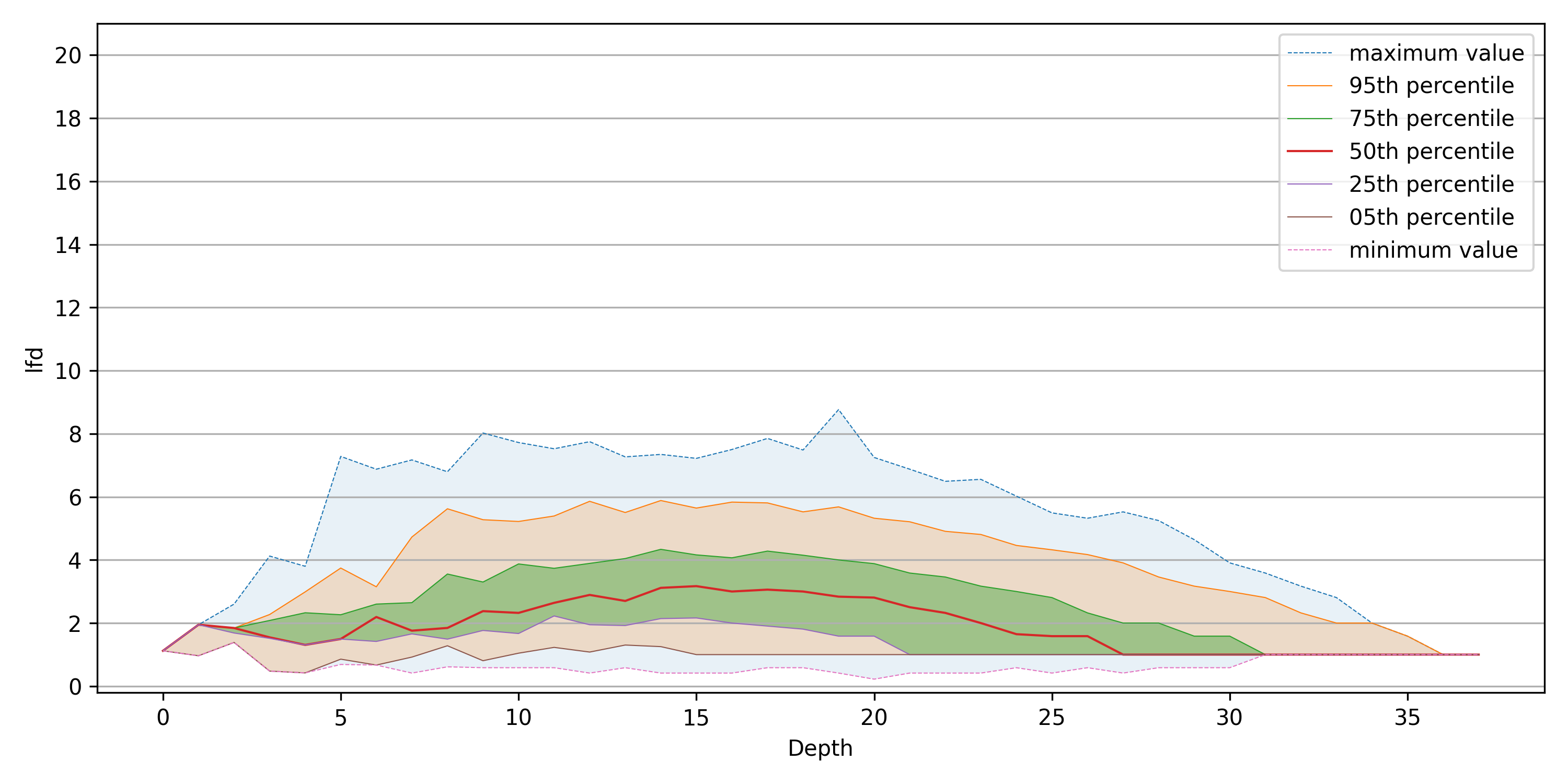
(a) Fashion-mnist

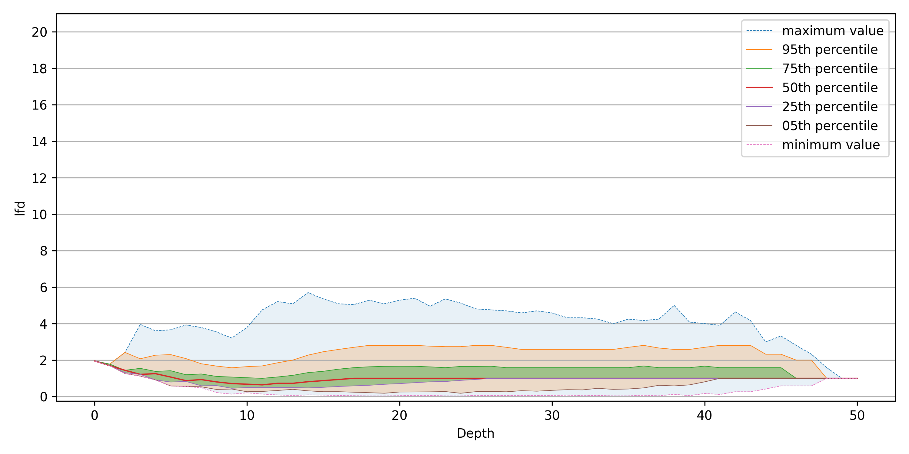
(b) Glove-25

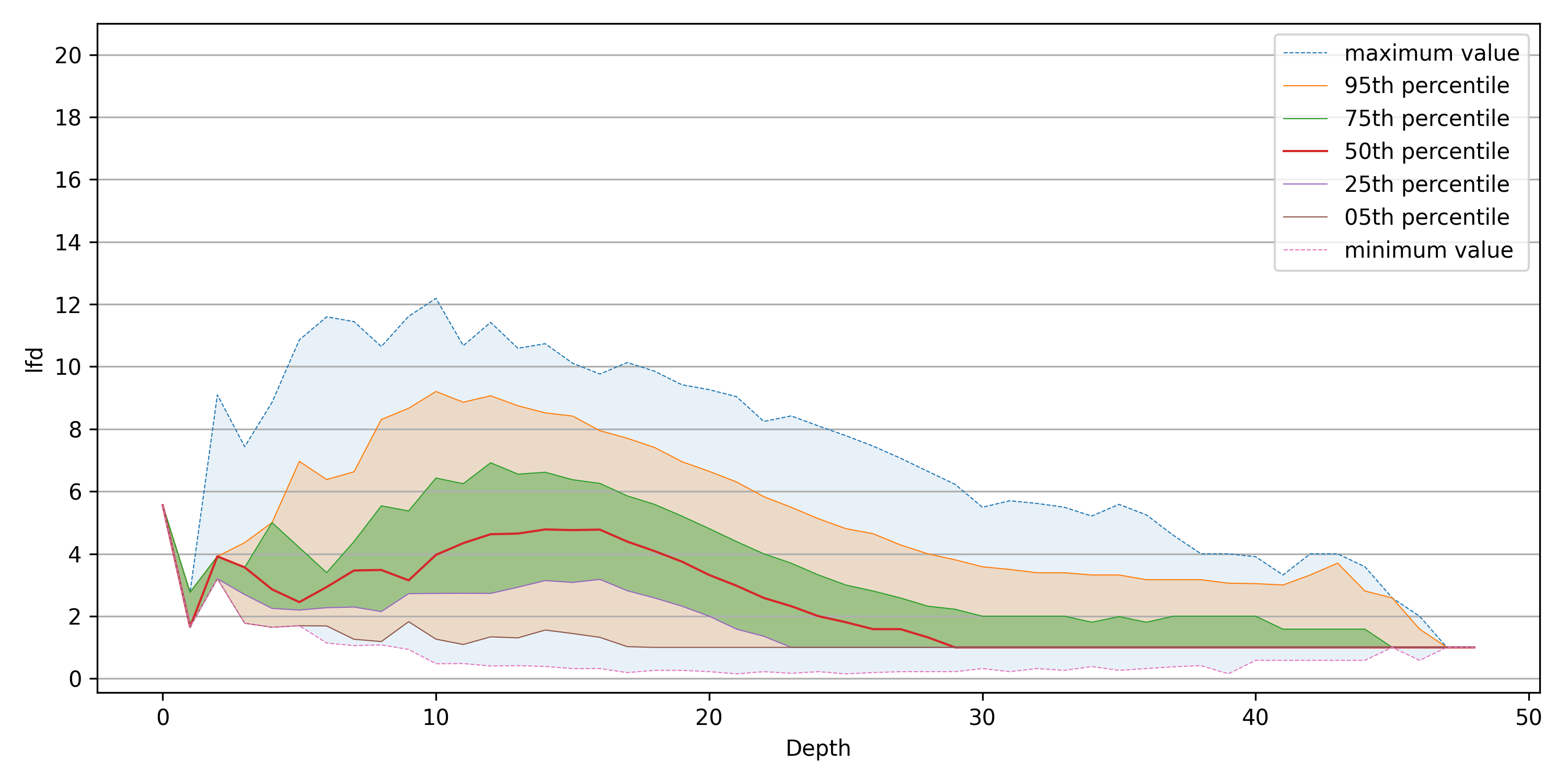
(c) Sift

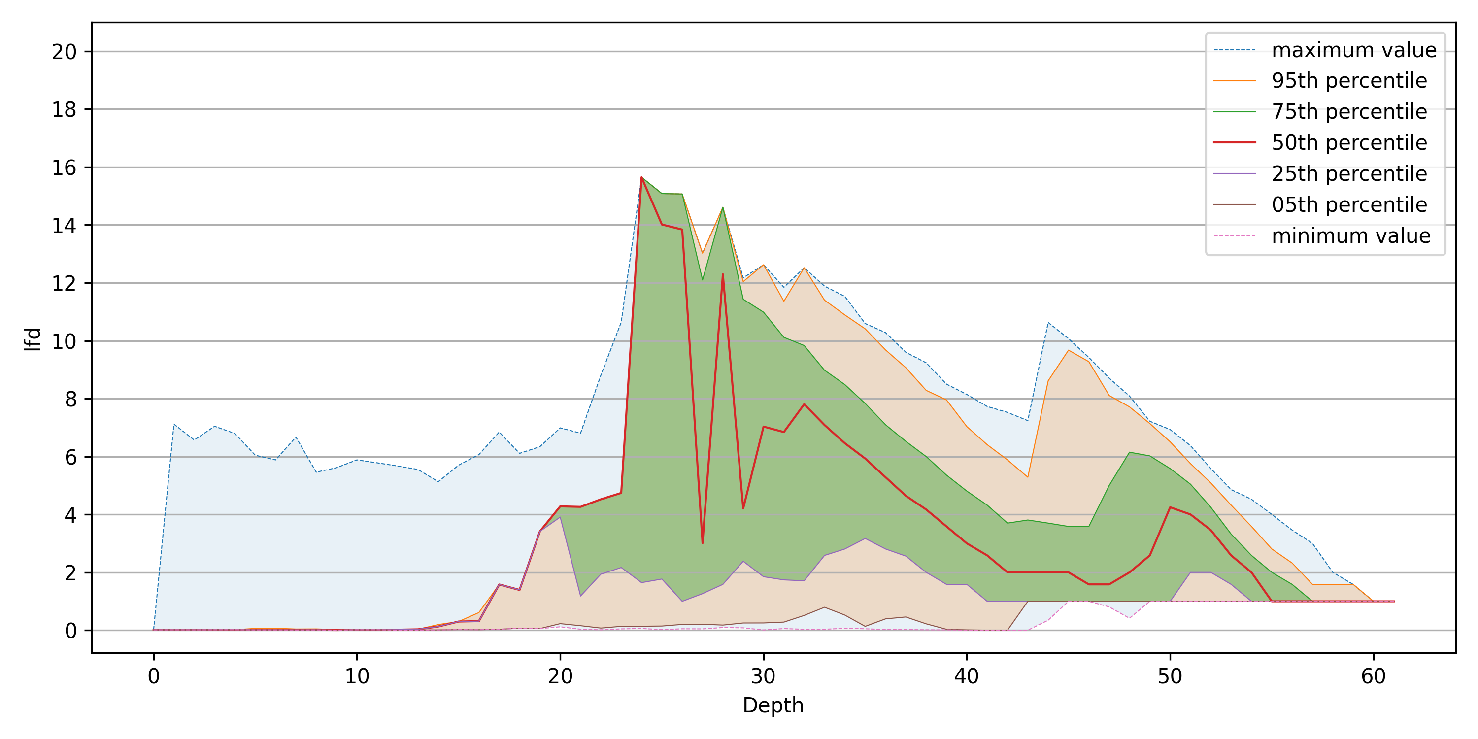
(d) RadioML

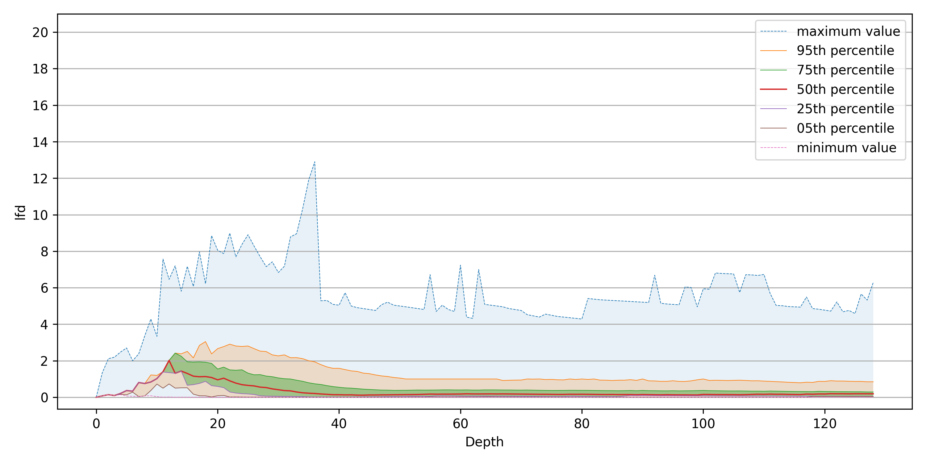
(e) Silva 18S

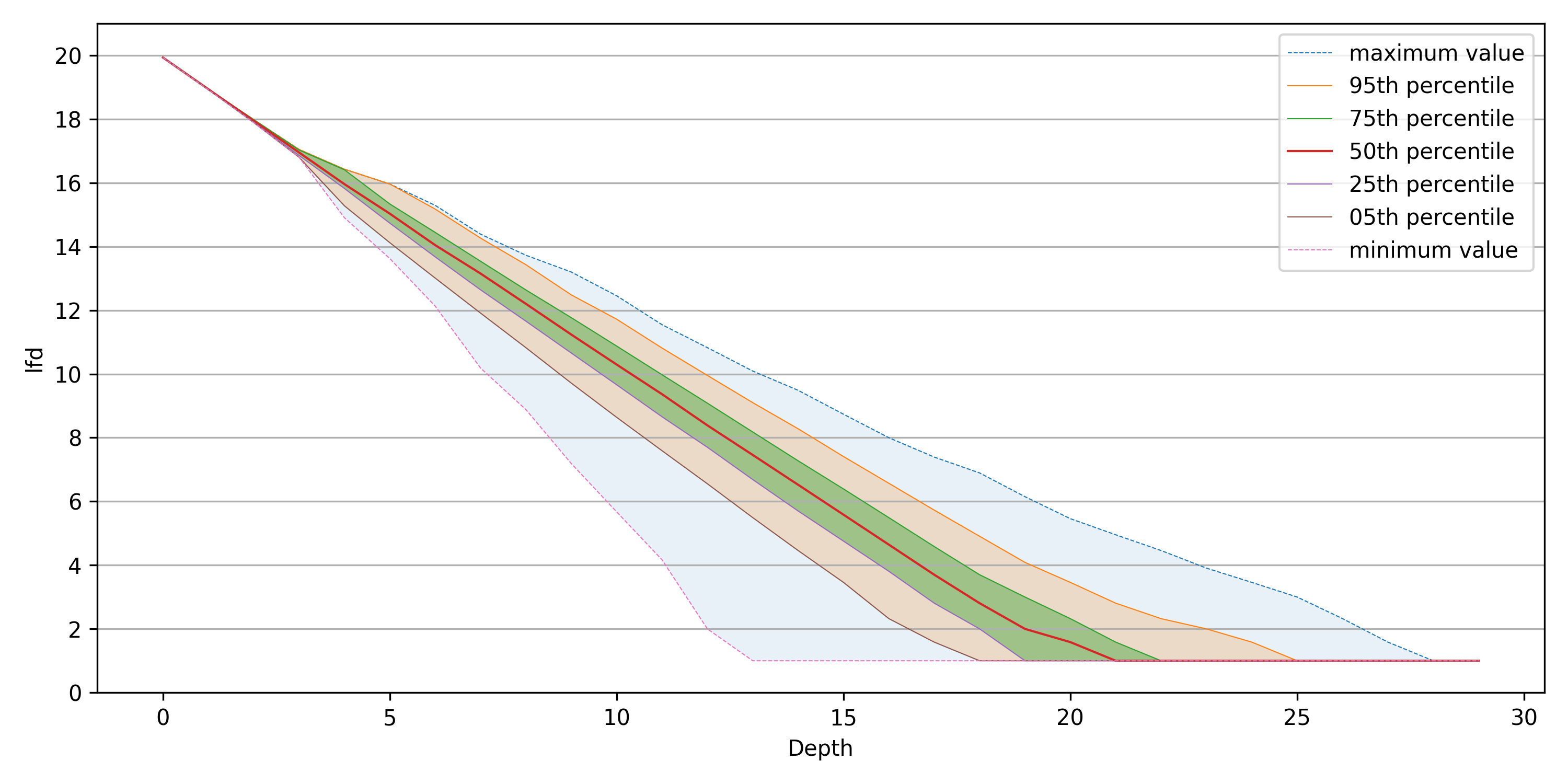
(f) A random dataset

Figure 3: Local fractal dimension vs. cluster depth across six datasets, grouped by decile of local fractal dimension and weighted by the cardinalities of the clusters. The last dataset is randomly generated.

4.2 Indexing and Tuning Time

For each of the ANN-benchmark datasets and the Random dataset, we report the time taken for each algorithm to build the index and to tune the hyper-parameters for these indices to achieve the highest possible recall. Though CAKES has three different algorithms, they share the same tree and so they have the same indexing time. Thus, we show CAKES’s indexing time only once.

The plots in Figure 4 show the results of these benchmarks. The horizontal axis in each subplot shows the cardinality of the dataset augmented with synthetic points (see Section 2.6). The left-most point on each line is at the cardinality of the original dataset without any synthetic augmentation. The vertical axis denotes the sum of indexing and tuning time in seconds. Both axes are on a logarithmic scale. Hereafter, when we refer to the “indexing time” of an algorithm, we are implicitly referring to the sum of indexing and tuning time for said algorithm.

On all datasets, we observe that the indexing time for CAKES increases roughly linearly as cardinality increases. HNSW and ANNOY have the slowest indexing times across all the algorithms we benchmarked for each of the four datasets, at each cardinality. On some datasets, HNSW and ANNOY exhibit indexing times which are orders of magnitude slower than that of CAKES. FAISS-Flat also exhibits the fastest indexing time on each dataset. This is not surprising, given that FAISS-Flat is a naive linear search algorithm and is not building an index.

We also highlight some differences in indexing time between different datasets. With Fashion-Mnist, as shown in Figure 4(a), we observe that the indexing time for CAKES is lower than that of FAISS-IVF for all cardinalities. With Glove-25 (see Figure 4(b)), however, at cardinalities greater than $10^{7}$, FAISS-IVF has lower indexing time than CAKES. With Sift, CAKES’s indexing time is faster than that of FAISS-IVF until a cardinality of nearly $10^{8}$, and with the Random dataset, we observe that CAKES has faster indexing time than FAISS-IVF until a cardinality of nearly $10^{7}$.

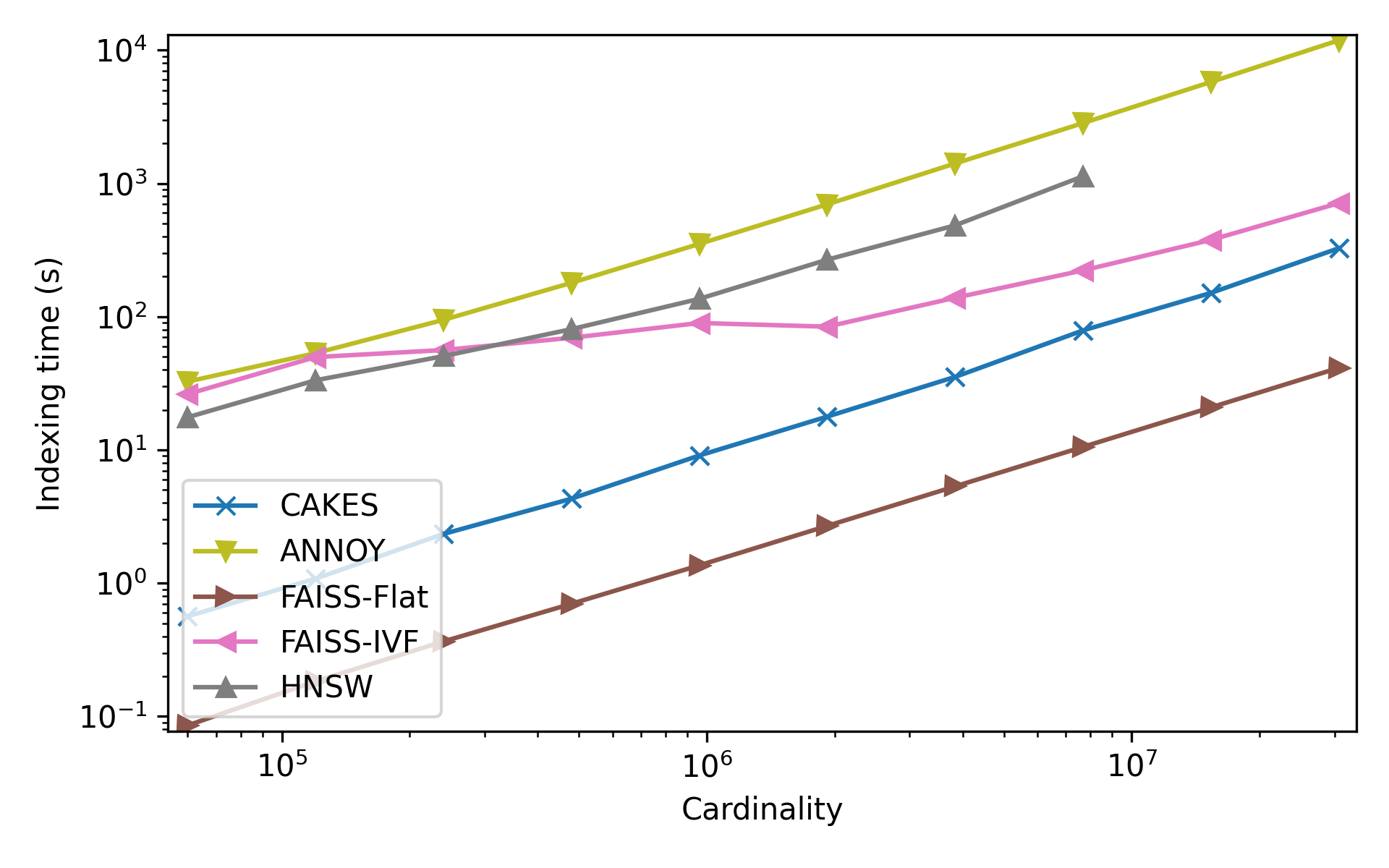
(a) Fashion-mnist

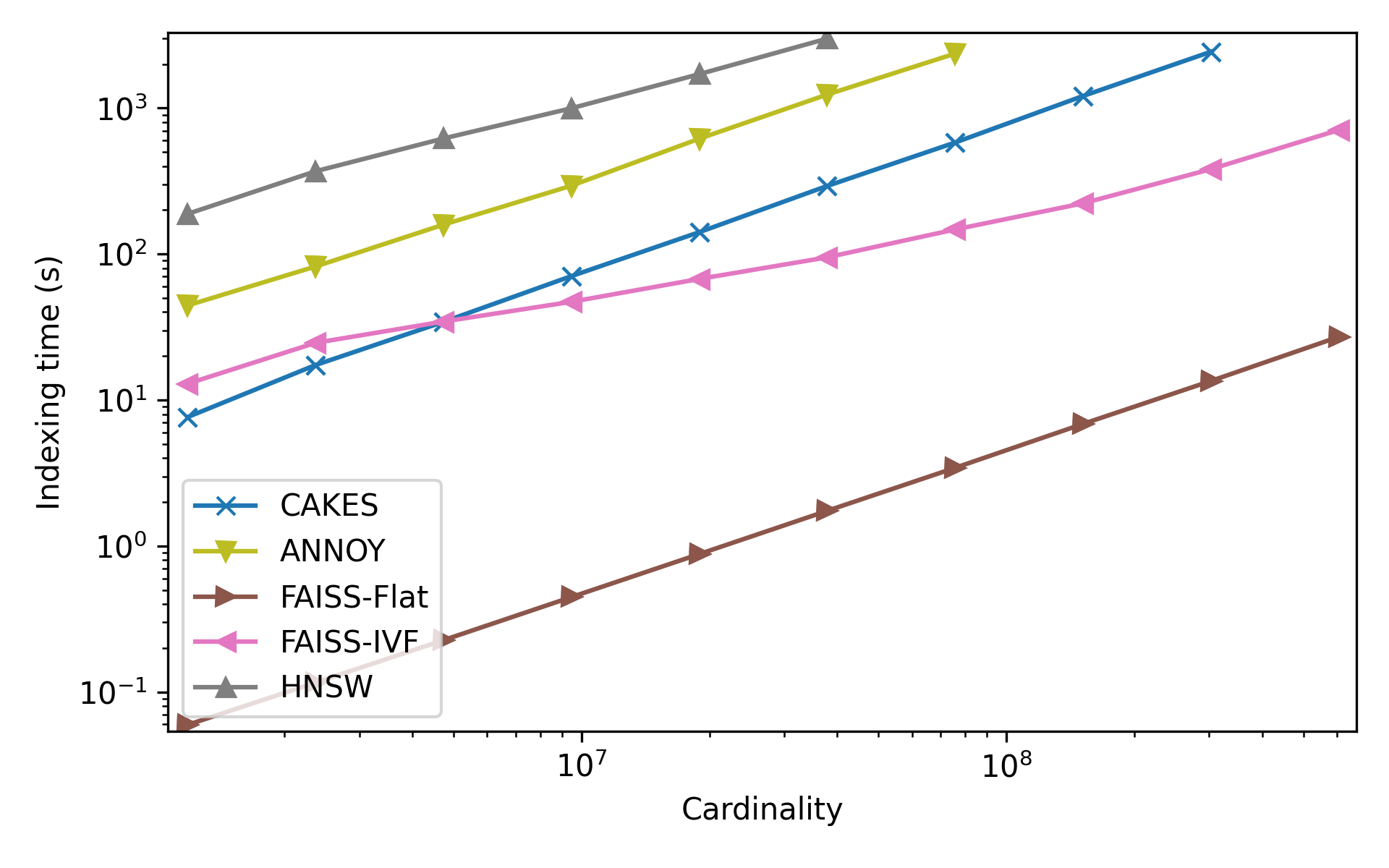
(b) Glove-25

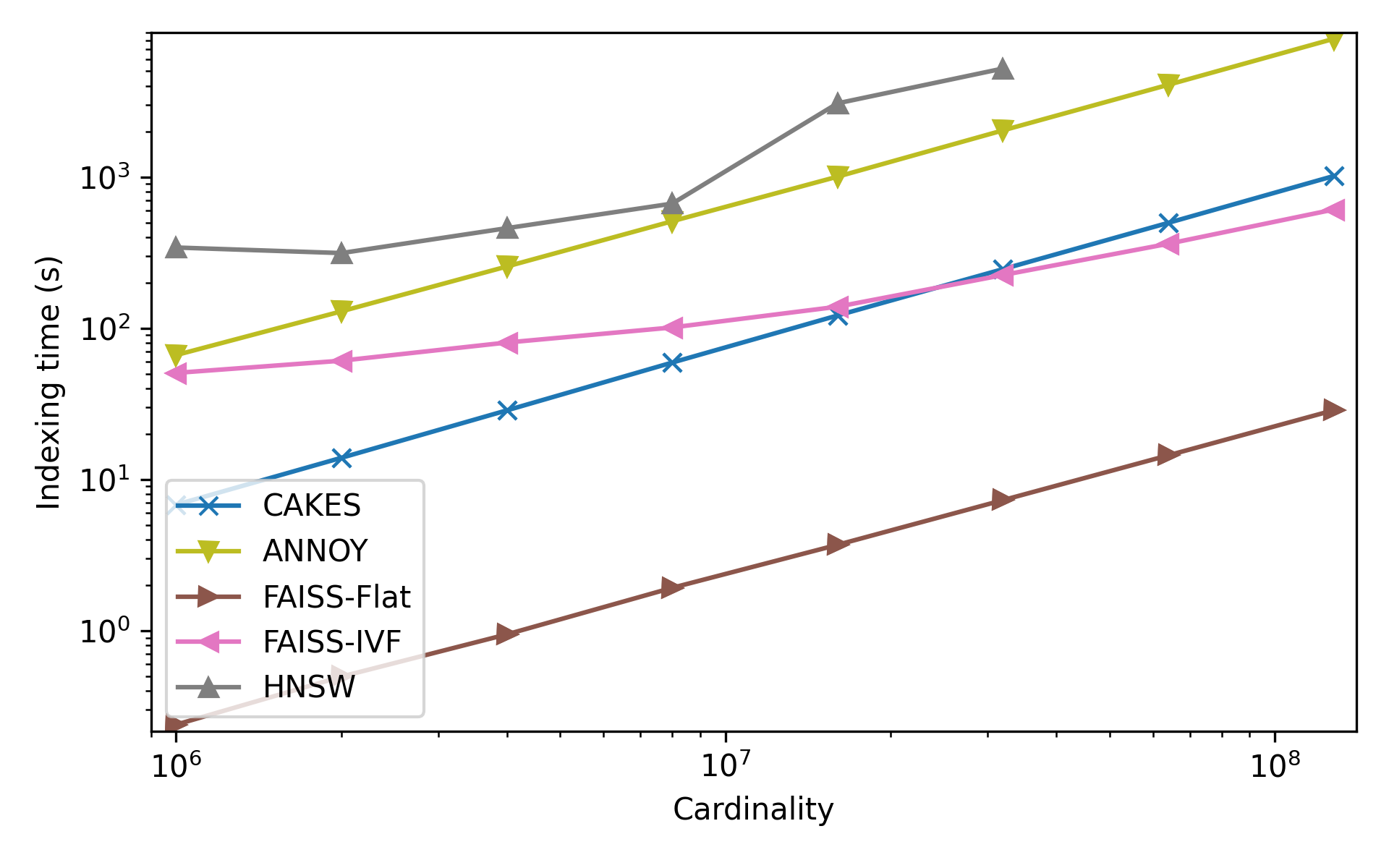
(c) Sift

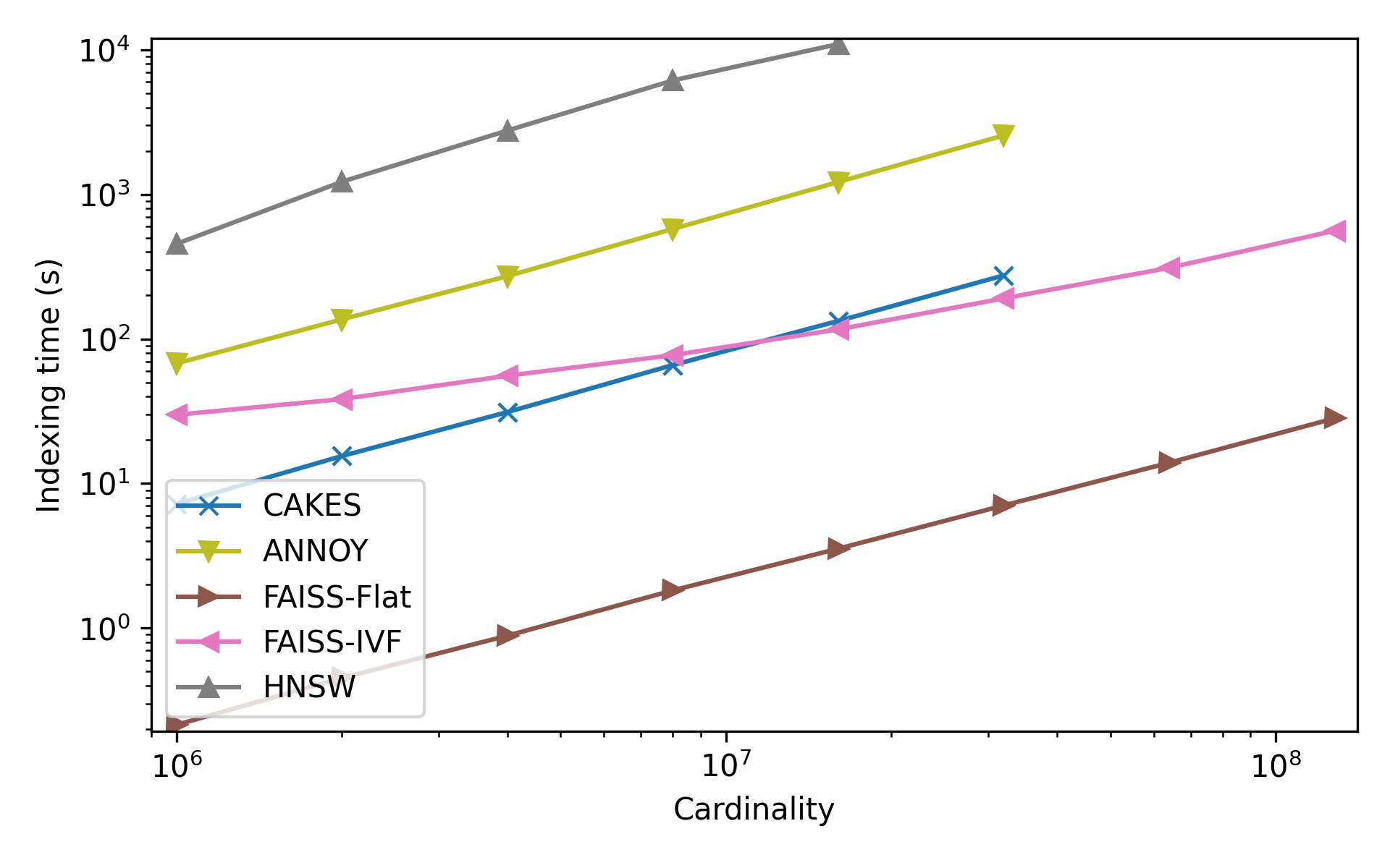
(d) Random

Figure 4: Indexing and tuning time for each algorithm with each of the ANN benchmark datasets and the Random dataset.

4.3 Scaling Behavior and Recall

Figures 5(a), 5(b), and 5(c) show the scaling behavior of CAKES algorithms and existing algorithms on augmented versions of the following ANN-benchmark datasets:

• Fashion-Mnist under Euclidean distance,

• Glove-25 under Cosine distance, and

• Sift under Euclidean distance.

Figure 5(f) shows the scaling behavior of CAKES algorithms and existing algorithms on a completely randomly generated dataset with same cardinality and dimensionality as Sift (1 million points in 128 dimensions). Figures 5(e) and  5(d) show the scaling behavior of CAKES on Silva and RadioML respectively. For these datasets, we took random sub-samples of the full datasets instead of augmenting them to higher cardinalities.

The horizontal axis in each figure shows the cardinality of the augmented dataset with synthetic points (see Section 2.6). The left-most point on each line is at the cardinality of the original dataset without any synthetic augmentation. The vertical axis denotes throughput in queries per second. Both axes are on a logarithmic scale. In this section, we report results only for $k$-NN search with $k=10$, but similar plots for $k=100$ can be found in the Supplement. For HNSW and ANNOY, we report the recall for each measurement in the plots. For algorithms which exhibit recall greater than $0.9995$, we do not report the recall in the plots, but we do report it in the tables below.

Table 2 show the throughput and recall of CAKES’s algorithms at each augmented cardinality for Fashion-Mnist, Glove-25, Sift, and Random. Though the plots in Figure 5 present results for each of CAKES’s three algorithms separately, the results in the CAKES column in these tables represent the fastest CAKES algorithm at that dataset and cardinality only. We used our auto-tuning approach (see Section 2.5) for each new tree (i.e. at each cardinality), and this approach was always able to select the fastest algorithm for each dataset at each cardinality. Since we also allow for tuning hyper-parameters for the other algorithms, and we allow for different sets of hyper-parameters at each cardinality, it is a fair comparison for these tables to only list the performance of the tuned CAKES algorithm. When reporting recall, we use $1.000*$ to denote that the recall is imperfect, but rounds to $1.000$ when we consider only three decimal places.

Figure 5 shows that for Fashion-Mnist, Glove-25, and Sift, as cardinality increases, the CAKES algorithms (Depth-First Sieve in blue, Repeated $\rho$-NN in green, and Breadth-First Sieve in purple) become faster than our Rust implementation of naïve linear search (in orange). Though we observe this trend, we note that the exact cardinality at which CAKES’s algorithms overtake linear search differs by dataset. For Fashion-Mnist, CAKES begins exhibiting sub-linear performance starting at a cardinality near $10^{5}$, while for Glove-25 and Sift, this happens near $10^{6}$ and $10^{7}$ respectively. Which one of the three CAKES algorithms is fastest also differs by dataset. For Fashion-Mnist, Depth-First Sieve is consistently fastest, while for Glove-25, the fastest is Repeated $\rho$-NN, and for Sift, Breadth-First Sieve. Additionally, on all three datasets, Depth-First Sieve and Breadth-First Sieve appear to have performance which is constant in the cardinality of the dataset. With Glove-25, Repeated $\rho$-NN exhibits similar constant scaling. We also observe that on these three datasets, for nearly all cardinalities, all three of the CAKES algorithms are faster than FAISS-Flat (in brown), and that at some cardinality, CAKES’s algorithms become faster than FAISS-IVF (in pink). For Fashion-Mnist, CAKES becomes faster than FAISS-IVF near cardinality $10^{5}$, whereas for Glove-25 and Sift, this happens near cardinality $10^{7}$. On all three of these datasets, HNSW (in gray) and ANNOY (in yellow) are faster than CAKES’s algorithms for all cardinalities; however, CAKES exhibits perfect or near-perfect recall on each dataset, while HNSW and ANNOY exhibit much lower recall, as shown in Table 1. While recall for CAKES’s algorithms does not degrade with cardinality, recall for HNSW and ANNOY does degrade with cardinality. At a cardinality multiplier as low as eight, HNSW and ANNOY have recall of $0.525$ and $0.857$ respectively for Fashion-Mnist, 0.607 and 0.832 for Glove-25, and 0.782 and 0.686 on Sift. In contrast, CAKES has perfect recall on Fashion-Mnist and Sift (because the distance function used with these datasets is a metric), and near-perfect recall on Glove-25 (because the Cosine distance function is not a metric).

In contrast with the results on the ANN Benchmark datasets reported above, with the Random dataset, as seen in Figure 5(f), we observe that the three CAKES algorithms are the slowest out of all algorithms, at all cardinalities. As with the real datasets, HNSW and ANNOY are the fastest algorithms, and CAKES exhibits perfect recall at all cardinalities. HNSW and ANNOY exhibit much lower recall on this random dataset than on any of the ANN benchmark datasets; in particular, with a multiplier of 1, HNSW and ANNOY have recall as low as 0.060 and 0.028 respectively, as reported in Table 2.

For Silva and RadioML, we benchmarked only CAKES’s algorithms because HNSW, ANNOY and FAISS do not support neither the required distance functions nor, in the case of RadioML, complex-valued data. Due to the massive sizes of these datasets, we took random sub-samples of the dataset with lower cardinalities for our benchmarks, rather than augmented versions of the dataset. With Silva, as shown in Figure 5(e), we observe that for all algorithms, throughput seems to linearly decrease as cardinality increases, but that it seems to begin levelling off near cardinality $10^{5}$. Until cardinality near $10^{4}$, Depth-First Sieve is the fastest CAKES algorithm, but for larger cardinalities, Repeated $\rho$-NN is the fastest CAKES algorithm. For RadioML, as shown in Figure 5(d), we observe that throughput declines nearly linearly the three CAKES algorithms exhibit nearly indistinguishable performance for all cardinalities. In particular, throughput of CAKES’s algorithms is identical within three significant figures for all cardinalities.

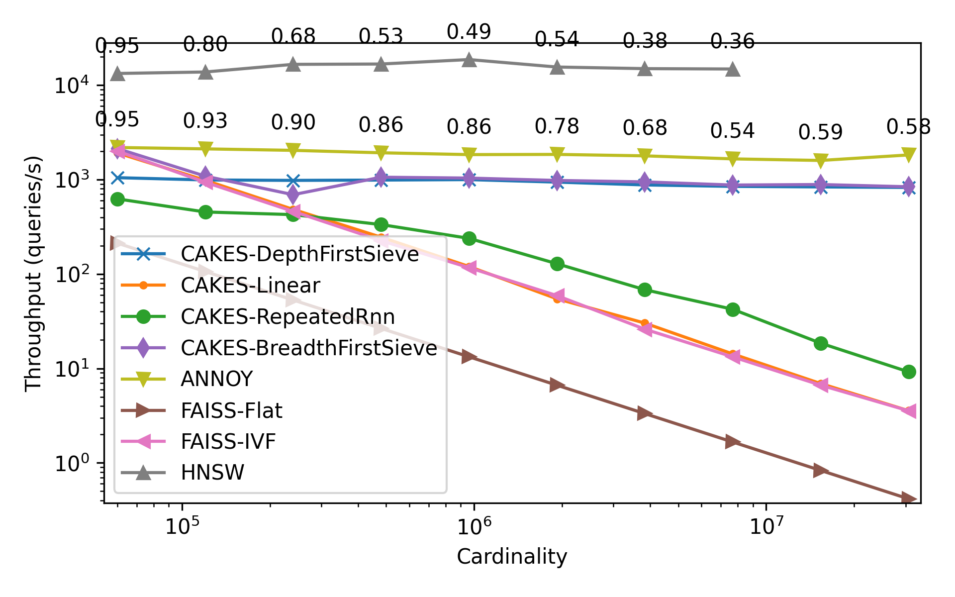
(a) Fashion-Mnist for $k=10$.

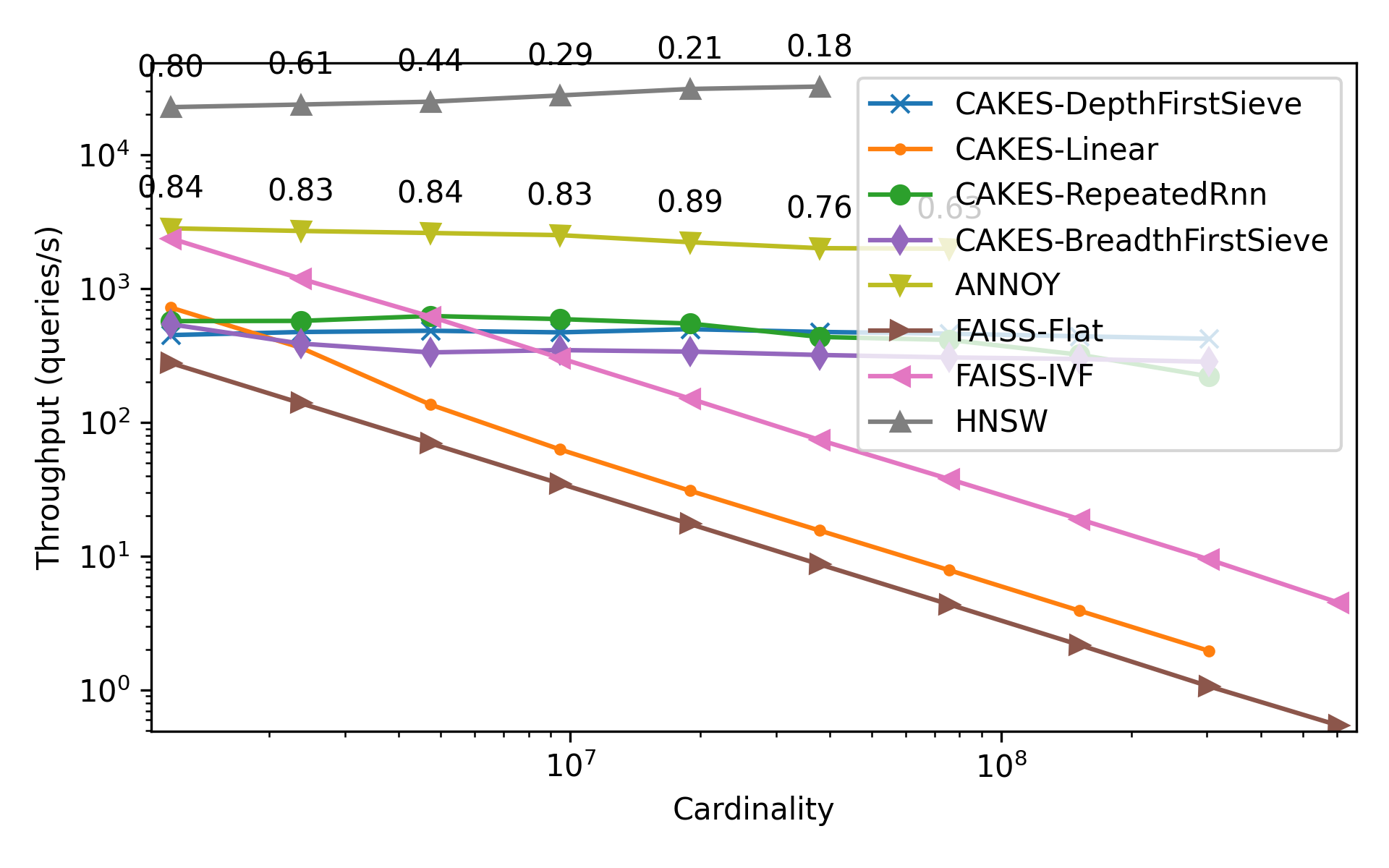
(b) Glove-25 for $k=10$.

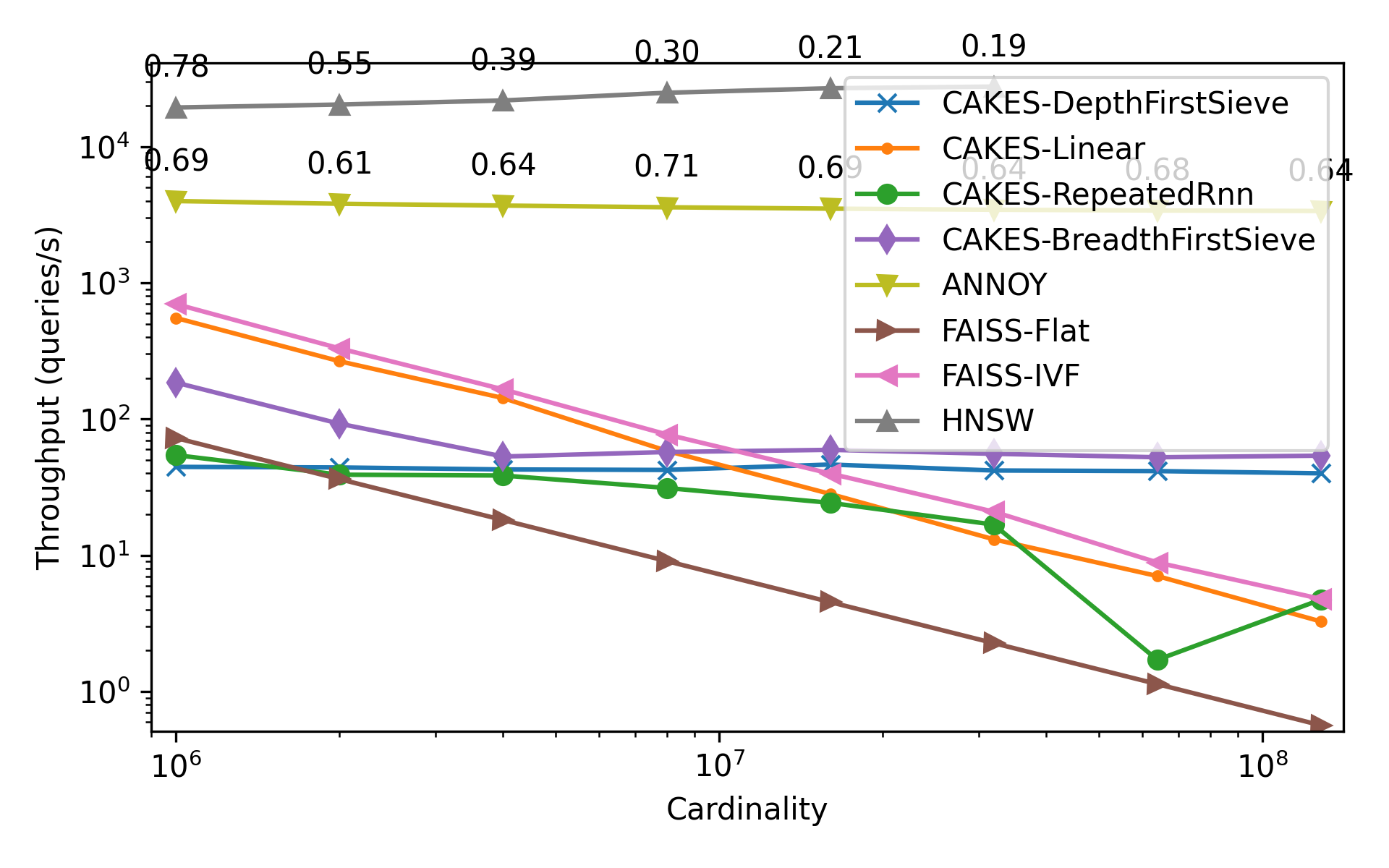
(c) Sift for $k=10$.

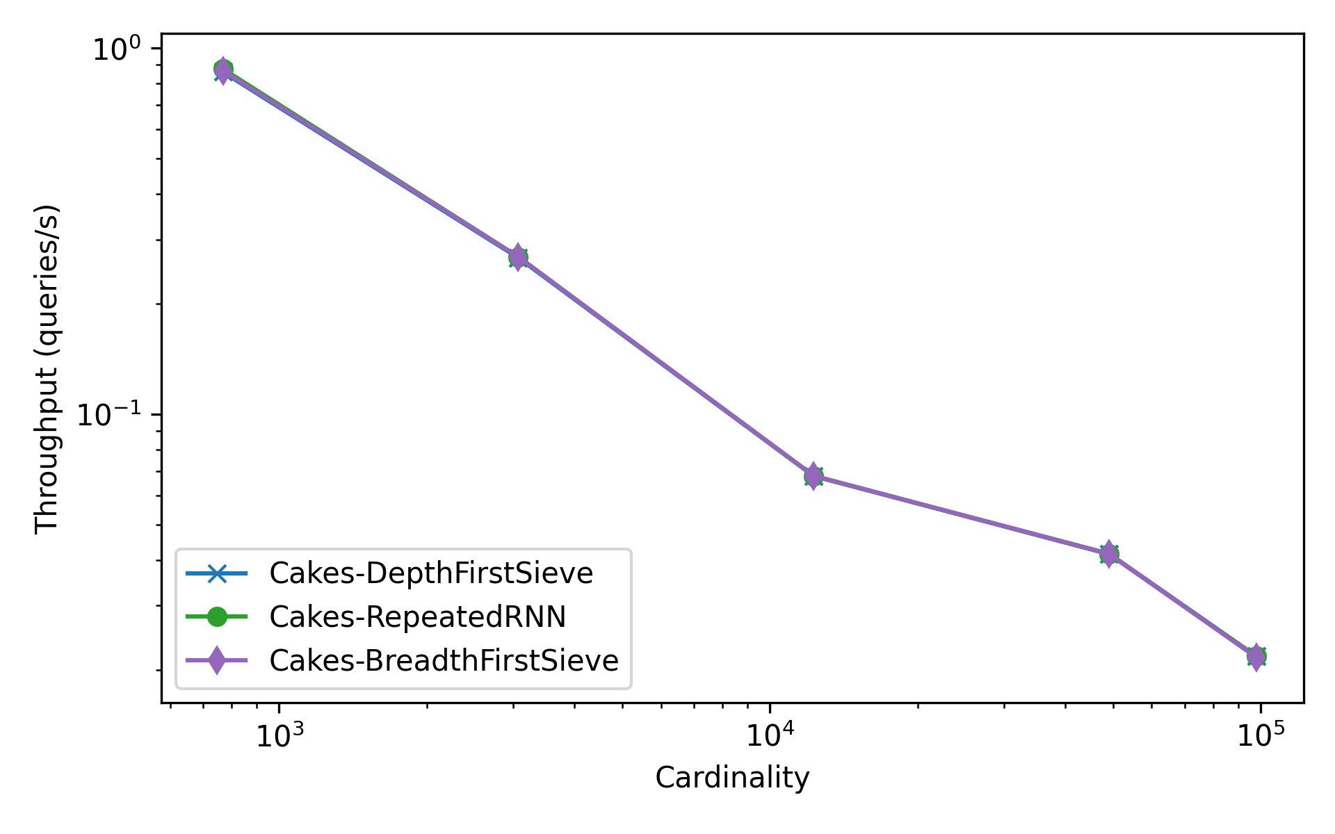
(d) RadioML for $k=10$ at SnR = 10dB.

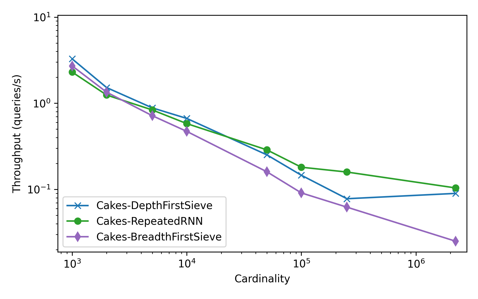
(e) Silva for $k=10$.

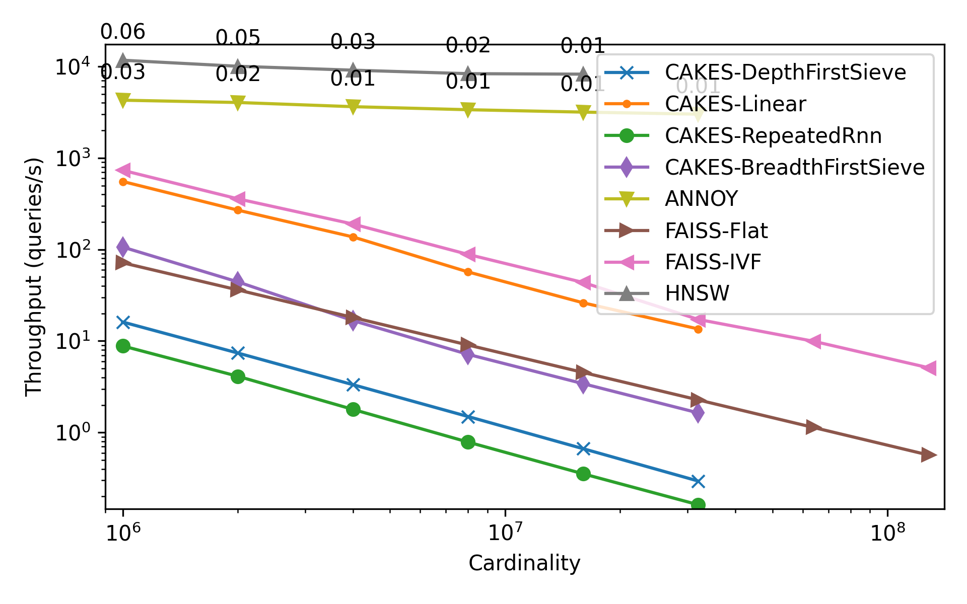
(f) A random dataset for $k=10$.

Figure 5: Throughput across six datasets, including a randomly-generated dataset. In each plot, the horizontal axis represents increasing cardinality of the dataset, while the vertical axis represents the throughput in queries per second (higher is better). Note that for RadioML, all three algorithms performed nearly identically, so distinct lines are not visible. For some algorithms, we were not able to take measurements for each cardinality because the index-building required more RAM than was available (i.e. more then 512GB).

Table 2: QPS (queries per second) and Recall vs naive linear search on the Fashion-Mnist, Glove-25, Sift and Random datasets. A recall value of $1.000*$ denotes imperfect recall that rounds to 1.000.

	Multiplier	hnsw		annoy		faiss-ivf		cakes
		QPS	Recall	QPS	Recall	QPS	Recall	QPS	Recall
Fashion-Mnist	1	1.33 $\times 10^{4}$	0.954	2.19 $\times 10^{3}$	0.950	2.01 $\times 10^{3}$	1.000*	2.17 $\times 10^{3}$	1.000
	2	1.38 $\times 10^{4}$	0.803	2.12 $\times 10^{3}$	0.927	9.39 $\times 10^{2}$	1.000*	1.14 $\times 10^{3}$	1.000
	4	1.66 $\times 10^{4}$	0.681	2.04 $\times 10^{3}$	0.898	4.61 $\times 10^{2}$	0.997	9.82 $\times 10^{2}$	1.000
	8	1.68 $\times 10^{4}$	0.525	1.93 $\times 10^{3}$	0.857	2.26 $\times 10^{2}$	0.995	1.18 $\times 10^{3}$	1.000
	16	1.87 $\times 10^{4}$	0.494	1.84 $\times 10^{3}$	0.862	1.17 $\times 10^{2}$	0.991	1.20 $\times 10^{3}$	1.000
	32	1.56 $\times 10^{4}$	0.542	1.85 $\times 10^{3}$	0.775	5.91 $\times 10^{1}$	0.985	1.16 $\times 10^{3}$	1.000
	64	1.50 $\times 10^{4}$	0.378	1.78 $\times 10^{3}$	0.677	2.61 $\times 10^{1}$	0.968	1.10 $\times 10^{3}$	1.000
	128	1.49 $\times 10^{4}$	0.357	1.66 $\times 10^{3}$	0.538	1.33 $\times 10^{1}$	0.964	1.04 $\times 10^{3}$	1.000
	256	–	–	1.60 $\times 10^{3}$	0.592	6.65 $\times 10^{0}$	0.962	1.06 $\times 10^{3}$	1.000
	512	–	–	1.83 $\times 10^{3}$	0.581	3.56 $\times 10^{0}$	0.949	1.04 $\times 10^{3}$	1.000
Glove-25	1	2.28 $\times 10^{4}$	0.801	2.83 $\times 10^{3}$	0.835	2.38 $\times 10^{3}$	1.000*	7.22 $\times 10^{2}$	1.000*
	2	2.38 $\times 10^{4}$	0.607	2.70 $\times 10^{3}$	0.832	1.19 $\times 10^{3}$	1.000*	5.75 $\times 10^{2}$	1.000*
	4	2.50 $\times 10^{4}$	0.443	2.61 $\times 10^{3}$	0.839	6.19 $\times 10^{2}$	1.000*	6.25 $\times 10^{2}$	1.000*
	8	2.78 $\times 10^{4}$	0.294	2.51 $\times 10^{3}$	0.834	3.03 $\times 10^{2}$	1.000*	5.93 $\times 10^{2}$	1.000*
	16	3.11 $\times 10^{4}$	0.213	2.23 $\times 10^{3}$	0.885	1.51 $\times 10^{2}$	1.000*	5.49 $\times 10^{2}$	1.000*
	32	3.24 $\times 10^{4}$	0.178	2.01 $\times 10^{3}$	0.764	7.40 $\times 10^{1}$	0.999	4.75 $\times 10^{2}$	1.000*
	64	–	–	1.99 $\times 10^{3}$	0.631	3.77 $\times 10^{1}$	0.997	4.61 $\times 10^{2}$	1.000*
	128	–	–	–	–	1.90 $\times 10^{1}$	0.998	4.41 $\times 10^{2}$	1.000*
	256	–	–	–	–	9.47 $\times 10^{0}$	0.998	4.23 $\times 10^{2}$	1.000*
Sift	1	1.93 $\times 10^{4}$	0.782	3.98 $\times 10^{3}$	0.686	6.98 $\times 10^{2}$	1.000*	5.52 $\times 10^{2}$	1.000
	2	2.03 $\times 10^{4}$	0.552	3.80 $\times 10^{3}$	0.614	3.30 $\times 10^{2}$	1.000*	2.66 $\times 10^{2}$	1.000
	4	2.18 $\times 10^{4}$	0.394	3.69 $\times 10^{3}$	0.637	1.65 $\times 10^{2}$	1.000*	1.43 $\times 10^{2}$	1.000
	8	2.48 $\times 10^{4}$	0.298	3.58 $\times 10^{3}$	0.710	7.72 $\times 10^{1}$	1.000*	7.94 $\times 10^{1}$	1.000
	16	2.68 $\times 10^{4}$	0.210	3.50 $\times 10^{3}$	0.690	3.98 $\times 10^{1}$	1.000*	8.12 $\times 10^{1}$	1.000
	32	2.75 $\times 10^{4}$	0.193	3.44 $\times 10^{3}$	0.639	2.09 $\times 10^{1}$	0.999	7.81 $\times 10^{1}$	1.000
	64	–	–	3.39 $\times 10^{3}$	0.678	8.87 $\times 10^{0}$	0.997	7.43 $\times 10^{1}$	1.000
	128	–	–	3.36 $\times 10^{3}$	0.643	4.78 $\times 10^{0}$	0.993	6.80 $\times 10^{1}$	1.000
Random	1	1.17 $\times 10^{4}$	0.060	4.28 $\times 10^{3}$	0.028	7.34 $\times 10^{2}$	1.000*	5.54 $\times 10^{2}$	1.000
	2	1.01 $\times 10^{4}$	0.048	4.04 $\times 10^{3}$	0.021	3.58 $\times 10^{2}$	1.000*	2.69 $\times 10^{2}$	1.000
	4	9.12 $\times 10^{3}$	0.031	3.64 $\times 10^{3}$	0.014	1.90 $\times 10^{2}$	1.000*	1.37 $\times 10^{2}$	1.000
	8	8.35 $\times 10^{3}$	0.022	3.37 $\times 10^{3}$	0.013	8.84 $\times 10^{1}$	1.000*	5.69 $\times 10^{1}$	1.000
	16	8.25 $\times 10^{3}$	0.008	3.17 $\times 10^{3}$	0.006	4.36 $\times 10^{1}$	1.000*	2.61 $\times 10^{1}$	1.000
	32	–	–	3.01 $\times 10^{3}$	0.007	1.72 $\times 10^{1}$	1.000*	1.35 $\times 10^{1}$	1.000

5 Discussion and Future Work

We have presented CAKES, a set of three algorithms for fast $k$-NN search that are generic over a variety of distance functions. CAKES’s algorithms are exact when the distance function in use is a metric (see definition in 2). Even under Cosine distance, which is not a metric, CAKES’s algorithms exhibit nearly perfect recall (i.e. always greater than $0.9995$).

CAKES’s algorithms are designed to be most effective when the data uphold the manifold hypothesis, or in other words, when the data are constrained to a low-dimensional manifold even when embedded in a high-dimensional space. As a consequence, these algorithms do not perform well on data with random distributions, because of the absence of a manifold structure. In Figure 3, we show the extent to which each of the datasets we tested exhibits a manifold structure, as quantified by the percentiles of LFD. As expected, our results from Figure 5 indicate that CAKES’s algorithms scale sub-linearly with cardinality on datasets with low LFD, and scale linearly on datasets with high LFD.

As seen in Figures 3(f) and 3(c), the LFD of the Random dataset is much higher than that of Sift, even though they have the same cardinality and embedding dimension. This is unsurprising, given that the Random dataset is, by definition, uniformly distributed, while Sift is not. On the Random dataset, CAKES’s algorithms’ speed decreases linearly as the multiplier increases, while with Sift, Depth-First Sieve and Breadth-First Sieve both exhibit nearly constant throughput. While Repeated $\rho$-NN does not exhibit near-constant throughput with Sift, the throughput decreases much more slowly than it does with the Random dataset. Since these two datasets have the same cardinality and embedding dimension, the aforementioned discrepancies show the effect of a manifold structure on algorithm performance. We emphasize that even though CAKES’s algorithms are slower on the Random dataset, their recalls remain perfect at all multipliers.

Figure 5 also shows that HNSW and ANNOY have near constant throughput as the multiplier increases, however, their recall continues to decrease as the multiplier increases. This, coupled with the prohibitively increasing cost (in terms of memory and time) of building the indices for HNSW and ANNOY, makes these algorithms unsuitable for real-world applications in which the dataset cardinalities are growing exponentially. CAKES’s tree is orders of magnitude cheaper to build and CAKES’s algorithms, while a little slower than HNSW and ANNOY, still show near constant scaling with cardinality in addition to having perfect recall.

When written with the same notation as used in Section 2.4.5, we see that the time complexity of Repeated $\rho$-NN is $\mathcal{O}(\tfrac{\mathcal{T}}{d}+\mathcal{L})$, where $\mathcal{T}$ is the time complexity of tree-search and $\mathcal{L}$ is the time complexity of leaf-search. Even though Repeated $\rho$-NN has the lowest time complexity (compare to $\mathcal{O}(\mathcal{T}\log{(\mathcal{T}+\mathcal{L})}+\mathcal{L}\log{(\mathcal{T}+\mathcal{L})})$ for Breadth-First Sieve and $\mathcal{O}(\mathcal{T}\log{\mathcal{T}}+\mathcal{L}\log{k})$ for Depth-First Sieve) of the three CAKES algorithms, it is not always the fastest algorithm empirically. We believe that some of this discrepancy can be explained by the fact that if Repeated $\rho$-NN significantly “overshoots” the correct radius for $k$ hits ($\rho_{k}$) during tree-search, leaf-search will require looking at more points, rendering the true scaling factor higher than that in 6. This overshot can occur when the LFDs of clusters near the query are not concentrated around their expectation. For example, if most clusters near the query have very low LFD except for one anomaly with very high LFD, the harmonic mean LFD $\mu$ can still be low, so the factor of radial increase 5 may be much larger than necessary for guaranteeing $k$ hits. This suggests that rather than use the reciprocal of the harmonic mean LFD in 5, we may actually want a mean which is more sensitive to high outliers, such as the geometric mean. We leave it as an avenue for future work to characterize when Repeated $\rho$-NN significantly “overshoots” $\rho_{k}$ and to improve upon the factor of radial increase in 5 so that this overshooting occurs less frequently and with less severity.

As the previous paragraph suggests, the fastest CAKES algorithm varies by dataset. For example, on Glove-25, Repeated $\rho$-NN exhibits the highest throughput of any CAKES algorithm, despite having the lowest throughput of the three on Sift and Fashion-Mnist. On Silva, Repeated $\rho$-NN is comparable to the other CAKES algorithms at low multipliers, but becomes the fastest at the higher multipliers. When we view these results in light of the LFD plots in Figure 3, we realize that Repeated $\rho$-NN appears to be the fastest CAKES algorithm on datasets where a large proportion of the data have a very low LFD, such as Glove-25 and Silva. This trend is unsurprising, given that Repeated $\rho$-NN relies on a low LFD around the query in order to quickly estimate the correct radius for $k$ hits. These findings suggest that Repeated $\rho$-NN is the most “sensitive” to the manifold structure of the dataset. Exploring this sensitivity is a potential avenue for future investigation, as it remains to be determined at what LFD Repeated $\rho$-NN transitions away from being the fastest CAKES algorithm, and whether this transition is sharp.

While the fastest CAKES algorithm varies by dataset, we observe that on all three ANN-benchmark datasets (Fashion-Mnist, Glove-25, and Sift), Depth-First Sieve and Breadth-First Sieve show nearly constant throughput as the cardinality increases. This observation warrants further investigation, but it is especially promising given that Depth-First Sieve and Breadth-First Sieve consistently outperform linear search for high cardinalities. Finally, we emphasize that the variation in performance of our algorithms across different datasets and cardinalities supports our use of an auto-tuning function (as discussed in Section 2.5) to select the best algorithm for a given dataset. Future work is needed to better characterize those datasets for which each algorithm performs best, but our results suggest that a more sophisticated auto-tuning function could be developed to select the fastest algorithm based on the properties of the dataset.

We also stress that CAKES’s algorithms are designed to work well for big data, and our results support this claim; we observe that while linear search can outperform CAKES on datasets with small cardinality, CAKES always overtakes linear search at a large enough cardinality for each of the ANN-benchmarks’ datasets we tested. Moreover, we observe that CAKES’s algorithms outperform linear search at a lower cardinality when the dataset has a lower LFD. For example, Sift has much higher LFD than Fashion-Mnist and Glove-25, and we observe that CAKES overtakes linear search at a cardinality of $10^{7}$ for Sift, as opposed to about $10^{5}$ and $10^{6}$ for Fashion-Mnist and Glove-25, respectively. For the Random dataset, which has the highest LFD, CAKES’s algorithms never outperform linear search. These observations support our claim that CAKES performs well on datasets that arise from constrained generating phenomena, even as the cardinalities of these datasets grow exponentially.

The questions raised by this study suggest several additional avenues for future work. A comparison across more datasets is in order, as is further analysis with other distance functions that existing methods, such as FAISS, HNSW and ANNOY, do not support, such as Wasserstein distance [37] for probability distributions (particularly for high dimensional distributions), and Tanimoto distance [38] for comparing molecular structures by their maximal common subgraphs. Incorporating these or other distance functions in CAKES requires only that a Rust implementation of the distance function be provided.

We also plan to investigate hierarchical data compression by representing differences at each level of the binary tree, particularly for string or genomic data, where all differences are discrete. Such an encoding would allow us to store the data in a compressed format, and to perform search on the compressed data without decompressing it. This would allow us to perform fast search on datasets that are too large to fit in memory. An exploration of compression and compressed search is an avenue for future work.

Another avenue for future work is to explore the use of CAKES in a streaming environment. This would require the ability to perform “online” updates to the tree as points are added to or deleted from the dataset. Such online updates would take advantage of the fast search algorithms provided by CAKES. CAKES can also be used to extend anomaly detection in CHAODA [32]. We could add to CHAODA’s ensemble of graph-based anomaly detection methods by using the distribution of distances among the $k$ nearest neighbors of cluster centers.

CLAM and CAKES are implemented in Rust and the source code is available under an MIT license at https://github.com/URI-ABD/clam.

6 Supplementary Results

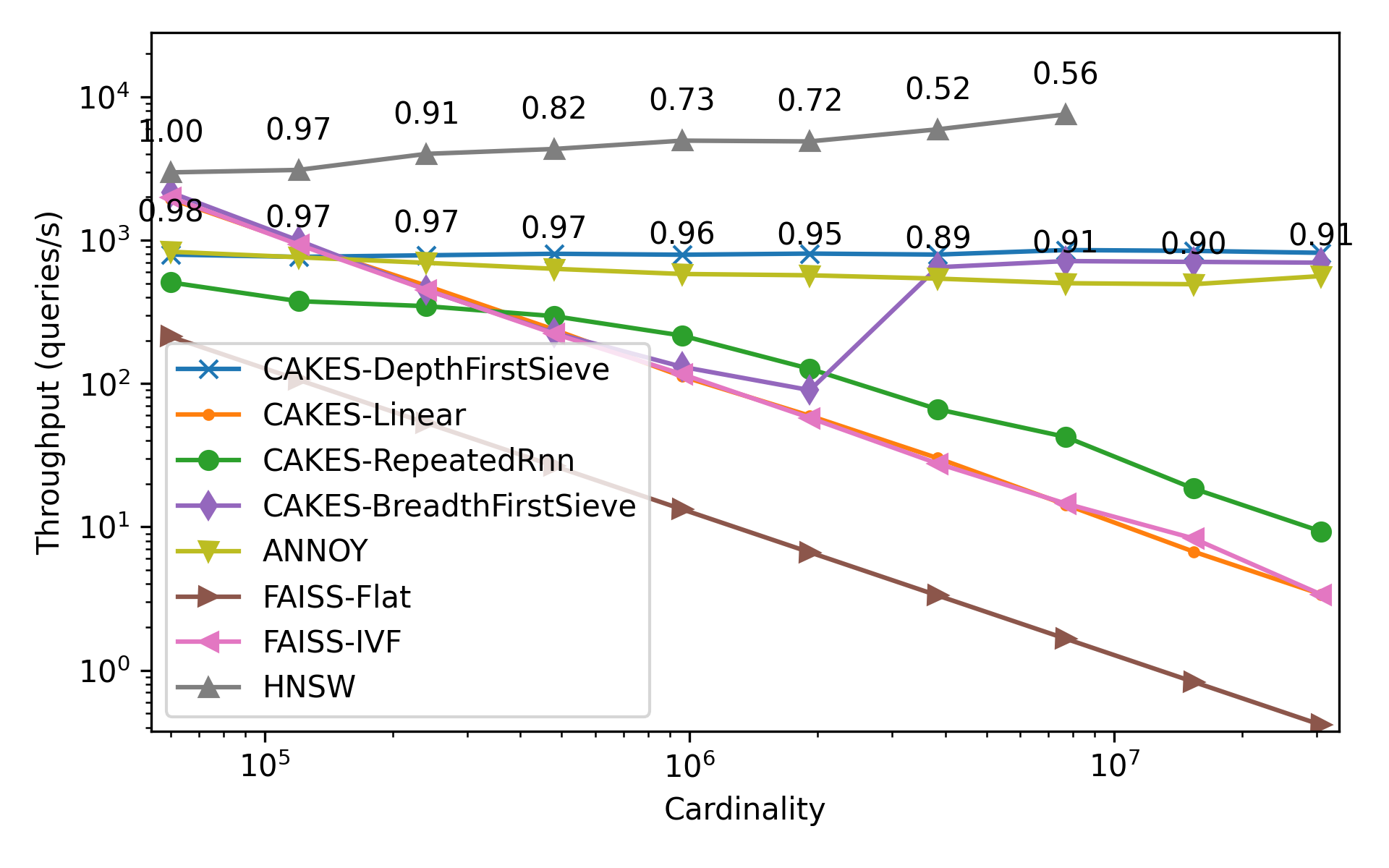
Figure 6: Scaling behavior of algorithms on fashion-mnist with $k=100$.

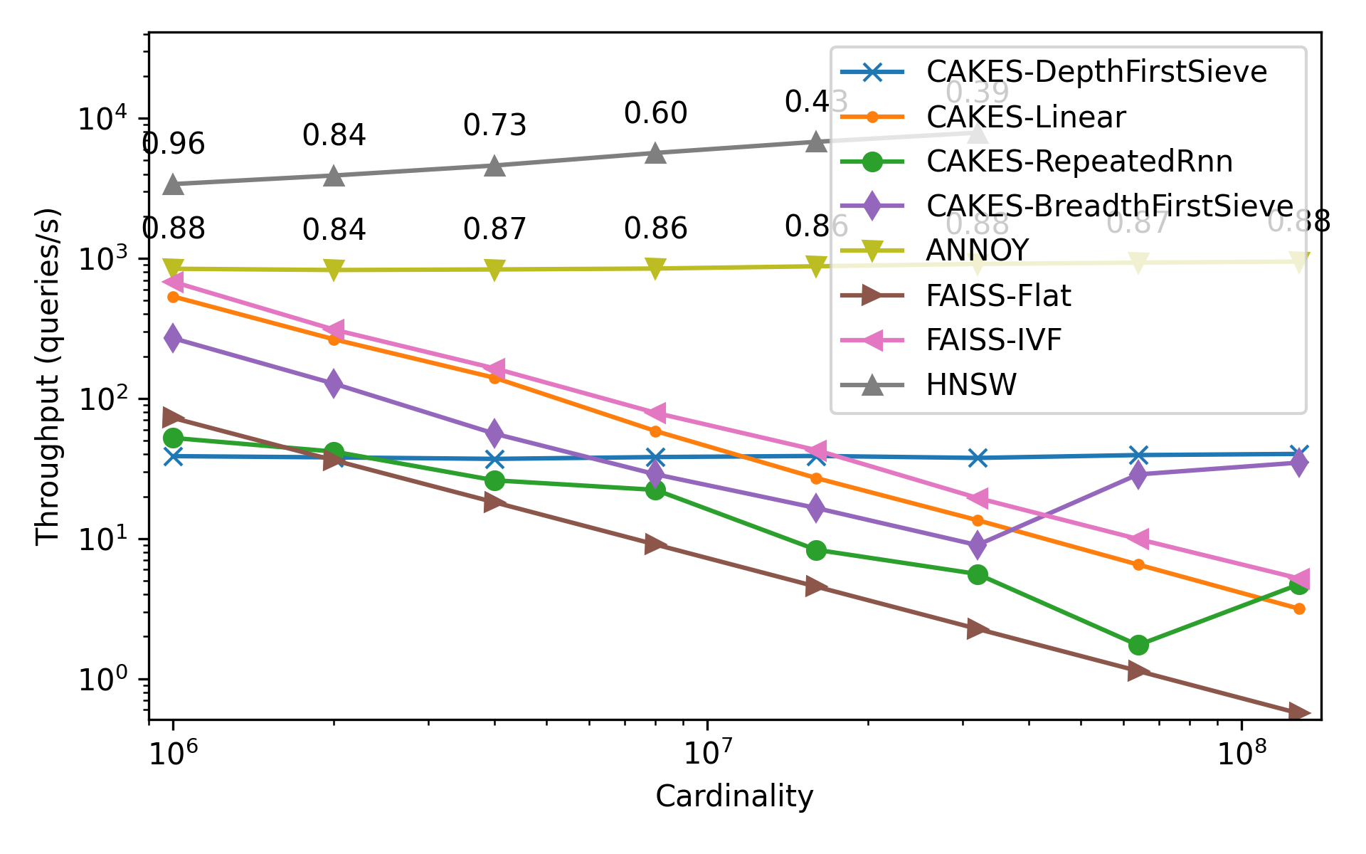
Figure 7: Scaling behavior of algorithms on sift with $k=100$.

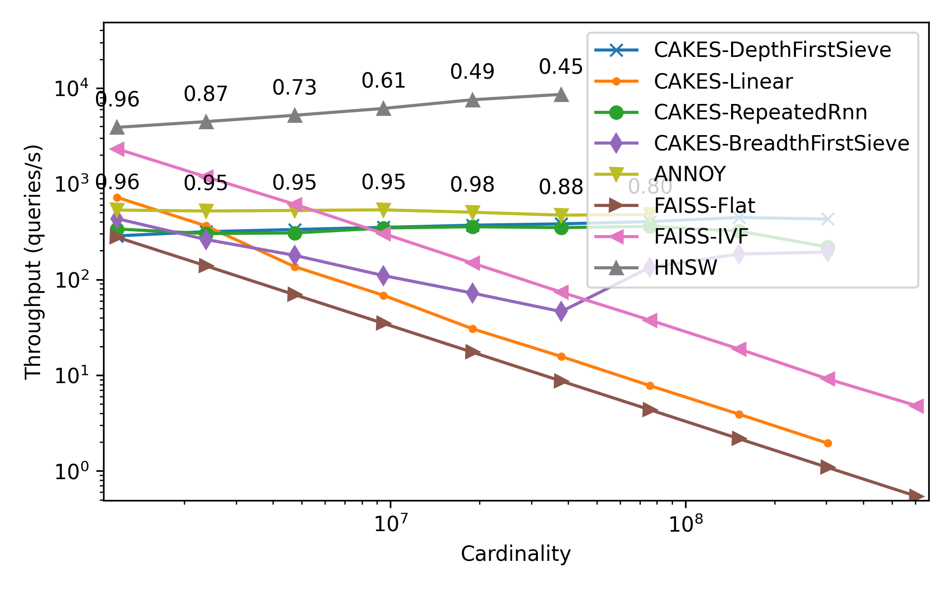
Figure 8: Scaling behavior of algorithms on glove-25 with $k=100$.

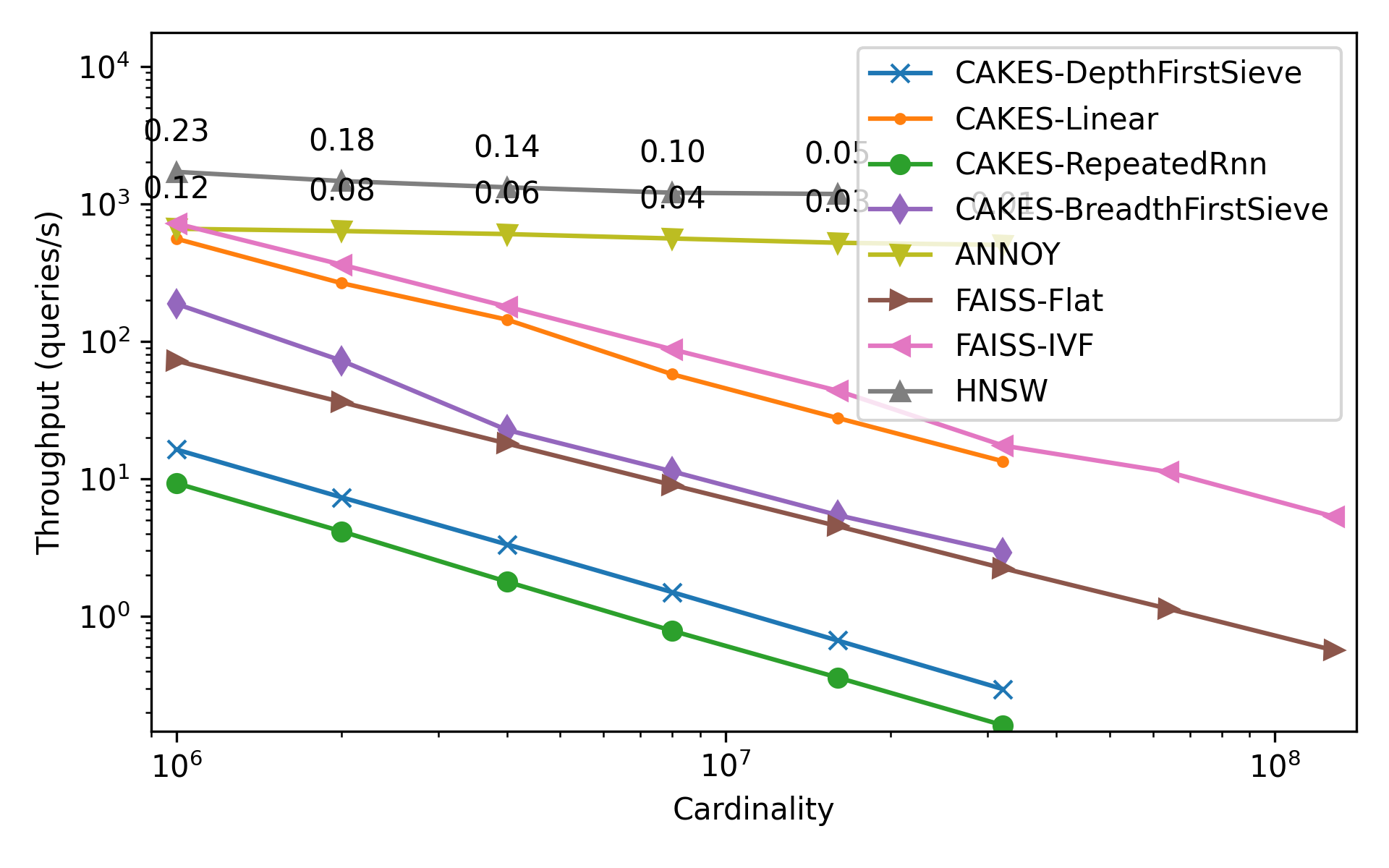
Figure 9: Scaling behavior of algorithms on random with $k=100$.

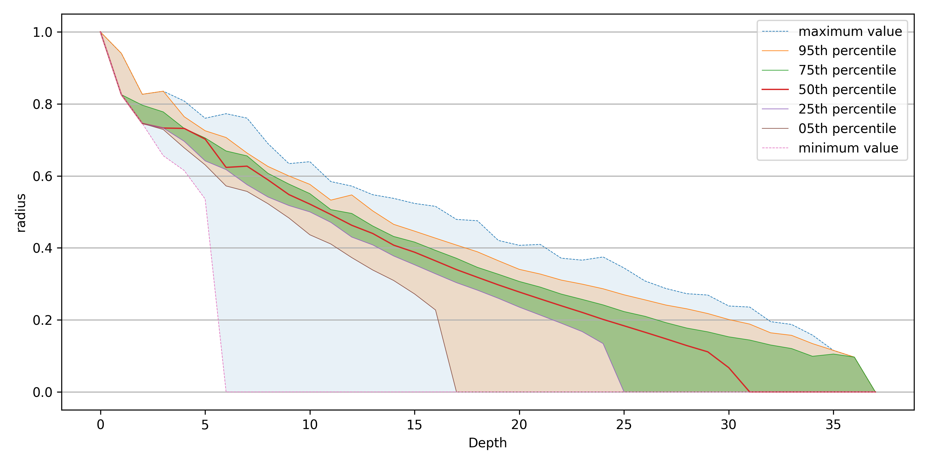
(a) Fashion-mnist

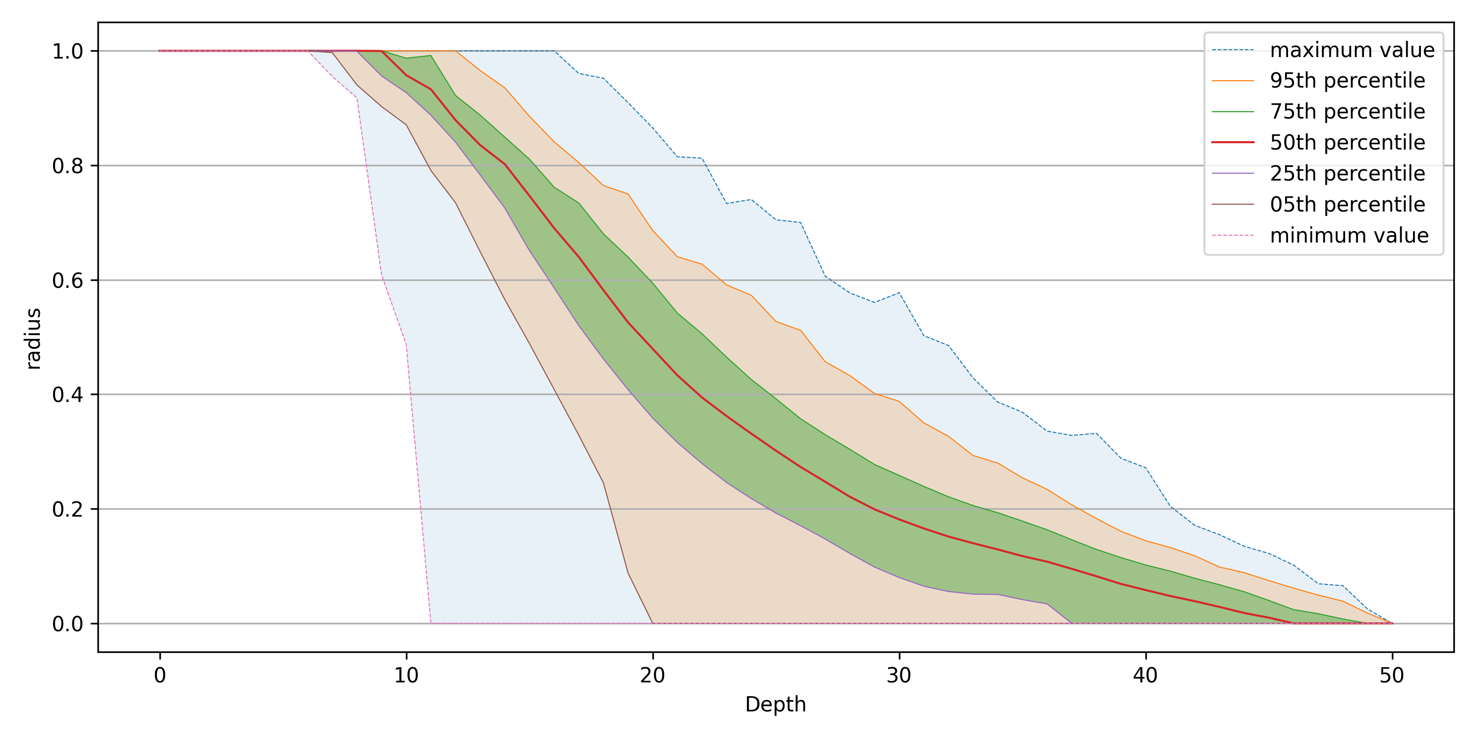
(b) Glove-25

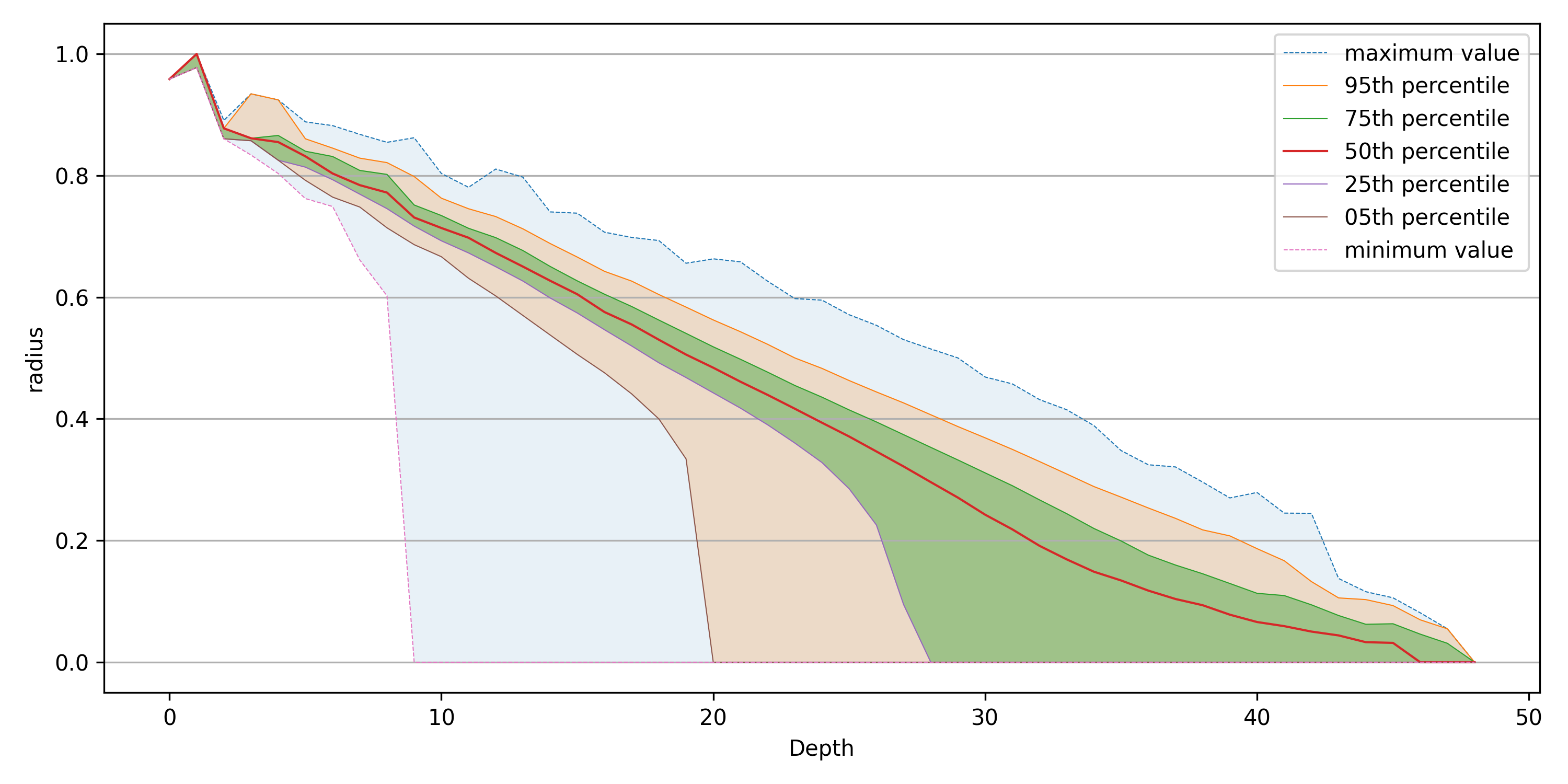
(c) Sift

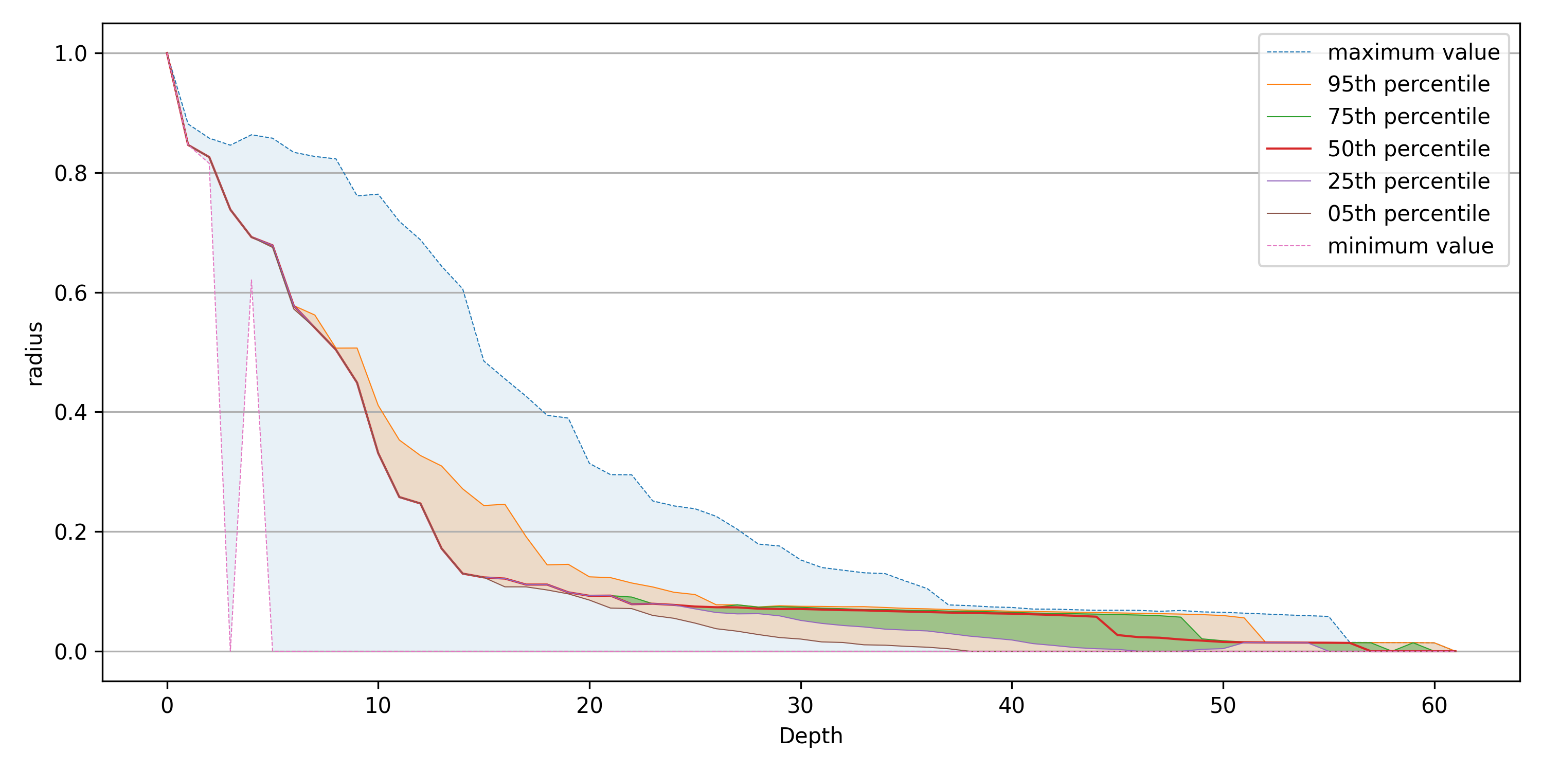
(d) RadioML

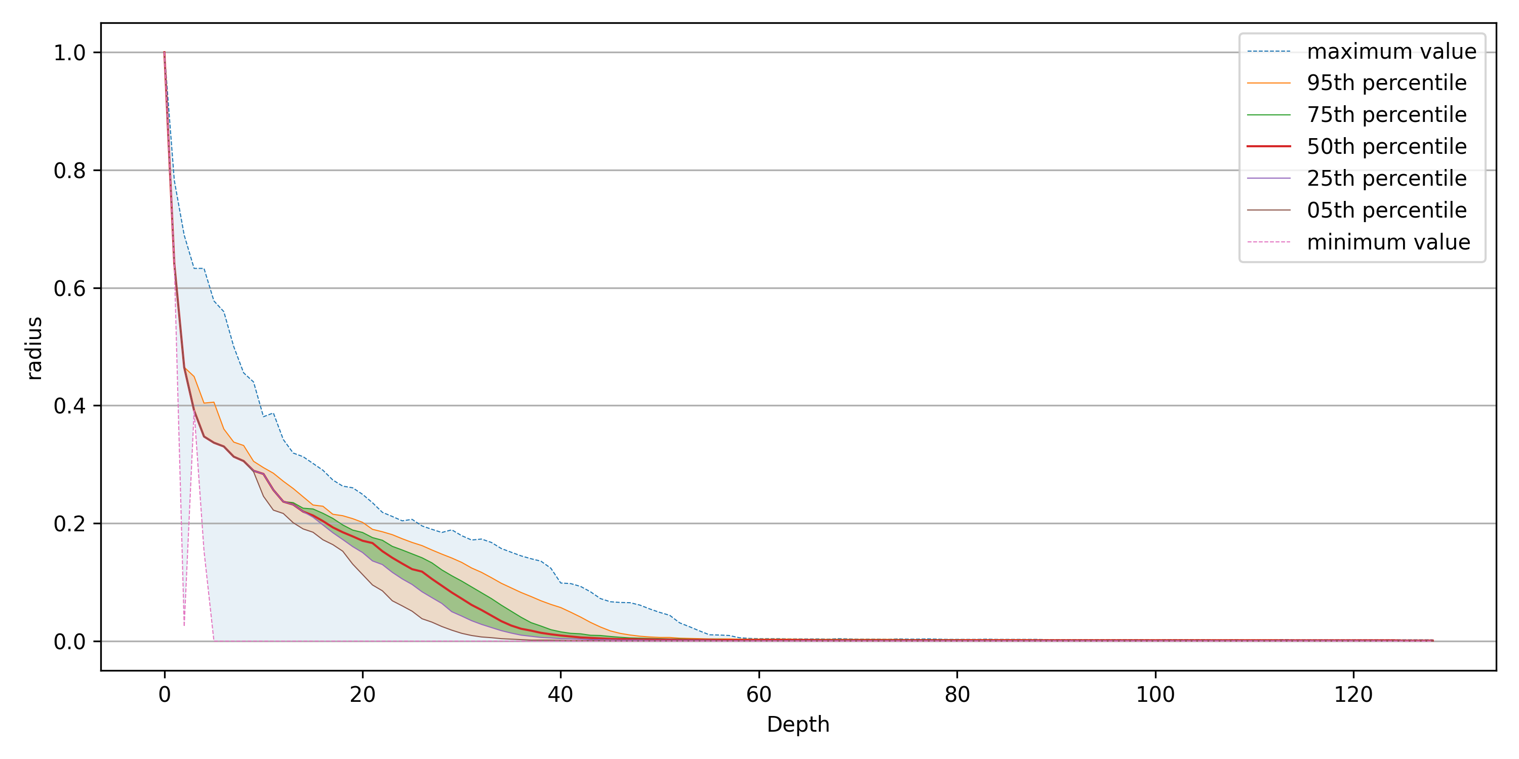
(e) Silva 18S

(f) A random dataset

Figure 10: Radius vs. cluster depth across six datasets, grouped by decile of radius and weighted by the cardinalities of the clusters. The last dataset is randomly generated.

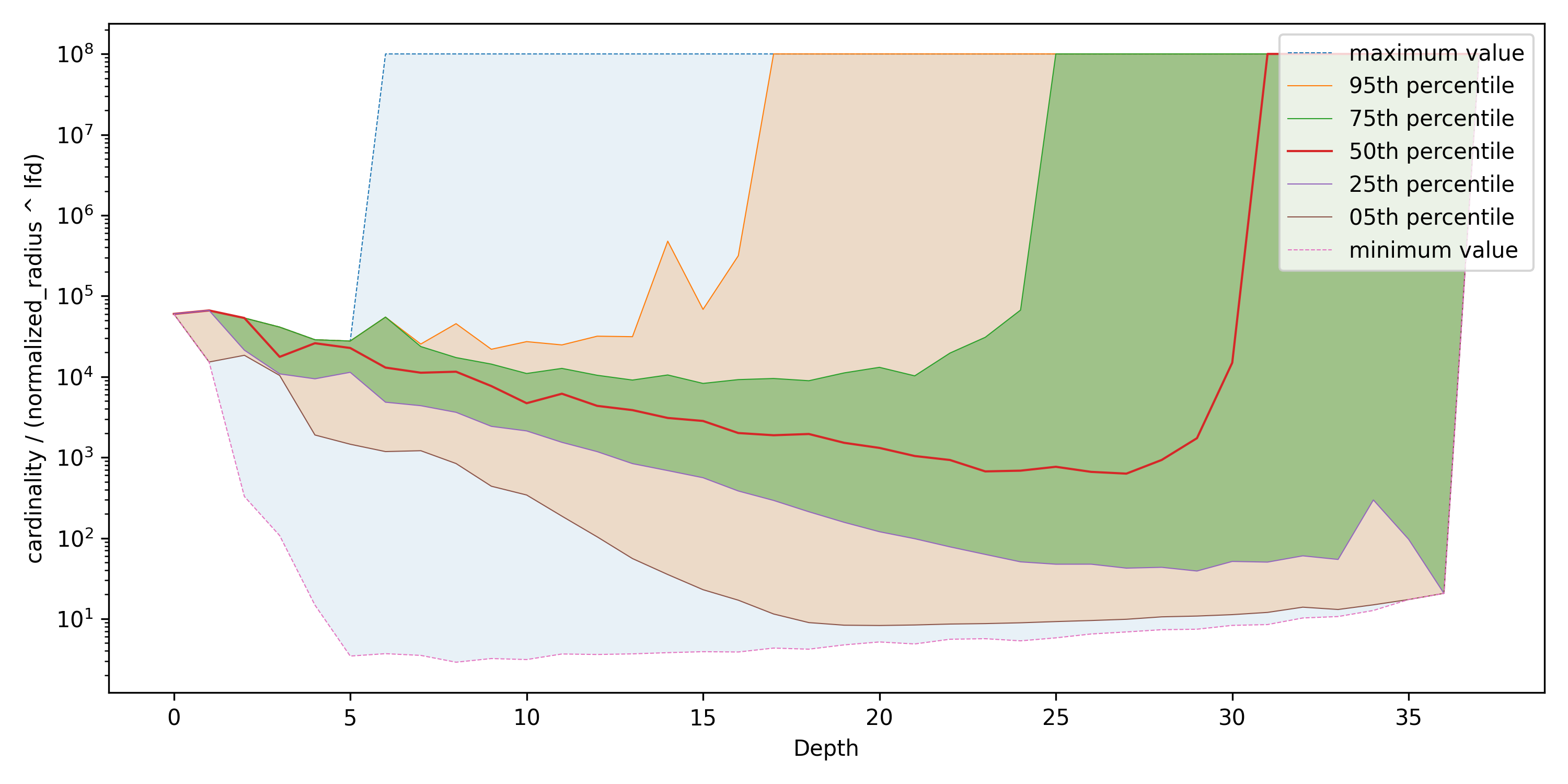
(a) Fashion-mnist

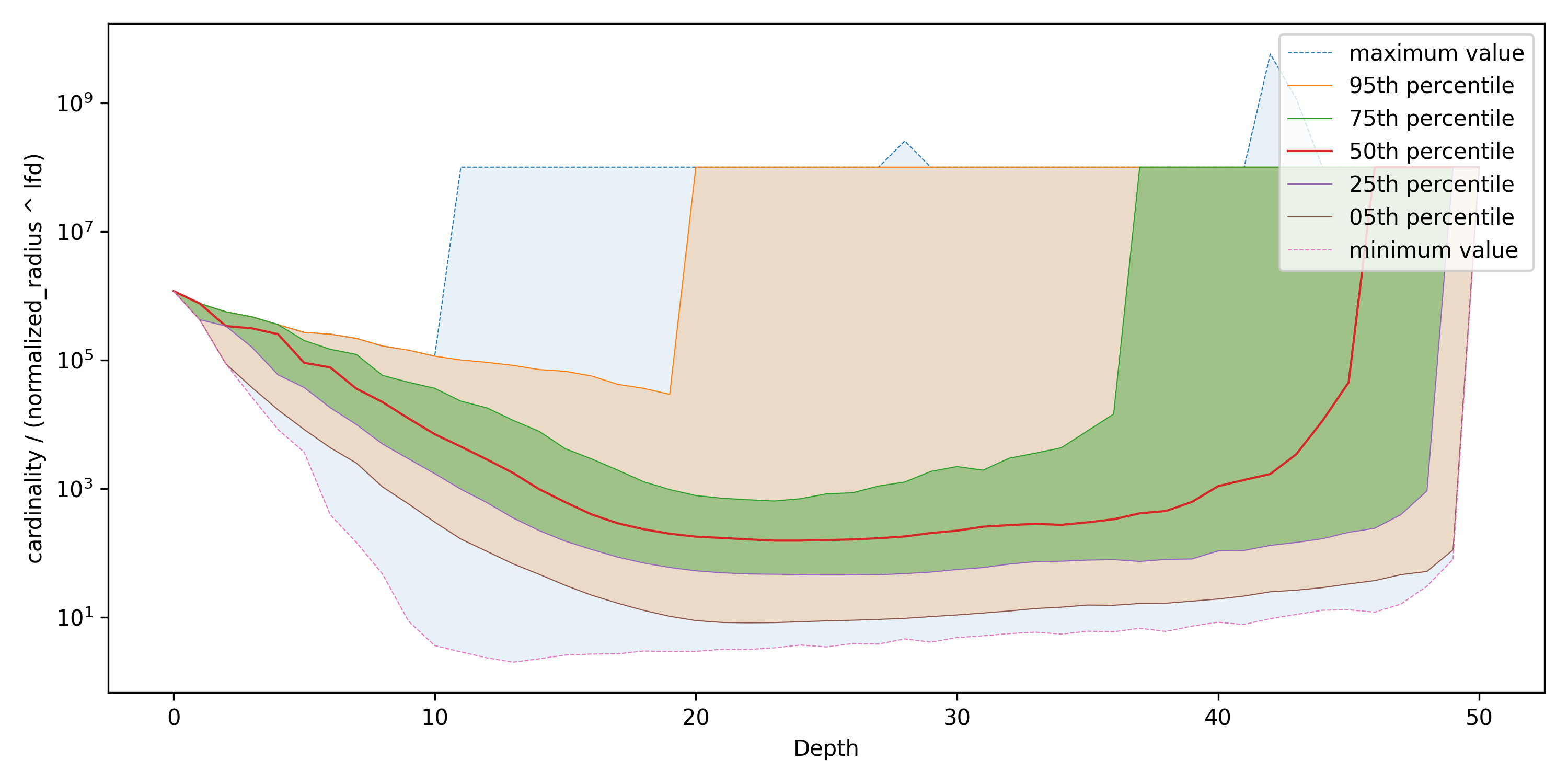
(b) Glove-25

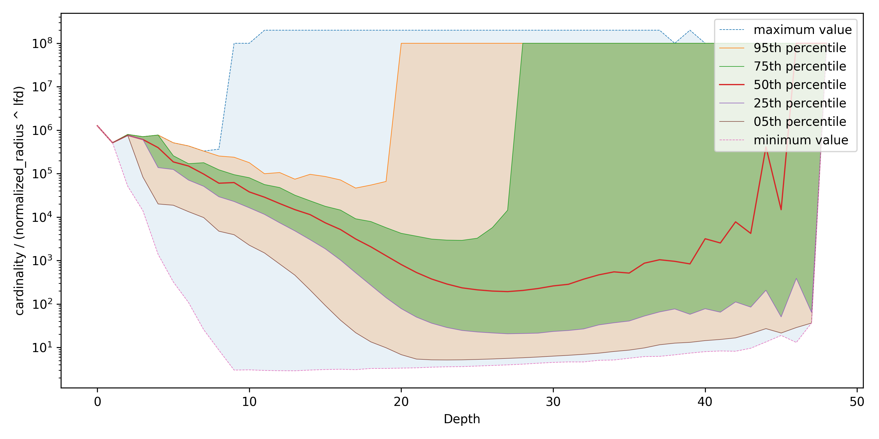
(c) Sift

(d) RadioML

(e) Silva 18S

(f) A random dataset

Figure 11: Fractal Density vs. cluster depth across six datasets, grouped by decile of fractal density and weighted by the cardinalities of the clusters. The last dataset is randomly generated. Fractal Density is defined as $\frac{cardinality}{radius^{LFD}}$

References

- [1] S. D. Kahn, “On the future of genomic data,” Science, vol. 331, no. 6018, pp. 728–729, 2011.
- [2] T. B. Brown, B. Mann, N. Ryder, M. Subbiah, J. Kaplan, P. Dhariwal, A. Neelakantan, P. Shyam, G. Sastry, A. Askell, S. Agarwal, A. Herbert-Voss, G. Krueger, T. Henighan, R. Child, A. Ramesh, D. M. Ziegler, J. Wu, C. Winter, C. Hesse, M. Chen, E. Sigler, M. Litwin, S. Gray, B. Chess, J. Clark, C. Berner, S. McCandlish, A. Radford, I. Sutskever, and D. Amodei, “Language Models are Few-Shot Learners,” arXiv e-prints, p. arXiv:2005.14165, May 2020.
- [3] OpenAI, “Gpt-4 technical report,” ArXiv, vol. abs/2303.08774, 2023.
- [4] H. Touvron, L. Martin, K. R. Stone, P. Albert, A. Almahairi, Y. Babaei, N. Bashlykov, S. Batra, P. Bhargava, S. Bhosale, D. M. Bikel, L. Blecher, C. C. Ferrer, M. Chen, G. Cucurull, D. Esiobu, J. Fernandes, J. Fu, W. Fu, B. Fuller, C. Gao, V. Goswami, N. Goyal, A. S. Hartshorn, S. Hosseini, R. Hou, H. Inan, M. Kardas, V. Kerkez, M. Khabsa, I. M. Kloumann, A. V. Korenev, P. S. Koura, M.-A. Lachaux, T. Lavril, J. Lee, D. Liskovich, Y. Lu, Y. Mao, X. Martinet, T. Mihaylov, P. Mishra, I. Molybog, Y. Nie, A. Poulton, J. Reizenstein, R. Rungta, K. Saladi, A. Schelten, R. Silva, E. M. Smith, R. Subramanian, X. Tan, B. Tang, R. Taylor, A. Williams, J. X. Kuan, P. Xu, Z. Yan, I. Zarov, Y. Zhang, A. Fan, M. Kambadur, S. Narang, A. Rodriguez, R. Stojnic, S. Edunov, and T. Scialom, “Llama 2: Open foundation and fine-tuned chat models,” ArXiv, vol. abs/2307.09288, 2023. [Online]. Available: https://api.semanticscholar.org/CorpusID:259950998
- [5] A. Radford, J. W. Kim, C. Hallacy, A. Ramesh, G. Goh, S. Agarwal, G. Sastry, A. Askell, P. Mishkin, J. Clark et al., “Learning transferable visual models from natural language supervision,” in International conference on machine learning. PMLR, 2021, pp. 8748–8763.
- [6] A. Dosovitskiy, L. Beyer, A. Kolesnikov, D. Weissenborn, X. Zhai, T. Unterthiner, M. Dehghani, M. Minderer, G. Heigold, S. Gelly et al., “An image is worth 16x16 words: Transformers for image recognition at scale,” arXiv preprint arXiv:2010.11929, 2020.
- [7] T. Z. DeSantis, P. Hugenholtz, N. Larsen, M. Rojas, E. L. Brodie, K. Keller, T. Huber, D. Dalevi, P. Hu, and G. L. Andersen, “Greengenes, a chimera-checked 16s rrna gene database and workbench compatible with arb,” Appl. Environ. Microbiol., vol. 72, no. 7, pp. 5069–5072, 2006.
- [8] C. Quast, E. Pruesse, P. Yilmaz, J. Gerken, T. Schweer, P. Yarza, J. Peplies, and F. O. Glöckner, “The SILVA ribosomal RNA gene database project: improved data processing and web-based tools,” Nucleic Acids Research, vol. 41, no. D1, pp. D590–D596, 11 2012.
- [9] T. J. O’Shea, T. Roy, and T. C. Clancy, “Over-the-air deep learning based radio signal classification,” IEEE Journal of Selected Topics in Signal Processing, vol. 12, no. 1, pp. 168–179, 2018.
- [10] E. Bernhardsson, “Annoy,” https://github.com/spotify/annoy, 2015.
- [11] S. Suyanto, P. E. Yunanto, T. Wahyuningrum, and S. Khomsah, “A multi-voter multi-commission nearest neighbor classifier,” Journal of King Saud University - Computer and Information Sciences, vol. 34, no. 8, Part B, pp. 6292–6302, 2022.
- [12] Y. Malkov and D. A. Yashunin, “Efficient and robust approximate nearest neighbor search using hierarchical navigable small world graphs,” IEEE Transactions on Pattern Analysis and Machine Intelligence, vol. 42, pp. 824–836, 2016. [Online]. Available: https://api.semanticscholar.org/CorpusID:8915893
- [13] J. Johnson, M. Douze, and H. Jégou, “Billion-scale similarity search with GPUs,” IEEE Transactions on Big Data, vol. 7, no. 3, pp. 535–547, 2019.
- [14] M. Aumüller, E. Bernhardsson, and A. Faithfull, “Ann-benchmarks: A benchmarking tool for approximate nearest neighbor algorithms,” Information Systems, vol. 87, p. 101374, 2020.
- [15] E. Fix and J. L. Hodges Jr, “Discriminatory analysis-nonparametric discrimination: Small sample performance,” California Univ Berkeley, Tech. Rep., 1952.
- [16] T. M. Cover, P. Hart et al., “Nearest neighbor pattern classification,” IEEE transactions on information theory, vol. 13, no. 1, pp. 21–27, 1967.
- [17] J. Zhang, T. Wang, W. W. Ng, and W. Pedrycz, “Ensembling perturbation-based oversamplers for imbalanced datasets,” Neurocomput., vol. 479, no. C, p. 1–11, mar 2022. [Online]. Available: https://doi.org/10.1016/j.neucom.2022.01.049
- [18] L.-Y. Hu, M.-W. Huang, S.-W. Ke, and C.-F. Tsai, “The distance function effect on k-nearest neighbor classification for medical datasets,” SpringerPlus, vol. 5, no. 1, pp. 1–9, 2016.
- [19] I. Budowski-Tal, Y. Nov, and R. Kolodny, “Fragbag, an accurate representation of protein structure, retrieves structural neighbors from the entire pdb quickly and accurately,” Proceedings of the National Academy of Sciences, vol. 107, no. 8, pp. 3481–3486, 2010.
- [20] E. Ukkonen, “Algorithms for approximate string matching,” Information and control, vol. 64, no. 1-3, pp. 100–118, 1985.
- [21] P. Zhang, “Privacy preserving similarity search for online advertising,” 2020.
- [22] N. Ishaq, G. Student, and N. M. Daniels, “Clustered hierarchical entropy-scaling search of astronomical and biological data,” in 2019 IEEE International Conference on Big Data (Big Data). IEEE, 2019, pp. 780–789.
- [23] Y. A. Malkov and D. A. Yashunin, “Efficient and robust approximate nearest neighbor search using hierarchical navigable small world graphs,” CoRR, vol. abs/1603.09320, 2016. [Online]. Available: http://arxiv.org/abs/1603.09320
- [24] V. I. Levenshtein et al., “Binary codes capable of correcting deletions, insertions, and reversals,” in Soviet physics doklady, vol. 10, no. 8. Soviet Union, 1966, pp. 707–710.
- [25] O. Gold and M. Sharir, “Dynamic time warping and geometric edit distance: Breaking the quadratic barrier,” ACM Transactions on Algorithms (TALG), vol. 14, no. 4, pp. 1–17, 2018.
- [26] “Faiss-ivf,” https://github.com/facebookresearch/faiss/wiki/Faiss-indexes, 2016.
- [27] Y. W. Yu, N. Daniels, D. C. Danko, and B. Berger, “Entropy-scaling search of massive biological data,” Cell Systems, vol. 1, no. 2, pp. 130–140, 2015.
- [28] J. M. Kleinberg, “Navigation in a small world,” Nature, vol. 406, no. 6798, pp. 845–845, 2000.
- [29] M. Boguna, D. Krioukov, and K. C. Claffy, “Navigability of complex networks,” Nature Physics, vol. 5, no. 1, pp. 74–80, 2009.
- [30] R. Sacks-Davis, A. Kent, and K. Ramamohanarao, “Multikey access methods based on superimposed coding techniques,” ACM Transactions on Database Systems (TODS), vol. 12, no. 4, pp. 655–696, 1987.
- [31] A. Kent, R. Sacks-Davis, and K. Ramamohanarao, “A signature file scheme based on multiple organizations for indexing very large text databases,” Journal of the american society for information science, vol. 41, no. 7, pp. 508–534, 1990.
- [32] N. Ishaq, T. J. Howard, and N. M. Daniels, “Clustered hierarchical anomaly and outlier detection algorithms,” in 2021 IEEE International Conference on Big Data (Big Data). IEEE, 2021, pp. 5163–5174.
- [33] M. Müller, “Dynamic time warping,” Information retrieval for music and motion, pp. 69–84, 2007.
- [34] C. Fefferman, S. Mitter, and H. Narayanan, “Testing the manifold hypothesis,” Journal of the American Mathematical Society, vol. 29, no. 4, pp. 983–1049, 2016.
- [35] C. A. Hoare, “Algorithm 65: find,” Communications of the ACM, vol. 4, no. 7, pp. 321–322, 1961.
- [36] M. Aumüller, E. Bernhardsson, and A. Faithfull, “Ann-benchmarks: A benchmarking tool for approximate nearest neighbor algorithms,” Inf. Syst., vol. 87, 2018.
- [37] S. Vallender, “Calculation of the wasserstein distance between probability distributions on the line,” Theory of Probability & Its Applications, vol. 18, no. 4, pp. 784–786, 1974.
- [38] D. Bajusz, A. Rácz, and K. Héberger, “Why is tanimoto index an appropriate choice for fingerprint-based similarity calculations?” Journal of cheminformatics, vol. 7, no. 1, pp. 1–13, 2015.