Extended Josephson junction qubit system

Abstract

Circuit quantum electrodynamics (QED) has emerged as a promising platform for implementing quantum computation and simulation. Typically, junctions in these systems are of a sufficiently small size, such that only the lowest plasma oscillation is relevant. The interplay between the Josephson effect and charging energy renders this mode nonlinear, forming the basis of a qubit. In this work, we introduce a novel QED architecture based on extended Josephson Junctions (JJs), which possess a non-negligible spatial extent. We present a comprehensive microscopic analysis and demonstrate that each extended junction can host multiple nonlinear plasmon modes, effectively functioning as a multi-qubit interacting system, in contrast to conventional JJs. Furthermore, the phase modes exhibit distinct spatial profiles, enabling individual addressing through frequency-momentum selective coupling to photons. Our platform has potential applications in quantum computation, specifically in implementing single- and two-qubit gates within a single junction. We also investigate a setup comprising several driven extended junctions interacting via a multimode electromagnetic waveguide. This configuration serves as a powerful platform for simulating the generalized Bose-Hubbard model, as the photon-mediated coupling between junctions can create a lattice in both real and synthetic dimensions. This allows for the exploration of novel quantum phenomena, such as topological phases of interacting many-body systems.

I Introduction

Josephson qubits, characterized by strong nonlinearity and low dissipation, serve as promising building blocks for quantum computers (Devoret and Schoelkopf, 2013) and quantum simulators of complex many-body systems (Houck et al., 2012; Carusotto et al., 2020). Fundamentally, these qubits encode quantum information in the form of plasma oscillations occurring between two superconducting elements. Although this is an intrinsically collective phenomenon within a many-electron system, each junction typically operates within a regime that hosts only a single qubit (Kjaergaard et al., 2020). Various methods exist for interfacing these qubits, such as coupling to a waveguide or an electromagnetic resonator (Majer et al., 2007). When the junction size is sufficiently small, it can be treated as a lumped element, and its interaction with the electromagnetic field is considered as an oscillating point-like dipole (Blais et al., 2004, 2021).

However, more complex scenarios involving multiple junctions or a multimode resonator present a challenging theoretical problem. These are often addressed phenomenologically using the so-called black-box quantization or energy-participation ratio approaches (Nigg et al., 2012; Minev et al., 2021). These methods are only valid in the weak nonlinearity limit, and the regime of strong light-matter interaction is inaccessible. Furthermore, as the number of parameters increases, determining all coefficients within the black-box quantization framework becomes impractical. More generally, the dipole picture loses its validity when the junction size becomes comparable to or larger than the Josephson penetration length ($\lambda_{J}$), which characterizes the stiffness of phase fluctuations in junctions. As a result, the extended quasi-1D junctions can host multiple plasmon modes with the discrete spectrum given by:

$$\omega_{m}=\omega_{{\rm{pl}}}\sqrt{1+\left(\frac{\lambda_{J}}{L}\pi m\right)^{2},}$$ (1)

where $\omega_{{\rm{pl}}}$ is the fundamental plasma frequency. We note that in circuit-QED architecture, conventional qubits correspond to the $m=0$ plasmonic mode as described in Eq. (1). This mode prevails in small junctions where $L$ is significantly smaller than $\lambda_{J}$. On the other hand, as we approach the opposite limit, the plasmon spectrum undergoes a transformation into a continuous form (Tinkham, 2004; Sboychakov et al., 2008). This is accompanied by a reduction in the non-linearity of these modes, and the full dynamics can be effectively described by the classical sine-Gordon equations. While the investigation of this classical regime has a rich history (Ustinov et al., 1993; Ustinov, 1998; Kemp et al., 2002), given the technological developments in the past several decades, it is interesting to explore the quantum regime of such systems. The intermediate regime, $L\sim\lambda_{J}$, is particularly interesting since one can expect several low-energy plasmon modes to be accessible while the strong nonlinearity is not compromised.

In this work, we investigate the light-matter interaction within extended junctions, taking into consideration the inherent complexity of each junction and its multiple degrees of freedom. From a conceptual point of view, our setup could be considered a “beyond dipole-approximation circuit-QED architecture.” Besides, in contrast to the black-box quantization, we follow a microscopic approach and derive both linear and nonlinear terms of the corresponding Hamiltonian. To this end, we develop a general theoretical framework for the quantum description of extended junctions and their interaction with the electromagnetic field. More precisely, we consider a fully microscopic model of two infinitely thin superconducting layers and their coupling with the resonator, which is depicted in Fig. 1 (a). We also microscopically derive the Kerr and cross-Kerr non-linear interaction terms between different plasmon modes. Effectively, each junction operates as an interacting multi-qubit system, and we put forward a strategy for performing single- and two-qubit gates. Furthermore, the spatial extent of the electronic wavefunction for each plasmon mode in light-matter coupling is leveraged to achieve complete qubit addressability, underscoring its practicality for quantum computing applications.

We note that our approach allows us to not only to derive the black-box quantization result in a bottom-up way but also provides a way to engineer effective Hamiltonians based on the mutual spatial structure of the plasmon and resonator modes. In particular, we extend our analysis to the case of many extended junctions coupled to a single waveguide and demonstrate that such a setup could be used in order to simulate complex many-body interacting Hamiltonians from generalized Bose-Hubbard model to potentially lattice gauge theories. We note that our architecture is distinct from the multi-junction circuit-QED (Fitzpatrick et al., 2017), where the qubits do not interact unless they are coupled via resonator. In contrast, in our proposal, nonlinear plasmon qubits do interact with each other and their coupling can be controlled by driving the system, i.e., a 1D array of them makes a 2D synthetic array with full controllability. Our work is also distinct from the giant atom scheme, where the JJ phase is a single number (Kockum et al., 2014; Wang et al., 2021; Kannan et al., 2020).

This paper is structured as follows. In Sec. II, we introduce classical sine-Gordon Lagrangian and perform quantization of the phase fluctuations ignoring the nonlinearity. The latter is then added perturbatively, inducing Kerr, cross-Kerr, and parametric interaction terms between plasmon modes. This action can be obtained from fully microscopic considerations as we show in Appendix  A. In Sec. III, we derive the coupling of the quantized fluctuations of the junction to the electromagnetic field of a coplanar waveguide. In Sec. IV-V, we propose an architecture for quantum computation and simulation based on an array of extended Josephson junctions coupled to a single waveguide.

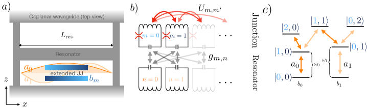
Figure 1: Extended Josephson Junction qubit. (a) An extended Josephson junction is placed in the center of the resonator. Superconducting phase fluctuations modes $\left\{b_{m}\right\}$ couple to the quantized resonator modes $\left\{a_{n}\right\}$. (b) Effective description of the resonator-junction system in terms of equivalent LC circuits. Red arrows and red spider symbols respectively indicate the cross- and self-Kerr interaction terms. Grey arrows indicate the capacitative coupling between junction and cavity modes. (c) Schematic representation of the nonlinear two-qubit level scheme of a junction restricted to the two lowest modes. Orange arrows indicate coupling to the resonator modes due to the parity selection rules in case the junction is located in the center of the resonator.

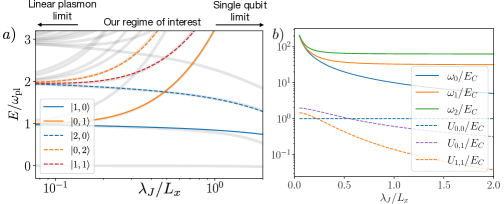
Figure 2: (a) Spectrum of quasi-1D quantum extended Josephson junction as function of the inverse junction length. Gray lines indicate the numerical diagonalization of the exact Hamiltonian restricted to three modes. Colored lines stand for the qubit states of the approximate Hamiltonian Eq. (6), (7). Zero frequency corresponds to $\left|0,0\right\rangle$ state. (b) Qubit energies and Hubbard $U$ of different modes as function of the junction size. We assume the following parameter ratio $\omega_{\text{pl}}/E_{C}=10$ for $\lambda_{J}/L_{x}$=1.

II Extended Josephson junction

We consider a 2D bilayer superconductor, forming an extended Josephson junction, interacting with the electromagnetic field of a resonator, as shown in Fig. 1 (a). We assume that the size of the junction is given by $L_{x}\times L_{y}$ with one of the dimensions ($L_{x}$) being comparable to the wavelength of the cavity field. More importantly, we consider $L_{x}\sim\lambda_{J}$, where $\lambda_{J}$ is the Josephson penetration length that characterizes the stiffness of phase fluctuations in each superconducting region, and which we explicitly define below. In conventional qubits $L_{x}\ll\lambda_{J}$, and one deals with only one Josephson plasmon mode, while in our case, the spatial dependence of the superconducting phase fluctuations cannot be neglected, and one can have many Josephson plasmon modes. In this Section, we derive the complete quantum mechanical description of the multimode Josephson junction and its interaction with the electromagnetic environment.

As shown in Fig. 1 (a), we consider an elongated junction where $L_{x}\gg L_{y}$. The well-known classical description of the junction is given by the sine-Gordon Lagrangian (Kivshar and Malomed, 1989a; Tinkham, 2004):

$$\mathcal{L}_{\text{sG}}=\int\frac{dx}{L_{x}}\left(\frac{1}{16E_{C}}\left(\partial_{t}\theta\right)^{2}-\frac{E_{J}\lambda_{J}^{2}}{2}\left(\partial_{x}\theta\right)^{2}+E_{J}\cos\left(\theta\right)\right),$$ (2)

where $\theta=\theta\left(x,t\right)\equiv\theta_{2}-\theta_{1}+\frac{2e}{c}\int_{1}^{2}{\bf A}d{\bf z}$ denotes the gauge-invariant phase difference between the two superconductors. $E_{C}$ and $E_{J}$ are the total charging energy and Josephson energies, respectively, and $\lambda_{J}$ is the Josephson penetration length $\lambda_{\text{J}}^{2}\equiv\Phi_{0}c/8\pi^{2}(\delta_{z}+2\lambda_{L})j_{c}$, where $j_{c}$ is the critical current of the junction, $\Phi_{0}$ is the flux quantum, $\delta_{z}$ is the distance between superconducting islands (Tinkham, 2004). We note that Eq. (2) can be derived from the quantum mechanical description of a bilayer superconductor, as we demonstrate in App. A. The corresponding Euler-Lagrange equation of motion of the Lagrangian in Eq. 2 is known as the sine-Gordon equation:

$$\partial_{x}^{2}\theta-\tilde{c}^{-2}\partial_{t}^{2}\theta=\lambda_{J}^{-2}\sin(\theta),$$ (3)

where $\tilde{c}^{2}=8E_{C}E_{J}\lambda_{J}^{2}$. We also supplement Eq. 3 with the boundary conditions which are $\partial_{x}\theta=0$ at the junction boundary representing the absence of supercurrents outside the superconducting islands. In this case the variation of the phase is small $\delta\theta\ll 2\pi$, we can linearize Eqs. (2, 3) which becomes equivalent to a set of harmonic oscillators. Following this approach, we perform the quantization of the junction below.

II.0.1 Quantization of phase fluctuations

We now quantize the fluctuations of phase in the extended Josephson junction. In the limit when the phase variations are small $\delta\theta\ll 1$, we expand the cosine term in Eq. (2) as $\cos\left(\theta\right)\approx 1-\theta^{2}/2+\theta^{4}/24$. Our goal is now to quantize the phase fluctuations keeping only up to the quadratic term. We then treat the higher-order terms in Eq. (2) as perturbation. We note that throughout this work we will assume the junction size is of the order of several Josephson lengths. In this case, we can safely neglect the spontaneous (thermal) nucleation of vortices as we discuss in App. D.

We expand the phase over a complete set of modes as eigenmodes of the differential operator $(-\partial_{x}^{2}+\lambda_{J}^{-2})$ with the appropriate boundary condition as $\theta=\sum_{m}\theta_{m}\Xi_{m}\left(x\right)$, where $\int_{-L_{x}/2}^{L_{x}/2}\Xi_{m}\left(x\right)\Xi_{m^{\prime}}\left(x\right)dx=L_{x}\delta_{m,m^{\prime}}$. By performing the Legendre transformation, we get the classical quadratic and quartic Hamiltonians:

$$H^{(2)} =\sum_{m}\left\{4E_{C}\pi_{m}^{2}+\frac{1}{16E_{C}}\omega_{m}^{2}\theta_{m}^{2}\right\},$$ (4)

$$H^{(4)} =-\frac{E_{J}}{24}\int\frac{dx}{L_{x}}\left(\sum_{m}\Xi_{m}\left(x\right)\theta_{m}\right)^{4},$$ (5)

where $\pi_{m}$ is the momentum and we defined the mode frequency $\omega_{m}=\omega_{{\rm{pl}}}\sqrt{1+\lambda_{J}^{2}\left(\frac{\pi m}{L}\right)^{2}}$, and the plasmon frequency $\omega_{{\rm{pl}}}\equiv\sqrt{8E_{J}E_{C}}$. Eq. (4) is equivalent to a set of harmonic oscillators and can perform quantization of harmonic oscillators in Eq. (4). The quantization of Eq. (2) can be performed in a standard way:

$$\hat{H}^{(2)}=\sum_{m}\frac{\omega_{m}}{2}\left(\hat{\pi}_{m}^{2}+\hat{\theta}_{m}^{2}\right)=\sum_{m}\omega_{m}\hat{b}_{m}^{\dagger}\hat{b}_{m},$$ (6)

where we defined the phase fluctuation and its canonical conjugate operators are denoted as $\hat{\theta}_{m}=\sqrt{\frac{4E_{C}}{\omega_{m}}}(\hat{b}_{m}^{\dagger}+\hat{b}_{m})$, $\hat{\pi}_{m}=\sqrt{\frac{\omega_{m}}{16E_{C}}}$$(i\hat{b}_{m}^{\dagger}-i\hat{b}_{m})$ with $\hat{b}_{m}^{\dagger}/\hat{b}_{m}$ being the creation/annihilation operators of $m-$th mode $[\hat{b}_{m},\hat{b}_{m^{\prime}}^{\dagger}]=\delta_{m,m^{\prime}}$. The zero-point fluctuations of the phase operator are thus given by $\theta_{\text{ZPF}}=\sqrt{4E_{C}/\omega_{m}}$. For the validity of the quantization in this section, we need $\theta_{\text{ZPF}}\ll 1$, which is satisfied since we consider $E_{J}\gg E_{C}$.

II.0.2 Nonlinearity

We now discuss the quantization of non-linearity of the multiple modes of Eq. (5). We note that the ambiguity in the operator ordering can be lifted in the microscopic derivation of the fully quantum mechanical action of the junction as we present in App. A. Here, for simplicity, we simply extend the derivation of the single-mode junction (Blais et al., 2021), to the multimode case of interest. Neglecting the excitation non-conserving terms, the nonlinear part of the Hamiltonian becomes:

$$\hat{H}^{(4)} \approx-\frac{U_{0,0}}{2}\hat{b}_{0}^{\dagger}\hat{b}_{0}^{\dagger}\hat{b}_{0}\hat{b}_{0}-\frac{U_{1,1}}{2}\hat{b}_{1}^{\dagger}\hat{b}_{1}^{\dagger}\hat{b}_{1}\hat{b}_{1}$$

$$-U_{0,1}\left(\hat{b}_{1}^{\dagger}\hat{b}_{1}\hat{b}_{0}^{\dagger}\hat{b}_{0}+\frac{1}{4}\hat{b}_{0}^{\dagger 2}\hat{b}_{1}^{2}+\frac{1}{4}\hat{b}_{1}^{\dagger 2}\hat{b}_{0}^{2}\right).$$ (7)

In the limit $L_{x}\sim\lambda_{J}$, the first several terms are found to be $U_{0,0}=E_{C},$ $U_{0,1}=2E_{C}$ and $U_{1,1}=3E_{C}/2$. We note that in Eq. (7), we ignored the linear terms that renormalize the plasmon frequencies. In the case of a finite ratio $L_{x}/\lambda_{J}$, the nonlinearity coefficients depend on the junction size as shown in Fig. 2(a). The three terms in the equation above respectively represent the self-, cross-Kerr, and parametric interaction terms. As shown in Fig. 2(b), the strengths of these various different terms strongly depend on the size of the junction. For larger junction sizes, the spacing between qubit frequencies is decreasing, and the interaction strengths ($U$’s) are decreasing. We note that the charge sensitivity (Koch et al., 2007) is inversely proportional to the phase uncertainty, and for our choice of parameters (also known as the transmon regime $E_{J}\gg E_{C}$) it is negligible.

In addition to the Kerr and cross-Kerr terms in Eq. (7), the terms involving three and four different modes are allowed by the symmetry of the junction $\hat{H}^{\prime(4)}\approx-U_{0,1,2}\hat{X}_{2}\hat{X}_{1}^{2}\hat{X}_{0}$, $\hat{H}^{\prime\prime(4)}\approx-U_{0,1,2,3}\hat{X}_{3}\hat{X}_{2}\hat{X}_{1}\hat{X}_{0}$ with $\hat{X}_{i}\equiv b_{n}+b_{n}^{\dagger}$. In the limit $L_{x}/\lambda_{J}\gg 1$, we find $\chi_{0,1,2}\approx E_{C}/\sqrt{2}$ and $\chi_{0,1,2,3}\approx E_{C}\sqrt{2}$. We note that the plasmon frequencies $\omega_{m}$ are generally incommensurate, and therefore $H^{\prime(4)}$ and $H^{\prime\prime(4)}$ terms are excitation non-preserving. However, one can make these terms resonant by driving, where the energy mismatch is compensated by an external driving as we discuss in the Sec. IV.

III Coupling to the electromagnetic field

We proceed to examine the interaction between the extended JJ modes, derived in the previous Section, and the electromagnetic field of a microwave resonator, as depicted in Fig. 1 (a). Our focus is on the interaction with the $E^{(z)}$ field component, which induces a voltage across the junction. In the classical picture, the external voltage bias can be taken into account on the level of Lagrangian formulation Eq. (2) by the following substitution $\partial_{t}\theta\rightarrow\partial_{t}\theta+2e\int_{1}^{2}dzE^{(z)}$. By performing the Legendre transformation of the resulting Lagrangian as discussed in App. A.4, we get the classical coupling Hamiltonian $H_{\text{int}}=2e\delta_{z}\sum_{n}\pi_{m}E_{m}^{(z)}$, where the overlap of the electric field and the $m$-th plasmon mode profile is defined as $E_{m}^{(z)}\equiv\int\frac{dx}{L_{x}}E^{(z)}\left(x\right)\Xi_{m}\left(x\right)$. In the following, we assume this coupling is weak such that we can separately quantize the electromagnetic field and the superconductor.

Initially, we examine the quantization of transverse electromagnetic (TEM) modes in the electromagnetic field of a coplanar resonator shown in Fig. 1 (a). We assume the resonator length along $x$ direction as $L^{\text{res}}$. We do not discuss the quantization procedure as it can be found in e.g. Blais et al. (2021). The quantized operator of the electromagnetic field takes the standard form (Kakazu and Kim, 1994; Grynberg et al., 2010):

$$\hat{E}^{(z)}(x)=\sum_{n}E_{n}^{0}(i\hat{a}_{n}{\cal E}_{n}\left(x\right)+\text{H.c.}),$$ (8)

where ${\cal E}_{n}$$\left(x\right)$, $\omega_{n}^{\text{res}}$, respectively denote the electromagnetic mode profile and the frequency of $i$-th resonator mode. $E_{n}^{0}$ is the zero-point electric field of $n$-th mode of the resonator. In this section, we restrict our consideration to a homogeneous field distribution along $y$ and $z$ directions in Eq. (8) for simplicity. The total Hamiltonian of the EM field is given by $H_{\text{EM}}=\sum_{n\geq 0}\omega_{n}^{\text{res}}a_{n}^{\dagger}a_{n}$ with $\omega_{n}^{\text{res}}=\pi(n+1)c/L^{\text{res}}$. In Eq. (8), we only considered the electromagnetic field with a polarization component along $\hat{z}$ direction that induces a voltage across the junction. Here we assume the zero voltage boundary conditions which can be achieved by grounding the end points of the resonator (Bothner et al., 2013).

The quantized coupling to the Josephson junction can be obtained from the classical Hamiltonian $H_{\text{int}}$ by simply replacing fields with the corresponding operators. Ignoring the excitation-non-preserving terms, we get:

$$\hat{H}_{\text{int}}=\sum_{m,n}g_{m,n}\hat{a}_{n}\hat{b}_{m}^{\dagger}+\text{H.c.},$$ (9)

where the qubit-photon couplings are $g_{m,n}=2e\delta_{z}E_{n}^{0}\sqrt{\frac{\omega_{m}}{16E_{C}}}\int\frac{dx}{L_{x}}{\cal E}_{n}\left(x\right)\Xi_{m}\left(x\right)$ and $\delta_{z}$ denotes the distance between the superconducting layers. We note that our description of light-matter coupling is a simplified one, and in realistic scenarios, the effective thickness $\delta_{z}$ is determined by a combination of many factors, including the geometry of capacitors, and it is not equal to the distance between superconducting islands. The most reliable approach for determination of the coupling coefficients $g_{m,n}$ is based on the finite element methods Koch et al. (2007).

These couplings can be evaluated in a general case but it is useful to consider a configuration where some of the couplings vanish for symmetry reasons. In particular, if the junction is placed in the center of the resonator, some of the coupling coefficients vanish due to the selection rules imposed by the inversion symmetry with respect to $x$-axis. Specifically, we have $g_{m,n}\neq 0$, if $m$, $n$ are both odd or even. The effective circuit description of such a junction-resonator configuration is shown in Fig. 1 (b). The multimode structure of an extended junction enables the encoding of multiple qubits within a single junction. Mode-selective coupling to the electromagnetic field serves as a versatile tool for manipulating the quantum state, as depicted in Fig. (1) (c), where we schematically illustrate all the possible couplings between the Fock states of the junction and the resonator allowed for by Eq. (9). On a semiclassical level, our coupling can be used to characterize the nonlinearity of the junction itself as discussed in App. E.

IV Quantum simulation with extended Josephson junctions

In the following section, we aim to illustrate the wide-ranging capabilities of our setup. We show that our system functions as a complete toolbox for simulating many-body physics and lattice gauge theories. In particular, we examine a system of $N$ extended Josephson junctions interacting with the electromagnetic field within a resonator, as depicted in Fig. 3 (a). We further assume that these junctions are subjected to external driving, and as we will demonstrate later, this can result in excitation tunneling in a synthetic dimension that is parameterized by $m$. We focus exclusively on the interaction of each junction with the resonator, neglecting potential direct capacitive (dipole-dipole) couplings between the junctions. This assumption is valid as long as the distance between any pair of junctions is greater than the distance between JJs and the waveguides. Expanding to a multi-junction setup and incorporating their connection to the waveguide can be achieved, by adhering to the derivation outlined in Sec. (III). By denoting the creation/annihilation operators of the $i$-th junction by $b_{m}^{(i)\dagger}/b_{m}^{(i)}$, we express the full Hamiltonian $H=H_{\text{q}}+H_{\text{nl}}+H_{\text{tun}}+H_{\text{tun}}^{\prime}$:

$$H_{\text{q}} =\sum_{m}\omega_{m}b_{m}^{(i)\dagger}b_{m}^{(i)},$$ (10)

$$H_{\text{nl}} =-\sum_{m,n,i}U_{m,n}\hat{b}_{m}^{(i)\dagger}\hat{b}_{n}^{(i)\dagger}\hat{b}_{n}^{(i)}\hat{b}_{m}^{(i)},$$ (11)

$$H_{\text{tun}} =-\sum_{i,j,m}t_{i,j}^{(m)}b_{m}^{(i)\dagger}b_{m}^{(j)}+\text{H.c.},$$ (12)

$$H_{\text{tun}}^{\prime} =-\sum_{i,m,m^{\prime}}t_{i}^{\prime(m,m^{\prime})}b_{m}^{(i)\dagger}b_{m^{\prime}}^{(i)}+\text{H.c.},$$ (13)

whereas before we ignore the excitation-non-preserving terms. The first two terms $H_{{\bf q}}$ and $H_{\text{nl}}$ stand for the Hamiltonians of each junction while $H_{\text{tun}}$ and $H_{\text{tun}}^{\prime}$ correspond to the different excitation tunneling processes that will be discussed below.

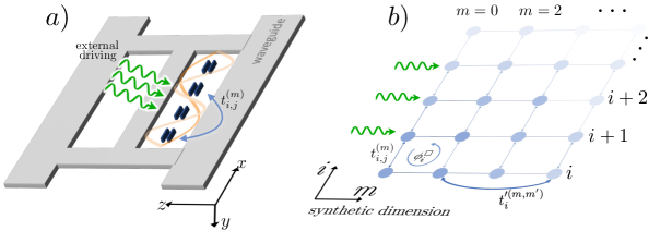
Figure 3: Implementation of multi-component Bose-Hubbard model with an array of extended Josephson junctions. (a) Schematic representation of an array of 4 extended JJ is placed in a resonator. $n=2$ and $n=4$ resonator modes are shown in orange and pale orange respectively. Each junction is placed in an anti-node of $n=4$ mode. (b) Equivalent Bose-Hubbard model in synthetic dimension. For schematic simplicity the junctions are shown with layers stretched along $z$ direction, i.e. along the dominant electric field of the resonator. The actual experimentally motivated geometry is shown in Fig. 5.

We begin with a discussion of the Hamiltonian equation denoted as Eq. (13), which corresponds to the tunneling of an excitation between different junctions, mediated by the waveguide. The microscopic representation of this process is encapsulated by the Hamiltonian $H_{\text{int}}=\sum_{m,n,i}g_{m,n}^{(i)}a_{n}b_{m}^{(i)\dagger}+\text{H.c.}$ which is an elaboration of Eq. (9), adapted to accommodate scenarios involving multiple junctions. Adiabatically eliminating the resonator modes, we get Eq. (13) with the detuning denoted as $\delta_{m,n}=\omega_{m}-\omega_{n}^{\text{res}}$ and $t_{i,j}^{(m)}=\sum_{n}g_{m,n}^{(j)}g_{m,n}^{(i)}/\delta_{m,n}$, where the summation is taken over all the resonator modes parametrized by $n$. We note that $t_{i,j}^{(m)}$ is proportional to the Green’s function describing the photon propagation between two junctions $i$ and $j$, where its specific form depends on the waveguide configuration. For example, in the configuration shown in Fig. (3) (a), the tunneling coefficient $t_{i,j}^{(m)}$ can be expected to be of long- (infinite) range character. We note that the tunneling can become short-range in the case of each junction coupled to its own resonator in a resonator array as in (Houck et al., 2012; Schmidt and Koch, 2013; Sundaresan et al., 2019; Mirhosseini et al., 2018). To maximize tunneling and consequently the achievable quantum simulation times, it is beneficial to minimize the detuning between plasmon and cavity modes. One approach for achieving this is through the adjustment of the junction geometry. Specifically, selecting the appropriate junction length can adjust the spacing between plasmon modes, as follows from Eq. (1). Alternatively, the plasmon frequencies can be adjusted via external driving such as to induce AC Stark frequency shifts.

The last term, $H_{\text{tun}}^{\prime}$, characterizes the resonant excitation exchange among different plasmon modes inside one junction, which, as we show below, can be induced by an external driving. As a specific example, we now outline a protocol for implementing the tunneling between $m=0$ and $m=2$ junction modes, keeping in mind that a similar approach could be used to induce tunneling between other odd pairs of modes. In particular, we consider a weak drive for the $m=1$ mode described by the RWA Hamiltonian $H_{\text{dr}}(t)=\alpha_{1}\sum_{i}(\hat{b}_{1}^{(i)}e^{i\omega_{1}^{\text{dr}}t+i\phi_{i}}+\hat{b}_{1}^{(i)\dagger}e^{-i\omega_{1}^{\text{dr}}t-i\phi_{i}}$) with $\omega_{1}^{\text{dr}}=(\omega_{2}-\omega_{0})/2$ and $\phi_{i}$ denotes the driving phase of $i$-th junction and $\alpha_{1}$ is the effective Rabi frequency. The selective excitation of a single mode can be realized through the momentum or frequency specificity of the coupling. This yields the mean-field quasi-steady-state coherence of the driven mode $\bar{b}_{1}\approx-\alpha_{1}e^{i\phi_{i}}/(\omega_{1}^{\text{dr}}-\omega_{1})$. With this, the tunneling between plasmon modes is induced by the non-linear excitation-non-conserving Hamiltonian $\hat{H}^{\prime(4)}$ (see Sec. II.0.2) that is now driven. We get an effective resonant tunneling $0\leftrightarrow 2$ that is given by Eq. (13) with $t_{i}^{(0,2)}=U_{0,1,2}|\bar{b}_{1}|^{2}e^{-2\phi_{i}}$. This shows that the phase of complex tunneling between same-parity sites is set by drive. Extending $H_{\text{tunn}}^{\prime}$ to all the sites and combining it with $H_{\text{tunn}}$, we find a rich set of tunneling terms in 2D shown in Fig. 3 (b), where one dimension is spatial JJ sites and the other dimension is different plasmon modes, in form of a synthetic dimension. In particular, one can set the drive phases to achieve a non-zero total tunneling phase over a plaquette: $\phi_{i}^{\boxempty}=2\left(\phi_{i}-\phi_{i+1}\right)$ to obtain an artificial gauge field. We summarize by mentioning that our final Hamiltonian is given by Eqs. (10-13) and it represents the multi-component Bose-Hubbard model in an artificial external magnetic field.

The multicomponent Bose-Hubbard model enables the implementation of quantum simulation protocols for intricate many-body phenomena, which we discuss it here. It is worth noting that comparable models have also emerged in the study of conventional Josephson junction arrays as referenced in (Van der Zant et al., 1992; Makhlin et al., 2001), as well as in the examination of arrays of coupled cavities inhabited by multi-level atoms (Hartmann et al., 2008; Kleine et al., 2008). This model is recognized for exhibiting phenomena such as spin components "demixing" (Cazalilla and Ho, 2003) and spin-charge separation (Recati et al., 2003). When subjected to strong interactions, it is anticipated that the Hubbard models will transition to the Mott-insulator state (Cole et al., 2012). In this state, the low-energy dynamics are characterized by the effective spin Heisenberg models represented in different bosonic components (Hartmann et al., 2008). Presenting this system to a synthetic gauge field, as in our situation, can reveal a spectrum of fascinating phenomena, including a Mott insulator state with chiral currents (Dhar et al., 2012) and aspects of quantum Hall physics (Hafezi et al., 2007; Tokuno and Georges, 2014). Furthermore, the glassy phases predicted in a single-component polaritonic Hubbard model are explored in (Rossini and Fazio, 2007). We finish this section by stating that the effective Hubbard model, as presented by Eqs. (10-13), possesses all the necessary elements to perform quantum simulations of lattice gauge theories (Aidelsburger et al., 2022), as recently suggested in (Osborne et al., 2022; Mil et al., 2020).

V Qubit operation

We now discuss the potential application of our setup to implement single and two-qubit gates for quantum computation. We assume the individual addressing of each junction mode by using the parity selection rules as discussed above. The single-qubit rotations can be performed trivially by applying the external microwave tone of the corresponding frequency. Therefore below, we focus only on two-qubit gates. Theoretically, the phase gate can be implemented for any pair of qubits residing in one or separate junctions. Below we focus on the former case as we expect it to have much higher fidelity.

Two-qubit gate —

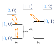
Figure 4: Implementation of an intra-junction two-qubit phase gate. The qubit $b_{0}$ is driven resonantly with the transition $\left|1,0\right\rangle\rightarrow\left|2,0\right\rangle$ for half a period of a corresponding Rabi oscillation picking up a $\pi$ phase. Other transitions are assumed to be off-resonant due to the Kerr and cross-Kerr interaction terms between different junction modes.

We now exemplify the implementation of an intra-junction two-qubit gate ignoring the coupling to the resonator. We operate here with the logical states $|0\rangle,|1\rangle$ of the two lowest modes of the junction $b_{0}$ and $b_{1}$, as shown in Fig. 1 (c). We define the two-qubit phase gate as the unitary transformation: $|i,j\rangle\rightarrow\exp{(i\pi\delta_{i,1}\delta_{j,0})}|i,j\rangle$, where $\delta$ is the Kronecker delta symbol. Such a unitary can be implemented by assuming a field driving that is resonant only with the transition $\left|1,0\right\rangle\rightarrow\left|2,0\right\rangle$. By driving this transition for half of the period of a full Rabi oscillation, the junction state picks up a $\pi$ phase $\left|1,0\right\rangle\rightarrow e^{i\pi}\left|1,0\right\rangle$. In a realistic situation the two other symmetry-allowed transitions $\left|1,0\right\rangle\rightarrow\left|0,0\right\rangle$ and $\left|0,1\right\rangle\rightarrow\left|1,1\right\rangle$ will be driven as well as shown in Fig 4. The detunings of these two transitions are respectively given by the nonlinearity terms $U_{0,0}$ and $U_{1,1}\approx 2U_{0,0}$ in the limit of large junction. Therefore the estimate of the relevant degree of qubit non-linearity can be given in terms of the ratio of the anharmonicity to the qubit decoherence rate $U_{0,0}/\gamma_{\text{d}}$. The estimate of this ratio is provided in the section below.

VI Experimental considerations

We now discuss the experimental parameters of the extended junction described above. Our estimations are based on the physical parameters in Ref. (Mamin et al., 2021). Although a square geometry is employed in that reference, we assume that similar parameters apply to our rectangular geometry. In this section, we will use SI units for experimental purposes, deviating from the Gaussian units employed throughout the rest of the text.

Using the critical current value $j_{c}\approx 10\text{nA/$\mu\text{m}^{2}$}$, where $\epsilon_{0}$ is the vacuum permittivity, and assuming the oxide thickness $\delta_{z}\approx 2\text{nm}$ and the London penetration length of aluminum $\lambda_{L}=16\text{nm}$, we calculate the Josephson length to be $\lambda_{J}\approx\sqrt{\Phi_{0}/2\pi\mu_{0}(\delta_{z}+2\lambda_{L})j_{c}}\approx 880\mu\text{m}$, where $\Phi_{0}$ denotes the flux quantum (Poole et al., 2013).

For the junction area, we assume the following geometric parameters: $S\approx 10\text{nm}\times\lambda_{J}$. Using the above critical current density, we obtain the Josephson energy as $E_{J}=Sj_{c}/2e\approx 2\pi\times 40\text{GHz}$. The charging energy can be determined as $E_{C}\approx\omega_{\text{pl}}^{2}/8E_{J}\approx 2\pi\times 0.06\text{GHz}$, assuming that the fundamental plasmon frequency is not influenced by the geometry and has a value of $\omega_{\text{pl}}\approx 2\pi\times 5\text{GHz}$. The cavity qubit coupling in our toy model can be estimated using the experimentally achievable value of the zero-point electric field $E_{n=0}^{0}=0.2\text{V/m}$ (Wallraff et al., 2004). With this we find the single-photon Rabi frequency $g_{0,0}\approx 3$ MHz (see Appendix A.4).

We also compare our predictions with the results of finite-element numerical simulation using the commercially available software (Ansys Maxwell) for a more realistic geometry. More precisely, we consider two superconducting islands of dimensions $10\times 440\mu\text{m}^{2}$ oriented in the x-z plane one on top of the other with the overlap junction area of $10\text{nm}\times 440\mu\text{m}$ as shown in Fig. 5 a), b). With this we find the following junction parameters $E_{C}=2\pi\times 84$ MHz, $E_{J}\approx 2\pi\times 22$ GHz, $\omega_{\text{pl}}\approx 2\pi\times 3.8$ GHz. We also estimate the qubit - cavity coupling strength to be $g_{0,0}\approx 2\pi\times 24$ MHz. The enhanced coupling strength in this geometry stems from the fact that the superconducting islands are larger than the JJ itself and contribute to effective thickness $\delta_{z}$ (Koch et al., 2007)

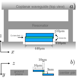
Figure 5: Schematic (not to scale) representation of the long Josephson junction configuration used for the finite-element numerical simulation. a) top view, b) side view. Regions highlighted in green denote the junction area.

As mentioned earlier, larger Josephson junctions (JJs) have smaller nonlinearities and one needs to ensure that the nonlinearity strength (approximately $E_{C}$) remains larger than the dissipation rates. Assuming an energy dissipation time scale of $T_{1}\approx 30\mu s$, we estimate such a ratio to be favorable, with $2\pi E_{C}T_{1}\leavevmode\nobreak\ \sim 10^{4}$.

We note that for larger junction sizes, where $L\sim\lambda_{J}$, an additional imperfection source arises from Josephson vortex nucleation. The corresponding vortex density in equilibrium is given by (Wonneberger, 1980; Kivshar and Malomed, 1989b):

$$\left\langle n\right\rangle=\left(\frac{2}{\pi}\right)^{1/2}\lambda_{J}^{-1}\sqrt{\frac{2E_{J}}{k_{{\rm B}}T}}e^{-2E_{J}/k_{{\rm B}}T}.$$

For the parameters considered, $\left\langle n\right\rangle L_{x}\ll 1$, which indicates that nucleation can be neglected.

VII Conclusions & outlook

In this work, we developed a theoretical framework for describing the light-matter interaction in extended Josephson junctions. We demonstrated that each such junction could host multiple plasmon modes, each encoding a qubit. It is possible to address each qubit mode individually due to the frequency-momentum-selective coupling, which arises from the different profiles of their electronic wavefunctions. We also consider the system of several extended junctions interacting through a single resonator and demonstrate that such a system could be used to simulate an interacting 2D Bose-Hubbard model with one of its dimensions being synthetic. Besides, we also show that the system can be used in order to perform quantum computation. In particular, we proposed the implementation of single- and two-qubit gates inside a single extended Josephson junction. Our work allows us to address several interesting problems in the future, including the possibility of inducing photon-photon interactions in long junctions and generating non-classical states of light. Another interesting direction would be to study the effects of non-trivial junction geometry (topology) on light-matter interactions.

Appendix A Microscopic derivation

In this section we derive the effective action of Josephson junction interacting with the resonator EM field. The setup we have in mind is shown in Fig. 1. In this note to some extent the formalism follows (Altland and Simons, 2010; Sun et al., 2020). We consider the imaginary-time action of two quasi-two-dimensional superconductors $S_{\text{full}}=S_{0}+S_{J}+S_{\text{EM}}$:

$$S_{0} =\sum_{i=1,2}\int d^{2}{\bf r}L_{z}\int_{0}^{\beta}d\tau\left\{\frac{\nu}{2}\left(\partial_{\tau}\theta_{{\bf r}}^{(i)}-e\phi_{{\bf r}}^{\left(i\right)}\right)^{2}+\frac{n_{s}}{2m}\left(\nabla\theta_{{\bf r}}^{\left(i\right)}-\frac{e}{c}{\bf A}_{{\bf r}}^{\left(i\right)}\right)^{2}\right\},$$ (14)

$$S_{\text{J}} =-\frac{E_{\text{J}}}{S}\int d^{2}{\bf r}\int_{0}^{\beta}d\tau\cos 2\left(\theta_{{\bf r}}^{(1)}-\theta_{{\bf r}}^{\left(2\right)}-\frac{e}{c}\int_{1}^{2}d\vec{z}\cdot{\bf A}_{{\bf r},z}\right),$$ (15)

where $\phi_{{\bf r}}^{(i)},{\bf A}_{{\bf r}}^{(i)}$, denotes the values of the scalar and vector potentials at $i$-th layers respectively, $m,e$ are the electron mass and charge respectively, $n_{s}$ denotes the superfluid density. $\theta^{(i)}$ is the phase of $i$-th superconductor. The boundary conditions imposed by resonator can be straightforwardly included into Eqs. 14. In the following we denote the in-plane vectors as ${\bf r}$. The size of each superconductor is assumed to be $L_{x}\times L_{y}\times L_{z}$ such that $L_{z}\ll L_{x,y}$. $E_{\text{J}}$ is the Josephson coupling energy.

We follow the procedure outlined below. We first consider the junction alone and derive its effective action by integrating-out the static components of EM field responsible for the inductive and charging interaction between superconductors. We then add the interaction with the electromagnetic resonator modes perturbatively in a gauge-invariant way with the only assumption that resonator does not affect the Lorentz and Coulomb force between superconductors.

A.1 Josephson junction action

We now define the symmetric and the anti-symmetric phase variable as follows $\theta_{{\bf r}}^{\left(\pm\right)}=2\left(\theta_{{\bf r}}^{(1)}\pm\theta_{{\bf r}}^{(2)}\right)$ and we integrate-out the static parts of vector and scalar potentials (see below) in Eqs. (14-15). We find the following action:

$$S_{0} \approx\int\frac{d^{2}{\bf r}}{S}d\tau\left\{\frac{1}{16E_{C}}\left(\partial_{\tau}\theta_{{\bf r}}^{(-)}\right)^{2}+\frac{E_{\text{J}}\lambda_{\text{J}}^{2}}{2}\left(\vec{\nabla}\theta_{{\bf r}}^{\left(-\right)}\right)^{2}\right\}$$ (16)

$$S_{\text{J}} \approx-\frac{E_{\text{J}}}{S}\int d^{2}{\bf r}d\tau\cos\left(\theta_{{\bf r}}^{(-)}\right)$$ (17)

where $E_{C}$ is the total charging energy and $\lambda_{\text{J}}^{2}\equiv\Phi_{0}c/8\pi^{2}\delta_{z}j_{c}$ is the Josephson penetration length and $S$ is the surface are of the junction. $\Phi_{0}$ denotes the flux quantum and $j_{c}$ is the critical current through the junction which we assume to be constant. The $+$ component of the field becomes gapped and is neglected in the action above. We note that the Josephson term 17 is only valid at lengthscales larger than the coherence length $k^{-1}\gg v_{F}/\Delta$ where $\Delta$ is the gap of the superconductor and $v_{F}$ is the Fermi velocity.

A.2 Quantized phase fluctuations

In this section we derive the Hamiltonian of the effective Josephson qubit. We first expand the action Eqs. 16-17 up to quartic term and get:

$$S^{\left(2\right)} \approx\frac{1}{16E_{C}S}\int d^{2}{\bf r}d\tau\theta_{{\bf r}}^{\left(-\right)}\left\{-\partial_{\tau}^{2}+\omega_{\text{pl}}^{2}\left\{1-\lambda_{\text{J}}^{2}\vec{\nabla}^{2}\right\}\right\}\theta_{{\bf r}}^{\left(-\right)}$$ (18)

$$S^{\left(4\right)} \approx-\frac{1}{24}\frac{E_{\text{J}}}{S}\int d^{2}{\bf r}d\tau\theta_{{\bf r}}^{(-)4}$$ (19)

where the Josephson plasmon frequency is $\omega_{\text{pl}}=\sqrt{8E_{\text{C}}E_{\text{J}}}$. If we neglect the fact that $\theta$ is the angle variable and treat it as a bosonic field then the linear part of the action Eq. 18 represents the set of harmonic oscillators. We now expand the phase field over eigensystem of the $\left\{1-\lambda_{\text{J}}^{2}\vec{\nabla}^{2}\right\}$ operator with the boundary conditions $\nabla\theta^{\left(-\right)}=0$:

$$\theta_{{\bf r}}^{\left(-\right)}\left(\tau\right)\equiv\sum_{m}\sqrt{\frac{4E_{\text{C}}}{\omega_{m}}}\Xi_{m}\left({\bf r}\right)\theta_{m}\left(\tau\right),$$ (20)

where $\left\{1-\lambda_{\text{J}}^{2}\vec{\nabla}^{2}\right\}\Xi_{m}\left({\bf r}\right)\equiv\epsilon_{m}^{2}\Xi_{m}\left({\bf r}\right)$ and we assumed the normalization condition $\int d^{2}{\bf r}\Xi_{m}\left({\bf r}\right)\Xi_{m^{\prime}}\left({\bf r}\right)=S\delta_{m,m^{\prime}}$, where $S$ is the junction surface. The prefactor in Eq. (20) guarantees the proper normalization of the phase fluctuations. From now on we focus on a “long” rectangular Josephson junction, i.e. we consider $L_{x}\gg L_{y}$. Assuming $x\in[\frac{L_{x}}{2},\frac{L_{x}}{2}]$ we can restrict the modes to $\Xi_{m}(x,y)\approx\Xi_{m}\left(x\right)=\sqrt{2}\sin\frac{\pi x}{L_{x}}m$ for $m$ being odd, $\Xi_{m}\left(x\right)=\sqrt{2}\cos\frac{\pi x}{L_{x}}m$ for m being even and $\Xi_{m=0}\left(x\right)=1$. The oscillator energies are given by

$$\omega_{m}=\omega_{\text{pl}}\sqrt{\lambda_{\text{J}}^{2}\left(\frac{\pi}{L_{x}}m\right)^{2}+1}.$$

Substituting Eq. (20) to Eq. (18) we can infer the effective linear Hamiltonian (we just replace the fluctuating field with bosonic variables as $\theta_{m}\rightarrow b_{m}+b_{m}^{\dagger}$, where $\left[a_{m},a_{m^{\prime}}^{\dagger}\right]=\delta_{m,m^{\prime}}$ ):

$$H^{(2)}=\sum_{m}\epsilon_{m}b_{m}^{\dagger}b_{m}$$

The quartic term depends on the junction parameters. Below we derive the expression for the junction assuming $L_{x}\gg L_{y}$ for simplicity.

A.3 Extended Josephson junction

We now derive the nonlinear term for the junction assuming $L_{x}\gg L_{y}$. We note that the quadratic part of the Hamiltonian corresponding to Eq. (19) has divergent contributions. In particular, the correction to the 0-th plasmon mode has the following form $E_{C}\left(\sum_{n\geq 0}1/\sqrt{1+\lambda_{J}^{2}\left(\frac{\pi n}{L}\right)^{2}}\right)$, where the sum taken is over all modes. The contribution to the rest modes is found to be $1/\sqrt{1+\lambda_{J}^{2}\left(\frac{\pi n}{L}\right)^{2}}E_{C}\left(\frac{1}{2}+\sum_{m\geq 0}1/\sqrt{1+\lambda_{J}^{2}\left(\frac{\pi m}{L}\right)^{2}}\right)$. The mode cut-off has to be imposed to get a convergent expression. Such cut-off can be obtained on the physical grounds by e.g. demanding the momentum of the contributing mode to be smaller than the coherence length of the superconductor. Here we simply absorb the formally divergent sum into the plasmon frequency definition. In this case, the result is cut-off independent. Below we restrict our consideration to just the two lowest plasmon modes.

Restricting to the lowest two modes we find the expression for the quartic term corresponding to the nonlinear part of the action Eq. (19):

$$H^{(4)} =\frac{E_{C}}{12}\int_{0}^{L_{x}}\frac{dx}{L_{x}}\left\{\sqrt{\frac{\omega_{\text{pl}}}{\epsilon_{0}}}X_{0}+\sqrt{\frac{2\omega_{\text{pl}}}{\epsilon_{1}}}\cos\left(\frac{\pi}{L_{x}}x\right)X_{1}\right\}^{4}$$

$$=\frac{E_{C}}{12}\left\{X_{0}^{4}+6\frac{\omega_{\text{pl}}}{\epsilon_{1}}X_{0}^{2}X_{1}^{2}+\left(\frac{\omega_{\text{pl}}}{\epsilon_{1}}\right)^{2}\frac{3X_{1}^{4}}{2}\right\}$$ (21)

where we neglected quadratic terms and $X_{i}\equiv b_{i}+b_{i}^{\dagger}$. The Hamiltonian Eq. (21) can be simplified even further assuming that the non-linearity is weak compared to the plasma frequency $\omega_{\text{pl}}\ll E_{C}$. In this limit the excitation-number-non conserving terms in $H^{(4)}$ are strongly off-resonant and can be safely neglected:

$$H^{(4)} \approx-\frac{E_{C}}{4}\left\{2b_{0}^{\dagger}b_{0}^{\dagger}b_{0}b_{0}+3b_{1}^{\dagger}b_{1}^{\dagger}b_{1}b_{1}\right.$$

$$\left.+8b_{1}^{\dagger}b_{1}b_{0}^{\dagger}b_{0}+2\left(b_{0}^{\dagger 2}b_{1}^{2}+b_{1}^{\dagger 2}b_{0}^{2}\right)\right\}$$

where we assumed $L_{x}/\lambda_{J}\gg 1$. In conclusion we note that we find interaction terms corresponding to the self-, cross-Kerr and parametric interactions between different modes.

A.4 Interaction with the resonator mode

We now consider the interaction with the resonator mode assuming the geometry shown in Fig. 1. Ignoring the magnetic effects we add the coupling in the gauge-invariant way to the $\partial_{\tau}\theta^{\left(-\right)}\rightarrow\partial_{\tau}\theta^{\left(-\right)}-2ie\int_{1}^{2}d\vec{z}\cdot{\bf E}^{\text{res}}$ action Eq. (15):

$$S_{0} \approx\int\frac{d^{2}{\bf r}}{S}d\tau\left\{\frac{1}{16E_{C}}\left(\partial_{\tau}\theta^{\left(-\right)}-2ie\int_{1}^{2}d\vec{z}\cdot{\bf E}^{\text{res}}\right)^{2}+\frac{E_{\text{J}}\lambda_{\text{J}}^{2}}{2}\left(\vec{\nabla}\theta_{{\bf r}}^{\left(-\right)}\right)^{2}\right\}$$

Following the main text we now first reduce the action to the 1-dimensional form and perform the expansion eigenmode expansion $\theta^{\left(-\right)}\left(x\right)=\sum_{n}\theta_{n}^{(-)}\Xi_{n}\left(x\right)$. With this we get:

$$S_{0} \approx\int d\tau\sum_{m}\left\{\frac{1}{16E_{C}}\left(\partial_{\tau}\theta_{m}^{(-)}\partial_{\tau}\theta_{m}^{(-)}-4ie\partial_{\tau}\theta_{m}^{(-)}\int_{1}^{2}d\vec{z}\cdot{\bf E}_{m}^{\text{res}}-4e^{2}\int\frac{dx}{L_{x}}d\tau\left(\int_{1}^{2}d\vec{z}\cdot{\bf E}^{\text{res}}\right)^{2}\right)\right\}$$

$$+\int\frac{dx}{L_{x}}d\tau\left\{\frac{E_{\text{J}}\lambda_{\text{J}}^{2}}{2}\left(\vec{\nabla}\theta_{{\bf r}}^{\left(-\right)}\right)^{2}\right\},$$

where ${\bf E}_{m}^{\text{res}}\equiv\int\frac{dx}{L_{x}}{\bf E}^{\text{res}}\Xi_{m}\left(x\right)$. We now have to deduce the quantum Hamiltonian of the resonator+junction system which generates the action above. Due to the linearity, the easiest way to extract the coupling is to perform Legendre transform:

$$\pi_{m}^{(-)}=\frac{1}{8E_{C}}\partial_{\tau}\theta_{m}^{(-)}-\frac{1}{4E_{C}}\left(ie\int_{1}^{2}d\vec{z}\cdot{\bf E}_{m}^{\text{res}}\right)$$

With this we get the coupling Hamiltonian:

$$\hat{H}_{\text{int}}=2e\int_{1}^{2}d\vec{z}\cdot\hat{{\bf E}}_{m}^{\text{res}}\hat{\pi}_{m}$$

The Hamiltonian $H_{\text{int}}$ is very general in the sense that it is valid regardless of the details of the system. In realistic scenarios its evaluation represents a complicated problem which requires taking into account e.g. near-field effects (see Sec. VI). In the current section we resort to a simplified parallel-plate geometry. We note that in addition we get terms acting on the electromagnetic field degrees of freedom only. In the following we assume these terms are absorbed in the definition of the resonator mode frequency.

Now using the expression for the quantized oscillator momentum and the resonator mode operator Eq. (8) we get:

$$\hat{H}_{\text{int}}\approx 2e\delta_{z}\sum_{n}E_{n}^{0}\sqrt{\frac{\omega_{m}}{16E_{C}}}(i\hat{a}_{n}{\cal E}_{n,m}+\text{H.c.})(i\hat{b}_{m}^{\dagger}-i\hat{b}_{m}),$$

where the interaction form-factors are denoted as ${\cal E}_{n,m}\equiv\int_{-L_{x}/2}^{L_{x}/2}\frac{1}{L_{x}}{\cal E}_{n}\left(x\right)\Xi\left(x\right)$. In the following we will assume ${\cal E}_{n}\left(x\right)=\sin(\frac{\pi nx}{L_{\text{res}}})$ for $n$ being odd and ${\cal E}_{n}\left(x\right)=\cos(\frac{\pi nx}{L_{\text{res}}})$ for even $n$. In particular, assuming the junction is located exactly in between the centre of the resonator we get for several low-energy modes:

$${\cal E}_{0,0} =\frac{\sin(\tilde{L})}{\tilde{L}}$$

$${\cal E}_{1,1} =\frac{8\sqrt{2}\pi\tilde{L}\cos\left(2\tilde{L}\right)}{\pi^{2}-16\tilde{L}^{2}}$$

$${\cal E}_{2,2} =\frac{3\sqrt{2}\tilde{L}\sin\left(3\tilde{L}\right)}{\pi^{2}-9\tilde{L}^{2}},$$

where $\tilde{L}=L\pi/(2L_{\text{res}})$. With this, we find the coupling terms $g_{m,n}$ in (9) as

$$g_{m,n}=2e\delta_{z}E_{n}^{0}\sqrt{\frac{\omega_{m}}{16E_{C}}}{\cal E}_{m,n}.$$

It is convenient to represent this expression as a product of an effective dipole moment of $m-$th mode $d_{m}=2e\delta_{z}{\cal E}_{m,n}$ and a zero-point value of electric field in $n-$th field mode $E_{n}^{0}$.

Appendix B Derivation of the effective action Eq. (16-17)

In this appendix we provide the microscopic derivation of the effective action Eqs. (14, 15).

B.1 Derivation of the effective action

We now consider the bilayer action Altland and Simons (2010); Sun et al. (2020):

$$S_{0} =\sum_{i=1,2}\int d^{2}{\bf r}L_{z}d\tau\left\{\frac{\nu}{2}\left(\partial_{\tau}\theta_{{\bf r}}^{(i)}+e\phi_{{\bf r}}^{\left(i\right)}\right)^{2}+\frac{n_{s}}{2m}\left(\vec{\nabla}\theta_{{\bf r}}^{\left(i\right)}-\frac{e}{c}\vec{A}_{{\bf r}}^{\left(i\right)}\right)^{2}\right\},$$

$$S_{\text{J}} =-\frac{E_{\text{J}}}{S}\int d^{2}{\bf r}d\tau\cos\left\{2\left(\theta_{{\bf r}}^{(1)}-\theta_{{\bf r}}^{(2)}-\frac{e}{c}\int_{1}^{2}d\vec{z}\cdot\vec{A}_{{\bf r},z}\right)\right\},$$

Let us now transform into the $\pm$ basis by defining new variables for all the fields $X^{\pm}\equiv X^{(1)}\pm X^{(2)}$:

$$S_{0} =\sum_{i=\pm}\int d^{2}{\bf r}L_{z}d\tau\left\{\frac{\nu}{4}\left(\partial_{\tau}\theta_{{\bf r}}^{(i)}+e\phi_{{\bf r}}^{\left(i\right)}\right)^{2}+\frac{n_{s}}{4m}\left(\vec{\nabla}\theta_{{\bf r}}^{\left(i\right)}-\frac{e}{c}\vec{A}_{{\bf r}}^{\left(i\right)}\right)^{2}\right\}$$

The “-” variable we redefine in a gauge-invariant way $\theta_{{\bf r}}^{(-)}\rightarrow\theta_{{\bf r}}^{(-)}-\frac{e}{c}\int_{1}^{2}d\vec{z}\cdot\vec{A}_{{\bf r},z}$ by adding and subtracting $\frac{e}{c}\int_{1}^{2}d\vec{z}\cdot\vec{A}_{{\bf r},z}$:

$$S_{0}^{(-)} =\int d^{2}{\bf r}L_{z}d\tau\frac{\nu}{4}\left(\partial_{\tau}\theta_{{\bf r}}^{(-)}+e\phi_{{\bf r}}^{\left(-\right)}+\frac{e}{c}\int_{1}^{2}d\vec{z}\cdot\partial_{\tau}\vec{A}_{{\bf r},z}\right)^{2}$$

$$+\int d^{2}{\bf r}L_{z}d\tau\frac{n_{s}}{4m}\left(\vec{\nabla}\theta_{{\bf r}}^{\left(-\right)}-\frac{e}{c}\vec{A}_{{\bf r}}^{\left(-\right)}+\frac{e}{c}\int_{1}^{2}d\vec{z}\cdot\nabla_{r}\vec{A}_{{\bf r},z}\right)^{2}$$

and the Josephson term reads:

$$S_{\text{J}}=-\frac{E_{\text{J}}}{S}\int d^{2}{\bf r}d\tau\cos\left\{2\theta_{{\bf r}}^{(-)}\right\},$$

We now use the following two relations which are straightforwardly found using definitions of the scalar and vector potentials:

$$e\phi_{{\bf r}}^{\left(i\right)}+\frac{e}{c}\int_{1}^{2}d\vec{z}\cdot\partial_{\tau}\vec{A}_{{\bf r},z}=-ie\int_{1}^{2}d\vec{z}{\bf E}$$

and

$$\frac{e}{c}\int_{1}^{2}dz\left[{\bf B}\times{\bf e}_{z}\right]-\frac{e}{c}\vec{A}_{{\bf r}}^{\left(-\right)}+\frac{e}{c}\int_{1}^{2}d\vec{z}\cdot\nabla_{r}\vec{A}_{{\bf r},z}=\frac{e}{c}\int_{1}^{2}dz\left[{\bf B}\times{\bf e}_{z}\right]$$

With this we get:

$$S_{0}^{(-)} =\int d^{2}{\bf r}L_{z}d\tau\left\{\frac{\nu}{4}\left(\partial_{\tau}\theta_{{\bf r}}^{(-)}-ie\int_{1}^{2}d\vec{z}\cdot{\bf E}\right)^{2}+\frac{n_{s}}{4m}\left(\vec{\nabla}\theta_{{\bf r}}^{\left(-\right)}+\frac{e}{c}\int_{1}^{2}dz\left[{\bf B}\times{\bf e}_{z}\right]\right)^{2}\right\}$$

In order to get the action of the junction alone we now integrate-out the electromagnetic field by simply solving the Maxwell equations. We assume that the superconductors are located sufficiently close such that the retardation can be ignored. Denoting two fields $\int_{1}^{2}dzE_{{\bf r}}^{(z)}$ and $\int_{1}^{2}dz\left[{\bf B}\times{\bf e}_{z}\right]$ we can find the bare correlation functions according to the Maxwell equations:

$$D_{0,q} \equiv-\left\langle i\int_{1}^{2}d\vec{z}E_{{\bf q}}^{(z)}i\int_{1}^{2}dzE_{-{\bf q}}^{(z)}\right\rangle\approx 2\int_{1}^{2}dz\int_{1}^{2}dz^{\prime}dk_{z}e^{ik_{z}\left(z-z^{\prime}\right)}\left(\frac{k_{z}^{2}}{q_{x}^{2}+k_{z}^{2}}\right)$$

$$\approx 4\frac{\pi}{q}\left(1-e^{-q\delta_{z}}\right)\approx 4\pi\delta_{z}$$

$$D_{q} \approx\left\langle\int_{1}^{2}dz\left[{\bf B}_{{\bf q}}\times{\bf e}_{z}\right]_{{\bf q}}\int_{1}^{2}dz\left[{\bf B}_{-{\bf q}}\times{\bf e}_{z}\right]_{-{\bf q}}\right\rangle\approx 4\pi\delta_{z}$$

The cross-correlation-term yields terms linear in frequency and it can be ignored at low energies.

B.1.1 EM field integrated-out

We now integrate-out the EM field. The resulting action reads:

$$S_{0}^{\left(-\right)}=\frac{1}{2}\sum_{q,\epsilon_{n}}\left\{L_{z}\frac{\nu}{2}\epsilon_{n}^{2}\left(\frac{1}{L_{z}\frac{\nu e^{2}}{2}D_{0,q}^{\left(\pm\right)}+1}\right)\theta_{{\bf q},n}^{(-)}\theta_{-{\bf q},-n}^{(-)}+L_{z}\frac{n_{s}}{2m}\left(\frac{1}{L_{z}\frac{n_{s}}{2m}\left(\frac{e}{c}\right)^{2}D_{q}^{\left(\pm\right)}+1}\right){\bf q}^{2}\theta_{{\bf q},n}^{(-)}\theta_{-{\bf q},-n}^{\left(-\right)}\right\}$$

The $+$ component is of higher order in space-time derivatives and we ignore it. We only keep the “-” component which at low energy becomes:

$$S_{0}^{\left(-\right)}=\frac{1}{2}\sum_{q,\epsilon_{n}}\left\{\left(\frac{L_{z}\frac{\nu}{2}}{2\pi L_{z}\nu e^{2}\delta_{z}+1}\right)\epsilon_{n}^{2}\theta_{{\bf q},n}^{(-)}\theta_{-{\bf q},-n}^{(-)}+\frac{L_{z}\frac{n_{s}}{2m}}{\frac{L_{z}\delta_{z}}{2\lambda_{L}^{2}}+1}{\bf q}^{2}\theta_{{\bf q},n}^{(-)}\theta_{-{\bf q},-n}^{\left(-\right)}\right\}$$

We now denote the charging energy as $E_{C}=\left(\frac{2\pi L_{z}\nu e^{2}\delta_{z}+1}{L_{z}\nu}\right)$ and assume $\frac{L_{z}\delta_{z}}{2\lambda_{L}^{2}}\gg 1$ and get:

$$S_{0}^{\left(-\right)} =\sum_{q,\epsilon_{n}}\frac{1}{S}\left\{\frac{1}{4E_{C}}\epsilon_{n}^{2}\theta_{{\bf q},n}^{(-)}\theta_{-{\bf q},-n}^{(-)}+2E_{J}\frac{L_{z}\frac{n_{s}}{2m}}{\left(\frac{L_{z}\delta_{z}}{2\lambda_{L}^{2}}+1\right)2\frac{cj_{c}}{2e}}{\bf q}^{2}\theta_{{\bf q},n}^{(-)}\theta_{-{\bf q},-n}^{\left(-\right)}\right\}$$

$$=\sum_{q,\epsilon_{n}}\frac{1}{S}\left\{\frac{1}{4E_{C}}\epsilon_{n}^{2}\theta_{{\bf q},n}^{(-)}\theta_{-{\bf q},-n}^{(-)}+2E_{J}\lambda_{J}^{2}{\bf q}^{2}\theta_{{\bf q},n}^{(-)}\theta_{-{\bf q},-n}^{\left(-\right)}\right\}$$

with $\lambda_{J}=\sqrt{\frac{c\Phi_{0}}{\left(\delta_{z}+\frac{2\lambda_{L}^{2}}{L_{z}}\right)8\pi^{2}j_{c}}}$. We note that this expresion for Josephson penetration length is only valid for thin junctions. We thus find the action Eq. (14), (15) up to a renormalization factor $\theta\rightarrow 2\theta$.

Appendix C Derivation of the Josephson term

In this section, we derive the Josephson coupling term in the action Eq. (16-17). We start with the action describing two conventional s-wave superconductors with the tunneling between them characterized by the rate $t$. The imaginary-time action including only the phase modes reads (Altland and Simons, 2010):

$$S=\int_{0}^{\beta}d\tau\int d^{2}{\bf r}\sum_{n}\Psi_{{\bf r}}^{\dagger}\left(\begin{array}[]{cccc}-\partial_{\tau}-\hat{\xi}&\Delta e^{i\theta_{{\bf r}}^{(1)}}&t&0\\ \Delta e^{-i\theta_{{\bf r}}^{(1)}}&-\partial_{\tau}+\hat{\xi}&0&-t\\ t&0&-\partial_{\tau}-\hat{\xi}&\Delta e^{i\theta_{{\bf r}}^{(2)}}\\ 0&-t&\Delta e^{-i\theta^{(2)}}&-\partial_{\tau}+\hat{\xi}\end{array}\right)\Psi_{{\bf r}},$$

where $\hat{\xi}=-\frac{\nabla^{2}}{2m}-\mu$ is the kinetic energy, $\Psi=\{\psi_{{\bf r},\uparrow}^{(1)},\psi_{{\bf r},\downarrow}^{\dagger(1)},\psi_{{\bf r},\uparrow}^{(2)},\psi_{{\bf r},\downarrow}^{\dagger(2)}\}^{T}$ is the Nambu spinor describing the electrons electrons and $\Delta$ is the gap. We now perform the gauge transformation (Altland and Simons, 2010) and get

$$S=\int_{0}^{\beta}d\tau\int d^{2}{\bf r}\Psi_{{\bf r}}^{\dagger}\left(\begin{array}[]{cccc}-\partial_{\tau}-\hat{\xi}&\Delta&te^{-i\theta_{{\bf r}}^{(-)}}&0\\ \Delta&-\partial_{\tau}+\hat{\xi}&0&-te^{i\theta_{{\bf r}}^{(-)}}\\ te^{i\theta_{{\bf r}}^{(-)}}&0&-\partial_{\tau}-\hat{\xi}&\Delta\\ 0&-te^{i\theta_{{\bf r}}^{(-)}}&\Delta&-\partial_{\tau}+\hat{\xi}\end{array}\right)\Psi_{{\bf r}},$$

where $\theta_{{\bf r}}^{(-)}$ is the phase difference. Let us now integrate-out the electron gas to one loop assuming the tunneling is weak. We get in the limit of low momenta:

$$S_{{\rm J}}^{(2)} =t^{2}\int d^{2}{\bf r}\sum_{m,n}F_{m}\left\{\cos(\theta_{r}^{(-)})\right\}_{n}\left\{\cos(\theta_{{\bf r}}^{(-)})\right\}_{m-n}$$

$$+t^{2}\int d^{2}{\bf r}\sum_{m,n}B_{m}\left\{\sin(\theta_{r}^{(-)})\right\}_{n}\left\{\sin(\theta_{{\bf r}}^{(-)})\right\}_{m-n},$$

where the subscripts indicate taking the corresponding bosonic discrete temporal Fourier transform component $\Omega_{n}=\frac{2\pi n}{\beta}$, $\Omega_{m}=\frac{2\pi m}{\beta}$,

$$F_{m} =\frac{1}{\beta V}\sum_{{\bf k},l}\text{Tr}\left[\hat{G}_{{\bf k}}^{(0)}(i\epsilon_{l}-i\Omega_{m})\hat{\tau}_{3}\hat{G}_{{\bf k}}^{(0)}(i\epsilon_{l})\hat{\tau}_{3}\right]$$ (22)

$$B_{m} =\frac{1}{\beta V}\sum_{{\bf k},l}\text{Tr}\left[\hat{G}_{{\bf k}}^{(0)}(i\epsilon_{l}-i\Omega_{m})\hat{\tau}_{0}\hat{G}_{{\bf k}}^{(0)}(i\epsilon_{l})\hat{\tau}_{0}\right],$$ (23)

and $\epsilon_{l}=\pi\left(2l+1\right)/\beta$ is the Fermionic Matsubara frequency, $\hat{G}_{k}^{(0)}(i\epsilon_{l})=\left(i\epsilon_{l}\hat{\tau}_{0}-\xi_{k}\hat{\tau}_{3}-\Delta\hat{\tau}_{1}\right)^{-1}$ is the unperturbed mean-field Green’s function of either superconductors without tunneling, $\hat{\tau}_{i}$ is $i$-th Pauli matrix. Upon taking integrals in Eqs. (22, 23) we find $B_{m}=0$ and

$$F_{m}=-\frac{\nu_{0}}{\pi}\frac{4\Delta\text{arccosh}(\frac{\sqrt{4\Delta^{2}+\Omega_{m}^{2}}}{2\Delta})}{\left|\Omega_{m}\right|\sqrt{4\Delta^{2}+\Omega_{m}^{2}}},$$

where $\nu_{0}$ is the normal-state density of states. In the limit of low energies $\Omega_{m}\ll\Delta$ we find $F_{m}\approx-\frac{\nu_{0}}{\pi}(1+\frac{\Omega_{m}^{2}}{6\Delta^{2}})$. Ignoring the $\frac{\Omega_{m}^{2}}{6\Delta^{2}}$ term in the Markov-like approximation we find the Josephson term:

$$S_{{\rm J}}^{(2)} \approx-\frac{t^{2}\nu_{0}}{\pi}\int d^{2}{\bf r}\sum_{n}\left\{\cos(\theta_{r}^{(-)})\right\}_{n}\left\{\cos(\theta_{{\bf r}}^{(-)})\right\}_{-n}$$

$$=-\frac{t^{2}\nu_{0}}{\pi}\int d^{2}{\bf r}\int d\tau\left\{\cos(\theta_{r}^{(-)})\right\}^{2}$$

$$\thickapprox-\frac{t^{2}\nu_{0}}{2\pi}\int d^{2}{\bf r}\int d\tau\cos(2\theta_{r}^{(-)})$$

In conclusion we note that we neglected the finite-momentum contributions to $B$ which are of the order of $k/(v_{F}/\Delta)$ where $k$ is the characteristic momentum of the phase fluctuations.

Appendix D Nucleation of Solitons

We now study the possibility spontaneous nucleation of sine-Gordon solitons. For a sufficiently large junction the estimate of the soliton nucleation rate $\sim e^{-\beta E_{0}}$ can be obtained based on the energy $E_{0}$ required for a creation of of a kink-antikink (Kivshar and Malomed, 1989b) to be determined below. The derivation is rather tedious but all the necessary energy and space scales can be understood in the classical limit. To this end, we now write the quantum sine-Gordon action in the following form:

$$\frac{S}{\hbar}=\frac{1}{8\hbar E_{C}}\int_{0}^{\beta\hbar}d\tau\frac{dx}{L_{x}}\left(\frac{1}{2}\left(\partial_{\tau}\theta\right)^{2}+\frac{\omega_{pl}^{2}\lambda_{J}^{2}}{2}\left(\partial_{x}\theta\right)^{2}-\omega_{pl}^{2}\cos\left(\theta\right)\right),$$ (24)

where we kept explicitly the $\hbar$. It is now convenient to rescale the imaginary time as $\tau\rightarrow\hbar\beta\tau$. In this case we find:

$$\frac{S}{\hbar}=\frac{\beta}{8E_{C}}\int_{0}^{1}d\tau\frac{dx}{L_{x}}\left(\frac{1}{2\beta^{2}\hbar^{2}}\left(\partial_{\tau}\theta\right)^{2}+\frac{\omega_{pl}^{2}\lambda_{J}^{2}}{2}\left(\partial_{x}\theta\right)^{2}-\omega_{pl}^{2}\cos\left(\theta\right)\right),$$ (25)

by taking the limit of $\hbar\rightarrow 0$ we find that the time variations of the phase produce very large Boltzmann weight. By neglecting them we find the action describing classical (thermal) nucleation of solitons:

$$S_{cl}=\lim_{\hbar\rightarrow 0}\frac{1}{\hbar}S_{cl}=\frac{1}{8E_{C}}\beta\int\frac{dx}{L_{x}}\left(\frac{\omega_{pl}^{2}\lambda_{J}^{2}}{2}\left(\partial_{x}\theta\right)^{2}-\omega_{pl}^{2}\cos\left(\theta\right)\right),$$ (26)

The relevant length and energy scales are thus given by $\lambda_{J}$ and $E_{J}=\omega_{pl}^{2}/E_{C}$ respectively. Precise estimate of the number of solitons per unit length in equilibrium is given by (Wonneberger, 1980; Kivshar and Malomed, 1989b):

$$\left\langle n\right\rangle=\left(\frac{2}{\pi}\right)^{1/2}\lambda_{J}^{-1}\sqrt{\frac{2E_{J}}{k_{{\rm B}}T}}e^{-2E_{J}/k_{{\rm B}}T}$$

Using the temperature estimate from Mamin et al. (2021), $T=20$mK we find $E_{J}/k_{{\rm B}}T\sim 80$ and thus for the junction sizes of the order of $L\sim\lambda_{J}$ the nucleation can be safely neglected.

Appendix E Experimental characterization proposal

We now consider how the nonlinear terms in Eq. (7) can be probed in an experimental setting. For simplicity we only focus on the Kerr and cross-Kerr terms. The setup we have in mind is shown in Fig. 6 (a). We assume that the junction is placed precisely in the center of the resonator and therefore each of the lowest modes can be addressed individually as discussed in Sec. III. The resonator is driven by a two microwave tones, nearly resonant with the lowest junction modes. In the far-detuned regime, i.e. when the driving frequency is significantly off-resonant with the resonator, we can assume the resonator field to be classical. In this case the external diving can be described by the RWA Hamiltonian $H_{\text{dr}}(t)=\sum_{n=1,2}\alpha_{n}\left(\hat{b}_{n}e^{i\omega_{n}^{\text{dr}}t}+\hat{b}_{n}^{\dagger}e^{-i\omega_{n}^{\text{dr}}t}\right)$, where $\alpha_{n}$ is the slowly varying amplitude of the $n$-th resonator mode and we impose $\omega_{n}^{\text{dr}}\approx\omega_{n}$. Moreover we assume the following condition for the driving strengths $\alpha_{0}\gg\alpha_{1}$. Neglecting the rapidly rotating terms the set of Heisenberg equations of motion in the mean-field approximation becomes:

$$\frac{d}{dt}\hat{b}_{0} \approx-i\left(\Delta_{0}-E_{C}\chi_{0,0}|\langle\hat{b}_{0}\rangle|^{2}\right)\hat{b}_{0}-i\alpha_{0},$$ (27)

$$\frac{d}{dt}\hat{b}_{1} \approx-i\left(\Delta_{1}-\frac{E_{C}}{3}\chi_{0,1}|\langle\hat{b}_{0}\rangle|^{2}\right)\hat{b}_{1}-i\alpha_{1},$$ (28)

where the detuning is denoted as $\Delta_{n}=\omega_{n}-\omega_{n}^{\text{dr}}$. We note that here we assumed that the decoherence is neglected for simplicity. Its effect can be taken into account by introducing the decoherence terms to the righthand sides of Eqs. (27-28) as well as the appropriate Langevin noise terms.

From Eqs. (27-28) we find that the resonance frequency of both junction modes, given the term in parentheses, depends on amplitude of $0$-th junction mode. By changing the driving intensity the resonances will be shifted as shown schematically in Fig. 6 (b). This can be probed by measuring the resonator transmission which directly reflects the amplitude of each mode (Scully and Zubairy, 1999). We note that in the discussion above we neglected the possible decoherence effects in the junction.

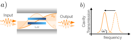
Figure 6: Figure cross-Kerr effect characterization. (a) Scheme of a setup for probing the Kerr and cross-Kerr effects. (b) Resonant driving of one of the junction eigenmodes leads to a frequency shift of another mode which can be probed by a weak laser.

References

- Devoret and Schoelkopf (2013) M. H. Devoret and R. J. Schoelkopf, Science 339, 1169 (2013).
- Houck et al. (2012) A. A. Houck, H. E. Türeci, and J. Koch, Nature Physics 8, 292 (2012).
- Carusotto et al. (2020) I. Carusotto, A. A. Houck, A. J. Kollár, P. Roushan, D. I. Schuster, and J. Simon, Nature Physics 16, 268 (2020).
- Kjaergaard et al. (2020) M. Kjaergaard, M. E. Schwartz, J. Braumüller, P. Krantz, J. I.-J. Wang, S. Gustavsson, and W. D. Oliver, Annual Review of Condensed Matter Physics 11, 369 (2020).
- Majer et al. (2007) J. Majer, J. Chow, J. Gambetta, J. Koch, B. Johnson, J. Schreier, L. Frunzio, D. Schuster, A. A. Houck, A. Wallraff, et al., Nature 449, 443 (2007).
- Blais et al. (2004) A. Blais, R.-S. Huang, A. Wallraff, S. M. Girvin, and R. J. Schoelkopf, Physical Review A 69, 062320 (2004).
- Blais et al. (2021) A. Blais, A. L. Grimsmo, S. M. Girvin, and A. Wallraff, Reviews of Modern Physics 93, 025005 (2021).
- Nigg et al. (2012) S. E. Nigg, H. Paik, B. Vlastakis, G. Kirchmair, S. Shankar, L. Frunzio, M. Devoret, R. Schoelkopf, and S. Girvin, Physical Review Letters 108, 240502 (2012).
- Minev et al. (2021) Z. K. Minev, Z. Leghtas, S. O. Mundhada, L. Christakis, I. M. Pop, and M. H. Devoret, npj Quantum Information 7, 131 (2021).
- Tinkham (2004) M. Tinkham, Introduction to superconductivity (Courier Corporation, 2004).
- Sboychakov et al. (2008) A. Sboychakov, S. Savel’ev, and F. Nori, Physical Review B 78, 134518 (2008).
- Ustinov et al. (1993) A. V. Ustinov, H. Kohlstedt, M. Cirillo, N. F. Pedersen, G. Hallmanns, and C. Heiden, Phys. Rev. B 48, 10614 (1993).
- Ustinov (1998) A. Ustinov, Physica D: Nonlinear Phenomena 123, 315 (1998).
- Kemp et al. (2002) A. Kemp, A. Wallraff, and A. V. Ustinov, physica status solidi (b) 233, 472 (2002).
- Fitzpatrick et al. (2017) M. Fitzpatrick, N. M. Sundaresan, A. C. Li, J. Koch, and A. A. Houck, Physical Review X 7, 011016 (2017).
- Kockum et al. (2014) A. F. Kockum, P. Delsing, and G. Johansson, Physical Review A 90, 013837 (2014).
- Wang et al. (2021) X. Wang, T. Liu, A. F. Kockum, H.-R. Li, and F. Nori, Physical Review Letters 126, 043602 (2021).
- Kannan et al. (2020) B. Kannan, M. J. Ruckriegel, D. L. Campbell, A. Frisk Kockum, J. Braumüller, D. K. Kim, M. Kjaergaard, P. Krantz, A. Melville, B. M. Niedzielski, et al., Nature 583, 775 (2020).
- Kivshar and Malomed (1989a) Y. S. Kivshar and B. A. Malomed, Rev. Mod. Phys. 61, 763 (1989a).
- Koch et al. (2007) J. Koch, M. Y. Terri, J. Gambetta, A. A. Houck, D. I. Schuster, J. Majer, A. Blais, M. H. Devoret, S. M. Girvin, and R. J. Schoelkopf, Physical Review A 76, 042319 (2007).
- Kakazu and Kim (1994) K. Kakazu and Y. Kim, Physical Review A 50, 1830 (1994).
- Grynberg et al. (2010) G. Grynberg, A. Aspect, and C. Fabre, Introduction to quantum optics: from the semi-classical approach to quantized light (Cambridge university press, 2010).
- Bothner et al. (2013) D. Bothner, M. Knufinke, H. Hattermann, R. Wölbing, B. Ferdinand, P. Weiss, S. Bernon, J. Fortágh, D. Koelle, and R. Kleiner, New Journal of Physics 15, 093024 (2013).
- Schmidt and Koch (2013) S. Schmidt and J. Koch, Annalen der Physik 525, 395 (2013).
- Sundaresan et al. (2019) N. M. Sundaresan, R. Lundgren, G. Zhu, A. V. Gorshkov, and A. A. Houck, Physical Review X 9, 011021 (2019).
- Mirhosseini et al. (2018) M. Mirhosseini, E. Kim, V. S. Ferreira, M. Kalaee, A. Sipahigil, A. J. Keller, and O. Painter, Nature communications 9, 3706 (2018).
- Van der Zant et al. (1992) H. Van der Zant, F. Fritschy, W. Elion, L. Geerligs, and J. Mooij, Physical review letters 69, 2971 (1992).
- Makhlin et al. (2001) Y. Makhlin, G. Schön, and A. Shnirman, Reviews of modern physics 73, 357 (2001).
- Hartmann et al. (2008) M. J. Hartmann, F. G. Brandao, and M. B. Plenio, Laser & Photonics Reviews 2, 527 (2008).
- Kleine et al. (2008) A. Kleine, C. Kollath, I. McCulloch, T. Giamarchi, and U. Schollwöck, Physical Review A 77, 013607 (2008).
- Cazalilla and Ho (2003) M. Cazalilla and A. Ho, Physical review letters 91, 150403 (2003).
- Recati et al. (2003) A. Recati, P. Fedichev, W. Zwerger, and P. Zoller, Physical review letters 90, 020401 (2003).
- Cole et al. (2012) W. S. Cole, S. Zhang, A. Paramekanti, and N. Trivedi, Physical review letters 109, 085302 (2012).
- Dhar et al. (2012) A. Dhar, M. Maji, T. Mishra, R. Pai, S. Mukerjee, and A. Paramekanti, Physical Review A 85, 041602 (2012).
- Hafezi et al. (2007) M. Hafezi, A. S. Sørensen, E. Demler, and M. D. Lukin, Physical Review A 76, 023613 (2007).
- Tokuno and Georges (2014) A. Tokuno and A. Georges, New Journal of Physics 16, 073005 (2014).
- Rossini and Fazio (2007) D. Rossini and R. Fazio, Physical Review Letters 99, 186401 (2007).
- Aidelsburger et al. (2022) M. Aidelsburger, L. Barbiero, A. Bermudez, T. Chanda, A. Dauphin, D. González-Cuadra, P. R. Grzybowski, S. Hands, F. Jendrzejewski, J. Jünemann, et al., Philosophical Transactions of the Royal Society A 380, 20210064 (2022).
- Osborne et al. (2022) J. Osborne, I. P. McCulloch, B. Yang, P. Hauke, and J. C. Halimeh, arXiv preprint ARXIV.2211.01380 (2022).
- Mil et al. (2020) A. Mil, T. V. Zache, A. Hegde, A. Xia, R. P. Bhatt, M. K. Oberthaler, P. Hauke, J. Berges, and F. Jendrzejewski, Science 367, 1128 (2020).
- Mamin et al. (2021) H. Mamin, E. Huang, S. Carnevale, C. Rettner, N. Arellano, M. Sherwood, C. Kurter, B. Trimm, M. Sandberg, R. Shelby, et al., Physical Review Applied 16, 024023 (2021).
- Poole et al. (2013) C. P. Poole, H. A. Farach, and R. J. Creswick, Superconductivity (Academic press, 2013).
- Wallraff et al. (2004) A. Wallraff, D. I. Schuster, A. Blais, L. Frunzio, R.-S. Huang, J. Majer, S. Kumar, S. M. Girvin, and R. J. Schoelkopf, Nature 431, 162 (2004).
- Wonneberger (1980) W. Wonneberger, Physica A: Statistical Mechanics and its Applications 103, 543 (1980).
- Kivshar and Malomed (1989b) Y. S. Kivshar and B. A. Malomed, Reviews of Modern Physics 61, 763 (1989b).
- Altland and Simons (2010) A. Altland and B. D. Simons, Condensed matter field theory (Cambridge university press, 2010).
- Sun et al. (2020) Z. Sun, M. Fogler, D. Basov, and A. J. Millis, Physical Review Research 2, 023413 (2020).
- Scully and Zubairy (1999) M. O. Scully and M. S. Zubairy, “Quantum optics,” (1999).