On Quaternion Higher-Order Singular Value Decomposition: Models and Analysis

Abstract

Higher-order singular value decomposition (HOSVD) is one of the most celebrated tensor decompositions that generalizes matrix SVD to higher-order tensors. It was recently extended to the quaternion domain [17] (we refer to it as L-QHOSVD in this work). However, due to the non-commutativity of quaternion multiplications, L-QHOSVD is inconsistent with matrix SVD when the order of the quaternion tensor collapses to $2$; moreover, theoretical guaranteed truncated L-QHOSVD was not investigated. The first contribution of this work is a more natural higher-order generalization of the quaternion matrix SVD. To this end, we first utilize the feature that left and right multiplications of quaternions are inconsistent to define left and right quaternion tensor unfoldings and mode-$k$ products. Then, by using these basic tools, we propose a two-sided quaternion higher-order singular value decomposition (TS-QHOSVD), which has the following two main features: 1) it computes two factor matrices at a time from SVDs of left and right unfoldings, inheriting certain parallel properties of the original HOSVD; 2) it is consistent with matrix SVD when the order of the tensor is $2$. The ordering and orthogonality properties of TS-QHOSVD are studied. Correspondingly, quaternion HOSVD based on right products (R-QHOSVD) is also briefly introduced. Our second contribution is to propose truncated versions of TS-, L-, and R-QHOSVD and establish their error bounds measured by the tail energy. What makes these results nontrivial is that the error bound analysis is quite different from their real or complex counterparts, again due to the non-commutativity of quaternion multiplications. In addition, via counterexamples, we point out that the reconstructed tensor may not be a $\sqrt{N}$-suboptimal solution, and may not be of low rank in all modes. Finally, we provide numerical examples to illustrate the derived properties of TS-QHOSVD and the efficacy of truncated QHOSVDs.

Key words: Tensor, quaternion tensors, quaternion tensor unfolding, higher-order singular value decomposition, error bound

AMS subject classifications. 11R52, 15A69, 15A72, 65F99

1 Introduction

Tensor decomposition and approximation have become more and more important in the big-data era. Encoding multi-dimensional and multi-modal data into a tensor-based format allows us to exploit fully their inherent features. Many different tensor decompositions have been proposed to facilitate analysis and compression of tensor data. The most common ones are the canonical polyadic decomposition, Tucker decomposition [14], block term decomposition [4], tensor ring [31], tensor-train [21], and tensor SVD [13]; see also the nice surveys in tensor decompositions and applications [3, 2, 14, 25]. The celebrated multilinear singular value decomposition [5] (HOSVD) is a special case of Tucker decomposition that factorizes the unfolding matrices of the data tensor along each mode independently using matrix SVD. To speed up HOSVD, the sequential HOSVD was proposed in [26], which generates factor matrices sequentially from a tensor that is given by the products of the data tensor and the previously computed factor matrices–a tensor with possible a smaller and smaller size.

Quaternions generalize complex numbers to four dimensions. A main difference between quaternions and the real or complex numbers is that quaternion multiplication is non-commutative, i.e., $pq\neq qp$ for general quaternions $p,q$. As will be seen in this work, such a property causes several troubles. Nevertheless, owing to its ability to represent 3D and 4D vectors as single quaternion scalars, the study of quaternions has become more and more popular, especially in image and video processing, such as image fusion and denoising [17], face recognition [33, 34], color video approximation [18, 23, 16], and inpainting [11, 15, 8, 1]. Quaternion matrix optimization also draws much attention [28, 29, 22]. A very recent comprehensive survey of applications in signal and image processing can be referred to [20]. The success of quaternions in applications lies in the successful generalization of several matrix decompositions and computations to the quaternion domain [30, 24, 27, 12, 10, 9], albeit its non-commutativity. As a color video can be represented by a third-order quaternion tensor, many tensor algebras have also been studied and extended to the quaternion case. Examples include QT-product [23, 16, 32], quaternion tensor-train decomposition [19], quaternion mode-$k$ product [18, 17], and Einstein product [6]. Based on the left and right products of quaternions, possible extensions of Tucker decomposition and CP decomposition to the quaternion domain were studied [7]; it should be noted that the left and right products defined in [7] are different from those to be defined in this work, which will be compared later.

In [17], Miao et al. extended the sequential HOSVD [26] to the quaternion domain. They proved the existence of such a decomposition and the ordering property of subtensors of the core tensor. The authors then applied the quaternion HOSVD to color image fusion and denoising. Essentially, their quaternion HOSVD is based on left multiplications (and due to this reason, we term it as L-QHOSVD), namely, the quaternion data tensor is decomposed as a core tensor left multiplied by factor matrices along each mode, where the factor matrices are computed sequentially. However, unlike the real or complex cases, quaternion tensor-matrix products have some ambiguities in that left and right quaternion products are inconsistent, due to that quaternion multiplications are non-commutative. As a consequence, L-QHOSVD may not consistent with quaternion matrix SVD when the order of the tensor is $2$; this will be proved in Sect. 4.

In practice, an approximation instead of an exact decomposition may be more preferred for dimension reduction, data compression, or denoising, because the real-world data may approximately lie in a low-dimensional subspace. To this end, truncated tensor decomposition models are important. Truncated HOSVDs [5, 26] discard the entries of the core tensor and columns of factor matrices corresponding to the discarded singular values, where the error is bounded by the tail energy, namely, the sum of squares of the discarded singular values. Alternatively, [17] truncated the core tensor using hard thresholding. Although [17] showed that this strategy also performs well in image denoising, it seems hard to establish a theoretical error bound and estimate the compressed ratio for this type of truncation.

In view of the above understandings of L-QHOSVD, the first contribution in this work is an alternative version of quaternion HOSVD. Our starting point still mainly follows the sequential HOSVD [26]. However, by taking account of the non-commutativity of multiplications of quaternions, at each round of the computation, we prefer to compute two factor matrices (simultaneously) from the SVDs of what we call the left and right unfoldings of the tensor, respectively. Therefore, our HOSVD inherits part of the parallel property of the original HOSVD [5]. This is also an advantage over L-QHOSVD. For preparing the next round of computation, the tensor is then multiplied from left and right by the two computed factor matrices, respectively. Since our HOSVD computes factor matrices from both sides, we call it two-sided quaternion HOSVD (TS-QHOSVD). TS-QHOSVD is a more natural generalization of the matrix SVD, as it is consistent with SVD when the order of the tensor collapses to $2$. We show that the core tensor also admits the ordering and orthogonality properties; in particular, the orthogonality only holds at the first and the last modes, while for all modes, weak orthogonality still holds–the latter was not investigated in L-QHOSVD. Correspondingly, we also briefly introduce the QHOSVD based on right products (R-QHOSVD) and its properties.

Our second contribution is the truncated TS-QHOSVD (and also L-QHOSVD and R-QHOSVD) and its error bound analysis. Following the line of truncated HOSVDs [5, 26], we propose the truncated QHOSVDs by truncating the subspaces corresponding to the discarded singular values. Similar error bounds measured by the tail energy as those in [5, 26] are established. However, establishing the error bound is quite nontrivial: in the real or complex cases, key to the error analysis is that the reconstructed tensor can be expressed as

$$\hat{\mathcal{T}}=\mathcal{T}\times_{1}(\hat{\mathbf{U}}_{1}\hat{\mathbf{U}}_{1}^{H})\cdots\times_{N}(\hat{\mathbf{U}}_{N}\hat{\mathbf{U}}_{N}^{H}),$$

which is the multi-projection of the original data tensor onto multilinear subspaces spanned by the non-discarded singular vectors. While, due to the non-commutativity, such a nice structure is no longer valid in the quaternion domain, resulting in a different analysis; see the analysis in Sect. 5. In addition, via counterexamples, we point out that the reconstructed tensor may not be a $\sqrt{N}$-suboptimal solution, and may not be of low rank in all modes. These two points are quite different from their real or complex counterparts.

In summary, our contributions in this work are mainly on new models and their theoretical analysis: the TS-QHOSVD and its properties; the truncated TS-, L-, and R-QHOSVD and their error bounds analysis, along with some new notions of unfolding and tensor-matrix products.

The rest is organized as follows. Sect. 2 prepares notations and preliminaries on quaternion algebra. In Sect. 3, we introduce necessary computations concerning quaternion tensors, including left and right mode-$k$ unfolding, left and right mode-$k$ products, and some properties. Sect. 4 presents TS-QHOSVD and its properties; correspondingly, L-QHOSVD and R-QHOSVD are also discussed. Then, the truncated QHOSVDs with their error bounds are investigated in Sect. 5. Numerical examples are provided in Sect. 6. Finally, some conclusions are drawn in Sect. 7.

2 Preliminaries

Notations

$\mathbb{R},\mathbb{C}$ and $\mathbb{H}$ respectively denote the real, complex, and quaternion space. $\mathbb{H}^{I_{1}\times I_{2}\times\cdots\times I_{N}}$ represents the $N$-th order quaternion tensor space. A scalar, vector, matrix, and tensor are written as $a$, $\mathbf{a}$, $\mathbf{A}$, and $\mathcal{A}$, respectively. $\bar{(\cdot)}$, $(\cdot)^{T}$, and $(\cdot)^{H}$ respectively represent the conjugate, transpose, and conjugate transpose. $\|\cdot\|_{F}$ is the Frobenius norm. $\otimes$ denotes the Kronecker product. $tr(\cdot)$ represents the trace of a matrix.

We remark that in this work, the $(i,j)$-th entry of a matrix $\mathbf{A}$ is written as $a_{ij}$, and the $(i_{1},\ldots,i_{N})$-th entry of a tensor $\mathcal{A}$ is written as $a_{i_{1}\cdots i_{N}}$. However, in some contexts, it is more convenient to use the MATLAB notations $\mathbf{A}(i,j)$ and $\mathcal{A}(i_{1},\ldots,I_{N})$ to denote the same entries. Correspondingly, the MATLAB notations $\mathbf{A}(i,:)$ and $\mathbf{A}(:,j)$ respectively represent the $i$-th row and the $j$-th column of $\mathbf{A}$.

A four-dimensional non-commutative division algebra $\mathbb{H}$ is defined over the real numbers $\mathbb{R}$ with canonical basis $\{1,\bf i,j,k\}$. Here ${\bf i},{\bf j},{\bf k}$ are imaginary units satisfying

$$\bf{i}^{2}=\bf{j}^{2}=\bf{k}^{2}={\bf ijk}=-1$$

and

$$\bf{ij}=-\bf{ji}=k,\bf{jk}=-\bf{kj}=\bf{i},\bf{ki}=-\bf{ik}=\bf{j}.$$

Any quaternion $q\in\mathbb{H}$ can be written as

$$q=q_{0}+q_{1}{\bf i}+{q_{2}}{\bf j}+q_{3}{\bf k},$$

where $q_{0},q_{1},q_{2},q_{3}\in\mathbb{R}$ are the components of $q$. The real and imaginary parts of $q$ are denoted as $Re(q)=q_{0}$ and $Im(q)=q_{1}{\bf i}+q_{2}{\bf j}+q_{3}{\bf k}$ respectively. Non-commutativity of quaternion multiplications implies that for any $p,q\in\mathbb{H}$, one has $pq\neq qp$ in general. $\bar{q}=q_{0}-q_{1}{\bf i}-q_{2}{\bf j}-q_{3}{\bf k}$ is denoted as the quaternion conjugate of $q$, and it holds that $\overline{pq}=\overline{qp}$. For $q\in\mathbb{H}$, its modulus is defined as $|q|=\sqrt{q\bar{q}}=\sqrt{\bar{q}q}=\sqrt{q_{0}^{2}+q_{1}^{2}+q_{2}^{2}+q_{3}^{2}}.$

Proposition 2.1 (c.f. [30]).

For given two quaternion matrices $\mathbf{P}\in\mathbb{H}^{M\times N}$ and $\mathbf{Q}\in\mathbb{H}^{N\times M}$.Then

• $(\mathbf{P}\mathbf{Q})^{H}=\mathbf{Q}^{H}\mathbf{P}^{H}$; $(\mathbf{P}\mathbf{Q})^{T}\neq\mathbf{Q}^{T}\mathbf{P}^{T}$ in general; $\overline{\mathbf{P}\mathbf{Q}}\neq\bar{\mathbf{P}}\bar{\mathbf{Q}}$ in general.

Although $(\mathbf{P}\mathbf{Q})^{T}\neq\mathbf{Q}^{T}\mathbf{P}^{T}$ for two general quaternion matrices, if one of them is real, then as real numbers and quaternions commute, this relation is still valid:

Proposition 2.2.

Assume that $\mathbf{P}\in\mathbb{R}^{M\times N}$ and $\mathbf{Q}\in\mathbb{H}^{N\times M}$, or $\mathbf{P}\in\mathbb{H}^{M\times N}$ and $\mathbf{Q}\in\mathbb{R}^{N\times M}$. Then $(\mathbf{P}\mathbf{Q})^{T}=\mathbf{Q}^{T}\mathbf{P}^{T}$.

It is also easy to see that:

Proposition 2.3.

For any $\mathbf{A}\in\mathbb{H}^{M\times N}$ and $\mathbf{B}\in\mathbb{H}^{N\times M}$, we have $Re(\mathbf{A}\mathbf{B})=Re(\bar{\mathbf{A}}\bar{\mathbf{B}})$.

For unitary matrices, it is not difficult to verify the following:

Proposition 2.4.

Let $\mathbf{U},\mathbf{V}$ be two unitary quaternion matrices. Then their Kronecker product $\mathbf{U}\otimes\mathbf{V}$ is still unitary.

Unlike the real or complex cases, if $\mathbf{U}$ is a unitary quaternion matrix, then its transpose $\mathbf{U}^{T}$ may not be. Such a phenomenon causes troubles in the analysis in Sect. 4 and 5.

Singular value decomposition of a quaternion matrix is also valid:

Theorem 2.1 (Quaternion SVD [30]).

Let $\mathbf{T}\in\mathbb{H}^{I_{1}\times I_{2}}$ be of rank $r$. Then, there exist two unitary quaternion matrices $\mathbf{U}\in\mathbb{H}^{I_{1}\times I_{1}}$ and $\mathbf{V}\in\mathbb{H}^{I_{2}\times I_{2}}$ such that

$$\mathbf{U}^{H}\mathbf{T}\mathbf{V}=\Sigma=\begin{bmatrix}\Sigma_{r}&0\\ 0&0\end{bmatrix}.$$

where $\Sigma_{r}=diag(\sigma_{1},\dots,\sigma_{r})$ is a real diagonal matrix with $r$ positive entries $\sigma_{k}$, $(k=1,\dots,r)$ on its diagonal, which are positive singular values of the quaternion matrix $\mathbf{T}$.

Quaternion tensors are defined as follows.

Definition 2.1 (Quaternion tensors).

An $N$-th order tensor is called a quaternion tensor if its entries are quaternions, i.e.,

$$\mathcal{T}=(t_{i_{1}i_{2}\cdots i_{N}})\in\mathbb{H}^{I_{1}\times I_{2}\times\cdots\times I_{N}}=\mathcal{T}_{0}+\mathcal{T}_{1}\bf{i}+\mathcal{T}_{2}\bf{j}+\mathcal{T}_{3}\bf{k}$$

with $\mathcal{T}_{i}\in\mathbb{R}^{I_{1}\times I_{2}\times\cdots\times I_{N}},i=0,\ldots,3$. $\mathcal{T}$ is a pure tensor if $\mathcal{T}_{0}$ is zero.

We present the definitions of inner product, orthogonality, and Frobenius norm for quaternion tensors.

Definition 2.2 (Inner product).

The left and right inner products of two quaternion tensors $\mathcal{A},\mathcal{B}\in\mathbb{H}^{I_{1}\times I_{2}\times\cdots\times I_{N}}$ are respectively defined as

$$\begin{split}&\langle\mathcal{A},\mathcal{B}\rangle_{L}=\sum_{i_{1}=1}^{I_{1}}\sum_{i_{2}=1}^{I_{2}}\cdots\sum_{i_{N}=1}^{I_{N}}a_{i_{1}i_{2}\cdots i_{N}}\bar{b}_{i_{1}i_{2}\cdots i_{N}};\\ &\langle\mathcal{A},\mathcal{B}\rangle_{R}=\sum_{i_{1}=1}^{I_{1}}\sum_{i_{2}=1}^{I_{2}}\cdots\sum_{i_{N}=1}^{I_{N}}\bar{a}_{i_{1}i_{2}\cdots i_{N}}b_{i_{1}i_{2}\cdots i_{N}}.\end{split}$$

Here, the right inner product coincides with the (standard) quaternion matrix inner product; see, e.g., [1, 22], and its conjugation coincides with the quaternion vector inner product [24]. On the other hand, it is easy to see that $\widebar{\langle\mathcal{A},\mathcal{B}\rangle_{L}}=\langle\mathcal{B},\mathcal{A}\rangle_{L}$ and $\widebar{\langle\mathcal{A},\mathcal{B}\rangle_{R}}=\langle\mathcal{B},\mathcal{A}\rangle_{R}$.

Definition 2.3 (Orthogonality).

For $\mathcal{A},\mathcal{B}\in\mathbb{H}^{I_{1}\times I_{2}\times\cdots\times I_{N}}$, if $\langle\mathcal{A},\mathcal{B}\rangle_{L}=0$, then we say that they are left orthogonal; if $\langle\mathcal{A},\mathcal{B}\rangle_{R}=0$, then we say that they are right orthogonal; if $Re\langle\mathcal{A},\mathcal{B}\rangle_{L}=Re\langle\mathcal{A},\mathcal{B}\rangle_{R}=0$, then we say that they are weakly orthogonal.

The right orthogonality coincides with the notion of orthogonality of two quaternion vectors [24]. On the other hand, one always has for any $\mathcal{A},\mathcal{B}$ of the same order, $Re\langle\mathcal{A},\mathcal{B}\rangle_{L}=Re\langle\mathcal{A},\mathcal{B}\rangle_{R}=Re\langle\mathcal{B},\mathcal{A}\rangle_{L}=Re\langle\mathcal{B},\mathcal{A}\rangle_{R}$.

The Frobenius norm of quaternion tensors is given by

$$\|\mathcal{A}\|_{F}^{2}=\langle\mathcal{A},\mathcal{A}\rangle_{L}=\langle\mathcal{A},\mathcal{A}\rangle_{R}.$$

3 Left and Right Computations

In this section, we introduce left/right mode-$k$ unfoldings, left/right mode-$k$ products, and their necessary properties for later use.

3.1 Left and right mode-$k$ unfoldings

Definition 3.1 (Left mode-$k$ unfolding).

For an $N$-th order quaternion tensor $\mathcal{T}\in\mathbb{H}^{I_{1}\times I_{2}\times\cdots\times I_{N}}$, its left mode-$k$ unfolding is denoted as $\mathbf{T}^{L}_{[k]}$ and arranges the mode-$k$ fibers to the columns of the resulting quaternion matrix, i.e.,

$$\mathbf{T}^{L}_{[k]}\in\mathbb{H}^{I_{k}\times I_{1}\cdots I_{k-1}I_{k+1}\cdots I_{N}}.$$

The $(i_{1},i_{2},\dots,i_{N})$-th entry of $\mathcal{T}$ maps to the $(i_{k},j)$-th entry of $\mathbf{T}^{L}_{[k]}$, where

$$j=1+\sum_{\begin{subarray}{c}l=1\\ l\neq k\end{subarray}}^{N}\nolimits(i_{l}-1)J_{l}\qquad\text{with}\qquad J_{l}=\prod\nolimits_{\begin{subarray}{c}m=1\\ m\neq k\end{subarray}}^{l-1}I_{m}.$$

The above definition is analogous to the real or complex tensor unfoldings [14]. In the quaternion case, it was first given in [18] without the adjective “left”. We call it left unfolding to distinguish it from the right unfolding to be defined immediately:

Definition 3.2 (Right mode-$k$ unfolding).

For an $N$-th order quaternion tensor $\mathcal{T}\in\mathbb{H}^{I_{1}\times I_{2}\times\cdots\times I_{N}}$, its right mode-$k$ unfolding is denoted as $\mathbf{T}^{R}_{[k]}$ and arranges the mode-$k$ fibers to be the rows of the quaternion matrix, i.e.,

$$\mathbf{T}^{R}_{[k]}\in\mathbb{H}^{I_{1}\cdots I_{k-1}I_{k+1}\cdots I_{N}\times I_{k}}.$$

The $(i_{1},i_{2},\dots,i_{N})$-th entry of $\mathcal{T}$ maps to the $(j,i_{k})$-th entry of $\mathbf{T}^{R}_{[k]}$, where

$$j=1+\sum_{\begin{subarray}{c}l=1\\ l\neq k\end{subarray}}^{N}\nolimits(i_{l}-1)J_{l}\qquad\text{with}\qquad J_{l}=\prod\nolimits_{\begin{subarray}{c}m=1\\ m\neq k\end{subarray}}^{l-1}I_{m}.$$

Although it holds that $\mathbf{T}^{L}_{[k]}=(\mathbf{T}^{R}_{[k]})^{T}$, it is convenient to distinguish left and right unfoldings in our later analysis.

3.2 Left and right mode-$k$ products

Recall that for a real tensor $\mathcal{T}\in\mathbb{R}^{I_{1}\times\cdots\times I_{N}}$ and a real matrix $\mathbf{U}\in\mathbb{R}^{J\times I_{k}}$, the mode-$k$ product of $\mathcal{T}$ and $\mathbf{U}$ is given by $\mathcal{Y}=\mathcal{T}\times_{k}\mathbf{U}$, with entries

$$y_{i_{1}\cdots i_{k-1}ji_{k+1}\cdots i_{N}}=\sum_{i_{k}=1}^{I_{k}}t_{i_{1}i_{2}\cdots i_{N}}u_{ji_{k}}=\sum_{i_{k}=1}^{I_{k}}u_{ji_{k}}t_{i_{1}i_{2}\cdots i_{N}}.$$

The second equation holds because of the commutativity of real multiplications. However, things change if $\mathcal{T}$ and $\mathbf{U}$ are both quaternions: due to the non-commutativity, in general

$$\sum_{i_{k}=1}^{I_{k}}t_{i_{1}i_{2}\dots i_{N}}u_{ji_{k}}\neq\sum_{i_{k}=1}^{I_{k}}u_{ji_{k}}t_{i_{1}i_{2}\cdots i_{N}}.$$

Therefore, this leads to an ambiguity: When we talk about quaternion tensor-matrix products, which definition should we use?

To resolve this problem, it is natural to define left and right mode-$k$ products respectively, depending on the multiplication of the matrix from left or right.

Definition 3.3 (Left mode-$k$ product).

The left mode-$k$ product of a quaternion tensor $\mathcal{T}\in\mathbb{H}^{I_{1}\times I_{2}\times\cdots\times I_{N}}$ with a quaternion matrix $\mathbf{U}\in\mathbb{H}^{J\times I_{k}}$ is denoted as

$$\mathcal{Y}=\mathbf{U}\times_{k}^{L}\mathcal{T}\in\mathbb{H}^{I_{1}\times\cdots\times I_{k-1}\times J\times I_{k+1}\times\cdots\times I_{N}}$$

with entries

$$y_{i_{1}\cdots n_{k-1}jn_{k+1}\cdots i_{N}}=\sum_{i_{k}=1}^{I_{k}}u_{ji_{k}}t_{i_{1}i_{2}\cdots i_{N}}.$$

Definition 3.4 (Right mode-$k$ product).

The right mode-$k$ product of a quaternion tensor $\mathcal{T}\in\mathbb{H}^{I_{1}\times I_{2}\times\cdots\times I_{N}}$ with a quaternion matrix $\mathbf{V}\in\mathbb{H}^{I_{k}\times J}$ is denoted as

$$\mathcal{Y}=\mathcal{T}\times_{k}^{R}\mathbf{V}\in\mathbb{H}^{I_{1}\times\cdots\times I_{k-1}\times J\times I_{k+1}\times\cdots\times I_{N}}$$

with entries

$$y_{i_{1}\cdots i_{k-1}ji_{k+1}\cdots i_{N}}=\sum_{i_{k}=1}^{I_{k}}t_{i_{1}i_{2}\cdots i_{N}}v_{i_{k}j}.$$

Note that different from the mode-$k$ product in the real case, the above definition sums the entries of $t_{i_{1}i_{2}\cdots i_{N}}v_{i_{k}j}$ by running over all the row indices of $v_{i_{k}j}$ instead of its column indices.

Some more remarks of left and right mode-$k$ products are in order.

Remark 1.

1. Left and right mode-$k$ products are natural generalizations of matrix products: Given $\mathbf{U}\in\mathbb{H}^{I\times J},\mathbf{S}\in\mathbb{H}^{J\times K},\mathbf{V}\in\mathbb{H}^{K\times L}$, one has

$$\mathbf{U}\times_{1}^{L}\mathbf{S}\times_{2}^{R}\mathbf{V}=\mathbf{U}\mathbf{S}\mathbf{V}.$$

2. The left mode-$k$ product was defined in [19] without the adjective “left” ([19] used the conventional notation $\times_{k}$ instead of $\times^{L}_{k}$).

3. [7] also introduced the notions of left and right mode-$k$ products very recently. Specifically, the authors of [7] defined three types of products:

• left mode-$1$ product: $\left(\mathcal{T}\times_{1}^{L}\mathbf{U}\right)_{ji_{2}\cdots i_{N}}=\sum^{I_{1}}_{i_{1}=1}u_{ji_{1}}t_{i_{1}i_{2}\cdots i_{N}}$ for $\mathbf{U}\in\mathbb{H}^{J\times I_{1}}$;

• right mode-$N$ product: $\left(\mathcal{T}\times_{N}^{R}\mathbf{U}\right)_{i_{1}\cdots i_{N-1}j}=\sum^{I_{N}}_{i_{N}=1}t_{i_{1}\cdots i_{N}}u_{ji_{N}}$ for $\mathbf{U}\in\mathbb{H}^{J\times I_{N}}$;

• mode-$d$ ($2\leq d\leq N-1$) product of a real matrix: $\left(\mathcal{T}\times_{d}\mathbf{U}\right)_{i_{1}\cdots j\cdots i_{N}}=\sum^{I_{d}}_{i_{d}=1}t_{i_{1}\cdots i_{d}\cdots i_{N}}u_{ji_{d}}$ for $U\in\mathbb{R}^{J\times I_{d}}$.

Comparing our definitions of left and right products with those in [7], we can see that they are quite different:

• the left product of [7] is only defined for mode-$1$, while ours can be for any mode;

• the right product of [7] is only defined for mode-$N$, while ours can be for any mode;

• for mode-$d$ $(2\leq d\leq N-1)$ products, [7] requires a real matrix $\mathbf{U}$, while ours can be quaternion; this point is the main difference;

• For mode-$d$ $(2\leq d\leq N)$ product, [7] sums the entries by running over the column indices of $U$, while ours runs over its row indices.

Therefore, our definitions are more flexible and general.

The following basic properties of left products were summarized in [19]:

Lemma 3.1.

1. Left mode-$k$ product can be expressed in terms of its left unfolding:

   $$\mathcal{Y}=\mathbf{U}\times_{k}^{L}\mathcal{T}\Leftrightarrow\mathbf{Y}_{[k]}^{L}=\mathbf{U}\mathbf{T}_{[k]}^{L}.$$

2. Left multiplied several quaternion matrices of proper sizes on the same mode of a quaternion tensor is given by

   $$\mathbf{U}_{2}\times_{k}^{L}\mathbf{U}_{1}\times_{k}^{L}\mathcal{T}=(\mathbf{U}_{2}\mathbf{U}_{1})\times_{k}^{L}\mathcal{T}.$$

3. If a quaternion tensor is multiplied by several quaternion matrices on different modes, then the order of the multiplications is vitally important, i.e., if $k_{1}\neq k_{2}$, in general

   $$\mathbf{U}_{k_{2}}\times_{k_{2}}^{L}\mathbf{U}_{k_{1}}\times_{k_{1}}^{L}\mathcal{T}\neq\mathbf{U}_{k_{1}}\times_{k_{1}}^{L}\mathbf{U}_{k_{2}}\times_{k_{2}}^{L}\mathcal{T}.$$

Correspondingly, right products admit similar properties, which can be checked directly and the proof is omitted.

Lemma 3.2.

1. Right mode-$k$ product can be expressed in terms of its right unfolding:

   $$\mathcal{Y}=\mathcal{T}\times_{k}^{R}\mathbf{V}\Leftrightarrow\mathbf{Y}^{R}_{[k]}=\mathbf{T}_{[k]}^{R}\mathbf{V}.$$

2. Right multiplied several quaternion matrices of proper sizes on the same mode of a quaternion tensor is given by

   $$\mathcal{T}\times_{k}^{R}\mathbf{V}_{1}\times_{k}^{R}\mathbf{V}_{2}=\mathcal{T}\times_{k}^{R}(\mathbf{V}_{1}\mathbf{V}_{2}).$$

3. If a quaternion tensor is multiplied by several quaternion matrices on different modes, then the order of the multiplications is vitally important, i.e., if $k_{1}\neq k_{2}$, in general

   $$\mathcal{T}\times_{k_{1}}^{R}\mathbf{V}_{k_{1}}\times_{k_{2}}^{R}\mathbf{V}_{k_{2}}\neq\mathcal{T}\times_{k_{2}}^{R}\mathbf{V}_{k_{2}}\times_{k_{1}}^{R}\mathbf{V}_{k_{1}}.$$

Remark 2.

In the real or complex cases, one has

$$\mathcal{T}\times_{k_{1}}\mathbf{U}_{k_{1}}\times_{k_{2}}\mathbf{U}_{k_{2}}=\mathcal{T}\times_{k_{2}}\mathbf{U}_{k_{2}}\times_{k_{1}}\mathbf{U}_{k_{1}},$$ (3.1)

i.e., the order of the multiplications can be arbitrarily changed, provided that $k_{1}\neq k_{2}$. Losing this property prevents the construction of products of projection matrices when analyzing the error bounds of TS-QHOSVD (which is important for the analysis in the real case), as will be seen later in Sect. 5.

Somewhat fortunately, if considering left and right products together, the order of the multiplications can be changed, thanks to the associative law of quaternions:

Lemma 3.3.

Let $\mathcal{T}\in\mathbb{H}^{I_{1}\times I_{2}\times\cdots\times I_{N}}$, $\mathbf{U}_{k_{1}}\in\mathbb{H}^{I_{k_{1}}\times J_{k_{1}}}$, and $\mathbf{V}_{k_{2}}\in\mathbb{H}^{J_{k_{2}}\times I_{k_{2}}}$, where $k_{1}\neq k_{2}$. The following property is satisfied:

$$\mathbf{U}_{k_{1}}\times_{k_{1}}^{L}(\mathcal{T}\times_{k_{2}}^{R}\mathbf{V}_{k_{2}})=(\mathbf{U}_{k_{1}}\times_{k_{1}}^{L}\mathcal{T})\times_{k_{2}}^{R}\mathbf{V}_{k_{2}}.$$

Before ending this section, we present two lemmas conerning unfoldings of mode-$k$ products by means of the Kronecker product, whose proof will be given in Sect. A.

Lemma 3.4.

If $\mathcal{Y}=\mathbf{U}_{k}\times^{L}_{k}\mathbf{U}_{k-1}\times^{L}_{k-1}\cdots\mathbf{U}_{1}\times^{L}_{1}\mathcal{T}$, where $N>k$, then for any $N\geq j>k$ we have

$$\mathbf{Y}^{L}_{[j]}=\left((\mathbf{I}_{N}\otimes\cdots\otimes\mathbf{I}_{j+1}\otimes\mathbf{I}_{j-1}\otimes\cdots\otimes\mathbf{I}_{k+1}\otimes\mathbf{U}_{k}\otimes\cdots\otimes\mathbf{U}_{1})(\mathbf{T}^{L}_{[j]})^{T}\right)^{T}.$$

Specifically, when $j=k$ we have

$$\mathbf{Y}^{L}_{[j]}=\mathbf{U}_{j}\left((\mathbf{I}_{N}\otimes\cdots\otimes\mathbf{I}_{j+1}\otimes\mathbf{U}_{j-1}\otimes\cdots\otimes\mathbf{U}_{1})(\mathbf{T}^{L}_{[j]})^{T}\right)^{T}.$$

More generally, if $\mathcal{Y}=\mathbf{U}_{i_{k}}\times^{L}_{i_{k}}\mathbf{U}_{i_{k-1}}\times^{L}_{i_{k-1}}\cdots\mathbf{U}_{i_{1}}\times^{L}_{i_{1}}\mathcal{T}$, where $N>i_{k}>i_{k-1}>\cdots>i_{1}$, then for any $N\geq j>i_{k}$ we have

$$\mathbf{Y}^{R}_{[j]}=\left(\mathbf{H}(\mathbf{T}^{L}_{[j]})^{T}\right)^{T},$$

where

$$\mathbf{H}=\mathbf{I}_{N}\otimes\cdots\otimes\mathbf{I}_{j+1}\otimes\mathbf{I}_{j-1}\otimes\cdots\otimes\mathbf{I}_{i_{k}+1}\otimes\mathbf{U}_{i_{k}}\otimes\mathbf{I}_{i_{k}-1}\otimes\cdots\\ \otimes\mathbf{I}_{i_{k-1}+1}\otimes\mathbf{U}_{i_{k-1}}\otimes\mathbf{I}_{i_{k-1}-1}\otimes\cdots\otimes\mathbf{I}_{i_{1}+1}\otimes\mathbf{U}_{i_{1}}\otimes\mathbf{I}_{i_{1}-1}\otimes\cdots\otimes\mathbf{I}_{1}.$$

Lemma 3.5.

If $\mathcal{Y}=\mathcal{T}\times^{R}_{N}\mathbf{V}_{N}\cdots\times^{R}_{k}\mathbf{V}_{k}$, where $k>1$ then for any $k>j\geq 1$ we have

$$\mathbf{Y}^{R}_{[j]}=\left((\mathbf{T}^{R}_{[j]})^{T}(\mathbf{V}_{N}\otimes\cdots\otimes\mathbf{V}_{k}\otimes\mathbf{I}_{k-1}\otimes\cdots\otimes\mathbf{I}_{j+1}\otimes\mathbf{I}_{j-1}\otimes\cdots\otimes\mathbf{I}_{1})\right)^{T}.$$

Specifically, when $j=k$ we have

$$\mathbf{Y}^{R}_{[j]}=\left((\mathbf{T}^{R}_{[j]})^{T}(\mathbf{V}_{N}\otimes\cdots\otimes\mathbf{V}_{j+1}\otimes\mathbf{I}_{j-1}\otimes\cdots\otimes\mathbf{I}_{1})\right)^{T}\mathbf{V}_{j}.$$

More generally, if $\mathcal{Y}=\mathcal{T}\times^{R}_{i_{k}}\mathbf{V}_{i_{k}}\cdots\times^{R}_{i_{1}}\mathbf{V}_{i_{1}}$, where $i_{k}>i_{k-1}>\cdots>i_{1}>1$, then for any $i_{1}>j\geq 1$ we have

$$\mathbf{Y}^{L}_{[j]}=\left((\mathbf{T}^{R}_{[j]})^{T}\mathbf{H}\right)^{T},$$

where

$$\mathbf{H}=\mathbf{I}_{N}\otimes\cdots\otimes\mathbf{I}_{i_{k}+1}\otimes\mathbf{V}_{i_{k}}\otimes\mathbf{I}_{i_{k}-1}\otimes\cdots\otimes\mathbf{I}_{i_{k-1}+1}\otimes\mathbf{V}_{i_{k-1}}\otimes\mathbf{I}_{i_{k-1}-1}\otimes\cdots\\ \otimes\mathbf{I}_{i_{1}+1}\otimes\mathbf{V}_{i_{1}}\otimes\mathbf{I}_{i_{1}-1}\otimes\cdots\otimes\mathbf{I}_{j+1}\otimes\mathbf{I}_{j-1}\otimes\cdots\otimes\mathbf{I}_{1}.$$

4 Two-Sided Quaternion Higher-Order Singular Value Decomposition

In this section, we first recall the quaternion HOSVD proposed in [17] (L-QHOSVD). Then, to obtain a more natural generalization of the quaternion matrix SVD, we propose our TS-QHOSVD based on both left and right multiplications. Finally, quaternion HOSVD based on right multiplications (R-QHOSVD) will also be briefly introduced.

4.1 L-QHOSVD

According to [17], given $\mathcal{T}\in\mathbb{H}^{I_{1}\times\cdots\times I_{N}}$, for $k=N:-1:1$, L-QHOSVD computes the factor matrix $\mathbf{U}_{k}\in\mathbb{H}^{I_{k}\times I_{k}}$ from the left singular vector matrix of the SVD of $(\mathbf{T}_{k+1})_{[k]}^{L}$, which is the left mode-$k$ unfolding of $\mathcal{T}_{k+1}$, where the tensors $\mathcal{T}_{k}$’s are defined recursively as $\mathcal{T}_{k}:=\mathbf{U}_{k}^{H}\times_{k}^{L}\mathcal{T}_{k+1}$ with $\mathcal{T}_{N+1}:=\mathcal{T}$. Finally, the core tensor $\mathcal{S}=\mathcal{T}_{1}$.

Theorem 4.1 (L-QHOSVD [17]).

Let $\mathcal{T}\in\mathbb{H}^{I_{1}\times I_{2}\times\cdots\times I_{N}}$ be an $N$-th order quaternion tensor and let the unitary matrices $\mathbf{U}_{k}\in\mathbb{H}^{I_{k}\times I_{k}}$ ($k=N:-1:1$) and $\mathcal{S}$ be generated as above. Then, $\mathcal{T}$ can be decomposed as

$$\mathcal{T}=\mathbf{U}_{N}\times_{N}^{L}\dots\mathbf{U}_{2}\times_{2}^{L}\mathbf{U}_{1}\times_{1}^{L}\mathcal{S},$$ (4.1)

which we refer to as the left quaternion higher-order singular value decomposition (L-QHOSVD) of $\mathcal{T}$. $\mathcal{S}\in\mathbb{H}^{I_{1}\times I_{2}\times\cdots\times I_{N}}$ admits the following properties:

1. Ordering:

   $$\|\mathcal{S}_{i_{k}=1}\|_{F}=(\sigma_{1}^{L})^{(k)}\geq\|\mathcal{S}_{i_{k}=2}\|_{F}=(\sigma_{2}^{L})^{(k)}\geq\cdots\geq\|\mathcal{S}_{i_{k}=I_{k}}\|_{F}=(\sigma_{I_{k}}^{L})^{(k)}\geq 0$$

   for any $k=1,2,\dots,N$, where $\mathcal{S}_{i_{k}=\alpha}$ is the $(N-1)$-th order tensor obtained by fixing the $k$-th index of $\mathcal{S}$ to be $\alpha$, and $(\sigma_{i}^{L})^{(k)}$’s are the singular values of $(\mathbf{T}_{k+1})^{L}_{[k]}$, arranged in a descending order.

2. Orthogonality: The left orthogonality is satisfied only in mode-$1$, i.e.

   $$\langle\mathcal{S}_{i_{1}=\alpha},\mathcal{S}_{i_{1}=\beta}\rangle_{L}=0\quad\text{when}\quad\alpha\neq\beta.$$

Remark 3.

1. Essentially, the strategy of computing the factor matrices of L-QHOSVD coincides with that of the sequential HOSVD [26], i.e., the factor matrices are computed sequentially, where the current factor matrix is generated from the data tensor left multiplied by previously computed factor matrices.

2. The order of generating $\mathbf{U}_{i}$’s is arbitrary, where Theorem 4.1 takes $k=N:-1:1$ as an example. However, to recover $\mathcal{T}$, the multiplications must be in a reverse order, namely, $k=1:N$. This is because

$$\mathbf{U}_{N}\times_{N}^{L}\dots\mathbf{U}_{2}\times_{2}^{L}\mathbf{U}_{1}\times_{1}^{L}\mathcal{S}$$

$$= \mathbf{U}_{N}\times_{N}^{L}\dots\mathbf{U}_{2}\times_{2}^{L}\mathbf{U}_{1}\times_{1}^{L}\mathbf{U}^{H}_{1}\times^{L}_{1}\mathbf{U}^{H}_{2}\times^{L}_{2}\cdots\mathbf{U}^{H}_{N}\times^{L}_{N}\mathcal{T}$$

$$= \mathbf{U}_{N}\times_{N}^{L}\dots\mathbf{U}_{2}\times_{2}^{L}(\mathbf{U}_{1}\mathbf{U}^{H}_{1})\times^{L}_{1}\mathbf{U}^{H}_{2}\times^{L}_{2}\cdots\mathbf{U}^{H}_{N}\times^{L}_{N}\mathcal{T}$$

$$= \mathbf{U}_{N}\times_{N}^{L}\dots(\mathbf{U}_{2}\mathbf{U}^{H}_{2})\times^{L}_{2}\cdots\mathbf{U}^{H}_{N}\times^{L}_{N}\mathcal{T}$$

$$= \cdots=(\mathbf{U}_{N}\mathbf{U}_{N}^{H})\times^{L}_{N}\mathcal{T}=\mathcal{T},$$

namely, although the order of multiplications cannot be changed, every adjacent pair of $\mathbf{U}_{i}$ and $\mathbf{U}_{i}^{H}$ forms an identity matrix and is canceled out.

3. Comparing with real HOSVD, the ordering property is preserved, while the all-orthogonality is only satisfied in mode-$1$, or, more generally, the mode of the last computed $U_{k}$. This is rooted in that the transpose of a unitary quaternion matrix is no longer unitary; for more detailed explanations, see [17, Remark 3].

4.2 TS-QHOSVD

Although L-QHOSVD generalizes HOSVD to the quaternion domain, from (4.1), we can observe that when $N=2$, L-QHOSVD gives

$$\mathbf{T}=\mathbf{U}_{2}\times_{2}^{L}\mathbf{U}_{1}\times_{1}^{L}\mathbf{S},$$ (4.2)

which is not equivalent to

$$\mathbf{U}_{1}\mathbf{S}\mathbf{U}_{2}^{H}~{}{\rm nor}~{}\mathbf{U}_{1}\mathbf{S}\mathbf{U}_{2},$$ (4.3)

namely, (4.2) is inconsistent with the form of SVD when $N=2$. To see this, it suffices to show that:

Proposition 4.1.

Let $\mathbf{S},\mathbf{U}_{1},\mathbf{U}_{2}$ be generated by L-QHOSVD applied to a second order quaternion tensor $\mathbf{T}\in\mathbb{H}^{I_{1}\times I_{2}}$. Then $\mathbf{S}$ may be quaternionic.

Proof.

According to the description above Theorem 4.1, we first denote $\mathbf{T}_{3}:=\mathbf{T}$. Then, write $(\mathbf{T}_{3})^{L}_{[2]}$ as the mode-$2$ unfolding of $\mathbf{T}_{3}$, which, according to its definition, is $(\mathbf{T}_{3})^{L}_{[2]}=(\mathbf{T}_{3})^{T}=\mathbf{T}^{T}$. By L-QHOSVD, we first compute the SVD of $(\mathbf{T}_{3})^{L}_{[2]}=\mathbf{T}^{T}=\mathbf{U}_{2}\Sigma_{2}\mathbf{V}_{2}^{H}$ with $\mathbf{U}_{2}$ the required mode-$2$ factor matrix and $\Sigma_{2}$ a real matrix. Then we have $\mathbf{T}_{2}=\mathbf{U}_{2}^{H}\times_{2}^{L}\mathbf{T}_{3}=\mathbf{U}_{2}^{H}\times_{2}^{L}\mathbf{T}$, which is

$$(\mathbf{T}_{2})_{i_{1}i_{2}}=\sum_{j_{2}=1}^{I_{2}}\nolimits(\mathbf{U}_{2}^{H})_{i_{2}j_{2}}(\mathbf{T})_{i_{1}j_{2}}=\sum_{j_{2}=1}^{I_{2}}\nolimits(\mathbf{U}_{2}^{H})_{i_{2}j_{2}}(\mathbf{T}^{T})_{j_{2}i_{1}}=(\mathbf{U}_{2}^{H}\mathbf{T}^{T})_{i_{2}i_{1}},$$

and so

$$\mathbf{T}_{2}=(\mathbf{U}_{2}^{H}\mathbf{T}^{T})^{T}=(\Sigma_{2}\mathbf{V}_{2}^{H})^{T}=\bar{\mathbf{V}}_{2}\Sigma_{2}^{T},$$

where the second equality follows from the SVD expression of $\mathbf{T}^{T}$, and the last one uses Proposition 2.2. Here $\bar{\mathbf{V}}_{2}$ is the conjugation of $\mathbf{V}_{2}$ which may not be unitary. we then compute the SVD of $(\mathbf{T}_{2})^{L}_{[1]}=\mathbf{T}_{2}=\mathbf{U}_{1}\Sigma_{1}\mathbf{V}_{1}^{H}$, and finally, $\mathbf{S}=\mathbf{U}_{1}^{H}\times_{1}^{L}\mathbf{T}_{2}=\mathbf{U}_{1}^{H}\mathbf{T}_{2}=\mathbf{U}_{1}^{H}\bar{\mathbf{V}}_{2}\Sigma_{2}^{T}$, which may still be quaternionic as $\bar{\mathbf{V}}_{2}$ is not unitary in general. ∎

As $\mathbf{S}$ may be quaternionic, the non-commutativity of quaternion multiplications prevents the consistency of (4.2) and (4.3). In view of this, our consideration is a more natural generalization of (4.3) to the higher-order case:

$$\mathcal{T}=\mathbf{U}_{m}\times_{m}^{L}\cdots\mathbf{U}_{1}\times_{1}^{L}\mathcal{S}\times_{N}^{R}\mathbf{V}_{N}^{H}\cdots\times_{m+1}^{R}\mathbf{V}^{H}_{m+1},$$

i.e., we employ both left and right products. Here the number of factor matrices $m$: $1\leq m\leq N-1$ on the left side can be arbitrary; however, from a parallel computing viewpoint, we prefer to balance the number of modes on both sides, i.e., we may take $m=\frac{\lfloor N\rfloor}{2}$. This will be seen in the sequel.

Now, we are in the position to formally propose our two-sided QHOSVD. For convenience, we assume the order of the tensor is $N=2m$, while for tensors of odd order, the algorithm and the results are similar.

For a quaternion tensor $\mathcal{T}\in\mathbb{H}^{I_{1}\times\cdots\times I_{N}}$, we first compute $\mathbf{U}_{m}\in\mathbb{H}^{I_{m}\times I_{m}}$ and $\mathbf{V}_{m+1}\in\mathbb{H}^{I_{m+1}\times I_{m+1}}$ from the SVDs of the left mode-$m$ unfolding $\mathbf{T}^{L}_{[m]}\in\mathbb{H}^{I_{m}\times\prod_{k\neq m}^{2m}I_{k}}$ and right mode-$(m+1)$ unfolding $\mathbf{T}^{R}_{[m+1]}\in\mathbb{H}^{\prod^{2m}_{k\neq m+1}I_{k}\times I_{m+1}}$ of $\mathcal{T}$ respectively, i.e.,

$$\mathbf{T}^{L}_{[m]}=\mathbf{U}_{m}\Sigma^{L}_{m}\mathbf{V}^{H}_{m}~{}{\rm~{}and}~{}~{}\mathbf{T}^{R}_{[m+1]}=\mathbf{U}_{m+1}\Sigma^{R}_{m+1}\mathbf{V}^{H}_{m+1}.$$

Then, we define the quaternion tensors $\mathcal{T}_{k}$’s, $k=m:-1:1$ recursively as follows:

$$\begin{split}\mathcal{T}_{m}&:=\mathbf{U}_{m}^{H}\times_{m}^{L}\mathcal{T}\times_{m+1}^{R}\mathbf{V}_{m+1}\\ \mathcal{T}_{m-1}&:=\mathbf{U}_{m-1}^{H}\times_{m-1}^{L}\mathcal{T}_{m}\times_{m+2}^{R}\mathbf{V}_{m+2}\\ &\vdots\\ \mathcal{T}_{k}&:=\mathbf{U}_{k}^{H}\times_{k}^{L}\mathcal{T}_{k+1}\times_{N+1-k}^{R}\mathbf{V}_{N-k+1}\\ &\vdots\\ \mathcal{T}_{1}&:=\mathbf{U}_{1}^{H}\times_{1}^{L}\mathcal{T}_{2}\times_{N}^{R}\mathbf{V}_{N}.\end{split}$$ (4.4)

where the unitary matrices $\mathbf{U}_{k}\in\mathbb{H}^{I_{k}\times I_{k}}$ and $\mathbf{V}_{N-k+1}\in\mathbb{H}^{I_{N-k+1}\times I_{N-k+1}}$ are respectively taken from the SVDs of the left mode-$k$ unfolding $(\mathbf{T}_{k+1})^{L}_{[k]}$ and right mode-$(N-k+1)$ unfolding $(\mathbf{T}_{k+1})^{R}_{[N-k+1]}$ of $\mathcal{T}_{k+1}$:

$$\begin{split}&(\mathbf{T}_{k+1})^{L}_{[k]}=\mathbf{U}_{k}\Sigma^{L}_{k}\mathbf{V}^{H}_{k}~{}~{}{\rm and}~{}~{}(\mathbf{T}_{k+1})^{R}_{[N-k+1]}=\mathbf{U}_{N-k+1}\Sigma^{R}_{N-k+1}\mathbf{V}^{H}_{N-k+1}\end{split}$$ (4.5)

for the order of $k=m:-1:1$. Finally, let $\mathcal{S}=\mathcal{T}_{1}$ be the core tensor.

The computation of TS-QHOSVD is summarized in Algorithm 1.

Input: Quaternion tensor $\mathcal{T}\in\mathbb{H}^{I_{1}\times I_{2}\times\cdots\times I_{N}}$, for convenient assume the order of tensor is $N=2m$. Let $\mathcal{T}_{m+1}=\mathcal{T}$.

Output : $\mathcal{S}$, $\{\mathbf{U}_{1},\cdots,\mathbf{U}_{m},\mathbf{V}_{m+1},\cdots,\mathbf{V}_{N}\}.$

1 for $k=m:-1:1$ do

2       $\mathbf{U}_{k}\leftarrow$ left singular vectors of $(\mathbf{T}_{k+1})^{L}_{[k]}$

3       $\mathbf{V}_{N-k+1}\leftarrow$ right singular vectors of $(\mathbf{T}_{k+1})^{R}_{[N-k+1]}$

4       $\mathcal{T}_{k}\leftarrow\mathbf{U}_{k}^{H}\times_{k}^{L}\mathcal{T}_{k+1}\times_{N-k+1}^{R}\mathbf{V}_{N-k+1}$

5 end for

$\mathcal{S}\leftarrow\mathcal{T}_{1}$

Algorithm 1 Computation of Two-Sided QHOSVD

Theorem 4.2 (Two-sided QHOSVD).

Let $\mathcal{T}\in\mathbb{H}^{I_{1}\times I_{2}\times\cdots\times I_{N}}$ be an $N$-th order quaternion tensor. Let the unitary matrices $\mathbf{U}_{k}\in\mathbb{H}^{I_{k}\times I_{k}}$, $\mathbf{V}_{N-k+1}\in\mathbb{H}^{I_{N-k+1}\times I_{N-k+1}}$ ($k=m:-1:1$), and the core tensor $\mathcal{S}$ be generated by Algorithm 1. Then, $\mathcal{T}$ can be factorized as

$$\mathcal{T}=\mathbf{U}_{m}\times_{m}^{L}\cdots\mathbf{U}_{1}\times_{1}^{L}\mathcal{S}\times_{N}^{R}\mathbf{V}_{N}^{H}\cdots\times_{m+1}^{R}\mathbf{V}^{H}_{m+1}.$$ (4.6)

We call (4.6) a two-sided quaternion higher-order singular value decomposition (TS-QHOSVD) of $\mathcal{T}$.

The core tensor $\mathcal{S}\in\mathbb{H}^{I_{1}\times I_{2}\times\cdots\times I_{N}}$ admits the following properties:

1. Ordering:

   $$\begin{split}&\|\mathcal{S}_{i_{p}=1}\|_{F}=(\sigma_{1}^{L})^{(p)}\geq\|\mathcal{S}_{i_{p}=2}\|_{F}=(\sigma_{2}^{L})^{(p)}\geq\cdots\geq\|\mathcal{S}_{i_{p}=I_{p}}\|_{F}=(\sigma_{I_{p}}^{L})^{(p)}\geq 0;\\ &\|\mathcal{S}_{i_{q}=1}\|_{F}=(\sigma_{1}^{R})^{(q)}\geq\|\mathcal{S}_{i_{q}=2}\|_{F}=(\sigma_{2}^{R})^{(q)}\geq\cdots\geq\|\mathcal{S}_{i_{q}=I_{q}}\|_{F}=(\sigma_{I_{q}}^{R})^{(q)}\geq 0.\end{split}$$

   for any order $p=1,\dots,m$ and $q=m+1,\dots,N$, where $\mathcal{S}_{i_{k}=\alpha}$ is the $(N-1)$-th order subtensor obtained by fixing the $k$-th index of $\mathcal{S}$ to be $\alpha$ $(k=1,2,\dots,N)$. $(\sigma_{i}^{L})^{(p)}$’s are the singular values of $(\mathbf{T}_{p+1})^{L}_{[p]}$, arranged in a descending order, and $(\sigma_{i}^{L})^{(q)}$’s are the singular values of $(\mathbf{T}_{N-q+2})^{R}_{[q]}$, arranged in a descending order.

2. Orthogonality: In mode-$1$, the left orthogonality is satisfied; on the contrary, in mode-$N$, the right orthogonality is satisfied, i.e.,

   $$\begin{split}&\langle\mathcal{S}_{i_{1}=\alpha},\mathcal{S}_{i_{1}=\beta}\rangle_{L}=0\quad\text{when}\quad\alpha\neq\beta,\\ &\langle\mathcal{S}_{i_{N}=\alpha},\mathcal{S}_{i_{N}=\beta}\rangle_{R}=0\quad\text{when}\quad\alpha\neq\beta.\end{split}$$

3. Weak orthogonality: In all modes, the real parts of the left and right inner products of the subtensors are all zeros, i.e., for $k=1,\ldots,N$,

   $$Re\langle\mathcal{S}_{i_{k}=\alpha},\mathcal{S}_{i_{k}=\beta}\rangle_{L}=Re\langle\mathcal{S}_{i_{k}=\alpha},\mathcal{S}_{i_{k}=\beta}\rangle_{R}=0\quad{\rm when}\quad\alpha\neq\beta.$$

Before proving Theorem 4.2, some remarks are presented first.

Remark 4.

1. In lines 2 and 3 of Algorithm 1, we can see that computing $\mathbf{U}_{k}$ and $\mathbf{V}_{N-k+1}$ is independent, and may be done in parallel. This is similar to the original HOSVD [5] that every factor matrix can be computed independently. Therefore, we prefer to set $m=\frac{\lfloor N\rfloor}{2}$, so that at each time, $\mathbf{U}_{k}$ and $\mathbf{V}_{N-k+1}$ can be computed simultaneously (if one is in a parallel environment).

2. On the other hand, following the line of [26, 17], computing $\mathbf{U}_{m},\ldots,\mathbf{U}_{1}$ and $\mathbf{V}_{m+1},\ldots,\mathbf{V}_{N}$ are still sequentially. One may ask whether all the factor matrices can be computed independently (or in parallel), as the original HOSVD [5]? The answer is yes, but the core tensor will enjoy fewer properties. This is still caused by the non-commutativity of quaternion multiplications. To be more focused, we will not study this type of QHOSVD in detail in the current work, but may present the results in another short note.

3. In fact, TS-QHOSVD is even new for real tensors, as it combines the features of both HOSVD [5] and sequential HOSVD [26].

4. As L-QHOSVD, the order of computing $\mathbf{U}_{k}$’s and $\mathbf{V}_{k}$’s is arbitrary, while to reconstruct $\mathcal{T}$, the multiplications must be executed in a reverse order.

5. Besides the orthogonality in mode-$1$ and mode-$N$, we have also proved the weak orthogonality in all modes; this was not investigated in [17]. In particular, when the tensor is real, the weak orthogonality property boils down exactly to the all-orthogonality property of HOSVD [5, Theorem 2].

From Theorem 4.2 and Algorithm 1, one easily finds that:

Proposition 4.2.

When $N=2$, TS-QHOSVD reduces exactly to quaternion matrix SVD.

Now we prove Theorem 4.2.

Proof of Theorem 4.2.

Recall the definitions of $\mathcal{T}_{k}$’s, $\mathbf{U}_{k}$’s, and $\mathbf{V}_{N-k+1}$’s in (4.4) and (4.5). Then $\mathcal{S}=\mathcal{T}_{1}=\mathbf{U}^{H}_{1}\times^{L}_{1}\cdots\mathbf{U}^{H}_{m}\times^{L}_{m}\mathcal{T}\times^{R}_{m+1}\mathbf{V}_{m+1}\cdots\times^{R}_{N}\mathbf{V}_{N}$, and so we obtain

$$\mathcal{T}=\mathbf{U}_{m}\times_{m}^{L}\cdots\mathbf{U}_{1}\times_{1}^{L}\mathcal{S}\times_{N}^{R}\mathbf{V}_{N}^{H}\cdots\times_{m+1}^{R}\mathbf{V}_{m+1}^{H}.$$

Then, for any $1\leq k\leq m$, $\mathcal{T}_{k+1}$ can be rewritten as the following form:

$$\begin{split}\mathcal{T}_{k+1}=&\mathbf{U}_{k+1}^{H}\times_{k+1}^{L}\cdots\mathbf{U}_{m}^{H}\times_{m}^{L}\mathcal{T}\times_{m+1}^{R}\mathbf{V}_{m+1}\cdots\times_{N-k}^{R}\mathbf{V}_{N-k}\\ =&\mathbf{U}_{k}\times_{k}^{L}\dots\mathbf{U}_{1}\times_{1}^{L}\mathcal{S}\times_{N}^{R}\mathbf{V}^{H}_{N}\dots\times_{N+1-k}^{R}\mathbf{V}^{H}_{N-k+1}.\end{split}$$

Using Lemma 3.5 and Lemma 3.4 together, we can left unfold $\mathcal{T}_{k+1}$ along mode-$k$ and right unfold it along mode-$(N-k+1)$ respectively as

$$\begin{split}(\mathcal{T}_{k+1})^{L}_{[k]}=&\mathbf{U}_{k}(\mathbf{U}_{k-1}\times_{k-1}^{L}\dots\mathbf{U}_{1}\times_{1}^{L}\mathcal{S}\times_{N}^{R}\mathbf{V}^{H}_{N}\dots\times_{N+1-k}^{R}\mathbf{V}^{H}_{N-k+1})^{L}_{[k]}\\ =&\mathbf{U}_{k}\left[\mathbf{A}_{1}\left((\mathcal{S}\times_{N}^{R}\mathbf{V}^{H}_{N}\dots\times_{N+1-k}^{R}\mathbf{V}^{H}_{N-k+1})^{L}_{[k]}\right)^{T}\right]^{T}\\ =&\mathbf{U}_{k}\left(\mathbf{A}_{1}(\mathcal{S}\times_{N}^{R}\mathbf{V}^{H}_{N}\dots\times_{N+1-k}^{R}\mathbf{V}^{H}_{N-k+1})^{R}_{[k]}\right)^{T}\\ =&\mathbf{U}_{k}\left[\mathbf{A}_{1}\left((\mathbf{S}^{R}_{[k]})^{T}\mathbf{A}_{2}\right)^{T}\right]^{T}\\ =&\mathbf{U}_{k}(\mathbf{A}_{1}(\mathbf{S}^{L}_{[k]}\mathbf{A}_{2})^{T})^{T},\\ \end{split}$$ (4.7)

and

$$\begin{split}(\mathcal{T}_{k+1})^{R}_{[N-k+1]}=&(\mathbf{U}_{k}\times_{k}^{L}\dots\mathbf{U}_{1}\times_{1}^{L}\mathcal{S}\times_{N}^{R}\mathbf{V}^{H}_{N}\dots\times_{N+2-k}^{R}\mathbf{V}^{H}_{N-k+2})^{R}_{[N-k+1]}\mathbf{V}^{H}_{N-k+1}\\ =&\left[\left((\mathbf{U}_{k}\times_{k}^{L}\dots\mathbf{U}_{1}\times_{1}^{L}\mathcal{S})^{R}_{[N-k+1]}\right)^{T}\mathbf{B}_{1}\right]^{T}\mathbf{V}^{H}_{N-k+1}\\ =&\left((\mathbf{U}_{k}\times_{k}^{L}\dots\mathbf{U}_{1}\times_{1}^{L}\mathcal{S})^{L}_{[N-k+1]}\mathbf{B}_{1}\right)^{T}\mathbf{V}^{H}_{N-k+1}\\ =&\left[\left(\mathbf{B}_{2}(\mathbf{S}^{R}_{[N-k+1])}\right)^{T}\mathbf{B}_{1}\right]^{T}\mathbf{V}^{H}_{N-k+1}\\ =&((\mathbf{B}_{2}\mathcal{S}^{R}_{[N-k+1]})^{T}\mathbf{B}_{1})^{T}\mathbf{V}^{H}_{N-k+1},\end{split}$$ (4.8)

where

$$\begin{split}&\mathbf{A}_{1}:=\mathbf{I}_{N}\otimes\cdots\otimes\mathbf{I}_{k+1}\otimes\mathbf{U}_{k-1}\otimes\cdots\otimes\mathbf{U}_{1}\\ &\mathbf{A}_{2}:=\mathbf{V}_{N}^{H}\otimes\cdots\otimes\mathbf{V}_{N-k+1}^{H}\otimes\mathbf{I}_{N-k}\otimes\cdots\otimes\mathbf{I}_{k+1}\otimes\mathbf{I}_{k-1}\otimes\cdots\otimes\mathbf{I}_{1}\\ &\mathbf{B}_{1}:=\mathbf{V}^{H}_{N}\otimes\cdots\otimes\mathbf{V}^{H}_{N-k+2}\otimes\mathbf{I}_{N-k}\otimes\cdots\otimes\mathbf{I}_{1}\\ &\mathbf{B}_{2}:=\mathbf{I}_{N}\otimes\cdots\otimes\mathbf{I}_{N-k+2}\otimes\mathbf{I}_{N-k}\otimes\cdots\otimes\mathbf{I}_{k+1}\otimes\mathbf{U}_{k}\otimes\cdots\otimes\mathbf{U}_{1}.\end{split}$$ (4.9)

Since $\mathbf{U}_{k}$’s and $\mathbf{V}_{k}$’s are unitary, it follows from Proposition 2.4 that $\mathbf{A}_{1},\mathbf{A}_{2},\mathbf{B}_{1},\mathbf{B}_{2}$ are all unitary.

Comparing (4.5) and (4.7), we have

$$\Sigma_{k}\mathbf{V}^{H}_{k}=\left(\mathbf{A}_{1}(\mathbf{S}^{L}_{[k]}\mathbf{A}_{2})^{T}\right)^{T}.$$

Taking transpose on both sides and using the unitarity of $\mathbf{A}_{1}$, we obtain

$$\mathbf{A}_{1}^{H}(\Sigma_{k}\mathbf{V}_{k}^{H})^{T}=(\mathbf{S}^{L}_{[k]}\mathbf{A}_{2})^{T}.$$

Taking transpose again on both sides and using the unitarity of $\mathbf{A}_{2}$, we arrive at

$$\mathbf{S}^{L}_{[k]}=\left(\mathbf{A}_{1}^{H}(\Sigma_{k}\mathbf{V}^{H}_{k})^{T}\right)^{T}\mathbf{A}_{2}^{H},$$

which, together with Proposition 2.2 and the fact that $\Sigma_{k}$ is a real matrix gives

$$\begin{split}\mathbf{S}^{L}_{[k]}=&(\mathbf{A}_{1}^{H}({\mathbf{V}}_{k}^{H})^{T}\Sigma_{k}^{T})^{T}\mathbf{A}_{2}^{H}=\Sigma_{k}(\mathbf{A}_{1}^{H}\bar{\mathbf{V}}_{k})^{T}\mathbf{A}_{2}^{H},\end{split}$$ (4.10)

where the second equality also uses the relation $(\mathbf{V}^{H}_{k})^{T}=\bar{\mathbf{V}}_{k}$.

Similarly, comparing (4.5) and (4.8), we can show that

$$\mathbf{S}^{R}_{[N-k+1]}=\mathbf{B}_{2}^{H}(\mathbf{U}^{T}_{N-k+1}\mathbf{B}^{H}_{1})^{T}\Sigma_{N-k+1}.$$ (4.11)

Note that $(\mathbf{A}_{1}^{H}\bar{\mathbf{V}}_{k})^{T}$ and $(\mathbf{U}^{T}_{N-k+1}\mathbf{B}^{H}_{1})^{T}$ are no longer unitary matrices, but the F-norm of each row/column vector is still unity, and also note that

$$\|\mathcal{S}_{i_{k}=\alpha}\|_{F}=\|\mathbf{S}_{[k]}^{L}(\alpha,:)\|_{F}=\|\mathbf{S}_{[k]}^{R}(:,\alpha)\|_{F}.\quad k=1,2,\dots,N.$$

Thus, it is not hard to check that the following properties hold:

$$\begin{split}&\|\mathcal{S}_{i_{p}=1}\|_{F}=(\sigma_{1}^{L})^{(p)}\geq\|\mathcal{S}_{i_{p}=2}\|_{F}=(\sigma_{2}^{L})^{(p)}\geq\cdots\geq\|\mathcal{S}_{i_{p}=I_{p}}\|_{F}=(\sigma_{I_{p}}^{L})^{(p)}\geq 0;\\ &\|\mathcal{S}_{i_{q}=1}\|_{F}=(\sigma_{1}^{R})^{(q)}\geq\|\mathcal{S}_{i_{q}=2}\|_{F}=(\sigma_{2}^{R})^{(q)}\geq\cdots\geq\|\mathcal{S}_{i_{q}=I_{q}}\|_{F}=(\sigma_{I_{q}}^{R})^{(q)}\geq 0.\end{split}$$

where $p=1,\dots,m$ and $q=m+1,\dots,N$. This proves the ordering property.

Next, from the relation between $\mathcal{T}_{1}$ and $\mathcal{T}_{2}$ in (4.4) and that $\mathcal{S}=\mathcal{T}_{1}$, we have

$$\mathcal{T}_{2}=\mathbf{U}_{1}\times^{L}_{1}\mathcal{T}_{1}\times^{R}_{N}\mathbf{V}^{H}_{N}=\mathbf{U}_{1}\times^{L}_{1}\mathcal{S}\times^{R}_{N}\mathbf{V}^{H}_{N}.$$

Left and right unfolding the above equation along mode-$1$ and mode-$N$ respectively yields

$$(\mathcal{T}_{2})^{L}_{[1]}=\mathbf{U}_{1}\mathbf{S}^{L}_{[1]}\mathbf{A}\quad{\rm and}\quad(\mathcal{T}_{2})^{R}_{[N]}=\mathbf{B}\mathbf{S}^{R}_{[N]}\mathbf{V}_{N}^{H},$$

where

$$\mathbf{A}:=\mathbf{V}_{N}^{H}\otimes\mathbf{I}_{N-1}\otimes\cdots\otimes\mathbf{I}_{2}\quad{\rm and}\quad\mathbf{B}:=\mathbf{I}_{N-1}\otimes\cdots\otimes\mathbf{I}_{2}\otimes\mathbf{U}_{1}.$$

These in connection with (4.5) lead to

$$\mathbf{U}_{1}\mathbf{S}^{L}_{[1]}\mathbf{A}=\mathbf{U}_{1}\Sigma^{L}_{1}\mathbf{V}^{H}_{1}\quad{\rm and}\quad\mathbf{B}\mathbf{S}^{R}_{[N]}\mathbf{V}_{N}^{H}=\mathbf{U}_{N}\Sigma^{R}_{N}\mathbf{V}^{H}_{N}.$$

Thus, we have

$$\mathbf{S}^{L}_{[1]}=\Sigma_{1}^{L}\mathbf{V}^{H}_{1}\mathbf{A}^{H}\quad{\rm and}\quad\mathbf{S}^{R}_{[N]}=\mathbf{B}^{H}\mathbf{U}_{N}\Sigma_{N}^{R}.$$

Note that $\mathbf{V}^{H}_{1}\mathbf{A}^{H}$ and $\mathbf{B}^{H}\mathbf{U}_{N}$ are unitary matrices. Taking into account the definition of left and right inner products in Definition 2.2, we can not hard to check that

$$\begin{split}&\langle\mathcal{S}_{i_{1}=\alpha},\mathcal{S}_{i_{1}=\beta}\rangle_{L}=0\quad{\rm and}\quad Re\langle\mathcal{S}_{i_{1}=\alpha},\mathcal{S}_{i_{1}=\beta}\rangle_{R}=0\quad\text{when}\quad\alpha\neq\beta,\\ &\langle\mathcal{S}_{i_{N}=\alpha},\mathcal{S}_{i_{N}=\beta}\rangle_{R}=0\quad{\rm and}\quad Re\langle\mathcal{S}_{i_{N}=\alpha},\mathcal{S}_{i_{N}=\beta}\rangle_{L}=0\quad\text{when}\quad\alpha\neq\beta.\end{split}$$

This proves the orthogonality property.

Finally, from (4.10) and Proposition 2.3 we obtain that

$$Re\langle\mathcal{S}_{i_{k}=\alpha},\mathcal{S}_{i_{k}=\beta}\rangle_{L} =Re(\mathbf{S}^{L}_{[k]}(\alpha,:)(\mathbf{S}^{L}_{[k]}(\beta,:))^{H})$$

$$=Re(\Sigma_{k}(\alpha,:)(\mathbf{A}_{1}^{H}\bar{\mathbf{V}}_{k})^{T}\mathbf{A}_{2}^{H}(\Sigma_{k}(\beta,:)(\mathbf{A}_{1}^{H}\bar{\mathbf{V}}_{k})^{T}\mathbf{A}_{2}^{H})^{H})$$

$$=Re(\Sigma_{k}(\alpha,:)(\mathbf{A}_{1}^{H}\bar{\mathbf{V}}_{k})^{T}\mathbf{A}_{2}^{H}\mathbf{A}_{2}\overline{(\mathbf{A}_{1}^{H}\bar{\mathbf{V}}_{k})}(\Sigma_{k}(\beta,:))^{T})$$

$$=\Sigma_{k}(\alpha,:)Re((\mathbf{A}_{1}^{H}\bar{\mathbf{V}}_{k})^{T}\overline{(\mathbf{A}_{1}^{H}\bar{\mathbf{V}}_{k})})\Sigma_{k}^{T}(:,\beta)$$

$$\overset{{\rm Prop.}~{}\ref{lem:conj_real_conterpart}}{=}\Sigma_{k}(\alpha,:)Re((\mathbf{A}_{1}^{H}\bar{\mathbf{V}}_{k})^{H}(\mathbf{A}_{1}^{H}\bar{\mathbf{V}}_{k}))\Sigma_{k}^{T}(:,\beta)$$

$$=\Sigma_{k}(\alpha,:)Re(\mathbf{V}_{k}^{T}\mathbf{A}_{1}\mathbf{A}_{1}^{H}\bar{\mathbf{V}}_{k})\Sigma_{k}^{T}(:,\beta)$$

$$=\Sigma_{k}(\alpha,:)Re(\mathbf{V}_{k}^{T}\bar{\mathbf{V}}_{k})\Sigma_{k}^{T}(:,\beta)$$

$$\overset{{\rm Prop.}~{}\ref{lem:conj_real_conterpart}}{=}\Sigma_{k}(\alpha,:)Re(\mathbf{V}_{k}^{H}\mathbf{V}_{k})\Sigma_{k}^{T}(:,\beta)$$

$$=\Sigma_{k}(\alpha,:)\Sigma_{k}^{T}(:,\beta)$$

$$=0,$$

for any $k=1,\dots,m$. Similarly, $Re\langle\mathcal{S}_{i_{k}=\alpha},\mathcal{S}_{i_{k}=\beta}\rangle_{R}=Re(\mathbf{S}^{R}_{[k]}(:,\alpha)^{H}(\mathbf{S}^{R}_{[k]}(:,\beta))=0$ for any $k=m+1,\dots,N$. These together with the fact that $Re\langle\mathcal{A},\mathcal{B}\rangle_{L}=Re\langle\mathcal{A},\mathcal{B}\rangle_{R}$ for any quaternion tensors $\mathcal{A},\mathcal{B}$ of the same size prove the weak-orthogonality property.

∎

4.3 R-QHOSVD

Correspondingly, we can define the right quaternion higher-order tensor singular value decomposition (R-QHOSVD) based on right products. Given $\mathcal{T}\in\mathbb{H}^{I_{1}\times\cdots\times I_{N}}$, for $k=1,\ldots,N$, R-QHOSVD computes the factor matrix $\mathbf{V}_{k}\in\mathbb{H}^{I_{k}\times I_{k}}$ from the right singular vector matrix of the SVD of $(\mathbf{T}_{k-1})_{[k]}^{R}$, which is the right mode-$k$ unfolding of $\mathcal{T}_{k-1}$, where the tensors $\mathcal{T}_{k}$’s are defined recursively as $\mathcal{T}_{k}:=\mathcal{T}_{k-1}\times_{k}^{R}\mathbf{V}_{k}$ with $\mathcal{T}_{0}:=\mathcal{T}$. Finally, the core tensor $\mathcal{S}=\mathcal{T}_{N}$.

Theorem 4.3 (R-QHOSVD).

Let $\mathcal{T}\in\mathbb{H}^{I_{1}\times I_{2}\times\cdots\times I_{N}}$. Let the unitary matrices $\mathbf{V}_{k}\in\mathbb{H}^{I_{k}\times I_{k}}$ ($k=1:N$) and the core tensor $\mathcal{S}$ be generated as above. Then $\mathcal{T}$ can be decomposed as

$$\mathcal{T}=\mathcal{S}\times_{N}^{R}\mathbf{V}_{N}^{H}\times_{N-1}^{R}\mathbf{V}^{H}_{N-1}\dots\times_{1}^{R}\mathbf{V}_{1}^{H},$$

which we refer to as the right quaternion higher-order singular value decomposition (R-QHOSVD) of $\mathcal{T}$. The core tensor $\mathcal{S}\in\mathbb{H}^{I_{1}\times I_{2}\times\cdots\times I_{N}}$ admits the following properties:

1. Ordering:

   $$\|\mathcal{S}_{i_{k}=1}\|_{F}=(\sigma_{1}^{R})^{(k)}\geq\|\mathcal{S}_{i_{k}=2}\|_{F}=(\sigma_{2}^{R})^{(k)}\geq\cdots\geq\|\mathcal{S}_{i_{k}=I_{k}}\|_{F}=(\sigma_{I_{k}}^{R})^{(k)}\geq 0$$

   for any $k=1,2,\dots,N$, where $(\sigma_{i}^{R})^{(k)}$’s are the singular values of $(\mathbf{T}_{k-1})^{R}_{[k]}$, arranged in a descending order.

2. The right orthogonality is satisfied only in mode-$N$, i.e.

   $$\langle\mathcal{S}_{i_{N}=\alpha},\mathcal{S}_{i_{N}=\beta}\rangle_{R}=0\quad\text{when}\quad\alpha\neq\beta.$$

Connections between L-QHOSVD and R-QHOSVD

In fact, L-QHOSVD and R-QHOSVD have close relationships with each other.

Proposition 4.3.

For an $N$-order quaternion tensor $\mathcal{T}\in\mathbb{H}^{I_{1}\times I_{2}\times\cdots\times I_{N}}$, its L-QHOSVD and R-QHOSVD can be converted to each other by conjugating the tensor $\mathcal{T}$, i.e.

$$\mathcal{T}=\mathcal{S}\times^{L}_{N}\mathbf{V}^{H}\cdots\times^{R}_{2}\mathbf{V}_{1}^{H}\times^{R}_{1}\mathbf{V}_{1}^{H}\quad\Leftrightarrow\quad\bar{\mathcal{T}}=\mathbf{V}_{1}\times^{L}_{1}\mathbf{V}_{2}\times^{L}_{2}\cdots\mathbf{V}_{N}\times^{L}_{N}\bar{\mathcal{S}}.$$

Proof.

Recalling the definitions of $\mathcal{T}_{k}$’s in this subsection, we have $\mathcal{T}_{k}:=\mathcal{T}_{k-1}\times^{R}_{k}\mathbf{V}_{k}$ with $\mathcal{T}_{0}=\mathcal{T}$. Note that $(\bar{\mathcal{T}}_{k})^{L}_{[k]}=((\mathcal{T}_{k})^{R}_{[k]})^{H}$; then

$$(\bar{\mathcal{T}}_{k})^{L}_{[k]}=((\mathcal{T}_{k})^{R}_{[k]})^{H}=((\mathcal{T}_{k-1}\times^{R}_{k}\mathbf{V}_{k})^{R}_{[k]})^{H}=((\mathcal{T}_{k-1})^{R}_{[k]}\mathbf{V})_{k}^{H}=\mathbf{V}_{k}^{H}(\mathcal{T}_{k-1})^{R}_{[k]})^{H}=\mathbf{V}_{k}^{H}(\bar{\mathcal{T}}_{k-1})^{L}_{[k]},$$

and so $(\bar{\mathcal{T}}_{k})^{L}_{[k]}=\mathbf{V}_{k}^{H}(\bar{\mathcal{T}}_{k-1})^{L}_{[k]}=(\mathbf{V}_{k}^{H}\times^{L}_{k}\bar{\mathcal{T}}_{k-1})^{L}_{[k]}$. Thus, we can denote $\bar{\mathcal{T}}_{k}:=\mathbf{V}_{k}^{H}\times^{L}_{k}\bar{\mathcal{T}}_{k-1}$ with $\bar{\mathcal{T}}_{0}:=\bar{\mathcal{T}}$. Continuing this vein, we have

$$\bar{\mathcal{S}}=\mathbf{V}_{N}^{H}\times^{L}_{N}\cdots\mathbf{V}_{2}^{H}\times^{L}_{2}\mathbf{V}_{1}^{H}\times^{L}_{1}\bar{\mathcal{T}}.$$

and finally,

$$\bar{\mathcal{T}}=\mathbf{V}_{1}\times^{L}_{1}\mathbf{V}_{2}\times^{L}_{2}\cdots\mathbf{V}_{N}\times^{L}_{N}\bar{\mathcal{S}}.$$

Similarly, due to $\mathcal{T}$ is also conjugate to $\bar{\mathcal{T}}$, we can prove the sufficiency.

∎

Remark 5.

When the tensor is real or complex, L-QHOSVD and R-QHOSVD both coincide with the sequential HOSVD [26].

5 Truncated Quaternion HOSVDs and Error Bound Analysis

In practice, it is more convenient to use a truncated tensor model for dimension reduction, approximation, compression, and denoising. HOSVDs [5, 26] truncate the factor matrices by discarding the columns corresponding to the small singular values, while [17] instead truncated the core tensor using hard thresholding. In this section, we follow the line of [5, 26] to develop the truncated versions of TS-, L-, and R-QHOSVD. We also establish their error bounds but with different analysis. At last, we present two points that differ truncated QHOSVDs from their real counterparts.

5.1 Truncated TS-QHOSVD

The algorithm of truncated TS-QHOSVD is depicted in Algorithm 2. For convenience, we still assume that the order of the tensor is $N=2m$. The only difference with Algorithm 1 is that the factor matrices consist of the first leading $I_{k}^{\prime}$ singular vectors instead of the full unitary singular vector matrices.

Input: Quaternion tensor $\mathcal{T}\in\mathbb{H}^{I_{1}\times I_{2}\times\cdots\times I_{N}}$ and truncated parameters $\{I^{\prime}_{1},I^{\prime}_{2},\dots,I^{\prime}_{N}\}$. For convenience assume that $N=2m$. Denote $\hat{\mathcal{T}}_{m+1}=\mathcal{T}$.

Output : $\hat{\mathcal{S}}\in\mathbb{H}^{I_{1}^{\prime}\times\cdots\times I_{N}^{\prime}}$, $\{\hat{\mathbf{U}}_{1},\ldots,\hat{\mathbf{U}}_{m},\hat{\mathbf{V}}_{m+1},\ldots,\hat{\mathbf{V}}_{N}\}.$

1 for $k=m:-1:1$ do

2       $\hat{\mathbf{U}}_{k}\leftarrow$ Left leading $I_{k}^{\prime}$ singular vectors of $(\hat{\mathbf{T}}_{k+1})^{L}_{[k]}$

3       $\hat{\mathbf{V}}_{N-k+1}\leftarrow$ Right leading $I^{\prime}_{N-k+1}$ singular vectors of $(\hat{\mathbf{T}}_{k+1})^{R}_{[N-k+1]}$

4       $\hat{\mathcal{T}}_{k}\leftarrow\hat{\mathbf{U}}_{k}^{H}\times_{k}^{L}\hat{\mathcal{T}}_{k+1}\times_{N-k+1}^{R}\hat{\mathbf{V}}_{N-k+1}$

5 end for

$\hat{\mathcal{S}}\leftarrow\hat{\mathcal{T}}_{1}$

Algorithm 2 Truncated TS-QHOSVD

To analyze the error bound, we first present some notations in the sequel. From Algorithm 2, in this section we denote:

$$\begin{split}\hat{\mathcal{T}}_{m}&:=\hat{\mathbf{U}}_{m}^{H}\times_{m}^{L}\mathcal{T}\times_{m+1}^{R}\hat{\mathbf{V}}_{m+1}\in\mathbb{H}^{I_{1}\times\cdots\times I_{m-1}\times I_{m}^{\prime}\times I_{m+1}^{\prime}\times\cdots\times I_{N}}\\ \hat{\mathcal{T}}_{m-1}&:=\hat{\mathbf{U}}_{m-1}^{H}\times_{m-1}^{L}\hat{\mathcal{T}}_{m}\times_{m+2}^{R}\hat{\mathbf{V}}_{m+2}\in\mathbb{H}^{I_{1}\times\cdots\times I_{m-2}\times I_{m-1}^{\prime}\times\cdots I_{m+2}^{\prime}\times I_{m+3}\times\cdots\times I_{N}}\\ &\vdots\\ \hat{\mathcal{T}}_{k}&:=\hat{\mathbf{U}}_{k}^{H}\times_{k}^{L}\hat{\mathcal{T}}_{k+1}\times_{N-k+1}^{R}\hat{\mathbf{V}}_{N-k+1}\in\mathbb{H}^{I_{1}\times\cdots\times I_{k-1}\times I_{k}^{\prime}\times\cdots\times I_{N-k+1}^{\prime}\times I_{N-k+2}\times\cdots\times I_{N}}\\ &\vdots\\ \hat{\mathcal{T}}_{1}&:=\hat{\mathbf{U}}_{1}^{H}\times_{1}^{L}\hat{\mathcal{T}}_{2}\times_{N}^{R}\hat{\mathbf{V}}_{N}\in\mathbb{H}^{I_{1}^{\prime}\times I_{2}^{\prime}\times\cdots\times I_{N}^{\prime}}.\end{split}$$ (5.1)

Now,

$$\hat{\mathcal{S}}=\hat{\mathcal{T}}_{1}=\hat{\mathbf{U}}^{H}_{1}\times^{L}_{1}\cdots\hat{\mathbf{U}}^{H}_{m}\times^{L}_{m}\mathcal{T}\times^{R}_{m+1}\hat{\mathbf{V}}_{m+1}\cdots\times^{R}_{N}\hat{\mathbf{V}}_{N}.$$

Recall that the left mode-$k$ and right mode-$(N-k+1)$ unfoldings of $\hat{\mathcal{T}}_{k+1}$ are respectively written as $(\hat{\mathbf{T}}_{k+1})^{L}_{[k]}$ and $(\hat{\mathbf{T}}_{k+1})^{R}_{[N-k+1]}$. Then for any $k=1,2,\cdots,m$, we write the SVDs of $(\hat{\mathbf{T}}_{k+1})^{L}_{[k]}$ and $(\hat{\mathbf{T}}_{k+1})^{R}_{[N-k+1]}$ as:

$$\begin{split}(\hat{\mathbf{T}}_{k+1})^{L}_{[k]}&=\mathbf{U}_{k}\Sigma^{L}_{k}\mathbf{V}^{H}_{k}\\ &=[\hat{\mathbf{U}}_{k},\tilde{\mathbf{U}}_{k}]\begin{bmatrix}\hat{\Sigma}_{k}^{L}\\ \tilde{\Sigma}_{k}^{L}\end{bmatrix}\mathbf{V}^{H}_{k}\in\mathbb{H}^{I_{k}\times(\prod_{\begin{subarray}{c}i=1\end{subarray}}^{k-1}I_{i})(\prod_{\begin{subarray}{c}i=k+1\end{subarray}}^{N-k}I_{i}^{\prime})(\prod_{\begin{subarray}{c}i=N-k+1\end{subarray}}^{N}I_{i})};\\ (\hat{\mathbf{T}}_{k+1})^{R}_{[N-k+1]}&=\mathbf{U}_{N-k+1}\Sigma^{R}_{N-k+1}\mathbf{V}^{H}_{N-k+1}\\ &=\mathbf{U}_{N-k+1}[\hat{\Sigma}^{R}_{N-k+1},\tilde{\Sigma}^{R}_{N-k+1}]\begin{bmatrix}\hat{\mathbf{V}}_{N-k+1}^{H}\\ \tilde{\mathbf{V}}_{N-k+1}^{H}\end{bmatrix}\in\mathbb{H}^{(\prod_{\begin{subarray}{c}i=1\end{subarray}}^{k}I_{i})(\prod_{\begin{subarray}{c}i=k+1\end{subarray}}^{N-k}I_{i}^{\prime})(\prod_{\begin{subarray}{c}i=N-k+2\end{subarray}}^{N}I_{i})\times I_{N-k+1}},\end{split}$$ (5.2)

where for the first equality, $\mathbf{U}_{k}=[\hat{\mathbf{U}}_{k},\tilde{\mathbf{U}}_{k}]\in\mathbb{H}^{I_{k}\times I_{k}}$, $\hat{\mathbf{U}}_{k}\in\mathbb{H}^{I_{k}\times I_{k}^{\prime}}$ is the generated factor matrix, and $\tilde{\mathbf{U}}_{k}\in\mathbb{H}^{I_{k}\times(I_{k}-I_{k}^{\prime})}$ represents the orthogonal complement. For the second equality, $\mathbf{V}_{N-k+1}=[\hat{\mathbf{V}}_{N-k+1},\tilde{\mathbf{V}}_{N-k+1}]\in\mathbb{H}^{I_{k}\times I_{k}}$ is partitioned similarly. Correspondingly, we also partition $\Sigma_{k}^{L}$ and $\Sigma_{k}^{R}$ as $\Sigma^{L}_{k}=\begin{bmatrix}\hat{\Sigma}_{k}^{L}\\ \tilde{\Sigma}_{k}^{L}\end{bmatrix}\in\mathbb{H}^{I_{k}\times(\prod_{\begin{subarray}{c}i=1\end{subarray}}^{k-1}I_{i})(\prod_{\begin{subarray}{c}i=k+1\end{subarray}}^{N-k}I_{i}^{\prime})(\prod_{\begin{subarray}{c}i=N-k+1\end{subarray}}^{N}I_{i})}$ and $\Sigma^{R}_{N-k+1}=[\hat{\Sigma}^{R}_{N-k+1},\tilde{\Sigma}^{R}_{N-k+1}]\in\mathbb{H}^{(\prod_{\begin{subarray}{c}i=1\end{subarray}}^{k}I_{i})(\prod_{\begin{subarray}{c}i=k+1\end{subarray}}^{N-k}I_{i}^{\prime})(\prod_{\begin{subarray}{c}i=N-k+2\end{subarray}}^{N}I_{i})\times I_{N-k+1}}$, namely, $\tilde{\Sigma}_{k}^{L}$ and $\tilde{\Sigma}^{R}_{N-k+1}$ represents the matrices corresponding to the discarded singular values.

To prove the error bound of truncated TS-QHOSVD, we first need some lemmas.

Lemma 5.1.

For the quaternion tensors $\hat{\mathcal{T}}_{k}$ as defined in (5.1), for any $k=1,2,\dots,m$, we have the following two relations:

$$\hat{\mathbf{U}}_{k}\times^{L}_{k}\hat{\mathcal{T}}_{k}\times^{R}_{N-k+1}\hat{\mathbf{V}}^{H}_{N-k+1}=\hat{\mathcal{T}}_{k+1}-\mathcal{E}^{L}_{k}-\hat{\mathbf{U}}_{k}\hat{\mathbf{U}}_{k}^{H}\times^{L}_{k}\mathcal{E}^{R}_{N-k+1},$$

or

$$\hat{\mathbf{U}}_{k}\times^{L}_{k}\hat{\mathcal{T}}_{k}\times^{R}_{N-k+1}\hat{\mathbf{V}}^{H}_{N-k+1}=\hat{\mathcal{T}}_{k+1}-\mathcal{E}^{R}_{N-k+1}-\mathcal{E}^{L}_{k}\times^{R}_{N-k+1}\hat{\mathbf{V}}_{N-k+1}\hat{\mathbf{V}}_{N-k+1}^{H},$$

where $\mathcal{E}^{L}_{k}$ and $\mathcal{E}^{R}_{N-k+1}$ represent the residual tensors such that

$$\begin{split}&(\mathcal{E}^{L}_{k})^{L}_{[k]}=\tilde{\mathbf{U}}_{k}\tilde{\Sigma}_{k}^{L}\mathbf{V}_{k}^{H};\\ &(\mathcal{E}^{R}_{N-k+1})^{R}_{[N-k+1]}=\mathbf{U}_{N-k+1}\tilde{\Sigma}_{N-k+1}^{R}\tilde{\mathbf{V}}_{N-k+1}^{H}.\end{split}$$ (5.3)

Proof.

From (5.2) we have

$$\begin{split}&(\hat{\mathbf{U}}_{k}\hat{\mathbf{U}}_{k}^{H}\times^{L}_{k}\hat{\mathcal{T}}_{k+1})^{L}_{[k]}\\ =&\hat{\mathbf{U}}_{k}\hat{\mathbf{U}}_{k}^{H}(\hat{\mathcal{T}}_{k+1})^{L}_{[k]}\\ =&\hat{\mathbf{U}}_{k}\hat{\mathbf{U}}_{k}^{H}\mathbf{U}_{k}\Sigma_{k}^{L}\mathbf{V}_{k}^{H}\\ =&\hat{\mathbf{U}}_{k}\hat{\mathbf{U}}_{k}^{H}[\hat{\mathbf{U}}_{k}~{}\tilde{\mathbf{U}}_{k}]\begin{bmatrix}\hat{\Sigma}_{k}^{L}\\ \tilde{\Sigma}_{k}^{L}\end{bmatrix}\mathbf{V}_{k}^{H}\\ =&\hat{\mathbf{U}}_{k}\hat{\mathbf{U}}_{k}^{H}(\hat{\mathbf{U}}_{k}\hat{\Sigma}_{k}^{L}+\tilde{\mathbf{U}}_{k}\tilde{\Sigma}_{k}^{L})\mathbf{V}_{k}^{H}\\ =&\hat{\mathbf{U}}_{k}\hat{\Sigma}_{k}^{L}\mathbf{V}_{k}^{H}\\ =&\mathbf{U}_{k}\Sigma_{k}^{L}\mathbf{V}_{k}^{H}-\tilde{\mathbf{U}}_{k}\tilde{\Sigma}_{k}^{L}\mathbf{V}_{k}^{H},\end{split}$$

which, together with (5.2) and the definition of $\mathcal{E}_{k}^{L}$ in (5.3) yields

$$\hat{\mathbf{U}}_{k}\hat{\mathbf{U}}_{k}^{H}\times^{L}_{k}\hat{\mathcal{T}}_{k+1}=\hat{\mathcal{T}}_{k+1}-\mathcal{E}^{L}_{k}.$$

In the same vein, we can also prove that

$$\hat{\mathcal{T}}_{k+1}\times^{R}_{N-k+1}\hat{\mathbf{V}}_{N-k+1}\hat{\mathbf{V}}_{N-k+1}^{H}=\hat{\mathcal{T}}_{k+1}-\mathcal{E}^{R}_{N-k+1}.$$

The above two equalities combining with the relation between $\hat{\mathcal{T}}_{k}$ and $\hat{\mathcal{T}}_{k+1}$ in (5.1) lead to

$$\begin{split}&\hat{\mathbf{U}}_{k}\times^{L}_{k}\hat{\mathcal{T}}_{k}\times^{R}_{N-k+1}\hat{\mathbf{V}}^{H}_{N-k+1}\\ =&\hat{\mathbf{U}}_{k}\hat{\mathbf{U}}_{k}^{H}\times^{L}_{k}\hat{\mathcal{T}}_{k+1}\times^{R}_{N-k+1}\hat{\mathbf{V}}_{N-k+1}\hat{\mathbf{V}}^{H}_{N-k+1}\\ =&\hat{\mathbf{U}}_{k}\hat{\mathbf{U}}_{k}^{H}\times^{L}_{k}(\hat{\mathcal{T}}_{k+1}\times^{R}_{N-k+1}\hat{\mathbf{V}}_{N-k+1}\hat{\mathbf{V}}^{H}_{N-k+1})\\ =&\hat{\mathbf{U}}_{k}\hat{\mathbf{U}}_{k}^{H}\times^{L}_{k}(\hat{\mathcal{T}}_{k+1}-\mathcal{E}^{R}_{N-k+1})\\ =&\hat{\mathbf{U}}_{k}\hat{\mathbf{U}}_{k}^{H}\times^{L}_{k}\hat{\mathcal{T}}_{k+1}-\hat{\mathbf{U}}_{k}\hat{\mathbf{U}}_{k}^{H}\times^{L}_{k}\mathcal{E}^{R}_{N-k+1}\\ =&\hat{\mathcal{T}}_{k+1}-\mathcal{E}^{L}_{k}-\hat{\mathbf{U}}_{k}\hat{\mathbf{U}}_{k}^{H}\times^{L}_{k}\mathcal{E}^{R}_{N-k+1}.\end{split}$$

Similarly, we can prove another case:

$$\hat{\mathbf{U}}_{k}\times^{L}_{k}\hat{\mathcal{T}}_{k}\times^{R}_{N-k+1}\hat{\mathbf{V}}^{H}_{N-k+1}=\hat{\mathcal{T}}_{k+1}-\mathcal{E}^{R}_{N-k+1}-\mathcal{E}^{L}_{k}\times^{R}_{N-k+1}\hat{\mathbf{V}}_{N-k+1}\hat{\mathbf{V}}_{N-k+1}^{H}.$$

∎

Lemma 5.2.

For any quaternion tensor $\mathcal{T}\in\mathbb{H}^{I_{1}\times\cdots\times I_{N}}$, $\hat{\mathcal{S}}\in\mathbb{H}^{I^{\prime}_{1}\times\cdots\times I^{\prime}_{N}}$, $\hat{\mathbf{U}}_{k}\in\mathbb{H}^{I_{k}\times I^{\prime}_{k}}$ and $\hat{\mathbf{V}}_{k}\in\mathbb{H}^{I_{k}\times I^{\prime}_{k}}$ are constructed as in Algorithm 2, we have

$$\|\hat{\mathbf{U}}_{k}\times_{k}^{L}\hat{\mathcal{S}}\|_{F}=\|\hat{\mathcal{S}}\|_{F},\|\hat{\mathbf{U}}_{k}^{H}\times_{k}^{L}\mathcal{T}\|_{F}\leq\|\mathcal{T}\|_{F};$$

$$\|\hat{\mathcal{S}}\times_{k}^{R}\hat{\mathbf{V}}_{k}^{H}\|_{F}=\|\hat{\mathcal{S}}\|_{F},\|\mathcal{T}\times_{k}^{R}\hat{\mathbf{V}}_{k}\|_{F}\leq\|\mathcal{T}\|_{F}.$$

Proof.

Here we only prove the left product case, while for the right product, the proof is analogous:

$$\|\hat{\mathbf{U}}_{k}\times_{k}^{L}\hat{\mathcal{S}}\|_{F}^{2}=\|\hat{\mathbf{U}}_{k}\hat{\mathcal{S}}_{[k]}^{L}\|_{F}^{2}=tr((\hat{\mathcal{S}}_{[k]}^{L})^{H}\hat{\mathbf{U}}_{k}^{H}\hat{\mathbf{U}}_{k}\hat{\mathcal{S}}_{[k]}^{L})=tr((\hat{\mathcal{S}}_{[k]}^{L})^{H}\hat{\mathcal{S}}_{[k]}^{L})=\|\hat{\mathcal{S}}_{[k]}\|_{F}=\|\hat{\mathcal{S}}\|_{F}.$$

In addition, we have

$$\|\hat{\mathbf{U}}_{k}^{H}\times_{k}^{L}\mathcal{T}\|_{F}^{2}=\|\hat{\mathbf{U}}_{k}^{H}\mathbf{T}^{L}_{[k]}\|_{F}^{2}=\|\mathbf{T}^{L}_{[k]}\|^{2}_{F}-\|\mathbf{U}^{\bot}_{k}\mathbf{T}^{L}_{[k]}\|^{2}_{F}\leq\|\mathbf{T}^{L}_{[k]}\|^{2}_{F}=\|\mathcal{T}\|^{2}_{F},$$

where $\mathbf{U}^{\bot}_{k}$ is the orthogonal complement of $\hat{\mathbf{U}}_{k}^{H}$. ∎

Let $(\sigma^{L}_{i_{k}})^{(k)}$ and $(\sigma^{R}_{i_{N-k+1}})^{(N-k+1)}$ respectively denote the $i_{k}$-th largest singular value of $\Sigma^{L}_{k}$ (or $(\hat{\mathbf{T}}_{k+1})^{L}_{[k]}$) and $\Sigma^{R}_{N-k+1}$ (or $(\hat{\mathbf{T}}_{k+1})^{R}_{[N-k+1]}$) given in (5.2). Now we establish the error bound of truncated TS-QHOSVD.

Theorem 5.1 (Error bound of truncated TS-QHOSVD).

For a quaternion tensor $\mathcal{T}\in\mathbb{H}^{I_{1}\times\cdots\times I_{N}}$, let $\hat{\mathcal{T}}$ be a ($I^{\prime}_{1},I^{\prime}_{2},\dots,I^{\prime}_{N}$) truncated two-sided sequential QHOSVD of $\mathcal{T}$. That is

$$\hat{\mathcal{T}}=\hat{\mathbf{U}}_{m}\times_{m}^{L}\cdots\hat{\mathbf{U}}_{1}\times_{1}^{L}\hat{\mathcal{S}}\times_{N}^{R}\hat{\mathbf{V}}_{N}^{H}\cdots\times_{m+1}^{R}\hat{\mathbf{V}}^{H}_{m+1},$$

where $\hat{\mathcal{S}},\hat{\mathbf{U}}_{1},\cdots,\hat{\mathbf{U}}_{m},\hat{\mathbf{V}}_{m+1},\cdots,\hat{\mathbf{V}}_{N}$ are as constructed in Algorithm 2, i.e., $\hat{\mathcal{S}}$ and $\hat{\mathcal{T}}$ can be respectively written as

$$\hat{\mathcal{S}}=\hat{\mathbf{U}}_{1}^{H}\times_{1}^{L}\cdots\hat{\mathbf{U}}_{m}^{H}\times_{m}^{L}\mathcal{T}\times_{m+1}^{R}\hat{\mathbf{V}}_{m+1}\cdots\times_{N}^{R}\hat{\mathbf{V}}_{N}.$$

and

$$\hat{\mathcal{T}}=\hat{\mathbf{U}}_{m}\times_{m}^{L}\cdots\hat{\mathbf{U}}_{1}\times_{1}^{L}\hat{\mathbf{U}}_{1}^{H}\times_{1}^{L}\cdots\hat{\mathbf{U}}_{m}^{H}\times_{m}^{L}\mathcal{T}\times_{m+1}^{R}\hat{\mathbf{V}}_{m+1}\cdots\times_{N}^{R}\hat{\mathbf{V}}_{N}\times_{N}^{R}\hat{\mathbf{V}}_{N}^{H}\dots\times_{m+1}^{R}\hat{\mathbf{V}}^{H}_{m+1}.$$ (5.4)

Then we have the following error bound:

$$\begin{split}\|\mathcal{T}-\hat{\mathcal{T}}\|_{F}^{2}=&\|\mathcal{E}^{L}_{1}\|^{2}_{F}+\cdots+\|\mathcal{E}^{L}_{m}\|+\|\hat{\mathbf{U}}_{m}^{H}\times^{L}_{m}\mathcal{E}^{R}_{m+1}\|^{2}_{F}+\cdots+\|\hat{\mathbf{U}}_{1}^{H}\times^{L}_{1}\mathcal{E}^{R}_{N}\|^{2}_{F}\\ =&\|\mathcal{E}^{L}_{1}\times^{R}_{N}\hat{\mathbf{V}}_{N}\|^{2}_{F}+\cdots+\|\mathcal{E}^{L}_{m}\times^{R}_{m+1}\mathbf{V}_{m+1}\|^{2}_{F}+\|\mathcal{E}^{R}_{m+1}\|^{2}_{F}+\cdots+\|\mathcal{E}^{R}_{N}\|^{2}_{F}\\ \leq&\sum_{i_{1}=I^{\prime}_{1}+1}^{I_{1}}((\sigma^{L}_{i_{1}})^{{(1)}})^{2}+\cdots+\sum_{i_{m}=I^{\prime}_{m}+1}^{I_{m}}((\sigma^{L}_{i_{m}})^{{(m)}})^{2}\\ &+\sum_{i_{m+1}=I^{\prime}_{m+1}+1}^{I_{m+1}}((\sigma^{R}_{i_{m+1}})^{{(m+1)}})^{2}+\cdots+\sum_{i_{N}=I^{\prime}_{N}+1}^{I_{N}}((\sigma_{i_{N}}^{R})^{{(N)}})^{2}.\end{split},$$

where $\mathcal{E}^{L}_{k}$ and $\mathcal{E}^{R}_{k}$ are the residual tensors defined in (5.3).

Remark 6.

The theorem shows that the error is upper bounded by the sum of squares of the discarded singular values, i.e., the tail energy. This bound is meaningful in practice, which is confirmed by our numerical experiments on color video approximation; see Tables 3 and 4.

Proof.

From the definitions of $\hat{\mathcal{T}}_{k}$’s in (5.1) and using the first relation in Lemma 5.3, we obtain that

$$\begin{split}\hat{\mathcal{T}}=&\hat{\mathbf{U}}_{m}\times_{m}^{L}\cdots\hat{\mathbf{U}}_{1}\times_{1}^{L}\hat{\mathcal{T}}_{1}\times_{N}^{R}\hat{\mathbf{V}}_{N}^{H}\cdots\times_{m+1}^{R}\hat{\mathbf{V}}^{H}_{m+1}\\ =&\hat{\mathbf{U}}_{m}\times_{m}^{L}\cdots\hat{\mathbf{U}}_{2}\times^{L}_{2}(\hat{\mathbf{U}}_{1}\times_{1}^{L}\hat{\mathcal{T}}_{1}\times_{N}^{R}\hat{\mathbf{V}}_{N}^{H})\times^{R}_{N-1}\hat{\mathbf{V}}^{H}_{N-1}\cdots\times_{m+1}^{R}\hat{\mathbf{V}}^{H}_{m+1}\\ \overset{{\rm Lem.}~{}\ref{lem:iteration}}{=}&\hat{\mathbf{U}}_{m}\times_{m}^{L}\cdots\hat{\mathbf{U}}_{2}\times^{L}_{2}(\hat{\mathcal{T}}_{2}-\mathcal{E}^{L}_{1}-\hat{\mathbf{U}}_{1}\hat{\mathbf{U}}_{1}^{H}\times^{L}_{1}\mathcal{E}^{R}_{N})\times^{R}_{N-1}\hat{\mathbf{V}}^{H}_{N-1}\cdots\times_{m+1}^{R}\hat{\mathbf{V}}^{H}_{m+1}\\ =&\hat{\mathbf{U}}_{m}\times_{m}^{L}\cdots\hat{\mathbf{U}}_{2}\times^{L}_{2}\hat{\mathcal{T}}_{2}\times^{R}_{N-1}\hat{\mathbf{V}}^{H}_{N-1}\cdots\times_{m+1}^{R}\hat{\mathbf{V}}^{H}_{m+1}\\ &-\hat{\mathbf{U}}_{m}\times_{m}^{L}\cdots\hat{\mathbf{U}}_{2}\times^{L}_{2}\mathcal{E}^{L}_{1}\times^{R}_{N-1}\hat{\mathbf{V}}^{H}_{N-1}\cdots\times_{m+1}^{R}\hat{\mathbf{V}}^{H}_{m+1}\\ &-\hat{\mathbf{U}}_{m}\times_{m}^{L}\cdots\hat{\mathbf{U}}_{2}\times^{L}_{2}\hat{\mathbf{U}}_{1}\hat{\mathbf{U}}_{1}^{H}\times^{L}_{1}\mathcal{E}^{R}_{N}\times^{R}_{N-1}\hat{\mathbf{V}}^{H}_{N-1}\cdots\times_{m+1}^{R}\hat{\mathbf{V}}^{H}_{m+1},\end{split}$$

and then

$$\begin{split}&\hat{\mathbf{U}}_{m}\times_{m}^{L}\cdots\hat{\mathbf{U}}_{2}\times^{L}_{2}\hat{\mathcal{T}}_{2}\times^{R}_{N-1}\hat{\mathbf{V}}^{H}_{N-1}\cdots\times_{m+1}^{R}\hat{\mathbf{V}}^{H}_{m+1}\\ =&\hat{\mathbf{U}}_{m}\times_{m}^{L}\cdots\hat{\mathbf{U}}_{3}\times^{L}_{3}(\hat{\mathbf{U}}_{2}\times_{2}^{L}\hat{\mathcal{T}}_{2}\times_{N-1}^{R}\hat{\mathbf{V}}_{N-1}^{H})\times^{R}_{N-2}\hat{\mathbf{V}}^{H}_{N-2}\cdots\times_{m+1}^{R}\hat{\mathbf{V}}^{H}_{m+1}\\ \overset{{\rm Lem.}~{}\ref{lem:iteration}}{=}&\hat{\mathbf{U}}_{m}\times_{m}^{L}\cdots\hat{\mathbf{U}}_{3}\times^{L}_{3}(\hat{\mathcal{T}}_{3}-\mathcal{E}^{L}_{2}-\hat{\mathbf{U}}_{2}\hat{\mathbf{U}}_{2}^{H}\times^{L}_{2}\mathcal{E}^{R}_{N-1})\times^{R}_{N-2}\hat{\mathbf{V}}^{H}_{N-2}\cdots\times_{m+1}^{R}\hat{\mathbf{V}}^{H}_{m+1}\\ =&\hat{\mathbf{U}}_{m}\times_{m}^{L}\cdots\hat{\mathbf{U}}_{3}\times^{L}_{3}\hat{\mathcal{T}}_{3}\times^{R}_{N-2}\hat{\mathbf{V}}^{H}_{N-2}\cdots\times_{m+1}^{R}\hat{\mathbf{V}}^{H}_{m+1}\\ &-\hat{\mathbf{U}}_{m}\times_{m}^{L}\cdots\hat{\mathbf{U}}_{3}\times^{L}_{3}\mathcal{E}^{L}_{2}\times^{R}_{N-2}\hat{\mathbf{V}}^{H}_{N-2}\cdots\times_{m+1}^{R}\hat{\mathbf{V}}^{H}_{m+1}\\ &-\hat{\mathbf{U}}_{m}\times_{m}^{L}\cdots\hat{\mathbf{U}}_{3}\times^{L}_{3}\hat{\mathbf{U}}_{2}\hat{\mathbf{U}}_{2}^{H}\times^{L}_{2}\mathcal{E}^{R}_{N-1}\times^{R}_{N-2}\hat{\mathbf{V}}^{H}_{N-2}\cdots\times_{m+1}^{R}\hat{\mathbf{V}}^{H}_{m+1}.\end{split}$$

Continuing the above procedure, in the final round we have the following equation:

$$\hat{\mathbf{U}}_{m}\times^{L}_{m}\hat{\mathcal{T}}_{m}\times^{R}_{m+1}\hat{\mathbf{V}}_{m+1}=\mathcal{T}-\mathcal{E}^{L}_{m}-\hat{\mathbf{U}}_{m}\hat{\mathbf{U}}_{m}^{H}\times^{L}_{m}\mathcal{E}^{R}_{m+1}.$$

To sum up, we have

$$\begin{split}\hat{\mathcal{T}}=&\mathcal{T}-\mathcal{E}^{L}_{m}-\hat{\mathbf{U}}_{m}\hat{\mathbf{U}}_{m}^{H}\times^{L}_{m}\mathcal{E}^{R}_{m+1}-\hat{\mathbf{U}}_{m}\times^{L}_{m}\mathcal{E}^{L}_{m-1}\times^{R}_{m+1}\hat{\mathbf{V}}^{H}_{m+1}\\ &-\hat{\mathbf{U}}_{m}\times^{L}_{m}\hat{\mathbf{U}}_{m-1}\hat{\mathbf{U}}_{m-1}^{H}\times^{L}_{m-1}\mathcal{E}^{R}_{m+2}\times^{R}_{m+1}\hat{\mathbf{V}}^{H}_{m+1}\\ &-\cdots\\ &-\hat{\mathbf{U}}_{m}\times_{m}^{L}\cdots\hat{\mathbf{U}}_{k+1}\times^{L}_{k+1}\mathcal{E}^{L}_{k}\times^{R}_{N-k}\hat{\mathbf{V}}^{H}_{N-k}\cdots\times_{m+1}^{R}\hat{\mathbf{V}}^{H}_{m+1}\\ &-\hat{\mathbf{U}}_{m}\times_{m}^{L}\cdots\hat{\mathbf{U}}_{k+1}\times^{L}_{k+1}\hat{\mathbf{U}}_{k}\hat{\mathbf{U}}_{k}^{H}\times^{L}_{k}\mathcal{E}^{R}_{N-k+1}\times^{R}_{N-k}\hat{\mathbf{V}}^{H}_{N-k}\cdots\times_{m+1}^{R}\hat{\mathbf{V}}^{H}_{m+1}\\ &-\cdots\\ &-\hat{\mathbf{U}}_{m}\times_{m}^{L}\cdots\hat{\mathbf{U}}_{2}\times^{L}_{2}\mathcal{E}^{L}_{1}\times^{R}_{N-1}\hat{\mathbf{V}}^{H}_{N-1}\cdots\times_{m+1}^{R}\hat{\mathbf{V}}^{H}_{m+1}\\ &-\hat{\mathbf{U}}_{m}\times_{m}^{L}\cdots\hat{\mathbf{U}}_{2}\times^{L}_{2}\hat{\mathbf{U}}_{1}\hat{\mathbf{U}}_{1}^{H}\times^{L}_{1}\mathcal{E}^{R}_{N}\times^{R}_{N-1}\hat{\mathbf{V}}^{H}_{N-1}\cdots\times_{m+1}^{R}\hat{\mathbf{V}}^{H}_{m+1},\end{split}$$

namely,

$$\begin{split}\|\mathcal{T}-\hat{\mathcal{T}}\|^{2}_{F}=&\|\mathcal{E}^{L}_{m}+\hat{\mathbf{U}}_{m}\hat{\mathbf{U}}_{m}^{H}\times^{L}_{m}\mathcal{E}^{R}_{m+1}+\hat{\mathbf{U}}_{m}\times^{L}_{m}\mathcal{E}^{L}_{m-1}\times^{R}_{m+1}\hat{\mathbf{V}}^{H}_{m+1}\\ &+\hat{\mathbf{U}}_{m}\times^{L}_{m}\hat{\mathbf{U}}_{m-1}\hat{\mathbf{U}}_{m-1}^{H}\times^{L}_{m-1}\mathcal{E}^{R}_{m+2}\times^{R}_{m+1}\hat{\mathbf{V}}^{H}_{m+1}\\ &+\cdots\\ &+\hat{\mathbf{U}}_{m}\times_{m}^{L}\cdots\hat{\mathbf{U}}_{2}\times^{L}_{2}\mathcal{E}^{L}_{1}\times^{R}_{N-1}\hat{\mathbf{V}}^{H}_{N-1}\cdots\times_{m+1}^{R}\hat{\mathbf{V}}^{H}_{m+1}\\ &+\hat{\mathbf{U}}_{m}\times_{m}^{L}\cdots\hat{\mathbf{U}}_{2}\times^{L}_{2}\hat{\mathbf{U}}_{1}\hat{\mathbf{U}}_{1}^{H}\times^{L}_{1}\mathcal{E}^{R}_{N}\times^{R}_{N-1}\hat{\mathbf{V}}^{H}_{N-1}\cdots\times_{m+1}^{R}\hat{\mathbf{V}}^{H}_{m+1}\|^{2}_{F}.\end{split}$$

Left unfolding the above formula in mode-$m$ yields:

$$\begin{split}&\|(\mathcal{T}-\hat{\mathcal{T}})^{L}_{[m]}\|^{2}_{F}\\ =&\|(\mathcal{E}^{L}_{m})^{L}_{[m]}+\hat{\mathbf{U}}_{m}\hat{\mathbf{U}}_{m}^{H}(\mathcal{E}^{R}_{m+1})^{L}_{[m]}+\hat{\mathbf{U}}_{m}(\mathcal{E}^{L}_{m-1}\times^{R}_{m+1}\hat{\mathbf{V}}^{H}_{m+1})^{L}_{[m]}\\ &+\hat{\mathbf{U}}_{m}(\hat{\mathbf{U}}_{m-1}\hat{\mathbf{U}}_{m-1}^{H}\times^{L}_{m-1}\mathcal{E}^{R}_{m+2}\times^{R}_{m+1}\hat{\mathbf{V}}^{H}_{m+1})^{L}_{[m]}\\ &+\cdots\\ &+\hat{\mathbf{U}}_{m}(\hat{\mathbf{U}}_{m-1}\times_{m-1}^{L}\cdots\hat{\mathbf{U}}_{2}\times^{L}_{2}\mathcal{E}^{L}_{1}\times^{R}_{N-1}\hat{\mathbf{V}}^{H}_{N-1}\cdots\times_{m+1}^{R}\hat{\mathbf{V}}^{H}_{m+1})^{L}_{[m]}\\ &+\hat{\mathbf{U}}_{m}(\hat{\mathbf{U}}_{m-1}\times_{m-1}^{L}\cdots\hat{\mathbf{U}}_{2}\times^{L}_{2}\hat{\mathbf{U}}_{1}\hat{\mathbf{U}}_{1}^{H}\times^{L}_{1}\mathcal{E}^{R}_{N}\times^{R}_{N-1}\hat{\mathbf{V}}^{H}_{N-1}\cdots\times_{m+1}^{R}\hat{\mathbf{V}}^{H}_{m+1})^{L}_{[m]}\|^{2}_{F}.\end{split}$$

From (5.3) we have $(\mathcal{E}^{L}_{m})^{L}_{[m]}=\tilde{\mathbf{U}}_{m}\tilde{\Sigma}_{m}^{L}\mathbf{V}_{m}^{H}$, where $\tilde{\mathbf{U}}_{m}$ is the orthogonal complement of $\hat{\mathbf{U}}_{m}$. Meanwhile, using Lemma 5.2 together, we have

$$\begin{split}&\|(\mathcal{T}-\hat{\mathcal{T}})^{L}_{[m]}\|^{2}_{F}\\ =&\|(\mathcal{E}^{L}_{m})^{L}_{[m]}\|^{2}_{F}+\|\hat{\mathbf{U}}_{m}\hat{\mathbf{U}}_{m}^{H}(\mathcal{E}^{R}_{m+1})^{L}_{[m]}+\hat{\mathbf{U}}_{m}(\mathcal{E}^{L}_{m-1}\times^{R}_{m+1}\hat{\mathbf{V}}^{H}_{m+1})^{L}_{[m]}\\ &+\hat{\mathbf{U}}_{m}(\hat{\mathbf{U}}_{m-1}\hat{\mathbf{U}}_{m-1}^{H}\times^{L}_{m-1}\mathcal{E}^{R}_{m+2}\times^{R}_{m+1}\hat{\mathbf{V}}^{H}_{m+1})^{L}_{[m]}\\ &+\cdots\\ &+\hat{\mathbf{U}}_{m}(\hat{\mathbf{U}}_{m-1}\times_{m-1}^{L}\cdots\hat{\mathbf{U}}_{2}\times^{L}_{2}\mathcal{E}^{L}_{1}\times^{R}_{N-1}\hat{\mathbf{V}}^{H}_{N-1}\cdots\times_{m+1}^{R}\hat{\mathbf{V}}^{H}_{m+1})^{L}_{[m]}\\ &+\hat{\mathbf{U}}_{m}(\hat{\mathbf{U}}_{m-1}\times_{m-1}^{L}\cdots\hat{\mathbf{U}}_{2}\times^{L}_{2}\hat{\mathbf{U}}_{1}\hat{\mathbf{U}}_{1}^{H}\times^{L}_{1}\mathcal{E}^{R}_{N}\times^{R}_{N-1}\hat{\mathbf{V}}^{H}_{N-1}\cdots\times_{m+1}^{R}\hat{\mathbf{V}}^{H}_{m+1})^{L}_{[m]}\|^{2}_{F}\\ \overset{{\rm Lem.}~{}\ref{lem:ts-1}}{=}&\|(\mathcal{E}^{L}_{m})^{L}_{[m]}\|^{2}_{F}+\|\hat{\mathbf{U}}_{m}^{H}(\mathcal{E}^{R}_{m+1})^{L}_{[m]}+(\mathcal{E}^{L}_{m-1}\times^{R}_{m+1}\hat{\mathbf{V}}^{H}_{m+1})^{L}_{[m]}\\ &+(\hat{\mathbf{U}}_{m-1}\hat{\mathbf{U}}_{m-1}^{H}\times^{L}_{m-1}\mathcal{E}^{R}_{m+2}\times^{R}_{m+1}\hat{\mathbf{V}}^{H}_{m+1})^{L}_{[m]}+\cdots\\ &+(\hat{\mathbf{U}}_{m-1}\times_{m-1}^{L}\cdots\hat{\mathbf{U}}_{2}\times^{L}_{2}\mathcal{E}^{L}_{1}\times^{R}_{N-1}\hat{\mathbf{V}}^{H}_{N-1}\cdots\times_{m+1}^{R}\hat{\mathbf{V}}^{H}_{m+1})^{L}_{[m]}\\ &+(\hat{\mathbf{U}}_{m-1}\times_{m-1}^{L}\cdots\hat{\mathbf{U}}_{2}\times^{L}_{2}\hat{\mathbf{U}}_{1}\hat{\mathbf{U}}_{1}^{H}\times^{L}_{1}\mathcal{E}^{R}_{N}\times^{R}_{N-1}\hat{\mathbf{V}}^{H}_{N-1}\cdots\times_{m+1}^{R}\hat{\mathbf{V}}^{H}_{m+1})^{L}_{[m]}\|^{2}_{F}.\end{split}$$

We rewrite it in the tensor norm:

$$\|\mathcal{T}-\hat{\mathcal{T}}\|^{2}_{F}$$

$$= \|\mathcal{E}^{L}_{m}\|^{2}_{F}+\|\hat{\mathbf{U}}_{m}^{H}\times^{L}_{m}\mathcal{E}^{R}_{m+1}+\mathcal{E}^{L}_{m-1}\times^{R}_{m+1}\hat{\mathbf{V}}^{H}_{m+1}$$

$$+\hat{\mathbf{U}}_{m-1}\hat{\mathbf{U}}_{m-1}^{H}\times^{L}_{m-1}\mathcal{E}^{R}_{m+2}\times^{R}_{m+1}\hat{\mathbf{V}}^{H}_{m+1}$$

$$+\cdots$$ (5.5)

$$+\hat{\mathbf{U}}_{m-1}\times_{m-1}^{L}\cdots\hat{\mathbf{U}}_{2}\times^{L}_{2}\mathcal{E}^{L}_{1}\times^{R}_{N-1}\hat{\mathbf{V}}^{H}_{N-1}\cdots\times_{m+1}^{R}\hat{\mathbf{V}}^{H}_{m+1}$$

$$+\hat{\mathbf{U}}_{m-1}\times_{m-1}^{L}\cdots\hat{\mathbf{U}}_{2}\times^{L}_{2}\hat{\mathbf{U}}_{1}\hat{\mathbf{U}}_{1}^{H}\times^{L}_{1}\mathcal{E}^{R}_{N}\times^{R}_{N-1}\hat{\mathbf{V}}^{H}_{N-1}\cdots\times_{m+1}^{R}\hat{\mathbf{V}}^{H}_{m+1}\|^{2}_{F}.$$

Denote

$$\mathbf{L}^{N-k+1}_{k}:=(\mathbf{I}_{N}\otimes\cdots\otimes\mathbf{I}_{N-k+2}\otimes\mathbf{I}_{N-k}\otimes\cdots\otimes\mathbf{I}_{k+1}\otimes\hat{\mathbf{U}}_{k}^{H}\otimes\mathbf{I}_{k-1}\otimes\cdots\otimes\mathbf{I}_{1});$$

then from Lemma 3.4 we have $(\hat{\mathbf{U}}_{k}^{H}\times^{L}_{k}\mathcal{E}^{R}_{N-k+1})^{R}_{[N-k+1]}=\mathbf{L}^{N-k+1}_{k}(\mathcal{E}^{R}_{N-k+1})^{R}_{[N-k+1]}$. Similarly, right unfolding the tensors in (5.1) along mode $m+1$ yields:

$$\begin{split}&\|(\mathcal{T}-\hat{\mathcal{T}})^{R}_{[m+1]}\|^{2}_{F}\\ =&\|\mathcal{E}^{L}_{m}\|^{2}_{F}+\|L^{m+1}_{m}(\mathcal{E}^{R}_{m+1})^{R}_{[m+1]}+(\mathcal{E}^{L}_{m-1})^{R}_{[m+1]}\hat{\mathbf{V}}^{H}_{m+1}\\ &+(\hat{\mathbf{U}}_{m-1}\hat{\mathbf{U}}_{m-1}^{H}\times^{L}_{m-1}\mathcal{E}^{R}_{m+2})^{R}_{[m+1]}\hat{\mathbf{V}}^{H}_{m+1}\\ &+\cdots\\ &+(\hat{\mathbf{U}}_{m-1}\times_{m-1}^{L}\cdots\hat{\mathbf{U}}_{2}\times^{L}_{2}\mathcal{E}^{L}_{1}\times^{R}_{N-1}\hat{\mathbf{V}}^{H}_{N-1}\cdots\times_{m+2}^{R}\hat{\mathbf{V}}^{H}_{m+2})^{R}_{[m+1]}\hat{\mathbf{V}}^{H}_{m+1}\\ &+(\hat{\mathbf{U}}_{m-1}\times_{m-1}^{L}\cdots\hat{\mathbf{U}}_{2}\times^{L}_{2}\hat{\mathbf{U}}_{1}\hat{\mathbf{U}}_{1}^{H}\times^{L}_{1}\mathcal{E}^{R}_{N}\times^{R}_{N-1}\hat{\mathbf{V}}^{H}_{N-1}\cdots\times_{m+2}^{R}\hat{\mathbf{V}}^{H}_{m+2})^{R}_{[m+1]}\hat{\mathbf{V}}^{H}_{m+1}\|^{2}_{F}.\end{split}$$

From (5.3) we have $(\mathcal{E}^{R}_{m+1})^{R}_{[m+1]}=\mathbf{U}_{m+1}\tilde{\Sigma}_{m+1}^{R}\tilde{\mathbf{V}}_{m+1}^{H}$, where $\tilde{\mathbf{V}}_{m+1}$ is the orthogonal complement of $\hat{\mathbf{V}}_{m+1}$. Meanwhile, using Lemma 5.2 together, we have

$$\begin{split}&\|(\mathcal{T}-\hat{\mathcal{T}})^{R}_{[m+1]}\|^{2}_{F}\\ =&\|\mathcal{E}^{L}_{m}\|^{2}_{F}+\|L^{m+1}_{m}(\mathcal{E}^{R}_{m+1})^{R}_{[m+1]}\|^{2}_{F}\\ &+\|(\mathcal{E}^{L}_{m-1})^{R}_{[m+1]}\hat{\mathbf{V}}^{H}_{m+1}+(\hat{\mathbf{U}}_{m-1}\hat{\mathbf{U}}_{m-1}^{H}\times^{L}_{m-1}\mathcal{E}^{R}_{m+2})^{R}_{[m+1]}\hat{\mathbf{V}}^{H}_{m+1}\\ &+\cdots\\ &+(\hat{\mathbf{U}}_{m-1}\times_{m-1}^{L}\cdots\hat{\mathbf{U}}_{2}\times^{L}_{2}\mathcal{E}^{L}_{1}\times^{R}_{N-1}\hat{\mathbf{V}}^{H}_{N-1}\cdots\times_{m+2}^{R}\hat{\mathbf{V}}^{H}_{m+2})^{R}_{[m+1]}\hat{\mathbf{V}}^{H}_{m+1}\\ &+(\hat{\mathbf{U}}_{m-1}\times_{m-1}^{L}\cdots\hat{\mathbf{U}}_{2}\times^{L}_{2}\hat{\mathbf{U}}_{1}\hat{\mathbf{U}}_{1}^{H}\times^{L}_{1}\mathcal{E}^{R}_{N}\times^{R}_{N-1}\hat{\mathbf{V}}^{H}_{N-1}\cdots\times_{m+2}^{R}\hat{\mathbf{V}}^{H}_{m+2})^{R}_{[m+1]}\hat{\mathbf{V}}^{H}_{m+1}\|^{2}_{F}.\\ \overset{{\rm Lem.}~{}\ref{lem:ts-1}}{=}&\|\mathcal{E}^{L}_{m}\|^{2}_{F}+\|L^{m+1}_{m}(\mathcal{E}^{R}_{m+1})^{R}_{[m+1]}\|^{2}_{F}\\ &+\|(\mathcal{E}^{L}_{m-1})^{R}_{[m+1]}+(\hat{\mathbf{U}}_{m-1}\hat{\mathbf{U}}_{m-1}^{H}\times^{L}_{m-1}\mathcal{E}^{R}_{m+2})^{R}_{[m+1]}\\ &+\cdots\\ &+(\hat{\mathbf{U}}_{m-1}\times_{m-1}^{L}\cdots\hat{\mathbf{U}}_{2}\times^{L}_{2}\mathcal{E}^{L}_{1}\times^{R}_{N-1}\hat{\mathbf{V}}^{H}_{N-1}\cdots\times_{m+2}^{R}\hat{\mathbf{V}}^{H}_{m+2})^{R}_{[m+1]}\\ &+(\hat{\mathbf{U}}_{m-1}\times_{m-1}^{L}\cdots\hat{\mathbf{U}}_{2}\times^{L}_{2}\hat{\mathbf{U}}_{1}\hat{\mathbf{U}}_{1}^{H}\times^{L}_{1}\mathcal{E}^{R}_{N}\times^{R}_{N-1}\hat{\mathbf{V}}^{H}_{N-1}\cdots\times_{m+2}^{R}\hat{\mathbf{V}}^{H}_{m+2})^{R}_{[m+1]}\|^{2}_{F}.\end{split}$$

Continuing the above procedure, finally we arrive at

$$\|\mathcal{T}-\hat{\mathcal{T}}\|_{F}^{2}=\|\mathcal{E}^{L}_{1}\|^{2}_{F}+\cdots+\|\mathcal{E}^{L}_{m}\|+\|\hat{\mathbf{U}}_{m}^{H}\times^{L}_{m}\mathcal{E}^{R}_{m+1}\|^{2}_{F}+\cdots+\|\hat{\mathbf{U}}_{1}^{H}\times^{L}_{1}\mathcal{E}^{R}_{N}\|^{2}_{F}.$$

On the other hand, if one uses the second relation of Lemma 5.3 ($\hat{\mathbf{U}}_{k}\times^{L}_{k}\hat{\mathcal{T}}_{k}\times^{R}_{N-k+1}\hat{\mathbf{V}}^{H}_{N-k+1}=\hat{\mathcal{T}}_{k+1}-\mathcal{E}^{R}_{N-k+1}-\mathcal{E}^{L}_{k}\times^{R}_{N-k+1}\hat{\mathbf{V}}_{N-k+1}\hat{\mathbf{U}}_{N-k+1}^{H}$) at the beginning of the proof, then finally one gets

$$\|\mathcal{T}-\hat{\mathcal{T}}\|_{F}^{2}=\|\mathcal{E}^{L}_{1}\times^{R}_{N}\hat{\mathbf{V}}_{N}\|^{2}_{F}+\cdots+\|\mathcal{E}^{L}_{m}\times^{R}_{m+1}\hat{\mathbf{V}}_{m+1}\|^{2}_{F}+\|\mathcal{E}^{R}_{m+1}\|^{2}_{F}+\cdots+\|\mathcal{E}^{R}_{N}\|^{2}_{F}.$$

In any of the above two cases, using Lemma 5.2 and (5.3), we have

$$\begin{split}\|\mathcal{T}-\hat{\mathcal{T}}\|_{F}^{2}\overset{{\rm Lem.}~{}\ref{lem:ts-1}}{\leq}&\|\mathcal{E}^{L}_{1}\|^{2}_{F}+\cdots+\|\mathcal{E}^{L}_{m}\|+\|\mathcal{E}^{R}_{m+1}\|^{2}_{F}+\cdots+\|\mathcal{E}^{R}_{N}\|^{2}_{F}\\ \overset{{\rm Eq.}~{}\eqref{equ:err}}{=}&\|\tilde{\mathbf{U}}_{1}\tilde{\Sigma}^{L}_{1}\mathbf{V}_{1}^{H}\|^{2}_{F}+\cdots+\|\tilde{\mathbf{U}}_{m}\tilde{\Sigma}^{L}_{m}\mathbf{V}_{m}^{H}\|^{2}_{F}+\|\mathbf{U}_{m+1}\tilde{\Sigma}^{R}_{m+1}\tilde{\mathbf{V}}_{m+1}^{H}\|^{2}_{F}+\cdots+\|\mathbf{U}_{N}\tilde{\Sigma}^{R}_{N}\tilde{\mathbf{V}}_{N}^{H}\|^{2}_{F}\\ =&\|\tilde{\Sigma}^{L}_{1}\|^{2}_{F}+\cdots+\|\tilde{\Sigma}^{L}_{m}\|^{2}_{F}+\|\tilde{\Sigma}^{R}_{m+1}\|^{2}_{F}+\cdots+\|\tilde{\Sigma}^{R}_{N}\|^{2}_{F}\\ =&\sum_{i_{1}=I^{\prime}_{1}+1}^{I_{1}}((\sigma^{L}_{i_{1}})^{{(1)}})^{2}+\cdots+\sum_{i_{m}=I^{\prime}_{m}+1}^{I_{m}}((\sigma^{L}_{i_{m}})^{{(m)}})^{2}\\ &+\sum_{i_{m+1}=I^{\prime}_{m+1}+1}^{I_{m+1}}((\sigma^{R}_{i_{m+1}})^{{(m+1)}})^{2}+\cdots+\sum_{i_{N}=I^{\prime}_{N}+1}^{I_{N}}((\sigma_{i_{N}}^{R})^{{(N)}})^{2}.\end{split}$$

∎

Remark 7.

Although the bound is analogous to its real counterparts [5, 26], comparing the proof of Theorem 5.1 with that in [5, 26], we can see that the proof here is more complicated. This is because different from the representation of $\hat{\mathcal{T}}$ in (5.4), in real or complex cases, $\hat{\mathcal{T}}$ can be written as

$$\hat{\mathcal{T}} =\hat{\mathcal{S}}\times_{1}\hat{\mathbf{U}}_{1}\cdots\times_{N}\hat{\mathbf{U}}_{N}$$

$$=\mathcal{T}\times_{1}\hat{\mathbf{U}}_{1}^{H}\cdots\times_{N}\hat{\mathbf{U}}_{N}^{H}\times_{1}\hat{\mathbf{U}}_{1}\cdots\times_{N}\hat{\mathbf{U}}_{N}$$

$$=\mathcal{T}\times_{1}(\hat{\mathbf{U}}_{1}\hat{\mathbf{U}}_{1}^{H})\cdots\times_{N}(\hat{\mathbf{U}}_{N}\hat{\mathbf{U}}_{N}^{H}),$$

which is a multilinear projection of $\mathcal{T}$ along each mode. With this representation, one can bound $\|\mathcal{T}-\hat{\mathcal{T}}\|_{F}^{2}$ by $\sum^{N}_{k=1}\|\mathcal{T}-\mathcal{T}\times_{k}(\hat{\mathbf{U}}_{k}\hat{\mathbf{U}}_{k}^{H})\|_{F}^{2}$ and then obtain the error bound. However, this multilinear projection representation is no longer valid in the quaternion case, as having been pointed out in Remark 2, which leads to a much more complicated analysis.

5.2 Truncated L-QHOSVD and R-QHOSVD

We provide the algorithms and error bounds for truncated L-QHOSVD and R-QHOSVD in this subsection. The error bound analysis is analogous to that of Theorem 5.1 and is omitted.

Input: Quaternion tensor $\mathcal{T}\in\mathbb{H}^{I_{1}\times I_{2}\times\cdots\times I_{N}}$ and truncated parameters $\{I^{\prime}_{1},I^{\prime}_{2},\dots,I^{\prime}_{N}\}$. Let $\hat{\mathcal{T}}_{N+1}=\mathcal{T}$.

Output : $\hat{\mathcal{S}}$, $\{\hat{\mathbf{U}}_{1},\hat{\mathbf{U}}_{2},\cdots,\hat{\mathbf{U}}_{N}\}.$

1 for $k=N:-1:1$ do

2       $\hat{\mathbf{U}}_{k}\leftarrow$ Left leading $I_{k}^{\prime}$ singular vectors of $(\hat{\mathbf{T}}_{k+1})^{L}_{[k]}$

3       $\hat{\mathcal{T}}_{k}\leftarrow\hat{\mathbf{U}}_{k}^{H}\times_{k}^{L}\hat{\mathcal{T}}_{k+1}$

4 end for

$\hat{\mathcal{S}}\leftarrow\hat{\mathcal{T}_{1}}$

Algorithm 3 Truncated L-QHOSVD

Theorem 5.2 (Error bound of truncated L-QHOSVD).

For a quaternion tensor $\mathcal{T}\in\mathbb{H}^{I_{1}\times\cdots\times I_{N}}$, let $\hat{\mathcal{T}}$ be a ($I^{\prime}_{1},I^{\prime}_{2},\dots,I^{\prime}_{N}$) truncated L-QHOSVD of $\mathcal{T}$. That is

$$\hat{\mathcal{T}}=\hat{\mathbf{U}}_{N}\times_{m}^{L}\dots\hat{\mathbf{U}}_{2}\times_{2}^{L}\hat{\mathbf{U}}_{1}\times_{1}^{L}\hat{\mathcal{S}},$$

where $\hat{\mathcal{S}},\hat{\mathbf{U}}_{1},\cdots,\hat{\mathbf{U}}_{N}$ are constructed in Algorithm 3. Then we have

$$\|\mathcal{T}-\hat{\mathcal{T}}\|_{F}^{2}=\sum_{i_{1}=I^{\prime}_{1}+1}^{I_{1}}((\sigma_{i_{1}}^{L})^{(1)})^{2}+\sum_{i_{2}=I^{\prime}_{2}+1}^{I_{2}}((\sigma_{i_{2}}^{L})^{(2)})^{2}+\cdots+\sum_{i_{N}=I^{\prime}_{N}+1}^{I_{N}}((\sigma_{i_{N}}^{L})^{(N)})^{2},$$

where $(\sigma^{L}_{i_{k}})^{(k)}$ is the $i_{k}$-th largest singular value of $(\hat{\mathbf{T}}_{k+1})^{L}_{[k]}$.

Input: Quaternion tensor $\mathcal{T}\in\mathbb{H}^{I_{1}\times I_{2}\times\cdots\times I_{N}}$ and truncated parameters $\{I^{\prime}_{1},I^{\prime}_{2},\dots,I^{\prime}_{N}\}$. Let $\hat{\mathcal{T}}_{0}=\mathcal{T}$.

Output : $\hat{\mathcal{S}}$, $\{\mathbf{V}_{1},\cdots,\mathbf{V}_{N}\}.$

1 for $k=1:N$ do

2       $\hat{\mathbf{V}}_{k}\leftarrow$ Right leading $I^{\prime}_{k}$ singular vectors of $(\hat{\mathbf{T}}_{k-1})^{R}_{[k]}$

3       $\hat{\mathcal{T}}_{k}\leftarrow\hat{\mathcal{T}}_{k-1}\times_{k}^{R}\hat{\mathbf{V}}_{k}$

4 end for

$\hat{\mathcal{S}}\leftarrow\hat{\mathcal{T}}_{N}$

Algorithm 4 Truncated R-QHOSVD

Theorem 5.3 (Error bound of truncated R-QHOSVD).

For a quaternion tensor $\mathcal{T}\in\mathbb{H}^{I_{1}\times\cdots\times I_{N}}$, let $\hat{\mathcal{T}}$ be a ($I^{\prime}_{1},I^{\prime}_{2},\dots,I^{\prime}_{N}$) truncated R-QHOSVD of $\mathcal{T}$. That is

$$\hat{\mathcal{T}}=\hat{\mathcal{S}}\times_{N}^{R}\hat{\mathbf{V}}_{N}^{H}\dots\times_{1}^{R}\hat{\mathbf{V}}^{H}_{1},$$

where $\hat{\mathcal{S}},\hat{V}_{1},\cdots,\hat{V}_{N}$ are constructed in Algorithm 4. Then we have

$$\|\mathcal{T}-\hat{\mathcal{T}}\|_{F}^{2}=\sum_{i_{1}=I^{\prime}_{1}+1}^{I_{1}}((\sigma_{i_{1}}^{R})^{(1)})^{2}+\sum_{i_{2}=I^{\prime}_{2}+1}^{I_{2}}((\sigma_{i_{2}}^{R})^{(2)})^{2}+\cdots+\sum_{i_{N}=I^{\prime}_{N}+1}^{I_{N}}((\sigma_{i_{N}}^{R})^{(N)})^{2},$$

where $(\sigma^{R}_{i_{k}})^{(k)}$ is the $i_{k}$-th largest singular value of $(\hat{\mathbf{T}}_{k-1})^{R}_{[k]}$.

5.3 Different things

In the previous subsections, we have seen that the reconstructed error can be bounded by the tail energy, as their real counterparts. Here we point out two things that may not hold in the quaternion case.

Observation 1.

It is known that in the real case, the error is a $\sqrt{N}$-suboptimal solution, i.e.,

$$\|\mathcal{T}-\hat{\mathcal{T}}\|_{F}\leq\sqrt{N}\|\mathcal{T}-\mathcal{T}^{*}\|_{F},$$

where $\mathcal{T}^{*}=\mathcal{S}^{*}\times_{1}\mathbf{U}_{1}^{*}\cdots\times_{N}\mathbf{U}_{N}^{*}$, with $\mathcal{S}^{*},\mathbf{U}_{k}^{*}$ the optimal solution to

$$\begin{split}\min_{\mathcal{S}\in\mathbb{R}^{I_{1}^{\prime}\times\cdots\times I_{N}^{\prime}},\mathbf{U}_{k}\in\mathbb{R}^{I_{k}\times I_{k}^{\prime}},\mathbf{U}_{k}^{T}\mathbf{U}_{k}=I}\|\mathcal{T}-\mathcal{S}\times_{1}\mathbf{U}_{1}\cdots\times_{N}\mathbf{U}_{N}\|_{F}.\end{split}$$

However, this may not be true for quaternion tensors, as illustrated in the following example:

Consider the tensor $\mathcal{T}\in\mathbb{H}^{2\times 2\times 2\times 2}$ with its left mode-$1$ unfolding being

$$\mathbf{T}^{L}_{[1]}=\begin{bmatrix}1+\bf{j}&1+\bf{k}&1+\bf{j}&1-\bf{k}&1-\bf{j}&-1+\bf{k}&1-\bf{j}&-1-\bf{k}\\ \bf{i}+\bf{k}&\bf{i}-\bf{j}&\bf{i}+\bf{k}&\bf{i}+\bf{j}&\bf{i}-\bf{k}&-\bf{i}-\bf{j}&\bf{i}-\bf{k}&-\bf{i}+\bf{j}\end{bmatrix}.$$

Let $\hat{\mathcal{T}}$ be a $(1,2,2,2)$ truncated TS-QHOSVD of $\mathcal{T}$. That is

$$\hat{\mathcal{T}}=\mathbf{U}_{2}\times^{L}_{2}\hat{\mathbf{U}}_{1}\times^{L}_{1}\hat{\mathcal{S}}\times^{R}_{4}\mathbf{V}_{4}^{H}\times^{R}_{3}\mathbf{V}_{3}^{H}=\mathbf{U}_{2}\times^{L}_{2}\hat{\mathbf{U}}_{1}\hat{\mathbf{U}}_{1}^{H}\times^{L}_{1}\mathbf{U}_{2}\times^{L}_{2}\mathcal{T};$$

note that in the second expression, $\mathbf{V}_{3}$ and $\mathbf{V}_{4}$ are canceled out as they are full unitary matrices. The error is

$$\|\mathcal{T}-\hat{\mathcal{T}}\|_{F}=1.6263.$$

Meanwhile, it is easy to see that ${\rm rank}(\mathbf{T}^{L}_{[1]})=1$, and so the optimal solution to the following problem (with $(I_{1}^{\prime},\ldots,I_{4}^{\prime})=(1,2,2,2)$)

$$\begin{split}&\min_{\mathcal{S}\in\mathbb{H}^{I_{1}^{\prime}\times I_{2}^{\prime}\times\cdots I_{N}^{\prime}},\mathbf{U}_{p}\in\mathbb{H}^{I_{p}\times I_{p}^{\prime}},\mathbf{V}_{q}\in\mathbb{H}^{I_{q}\times I_{q}^{\prime}}}\!\!\!\|\mathcal{T}\!-\!\mathbf{U}_{m}\times^{L}_{m}\cdots\mathbf{U}_{1}\times^{L}_{1}\mathcal{S}\times^{R}_{N}\mathbf{V}_{N}^{H}\cdots\times^{R}_{m+1}\mathbf{V}_{m+1}^{H}\|_{F},\\ &~{}~{}~{}~{}~{}~{}~{}~{}~{}~{}~{}~{}~{}~{}~{}~{}~{}~{}~{}{\rm s.t.}~{}~{}~{}~{}~{}~{}~{}~{}~{}~{}\mathbf{U}_{p}^{H}\mathbf{U}_{p}=\mathbf{I},~{}\mathbf{V}_{q}^{H}\mathbf{V}_{q}=\mathbf{I},~{}p=1,\ldots,m,~{}q=m+1,\ldots,N.\end{split}$$

is given by $\mathcal{T}^{*}={\mathbf{U}^{*}_{1}}{(\mathbf{U}^{*}_{1})}^{H}\times^{L}_{1}\mathcal{T}$, where ${\mathbf{U}_{1}^{*}}\in\mathbb{H}^{2\times 1}$ is the first leading left singular vector of $\mathcal{T}^{L}_{[1]}$ (note that $\mathbf{U}_{2}^{*}=\mathbf{U}_{3}^{*}=\mathbf{U}_{4}^{*}=I$). It follows that

$$\|\mathcal{T}-\mathcal{T}^{*}\|_{F}=\|\mathbf{T}^{L}_{[1]}-(\mathcal{T}^{*})^{L}_{[1]}\|_{F}=0.$$

Therefore we cannot find a constant $\alpha$ that holds the following relation

$$\|\mathcal{T}-\hat{\mathcal{T}}\|_{F}\leq\alpha\|\mathcal{T}-\mathcal{T}^{*}\|_{F}.$$ (5.6)

For the same example, similarly one can check that truncated L-QHOSVD cannot also find an $\alpha$ such that (5.6) holds. Similar examples can be constructed for R-QHOSVD.

Observation 2.

In the real case, if $\hat{\mathcal{T}}=\hat{\mathcal{S}}\times_{1}\hat{\mathbf{U}}_{1}\cdots\times_{N}\hat{\mathbf{U}}_{N}$, where $\hat{\mathcal{S}}\in\mathbb{R}^{I_{1}^{\prime}\times\cdots\times I_{N}^{\prime}}$ and $\hat{\mathbf{U}}_{k}\in\mathbb{R}^{I_{k}\times I_{k}^{\prime}}$, $k=1,\ldots,N$, then the multilinear rank of $\hat{\mathcal{T}}$ satisfies ${\rm rank_{m}}(\hat{\mathcal{T}})=({\rm rank}(\hat{\mathbf{T}}_{[1]},\ldots,\hat{\mathbf{T}}_{[N]})\leq(I_{1}^{\prime},\ldots,I_{N}^{\prime})$, due to that

$$\hat{\mathbf{T}}_{[k]}=\hat{\mathbf{U}}_{k}\hat{\mathbf{S}}_{[k]}(\hat{\mathbf{U}}_{N}\otimes\cdots\hat{\mathbf{U}}_{k+1}\otimes\hat{\mathbf{U}}_{k-1}\otimes\cdots\otimes\hat{\mathbf{U}}_{1})^{T}.$$ (5.7)

In the quaternion case, however, for $\hat{\mathcal{T}}$ given by truncated TS-QHOSVD applied to a general quaternion tensor of order $N=2m$, it can be checked that one only has

$${\rm rank}(\hat{\mathbf{T}}^{L}_{[m]})\leq I_{m}^{\prime},~{}{\rm rank}(\hat{\mathbf{T}}_{[m+1]}^{R})\leq I_{m+1}^{\prime},~{}{\rm and}~{}{\rm rank}(\hat{\mathbf{T}}^{L}_{[p]})\geq I_{p}^{\prime},~{}{\rm rank}(\hat{\mathbf{T}}^{R}_{[q]})\geq I_{q}^{\prime}.~{}p\neq m,~{}q\neq m+1,$$

i.e., it is only low rank in the $m$-th and $(m+1)$-th modes (the first $k$ in the for loop of Algorithm 2). Similarly, for $\hat{\mathcal{T}}$ given by truncated L-QHOSVD applied to a general quaternion tensor, one only has

$${\rm rank}(\hat{\mathcal{T}}^{L}_{[N]})\leq I_{N}^{\prime},~{}{\rm and}~{}{\rm rank}(\hat{\mathcal{T}}^{L}_{[k]})\geq I_{k}^{\prime},~{}k\neq N;$$

for R-QHOSVD,

$${\rm rank}(\hat{\mathcal{T}}^{R}_{[1]})\leq I_{1}^{\prime},~{}{\rm and}~{}{\rm rank}(\hat{\mathcal{T}}^{R}_{[k]})\geq I_{k}^{\prime},~{}k\neq 1.$$

These are not surprising, as (5.7) only holds in the $m$-th and $(m+1)$-th modes for TS-QHOSVD (for L-QHOSVD, it only holds in mode-$N$, and for R-QHOSVD, it only holds in mode-$1$; see Lemmas 3.4 and 3.5).

In fact, even in the rank-$1$ quaternion matrix case, one has a similar phenomenon: Assume that $\mathbf{A}=\mathbf{a}\mathbf{b}^{T}$ with $\mathbf{a}\in\mathbb{H}^{I_{1}}$ and $\mathbf{b}\in\mathbb{H}^{I_{2}}$; then ${\rm rank}(\mathbf{A})=1$, while ${\rm rank}(\mathbf{A}^{T})$ may be strictly larger than one.

This also leads to an ambiguity: considering that even the ranks of a matrix and its transpose are inconsistent, which definition of multilinear rank of a quaternion tensor $\mathcal{T}$ is more suitable, $({\rm rank}(\mathbf{T}^{L}_{[1]}),\ldots,{\rm rank}(\mathbf{T}^{L}_{[N]}))$, or $({\rm rank}(\mathbf{T}^{R}_{[1]}),\ldots,{\rm rank}(\mathbf{T}^{R}_{[N]}))$, or a combination of both, or none of them? This still needs further research.

6 Numerical Examples

We only conduct preliminary experiments in this section, as the main focus of this paper is on the derivation and providing a theoretical analysis of the models. We remark that although TS-QHOSVD can be run in parallel (every pair of $\mathbf{U}_{k}$ and $\mathbf{V}_{N-k+1}$ can be computed in parallel), due to the limitations of parallel environments, we still implement it sequentially. All the examples are conducted on an Intel i7 CPU laptop computer with 8GB of RAM. The supporting software is MATLAB 2023a.

Example 1.

We first illustrate the properties of TS-QHOSVD (Theorem 4.2) via a small example. Consider the tensor $\mathcal{T}\in\mathbb{H}^{3\times 3\times 3\times 3}$ randomly generated by the normal distribution, which is provided in Appendix B. Applying TS-QHOSVD to $\mathcal{T}$, we obtain $\mathcal{S}\in\mathbb{H}^{3\times 3\times 3\times 3}$ and $\mathbf{U}_{1},\mathbf{U}_{2},\mathbf{V}_{3},\mathbf{V}_{4}\in\mathbb{H}^{3\times 3}$ . These data are also displayed in Appendix B.

The ordering property of $\mathcal{S}$ is illustrated as

$$\|\mathcal{S}_{i_{1}=1}\|_{F}=12.4550\geq\|\mathcal{S}_{i_{1}=2}\|_{F}=10.8534\geq\|\mathcal{S}_{i_{1}=3}\|_{F}=9.0081;$$

$$\|\mathcal{S}_{i_{2}=1}\|_{F}=12.3954\geq\|\mathcal{S}_{i_{2}=2}\|_{F}=11.0461\geq\|\mathcal{S}_{i_{2}=3}\|_{F}=8.8549;$$

$$\|\mathcal{S}_{i_{3}=1}\|_{F}=12.2781\geq\|\mathcal{S}_{i_{3}=2}\|_{F}=10.6921\geq\|\mathcal{S}_{i_{3}=3}\|_{F}=9.4339;$$

$$\|\mathcal{S}_{i_{4}=1}\|_{F}=12.7434\geq\|\mathcal{S}_{i_{4}=2}\|_{F}=10.4284\geq\|\mathcal{S}_{i_{4}=3}\|_{F}=9.1063.$$

We then show the orthogonality of $\mathcal{S}$. From Definition 2.2, in mode-$1$,

$$\langle\mathcal{S}_{i_{1}=1},\mathcal{S}_{i_{1}=2}\rangle_{L}=\mathbf{S}_{[1]}^{L}(1,:)(\mathbf{S}_{[1]}^{L})^{H}(2,:)=0;$$

$$\langle\mathcal{S}_{i_{1}=1},\mathcal{S}_{i_{1}=3}\rangle_{L}=\mathbf{S}_{[1]}^{L}(1,:)(\mathbf{S}_{[1]}^{L})^{H}(3,:)=0;$$

$$\langle\mathcal{S}_{i_{1}=2},\mathcal{S}_{i_{1}=3}\rangle_{L}=\mathbf{S}_{[1]}^{L}(2,:)(\mathbf{S}_{[1]}^{L})^{H}(3,:)=0;$$

$$\langle\mathcal{S}_{i_{1}=1},\mathcal{S}_{i_{1}=2}\rangle_{R}=(\mathbf{S}_{[1]}^{R}(:,1))^{H}\mathbf{S}_{[1]}^{R}(:,2)=7.018{\bf i}+16.71{\bf j}-15.71{\bf k};$$

$$\langle\mathcal{S}_{i_{1}=1},\mathcal{S}_{i_{1}=3}\rangle_{R}=(\mathbf{S}_{[1]}^{R}(:,1))^{H}\mathbf{S}_{[1]}^{R}(:,3)=16.2{\bf i}-5.406{\bf j}+9.241{\bf k};$$

$$\langle\mathcal{S}_{i_{1}=2},\mathcal{S}_{i_{1}=3}\rangle_{R}=(\mathbf{S}_{[1]}^{R}(:,2))^{H}\mathbf{S}_{[1]}^{R}(:,2)=5.47{\bf i}+9.006{\bf j}+0.4044{\bf k}.$$

In mode-$2$,

$$\langle\mathcal{S}_{i_{2}=1},\mathcal{S}_{i_{2}=2}\rangle_{L}=\mathbf{S}_{[2]}^{L}(1,:)(\mathbf{S}_{[2]}^{L})^{H}(2,:)=8.939{\bf i}+6.52{\bf j}-23.13{\bf k};$$

$$\langle\mathcal{S}_{i_{2}=1},\mathcal{S}_{i_{2}=3}\rangle_{L}=\mathbf{S}_{[2]}^{L}(1,:)(\mathbf{S}_{[2]}^{L})^{H}(3,:)=5.701{\bf i}-12.55{\bf j}+11.03{\bf k};$$

$$\langle\mathcal{S}_{i_{2}=2},\mathcal{S}_{i_{2}=3}\rangle_{L}=\mathbf{S}_{[2]}^{L}(2,:)(\mathbf{S}_{[2]}^{L})^{H}(3,:)=3.3036{\bf i}-4.878{\bf j}+8.623{\bf k};$$

$$\langle\mathcal{S}_{i_{2}=1},\mathcal{S}_{i_{2}=2}\rangle_{R}=(\mathbf{S}_{[2]}^{R}(:,1))^{H}\mathbf{S}_{[2]}^{R}(:,2)=-11.93{\bf i}-2.038{\bf j}-13.68{\bf k};$$

$$\langle\mathcal{S}_{i_{2}=1},\mathcal{S}_{i_{2}=3}\rangle_{R}=(\mathbf{S}_{[2]}^{R}(:,1))^{H}\mathbf{S}_{[2]}^{R}(:,3)=3.362{\bf i}-15.1{\bf j}-6.201{\bf k};$$

$$\langle\mathcal{S}_{i_{2}=2},\mathcal{S}_{i_{2}=3}\rangle_{R}=(\mathbf{S}_{[2]}^{R}(:,2))^{H}\mathbf{S}_{[2]}^{R}(:,3)=10.8{\bf i}+0.7439{\bf j}-6.862{\bf k}.$$

In mode-$3$,

$$\langle\mathcal{S}_{i_{3}=1},\mathcal{S}_{i_{3}=2}\rangle_{L}=\mathbf{S}_{[3]}^{L}(1,:)(\mathbf{S}_{[3]}^{L})^{H}(2,:)=-1.823{\bf i}+23.94{\bf j}+9.284{\bf k};$$

$$\langle\mathcal{S}_{i_{3}=1},\mathcal{S}_{i_{3}=3}\rangle_{L}=\mathbf{S}_{[3]}^{L}(1,:)(\mathbf{S}_{[3]}^{L})^{H}(3,:)=-6.529{\bf i}-6.912{\bf j}+5.433{\bf k};$$

$$\langle\mathcal{S}_{i_{3}=2},\mathcal{S}_{i_{3}=3}\rangle_{L}=\mathbf{S}_{[3]}^{L}(2,:)(\mathbf{S}_{[3]}^{L})^{H}(3,:)=-12.05{\bf i}+3.777{\bf j}-3.913{\bf k};$$

$$\langle\mathcal{S}_{i_{3}=1},\mathcal{S}_{i_{3}=2}\rangle_{R}=(\mathbf{S}_{[3]}^{R}(:,1))^{H}\mathbf{S}_{[3]}^{R}(:,2)=2.717{\bf i}-8.606{\bf j}+0.8131{\bf k};$$

$$\langle\mathcal{S}_{i_{3}=1},\mathcal{S}_{i_{3}=3}\rangle_{R}=(\mathbf{S}_{[3]}^{R}(:,1))^{H}\mathbf{S}_{[3]}^{R}(:,3)=4.386{\bf i}+2.482{\bf j}+0.8396{\bf k};$$

$$\langle\mathcal{S}_{i_{3}=2},\mathcal{S}_{i_{3}=3}\rangle_{R}=(\mathbf{S}_{[3]}^{R}(:,2))^{H}\mathbf{S}_{[3]}^{R}(:,3)=-4.507{\bf i}+10.22{\bf j}+10.68{\bf k}.$$

In mode-$4$,

$$\langle\mathcal{S}_{i_{4}=1},\mathcal{S}_{i_{4}=2}\rangle_{L}=\mathbf{S}_{[4]}^{L}(1,:)(\mathbf{S}_{[4]}^{L})^{H}(2,:)=7.134{\bf i}-21.43{\bf j}-16.76{\bf k};$$

$$\langle\mathcal{S}_{i_{4}=1},\mathcal{S}_{i_{4}=3}\rangle_{L}=\mathbf{S}_{[4]}^{L}(1,:)(\mathbf{S}_{[4]}^{L})^{H}(3,:)=8.485{\bf i}+7.39{\bf j}+7.492{\bf k};$$

$$\langle\mathcal{S}_{i_{4}=2},\mathcal{S}_{i_{4}=3}\rangle_{L}=\mathbf{S}_{[4]}^{L}(2,:)(\mathbf{S}_{[4]}^{L})^{H}(3,:)=8.112{\bf i}-4.891{\bf j}-0.2633{\bf k};$$

$$\langle\mathcal{S}_{i_{4}=1},\mathcal{S}_{i_{4}=2}\rangle_{R}=(\mathbf{S}_{[4]}^{R}(:,1))^{H}\mathbf{S}_{[4]}^{R}(:,2)=0;$$

$$\langle\mathcal{S}_{i_{4}=1},\mathcal{S}_{i_{4}=3}\rangle_{R}=(\mathbf{S}_{[4]}^{R}(:,1))^{H}\mathbf{S}_{[4]}^{R}(:,3)=0;$$

$$\langle\mathcal{S}_{i_{4}=2},\mathcal{S}_{i_{4}=3}\rangle_{R}=(\mathbf{S}_{[4]}^{R}(:,2))^{H}\mathbf{S}_{[4]}^{R}(:,3)=0.$$

The above shows that in mode-$1$, the subtensors are left orthogonal, in mode-$4$, the subtensors are right orthogonal, while in all modes, the subtensors are weakly orthogonal (as the real counterparts of all the inner products are zeros), confirming the results of Theorem 4.2.

Example 2.

This example illustrates the error bound of truncated TS-QHOSVD (Theorem 5.1). The data tensor is the same as that in Example 1. We set $(I_{1}^{\prime},\ldots,I_{4}^{\prime})=(2,2,2,2)$. Let $\hat{\mathcal{T}}\in\mathbb{H}^{2\times 2\times 2\times 2}$ be the reconstructed tensor and $\Sigma_{1}^{L},\Sigma^{L}_{2},\Sigma^{R}_{3},\Sigma^{R}_{4}$ the compact singular value matrices defined in (5.2) (discarding their zero parts), which are respectively listed as follows:

$$\Sigma^{L}_{1}={\rm diag}(10.2693,8.1665,5.7675),~{}\Sigma^{L}_{2}={\rm diag}(12.3954,11.0461,8.8549),$$

$$\Sigma^{R}_{3}={\rm diag}(12.2781,10.6921,9.4339),~{}\Sigma^{R}_{4}={\rm diag}(10.0645,8.3069,5.9257).$$

The error bound is bounded as

$$\|\mathcal{T}-\hat{\mathcal{T}}\|_{F}^{2}=209.7183\leq((\sigma_{3}^{L})^{(1)})^{2}+((\sigma_{3}^{L})^{(2)})^{2}+((\sigma_{3}^{R})^{(3)})^{2}+((\sigma_{3}^{R})^{(4)})^{2}=235.7860,$$

confirming Theorem 5.1.

Example 3.

We test truncated TS-, L-, and R-QHOSVD on color video compression in this example. The tested video “akiyo” was downloaded from http://trace.eas.asu.edu/yuv/index.html. The original video consists of $300$ frames, each of size $288\times 352$. We use 300 frames, resulting into a pure quaternion tensor in $\mathbb{H}^{300\times 288\times 352}$, and for truncated TS-QHOSVD we use the model $\mathcal{T}\approx\hat{U}_{1}\times^{L}_{1}\hat{\mathcal{S}}\times^{R}_{3}\hat{\mathbf{V}}_{3}^{H}\times^{R}_{2}\hat{\mathbf{V}}_{2}^{H}$. We set different truncated ratios for the three truncated models to approximate the original data. On the other hand, We use truncated HOSVD [5] (T-HOSVD for short) and sequentially truncated HOSVD (ST-HOSVD for short) [26] as baselines; for them, the data is treated as a real tensor in $\mathbb{R}^{300\times 288\times 352\times 3}$. The truncated ratios of T-HOSVD and ST-HOSVD are the same as the counterparts, except that we do not truncate the fourth mode of both T-HOSVD and ST-HOSVD. We evaluate the reconstruction error $Re.Err=\|\mathcal{T}-\hat{\mathcal{T}}\|_{F}/\|\mathcal{T}\|_{F}$ and the elapsed time, where $\mathcal{T}$ is the data tensor and $\hat{\mathcal{T}}$ is reconstructed by different models. The results are presented in Tab. 1, which are taken from an average of ten instances for each case. Some reconstructed frames by TS-QHOSVD are illustrated in Fig. 6.1.

Truncated ratio	TS-QHOSVD		L-QHOSVD		R-QHOSVD		T-HOSVD		ST-HOSVD
	Re.Err	Time	Re.Err	Time	Re.Err	Time	Re.Err	Time	Re.Err	Time
[0.5 0.5 0.5]	$\bm{0.0140}$	13.05	0.0141	14.37	0.0141	13.15	0.0151	20.30	0.0151	$\bm{12.73}$
[0.3 0.3 0.3]	$\bm{0.0332}$	$\bm{9.86}$	0.0335	11.19	$\bm{0.0332}$	10.16	0.0349	19.80	0.0352	10.68
[0.2 0.2 0.2]	$\bm{0.0495}$	8.58	0.0500	9.54	0.0496	$\bm{8.45}$	0.0521	19.05	0.0526	10.04
[0.1 0.1 0.1]	$\bm{0.0751}$	7.74	0.0759	8.64	$\bm{0.0751}$	$\bm{7.17}$	0.0796	19.81	0.0806	9.28
[0.05 0.05 0.05]	$\bm{0.1005}$	7.03	0.1010	8.11	$\bm{0.1005}$	$\bm{6.54}$	0.1067	19.71	0.1082	9.01

Boldface means that the error and time are the lowest among all the compared methods

Table 1: Comparisons of truncated TS-, L-, R-QHOSVD, T-HOSVD, and ST-HOSVD on color video “akiyo” compression

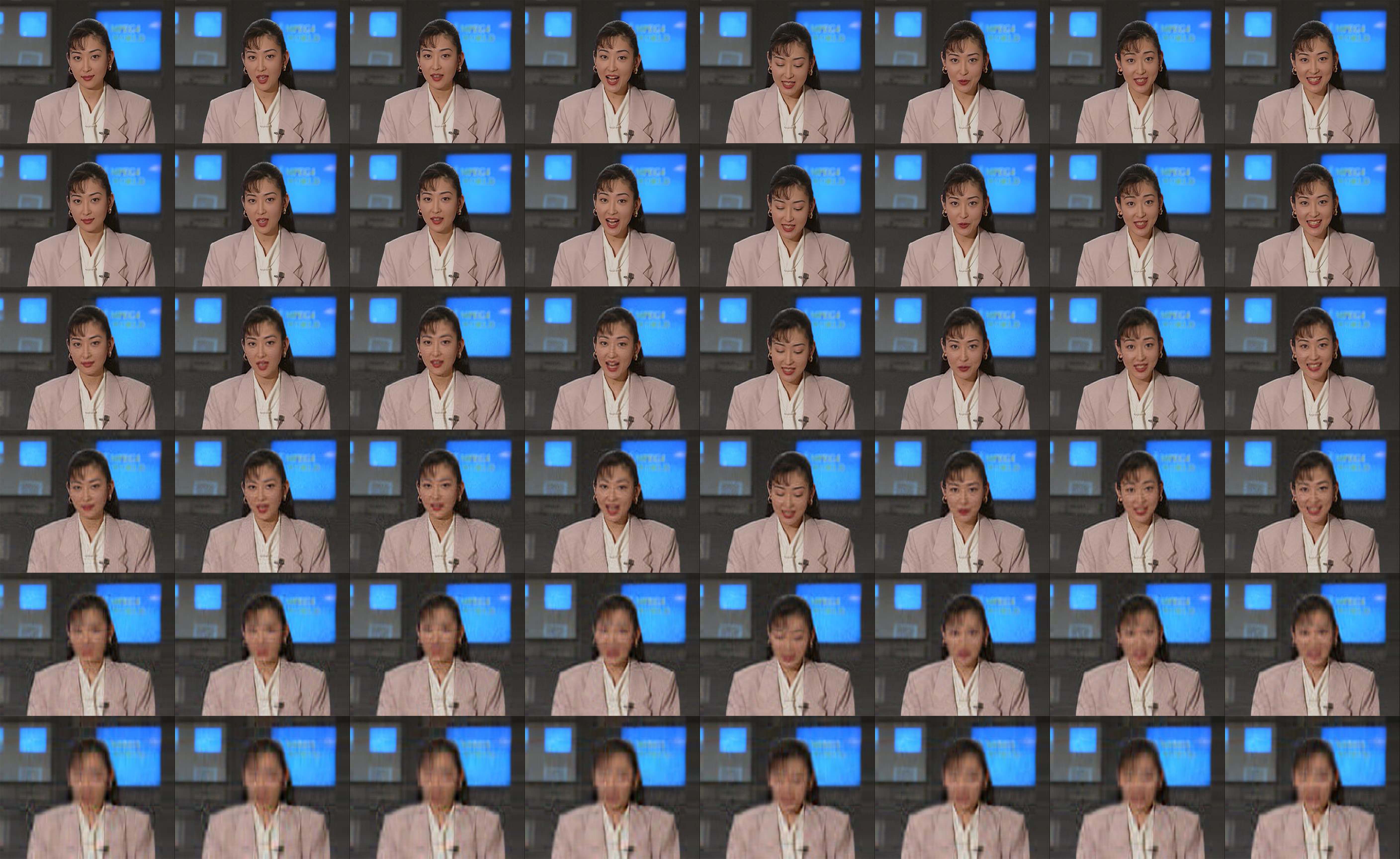
Figure 6.1: Reconstructed results by TS-QHOSVD with different truncated ratios in color video “akiyo”. The first row: the original frames. The second-to-last rows: frames reconstructed by truncated TS-QHOSVD.

Then, we test another color video “carphone”, which was also downloaded from the same website. The video has $382$ frames, each of size $144\times 176$, which results into a pure quaternion tensor in $\mathbb{H}^{382\times 144\times 176}$. The setting is the same as above. The results are presented in Tab. 2. Some reconstructed frames by TS-QHOSVD are illustrated in Fig. 6.2.

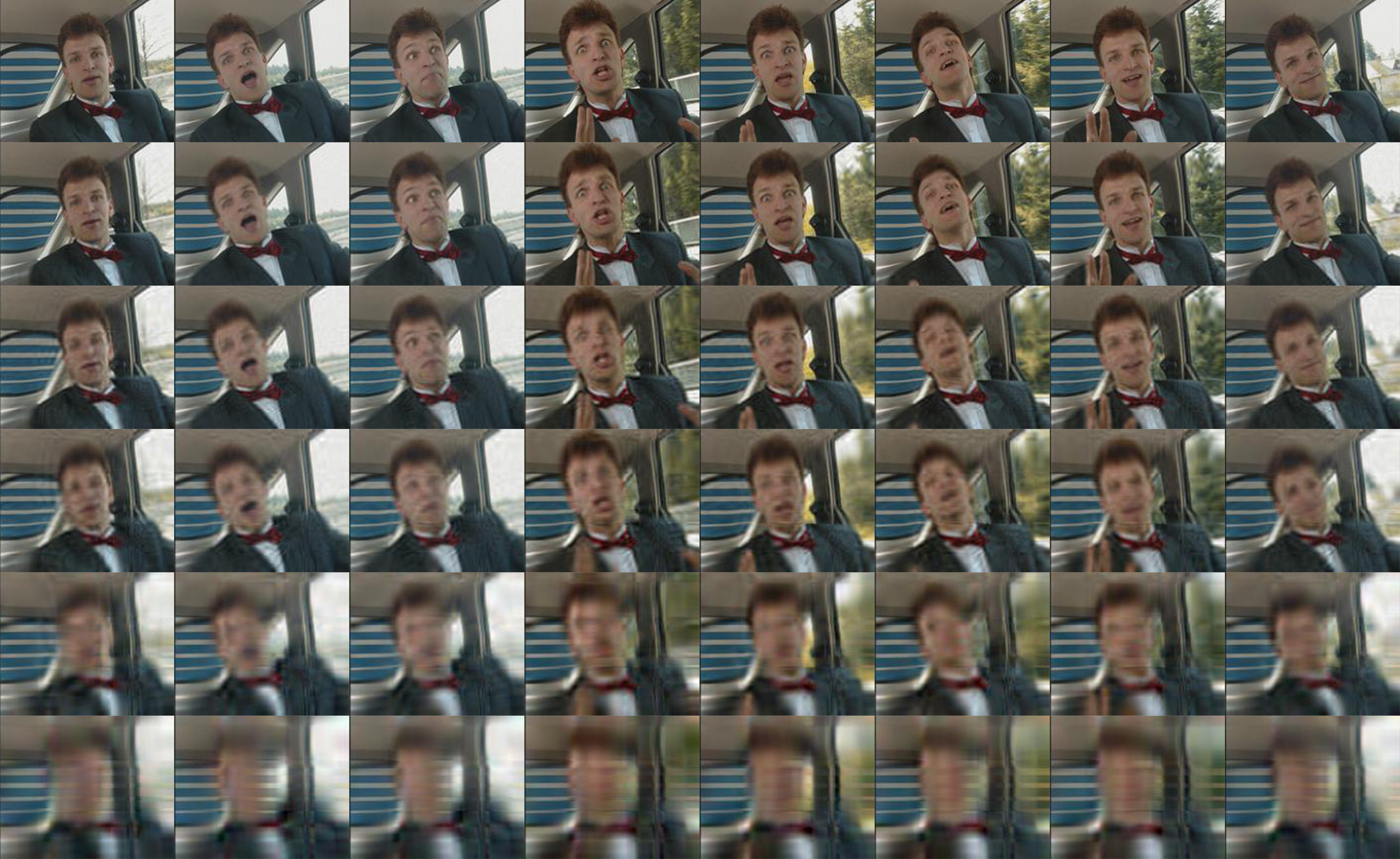
Figure 6.2: Reconstructed results by TS-QHOSVD with different truncated ratios in color video “carphone”. The first row: the original frames. The second-to-last rows: frame reconstructed by truncated TS-QHOSVD

Truncated ratio	TS-QHOSVD		L-QHOSVD		R-QHOSVD		T-HOSVD		ST-HOSVD
	Re.Err	Time	Re.Err	Time	Re.Err	Time	Re.Err	Time	Re.Err	Time
[0.5 0.5 0.5]	$\bm{0.0459}$	3.86	0.0460	3.48	0.0460	3.88	0.0466	5.00	0.0469	$\bm{3.10}$
[0.3 0.3 0.3]	$\bm{0.0747}$	3.12	0.0748	2.65	$\bm{0.0747}$	3.13	0.0757	4.90	0.0765	$\bm{2.56}$
[0.2 0.2 0.2]	$\bm{0.0983}$	2.80	0.0984	2.37	0.0984	2.89	0.0995	4.85	0.1006	$\bm{2.36}$
[0.1 0.1 0.1]	$\bm{0.1440}$	2.55	0.1443	$\bm{1.85}$	0.1445	2.51	0.1461	4.82	0.1476	2.21
[0.05 0.05 0.05]	0.1958	2.45	$\bm{0.1954}$	$\bm{1.66}$	0.1959	2.39	0.1991	4.80	0.2013	2.14

Table 2: Comparisons of truncated TS-, L-, R-QHOSVD, T-HOSVD, and ST-HOSVD on color video “carphone” compression.

From the tables, we observe that concerning the reconstruction error, the three truncated QHOSVDs seem to be comparable, where TS-QHOSVD is slightly better. They are all better than T-HOSVD and ST-HOSVD. This is not surprising, as with the same truncated ratios, the quaternion models consist of more parameters. Concerning the elapsed time, TS-QHOSVD, L-QHOSVD, and R-QHOSVD are comparable; however, if in a suitable parallel computer, we expect that TS-QHOSVD can be speeded up.

At the same time, we compare the absolute error $\|\mathcal{T}-\hat{\mathcal{T}}\|_{F}$ and the tail energy, i.e., the sum of squares of discarded singular values of reconstructed results in the same color videos “akiyo” and “carphone”, which are illustrated in Tab. 3 and Tab. 4, respectively. We see that the tail energy is not far away from the error, showing the meaningfulness of it as an upper bound. In particular, For L- and R-QHOSVD, the tail energy is exactly the error, confirming the results of Theorems 5.2 and 5.3.

Truncated ratio	TS-QHOSVD		L-QHOSVD		R-QHOSVD
	Err	Tail	Err	Tail	Err	Tail
[0.5 0.5 0.5]	60.8320	61.8069	61.2242	61.2242	60.9824	60.9824
[0.3 0.3 0.3]	144.1173	147.2666	145.3070	145.3070	144.1373	144.1373
[0.2 0.2 0.2]	214.9181	220.9655	216.8263	216.8263	215.1406	215.1406
[0.1 0.1 0.1]	326.4334	338.9030	329.4762	329.4762	325.9099	325.9099
[0.05 0.05 0.05]	435.9235	455.4647	438.4096	438.4096	436.2796	436.2796

Table 3: Error and tail energy of reconstructed results by TS-, L- , and R-QHOSVD with different truncated ratios in color video “akiyo” .

Truncated ratio	TS-QHOSVD		L-QHOSVD		R-QHOSVD
	Err	Tail	Err	Tail	Err	Tail
[0.5 0.5 0.5]	107.0193	111.0685	107.2097	107.2097	107.2300	107.2300
[0.3 0.3 0.3]	174.2949	185.3623	174.5917	174.5917	174.3866	174.3866
[0.2 0.2 0.2]	229.2004	245.9943	229.6513	229.6513	229.5991	229.5991
[0.1 0.1 0.1]	335.8326	363.3138	336.5949	336.5949	337.0896	337.0896
[0.05 0.05 0.05]	456.8577	495.0210	455.9724	455.9724	456.9492	456.9492

Table 4: Error and tail energy of reconstructed results by TS-, L- , and R-QHOSVD with different truncated ratios in color video “carphone”.

7 Conclusions

HOSVD [5, 26] is one of the most popular tensor decompositions. Very recently, it was generalized to the quaternion domain [19], which is referred to as L-QHOSVD in this work. L-QHOSVD decomposes the quaternion data tensor as a core tensor left multiplied by factor matrices along each mode, which, due to the non-commutativity of multiplications of quaternions, is not consistent with quaternion matrix SVD when the order of the tensor is $2$. Instead, we proposed a two-sided quaternion HOSVD (TS-QHOSVD) in this work, which is a more natural generalization of the matrix SVD. This is achieved by left and right multiplying the core tensor by factor matrices. TS-QHOSVD admits certain parallel features as the original HOSVD [5]. The ordering and orthogonality properties of the core tensor generated by TS-QHOSVD are investigated. Correspondingly, QHOSVD based on right multiplications (R-QHOSVD) was also introduced. We then studied the truncated TS-, L-, and R-QHOSVD and established their error bounds measured by the tail energy. Due to the non-commutativity, the analysis is nontrivial, which is more complicated than their real or complex counterparts. We also pointed out that the reconstructed tensor may not be a $\sqrt{N}$-suboptimal solution, and may not be of low rank in all modes. Finally, we provided preliminary numerical examples to show the properties of TS-QHOSVD and the efficacy of truncated QHOSVDs.

What makes QHOSVDs different from their real counterparts, what makes TS-, L-, and R-QHOSVD different from each other, and what makes the analysis more difficult? In our understanding, there are three basic reasons: 1) the non-commutativity of quaternion multiplications; 2) the transpose of a unitary quaternion matrix is no longer unitary; 3) a quaternion matrix and its transpose do not share the same SVD and the same rank, and in fact, the last two points are rooted in the first one. How to design a QHOSVD model that maintains more properties from the real counterparts, and how to properly define multilinear rank for quaternion tensors? These still need further research.

Appendix A Proof of Lemma 3.5

We only present the proof of Lemma 3.5, while that for Lemma 3.4 is analogous.

Let $\mathcal{T}\in\mathbb{H}^{I_{1}\times\cdots\times I_{N}}$ and $\mathbf{V}_{m}\in\mathbb{H}^{I_{m}\times J_{m}}(m=1,2,\dots,k)$. Denote

$$\mathbf{G}:=\mathbf{V}_{N}\otimes\cdots\otimes\mathbf{V}_{k}\otimes\mathbf{I}_{k-1}\otimes\cdots\otimes\mathbf{I}_{j+1}\otimes\mathbf{I}_{j-1}\otimes\cdots\otimes\mathbf{I}_{1}.$$

Our goal is to show that every entry $[\mathcal{T}\times^{R}_{N}\mathbf{V}_{N}\cdots\times^{R}_{k}\mathbf{V}_{k}]_{i_{1}\dots i_{k-1}j_{k}\dots j_{N}}$ is the same as the entry $\left((\mathbf{T}^{R}_{[j]})^{T}\mathbf{G}\right)^{T}(r,i_{k})$. From Definition 3.4, we have

$$[\mathcal{T}\times^{R}_{N}\mathbf{V}_{N}\cdots\times^{R}_{k}\mathbf{V}_{k}]_{i_{1}\dots i_{k-1}j_{k}\dots j_{N}}=\sum_{i_{1}=1}^{I_{1}}\cdots\sum_{i_{N}=1}^{I_{N}}t_{i_{1}i_{2}\dots i_{N}}v_{i_{N}j_{N}}\cdots v_{i_{k}j_{k}}.$$

On the other hand, we have

$$\begin{split}\left((\mathbf{T}^{R}_{[j]})^{T}\mathbf{G}\right)^{T}(r,i_{k})=&(\mathbf{T}^{R}_{[j]})^{T}(i_{k},:)\mathbf{G}(:,r)=\sum_{p=1}^{P}\mathbf{T}^{R}_{[j]}(p,i_{k})\mathbf{G}(p,r),\end{split}$$ (A1)

where

$$\begin{split}&P=I_{N}\cdots I_{k+1}I_{k-1}\cdots I_{1};\\ &p=1+\sum_{\begin{subarray}{c}l=1\\ l\neq k\end{subarray}}^{N}\nolimits(i_{l}-1)P_{l}\qquad\text{with}\qquad P_{l}=\prod\nolimits_{\begin{subarray}{c}m=1\\ m\neq k\end{subarray}}^{l-1}I_{m}.\\ &r=1+\sum_{l=1}^{k-1}(i_{l}-1)R_{l}+\sum_{l=k+1}^{N}(j_{l}-1)R_{l}\qquad\text{with}\\ &R_{l}=\begin{cases}\prod\nolimits_{\begin{subarray}{c}d=1\end{subarray}}^{l-1}I_{d},&l<k\\ \prod\nolimits_{\begin{subarray}{c}d=1\end{subarray}}^{k-1}I_{d},&l=k+1\\ (\prod\nolimits_{\begin{subarray}{c}d=1\end{subarray}}^{k-1}I_{d})(\prod\nolimits_{\begin{subarray}{c}d=k+1\end{subarray}}^{l-1}J_{d}),&l>k+1.\end{cases}\\ \end{split}$$

From the definition of Kronecker product we have

$$\mathbf{G}(p,r)=\mathbf{V}_{N}(i_{N},j_{N})\cdots\mathbf{V}_{k}(i_{k},j_{k})\mathbf{I}(i_{k-1},i_{k-1})\cdots\mathbf{I}(i_{1},i_{1})=\mathbf{V}_{N}(i_{N},j_{N})\cdots\mathbf{V}_{k}(i_{k},j_{k}).$$

Note that $\mathbf{T}^{R}_{[j]}(p,i_{k})=t_{i_{1}i_{2}\dots i_{N}}$ and $\mathbf{V}(i_{k},j_{k})=v_{i_{k}j_{k}}$. Thus, we can rewrite (A1) as

$$\left((\mathbf{T}^{R}_{[j]})^{T}\mathbf{G}\right)^{T}(r,i_{k})=\sum_{i_{1}=1}^{I_{1}}\cdots\sum_{i_{N}=1}^{I_{N}}t_{i_{1}i_{2}\dots i_{N}}v_{i_{N}j_{N}}\cdots v_{i_{k}j_{k}}.$$

And when $j=k$, $\mathcal{Y}\times^{R}_{k}\mathbf{V}_{k}^{H}=\mathcal{T}\times^{R}_{N}\mathbf{V}_{N}\cdots\times^{R}_{k-1}\mathbf{V}_{k-1}$. Therefore we have

$$\mathbf{Y}^{R}_{[k]}\mathbf{V}_{k}^{H}=\left((\mathbf{T}^{R}_{[j]})^{T}(\mathbf{V}_{N}\otimes\cdots\otimes\mathbf{V}_{j+1}\otimes\mathbf{I}_{j-1}\otimes\cdots\otimes\mathbf{I}_{1})\right)^{T},$$

namely,

$$\mathbf{Y}^{R}_{[k]}=\left((\mathbf{T}^{R}_{[j]})^{T}(\mathbf{V}_{N}\otimes\cdots\otimes\mathbf{V}_{j+1}\otimes\mathbf{I}_{j-1}\otimes\cdots\otimes\mathbf{I}_{1})\right)^{T}\mathbf{V}_{k}.$$

From the above, consider the special case of $\mathbf{V}_{q}=\mathbf{I}_{q}(q\neq i_{k})$. Then its right mode-$j$ unfolding is

$$\mathbf{Y}^{R}_{[j]}=\left((\mathbf{T}^{R}_{[j]})^{T}\mathbf{H}\right)^{T},$$

where

$$\mathbf{H}=\mathbf{I}_{N}\otimes\cdots\otimes\mathbf{I}_{i_{k}+1}\otimes\mathbf{V}_{i_{k}}\otimes\mathbf{I}_{i_{k}-1}\otimes\cdots\otimes\mathbf{I}_{i_{i-1}+1}\otimes\mathbf{V}_{i_{k-1}}\otimes\mathbf{I}_{i_{k-1}-1}\otimes\cdots\\ \otimes\mathbf{I}_{i_{1}+1}\otimes\mathbf{V}_{i_{1}}\otimes\mathbf{I}_{i_{1}-1}\otimes\cdots\otimes\mathbf{I}_{j+1}\otimes\mathbf{I}_{j-1}\otimes\cdots\otimes\mathbf{I}_{1}.$$

Appendix B Tensors in Example 1

The original tensor $\mathcal{T}$ is

$$\mathcal{T}(:,:,1,1)=\begin{bmatrix}\begin{smallmatrix}0.5377+0.2916i-1.1201j-0.0290k&0.8622-0.8045i+0.3075j-0.0845k&-0.4336-0.2437i-0.1765j+0.414k\\ 1.8339+0.1978i+2.5260j+0.1825k&0.3188+0.6966i-1.2571j+1.6039k&0.3426+0.2157+0.7914j-0.7342k\\ -2.2577+1.5877i+1.6555j-1.5651k&-1.3077+0.8351i-0.8655j+0.0983k&3.5784-1.1658i-1.3320j-0.0308k\end{smallmatrix}\end{bmatrix};$$

$$\mathcal{T}(:,:,1,2)=\begin{bmatrix}\begin{smallmatrix}-0.3034+1.7119i-0.0679j+0.3271k&0.8884-0.8396i-0.3031j-0.6509k&-0.8095+0.9610i+0.8261j-1.3218k\\ 0.2939-0.1941i-0.1952j+1.0826k&-1.1471+1.3546i+0.0230j+0.2571k&-2.9443+0.1240i+1.5270j+0.9248k\\ -0.7873-2.1384i-0.2176j+1.0061k&-1.0689-1.0722i+0.0513j-0.9444k&1.4384+1.4367i+0.4669j+4.9849e-05k\end{smallmatrix}\end{bmatrix};$$

$$\mathcal{T}(:,:,1,3)=\begin{bmatrix}\begin{smallmatrix}-0.0068+0.0335i-0.1922j+0.5812k&0.3714+0.3502i-0.2490j+0.0799k&-1.0891-0.2620i+1.2347j+0.6770k\\ 1.5326-1.3337i-0.2741j-2.1924k&-0.2256-0.2991i-1.0642j-0.9485k&0.0326-1.7502i-0.2296j+0.8577k\\ -0.7697+1.1275i+1.5301j-2.3193k&1.1174+0.0229i+1.6035j+0.4115k&0.5525-0.2857i-1.5062j-0.6912k\end{smallmatrix}\end{bmatrix};$$

$$\mathcal{T}(:,:,2,1)=\begin{bmatrix}\begin{smallmatrix}2.7694-1.1480i-2.3299j+0.2323k&0.7254+2.5855i+0.3914j-0.2365k&-0.2050-0.0825i+0.1837j+2.2294k\\ -1.3499+0.1049i-1.4491j+0.4264k&-0.0631-0.6669i+0.4517j+2.0237k&-0.1241-1.9330i-0.04762j+0.3376k\\ 3.0349+0.7223i+0.3335j-0.3728k&0.7147+0.1837i-0.1303j-2.2584k&1.4897-0.4390i+0.8620j+1.0001k\end{smallmatrix}\end{bmatrix};$$

$$\mathcal{T}(:,:,2,2)=\begin{bmatrix}\begin{smallmatrix}0.3252-1.9609i-0.2097j-0.0549k&-1.7115+2.9080i-1.0298j+0.3502k&0.3192-1.0582i+0.1352j+0.2398k\\ -0.7549-0.1977i+0.6252j+0.9111k&-0.1022+0.8252i+0.9492j+1.2503k&0.3129-0.4686i+0.5152j-0.6904k\\ 1.3703-1.2078i+0.1832j+0.5946k&-0.2414+1.3790i+0.3071j+0.9298k&-0.8649-0.2725i+0.2614j-0.6516k\end{smallmatrix}\end{bmatrix};$$

$$\mathcal{T}(:,:,2,3)=\begin{bmatrix}\begin{smallmatrix}1.1006-0.8314i-0.4446j+0.4494k&-1.4916-0.5336i-0.2612j+0.5362k&2.3505+0.5201i-1.2507j-0.1472k\\ 1.5442-0.9792i-0.1559j+0.1006k&-0.7423-2.0026i+0.4434j+0.8979k&-0.6156-0.0200i-0.9480j+1.0078k\\ 0.0859-1.1564i+0.2761j+0.8261k&-1.0616+0.9642i+0.3919j-0.1319k&0.7481-0.0348i-0.7411j-2.1238k\end{smallmatrix}\end{bmatrix};$$

$$\mathcal{T}(:,:,3,1)=\begin{bmatrix}\begin{smallmatrix}1.4090-1.7947i-1.3617j-1.6642k&-1.2075+0.1001i-0.3349j-0.4227k&0.4889-0.6003i-1.1176j-1.2128k\\ 1.4172+0.8404i+0.4550j-0.5900k&0.7172-0.5445i+0.5528j-1.6702k&1.0347+0.4900i+1.2607j+0.0662k\\ 0.6715-0.8880i-0.8487j-0.2781k&1.6302+0.3035i+1.0391j+0.4716k&0.7269+0.7394i+0.6601j+0.6524k\end{smallmatrix}\end{bmatrix};$$

$$\mathcal{T}(:,:,3,2)=\begin{bmatrix}\begin{smallmatrix}-0.0301+1.0984i-0.9415j+1.1921k&1.0933-2.0518i-0.5320j-1.9488k&0.0774-1.5771i-0.4838j+0.0012k\\ -0.1649-0.2779i-0.1623j-1.6118k&1.1093-0.3538i+1.6821j+1.0205k&-1.2141+0.5080i-0.7120j-0.0708k\\ 0.6277+0.7015i-0.1461j-0.0245k&-0.8637-0.8236i-0.8757j+0.8617&-1.1135+0.2820i-1.1742j-2.4863k\end{smallmatrix}\end{bmatrix};$$

$$\mathcal{T}(:,:,3,3)=\begin{bmatrix}\begin{smallmatrix}-0.1924-0.7982i-0.5078j-0.5046k&-1.4023-0.7145i-3.0292j+0.6487k&-0.1774-0.5890i-1.0667j+0.6487k\\ 0.8886+1.0187i-0.3206j-1.2706k&-1.4224+1.3514i-0.4570j+0.8257k&-0.1961-0.2938i+0.9337j+0.1370k\\ -0.7648-0.1332i+0.0125j-0.3826k&0.4882-0.2248i+1.2424j-1.0149k&1.4193-0.8479i+0.3503j-0.2919k\end{smallmatrix}\end{bmatrix}.$$

Applying TS-QHOSVD to $\mathcal{T}$, the factor matrices are

$$\mathbf{U}_{1}=\begin{bmatrix}\begin{smallmatrix}-0.5993&0.1523j-0.5458k&0.5654\\ 0.1969-0.1997i-0.0229j-0.0205k&0.5241-0.1718i-0.2519j-0.4259k&-0.1346+0.1462i-0.0489-0.5740k\\ -0.1692+0.5742i+0.2845j+0.3521k&0.2197-0.2700i+0.0789j+0.0491k&-0.1532+0.5174i+0.1001j+0.0884k\end{smallmatrix}\end{bmatrix};$$

$$\mathbf{U}_{2}=\begin{bmatrix}\begin{smallmatrix}0.5714j-0.2928k&-0.0745j-0.6417k&0.2062j+0.3577k\\ -0.4038+0.1277i-0.0657j+0.2431k&0.2835+0.5351i-0.3617j+0.0491k&-0.0918+0.3075i-0.1065j+0.3781k\\ -0.0281-0.3679i-0.1627j-0.4271k&0.0330+0.0608i+0.2135j+0.1798k&0.5833+0.0925i-0.2325j+0.4115k\end{smallmatrix}\end{bmatrix};$$

$$\mathbf{V}_{3}=\begin{bmatrix}\begin{smallmatrix}-0.6752&0.5114-0.0471i+0.2838j-0.3166k&-0.0513-0.2257i+0.0305j+0.2128k\\ 0.5994j-0.0105k&-0.2351-0.0446i+0.5412j-0.0057k&-0.4799+0.2295i+0.0659j-0.0559k\\ -0.3987j-0.1605k&-0.0505+0.4426i-0.0194j-0.0820k&-0.5720-0.2582i+0.3223j-0.3347k\end{smallmatrix}\end{bmatrix};$$

$$\mathbf{V}_{4}=\begin{bmatrix}\begin{smallmatrix}-0.2329j+0.8308k&-0.1488-0.0865i+0.3140j+0.1322k&-0.0845+0.0620i-0.1707j+0.2642k\\ -0.2667j-0.0031k&0.2033+0.1125i-0.2918j-0.6755k&0.1561+0.1842i-0.2166j+0.4777k\\ 0.4295j-0.0048k&0.2107-0.2687i-0.2686j+0.2648k&-0.0676-0.0158i-0.7332j+0.1194k\end{smallmatrix}\end{bmatrix}.$$

The core tensor $\mathcal{S}$ is

$$\mathcal{S}(:,:,1,1)=\begin{bmatrix}\begin{smallmatrix}1.7081-3.5317i+2.3532j+0.0446k&-1.1102-3.1816i-1.5091j-0.6175k&1.4489-1.2615i+0.7234j+2.1912k\\ -2.6019+0.3027i-0.6953j-0.4676k&-1.4555-0.2297i-0.2625j-0.0222k&1.1954+0.4502i-0.5930j+1.9834k\\ 0.2443-0.9830i+1.1293j+1.4397k&-1.7384-0.9887i+0.9757j-1.6732k&0.2000+1.4965i+0.1288j+0.914k\end{smallmatrix}\end{bmatrix};$$

$$\mathcal{S}(:,:,1,2)=\begin{bmatrix}\begin{smallmatrix}-2.5860-0.2759i-0.8616j-0.3308k&0.8777+04209i+0.2807j+0.0630k&-1.0578+08603i-0.5296j+0.3823k\\ -0.6324+0.1781i-1.2702j-0.6573k&-2.4700+0.7213i-0.9573j+1.8586k&0.1192-1.5597i+0.6392j+0.1053k\\ -0.8903-0.2137i+1.1123j-0.5548k&0.9992-2.2155i+0.7875j+0.3975k&-0.8117-1.1676i+0.3125j+0.6657k\end{smallmatrix}\end{bmatrix};$$

$$\mathcal{S}(:,:,1,3)=\begin{bmatrix}\begin{smallmatrix}-0.6866-0.0981i-1.2687j-1.6193k&-0.3959-1.9493i-0.2269j-1.5476k&-1.2495+0.1875i-1.7158j+0.1577k\\ -1.1016-0.9181i+0.9518j-0.0598k&-0.2174+1.8719i-1.6428j-0.3110k&0.7502-0.3142i+1.8509j+0.8731k\\ 0.9637+0.0746i-0.0371j+0.4866k&0.9154+1.5161i-0.9982j-0.2489k&0.2718-0.0757i+1.2910j-0.7688k\end{smallmatrix}\end{bmatrix};$$

$$\mathcal{S}(:,:,2,1)=\begin{bmatrix}\begin{smallmatrix}1.7941+3.6683i+0.1602j-1.3770k&0.6149-1.6978i+0.7166-0.2762k&-0.9569-1.1475i-0.7704j-0.2525k\\ -1.5855+2.9859i+0.6551j-0.2816k&-0.2745+0.1111i+0.9195j-1.3344k&0.8033-0.0622i-0.5005j-0.5929k\\ 0.9913-0.7520i+0.1230j-0.8184k&-1.6733-1.0918i+0.4341j+0.1745k&1.6396-1.8814i+0.2802j+1.1155k\end{smallmatrix}\end{bmatrix};$$

$$\mathcal{S}(:,:,2,2)=\begin{bmatrix}\begin{smallmatrix}0.3924+0.2386i+0.3920j+0.7215k&-0.8570-0.9868i-0.5928j+0.4893k&-0.3009-1.2083i+1.1496j-0.3629k\\ -3.1245+0.3278i-0.6232j-1.8169k&0.4772+0.5001i+1.2240j-0.2122k&0.0582+0.4981i+0.7100j+0.8256k\\ 0.3591+1.1232i-1.2438j-1.2502k&-1.6865-0.6055i-0.5717j+0.5051k&-0.5729-0.4912i-0.5238j+0.5424k\end{smallmatrix}\end{bmatrix};$$

$$\mathcal{S}(:,:,2,3)=\begin{bmatrix}\begin{smallmatrix}-1.9728-0.7386i-1.6027j-0.8238k&0.5102+1.0492i+0.2651j+0.1651k&-1.0522-0.4281i-0.6517j-0.1413k\\ 0.5983+0.9513i-0.9909j+0.6030k&-0.1637+0.4230i+0.8125j-0.9651k&-1.3644-0.1076i+0.6987j-0.4524k\\ 0.2266+0.2795i-0.0132j+0.8986k&-0.8485+2.0576i-0.0949j+1.1471k&0.6144+0.8572i+0.0591j+0.5176k\end{smallmatrix}\end{bmatrix};$$

$$\mathcal{S}(:,:,3,1)=\begin{bmatrix}\begin{smallmatrix}-0.0909-1.2885i+0.5919j-0.2144k&0.9613+0.3602i+2.7605j-0.8544k&-0.8568+0.4285i-0.5396j+0.4078k\\ -1.7391-1.0238i-1.3144j-0.8129k&-0.9227+0.7464i+0.5385j-0.0288k&1.1027+1.7074i-0.2325j-0.2929k\\ -0.7938+1.3105i-0.8440j+0.0815k&-0.5404+0.0954i-1.1640j+0.7876k&-1.2313-0.4745i+0.12230j+0.6916k\end{smallmatrix}\end{bmatrix};$$

$$\mathcal{S}(:,:,3,2)=\begin{bmatrix}\begin{smallmatrix}-2.2683-2.0462i+0.1989j+2.1435k&-0.1576-1.3004i-1.2320j-2.3784k&0.5365+0.3068i+0.0604j-0.6186k\\ 0.7398-0.9730i+1.4379j=0.5570K&-0.2262+0.4788i-0.1488j+0.3944k&-1.4164-1.5279i+0.5121j+0.0930k\\ 0.3966+0.7416i-0.3880j-0.8873k&-1.0336+0.5844i+0.6076j-0.8540k&0.4865+0.0907i-0.4744j-0.1661k\end{smallmatrix}\end{bmatrix};$$

$$\mathcal{S}(:,:,3,3)=\begin{bmatrix}\begin{smallmatrix}0.4157-0.3102i+0.9778j+0.6745k&0.8750+0.4594i-0.5408j+0.1177k&0.5977+0.6328i-0.0953j-1.3262k\\ 1.3408-0.6202i-0.5694j+0.2075k&0.2980+1.3948i+1.8697j+0.4938k&0.7614+0.7278i+0.9163j-0.1965k\\ 0.0114+0.1545i+0.1161j+0.9844k&-0.0074+0.6996i+0.3834j+1.0026k&-0.1529+0.6077i+0.2344j+0.1759k\end{smallmatrix}\end{bmatrix}.$$

References

- [1] J. Chen and M. K. Ng, Color image inpainting via robust pure quaternion matrix completion: Error bound and weighted loss, SIAM J. Imag. Sci., 15 (2022), pp. 1469–1498.
- [2] A. Cichocki, D. Mandic, L. De Lathauwer, G. Zhou, Q. Zhao, C. Caiafa, and H. A. Phan, Tensor decompositions for signal processing applications: From two-way to multiway component analysis, IEEE Signal Process. Mag., 32 (2015), pp. 145–163.
- [3] P. Comon, Tensors: a brief introduction, IEEE Signal Process. Mag., 31 (2014), pp. 44–53.
- [4] L. De Lathauwer, Decompositions of a higher-order tensor in block terms—part I: Lemmas for partitioned matrices, SIAM J. Matrix Anal. Appl., 30 (2008), pp. 1022–1032.
- [5] L. De Lathauwer, B. De Moor, and J. Vandewalle, A multilinear singular value decomposition, SIAM J. Matrix Anal. Appl., 21 (2000), pp. 1253–1278.
- [6] Z.-H. He, X.-X. Wang, and Y.-F. Zhao, Eigenvalues of quaternion tensors with applications to color video processing, J. Sci. Comput., 94 (2023), p. 1.
- [7] O. Imhogiemhe, J. Flamant, X. Luciani, Y. Zniyed, and S. Miron, Low-rank tensor decompositions for quaternion multiway arrays, in ICASSP 2023-2023 IEEE International Conference on Acoustics, Speech and Signal Processing (ICASSP), IEEE, 2023, pp. 1–5.
- [8] Z. Jia, Q. Jin, M. K. Ng, and X.-L. Zhao, Non-local robust quaternion matrix completion for large-scale color image and video inpainting, IEEE Trans. Image Process., 31 (2022), pp. 3868–3883.
- [9] Z. Jia and M. K. Ng, Structure preserving quaternion generalized minimal residual method, SIAM J. Matrix Anal. Appl., 42 (2021), pp. 616–634.
- [10] Z. Jia, M. K. Ng, and G.-J. Song, Lanczos method for large-scale quaternion singular value decomposition, Numer. Algorithms, 82 (2019), pp. 699–717.
- [11] , Robust quaternion matrix completion with applications to image inpainting, Numer. Linear Algebra Appl., 26 (2019), p. e2245.
- [12] Z. Jia, M. Wei, M.-X. Zhao, and Y. Chen, A new real structure-preserving quaternion qr algorithm, J. Comput. Applied Math., 343 (2018), pp. 26–48.
- [13] M. E. Kilmer and C. D. Martin, Factorization strategies for third-order tensors, Linear Algebra Appl., 435 (2011), pp. 641–658.
- [14] T. G. Kolda and B. W. Bader, Tensor decompositions and applications, SIAM Rev., 51 (2009), pp. 455–500.
- [15] J. Miao and K. I. Kou, Quaternion-based bilinear factor matrix norm minimization for color image inpainting, IEEE Trans. Signal Process., 68 (2020), pp. 5617–5631.
- [16] J. Miao and K. I. Kou, Quaternion tensor singular value decomposition using a flexible transform-based approach, Signal Process., 206 (2023), p. 108910.
- [17] J. Miao, K. I. Kou, D. Cheng, and W. Liu, Quaternion higher-order singular value decomposition and its applications in color image processing, Inf. Fusion, 92 (2023), pp. 139–153.
- [18] J. Miao, K. I. Kou, and W. Liu, Low-rank quaternion tensor completion for recovering color videos and images, Pattern Recognit., 107 (2020), p. 107505.
- [19] J. Miao, K. I. Kou, L. Yang, and D. Cheng, Quaternion tensor train rank minimization with sparse regularization in a transformed domain for quaternion tensor completion, 2022.
- [20] S. Miron, J. Flamant, N. Le Bihan, P. Chainais, and D. Brie, Quaternions in signal and image processing: A comprehensive and objective overview, IEEE Signal Process. Mag., 40 (2023), pp. 26–40.
- [21] I. V. Oseledets, Tensor-train decomposition, SIAM J. Sci. Comput., 33 (2011), pp. 2295–2317.
- [22] L. Qi, Z. Luo, Q.-W. Wang, and X. Zhang, Quaternion matrix optimization: Motivation and analysis, J. Optim. Theory Appl., 193 (2022), pp. 621–648.
- [23] Z. Qin, Z. Ming, and L. Zhang, Singular value decomposition of third order quaternion tensors, Applied Math. Lett., 123 (2022), p. 107597.
- [24] L. Rodman, Topics in Quaternion Linear Algebra, Princeton University Press, 2014.
- [25] N. D. Sidiropoulos, L. De Lathauwer, X. Fu, K. Huang, E. E. Papalexakis, and F. C., Tensor decomposition for signal processing and machine learning, IEEE Trans. Signal Process., 65 (2017), pp. 3551–3582.
- [26] N. Vannieuwenhoven, R. Vandebril, and K. Meerbergen, A new truncation strategy for the higher-order singular value decomposition, SIAM J. Sci. Comput., 34 (2012), pp. A1027–A1052.
- [27] M. Wei, Y. Li, F. Zhang, and J. Zhao, Quaternion matrix computations, Nova Science Publishers, Incorporated, 2018.
- [28] D. Xu and D. P. Mandic, The theory of quaternion matrix derivatives, IEEE Trans. Signal Process., 63 (2015), pp. 1543–1556.
- [29] D. Xu, Y. Xia, and D. P. Mandic, Optimization in quaternion dynamic systems: Gradient, hessian, and learning algorithms, IEEE Trans. Neural Netw. Learn. Syst., 27 (2015), pp. 249–261.
- [30] F. Zhang, Quaternions and matrices of quaternions, Linear Algebra Appl., 251 (1997), pp. 21–57.
- [31] Q. Zhao, G. Zhou, S. Xie, L. Zhang, and A. Cichocki, Tensor ring decomposition, arXiv preprint arXiv:1606.05535, (2016).
- [32] M.-M. Zheng and G. Ni, Approximation strategy based on the t-product for third-order quaternion tensors with application to color video compression, Applied Math. Lett., 140 (2023), p. 108587.
- [33] C. Zou, K. I. Kou, and Y. Wang, Quaternion collaborative and sparse representation with application to color face recognition, IEEE Trans. Image Process., 25 (2016), pp. 3287–3302.
- [34] C. Zou, K. I. Kou, Y. Wang, and Y. Y. Tang, Quaternion block sparse representation for signal recovery and classification, Signal Process., 179 (2021), p. 107849.